Rural E-Commerce and Multi-Scale Spatial Reorganization: Within-County Concentration and Intercounty Differentiation in China

Abstract

Rural e-commerce has expanded market access and economic opportunities in rural areas, yet its implications for the spatial organization of economic activity remain less understood. This study examines whether China’s Comprehensive Demonstration Program for E-Commerce in Rural Areas reshapes economic activity within counties and across counties within the same prefecture-level city. Using county-level panel data from 2011 to 2024, we combine nighttime-light and impervious-surface data to construct measures of within-county spatial concentration (WSC) and city-relative gap (CRG), and exploit the staggered policy rollout in a difference-in-differences framework. The results show that policy implementation significantly increases within-county concentration and is associated with greater differentiation from contemporaneous same-city peers, with the baseline estimates equivalent to approximately 1.5% and 4.4% of their respective sample means. Support is stronger for WSC, although its magnitude is sensitive to province-by-year adjustment; the CRG evidence is weaker and estimator-sensitive. Further analyses show that pre-existing core locations strengthen their relative position after policy implementation, while county-relative differentiation responds more strongly at lower levels of initial market density. Overall, the results show that market integration and spatial convergence are distinct dimensions of rural digital development, implying that rural e-commerce policies should be assessed not only by aggregate gains but also by the spatial distribution of economic activity and the differing needs of counties with different market foundations.

1. Introduction

Digital technologies are reshaping the spatial organization of economic activity by reducing information, matching, and market-entry costs and connecting previously isolated producers and consumers to broader markets [1]. These changes are particularly relevant for rural areas, where geographic distance, fragmented distribution networks, and limited local demand have historically constrained economic participation [2]. A growing literature documents the developmental benefits of rural e-commerce, including improvements in local economic activity, household income, and market participation [3,4]. Yet aggregate development outcomes provide limited insight into how the resulting economic opportunities are distributed across space. In particular, it remains unclear whether digital market expansion reshapes economic activity within counties and simultaneously alters the relative economic positions of counties within broader regional systems.

Existing research has documented a wide range of economic effects of rural e-commerce, including county-level growth, household income, business development, employment, industrial restructuring, and urban–rural inequality [3,5]. As attention has shifted from aggregate outcomes toward distributional and spatial effects, a growing literature has examined regional disparities and spatial inequality associated with e-commerce. However, existing studies have largely focused on urban–rural gaps, broad cross-regional differences, or prefecture-level spatial patterns [6,7]. Yu et al. examine county economic development and inequality using the rural e-commerce demonstration program and nighttime-light data, while Lu and Wang construct a nighttime-light-based inequality measure at the prefecture level and analyze within-city inequality and intercity spatial spillovers [7,8]. These studies highlight the spatial implications of rural e-commerce development. Further examination of the distribution of activity within developed space can help establish how locations identified as cores before policy adoption subsequently perform. At the intercounty level, a county-specific measure of the absolute gap from the average of same-city peers can complement prefecture-wide measures of inequality. Within-county concentration and county-relative gaps capture different dimensions of spatial adjustment. Activity may become more concentrated inside a county while its average intensity moves closer to, or further from, that of its same-city peers. Examining both outcomes therefore helps assess whether the policy is accompanied by local concentration, wider county-relative gaps, or both.

To address these questions, this study exploits the staggered rollout of China’s Comprehensive Demonstration Program for E-Commerce in Rural Areas and constructs county-level panel data for 2011–2024 by combining nighttime-light data with developed-space information from the China Land Cover Dataset (CLCD). A staggered difference-in-differences (DID) framework is employed to identify the spatial effects of rural e-commerce. This study contributes in three main respects. First, this study shifts the analysis from aggregate development and inequality outcomes to the spatial reorganization of economic activity. Rather than asking only whether counties become more or less unequal, we examine how policy-induced market expansion is distributed across locations within counties and how counties adjust relative to their contemporaneous peers within the same prefecture-level system. This nested perspective distinguishes internal spatial restructuring from changes in counties’ relative regional positions. Second, it incorporates developed-space information into the measurement of within-county concentration and tests whether the estimates persist within a fixed pre-policy footprint. This makes the spatial domain of measurement explicit and addresses sensitivity to changes in the observed developed area. Third, it tracks core locations defined before policy implementation and examines variation in the county-relative effect by initial market density. These analyses provide evidence on how spatial responses relate to conditions established before the program.

2. Theoretical Analysis and Research Hypotheses

2.1. The Comprehensive Demonstration Program for E-Commerce in Rural Areas

To address weaknesses in rural distribution networks, high logistics costs, and limited market information, the Ministry of Finance and the Ministry of Commerce launched the Comprehensive Demonstration Program for E-Commerce in Rural Areas in successive batches beginning in 2014, with counties serving as the basic units of implementation. Central fiscal support is primarily directed toward county–township–village logistics systems, public e-commerce services, agricultural supply chains, and related training. The program is therefore not merely a digital-access initiative, but an integrated market-development policy combining digital platforms with logistics, warehousing, and public-service infrastructure [9].

This institutional design has an explicit spatial dimension. The location of county-level e-commerce service centers, warehousing facilities, and logistics nodes depends on population concentration, transport accessibility, and existing commercial foundations, and may therefore reshape the internal spatial organization of economic activity [10,11]. At the same time, the expansion of market access may generate uneven responses across counties because of differences in local market conditions and absorptive capacity [9]. The program thus provides an institutional basis for examining both within-county spatial concentration and changes in counties’ relative positions within prefecture-level city systems.

2.2. Rural E-Commerce and Multi-Scale Spatial Reorganization

Rural e-commerce reduces information, matching, and market-entry costs and expands the effective market accessible to rural economic agents [2,12]. However, expanded market access does not imply spatially uniform adjustment. Converting new market opportunities into local economic activity still depends on offline complementary conditions, such as logistics, commercial services, labor, and infrastructure, many of which exhibit fixed costs and economies of scale [9,13]. The spatial consequences of rural e-commerce therefore arise from the interaction between expanded market access and pre-existing local complementarities.

This interaction can produce spatial reorganization at multiple geographic scales. Within counties, existing spatial differences may shape which locations capture a larger share of additional economic activity. Across counties, differences in local capabilities may generate uneven responses to the same policy-induced market expansion. Rural e-commerce may therefore reshape both the internal distribution of economic activity within counties and the relative economic positions of counties within the same prefecture-level city.

2.2.1. Pre-Existing Core Reinforcement and Within-County Spatial Concentration

Economic activity within rural counties is typically unevenly distributed before the introduction of e-commerce policy. County seats, central towns, transport nodes, and other established economic centers generally possess denser commercial activity, better accessibility, and more developed public and business services [10,14]. These advantages are cumulative: the concentration of firms, consumers, infrastructure, and services reduces coordination costs and improves access to specialized inputs, allowing established locations to maintain stronger positions within the local spatial economy [15,16].

Against this uneven spatial structure, established core locations are better positioned to accommodate additional e-commerce-related activity [17]. They can operate at lower average costs and provide denser matching opportunities among firms, logistics providers, workers, and service organizations [15]. Expanded digital market access may therefore increase the value of existing local agglomeration rather than neutralize it [9]. As core locations capture a larger share of additional activity, their relative advantage over non-core developed areas may strengthen, increasing the spatial concentration of economic activity within the county [18].

Importantly, greater within-county concentration does not require economic activity outside the core to decline in absolute terms. Concentration can increase whenever pre-existing core locations expand more rapidly than non-core areas. Rural e-commerce may therefore broaden the external market available to a county while simultaneously reinforcing its internal spatial hierarchy.

H1. 

The rural e-commerce demonstration program increases within-county spatial concentration.

2.2.2. Uneven County Responses and Intercounty Differentiation

At the intercounty scale, counties within the same prefecture-level city differ in their capacity to translate improved market access into local economic activity [19]. Differences in industrial foundations, logistics capacity, commercial services, accessibility, and market networks can therefore generate uneven responses to the same policy shock [9,20].

Importantly, heterogeneous responses do not necessarily increase intercounty differentiation. Counties may respond differently in ways that narrow, preserve, or widen their relative gaps. Intercounty differentiation increases when heterogeneous responses reinforce existing relative differences, moving counties further from their contemporaneous same-city peer benchmarks. This pattern may arise when counties already above their peer benchmarks experience stronger gains, while those below their benchmarks adjust more slowly [21]. Rural e-commerce may therefore amplify differences in counties’ relative economic positions within the same prefecture-level city system.

Beyond this average effect, initial market density may condition the magnitude of intercounty differentiation [9]. In denser markets, established demand, firms, and service networks provide multiple channels for adjustment, making the marginal policy effect more incremental [17]. In thinner markets, responses depend more strongly on a limited set of county-specific industrial, logistical, and market complementarities [22]. Policy responses may therefore be more selective, making counties’ relative positions more sensitive to rural e-commerce expansion.

H2. 

The rural e-commerce demonstration program increases intercounty differentiation within prefecture-level city systems.

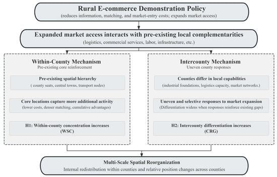
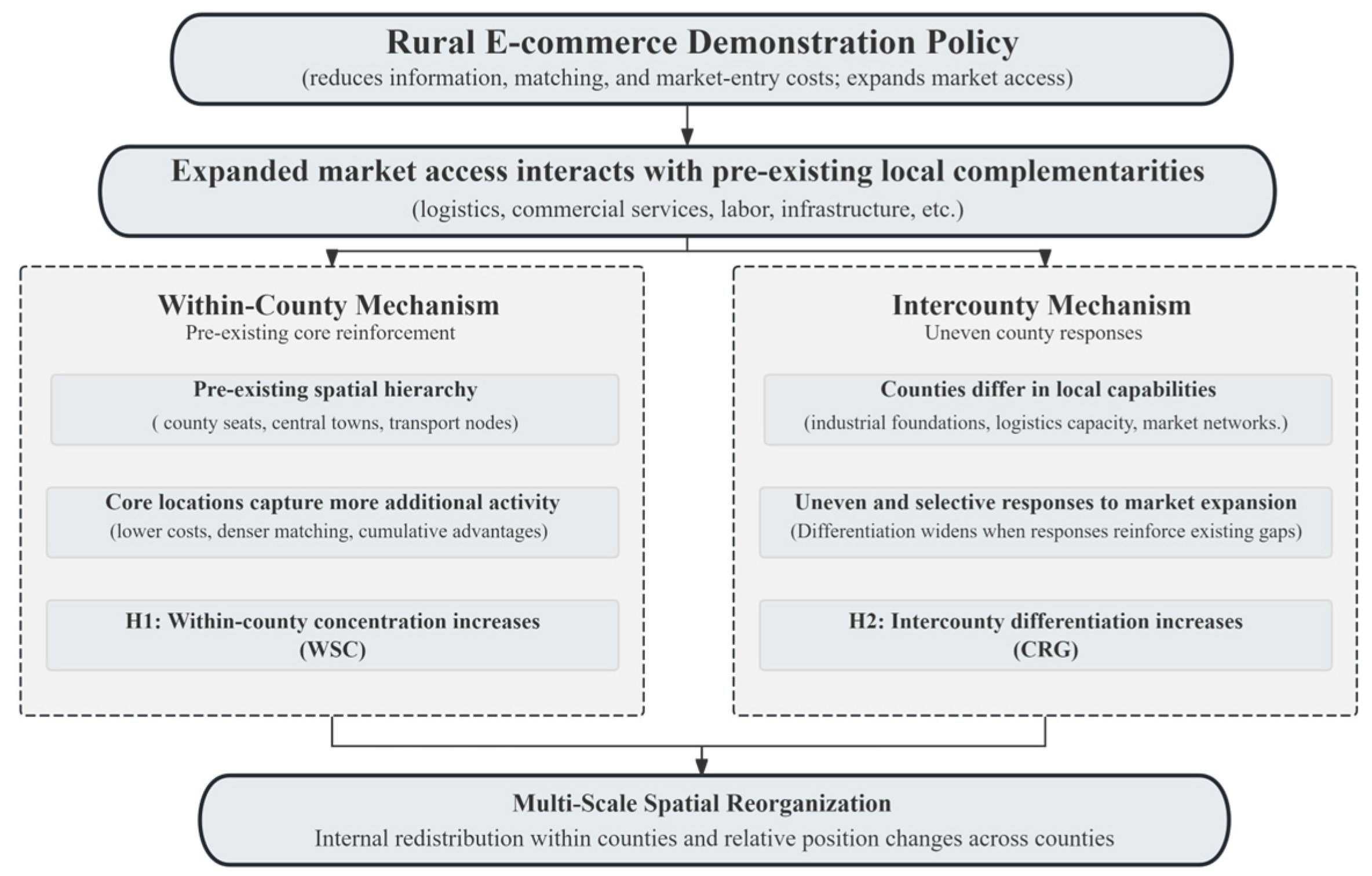
Figure 1 summarizes the proposed theoretical framework, linking the rural e-commerce demonstration program to spatial reorganization at both the within-county and intercounty scales. Within-county spatial concentration (WSC) refers to the concentration of economic activity within a county, whereas the city-relative gap (CRG) measures a county’s deviation from other counties in the same prefecture-level city.

Figure 1. Theoretical framework of multi-scale spatial reorganization under the rural e-commerce demonstration program.

3. Materials and Methods

3.1. Study Area, Policy Rollout, and Sample Construction

This study examines county-level administrative units in China over the period 2011–2024. The Comprehensive Demonstration Program for E-Commerce in Rural Areas was introduced in successive cohorts beginning in 2014, with additional counties entering treatment through 2021. Once a county was designated as a demonstration county, it remained classified as treated in subsequent years, generating staggered variation in policy exposure across counties and over time.

The initial policy–nighttime-light panel covers 2852 counties. Incomplete coverage of county-level socioeconomic controls substantially reduces the number of counties available for analysis. After matching the data sources and applying the sample-selection requirements, the final balanced WSC panel contains 1799 counties and 25,186 county-year observations, including 1222 treated and 577 never-treated counties. Construction of CRG additionally requires at least two other counties with valid nighttime-light measurements within the same prefecture-level city in each year. We exclude 25 counties that fail this requirement in one or more years to maintain a balanced panel. The resulting CRG panel contains 1774 counties and 24,836 county-year observations, including 1200 treated and 574 never-treated counties. Both panels span 2011–2024. The treatment-cohort composition of the two final panels is reported in Appendix C.

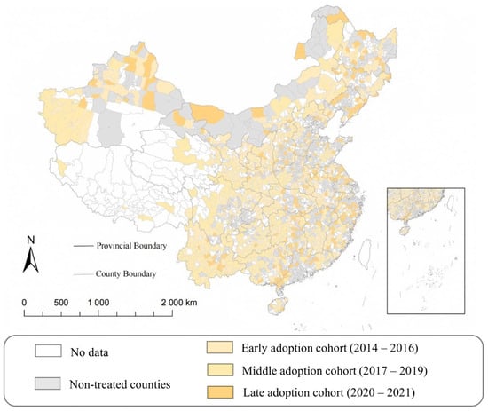
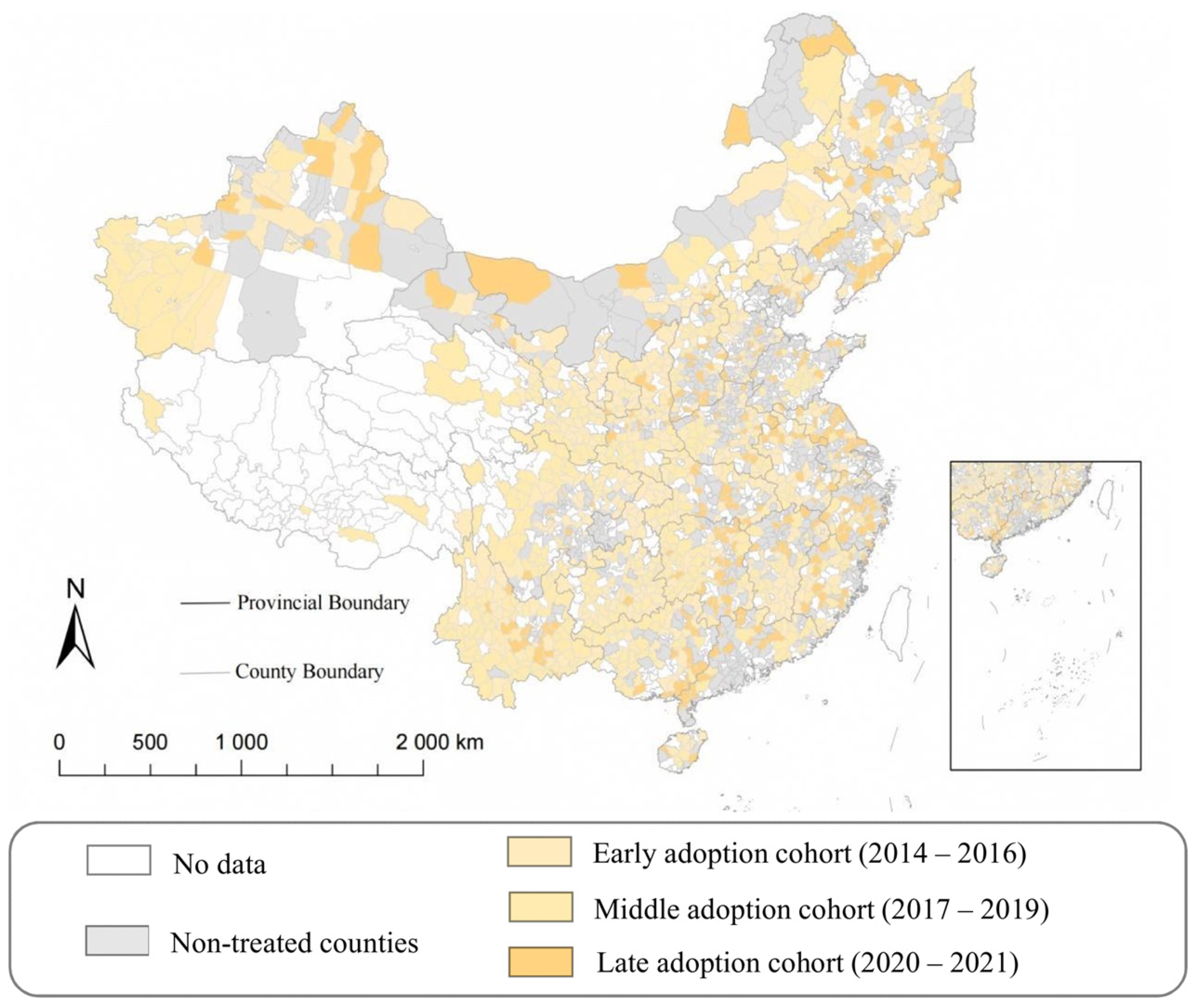
Figure 2 presents the spatial distribution of treated counties and policy-adoption cohorts. For visualization, treatment years are grouped into early (2014–2016), middle (2017–2019), and late (2020–2021) adoption cohorts.

Figure 2. Spatial distribution and adoption cohorts of the Comprehensive Demonstration Program for E-Commerce in Rural Areas.

3.2. Data Sources

The analysis combines four main types of data: policy exposure, nighttime lights, land cover, and county-level socioeconomic statistics. Policy information is compiled from the annual lists of counties selected for the Comprehensive Demonstration Program for E-Commerce in Rural Areas, from which each county’s first treatment year is identified. We use the 2011–2024 observations from the supplied LongNTL annual NPP-VIIRS-like nighttime-light series (NPP denotes the Suomi National Polar-orbiting Partnership satellite; VIIRS denotes the Visible Infrared Imaging Radiometer Suite). The original cross-sensor reconstruction methodology is documented by Chen et al. [23]. According to the accompanying raster metadata, the 2011–2012 observations belong to the reconstructed VIIRS-like segment, whereas observations from 2013 onward belong to the corrected VIIRS segment [24]. Land-cover information is obtained from the China Land Cover Dataset (CLCD), which provides annual land-cover data at a spatial resolution of 30 m [25]. County-level administrative boundary data were obtained from the National Geomatics Center of China (NGCC). We use a fixed set of 2024 county boundaries for all raster-based spatial measurements over 2011–2024, maintaining a consistent geographic framework for nighttime-light and land-cover indicators.

County-level socioeconomic data are mainly drawn from the National Economic and Social Development Statistical Bulletins, the EPS data platform, and the CSMAR database. These sources provide information on population, gross domestic product, value added in the primary sector, local fiscal revenue, and secondary-school enrollment, which are used to construct the control variables described below. The outcome and policy panels were merged with the socioeconomic-control panel using county identifiers and years. Counties were excluded if any required control variable had missing observations at the beginning or end of the study period, or three or more consecutive missing years. Internal gaps of one or two years in the control variables were filled using within-county linear interpolation. No extrapolation was applied to leading or trailing missing observations. Overall, the imputed observations account for less than 5% of the relevant data.

3.3. Variable Definitions

3.3.1. Dependent Variables

(1)

Within-County Spatial Concentration

Nighttime light data provide spatially continuous information on human economic activity and have been widely used to complement conventional socioeconomic statistics, particularly where fine-scale economic data are limited [26]. This study uses the LongNTL annual raster series described in Section 3.2 to characterize the spatial distribution of economic activity within counties. The 30 m annual CLCD impervious-surface layer is converted into a binary mask and aggregated to the nighttime-light grid using average resampling, yielding the impervious-surface fraction within each nighttime-light pixel. This fraction is combined with the pixel’s actual geographic area, accounting for latitude-related variation in pixel size, to construct the developed-area weight defined below. Zero-light observations within developed space are retained as valid observations rather than treated as missing values.

Let y_gct denote the nighttime light intensity of spatial unit g in county c and year t, A_gct denote the effective area of the spatial unit within the county, and s_gct denote the share of the unit classified as impervious surface. The effective impervious-area weight is defined as

w_gct = A_gcts_gct

(1)

The area-weighted mean nighttime light intensity of county c in year t is

$${\bar{y}}_{\mathit{ct}}={\displaystyle \frac{{\displaystyle {\sum }_{g=1}^{n_{\mathit{ct}}}}{w}_{\mathit{gct}}{y}_{\mathit{gct}}}{{\displaystyle {\sum }_{g=1}^{n_{\mathit{ct}}}}{w}_{\mathit{gct}}}}$$

(2)

where n_ct denotes the number of valid spatial units in county c and year t. Following studies that use nighttime-light-based Gini measures to characterize the spatial unevenness of economic activity [27], the within-county spatial concentration index is constructed as

$${\mathrm{WSC}}_{\mathit{ct}}={\displaystyle \frac{{\displaystyle {\sum }_{g=1}^{n_{\mathit{ct}}}}{\displaystyle {\sum }_{j=1}^{n_{\mathit{ct}}}}{w}_{\mathit{gct}}{w}_{\mathit{jct}}\left|y_{\mathit{gct}}-y_{\mathit{jct}}\right|}{2{\bar{y}}_{\mathit{ct}}{\left({\displaystyle {\sum }_{g=1}^{n_{\mathit{ct}}}}{w}_{\mathit{gct}}\right)}^2}}$$

(3)

A larger WSC_ct indicates that nighttime-light-based economic activity is more concentrated in a limited portion of the county’s developed space, whereas a smaller value indicates a more spatially even distribution. Because the weights reflect the actual impervious area represented by each spatial unit, the measure accounts for both differences in nighttime light intensity and differences in developed-space area. Importantly, WSC_ct measures the spatial concentration of economic activity within counties, rather than interpersonal income or welfare inequality.

(2)

Intercounty Differentiation

To measure a county’s relative economic position within its prefecture-level city, this study constructs a city-relative gap based on nighttime light intensity over developed space. The indicator compares each county with the average economic activity of the other counties in the same prefecture-level city and therefore captures intercounty differentiation within a common regional system [28].

For county c in year t, the impervious-area-weighted mean nighttime light intensity is defined as

$${\mathrm{NTL}}_{\mathit{ct}}^{\mathit{imp}}={\displaystyle \frac{{\displaystyle {\sum }_{g=1}^{n_{\mathit{ct}}}}{w}_{\mathit{gct}}{y}_{\mathit{gct}}}{{\displaystyle {\sum }_{g=1}^{n_{\mathit{ct}}}}{w}_{\mathit{gct}}}}$$

(4)

where y_gct denotes nighttime light intensity and w_gct is the effective impervious-area weight defined above. Because nighttime light intensity is right-skewed and may include zero values, the county-level measure is transformed using the inverse hyperbolic sine function [29]:

$$z_{\mathit{ct}}=\mathrm{asinh}\left({\mathrm{NTL}}_{\mathit{ct}}^{\mathit{imp}}\right)$$

(5)

Let county c belong to prefecture-level city p, and let N_pt denote the number of counties with valid observations in city p and year t. To avoid mechanically including the focal county in its own comparison benchmark, a leave-one-out prefecture mean is constructed as

$${\bar{z}}_{-c,\mathit{pt}}={\displaystyle \frac{\sum _{\begin{array}{c}j\in p\\ j\ne c\end{array}}{z}_{\mathit{jt}}}{N_{\mathit{pt}}-1}}$$

(6)

where the benchmark is calculated only when at least three counties within the prefecture-level city have valid observations, that is, N_pt ≥ 3. The city-relative gap is then defined as

$${\mathrm{CRG}}_{\mathit{ct}}=\left|z_{\mathit{ct}}-{\bar{z}}_{-c,\mathit{pt}}\right|$$

(7)

A larger CRG_ct indicates a greater deviation of a county’s nighttime-light-based economic activity from that of other counties in the same prefecture-level city. CRG therefore captures a county’s relative economic differentiation within the prefecture-level system, rather than overall prefecture-level inequality. Because the comparison benchmark is constructed from the contemporaneous outcomes of other counties in the same prefecture-level city, CRG is inherently a relational measure. It may change because of changes in the focal county, changes among its same-city peers, or both. Accordingly, CRG should be interpreted as capturing a county’s relative differentiation within the contemporaneous prefecture-level system, rather than an outcome determined solely by changes in the focal county.

3.3.2. Core Explanatory Variable

The core explanatory variable is county-level exposure to the Comprehensive Demonstration Program for E-Commerce in Rural Areas. Let G_c denote the first year in which county c was designated as a demonstration county. The difference-in-differences (DID) treatment indicator is defined as

DID_ct = 1 (t ≥ G_c)

(8)

where DID_ct = 1 from the first year of policy adoption onward and DID_ct = 0 before adoption. Counties that were never selected as demonstration counties remain untreated throughout the sample period.

3.3.3. Control Variables

To account for observable time-varying county-level socioeconomic conditions that may be associated with both rural e-commerce development and the spatial organization of economic activity, the baseline regressions include a set of socioeconomic controls. Specifically, we control for population density (lnPD), measured as the natural logarithm of population per unit of land area; gross domestic product per capita (lnGDPpc), measured in logarithmic form; primary-sector value added per capita (lnPVApc), also measured in logarithmic form; fiscal revenue per capita (IHSFRpc), transformed using the inverse hyperbolic sine function to accommodate the small number of negative values reported in the original county statistical bulletins; and secondary-school students per 10,000 residents (SS10k) [6,30]. These variables capture differences in local market density, economic development, agricultural conditions, fiscal capacity, and human-capital environment, all of which may influence both a county’s response to e-commerce-related opportunities and the spatial organization of local economic activity.

3.3.4. Pre-Policy Core Areas and Initial Market Density

To examine whether the within-county concentration effect is accompanied by the reinforcement of pre-policy core areas, we construct two indicators of pre-existing core reinforcement. Following the rank-based logic used to identify core spatial structures from nighttime lights [31,32], the identification of core areas is based entirely on pre-policy spatial information. The 2013 impervious-surface footprint defines the fixed developed-space boundary. Before calculating the 2011–2013 mean nighttime-light intensity, the 2011 and 2012 rasters are aligned to the 2013 reference grid using average resampling. Average resampling aligns the grids used for pre-policy pixel ranking; cross-sensor reconstruction and correction are inherited from the supplied LongNTL product. Spatial units within this fixed footprint are ranked in descending order according to their average nighttime light intensity over the pre-policy period 2011–2013. Starting from the highest-intensity units, their 2013 impervious-surface areas are accumulated until 30% of the county’s total 2013 impervious-surface area is reached. If the cutoff falls within a spatial unit, only the share of its developed-area weight required to reach the 30% threshold is assigned to the core, while the remaining share is assigned to the non-core area. Let s_gc ∈ [0,1] denote the share of spatial unit g’s developed-area weight assigned to the core; s_gc = 1 for fully included units, s_gc = 0 for non-core units, and takes a fractional value for the cutoff unit. The same allocation is used in calculating pre-existing core share (CoreShare) and core–non-core light gap (CoreGap). Because both the spatial footprint and the ranking criterion are determined using pre-policy information, the core classification remains fixed throughout the subsequent analysis.

The first indicator is the pre-existing core share (CoreShare):

$${\mathrm{CoreShare}}_{\mathit{ct}}={\displaystyle \frac{\sum _{g\in C_c}{s_{\mathit{gc}}w}_{\mathit{gc}}{y}_{\mathit{gct}}}{\sum _{g\in C_c\cup N{C}_c}{w}_{\mathit{gc}}{y}_{\mathit{gct}}}}$$

(9)

where C_c and NC_c denote the pre-defined core and non-core areas of county c, respectively. A larger value indicates that a greater share of nighttime-light-based economic activity is concentrated in the county’s pre-existing core area.

The second indicator is the core–non-core light gap (CoreGap):

$${\mathrm{CoreGap}}_{\mathit{ct}}=\mathrm{asinh}\left({\overline{\mathrm{NTL}}}_{\mathit{ct}}^{\mathit{core}}\right)-\mathrm{asinh}\left({\overline{\mathrm{NTL}}}_{\mathit{ct}}^{\mathit{noncore}}\right)$$

(10)

where the core and non-core terms denote impervious-area-weighted mean nighttime-light intensity calculated using ${s_{\mathit{gc}}w}_{\mathit{gc}}$ and (1 − s_gc)w_gc, respectively. A larger CoreGap_ct indicates a stronger relative advantage of pre-existing core locations.

To examine whether intercounty differentiation depends on initial local market conditions, we further construct Initial Market Density (IMD). IMD is based on the county-level average log population density over the pre-policy period 2011–2013 and is standardized across counties:

$${\mathrm{IMD}}_c={\displaystyle \frac{{\overline{\ln \mathit{PopDensity}}}_{c,2011-2013}-\mu }{\sigma }}$$

(11)

where μ and σ denote the cross-county mean and standard deviation of the pre-policy measure. Higher values indicate greater pre-policy population density and are interpreted as a proxy for thicker initial local markets [33]. IMD represents initial population concentration, one dimension of local market conditions. Because the measure is constructed entirely from pre-treatment information, it is time-invariant and is not affected by subsequent policy implementation.

3.3.5. Heterogeneity Variables

For the heterogeneity analysis, counties are classified along two spatial dimensions. First, counties are divided into eastern, central, and western China. To maintain a three-region classification, the northeastern provinces of Liaoning, Jilin, and Heilongjiang are included in the eastern region. The regional classification is time-invariant.

Second, Distance to Provincial Capital (DPC) is measured by the geographic distance, in kilometers, from the county government seat to the center of the provincial capital city [34]. Because this measure reflects a county’s fixed geographic position relative to the provincial administrative and economic center, it is time invariant. Counties are divided into near and far groups according to the median of the county-level DPC distribution. Counties with distances below or equal to the median are classified as near the provincial capital, while those above the median are classified as far from the provincial capital.

Table 1 reports summary statistics for the variables used in the empirical analysis. Observation counts vary slightly across variables because of differences in outcome construction and variable-specific data requirements. Throughout the analysis, ln denotes the natural logarithm and IHS denotes the inverse hyperbolic sine transformation.

Table 1. Descriptive Statistics.

Variable	Obs.	Mean	Std. Dev.	Min	Max
WSC	25,186	0.718	0.167	0.000	1.000
CRG	24,836	0.615	0.501	0.000	4.221
DID	25,186	0.362	0.480	0.000	1.000
lnPD	25,186	5.251	1.256	0.140	7.756
lnGDPpc	25,186	10.450	0.711	8.090	14.139
lnPVApc	25,186	8.599	0.595	5.799	11.588
IHSFRpc	25,186	8.225	0.922	−6.839	12.851
SS10k	25,186	477.971	154.829	42.848	2069.345
CoreShare	25,186	0.825	0.150	0.000	1.000
CoreGap	25,186	1.794	0.667	−1.305	4.593
IMD	24,836	0.000	1.000	−4.116	1.965
DPC	25,186	140.878	73.158	2.026	344.077

3.4. Model Construction

To estimate the effect of the rural e-commerce demonstration program on the spatial organization of county-level economic activity, this study exploits the staggered rollout of the policy across counties and employs a two-way fixed-effects difference-in-differences specification:

$$Y_{\mathit{ct}}=\alpha +\beta {\mathrm{DID}}_{\mathit{ct}}+X_{\mathit{ct}}^{\prime }\gamma +{\mu }_c+{\lambda }_t+{\epsilon }_{\mathit{ct}}$$

(12)

where Y_ct denotes the outcome variable for county c in year t. Two outcomes are considered: within-county spatial concentration (WSC_ct) and the city-relative gap (CRG_ct). DID_ct equals one from the year in which county c first enters the rural e-commerce demonstration program and remains one thereafter, and equals zero otherwise. X_ct is a vector of time-varying county-level control variables, including lnPD, lnGDPpc, lnPVApc, IHSFRpc, and SS10k.

Some contemporaneous controls, particularly GDP per capita, primary-sector value added, and fiscal revenue, may themselves respond to policy adoption. We therefore report specifications both with and without these controls in Table 2 and the subsequent analyses. Specifications without contemporaneous controls avoid conditioning on these potentially treatment-affected variables. Coefficients from the controlled specifications are interpreted as conditional estimates, rather than estimates of the total policy effect or separately identified causal direct effects. Both specifications remain subject to the identification assumptions of the research design.

Table 2. Baseline Regression Results.

Dependent Variable	(1)	(2)	(3)	(4)
	WSC	WSC	CRG	CRG
DID	0.0135 *** (0.0022)	0.0108 ***	0.0294 ***	0.0270 ***
		(0.0021)	(0.0085)	(0.0084)
lnPD		−0.0299 ***		−0.0383
		(0.0099)		(0.0446)
lnGDPpc		−0.0151 **		−0.0144
		(0.0066)		(0.0199)
lnPVApc		0.0381 ***		0.0346
		(0.0078)		(0.0239)
IHSFRpc		−0.0144 ***		−0.0199 **
		(0.0027)		(0.0093)
SS10k		−0.000038 ***		−0.000019
		(0.000007)		(0.000037)
Controls	No	Yes	No	Yes
County FE	Yes	Yes	Yes	Yes
Year FE	Yes	Yes	Yes	Yes
N	25,186	25,186	24,836	24,836
Counties	1799	1799	1774	1774
Adj. R2	0.9159	0.9186	0.8078	0.8081

Notes: County-clustered robust standard errors are reported in parentheses. *** and ** denote statistical significance at the 1% and 5% levels, respectively.

County fixed effects, μ_c, absorb time-invariant differences across counties, while year fixed effects, λ_t, control for common macroeconomic and institutional shocks in each year. The coefficient of interest is β, which captures the average change in the corresponding spatial outcome associated with policy implementation, conditional on the included controls and fixed effects. For WSC, this refers to changes in the internal concentration of economic activity within the focal county. For CRG, the estimate captures changes in the focal county’s relative differentiation from its contemporaneous same-city peers under the observed policy rollout. Because the CRG benchmark is itself constructed from peer outcomes, the coefficient should not be interpreted as a pure direct effect that holds other counties’ outcomes fixed.

When cross-county interference is present, the DID coefficient should not be interpreted as an isolated own-county policy effect holding neighboring counties’ treatment status fixed. We therefore examine neighboring treatment exposure and the sensitivity of the estimates to the exclusion of potentially exposed comparison counties.

4. Results

4.1. Descriptive Spatial Patterns

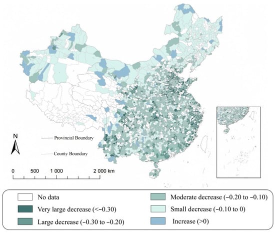
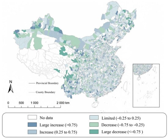
Figure 3 and Figure 4 provide a descriptive overview of long-run changes in the two dimensions of spatial economic organization between 2011 and 2024. Figure 3 maps the change in within-county spatial concentration (WSC), calculated as the 2024 value minus the 2011 value. Declines in WSC are widespread across the sample, although their magnitude varies substantially across counties. Counties experiencing increases in WSC are comparatively limited and spatially dispersed. The map therefore points to considerable geographic heterogeneity within a broader pattern of declining within-county concentration over the study period. This overall decline does not conflict with the positive DID estimate below, which captures the policy-induced deviation from the counterfactual trend rather than the unconditional change in WSC.

Figure 3. Change in within-county spatial concentration (WSC), 2011–2024.

Figure 4. Change in the city-relative gap (CRG), 2011–2024.

Figure 4 presents the corresponding long-run change in the city-relative gap (CRG). In contrast to the more directionally consistent pattern observed for WSC, changes in CRG are more spatially mixed: counties experiencing widening, narrowing, and relatively limited changes coexist across the country. This pattern indicates substantial heterogeneity in the evolution of counties’ relative economic positions within prefecture-level city systems.

4.2. Baseline Regression Results

Table 2 reports the baseline difference-in-differences estimates of the effects of the rural e-commerce demonstration program on within-county spatial concentration and intercounty differentiation. All specifications include county and year fixed effects, with standard errors clustered at the county level.

Columns (1) and (2) report the results for within-county spatial concentration (WSC). The estimated coefficient on DID is 0.0135 without additional controls and is statistically significant at the 1% level. After the baseline controls are included, the coefficient remains positive and statistically significant, with an estimate of 0.0108, equivalent to approximately 0.065 standard deviations of WSC. The results therefore support H1.

Columns (3) and (4) report the corresponding estimates for the city-relative gap (CRG). The coefficient on DID is 0.0294 in the specification without additional controls and 0.0270 after the baseline controls are included, with both estimates statistically significant at the 1% level. The controlled estimate is equivalent to approximately 0.054 standard deviations of CRG. The results therefore indicate that policy implementation is associated with greater county-relative differentiation within the contemporaneous prefecture-level system, providing evidence consistent with H2 within the baseline two-way fixed effects (TWFE) specifications.

The baseline TWFE estimates are positive and statistically significant for both WSC and CRG, with and without contemporaneous socioeconomic controls.

4.3. Parallel-Trends and Placebo Tests

4.3.1. Parallel-Trends Test and Dynamic Effects

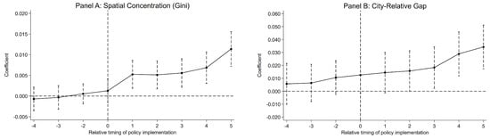
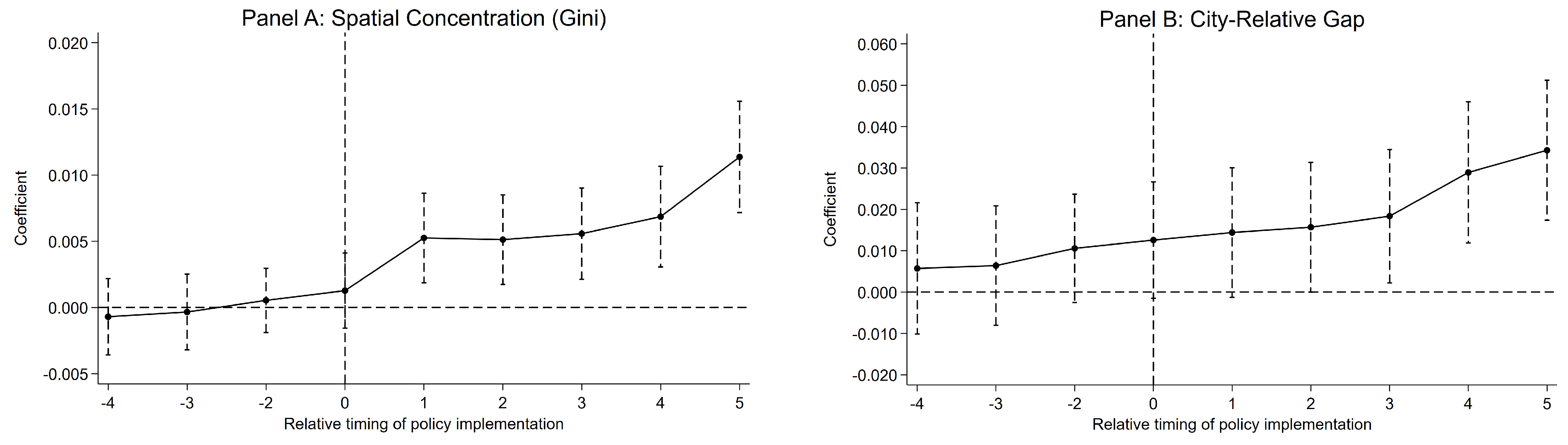
Given the staggered rollout of the rural e-commerce demonstration program, we employ the interaction-weighted event-study estimator of Sun and Abraham to examine pre-treatment trends and the dynamic evolution of the policy effects [35]. The year immediately preceding policy adoption (t = −1) serves as the reference period, and Figure 5 reports estimates from four years before to five years after treatment.

Figure 5. Sun–Abraham event-study estimates for WSC and CRG. The horizontal dashed line indicates zero, and the vertical dashed line marks the year of policy implementation (event time 0).

As shown in Figure 5, there is no evidence of differential pre-treatment trends for either outcome. The joint test of the coefficients at t = −4, −3, −2 yields a p-value of 0.869 for WSC and 0.443 for CRG. In both cases, the null hypothesis that the pre-treatment coefficients are jointly equal to zero cannot be rejected. These results are consistent with, although they do not establish, the parallel-trends assumption.

The post-treatment estimates indicate that the spatial effects emerge gradually. For WSC, the coefficient in the year of policy adoption is small and statistically insignificant, but becomes positive and significant from the first post-treatment year onward and reaches approximately 0.0114 by t = 5. For CRG, the post-treatment coefficients are also positive and increase over time, reaching approximately 0.0343 by t = 5. These dynamic patterns indicate progressively stronger post-treatment increases in within-county concentration, while counties also become increasingly differentiated from their contemporaneous same-city peers over event time.

4.3.2. Placebo Test

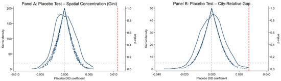
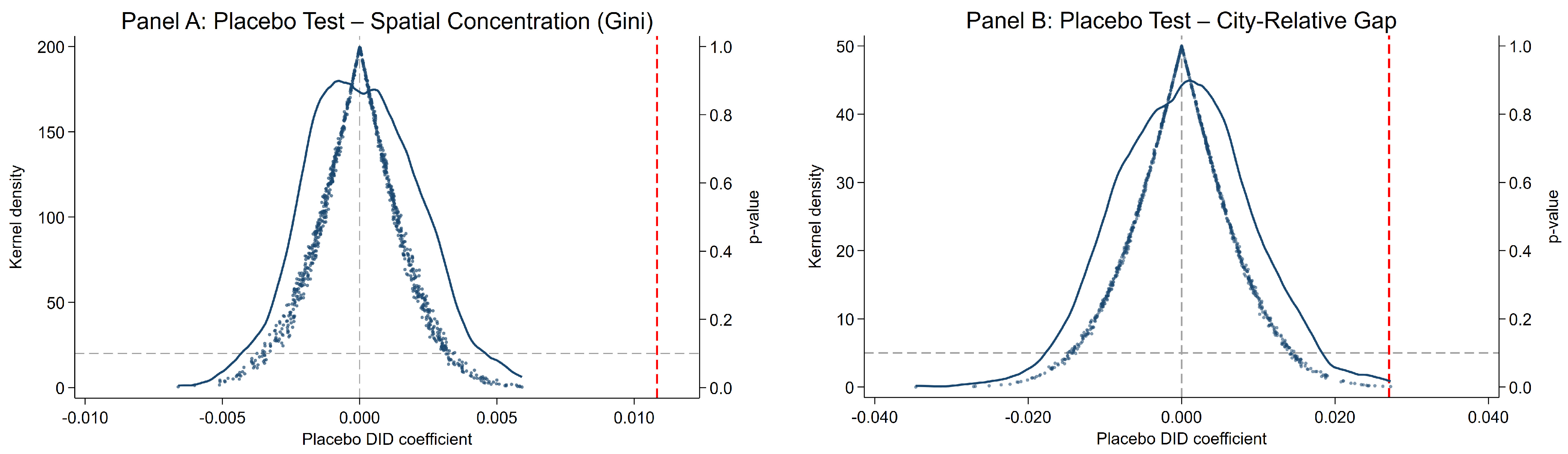
To assess whether the baseline estimates could plausibly arise under randomized treatment assignment, we conduct a randomization-based placebo test. Treatment status and treatment cohorts are randomly reassigned across counties 1000 times while preserving the number of treated and never-treated counties and the size of each treatment cohort. For each placebo assignment, the baseline DID specification is re-estimated using the same controls and fixed effects.

Figure 6 presents the distributions of the placebo estimates. For both outcomes, the placebo estimates are centered around zero, while the observed estimates lie in the extreme right tails of the placebo distributions. The corresponding empirical two-sided p-values are approximately 0.001 for WSC and 0.004 for CRG.

Figure 6. Randomization-based placebo tests for WSC and CRG. The gray vertical dashed line indicates a zero placebo coefficient, the red vertical dashed line indicates the observed DID estimate, and the gray horizontal dashed line marks the p-value reference threshold of 0.10.

Overall, the placebo results indicate that the baseline estimates are unlikely to be generated by random reassignment of treatment status and timing.

4.4. Robustness Checks

Table 3 reports a series of robustness checks addressing province-specific time-varying shocks, treatment-cohort and sample composition, inference, and changes in the spatial extent of developed land.

Table 3. Robustness Checks.

	(1) Province-Year FE	(2) Drop 2014 Cohort	(3) Prefecture Clustering	(4) Fixed 2013 Built-up Space	(5) Callaway–Sant’Anna ATT
Within-County Spatial Concentration (WSC)
Effect estimate	0.0049 **	0.0111 ***	0.0108 ***	0.0121 ***	0.0133 ***
Standard error	(0.0023)	(0.0022)	(0.0024)	(0.0018)	(0.0026)
N	25,186	24,444	25,186	25,186	25,186
Counties	1799	1746	1799	1799	1799
Adj. R2	0.9313	0.9180	0.9186	0.9286	—
City-Relative Gap (CRG)
Effect estimate	0.0225 **	0.0269 ***	0.0270 ***	—	0.0176 *
Standard error	(0.0087)	(0.0087)	(0.0094)	—	(0.0093)
N	24,836	24,108	24,836	—	24,836
Counties	1774	1722	1774	—	1774
Adj. R2	0.8136	0.8081	0.8081	—	—
Controls	Yes	Yes	Yes	Yes	No
County FE	Yes	Yes	Yes	Yes	—
Year FE	Absorbed	Yes	Yes	Yes	—
Province-Year FE	Yes	No	No	No	—
Cluster level	County	County	Prefecture	County	County (bootstrap)

Notes: Clustered standard errors are reported in parentheses. ***, **, and * denote statistical significance at the 1%, 5%, and 10% levels, respectively. The Callaway–Sant’Anna estimates use never-treated counties as the comparison group and are estimated without covariates; inference is based on 999 county-clustered bootstrap replications.

Column (1) introduces province-by-year fixed effects. The estimated coefficients remain positive and statistically significant for WSC (0.0049) and CRG (0.0225). However, the WSC estimate decreases by approximately 55% relative to the controlled baseline estimate of 0.0108. This attenuation indicates that the estimated magnitude is sensitive to adjustment for province-specific time-varying factors, despite the persistence of a statistically significant positive coefficient.

Columns (2) and (3) examine the sensitivity of the results to treatment-cohort composition and the level of statistical inference. The estimates also remain positive and statistically significant after excluding the 2014 treatment cohort and when standard errors are clustered at the prefecture level.

Column (4) addresses the possibility that changes in WSC mechanically reflect changes in the spatial extent of developed land. We reconstruct WSC using the 2013 impervious-surface footprint fixed throughout the sample period. The estimated coefficient remains positive and highly significant at 0.0121, showing that the concentration effect persists when the developed-space boundary is held constant.

Finally, Column (5) re-estimates the average treatment effects using the Callaway–Sant’Anna estimator to account for heterogeneous treatment effects under staggered policy adoption [36]. We report the unconditional specification without covariates as an alternative staggered-adoption estimator, rather than conditioning on socioeconomic variables that may themselves evolve with policy exposure. Using never-treated counties as the comparison group, the Callaway–Sant’Anna estimator yields an ATT of 0.0133 for WSC, close to the uncontrolled TWFE estimate of 0.0135. For CRG, the corresponding ATT is 0.0176, smaller than the TWFE estimates and not statistically significant at the 5% level (p = 0.059). Although its sign agrees with the baseline result, this does not establish comparable robustness in magnitude or statistical precision. Overall, the reported specifications provide stronger support for within-county concentration than for intercounty differentiation, with the evidence for H2 remaining suggestive and estimator-sensitive.

We examine cross-county interference using two complementary exercises. First, we augment the baseline specification with a time-varying indicator of treatment exposure through Queen-contiguous neighboring counties. The own-county DID coefficients remain positive and statistically significant for both WSC and CRG, while neighboring exposure is also positively associated with both outcomes. Second, we exclude never-treated comparison counties bordering any county that adopted the program during the study period. The resulting DID estimates remain positive and statistically significant, at 0.0039 for WSC and 0.0207 for CRG, although their magnitudes decline, particularly for WSC. Thus, positive policy coefficients persist when potentially neighbor-exposed comparison counties are excluded. The exclusion estimates refer to the remaining nonadjacent comparison counties; the smaller comparison group changes the basis of comparison and limits extrapolation beyond this restricted sample. Appendix B reports the exposure definition, corresponding estimates, and sample sizes.

5. Further Analyses

5.1. Reinforcement of Pre-Existing Core Locations

To examine whether the increase in within-county spatial concentration is accompanied by a strengthening of pre-existing core locations, we examine two complementary measures, Pre-existing Core Share (CoreShare) and Core–Non-Core Light Gap (CoreGap), based on the pre-policy core classification defined in Section 3.3.4. Table 4 reports the results.

Table 4. Reinforcement of Pre-Existing Core Locations.

Dependent Variable	(1)	(2)	(3)	(4)
	CoreShare	CoreShare	CoreGap	CoreGap
DID	0.0103 ***	0.0077 ***	0.0911 ***	0.0881 ***
	(0.0021)	(0.0020)	(0.0124)	(0.0123)
Controls	No	Yes	No	Yes
County FE	Yes	Yes	Yes	Yes
Year FE	Yes	Yes	Yes	Yes
N	25,186	25,186	25,186	25,186
Counties	1799	1799	1799	1799

Note: County-clustered robust standard errors are reported in parentheses. *** denotes statistical significance at the 1% level.

Columns (1) and (2) report DID coefficients of 0.0103 and 0.0077 for CoreShare, respectively, corresponding to increases of approximately 1.03 and 0.77 percentage points in the nighttime-light share accounted for by pre-policy core areas. Columns (3) and (4) report coefficients of 0.0911 and 0.0881 for CoreGap. All four estimates are positive and statistically significant at the 1% level. Together, these findings associate policy adoption with a larger nighttime-light share and a greater relative nighttime-light intensity advantage for pre-existing core areas within the fixed developed-space footprint.

The two results jointly sharpen the interpretation of the baseline WSC effect. The increase in spatial concentration is accompanied by a strengthening of locations that were already economically dominant before policy adoption, rather than arising from an arbitrary redistribution of activity across developed space. Because both the core classification and the underlying spatial footprint are fixed using pre-policy information, this pattern cannot be mechanically generated by post-treatment reclassification of core locations. The findings are therefore consistent with the reinforcement of pre-existing spatial advantages. Logistics, commercial services, and infrastructure may contribute to this pattern, although their individual roles are not directly identified here [9]. These indicators capture relative core reinforcement rather than absolute changes in economic activity outside the core.

As a sensitivity check, we redefine pre-existing core areas using a more restrictive 20% developed-space threshold. The estimated effects on CoreShare and CoreGap remain positive and statistically significant, indicating that the core-reinforcement result is not driven by the baseline 30% cutoff (see Appendix A).

5.2. Initial Market Density (IMD) and Intercounty Differentiation

The baseline CRG results indicate greater county-relative differentiation following policy implementation. To examine whether this effect varies with pre-existing local market conditions, we interact DID with initial market density (IMD). Columns (3) and (4) further interact the continuous IMD measure with year indicators, allowing the association between initial market density and CRG to vary flexibly across years. Table 5 reports the results.

Table 5. Moderating Effect of Initial Market Density (IMD).

Panel A. Interaction specifications.
Dependent Variable	(1)	(2)	(3)	(4)
	CRG	CRG	CRG	CRG
DID	0.0220 *** (0.0082)	0.0218 *** (0.0082)	0.0174 ** (0.0083)	0.0190 ** (0.0084)
DID × IMD	−0.0579 *** (0.0099)	−0.0562 *** (0.0100)	−0.0248 ** (0.0104)	−0.0252 ** (0.0103)
Controls	No	Yes	No	Yes
County FE	Yes	Yes	Yes	Yes
Year FE	Yes	Yes	Yes	Yes
IMD × Year interactions	No	No	Yes	Yes
N	24,836	24,836	24,836	24,836
Counties	1774	1774	1774	1774
Panel B. Conditional DID effects from Column (4).
IMD level	Conditional DID Estimate	SE	p-Value	95% CI
−1 SD	0.0442	0.0149	0.003	[0.0150, 0.0733]
Mean	0.0190	0.0084	0.024	[0.0025, 0.0354]
+1 SD	−0.0062	0.0115	0.590	[−0.0288, 0.0164]

Note: County-clustered robust standard errors are reported in parentheses. *** and ** denote statistical significance at the 1% and 5% levels, respectively. Conditional DID effects are calculated as linear combinations of the DID and DID × IMD coefficients from Column (4) of Panel A. Standard errors and 95% confidence intervals are computed using the county-clustered variance–covariance matrix, including the covariance between these coefficients. Mean corresponds to IMD = 0; −1 SD and +1 SD correspond to IMD = −1 and IMD = +1, respectively. Abbreviations: SE = standard error; CI = confidence interval; SD = standard deviation.

The DID × IMD coefficient is negative across all four specifications. In Column (4) of Panel A, the coefficient is −0.0252 (p = 0.015), indicating that the conditional DID estimate decreases by approximately 0.0252 for a one-standard-deviation increase in pre-policy population density. The implied conditional effect is approximately 0.0190–0.0252 × IMD, with its point estimate crossing zero at about 0.75 standard deviations above mean IMD.

Panel B reports the conditional DID estimates from Column (4). The estimates are positive and statistically significant at IMD = −1 and IMD = 0. At IMD = +1, the estimate is −0.0062 (p = 0.590; 95% confidence interval: −0.0288 to 0.0164). The high-density point estimate is negative, with a confidence interval that includes zero.

This density-related gradient complements the average CRG estimates by showing how the estimated response varies with pre-policy population concentration.

5.3. Regional and Locational Heterogeneity

We further examine whether the spatial effects of rural e-commerce vary across broader geographic contexts. Following the classifications defined in Section 3.3.5, the analysis considers regional location and distance to the provincial capital (DPC). Table 6 reports the estimates, and cross-group differences are evaluated using Wald tests.

Table 6. Regional and Locational Heterogeneity.

Group/Test	(1)	(2)	(3)	(4)
	WSC	WSC	CRG	CRG
Regional Heterogeneity
East	0.0160 *** (0.0035)	0.0158 *** (0.0031)	0.0098 (0.0141)	0.0126 (0.0137)
Central	0.0043 (0.0028)	0.0039 (0.0027)	0.0261 * (0.0138)	0.0257 * (0.0136)
West	0.0021 (0.0044)	0.0027 (0.0042)	0.0282 * (0.0156)	0.0277 * (0.0158)
Wald p-value: East = Central	0.0096	0.0142	0.4090	0.3707
Wald p-value: East = West	0.0140	0.0113	0.3813	0.3830
Wald p-value: Central = West	0.6720	0.5561	0.9196	0.9733
Distance to Provincial Capital
Near provincial capital	0.0191 *** (0.0028)	0.0154 *** (0.0027)	0.0433 *** (0.0132)	0.0387 *** (0.0132)
Far from provincial capital	0.0052 (0.0035)	0.0042 (0.0033)	0.0089 (0.0109)	0.0084 (0.0108)
Wald p-value: Near = Far	0.0019	0.0080	0.0447	0.0617
Controls	No	Yes	No	Yes
County FE	Yes	Yes	Yes	Yes
Year FE	Yes	Yes	Yes	Yes

Note: Cross-group p-values are obtained from Wald tests of equality of treatment effects based on pooled interaction specifications. County-clustered robust standard errors are reported in parentheses. *** and * denote statistical significance at the 1% and 10% levels, respectively.

Regional heterogeneity is clearer for WSC than for CRG. The WSC coefficient in eastern counties is 0.0160 in Column (1) and 0.0158 in Column (2). Both exceed the corresponding central and western estimates, with Wald p-values of 0.0096 and 0.0140 in Column (1), and 0.0142 and 0.0113 in Column (2). The central–western difference is not statistically significant in either specification. For CRG, none of the cross-regional differences is statistically significant.

For distance to the provincial capital, the WSC coefficients for near and far counties are 0.0191 and 0.0052 in Column (1), compared with 0.0154 and 0.0042 in Column (2). The near–far difference is statistically significant in both specifications, with Wald p-values of 0.0019 and 0.0080, respectively. For CRG, the corresponding coefficients are 0.0433 and 0.0089 in Column (3), and 0.0387 and 0.0084 in Column (4). The near–far difference is significant at the 5% level in Column (3) and at the 10% level in Column (4), with p-values of 0.0447 and 0.0617, respectively.

Overall, geographic heterogeneity is more systematic for within-county concentration than for county-relative differentiation. WSC differs significantly across regional locations and proximity to provincial capitals, whereas the geographic variation in CRG is primarily associated with proximity to provincial capitals.

6. Discussion

6.1. Digital Market Expansion and Spatial Differentiation

The results show that improved market access can be accompanied by increasing spatial differentiation. Rural e-commerce may expand economic opportunities without distributing the associated activity evenly across locations, both within counties and across counties embedded in the same regional system.

This distinction helps reconcile market integration with increasing spatial differentiation. E-commerce lowers information, matching, and market-entry frictions, but it does not remove the location dependence of logistics, warehousing, distribution, labor, and business services [37]. The expansion of accessible markets can therefore increase the returns to economic activity while leaving important agglomeration forces intact [38]. The persistence of the concentration effect within a fixed developed-space boundary, together with the strengthening of pre-existing core locations, is consistent with this interpretation [12]. This finding complements Yu et al.’s evidence that the rural e-commerce demonstration policy reduces within-county dispersion in nighttime lights, measured by the standard deviation of nighttime-light intensity [8], by showing that different spatial margins of county development can evolve differently.

The same principle extends to the intercounty scale. A common improvement in market access need not produce convergence when counties differ in their capacity to translate new opportunities into local economic activity [39,40]. The positive baseline TWFE CRG estimates suggest wider absolute gaps in counties’ relative positions within the contemporaneous prefecture-level system under the observed policy rollout, although support for this interpretation varies across estimators. This county-relative evidence complements prefecture-wide inequality analyses by showing how individual counties’ positions change within a common regional system [41]. More generally, market integration and spatial convergence are analytically distinct processes: digitalization can broaden economic opportunities while making their spatial realization more differentiated [38].

6.2. Pre-Existing Conditions and Uneven Spatial Adjustment

Further analyses indicate that the spatial response to rural e-commerce is shaped by conditions established before policy implementation. Within counties, pre-existing core areas gain both a larger share of economic activity and a stronger nighttime-light advantage over non-core developed space. This pattern is consistent with cumulative spatial advantage: established locations may be better positioned to absorb additional activity associated with digital market expansion [42]. The results therefore point to a reinforcement of pre-existing spatial advantages within the fixed developed-space footprint.

Across counties, the estimated CRG response declines with pre-policy population density. The pattern links county-relative adjustment to conditions established before policy adoption. The conditional estimates are positive at low and mean IMD, whereas the estimate at IMD = +1 is negative but statistically indistinguishable from zero. Differences in demand, firms, and service networks may offer possible explanations for density-related variation in the estimated response [2,43].

The geographic heterogeneity results further suggest that these conditioning factors are scale-specific. Regional location and proximity to provincial capitals are clearly associated with differences in the WSC effect, whereas the corresponding variation in CRG is much less systematic. Taken together, the evidence indicates that pre-existing spatial and market conditions remain important for the geography of rural digitalization, but their relevance differs between within-county concentration and intercounty differentiation.

6.3. Limitations and Future Research

Several limitations define the scope of these findings. First, nighttime lights provide a spatially detailed proxy for economic activity rather than direct measures of output, employment, income, or welfare. Residual cross-sensor differences in spatial resolution, background noise, and low-intensity sensitivity may affect WSC and the 2011–2013 core classification. Future research using geocoded firm, employment, logistics, or transaction data could clarify the activities underlying these spatial changes.

Second, CRG measures the absolute deviation of a county from its prefecture-level peers. It therefore captures relative differentiation but does not reveal whether a county moves above or below the peer benchmark, nor whether overall prefecture-level inequality increases. In addition, because the benchmark is constructed from the contemporaneous outcomes of other counties, it may itself change when peer counties are affected by the rural e-commerce program. The CRG estimates should therefore be interpreted as changes in county-relative differentiation under the observed policy rollout, rather than as pure direct own-county effects holding peer outcomes fixed. Future research could complement this measure with directional indicators or benchmarks constructed from stable untreated peers.

Third, data availability and administrative comparability limit the coverage of the analysis. Missing county-level socioeconomic controls, together with the other sample-selection requirements, restrict the analytical samples to a subset of counties. The findings therefore apply to the retained samples and may not generalize to all counties in China. Using fixed 2024 county boundaries provides a consistent geographic framework for measuring nighttime lights and developed space throughout the study period. However, this spatial consistency does not by itself ensure that historical socioeconomic statistics and policy designations are fully comparable across administrative changes. Potential discrepancies between historical reporting units and the reference geography remain a limitation. Future research could improve coverage and comparability through more complete county-level statistics and explicit historical administrative crosswalks.

Finally, the pre-existing core, IMD, and neighboring-exposure analyses describe spatial patterns associated with the program. Direct data on logistics facilities, firm locations, supply-chain links, and intercounty flows would help distinguish the underlying channels.

7. Conclusions and Policy Implications

7.1. Conclusions

Using county-level panel data from 2011 to 2024, this study examines how China’s rural e-commerce demonstration program changes the spatial distribution of economic activity within counties and the relative positions of counties within prefecture-level cities. The positive WSC association persists across the reported specifications, although its estimated magnitude is smaller after including province-by-year fixed effects. Evidence of greater county-relative differentiation is less consistent across estimators.

Further analyses clarify the spatial patterns underlying these effects. Within counties, the concentration effect remains when developed space is fixed at its pre-policy footprint, and the share of nighttime light accounted for by pre-policy core areas within this fixed footprint increases by approximately 0.77 percentage points. At the intercounty scale, the CRG response is weaker in counties with higher initial market density, while the WSC effect is stronger in eastern counties and in counties closer to provincial capitals. These findings provide stronger evidence of greater concentration within developed space than of wider differences in counties’ relative positions within contemporaneous prefecture-level systems. The results therefore add a spatial-distributional dimension to assessments of rural e-commerce policies that focus primarily on aggregate county-level outcomes.

7.2. Policy Implications

First, rural e-commerce policy should complement county-level digital platforms with stronger connections between established economic cores and surrounding towns and rural communities. The observed reinforcement of pre-existing core locations suggests that new market opportunities are more readily absorbed where commercial and service capacity is already concentrated. Policy can improve access to these nodes through township-level logistics services, shared warehousing and distribution facilities, and stronger connections between county centers and surrounding areas. This would allow a wider set of locations to participate in the market opportunities generated by rural e-commerce.

Second, complementary support should be differentiated according to counties’ initial market conditions. The stronger intercounty differentiation observed in initially thinner markets suggests that basic local capabilities remain important for translating digital market access into economic activity. Complementary resources should therefore be adapted to local conditions, with specific priorities for logistics, warehousing, business services, or other support determined by local needs and infrastructure gaps. Policy evaluation could also incorporate spatial indicators that track how economic activity is distributed within counties and how counties’ relative positions within prefecture-level cities evolve over time.

References

- Goldfarb, A.; Tucker, C. Digital Economics. J. Econ. Lit. 2019, 57, 3–43. [Google Scholar] [CrossRef] [Scilit]
- Couture, V.; Faber, B.; Gu, Y.; Liu, L. Connecting the Countryside via E-Commerce: Evidence from China. Am. Econ. Rev. Insights 2021, 3, 35–50. [Google Scholar] [CrossRef] [Scilit]
- Qin, Q.; Guo, H.; Shi, X.; Chen, K. Rural E-commerce and County Economic Development in China. China World Econ. 2023, 31, 26–60. [Google Scholar] [CrossRef] [Scilit]
- Li, G.; Qin, J. Income Effect of Rural E-Commerce: Empirical Evidence from Taobao Villages in China. J. Rural Stud. 2022, 96, 129–140. [Google Scholar] [CrossRef] [Scilit]
- Wei, Y.D.; Lin, J.; Zhang, L. E-Commerce, Taobao Villages and Regional Development in China. Geogr. Rev. 2020, 110, 380–405. [Google Scholar] [CrossRef] [Scilit]
- Liu, Y.; Zhou, M. Can Rural E-Commerce Narrow the Urban–Rural Income Gap? Evidence from Coverage of Taobao Villages in China. China Agric. Econ. Rev. 2023, 15, 580–603. [Google Scholar] [CrossRef] [Scilit]
- Lu, Z.; Wang, S. The Sword Effect of Electronic Informatization on Income Inequality: E-Commerce and E-Government. J. Theor. Appl. Electron. Commer. Res. 2026, 21, 56. [Google Scholar] [CrossRef] [Scilit]
- Yu, Y.; Tu, H.; Tian, Q. The Impacts of Rural E-Commerce on County Economic Development: Evidence from National Rural E-Commerce Comprehensive Demonstration Policy in China. J. Theor. Appl. Electron. Commer. Res. 2025, 20, 235. [Google Scholar] [CrossRef] [Scilit]
- Zhao, Z.; Liu, R.; Wang, Q. Place-Based Polices and e-Commerce Development in Rural China. China Econ. Rev. 2024, 83, 102085. [Google Scholar] [CrossRef] [Scilit]
- Heitz, A.; Launay, P.; Beziat, A. Heterogeneity of Logistics Facilities: An Issue for a Better Understanding and Planning of the Location of Logistics Facilities. Eur. Transp. Res. Rev. 2019, 11, 5. [Google Scholar] [CrossRef] [Scilit]
- Wang, C.; Zhou, T.; Ren, M. Driving Spatial Network Connections in Rural Settlements: The Role of e-Commerce. Appl. Geogr. 2023, 159, 103067. [Google Scholar] [CrossRef] [Scilit]
- Goldmanis, M.; Hortaçsu, A.; Syverson, C.; Emre, Ö. E-Commerce and the Market Structure of Retail Industries. Econ. J. 2010, 120, 651–682. [Google Scholar] [CrossRef] [Scilit]
- Redding, S.J.; Turner, M.A. Transportation Costs and the Spatial Organization of Economic Activity. In Handbook of Regional and Urban Economics; Duranton, G., Henderson, J.V., Strange, W.C., Eds.; Elsevier: Amsterdam, The Netherlands, 2015; Volume 5, pp. 1339–1398. [Google Scholar] [CrossRef] [Scilit]
- Cui, J.; Luo, J.; Kong, X.; Sun, J.; Gu, J. Characterising the Hierarchical Structure of Urban-Rural System at County Level Using a Method Based on Interconnection Analysis. J. Rural Stud. 2022, 93, 263–272. [Google Scholar] [CrossRef] [Scilit]
- McCann, B.T.; Folta, T.B. Demand- and Supply-Side Agglomerations: Distinguishing between Fundamentally Different Manifestations of Geographic Concentration. J. Manag. Stud. 2009, 46, 362–392. [Google Scholar] [CrossRef] [Scilit]
- Porter, M.E. Location, Competition, and Economic Development: Local Clusters in a Global Economy. Econ. Dev. Q. 2000, 14, 15–34. [Google Scholar] [CrossRef] [Scilit]
- Duranton, G.; Puga, D. The Economics of Urban Density. J. Econ. Perspect. 2020, 34, 3–26. [Google Scholar] [CrossRef] [Scilit]
- Krugman, P. Increasing Returns and Economic Geography. J. Polit. Econ. 1991, 99, 483–499. [Google Scholar] [CrossRef] [Scilit] [PubMed]
- Gennaioli, N.; La Porta, R.; Lopez-de-Silanes, F.; Shleifer, A. Human Capital and Regional Development. Q. J. Econ. 2013, 128, 105–164. [Google Scholar] [CrossRef] [Scilit]
- Holl, A.; Rama, R. Spatial Patterns and Drivers of SME Digitalisation. J. Knowl. Econ. 2023, 15, 5625–5649. [Google Scholar] [CrossRef] [Scilit] [PubMed]
- Kline, P.; Moretti, E. People, Places, and Public Policy: Some Simple Welfare Economics of Local Economic Development Programs. Annu. Rev. Econ. 2014, 6, 629–662. [Google Scholar] [CrossRef] [Scilit]
- Miyauchi, Y. Matching and Agglomeration: Theory and Evidence From Japanese Firm-to-Firm Trade. Econometrica 2024, 92, 1869–1905. [Google Scholar] [CrossRef] [Scilit]
- Chen, Z.; Yu, B.; Yang, C.; Zhou, Y.; Yao, S.; Qian, X.; Wang, C.; Wu, B.; Wu, J. An Extended Time Series (2000–2018) of Global NPP-VIIRS-like Nighttime Light Data from a Cross-Sensor Calibration. Earth Syst. Sci. Data 2021, 13, 889–906. [Google Scholar] [CrossRef] [Scilit]
- Elvidge, C.D.; Zhizhin, M.; Ghosh, T.; Hsu, F.-C.; Taneja, J. Annual Time Series of Global VIIRS Nighttime Lights Derived from Monthly Averages: 2012 to 2019. Remote Sens. 2021, 13, 922. [Google Scholar] [CrossRef] [Scilit]
- Yang, J.; Huang, X. The 30 m Annual Land Cover Datasets and Its Dynamics in China from 1985 to 2025. Earth Syst. Sci. 2026, 13, 3907–3925. [Google Scholar] [CrossRef]
- Henderson, J.V.; Storeygard, A.; Weil, D.N. Measuring Economic Growth from Outer Space. Am. Econ. Rev. 2012, 102, 994–1028. [Google Scholar] [CrossRef] [Scilit] [PubMed]
- Ivan, K.; Holobâcă, I.-H.; Benedek, J.; Török, I. Potential of Night-Time Lights to Measure Regional Inequality. Remote Sens. 2019, 12, 33. [Google Scholar] [CrossRef] [Scilit]
- Jean, N.; Burke, M.; Xie, M.; Davis, W.M.; Lobell, D.B.; Ermon, S. Combining Satellite Imagery and Machine Learning to Predict Poverty. Science 2016, 353, 790–794. [Google Scholar] [CrossRef] [Scilit] [PubMed]
- Bellemare, M.F.; Wichman, C.J. Elasticities and the Inverse Hyperbolic Sine Transformation. Oxf. Bull. Econ. Stat. 2020, 82, 50–61. [Google Scholar] [CrossRef] [Scilit]
- Zhang, Y.; Long, H.; Ma, L.; Tu, S.; Li, Y.; Ge, D. Analysis of Rural Economic Restructuring Driven by E-Commerce Based on the Space of Flows: The Case of Xiaying Village in Central China. J. Rural Stud. 2022, 93, 196–209. [Google Scholar] [CrossRef] [Scilit]
- Huang, Y.; Wu, C.; Chen, M.; Yang, J.; Ren, H. A Quantile Approach for Retrieving the “Core Urban-Suburban-Rural” (USR) Structure Based on Nighttime Light. Remote Sens. 2020, 12, 4179. [Google Scholar] [CrossRef] [Scilit]
- Huang, Y.; Yang, J.; Chen, M.; Wu, C.; Ren, H.; Liu, Y. An Approach for Retrieving Consistent Time Series “Urban Core–Suburban-Rural” (USR) Structure Using Nighttime Light Data from DMSP/OLS and NPP/VIIRS. Remote Sens. 2022, 14, 3642. [Google Scholar] [CrossRef] [Scilit]
- Bleakley, H.; Lin, J. Thick-Market Effects and Churning in the Labor Market: Evidence from U.S. Cities. J. Urban Econ. 2012, 72, 87. [Google Scholar] [CrossRef] [Scilit] [PubMed]
- Wang, Z.; Xu, J.; Fang, C.; Xu, L.; Qi, Y. The Study on County Accessibility in China: Characteristics and Effects on Population Agglomeration. J. Geogr. Sci. 2011, 21, 18–34. [Google Scholar] [CrossRef] [Scilit]
- Sun, L.; Abraham, S. Estimating Dynamic Treatment Effects in Event Studies with Heterogeneous Treatment Effects. J. Econom. 2021, 225, 175–199. [Google Scholar] [CrossRef] [Scilit]
- Callaway, B.; Sant’Anna, P.H.C. Difference-in-Differences with Multiple Time Periods. J. Econom. 2021, 225, 200–230. [Google Scholar] [CrossRef] [Scilit]
- Cui, X.; Huang, W.; Zhang, J.; Deng, W. Exploring the Spatiotemporal Evolution Mechanism of Rural E-Commerce: Insights from the Experience of Taobao Towns in China. Humanit. Soc. Sci. Commun. 2024, 11, 789. [Google Scholar] [CrossRef] [Scilit]
- Aiba, I. Information Technology, Market Congestion, and Economic Geography. Ann. Reg. Sci. 2024, 73, 1269–1295. [Google Scholar] [CrossRef] [Scilit]
- Zhang, C.; Zhao, S. Selective but Productive: How Does an e-Commerce Expansion Policy Affect Rural Economic Vitality? Econ. Anal. Policy 2026, 93, 1155–1178. [Google Scholar] [CrossRef] [Scilit]
- Wu, Y.; Wang, H.; Guo, D.; Li, Y.; Zhang, H.; Shan, T. Spatio-Temporal Evolution and Convergence Patterns of E-Commerce Development in China: Regional Disparities and Policy Implications. PLoS ONE 2025, 20, e0330066. [Google Scholar] [CrossRef] [Scilit] [PubMed]
- Qiu, Z.; Yao, T.; Chai, J. E-Commerce Policy, Market Integration and Regional Economic Disparities: Evidence from China’s National e-Commerce Demonstration Cities. Technol. Econ. Dev. Econ. 2025, 31, 1999–2022. [Google Scholar] [CrossRef] [Scilit]
- Chu, H.; Hassink, R.; Liu, W. Exploring the Mechanisms of Platform Empowered Cluster Development: Evidence from the Case of Taobao Villages in Rural China. Reg. Stud. 2025, 59, 2306330. [Google Scholar] [CrossRef] [Scilit]
- Wang, F.; Wang, M.; Zhang, Y.; Kuang, A.; Lin, J. Spatial Differentiation of Supply Chain Collaboration and Its Impact on Rural E-Commerce Growth. Geogr. Res. 2026, 45, 547–560. [Google Scholar] [CrossRef]
Disclaimer/Publisher’s Note: The statements, opinions and data contained in all publications are solely those of the individual author(s) and contributor(s) and not of MDPI and/or the editor(s). MDPI and/or the editor(s) disclaim responsibility for any injury to people or property resulting from any ideas, methods, instructions or products referred to in the content. |
© 2026 by the authors. Licensee MDPI, Basel, Switzerland. This article is an open access article distributed under the terms and conditions of the Creative Commons Attribution (CC BY) license.