Queueing-Theory Integrated Cyber-Physical Systems Architecture for Agricultural Automation: Analytical Modeling of Latency, Throughput, and State-Dependent Cloud Escalation

Abstract

Cyber-physical systems for agricultural automation require predictable performance across sensing, communication, edge, fog, and cloud resources, yet buffer sizes and offloading decisions are often selected empirically. This paper presents a five-tier Queueing-Theoretic Cyber-Physical Systems (QI-CPS) architecture with finite-buffer edge processing and state-dependent cloud escalation. The edge is modeled as M/M/1/K, the fog as a First-Come, First-Served (FCFS) M/M/c system, and the cloud as M/G/1. An arrival is admitted when the instantaneous edge occupancy N_e(t) satisfies N_e(t) < K, where K is the total capacity of the finite edge system, and is routed directly to the cloud when N_e(t) = K. The stationary Blocking Probability P_B therefore determines the long-run overflow fraction and couples edge capacity to fog and cloud arrival rates. Because finite-capacity overflow and general cloud service do not satisfy classical Jackson product-form assumptions, the tiers are linked through a route-conditioned analytical decomposition and evaluated using end-to-end Discrete-Event Simulation (DES). The experiment covers K = 1–15, edge utilization ρ_e = 0.5–0.9, and c = 1, 2, 4, and 8 fog servers, with five independent replications, 3000 warm-up arrivals, 30,000 measured arrivals per replication, and 95% confidence intervals. For ρ_e = 0.8 and c = 4, K = 1 overloads the cloud; the analytical point minimum occurs at K = 4, while K = 4-5 form a near-optimal DES suitable range (121.2 ± 2.7 and 120.7 ± 3.2 ms, respectively). The results show that suitable edge capacity depends on workload and fog capacity and must satisfy both fog and cloud stability constraints. QI-CPS therefore provides a transparent method for screening feasible buffer capacities and quantifying the trade-off between local queueing and cloud overflow.

1. Introduction

Global food demand is expected to grow by roughly 50% by 2050, even as arable land shrinks and climate variability makes farming less predictable [1]. Precision agriculture, sometimes called Agriculture 4.0, addresses this pressure by deploying cyber-physical systems to work for variable-rate input application, real-time crop health monitoring, and autonomous field operations at a resolution no human crew could match [2,3]. Here, a cyber-physical system tightly couples sensing, computation, communication, and physical actuation in a closed loop so software decisions can act on the physical world in real time [4]. Existing agricultural deployments already span a wide range of applications: soil-moisture-driven smart irrigation [5], CNN-based plant disease detection reporting classification accuracies as high as 99% [6,7], GPS-guided robotic weeding and harvesting [8], and UAV-based multispectral crop surveillance [9]. Taken together, these systems mark a shift from crop production as a labor-intensive craft toward a data-driven, sensor-mediated discipline, in which the underlying computing infrastructure is now as consequential to yield and resource efficiency as the agronomic decisions it supports.

Despite this progress, agricultural CPS architectures remain largely empirical. Tier boundaries, buffer capacities, and offloading rules are commonly selected through trial-and-error tuning or isolated simulation rather than through a model that exposes how local congestion changes downstream load [10]. This matters for time-sensitive functions such as irrigation cut-off, pesticide dosing, and robotic collision avoidance, where delayed computation can cause crop damage, chemical overapplication, or safety incidents. Queueing models have been used extensively in edge, fog, cloud, and IoT systems [11,12,13], but directly transferring classical product-form assumptions is inappropriate when a finite edge buffer creates state-dependent overflow and the cloud has general service times. The need is therefore not simply to combine familiar queue formulas but to link heterogeneous tiers using explicit routing and traffic equations, then test the approximation at the system level.

Queueing theory, originating in Erlang’s traffic analysis [14] and developed systematically by Kleinrock [15], provides a mature language for utilization, waiting time, blocking, and stability. M/M/1, M/M/c, and M/G/1 models are established in queueing theory [14,15,16] and are widely applied in cloud provisioning and mobile edge computing [17,18,19]. Agricultural applications introduce additional constraints, including intermittent connectivity, seasonal and event-driven traffic, heterogeneous inference workloads, and cost-sensitive hardware. These conditions motivate an analytically transparent but simulation-checked framework rather than an exact product-form claim. The present study therefore uses canonical tier models as a decomposition, couples them through state-dependent branch flows, and evaluates the resulting end-to-end approximation with DES.

This paper makes four contributions:

• A five-tier QI-CPS architecture: Sensing, communication, edge, fog, and cloud resources are separated so that each computational tier can be modeled and provisioned according to its service characteristics.
• A flow-coupled analytical framework: Explicit branch equations link stationary edge blocking to fog and cloud arrival rates, and a route-conditioned expression assigns each task only the delays of the route it follows.
• A state-dependent cloud-escalation rule: Instantaneous occupancy Ne(t), rather than stationary PB or a CPU threshold, determines whether an arrival is admitted to edge-fog processing or sent directly to the cloud.
• End-to-end simulation and stability-constrained design: A complete DES evaluates 300 combinations of K, ρ_e, and c with independent replications and 95% confidence intervals, while explicit fog and cloud stability conditions define the feasible design region and reveal workload-dependent optimal capacities.

The remainder of the paper is organized as follows. Section 2 reviews relevant CPS, queueing, and agricultural-computing studies. Section 3 defines the five-tier architecture and its state-dependent routing topology. Section 4 develops the tier models, traffic equations, route-conditioned latency, and downstream stability constraints. Section 5 describes the end-to-end DES. Section 6 presents the results. Section 7 discusses their implications and limitations, and Section 8 concludes the study.

2. Related Work

2.1. Cyber-Physical Systems

Shi et al. [20] formalized the edge computing paradigm, arguing that moving computation closer to the source cuts both latency and bandwidth pressure. Bonomi et al. [21] introduced fog computing as an intermediate aggregation tier with latency budgets of 100 ms to 1 s between the edge and the cloud. Mao et al. [18] surveyed Mobile Edge Computing from a communications angle and presented Lyapunov-based algorithms for trading off latency against energy. That work is one of the more mathematically rigorous treatments of edge performance, but it stops short of tier-level queueing models or any agricultural application. Botta et al. [22] evaluated cloud IoT integration paradigms cloud-centric, fog-assisted, fully distributed without deriving performance bounds for any of them. Chen et al. [2] applied a game-theoretic framework to multi-user MEC offloading; neither that study nor similar optimization-based work models queue dynamics at intermediate processing nodes. That omission is precisely where the queueing-theoretic treatment developed in Section 4 begins. Table 1 summarizes the principal distinctions between the related studies and QI-CPS.

Table 1. Comparison with related queueing, workload-allocation, and agricultural computing studies.

Domain	Queue Model	Latency Analysis	Agri. Domain	Remaining Gap Addressed by QI-CPS	Ref.
Fog–cloud allocation	Queueing and optimization	Delay-power allocation	No	Does not couple finite edge blocking to both downstream branches	[11]
Edge IoT allocation	Workload optimization	Application-aware delay	No	Does not evaluate occupancy-triggered edge overflow to a cloud branch	[12]
Cloud provisioning	Queueing performance models	Cloud service performance	No	Does not model a finite edge buffer feeding fog or cloud	[17]
MEC survey	Survey of approaches	Optimization literature	No	No evaluation of this coupled agricultural routing topology	[18]
Edge computing	None	Conceptual	No	No finite-buffer routing or end-to-end queue model	[20]
MEC offloading	Game-theoretic allocation	Offloading performance	No	No explicit finite-buffer overflow branch	[23]
Agricultural IoT survey	None	Application overview	Yes	No route-conditioned queueing analysis	[24]
Smart farming	None	Empirical implementation	Yes	No coupled edge–fog–cloud capacity analysis	[25]
Agricultural IoT survey	None	Application overview	Yes	No downstream queue stability analysis	[26]
Agricultural CPS	M/M/1/K; FCFS M/M/c; M/G/1 mean-flow decomposition	Route-conditioned estimate and integrated DES	Yes	Occupancy-based overflow; dual stability screening; workload-specific candidate buffers	This Study

2.2. Queueing and Workload Allocation Across Edge, Fog, and Cloud

Directly comparable studies address parts of the routing and provisioning problem. Deng et al. [11] optimize workload allocation between fog and cloud for delay and power, while Fan and Ansari [12] consider application-aware allocation at the edge. Ghosh et al. [17] model cloud provisioning and performance with queueing methods. These studies supply useful allocation and service models but do not analyze the specific combination considered here: a finite-capacity edge gateway whose observed occupancy determines whether an arriving task follows edge-fog processing or bypasses both tiers for a general service cloud queue. In that topology, the edge overflow and fog departure streams are generally not independent Poisson arrivals. We therefore couple canonical tier formulas using mean branch rates rather than claiming an exact network solution, and test the resulting end-to-end approximation in a DES that implements the actual occupancy-based route. Table 1 separates comparable queueing and allocation studies from agricultural application studies.

2.3. Existing Agricultural Automation Architectures

Previous allocation and queueing studies [11,12,13,17] provide established building blocks, and agricultural studies [24,25,26,27,28,29] establish the application setting. The present contribution explicitly combines these for a particular finite-edge routing topology: instantaneous occupancy determines admission, mean blocking couples fog and cloud arrival rates, route-conditioned latency excludes tiers a blocked task never visits, and two downstream stability tests constrain buffer selection. Integrated DES evaluates the approximation and identifies candidate operating regions. The paper claims no exact product-form network result, universally optimal K, or field validation.

2.4. Research Gap and Scope of Novelty

The literature therefore presents two complementary gaps. Agricultural CPS studies provide application breadth but rarely derive blocking-aware traffic flows, downstream stability conditions, or route-conditioned latency. Queueing studies provide mature tier-level models but do not directly establish an exact product form for a network combining finite-capacity overflow, state-dependent routing, and general cloud service. QI-CPS addresses this intersection using an M/M/1/K edge, FCFS M/M/c fog, and M/G/1 cloud linked by explicit mean-flow equations. A tractable analytical decomposition represents the branch flows, and DES evaluates their end-to-end consequences under the same routing policy. The resulting design and validation framework does not depend on a product-form network assumption.

3. Proposed QI-CPS Architecture

3.1. Overall Architecture and Routing Topology

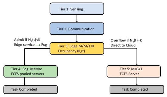
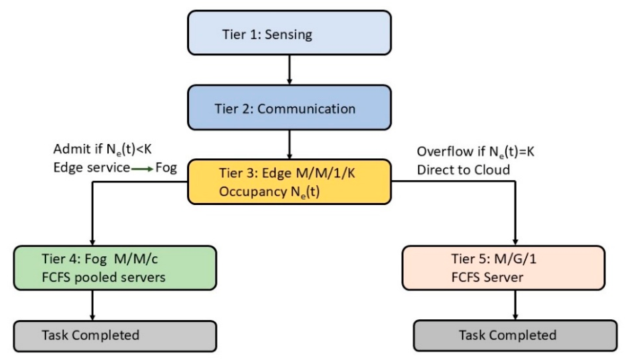
The QI-CPS architecture separates sensing, communication, edge, fog, and cloud functions and applies state-dependent routing at the finite-capacity edge tier. Sensor tasks first incur sensing and communication delays and then attempt admission to an edge M/M/1/K system. An arrival that observes fewer than K tasks is admitted, receives edge service, and subsequently enters the fog M/M/c tier. An arrival that observes K tasks is blocked from the edge and routed directly to the cloud M/G/1 tier. The overflow route therefore bypasses both edge service and fog processing. The analytical model and discrete-event simulation (DES) implement this topology consistently.

QI-CPS is formulated as a flow-coupled analytical decomposition rather than a classical open Jackson network [30]. Finite-capacity blocking produces state-dependent routing; the overflow stream is generally not Poisson, and the cloud has a general service-time distribution. Tier-level queueing models are therefore linked through explicit mean-flow equations, and the accuracy of the resulting end-to-end expression is evaluated using DES. The five functional tiers are: (i) sensing, with deterministic mean sensing delay D_s; (ii) communication, with route-dependent transmission delay; (iii) finite-buffer edge computing modeled as M/M/1/K; (iv) pooled fog computing modeled as FCFS M/M/c; and (v) cloud processing modeled as FCFS M/G/1. The fog tier follows the First-Come, First-Served (FCFS) discipline assumed by the Erlang-C formulation. Priority and QoS-differentiated scheduling are outside the scope of the analytical model. The resulting five-tier routing topology is illustrated in Figure 1.

Figure 1. Five-tier QI-CPS routing topology.

3.2. Edge and Fog Processing

The edge tier represents a field gateway executing time-sensitive inference and sensor fusion tasks. Its service rate is μ_e, and its capacity K includes the task in service. Finite capacity is essential because embedded agricultural gateways have bounded memory and compute resources. The fog tier aggregates the accepted output of one representative edge stream and supplies c statistically identical parallel servers, each with rate μ_f. Pooling provides additional capacity without changing the state-dependent decision made at the edge.

3.3. Cloud Processing

In the evaluated topology, the cloud receives only edge overflow traffic. Cloud service times are Gamma-distributed in the DES and are represented analytically by their first two moments in an M/G/1 model. This accommodates service-time variability associated with heterogeneous workloads such as model updates, batch analytics, and complex image processing jobs [31]. The baseline experiment includes no independent background cloud workload; if present, add such traffic directly to the cloud flow equation.

3.4. State-Dependent Cloud-Escalation Rule

Let N_e(t) be the number of tasks in the edge system immediately before an arrival at time t. The instantaneous routing decision R(t) is based on occupancy, not on a probability threshold:

$$R\left(t\right)=\left\{\begin{array}{ll}\mathrm{edge}\to \mathrm{fog},& N_e\left(t\right)<K,\\ \mathrm{cloud},& N_e\left(t\right)=K\end{array}\right.$$

(1)

where R(t) is the route assigned to the arrival at time t, N_e(t) is the instantaneous edge occupancy immediately before that arrival, and K is the total edge-system capacity, including any task in service.

Equation (1) is formulated in this study from the admission rule of a finite-capacity queue: an arrival is admitted when space is available; otherwise, it follows the cloud-overflow branch. The stationary blocking probability P_B = Pr{N_e = K} is the long-run fraction of Poisson arrivals expected to encounter a full edge system under the Poisson Arrivals See Time Averages (PASTA) property. It is therefore an outcome of the finite-buffer model, not an instantaneous control variable. The term blocking-aware escalation distinguishes this rule from fixed probabilistic offloading. Increasing K reduces escalation frequency but can increase the sojourn time of admitted tasks; reducing K shortens the local queue but can overload the cloud. Buffer selection must therefore consider latency and downstream stability jointly.

4. Mathematical Framework

4.1. Assumptions and Scope

A representative gateway receives a stationary Poisson task stream of rate λ_e. Edge and fog service times are independent and exponentially distributed with rates μ_e and μ_f, respectively. The fog contains c identical FCFS servers. Cloud service times are independent with mean ${\displaystyle \frac{1}{{\mu }_c}}$ and coefficient of variation c_v. The additive terms represent sensing and communication delays D_s, D_t, and D_ec, where D_t applies to the admitted edge-fog route and D_ec applies to direct edge-cloud escalation. Feedback, task duplication, retries, and independent cloud traffic are excluded from the baseline analysis. All reported steady-state analytical delays require the corresponding downstream stability conditions. Table 2 shows other symbols and definitions used in the analytical framework.

Table 2. Symbols and definitions used in the analytical framework.

Symbol	Definition	Unit or Range
λe, μe	Edge arrival and service rates	tasks/s
Ne(t), K	Instantaneous edge occupancy and total edge capacity	tasks; K = 1, …, 15
ρe, pn, PB	Offered edge utilization, state probability, and blocking probability	dimensionless
Le, We	Mean edge population and admitted-task edge sojourn time	tasks; s
λf, μf, c	Fog arrival rate, per-server service rate, and server count	tasks/s; c = 1, 2, 4, 8
af, ρf, Wf	Offered fog load, fog utilization, and mean fog sojourn time	dimensionless; s
λc, μc, ρc	Cloud arrival rate, mean service rate, and utilization	tasks/s; dimensionless
Sc, cv, Wc	Cloud service time, coefficient of variation, and mean cloud sojourn time	s; dimensionless; s
Ds, Dt, Dec	Mean sensing, admitted-route communication, and direct edge-cloud delays	s
TA, TB, E[T]	Admitted-route, blocked-route, and overall mean end-to-end latencies	s

4.2. Edge Tier: M/M/1/K

For the M/M/1/K edge model [14], the offered edge utilization is defined as ρ_e = ${\displaystyle \frac{{\lambda }_e}{{\mu }_e}}$, where, λ_e and μ_e denote the edge arrival rate and the edge service rate, respectively. The stationary occupancy probabilities are as follows

$$p_n=\left\{\begin{array}{ll}{\displaystyle \frac{(1-{\rho }_e){\rho }_e^n}{1-{\rho }_e^{K=1}}},& {\rho }_e\ne 1\\ {\displaystyle \frac{1}{K+1}},& {\rho }_e=1\end{array}\right.\hspace{1em}\mathrm{n}=0,1\dots ,\mathrm{K}$$

(2)

where p_n is the stationary probability that the edge contains n tasks, n is the occupancy state, and K is the total edge capacity.

The stationary blocking probability is as follows

$$P_B\left(K\right)=p_K={\displaystyle \frac{\left(1-{\rho }_e\right){\rho }_e^K}{1-{\rho }_e^{K+1}}}$$

(3)

where P_B(K) is the stationary blocking probability, and p_K is the probability that an arrival observes the full state K. Under Poisson arrivals, PASTA lets us interpret this full-state probability as the long-run blocked fraction [14].

The mean number of tasks at the edge and the admitted edge rate are as follows

$$L_e={\displaystyle \sum _{n=0}^K}n{p}_n.$$

(4)

λ_e,a = λ_e(1 − P_B)

(5)

where L_e is the mean number of tasks in the edge system and λ_e,a is the mean admitted arrival rate; all other symbols retain the definitions given above.

Because blocked arrivals do not enter the edge system, Little’s law applied to admitted tasks gives

$$W_e={\displaystyle \frac{L_e}{{\lambda }_e\left(1-P_B\right)}}$$

(6)

where W_e is the mean edge sojourn time of an admitted task. Equation (6) follows Little’s law applied to the admitted stream [14].

4.3. Branch Traffic Equations

Every admitted edge task proceeds to the fog, whereas every blocked arrival proceeds directly to the cloud. The mean branch rates are therefore

λ_f = λ_e(1 − P_B).

(7)

λ_c = λ_eP_B

(8)

where λ_f is the mean arrival rate to the fog, and λ_c is the mean overflow rate to the cloud. This study derives Equations (7) and (8) by applying flow conservation to the two mutually exclusive outcomes in Equation (1).

If an independent background cloud workload λ_c,b is introduced, the total cloud rate becomes λ_c,tot = λ_eP_B + λ_c,b. The present numerical study sets λ_c,b = 0 to isolate the consequences of edge overflow.

4.4. Fog Tier: FCFS M/M/c

For the FCFS M/M/c fog model [14,15], let a_f =${\displaystyle \frac{{\lambda }_f}{{\mu }_f}}$ and ρ_f = ${\displaystyle \frac{{\lambda }_f}{{\mathit{c\mu }}_f}}$, where a_f is the offered fog load, ρ_f is the fog utilization. For ρ_f < 1, the Erlang-C waiting probability and mean fog sojourn time are

$$C\left(c,a_f\right)={\displaystyle \frac{\frac{a_f^c}{c!\left(1-{\rho }_f\right)}}{{\displaystyle {\sum }_{n=0}^{c-1}}\frac{a_f^n}{n!}+\frac{a_f^c}{c!\left(1-{\rho }_f\right)}}}.$$

(9)

$$W_f={\displaystyle \frac{1}{{\mu }_f}}+{\displaystyle \frac{C\left(c,a_f\right)}{c{\mu }_f-{\lambda }_f}}$$

(10)

where c is the number of identical fog servers, μ_f is the service rate of each fog server, C (c, a_f) is the Erlang-C probability that an arrival waits, and W_f is the mean fog sojourn time.

Equations (9) and (10) are the standard FCFS M/M/c results [14,15].

4.5. Cloud Tier: M/G/1

The cloud utilization depends on K through the overflow probability, with ρ_c(K) = ${\displaystyle \frac{\mathsf{\lambda }\left(\mathrm{k}\right)}{{\mu }_c}}$ for ρ_c < 1, the Pollaczek-Khinchine M/G/1 result [14,15] gives

$$W_c\left(K\right)={\displaystyle \frac{1}{{\mu }_c}}+{\displaystyle \frac{{\lambda }_c\left(K\right)\mathrm{E} \left[S_c^2\right]}{2\left[1-{\rho }_c\left(K\right)\right]}}.$$

(11)

$$\mathrm{E} \left[S_c^2\right]={\displaystyle \frac{1+c_v^2}{{\mu }_c^2}}$$

(12)

where W_c(K) is the mean cloud sojourn time, ρ_c(K) =${\displaystyle \frac{\mathsf{\lambda }\left(\mathrm{k}\right)}{{\mu }_c}}$ is cloud utilization, μ_c is the reciprocal of the mean cloud service time, S_c is the cloud service time, E[S_c²] is its second moment, and c_v is its coefficient of variation.

Equations (11) and (12) follow the Pollaczek-Khinchine M/G/1 result and the second-moment identity E[S_c²] = Var (S_c) + E[S_c]² [14,15]. Thus, cloud delay is not a fixed escalation penalty. A smaller K increases P_B, which increases λ_c and can sharply increase W_c as ρ_c approaches one.

4.6. Route Conditioned End-to-End Latency

An admitted task follows sensing → communication → edge → fog, whereas a blocked task follows sensing → direct edge-cloud communication → cloud. The respective conditional mean route delays are as follows

T_A = D_s + D_t + W_e + W_f.

(13)

T_B = D_s + D_ec + W_c

(14)

where T_A is the conditional mean end-to-end latency of an admitted task, T_B is the conditional mean end-to-end latency of a blocked task, D_s is the mean sensing delay, D_t is the communication delay on the admitted edge-fog route, D_ec is the direct edge-cloud communication delay, and W_e, W_f, and W_c are the corresponding mean tier sojourn times.

Equations (13) and (14) are formulated from the two routes defined in Equation (1). The mean end-to-end latency across all arrivals is the route-probability-weighted quantity

E[T] = (1 − P_B)T_A + P_BT_B.

(15)

E[T] = D_s + (1 − P_B)(D_t + W_e + W_f) + P_B(D_ec + W_c)

(16)

where E[T] is the mean end-to-end latency over all arrivals.

Equations (15) and (16) are derived in this study by applying the law of total expectation to admitted and blocked routes, with probabilities 1 − P_B and P_B, respectively. This composition assigns edge and fog delays only to admitted tasks and cloud delay only to blocked tasks. It also captures the coupling P_B(K) → λ_c(K) → W_c(K). Because downstream arrival processes generated by finite-buffer routing need not be Poisson, this expression is treated as an engineering approximation based on mean-flow decomposition rather than an exact product-form solution.

4.7. Stability and Buffer-Selection Conditions

Although the finite-edge system is positive recurrent for any finite λ_e and μ_e, finite steady-state delays at the downstream queues require

λ_e[1 − P_B(K)] < cμ_f.

(17)

λ_eP_B(K) < μ_c

(18)

where the left side of Equation (17) is the fog arrival rate, and cμ_f is the aggregate fog service capacity, while the left side of Equation (18) is the cloud arrival rate, and μ_c is the cloud service capacity.

These inequalities apply the standard condition that the arrival rate must remain below service capacity for a stable downstream queue [14,15]. A feasible buffer capacity must satisfy both inequalities. The design problem is therefore

$$K^{*}=\underset{\begin{array}{c}K\in \{1,\dots ,15\}\\ {\lambda }_e\left[1-P_B\left(K\right)\right]<c{\mu }_f\\ {\lambda }_e{P}_B\left(K\right)<{\mu }_c\end{array}}{\arg \min }\hspace{0.25em}\mathrm{E}\left[T\left(K\right)\right]$$

(19)

where K* is the latency-minimizing feasible edge capacity among the tested integer values K = 1, …, 15. Equation (19) defines the design criterion proposed in this study: minimizing route-conditioned mean latency subject to the downstream stability conditions established in (17) and (18).

4.8. Performance Measures

The study reports P_B, accepted and overflow rates, fog and cloud utilizations, tier sojourn times, route-conditioned mean end-to-end latency, 95% confidence intervals for DES estimates, the analytical DES percentage difference, the feasible stability region, and the analytical and simulated minimizing capacities.

5. Simulation Methodology

End-to-End Discrete-Event Simulation

A custom event-driven DES reproduces the complete routing topology. Poisson arrivals attempt edge admission. Accepted tasks receive exponential edge service and, at edge completion, join the common FCFS queue feeding c exponential fog servers. Blocked tasks bypass the edge and fog and immediately join a single FCFS cloud server with Gamma-distributed service time. The Gamma shape and scale are selected to produce a mean of ${\displaystyle \frac{1}{{\mathsf{\mu }}_c}}$ and a coefficient of variation c_v = 1.3. Constant sensing and route-appropriate communication delays are added to each task’s completion time. The experiment covers K = 1, …, 15, ρ_e = 0.5, 0.6, 0.7, 0.8, 0.9, and c = 1, 2, 4, 8, for 300 configurations. Each configuration uses five independent replications. The first 3000 generated arrivals are treated as warm-up observations, followed by 30,000 measured arrivals per replication. Reproducible deterministic seeds are assigned by configuration and replication. Means are computed across replications, and the 95% confidence intervals use 1.96 times the replication standard error. Configurations violating either downstream stability condition are labeled unstable and excluded from steady-state optimization rather than summarized using finite-run transient delays. The final analytical and DES experiment settings are summarized in Table 3.

Table 3. Final analytical and DES experiment settings.

Parameter	Value	Role
Edge arrival rate	λe = ρe × 60 tasks/s	Offered workload
Edge service	μe = 60 tasks/s; exponential	M/M/1/K
Edge capacity	K = 1, …, 15 (includes service)	Design variable
Fog service	μf = 25 tasks/s/server; exponential	M/M/c
Fog servers	c = 1, 2, 4, 8	Provisioning factor
Cloud service	μc = 15 tasks/s; Gamma, cv = 1.3	M/G/1
Fixed delays	Ds = 20 ms; Dt = Dec = 4.5 ms	Route latency
Replications	5 per configuration	Independent estimates
Warm-up/measured	3000/30,000 arrivals per replication	Transient removal/run length
Confidence interval	95% replication-based CI	DES uncertainty

6. Results

6.1. Blocking and Coupled Downstream Load

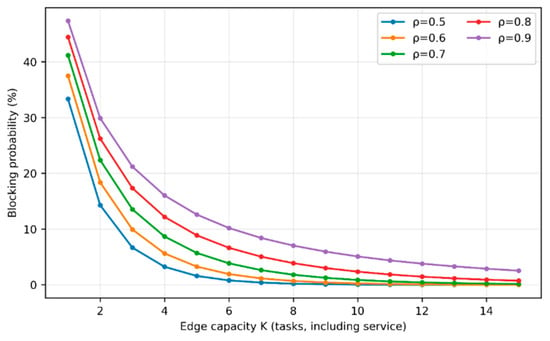
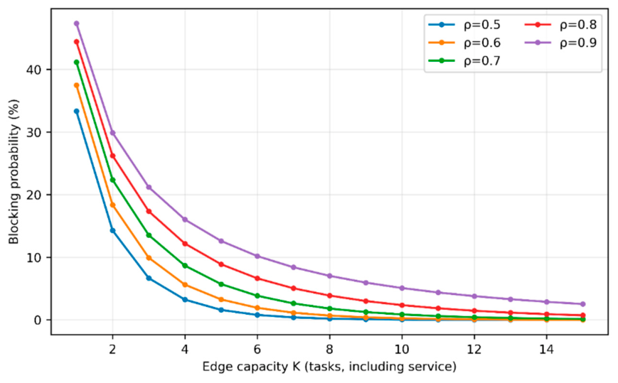
Figure 2 shows that P_B decreases monotonically with K but increases with offered edge utilization. This local improvement does not imply monotonic system improvement: reducing P_B transfers traffic from the cloud branch to the fog branch and simultaneously changes the conditional edge delay. Consequently, the same capacity adjustment can relieve one downstream tier while loading the other.

Figure 2. Edge blocking probability versus capacity K for the tested offered edge utilizations.

6.2. Analytical and DES Capacity Sensitivity

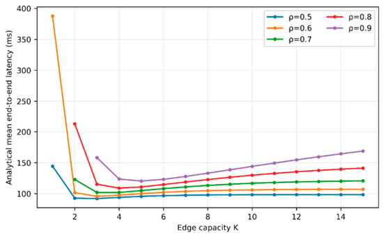
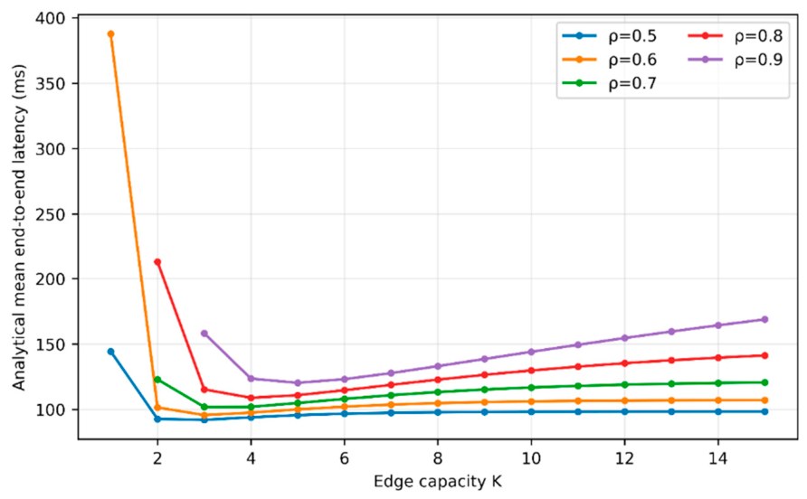
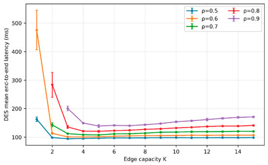
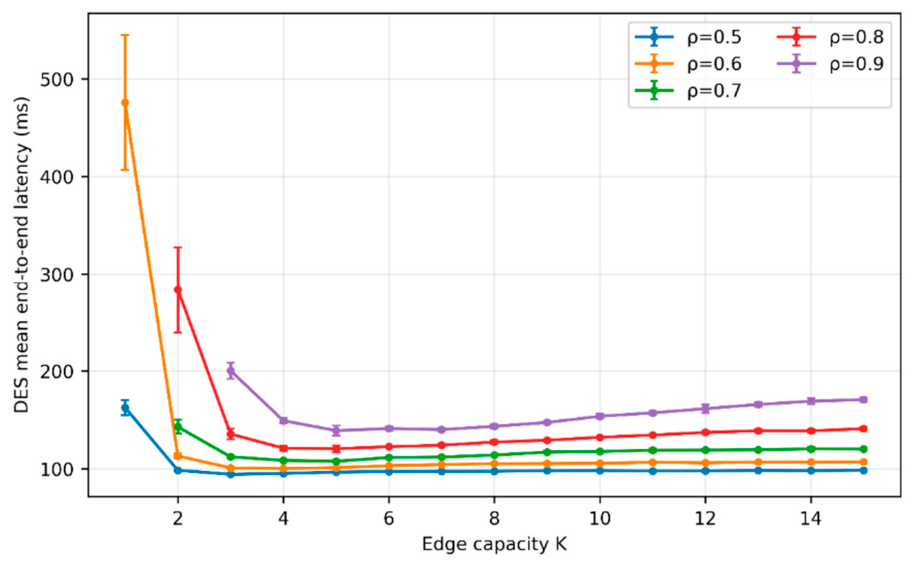
Figure 3 and Figure 4 show the analytical and DES latency surfaces, respectively, for c = 4. Both exhibit a low-latency interior region among stable capacities. Small K can overload the cloud through overflow; increasing K keeps more tasks at the edge and shifts additional completed traffic to the fog.

Figure 3. Analytical route-conditioned mean end-to-end latency versus edge capacity for c = 4.

Figure 4. End-to-end DES mean latency and 95% confidence intervals versus edge capacity for c = 4.

The analytical surface is a mean-flow approximation, whereas the DES surface represents the implemented state-dependent event process. Differences between neighboring minima should therefore be interpreted alongside replication uncertainty.

6.3. Analytical and DES Capacity Sensitivity at the Baseline Operating Point

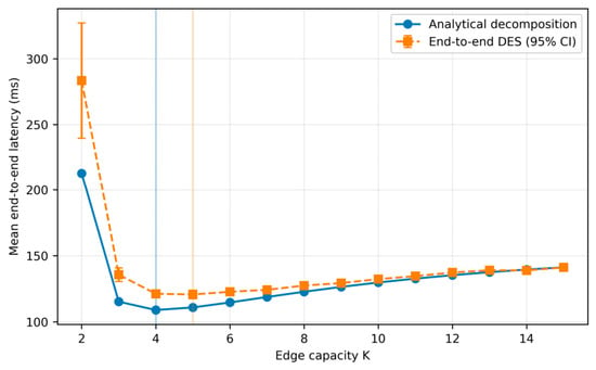
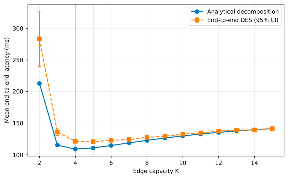
At ρ_e = 0.8 and c = 4, Figure 5 and Table 4 compare analytical and DES mean latency. K = 1 is cloud-unstable (P_B = 0.444, λ_c ≈ 21.33 tasks/s, ρ_c ≈ 1.42). The analytical point estimate is lowest at K = 4 (108.9 ms). The DES point estimate is lowest at K = 5 (120.7 ± 3.2 ms), while K = 4 gives 121.2 ± 2.7 ms. Their 0.5 ms difference is small relative to the reported 95% confidence interval half-widths. These separate intervals do not constitute a paired comparison, and their overlap alone is not a formal significance test. The manuscript does not report the five replication-level paired differences, so the data do not establish a unique DES-optimal capacity. K = 4–5 is a near-optimal candidate range for this operating point; a direct replicated comparison would be needed to distinguish the two statistically.

Figure 5. Analytical and DES capacity sensitivity at ρ_e = 0.8 and c = 4.

Table 4. Capacity sensitivity at ρ_e = 0.8 and c = 4.

K	PB (%)	Cloud ρc	Analytical E[T] (ms)	DES E[T] ± 95% CI (ms)
1	44.4	1.422	Unstable	Unstable
2	26.2	0.839	212.8	283.5 ± 43.8
3	17.3	0.555	115.3	135.7 ± 5.2
4	12.2	0.390	108.9	121.2 ± 2.7
5	8.9	0.284	110.9	120.7 ± 3.2
6	6.6	0.212	114.7	122.7 ± 0.6
7	5.0	0.161	118.8	124.2 ± 1.5
8	3.9	0.124	122.8	127.4 ± 1.8
9	3.0	0.096	126.4	129.3 ± 1.1
10	2.3	0.075	129.8	132.3 ± 0.8
11	1.8	0.059	132.7	134.6 ± 0.8
12	1.5	0.047	135.3	137.3 ± 1.6
13	1.2	0.037	137.6	139.0 ± 1.3
14	0.9	0.029	139.6	138.9 ± 1.6
15	0.7	0.023	141.3	141.1 ± 1.7

The analytical and simulated point minima fall at neighboring capacities. The decomposition treats λ_c = λ_eP_B as an effective mean input rate in an M/G/1 formula; actual overflow epochs in DES retain dependence on the full-buffer state. Fog input likewise reflects edge admission and departures. The two approaches thus identify a similar candidate region, while their numerical differences illustrate approximation error. The available summary statistics do not support a precise ordering of K = 4 and K = 5.

The difference between K* analytical and K* DES is methodologically meaningful. The decomposition uses λ_c = λ_eP_B as an effective mean rate and applies the M/G/1 formula as though the overflow input were Poisson. In the DES, overflow epochs are generated by the actual full-buffer state and retain temporal dependence. Departures into fog are likewise shaped by edge service and admission. The analytical formulation therefore identifies a useful design neighborhood, while the DES resolves the integrated operational optimum. The result does not support an exact Jackson product-form interpretation.

6.4. Workload- and Fog-Dependent Optimal Capacity

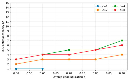
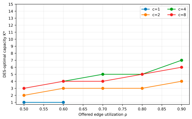
Figure 6 plots the capacity with the smallest observed DES mean in each tested configuration. These are point-estimate minimizers, not statistically established unique optima. As offered utilization increases, larger buffers often reduce cloud overflow; the fog capacity determines whether this additional admitted load remains stable. Four and eight fog servers often yield neighboring candidate capacities, and several higher-load cases with c = 1 have no feasible steady-state capacity. The plotted capacities should guide shortlisting; close alternatives require direct replicated comparisons.

Figure 6. Capacity with the smallest observed DES mean for each tested workload and fog-server configuration.

6.5. Minimum Achievable Latency and Fog Provisioning

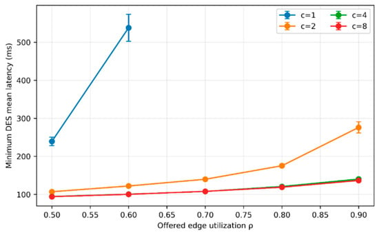
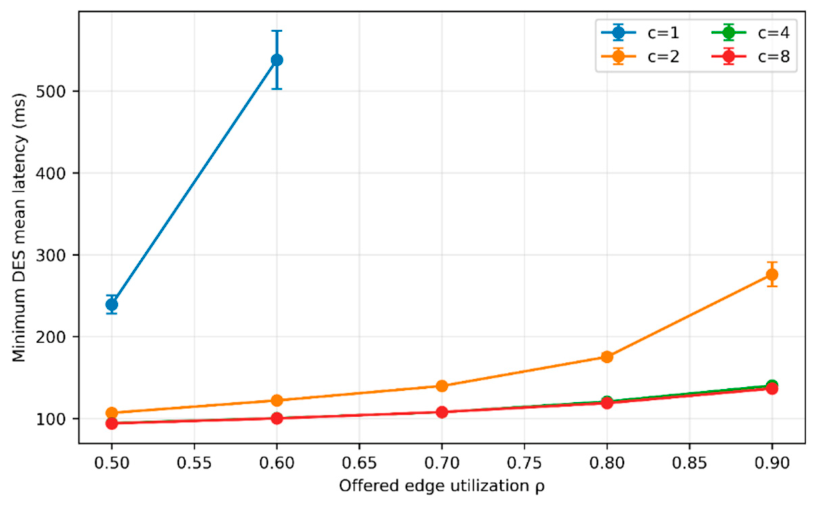
For each workload and fog configuration, Figure 7 shows the minimum simulated latency attainable for K = 1, …, 15. Moving from one to multiple fog servers expands the feasible region and reduces latency. Four fog servers provide a robust operating region across the tested loads; eight servers offer a smaller incremental benefit because the edge and cloud branches then account for a larger share of system latency. This result supports balanced provisioning rather than unbounded fog scaling.

Figure 7. Minimum stable DES mean end-to-end latency versus offered edge utilization for c = 1, 2, 4, and 8, with 95% confidence intervals.

6.6. Stability-Constrained Design Region

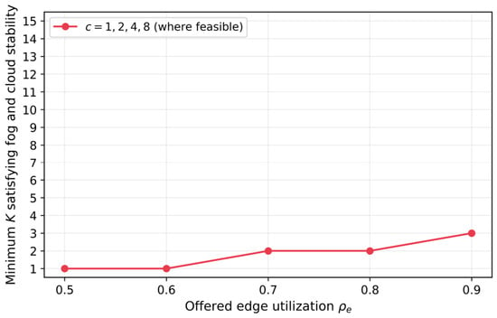
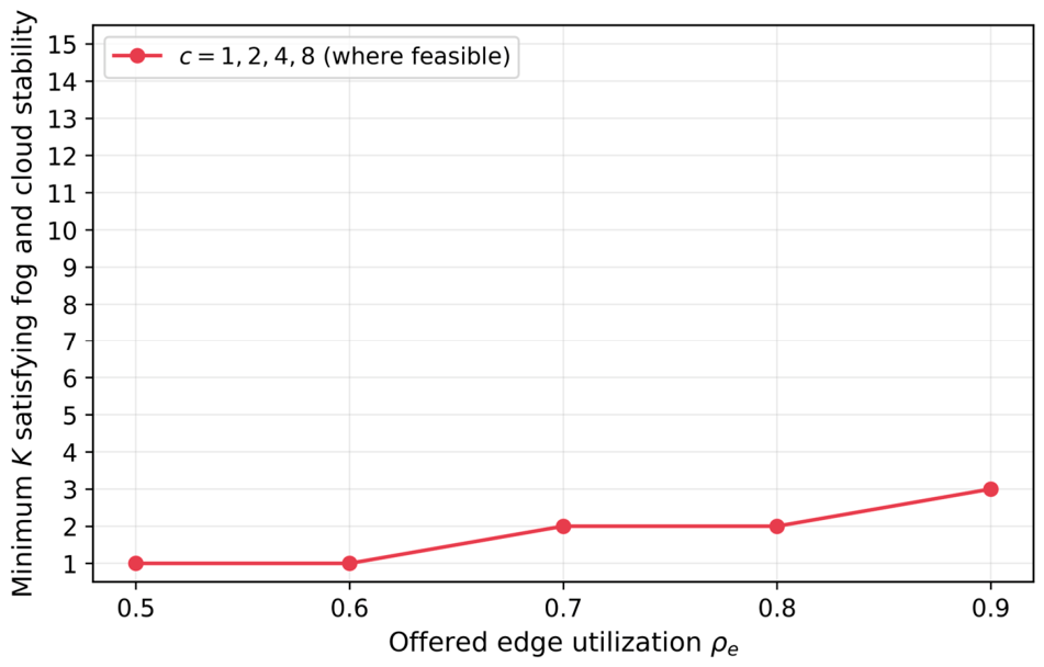
Figure 8 reports the smallest K satisfying both downstream stability conditions. The cloud condition places a lower bound on K because smaller buffers create more overflow. The fog condition can place an upper bound on K when c is small because admitted traffic increases as blocking falls. These coupled constraints explain why a locally attractive edge setting can be infeasible for the system as a whole. Table 5 summarizes the analytical and DES point-estimate minimizing capacities across workloads and fog configurations.

Figure 8. Minimum edge capacity satisfying both λ_e(1 − P_B) < cμ_f and λ_eP_B < μ_c.

Table 5. Analytical and DES point-estimate minimizing capacities across workloads and fog configurations.

c	ρe	Analytical K*	DES K*	Minimum DES E[T] ± 95% CI (ms)
1	0.5	1	1	239.4 ± 11.3
1	0.6	1	1	538.0 ± 35.3
1	0.7	—	—	Unstable
1	0.8	—	—	Unstable
1	0.9	—	—	Unstable
2	0.5	2	2	107.0 ± 1.3
2	0.6	2	3	122.1 ± 2.1
2	0.7	3	3	139.8 ± 2.6
2	0.8	3	3	175.4 ± 4.1
2	0.9	3	4	276.0 ± 14.8
4	0.5	3	3	94.5 ± 0.2
4	0.6	3	4	100.5 ± 0.4
4	0.7	3	5	107.8 ± 1.2
4	0.8	4	5	120.7 ± 3.2
4	0.9	5	7	140.2 ± 1.9
8	0.5	3	3	94.1 ± 0.4
8	0.6	3	4	100.2 ± 1.0
8	0.7	4	4	108.0 ± 1.0
8	0.8	4	5	118.9 ± 1.2
8	0.9	5	6	136.7 ± 2.1

7. Discussion

7.1. Analytical Approximation Versus Integrated DES

The tier formulas expose causal design relationships and can be evaluated rapidly. Agreement with isolated canonical queues, however, is insufficient to establish the performance of the complete architecture. The end-to-end DES provides a system-level evaluation because it implements the same admission state, branch routing, service distributions, and resource contention without replacing overflow traffic with an independent Poisson stream. The difference observed near the optimum quantifies the practical effect of mean-flow decomposition and defines the level of analytical accuracy available for capacity screening.

For well-provisioned fog cases, the analytical curves can guide screening. Final capacity selection should compare nearby alternatives using replication-level paired differences or additional independent replications, especially when estimated differences are small. Measured arrival burstiness, network delays, and service-time distributions can also shift the candidate region.

7.2. Implications for Agricultural CPS Design

Three implications follow. First, edge blocking is a routing outcome with system-wide consequences, not merely a local loss metric. Second, more edge buffering is not always better: larger K lowers cloud overflow but increases local retention and sends more completed traffic toward fog. Third, fog and cloud must be sized together. A deployment that tunes K using edge latency alone can move congestion downstream and may cross a stability boundary.

For resource-constrained agricultural deployments, the model provides a practical sequence: estimate λ_e and μ_e from gateway telemetry; evaluate P_B(K); reject capacities that violate either downstream stability inequality; use the analytical decomposition to shortlist candidate capacities; and confirm the shortlist with DES driven by measured traffic and service distributions. This sequence is more robust than applying a fixed cloud-delay penalty or selecting a single universal K.

7.3. Limitations

The baseline uses stationary Poisson input, exponential edge and fog service, a single representative gateway flow, constant mean communication delays, and no independent cloud workload. The warm-up is specified by arrival count rather than by a formal transient-deletion diagnostic. Replication-based confidence intervals quantify stochastic error but not model-form uncertainty. The analytical branch models use effective mean arrival rates even though overflow and departure streams can be non-Poisson. Finally, the parameter values are design-study settings rather than measurements from a deployed farm, so the reported optima should not be transferred unchanged to another workload.

7.4. Future Validation

Future work should replace the baseline source with bursty Markov-modulated or empirical agricultural traces; estimate service distributions from edge accelerators and cloud jobs; include route-specific stochastic communication delay, failures, retries, and background cloud traffic; and extend the topology to multiple gateways sharing fog capacity. Priority scheduling and learning-based admission control should be evaluated in DES with queueing models appropriate to those disciplines. Releasing the simulation code, configuration data, and seeds will also support independent reproduction and comparison.

8. Conclusions

This paper presented QI-CPS, a five-tier queueing-theoretic architecture for agricultural automation with finite-buffer edge processing and state-dependent cloud escalation. We coupled canonical edge, fog, and cloud queues through explicit branch-flow equations and a route-conditioned analytical decomposition, then evaluated the results with an integrated DES. Buffer selection must satisfy both fog and cloud stability constraints. At ρ_e = 0.8 and c = 4, K = 1 overloads the cloud; the analytical point estimate is lowest at K = 4, while DES produces similar means at K = 4 and K = 5 (121.2 ± 2.7 and 120.7 ± 3.2 ms, respectively). The reported summary intervals cannot establish a unique DES optimum, so K = 4–5 is the near-optimal capacity range. Across workloads and fog capacities, the point-estimate minimizing capacity changes, and some configurations lack a feasible steady state. The framework supports stability screening and simulation-based comparison of neighboring designs, while future work will focus on validating its performance using field traces.

References

- FAO. The Future of Food and Agriculture: Trends and Challenges; Food and Agriculture Organization of the United Nations: Rome, Italy, 2017. [Google Scholar]
- Wolfert, S.; Ge, L.; Verdouw, C.; Bogaardt, M.-J. Big Data in Smart Farming—A review. Agric. Syst. 2017, 153, 69–80. [Google Scholar] [CrossRef] [Scilit]
- Verdouw, C.N.; Wolfert, J.; Beulens, A.J.M.; Rialland, A. Virtualization of food supply chains with the internet of things. J. Food Eng. 2016, 176, 128–136. [Google Scholar] [CrossRef] [Scilit]
- Lee, E.A. Cyber Physical Systems: Design Challenges. In Proceedings of the 2008 11th IEEE International Symposium on Object and Component-Oriented Real-Time Distributed Computing (ISORC), Orlando, FL, USA, 5–7 May 2008; pp. 363–369. [Google Scholar] [CrossRef] [Scilit]
- Gutierrez, J.; Villa-Medina, J.F.; Nieto-Garibay, A.; Porta-Gandara, M.A. Automated Irrigation System Using a Wireless Sensor Network and GPRS Module. IEEE Trans. Instrum. Meas. 2014, 63, 166–176. [Google Scholar] [CrossRef] [Scilit]
- Ferentinos, K.P. Deep learning models for plant disease detection and diagnosis. Comput. Electron. Agric. 2018, 145, 311–318. [Google Scholar] [CrossRef] [Scilit]
- Kamilaris, A.; Prenafeta-Boldú, F.X. Deep learning in agriculture: A survey. Comput. Electron. Agric. 2018, 147, 70–90. [Google Scholar] [CrossRef] [Scilit]
- Bac, C.W.; Van Henten, E.J.; Hemming, J.; Edan, Y. Harvesting Robots for High-value Crops: State-of-the-art Review and Challenges Ahead. J. Field Robot. 2014, 31, 888–911. [Google Scholar] [CrossRef] [Scilit]
- Zhang, C.; Kovacs, J.M. The application of small unmanned aerial systems for precision agriculture: A review. Precis. Agric. 2012, 13, 693–712. [Google Scholar] [CrossRef] [Scilit]
- Boursianis, A.D.; Papadopoulou, M.S.; Diamantoulakis, P.; Liopa-Tsakalidi, A.; Barouchas, P.; Salahas, G.; Karagiannidis, G.; Wan, S.; Goudos, S.K. Internet of Things (IoT) and Agricultural Unmanned Aerial Vehicles (UAVs) in smart farming: A comprehensive review. Internet Things 2022, 18, 100187. [Google Scholar] [CrossRef] [Scilit]
- Deng, R.; Lu, R.; Lai, C.; Luan, T.H.; Liang, H. Optimal Workload Allocation in Fog-Cloud Computing Towards Balanced Delay and Power Consumption. IEEE Internet Things J. 2016, 3, 1171–1181. [Google Scholar] [CrossRef] [Scilit]
- Fan, Q.; Ansari, N. Application Aware Workload Allocation for Edge Computing-Based IoT. IEEE Internet Things J. 2018, 5, 2146–2153. [Google Scholar] [CrossRef] [Scilit]
- Erlang, A.K. Solution of some problems in the theory of probabilities of significance in automatic telephone exchanges. Post. Off. Electr. Eng. J. 1917, 10, 189–197. [Google Scholar]
- Kleinrock, L. Queueing Systems; Wiley: New York, NY, USA, 1975; Volume 1: Theory. [Google Scholar]
- Kleinrock, L. Queueing Systems; Wiley: New York, NY, USA, 1976; Volume 2: Computer Applications. [Google Scholar]
- Gross, D.; Shortle, J.F.; Thompson, J.M.; Harris, C.M. Fundamentals of Queueing Theory, 4th ed.; Wiley-Interscience: Hoboken, NJ, USA, 2008. [Google Scholar] [CrossRef] [Scilit]
- Ghosh, R.; Longo, F.; Naik, V.K.; Trivedi, K.S. Modeling and performance analysis of large scale IaaS Clouds. Future Gener. Comput. Syst. 2013, 29, 1216–1234. [Google Scholar] [CrossRef] [Scilit]
- Mao, Y.; You, C.; Zhang, J.; Huang, K.; Letaief, K.B. A Survey on Mobile Edge Computing: The Communication Perspective. IEEE Commun. Surv. Tutor. 2017, 19, 2322–2358. [Google Scholar] [CrossRef] [Scilit]
- Mach, P.; Becvar, Z. Mobile Edge Computing: A Survey on Architecture and Computation Offloading. IEEE Commun. Surv. Tutor. 2017, 19, 1628–1656. [Google Scholar] [CrossRef] [Scilit]
- Shi, W.; Cao, J.; Zhang, Q.; Li, Y.; Xu, L. Edge Computing: Vision and Challenges. IEEE Internet Things J. 2016, 3, 637–646. [Google Scholar] [CrossRef] [Scilit]
- Bonomi, F.; Milito, R.; Zhu, J.; Addepalli, S. Fog computing and its role in the internet of things. In Proceedings of the First Edition of the MCC Workshop on Mobile Cloud Computing, Helsinki Finland, 17 August 2012; pp. 13–16. [Google Scholar] [CrossRef] [Scilit]
- Botta, A.; De Donato, W.; Persico, V.; Pescapé, A. Integration of Cloud computing and Internet of Things: A survey. Future Gener. Comput. Syst. 2016, 56, 684–700. [Google Scholar] [CrossRef] [Scilit]
- Chen, X.; Jiao, L.; Li, W.; Fu, X. Efficient Multi-User Computation Offloading for Mobile-Edge Cloud Computing. IEEE/ACM Trans. Netw. 2015, 24, 2795–2808. [Google Scholar] [CrossRef] [Scilit]
- Tzounis, A.; Katsoulas, N.; Bartzanas, T.; Kittas, C. Internet of Things in agriculture, recent advances and future challenges. Biosyst. Eng. 2017, 164, 31–48. [Google Scholar] [CrossRef] [Scilit]
- Muangprathub, J.; Boonnam, N.; Kajornkasirat, S.; Lekbangpong, N.; Wanichsombat, A.; Nillaor, P. IoT and agriculture data analysis for smart farm. Comput. Electron. Agric. 2019, 156, 467–474. [Google Scholar] [CrossRef] [Scilit]
- Elijah, O.; Rahman, T.A.; Orikumhi, I.; Leow, C.Y.; Hindia, M.H.D.N. An Overview of Internet of Things (IoT) and Data Analytics in Agriculture: Benefits and Challenges. IEEE Internet Things J. 2018, 5, 3758–3773. [Google Scholar] [CrossRef] [Scilit]
- Gubbi, J.; Buyya, R.; Marusic, S.; Palaniswami, M. Internet of Things (IoT): A vision, architectural elements, and future directions. Future Gener. Comput. Syst. 2013, 29, 1645–1660. [Google Scholar] [CrossRef] [Scilit]
- Ray, P.P. Internet of things for smart agriculture: Technologies, practices and future direction. AIS 2017, 9, 395–420. [Google Scholar] [CrossRef] [Scilit]
- Bechar, A.; Vigneault, C. Agricultural robots for field operations: Concepts and components. Biosyst. Eng. 2016, 149, 94–111. [Google Scholar] [CrossRef] [Scilit]
- Jackson, J.R. Networks of Waiting Lines. Oper. Res. 1957, 5, 518–521. [Google Scholar] [CrossRef] [Scilit]
- Rana, S.; Hensel, O.; Nasirahmadi, A. Generative semantic reconstruction for annotation-ready vegetation priors in spectrally heterogeneous imagery. MethodsX 2026, 16, 103967. [Google Scholar] [CrossRef] [Scilit]
Disclaimer/Publisher’s Note: The statements, opinions and data contained in all publications are solely those of the individual author(s) and contributor(s) and not of MDPI and/or the editor(s). MDPI and/or the editor(s) disclaim responsibility for any injury to people or property resulting from any ideas, methods, instructions or products referred to in the content. |
© 2026 by the authors. Licensee MDPI, Basel, Switzerland. This article is an open access article distributed under the terms and conditions of the Creative Commons Attribution (CC BY) license.