R-Matrix Theory for Transport in Interacting Semiconductor Quantum Devices: Local Density Approximation and Weak Formulation

Abstract

In a series of publications, a scattering theory of quantum transport in mesoscopic semiconductor devices was developed in the R-matrix formalism. Recently, the R-matrix theory was cast in the weak formulation for non-interacting systems. In this paper we extend this theory to take into account the Coulomb interaction within the local density approximation of the density functional theory by Hohenberg, Kohn, and Sham. As a major advantage, the weak formulation formalism allows us to introduce a wide class of approximations by choosing appropriate basis functions. Here we implement the spectral element method for numerical purposes, which is a version of the finite element method that uses high-degree piecewise polynomials (Lagrange elements) as basis functions. Important for the density functional theory we derive an expansion of the carrier density in Wigner–Eisenbud functions in which the energy integration becomes space-independent. Finally we cast the Poisson equation in weak formulation as well to obtain a self-consistency loop for iteratively solving the local density approximation.

1. Introduction

A scattering theory of quantum transport in mesoscopic semiconductor devices was previously developed in the R-matrix formalism [1,2,3,4,5]. Examples for the application of this approach include conventional MOSFETs [3], nanowire transistors [6], spin-FETs [7], quantum logic gates [8], SOI-transistors [9], and the two-channel transistor was proposed as a new device architecture based on SOI-technology [10].

For non-interacting systems, the application of the weak formulation method to the Schrödinger scattering problem was demonstrated in the quantum transmitting boundary method by Lent and Kirkner [11,12,13,14,15]. The weak formulation is an important tool for systematizing approximations and for numerically calculating the transmission coefficients of the scattering states, which are the crucial quantities required to determine the device current. In the weak formulation, the wave function is assumed to be a linear combination of properly chosen basis functions (corresponding to “atomic orbitals” in the LCAO approximation).

In Ref. [16] the R-matrix method was cast in weak formulation. As a major advantage, the R-matrix method enables the systematic introduction of current conserving approximations to the Schrödinger scattering problem in the weak formulation. In this paper, we extend our theory to take into account the Coulomb interaction between the charge carriers. Generally, the total potential seen by the charge carriers is strongly influenced by the Coulomb interaction in semiconductor nano-devices. Here we apply the local density approximation (LDA) of the density functional theory by Hohenberg, Kohn, and Sham [17,18]. The resulting Kohn–Sham equation replaces the Schrödinger equation, retaining the same structure so that we can directly apply our R-matrix theory.

The density functional formalism has been applied to open, current-carrying systems in Refs. [19,20] using the non-equilibrium Green’s function (NEGF) formalism. In contrast to the NEGF in which the self-energies for the Green’s functions are formulated on a grid from the start, the R-matrix formalism starts from an exact reformulation of the Schrödinger scattering problem in the continuum (see Appendix A). As a major advantage, by introducing the weak formulation formalism it is possible to generate a wider class of approximations by freely choosing appropriate atomic orbitals that are not necessarily bound to a grid. One example is cosine functions as basis functions, for which the fundamental completeness and expansion theorems are well-known in the Fourier theory, allowing for a generalization in the Sturm–Liouville theory [21]. These theorems are necessary to reformulate the Schrödinger scattering problem exactly. Here we focus on the implementation of the spectral element method for numerical purposes, which is a version of the finite element method that uses high-degree piecewise polynomials (Lagrange elements) as basis functions [22,23].

It is evident that in the density functional formalism, the central issue is the construction of the charge density. In principle, in the open system it has to be calculated for each space point and for each point of the energy-continuum of the scattering states. To simplify this numerical problem we derive in Section 2 an expansion of the charge density in the Wigner–Eisenbud functions. The Wigner–Eisenbud functions appear naturally in the R-matrix formalism and turn out to be the natural basis for the expansion of the charge density because of the Neumann boundary conditions they fulfill. In the expansion of the particle density in Wigner–Eisenbud functions, the necessary energy integration becomes independent of the space argument, which is a considerable numerical advantage. Finally, in Section 4 we formulate Poisson’s equation in weak formulation. This yields a self-consistency loop, which is typical of this type of problem.

2. Density Functional Theory for Open Systems in the 1d-Slab Model

We start from the Kohn–Sham equation

$$\left(-{\displaystyle \frac{{\hslash }^2}{2m}}{\nabla }^2+V\left(\mathbf{r}\right)-E_{\lambda }\right){\varphi }_{\lambda }\left(\mathbf{r}\right)=0,$$

(1)

where ${\varphi }_{\lambda }$ are the Kohn–Sham orbitals and the $E_{\lambda }$ are the corresponding orbital energies [17,18]. The effective Kohn–Sham potential (“total potential”) V is given by

$$V\left(\overrightarrow{r}\right)=v_{ext}\left(\overrightarrow{r}\right)+v_H\left(\overrightarrow{r}\right)+v_{xc}\left(\overrightarrow{r}\right).$$

(2)

The three components of the total potential result from the minimization of the corresponding factors of the ground-state energy functional with respect carrier density n,

$$V\left(\overrightarrow{r}\right)={\displaystyle \frac{\delta E\left[n\right]}{\delta n\left(\overrightarrow{r}\right)}}$$

(3)

with

$$E\left[n\right]=E_{ext}\left[n\right]+E_H\left[n\right]+E_{xc}\left[n\right],$$

(4)

as described in detail below.

-

External potential $v_{ext}$: In the context of semiconductor nanostructures, the external potential comprises the electrostatic potential of background charges of charge density ${\rho }_b\left(\overrightarrow{r}\right)$ (ionized impurities) and the band-offset potential $v_{off}\left(\overrightarrow{r}\right)$, which results in the mesoscopic effective mass approximation. We write for the negative electrons

$$E_{ext}\left[n\right]=\int d^{3}rn\left(\overrightarrow{r}\right)\left[v_{off}\left(\overrightarrow{r}\right)-{\displaystyle \frac{e}{4\pi {\kappa }_0\kappa }}\int d^3{r}^{\prime }{\displaystyle \frac{{\rho }_b\left({\overrightarrow{r}}^{\prime }\right)}{|\overrightarrow{r}-{\overrightarrow{r}}^{\prime }|}}\right]$$

(5)

so that

$$v_{ext}\left(\overrightarrow{r}\right)={\displaystyle \frac{\delta E_{ext}\left[n\right]}{\delta n\left(\overrightarrow{r}\right)}}=v_{off}\left(\overrightarrow{r}\right)-{\displaystyle \frac{e}{4\pi {\kappa }_0\kappa }}\int d^3{r}^{\prime }{\displaystyle \frac{{\rho }_b\left({\overrightarrow{r}}^{\prime }\right)}{|\overrightarrow{r}-{\overrightarrow{r}}^{\prime }|}}.$$

(6)

For simplicity we neglect the space-dependence of the dielectric constant $\kappa$, which can be taken into account in a straightforward way.

-

Hartree potential $v_H$: As usual, the Hartree potential results from the functional of the classical Coulomb energy

$$E_H\left[n\right]={\displaystyle \frac{e^2}{8\pi {\kappa }_0\kappa }}\int d^{3}r\int d^3{r}^{\prime }{\displaystyle \frac{n\left(\overrightarrow{r}\right)n\left({\overrightarrow{r}}^{\prime }\right)}{|\overrightarrow{r}-{\overrightarrow{r}}^{\prime }|}}.$$

(7)

It is given by

$$v_H\left(\overrightarrow{r}\right)={\displaystyle \frac{\delta E_H\left[n\right]}{\delta n\left(\overrightarrow{r}\right)}}={\displaystyle \frac{e^2}{4\pi {\kappa }_0\kappa }}\int d^3{r}^{\prime }{\displaystyle \frac{n\left({\overrightarrow{r}}^{\prime }\right)}{|\overrightarrow{r}-{\overrightarrow{r}}^{\prime }|}}.$$

(8)

Here, the ground-state carrier density n at $T=0$ is constructed from the occupied Kohn–Sham orbitals,

$$n\left(\overrightarrow{r}\right)=\sum _{\lambda }\mathrm{\Theta }(E_F-E_{\lambda }){\left|{\varphi }_{\lambda }\left(\overrightarrow{r}\right)\right|}^2,$$

(9)

where $E_F$ is the Fermi energy.

-

Exchange-correlation potential $v_{xc}$: In the LDA the exchange-correlation functional is given by

$$E_{xc}^{\mathrm{LDA}}\left[n\right]=\int d^{3}rf\left(n\left(\overrightarrow{r}\right)\right)$$

(10)

with a suitably chosen function f representing the assumed only-particle density-dependent exchange-correlation energy density. Because f depends only on the local density, the Euler–Lagrange equation yields

$$v_{xc}^{\mathrm{LDA}}\left(\overrightarrow{r}\right)={\displaystyle \frac{\delta E_{\mathrm{xc}}^{\mathrm{LDA}}\left[n\right]}{\delta n\left(\overrightarrow{r}\right)}}={\displaystyle \frac{\partial f}{\partial n}}.$$

(11)

In the following, it is more convenient to rearrange the three terms in (2) slightly writing

$$v_{ext}\left(\overrightarrow{r}\right)=v_{off}\left(\overrightarrow{r}\right)$$

(12)

and, for the negative electron,

$$v_H\left(\overrightarrow{r}\right)=-{\displaystyle \frac{e}{4\pi {\kappa }_0\kappa }}\int d^3{r}^{\prime }{\displaystyle \frac{\rho \left({\overrightarrow{r}}^{\prime }\right)}{|\overrightarrow{r}-{\overrightarrow{r}}^{\prime }|}},$$

(13)

where $\rho \left(\overrightarrow{r}\right)=-en\left(\overrightarrow{r}\right)+{\rho }_b\left(\overrightarrow{r}\right)$ is the total charge density. The Hartree potential fulfills the Poisson equation

$$\Delta v_H\left(\overrightarrow{r}\right)={\displaystyle \frac{e}{{\kappa }_0\kappa }}\rho \left(\overrightarrow{r}\right).$$

(14)

The exchange-correlation potential (11) remains unchanged.

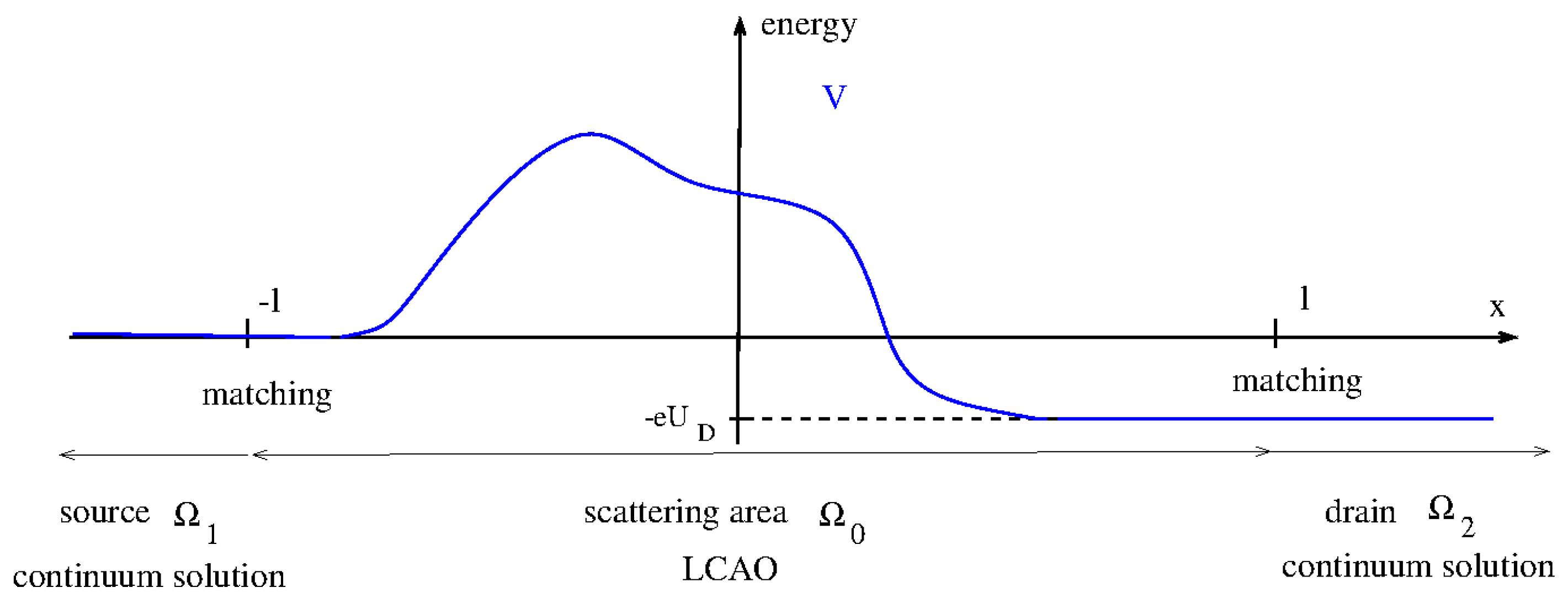
In a 1d-slab model all relevant quantities are assumed to be x-dependent only, in particular, $v_{ext}=v_{ext}\left(x\right)$, which implies $n=n\left(x\right)$ as well as ${\rho }_b={\rho }_b\left(x\right)$ [24,25]. In an open system we then take the total potential as a scattering potential of the form

$$V\left(x\right)=v_{ext}\left(x\right)+v_H\left(x\right)+v_{xc}\left(x\right)=\left\{\begin{array}{cc}0\hfill & \mathrm{in} {\mathrm{\Omega }}_1(\mathrm{i}.\mathrm{e}.,x\le -l)\hfill \\ \mathrm{arbitrary}\hfill & \mathrm{in} {\mathrm{\Omega }}_0(\mathrm{i}.\mathrm{e}.,-l\le x\le l)\hfill \\ -e{U}_D\hfill & \mathrm{in} {\mathrm{\Omega }}_2(\mathrm{i}.\mathrm{e}.,x\ge l),\hfill \end{array}\right.$$

(15)

where ${\mathrm{\Omega }}_0$ is the scattering area (see Figure 1). We assume identical contacts located in ${\mathrm{\Omega }}_1$ (source) and ${\mathrm{\Omega }}_2$ (drain) so that the potential difference $-e{U}_D$ between them corresponds to the applied drain voltage $U_D$. We specify the three potential factors in (15):

-

Hartree potential $v_H$: In the continuum model we solve the 1d Poisson equation

$${\displaystyle \frac{d^2}{d{x}^2}}{v}_H\left(x\right)={\displaystyle \frac{e}{{\kappa }_0\kappa }}\rho \left(x\right)$$

(16)

in ${\mathrm{\Omega }}_0$ with inhomogeneous Dirichlet boundary conditions

$$v_H(-l)=0\mathrm{and}{v}_H\left(l\right)=-e{U}_D.$$

(17)

In Ref. [26] it is derived that

$$v_H(-l\le x\le l)={\displaystyle \frac{e}{{\kappa }_0\kappa }}{\int }_{-l}^l\left({\displaystyle \frac{1}{2}}|x-x^{\prime }|+{\displaystyle \frac{1}{2l}}x{x}^{\prime }-{\displaystyle \frac{l}{2}}\right)\rho \left(x^{\prime }\right)d{x}^{\prime }-e{U}_D{\displaystyle \frac{x+l}{2l}}.$$

(18)

We assume that $x=\pm l$ lies well in the bulk of the contacts so that $\rho \left(\right|x|>l)=0$ and we can set

$$v_H(x\le -l)=0\mathrm{and}{v}_H(x>l)=-e{U}_D$$

(19)

preserving the continuity of $v_H$ at $x=\pm l$. In Ref. [26] it was found that in a self-consistent Hartree-theory the density adjusts in the iterations so that

$$v_H^{\prime }(-l^{+})=v_H^{\prime }\left(l^{-}\right)\to 0.$$

(20)

Consequently, the derivative of $v_H$ also becomes continuous at $x=\pm l$.

-

Exchange-correlation potential $v_{xc}$: Because of the local charge neutrality in the contacts, one obtains from (10)

$$f\left(n\left(x\right)\right)=f\left(n_0\right)\mathrm{for}\left|x\right|\ge l,$$

(21)

where in the contacts we write $n(x\le -l)=n(x\ge l)\equiv n_0$. From (11) it follows

$$v_{xc}^{\mathrm{LDA}}\left(\right|x|\ge l)=f^{\prime }\left(n_0\right).$$

(22)

-

External potential $v_{ext}$: It is convenient to define in the identical contacts for the energy of the conduction band $v_{off}\left(\right|x|\ge l)=-f^{\prime }\left(n_0\right)$ so that Equation (15) holds. In the scattering area the offset potentials are chosen such that their jumps correspond to the correct values.

Figure 1. Kohn–Sham potential for an open system in one dimension. The effective Kohn–Sham potential exhibits the asymptotic behavior $V(x\le -l)=0$ and $V(x\ge l)=-e{U}_D$ (blue line).

Figure 1. Kohn–Sham potential for an open system in one dimension. The effective Kohn–Sham potential exhibits the asymptotic behavior $V(x\le -l)=0$ and $V(x\ge l)=-e{U}_D$ (blue line).

In the 1d slab model, Kohn–Sham Equation (1) becomes

$$\begin{array}{ccc}& & \left[-{\displaystyle \frac{{\hslash }^2}{2m}}{\displaystyle \frac{d^2}{d{x}^2}}+V\left(x\right)-E_x\right]\psi (x,E_x)=0\hfill \\ & \iff & \left[{\displaystyle \frac{d^2}{d{x}^2}}+ϵ-v\left(x\right)\right]\psi (x,ϵ)=0,\hfill \end{array}$$

(23)

where we write

$${\varphi }_{\lambda }\left(\overrightarrow{r}\right)={\displaystyle \frac{\exp (i{k}_{y}y+i{k}_{z}z)}{\sqrt{L_y{L}_z}}}\psi (x,ϵ).$$

(24)

Here $E_x=E_{\lambda }-{\hslash }^2(k_y^2+k_z^2)/\left(2m\right)$ is the energy of the motion in the x-direction, $ϵ=2m{E}_x/{\hslash }^2$, $v\left(x\right)=2mV\left(x\right)/{\hslash }^2$, and $\lambda =(ϵ,k_y,k_z)$. In the scattering potential the source-incident scattering states ${\mathrm{\Psi }}^S$ are defined through the asymptotics

$${\psi }^S(x,ϵ)\equiv {\psi }^S(x,k_L)=\left\{\begin{array}{cc}\exp [i{k}_L(x+l)+r\exp [-i{k}_L(x+l)]\hfill & \mathrm{for} x\le -l\hfill \\ t\exp \left[i{k}_R(x-l)\right]\hfill & \mathrm{for} x\ge l\hfill \end{array}\right.$$

(25)

with $k_L=\sqrt{ϵ}$ and $k_R=\sqrt{ϵ+2me{U}_D/{\hslash }^2}$. For the drain-incident scattering states ${\psi }^D$ an analogous expression holds.

The zero temperature density functional theory of Hohenberg, Kohn and Sham has been generalized for finite temperatures by Mermin [27], introducing the temperature-dependent functional for the grand canonical total potential. By taking the variational derivative with respect to the density we obtain a temperature-dependent effective potential for the Kohn–Sham equations. In the temperature-dependent theory, the occupation of the Kohn–Sham orbitals is given by the Fermi–Dirac distribution so that instead of (9) we write for the carrier density

$$n\left(\overrightarrow{r}\right)=\sum _{\lambda }{f}_{FD}(E_{\lambda }-{\mu }_{\lambda }){\left|{\varphi }_{\lambda }\left(\overrightarrow{r}\right)\right|}^2$$

(26)

with the Fermi–Dirac statistic $f_{FD}(E-\mu )={[e^{(E-\mu )/\left(k_{B}T\right)}+1]}^{-1}$. Following the standard assumption of the Landuer–Büttiker formalism the chemical potential of the source-incident scattering state is given by the chemical potential of the isolated source contact, which is usually taken as grounded, ${\mu }_{\lambda }=\mu$. The chemical potential of the (identical) isolated drain contact is lowered by the drain voltage by $e{U}_D$ so that for drain-incident scattering states ${\mu }_{\lambda }=\mu -e{U}_D$. It should be noted that within this framework, an equilibrium LDA exchange-correlation functional is evaluated on a non-equilibrium Landauer–Büttiker carrier density. Consequently, genuine non-equilibrium exchange-correlation effects—such as the dependence of the functional on net currents or velocity distributions—are neglected. The assignment of different reservoir chemical potentials ${\mu }_{\lambda }$ to individual scattering states accounts for boundary driving conditions but does not inherently capture these intrinsic non-equilibrium corrections. In the following, we assume the temperature is low enough, ($k_{B}T\ll E_F$), to take the zero temperature limit (2) of the Kohn–Sham potential while still using (26) to calculate the carrier density. Inserting Equation (25) in (26), one finds

$$\begin{array}{ccc}\hfill n\left(x\right)& =& {\displaystyle \frac{1}{L_y{L}_z}}\sum _{k_L,k_y,k_z}{f}_{FD}[E(k_L,k_y,k_z)-\mu ]{\left|{\psi }^S(x,k_L)\right|}^2\hfill \\ & & +{\displaystyle \frac{1}{L_y{L}_z}}\sum _{k_R,k_y,k_z}{f}_{FD}[E(k_R,k_y,k_z)-(\mu -e{U}_D)]{\left|{\psi }^D(x,k_R)\right|}^2,\hfill \end{array}$$

(27)

where $E\left(k_{L/R,k_y,k_z}\right)=[{\hslash }^2/\left(2m\right)](k_{L/R}^2+k_y^2+k_z^2)$. In the open system $k_{L/R}$ is a continuum and the sum over $k_{L/R}$ transforms into an integral. As discussed in Appendix A of [4], we can replace ${\sum }_{k_{L/R}}\to (1/\pi ){\int }_0^{\infty }d{k}_{L/R}$ where a spin factor of 2 is included. Then Equation (27) becomes (including spin) for the contribution of the source-incident states to the carrier density

$$\begin{array}{ccc}\hfill n^S\left(x\right)& =& {\displaystyle \frac{1}{\pi L_y{L}_z}}\sum _{k_y,k_z}{\int }_0^{\infty }dk{f}_{FD}\left[E(k,k_y,k_z)\right]{\left|{\psi }^S(x,k)\right|}^2\hfill \\ & =& {\displaystyle \frac{1}{\pi }}{\displaystyle \frac{1}{{\left(2\pi \right)}^2}}{\int }_0^{\infty }d{k}_y\int d{k}_z{\int }_0^{\infty }dk{f}_{FD}\left[E(k,k_y,k_z)\right]{\left|{\psi }^S(x,k)\right|}^2\hfill \\ & =& {\displaystyle \frac{1}{4{\pi }^3}}{\int }_0^{\infty }dk{\left|{\psi }^S(x,k)\right|}^2\left[{\int }_0^{\infty }d{k}_y\int d{k}_z{f}_{FD}\left[E(k,k_y,k_z)\right]\right]\hfill \\ & =& {\displaystyle \frac{1}{4{\pi }^3}}{\int }_0^{\infty }dk{S}_L\left[E_x\left(k\right)\right]{\left|{\psi }^S(x,k)\right|}^2,\hfill \end{array}$$

(28)

where we write $k_{L/R}\to k$. The total energy is split into longitudinal and transverse components: $E=E_x+E_{\perp }={\displaystyle \frac{{\hslash }^2{k}^2}{2m}}+{\displaystyle \frac{{\hslash }^2{k}_{\perp }^2}{2m}}$ where $k_{\perp }^2=k_y^2+k_z^2$. Transforming the transverse double integral into polar coordinates ($d{k}_{y}d{k}_z=\pi d\left(k_{\perp }^2\right)$) yields

$$S_L\left(E_x\right)=\pi {\int }_0^{\infty }d\left(k_{\perp }^2\right){\displaystyle \frac{1}{\exp \left(\frac{\frac{{\hslash }^2{k}_{\perp }^2}{2m}+E_x-\mu }{k_{B}T}\right)+1}}.$$

(29)

We now substitute the dimensionless variable $v={\displaystyle \frac{{\hslash }^2{k}_{\perp }^2}{2m{k}_{B}T}}$ (hence $d\left(k_{\perp }^2\right)={\displaystyle \frac{2m{k}_{B}T}{{\hslash }^2}}dv$) and define the auxiliary variable $y={\displaystyle \frac{\mu -E_x}{k_{B}T}}$. The transverse integral then evaluates to

$$\pi \left({\displaystyle \frac{2m{k}_{B}T}{{\hslash }^2}}\right){\int }_0^{\infty }dv{\displaystyle \frac{1}{\exp (v-y)+1}}={\displaystyle \frac{2\pi m{k}_{B}T}{{\hslash }^2}}\ln \left(1+\exp \left({\displaystyle \frac{\mu -E_x}{k_{B}T}}\right)\right)$$

(30)

and thus

$$S_L\left(E_x\right)={\displaystyle \frac{2\pi m{k}_{B}T}{{\hslash }^2}}\ln \left(1+\exp \left({\displaystyle \frac{\mu -E_x}{k_{B}T}}\right)\right)\equiv S\left(E_x\right).$$

(31)

For the contribution of the drain incident-scattering states we analogously obtain

$$S_R\left(E_x\right)={\displaystyle \frac{2\pi m{k}_{B}T}{{\hslash }^2}}\ln \left(1+\exp \left({\displaystyle \frac{\mu -e{U}_D-E_x}{k_{B}T}}\right)\right)=S(E_x+e{U}_D).$$

(32)

3. R-Matrix Theory for the Schrödinger–(Kohn–Sham) Equation in the Weak Formulation

Adopting the notations of [16], we here cast the R-matrix theory for the Schrödinger– (Kohn–Sham) Equation (23) in the weak formulation. The central results are the expansion of the wave functions and the carrier density in the Wigner–Eisenbud basis in Section 3.2 and Section 3.3. This expression for the carrier density has the practical advantage that the necessary energy integration is space-independent, which is crucial for applying the density functional theory.

3.1. The Wigner–Eisenbud Functions and -Energies in the Lagrange Basis

The Wigner–Eisenbud functions (WE-functions) are the normalized solutions of the eigenvalue problem associated with (23)

$$\begin{array}{c}\hfill \left[{\displaystyle \frac{d^2}{d{x}^2}}-v\left(x\right)+{ϵ}_i\right]{\chi }_i\left(x\right)=0,\end{array}$$

(33)

with homogeneous Neumann boundary conditions.

$${\left.{\displaystyle \frac{d{\chi }_i}{dx}}\right|}_{-l}={\left.{\displaystyle \frac{d{\chi }_i}{dx}}\right|}_l=0.$$

(34)

The WE-functions constitute a complete and orthonormal system of real functions and we can write for a general solution of (23)

$$\psi (x,ϵ)={\displaystyle \sum _{i=1}^n}{a}_i{\chi }_i\left(x\right)$$

(35)

with the expansion coefficients given by

$$a_i={\int }_{-l}^{l}dx\psi (x,ϵ){\chi }_i\left(x\right).$$

(36)

To construct a weak solution of (33) we introduce a set of n test functions ${\mathrm{\Phi }}_j$, $j=1\dots n$, multiplying the equation by a given test function and integrating by parts thereby yields

$${\int }_{-l}^{l}dx{\mathrm{\Phi }}_j^{\prime }\left(x\right){\chi }_i^{\prime }\left(x\right)+{\int }_{-l}^{l}dx{\mathrm{\Phi }}_j\left(x\right)v\left(x\right){\chi }_i\left(x\right)={ϵ}_i{\int }_{-l}^{l}dx{\mathrm{\Phi }}_j\left(x\right){\chi }_i\left(x\right).$$

(37)

Because of the homogeneous Neumann boundary conditions the boundary terms of the integration by parts vanish. In the interior domain ${\mathrm{\Omega }}_0=[-l,l]$ each WE-function ${\chi }_i\left(x\right)$ is then approximated as a linear combination of the basis functions,

$${\chi }_i\left(x\right)={\displaystyle \sum _{j=1}^n}{u}_i^j{\mathrm{\Phi }}_j\left(x\right)$$

(38)

with the coefficient vector ${\mathbf{u}}_i={(u_i^1,\dots ,u_i^n)}^T$. Substituting this ansatz in (37) leads to a generalized matrix eigenvalue problem

$$\mathbf{h}{\mathbf{u}}_i={ϵ}_i\mathbf{b}{\mathbf{u}}_i$$

(39)

with the real, symmetrical $n\times n$ Hamilton matrix

$$h_{j{j}^{\prime }}={\int }_{-l}^{l}dx\left[{\mathrm{\Phi }}_j^{\prime }\left(x\right){\mathrm{\Phi }}_{j^{\prime }}^{\prime }\left(x\right)+v\left(x\right){\mathrm{\Phi }}_{j^{\prime }}\left(x\right){\mathrm{\Phi }}_j\left(x\right)\right]$$

(40)

and the likewise real, symmetrical $n\times n$ overlap matrix

$$b_{j{j}^{\prime }}={\int }_{-l}^{l}dx{\mathrm{\Phi }}_j\left(x\right){\mathrm{\Phi }}_{j^{\prime }}\left(x\right).$$

(41)

The generalized eigenvalue problem (39) thus has n real solutions $u_i^j$ with real eigenvalues ${ϵ}_i$. As the most important application, we assume Lagrange test functions ${\mathrm{\Phi }}_j\left(x\right)$, which are centered around n nodes $x_j$, requiring

$${\mathrm{\Phi }}_{j^{\prime }}\left(x_j\right)={\delta }_{j{j}^{\prime }}.$$

(42)

Then, for sufficiently smooth potentials one obtains

$$v_{j{j}^{\prime }}={\int }_{-l}^{l}dx{\mathrm{\Phi }}_j\left(x\right)v\left(x\right){\mathrm{\Phi }}_{j^{\prime }}\left(x\right)\sim {\int }_{-l}^{l}dx{\mathrm{\Phi }}_j\left(x\right){\displaystyle \frac{v\left(x_j\right)+v\left(x_{j^{\prime }}\right)}{2}}{\mathrm{\Phi }}_{j^{\prime }}\left(x\right)={\displaystyle \frac{v\left(x_j\right)+v\left(x_{j^{\prime }}\right)}{2}}{b}_{j{j}^{\prime }}.$$

(43)

Therefore, in this approximation, the potential has to be known only at the grid points $x_j$. As discussed in detail in Section 5 of Ref. [16], within this approach, the ${\mathrm{\Phi }}_j$ can be chosen as linear Lagrange elements (’hat functions’) to generate the classical finite element method. Non-linear Lagrange elements generate the spectral element method [22,23].

3.2. Calculation of the Wave Functions

Analogous to (38), we write for the wave function

$$\psi (x,ϵ)={\displaystyle \sum _{j=1}^n}{\mathrm{\Psi }}_j{\mathrm{\Phi }}_j\left(x\right)$$

(44)

where we introduce the vector of the expansion coefficients $\mathbf{\Psi }={({\mathrm{\Psi }}_1,\dots ,{\mathrm{\Psi }}_n)}^T$. To obtain a matrix equation like (39) for the wave function we start from Schrödinger Equation (23), multiply with a given basis function, integrate by parts and insert (44) to find the matrix equation

$$(\mathbf{h}-ϵ\mathbf{b})\mathbf{\Psi }={\mathbf{f}}_{\mathrm{boundary}}.$$

(45)

The boundary source vector ${\mathbf{f}}_{\mathrm{boundary}}$ results from the evaluation terms at the system boundaries. Assuming ${\mathrm{\Phi }}_1(-l)={\mathrm{\Phi }}_n\left(l\right)=1$ and (42) one finds

$${\mathbf{f}}_{\mathrm{boundary}}={\left(-{\mathrm{\Psi }}^{\prime }(-l),0,\dots ,0,{\mathrm{\Psi }}^{\prime }\left(l\right)\right)}^T.$$

(46)

Introducing the b-orthogonal modal matrix $\mathbf{U}=({\mathbf{u}}_1,\dots ,{\mathbf{u}}_n)$, we demonstrate in Appendix B that the formal solution of (45) reads

$$\mathbf{\Psi }=\mathbf{U}\mathrm{diag}\left({\displaystyle \frac{1}{{ϵ}_i-ϵ}}\right){\mathbf{U}}^T{\mathbf{f}}_{\mathrm{boundary}}.$$

(47)

Because of the sparse character of ${\mathbf{f}}_{\mathrm{boundary}}$ in (46) one finds the two equations

$$\begin{array}{cc}\hfill {\mathrm{\Psi }}_1& =R_{11}{\mathrm{\Psi }}^N(-l)+R_{12}{\mathrm{\Psi }}^N\left(l\right)\hfill \end{array}$$

(48)

$$\begin{array}{cc}\hfill {\mathrm{\Psi }}_n& =R_{21}{\mathrm{\Psi }}^N(-l)+R_{22}{\mathrm{\Psi }}^N\left(l\right)\hfill \end{array}$$

(49)

with

$$R_{s{s}^{\prime }}={\displaystyle \sum _{i=1}^n}{\displaystyle \frac{u_i^{j\left(s\right)}{u}_i^{j\left(s^{\prime }\right)}}{{ϵ}_i-ϵ}}\mathrm{with}s,s^{\prime }\in \{1,2\}\mathrm{and}j\left(1\right)=1,j\left(2\right)=n$$

(50)

and the surface normal derivative defined by ${\mathrm{\Psi }}^N(-l)=-{\mathrm{\Psi }}^{\prime }(-l)$ and ${\mathrm{\Psi }}^N\left(l\right)={\mathrm{\Psi }}^{\prime }\left(l\right).$ From the contact asymptotics of the scattering states in Equation (25) it follows for the source-incident scattering states that

$$\begin{array}{ccc}\hfill & {\mathrm{\Psi }}_1=1+r\hfill & \hfill {\mathrm{\Psi }}^{\prime }(-l)=i{k}_L(1-r)\end{array}$$

(51)

$$\begin{array}{ccc}\hfill & {\mathrm{\Psi }}_n=t\hfill & \hfill {\mathrm{\Psi }}^{\prime }\left(l\right)=i{k}_{R}t.\end{array}$$

(52)

Substituting these expressions into the boundary equations eliminates the boundary values and leads to the closed $2\times 2$ linear system of equations for the unknown scattering coefficients

$$\left(\begin{array}{cc}1-i{k}_L{R}_{11}& -i{k}_R{R}_{12}\\ -i{k}_L{R}_{21}& 1-i{k}_R{R}_{22}\end{array}\right)\left(\begin{array}{c}r\\ t\end{array}\right)=-\left(\begin{array}{c}1+i{k}_L{R}_{11}\\ i{k}_L{R}_{21}\end{array}\right).$$

(53)

This system is solved algebraically for r and t. Once the complex scalars r and t are known we can specify in (46) for the source-incident states

$${\mathbf{f}}_{\mathrm{boundary}}={\left(-i{k}_L(1-r),0,\dots ,0,i{k}_{R}t\right)}^T.$$

(54)

The step-by-step evaluation can be implemented directly without explicit matrix–matrix products:

• Projection onto the modal basis: Calculation of the effective modal excitation $b_i$ for each mode i:

  $$b_i=u_i^1{f}_{\mathrm{boundary},1}+u_i^n{f}_{\mathrm{boundary},n}$$

  (55)
• Spectral resonance filtering: Weighting in the spectral domain:

  $${\tilde{b}}_i={\displaystyle \frac{b_i}{{ϵ}_i-ϵ}}$$

  (56)
• Back-transformation into real space: Summation to yield the physical wave function for each grid node j:

  $${\mathrm{\Psi }}_j={\displaystyle \sum _{i=1}^n}{u}_i^j{\tilde{b}}_i.$$

  (57)

A major advantage of the present formulation over that in [16] is that it avoids the construction of the matrix $g_{ij}$, which is constructed in Equation (21) of latter reference by inversion.

3.3. Construction of the Carrier Density

Inserting the expansions (38) and (44) in (36), one finds

$$a_i={\displaystyle \sum _{j{j}^{\prime }=1}^n}{\mathrm{\Psi }}_j{u}_i^{j^{\prime }}\left({\int }_{-l}^{l}dx{\mathrm{\Phi }}_j\left(x\right){\mathrm{\Phi }}_{j^{\prime }}\left(x\right)\right)={\mathbf{\Psi }}^T\mathbf{b}{\mathbf{u}}_i.$$

(58)

By collecting all eigenvectors ${\mathbf{u}}_i$ as columns into a modal matrix $\mathbf{U}$, the entire coefficient vector $\mathbf{a}={(a_1,\dots ,a_n)}^T$ can be compactly computed via

$$\mathbf{a}={\mathbf{U}}^T\mathbf{b}\mathbf{\Psi }$$

(59)

with

$$a_i=i{\displaystyle \frac{k_R{\chi }_i\left(l\right)t-k_L{\chi }_i(-l)(1-r)}{{ϵ}_i-ϵ}}.$$

(60)

As shown in Appendix A this equation is identical with its counterpart (A9) in strong formulation. From (35) one has

$$\begin{array}{ccc}\hfill |{\psi }^S{(x,ϵ)|}^2& =& \sum _{i{i}^{\prime }}{a}_i^{\ast }\left(ϵ\right)a_{i^{\prime }}\left(ϵ\right){\chi }_i\left(x\right){\chi }_{i^{\prime }}\left(x\right)\hfill \\ & =& \sum _{i{i}^{\prime }}{\displaystyle \frac{k_R{\chi }_i\left(l\right)t^{\ast }-k_L{\chi }_i(-l)(1-r^{\ast })}{{ϵ}_i-ϵ}}{\displaystyle \frac{k_R{\chi }_{i^{\prime }}\left(l\right)t-k_L{\chi }_{i^{\prime }}(-l)(1-r)}{{ϵ}_{i^{\prime }}-ϵ}}{\chi }_i\left(x\right){\chi }_{i^{\prime }}\left(x\right)\hfill \\ & =& \sum _{i{i}^{\prime }}{\gamma }_{i{i}^{\prime }}^S\left(ϵ\right){\chi }_i\left(x\right){\chi }_{i^{\prime }}\left(x\right)\hfill \end{array}$$

(61)

with

$${\gamma }_{i{i}^{\prime }}^S\left(ϵ\right)=a_i^{\ast }\left(ϵ\right)a_{i^{\prime }}\left(ϵ\right)=\left({\displaystyle \frac{k_R{\chi }_i\left(l\right)t^{\ast }-k_L{\chi }_i(-l)(1-r^{\ast })}{{ϵ}_i-ϵ}}\right)\left({\displaystyle \frac{k_R{\chi }_{i^{\prime }}\left(l\right)t-k_L{\chi }_{i^{\prime }}(-l)(1-r)}{{ϵ}_{i^{\prime }}-ϵ}}\right)$$

(62)

Using $dk=dϵ/\left(2{ϵ}^{1/2}\right)$ we can now find from (28) the desired expansion of the carrier density in pairs of Wigner–Eisenbud functions

$$\begin{array}{ccc}\hfill n^S\left(x\right)& =& {\displaystyle \frac{1}{8{\pi }^3}}{\int }_0^{\infty }dϵ{\displaystyle \frac{1}{\sqrt{ϵ}}}S\left(ϵ\right){\left|{\psi }^S(x,ϵ)\right|}^2\hfill \\ & =& {\displaystyle \frac{1}{8{\pi }^3}}\sum _{i{i}^{\prime }}{\int }_0^{\infty }dϵ{\displaystyle \frac{1}{\sqrt{ϵ}}}S\left(ϵ\right){\gamma }_{i{i}^{\prime }}^S\left(ϵ\right){\chi }_i\left(x\right){\chi }_{i^{\prime }}\left(x\right)\hfill \\ & =& \sum _{i{i}^{\prime }}{n}_{i{i}^{\prime }}^S\left(ϵ\right){\chi }_i\left(x\right){\chi }_{i^{\prime }}\left(x\right),\hfill \end{array}$$

(63)

with the expansion coefficients given by

$$n_{i{i}^{\prime }}^S\left(ϵ\right)={\displaystyle \frac{1}{8{\pi }^3}}{\int }_0^{\infty }dϵ{\displaystyle \frac{1}{\sqrt{ϵ}}}S\left(ϵ\right){\gamma }_{i{i}^{\prime }}^S\left(ϵ\right).$$

(64)

Evidently, the energy integration does not depend on x any more. Making use of the nodal properties (42) of the Lagrange elements and inserting further (38) in (63) one obtains

$$n^S\left(x_j\right)=\sum _{i{i}^{\prime }}{n}_{i{i}^{\prime }}^S{u}_i^j{u}_{i^{\prime }}^j.$$

(65)

For the drain-incident scattering states one finds analogous expression $n^D\left(x_j\right)={\sum }_{i{i}^{\prime }}{n}_{i{i}^{\prime }}^D{u}_i^j{u}_{i^{\prime }}^j$. The total electron–particle density at the nodes is thus given by

$$n\left(x_j\right)=n^S\left(x_j\right)+n^D\left(x_j\right)=\sum _{i{i}^{\prime }}{n}_{i{i}^{\prime }}{u}_i^j{u}_{i^{\prime }}^j$$

(66)

with $n_{i{i}^{\prime }}=n_{i{i}^{\prime }}^S+n_{i{i}^{\prime }}^D$.

3.4. Cut-Off in the Wigner–Eisenbud Function Basis

When in numerical calculations a finite number n of basis functions is used, only the lowest $N<n$ Wigner–Eisenbud functions will be correct. Introducing the technique proposed by Buttle [28] we write (61) as

$$\begin{array}{ccc}& & {\left|\psi (ϵ,x)\right|}^2=\sum _{i{i}^{\prime }}{\displaystyle \frac{k_R{\chi }_i\left(l\right)t^{\ast }-k_L{\chi }_i(-l)(1-r^{\ast })}{{ϵ}_i-ϵ}}{\displaystyle \frac{k_R{\chi }_{i^{\prime }}\left(l\right)t-k_L{\chi }_{i^{\prime }}(-l)(1-r)}{{ϵ}_{i^{\prime }}-ϵ}}{\chi }_i\left(x\right){\chi }_{i^{\prime }}\left(x\right)\hfill \\ & \sim & \left\{\left[{\rho }_{12}(ϵ,x)+{\rho }_{12}^{rest}(ϵ,x)\right]t^{\ast }-\left[{\rho }_{11}(ϵ,x)+{\rho }_{11}^{rest}(ϵ,x)\right](1-r^{\ast })\right\}\hfill \\ & & \times \left\{\left[{\rho }_{12}(ϵ,x)+{\rho }_{12}^{rest}(ϵ,x)\right]t-\left[{\rho }_{11}(ϵ,x)+{\rho }_{11}^{rest}(ϵ,x)\right](1-r)\right\}\hfill \end{array}$$

(67)

with

$${\rho }_{12}(ϵ,x)=k_R{\displaystyle \sum _{i=1}^N}{\displaystyle \frac{{\chi }_i\left(l\right){\chi }_i\left(x\right)}{{ϵ}_i-ϵ}},$$

(68)

$${\rho }_{11}(ϵ,x)=k_L{\displaystyle \sum _{i=1}^N}{\displaystyle \frac{{\chi }_i(-l){\chi }_i\left(x\right)}{{ϵ}_i-ϵ}},$$

(69)

$${\rho }_{12}^{rest}(E,x)=k_R{\displaystyle \sum _{i=N+1}^{\infty }}{\displaystyle \frac{{\chi }_i^0\left(l\right){\chi }_i^0\left(x\right)}{{ϵ}_i^0-ϵ}},$$

(70)

and

$${\rho }_{11}^{rest}(ϵ,x)=k_L{\displaystyle \sum _{i=N+1}^{\infty }}{\displaystyle \frac{{\chi }_i^0(-l){\chi }_i^0\left(x\right)}{{ϵ}_i^0-ϵ}}.$$

(71)

Here the ${\chi }_i^0$ and ${ϵ}_i^0$ are the Wigner–Eisenbud functions and energies for $v\left(x\right)$ replaced by the constant $\left[{\int }_{-l}^{l}dxv\left(x\right)\right]/\left(2l\right)$.

3.5. Resonant Tunneling

The space-independent nature of the integration in Equation (64) is particularly advantageous for devices featuring strong confinement or sharp transmission resonances, such as resonant tunneling structures. In such systems, evaluating the carrier density using traditional grid-bound techniques requires an exceptionally fine energy mesh ($N_E\gg 1$) at each individual spatial node to accurately capture the peak profiles, leading to a severe numerical bottleneck. In our formulation, this fine integration is performed only once globally for the coefficients $n_{i{i}^{\prime }}$. Furthermore, near a sharp resonance, the transport is typically dominated by a single Wigner–Eisenbud level. Consequently, the diagonal matrix element $n_{ii}$ for this specific mode contains the overwhelming majority of the total carrier charge, while the off-diagonal cross-terms remain negligible. This physical property allows for a truncation of the spectral sum where off-diagonal cross-terms are expected to be negligible.

4. Self-Consistency Loop: Poisson Equation in Weak Formulation

In the previous section the wave functions and the quantum electron density n were constructed in the weak formulation if the Kohn–Sham potential $V=v_{ext}+v_H+v_{xc}$ in the LDA was known. In this section we assume, in addition, that if the potential is given, the positive background charge density ${\rho }_b$ can also be calculated so that the global charge neutrality holds.

$${\int }_{-l}^l\rho \left(x\right)dx=0\mathrm{with}\rho \left(x\right)=-en\left(x\right)+{\rho }_b$$

(72)

Here $n\left(x\right)$ is the contribution of the free current-carrying charge carriers in the energy continuum of scattering states with $ϵ\ge 0$. It is given by Equations (63) and (64).

Under certain conditions bound electronic states with $ϵ<0$ may be of physical relevance for strongly populated conduction channels, for example, in the two-channel transistor with a back and front gate [10]. Such states can be included in our approach by incorporating the electron density of the bound states directly into the background charge profile. Consequently, we neglect the specific exchange-correlation corrections that these bound electrons would rigorously contribute to the exchange-correlation functional $E_{xc}^{LDA}\left[n\right]$. To bypass the problem of the non-equilibrium occupation of the bound states one assumes full occupation of the bound states. The contribution of the bound charge carriers to ${\rho }_b$ can then be calculated from the sum of the squares of the Wigner–Eisenbud functions with negative energies if the l chosen is large enough. Because of their exponential decay, these Wigner–Eisenbud functions and their derivatives become close to zero at $x=\pm l$. The global charge neutrality in Equation (72) is an immediate consequence of charge conservation because of the charge neutrality in the contacts, $\rho \left(\right|x|>l)=0$. In the self-consistency loop, in turn, the Kohn–Sham potential V is updated once n and ${\rho }_b$ are known. Here the band offset potential $v_{ext}$ is fixed and the exchange-correlation potential follows immediately by insertion of Equations (63) and (64) in $v_{xc}\left(n\right)$. The remaining Hartree-term obeys the Poisson Equation (73)

$${\displaystyle \frac{d^2}{d{x}^2}}{v}_H\left(x\right)={\displaystyle \frac{e}{\kappa {\kappa }_0}}\rho \left(x\right),$$

(73)

where $v_H$ is the energy of the negative electron. On the finite interval $x\in [-l,l]$ we impose the inhomogeneous Dirichlet boundary conditions

$$v_H(-l)=0\mathrm{and}{v}_H\left(l\right)=-e{U}_D.$$

(74)

In weak formulation we write

$${\int }_{-l}^l{\mathrm{\Phi }}_j\left(x\right){\displaystyle \frac{d^2{v}_H\left(x\right)}{d{x}^2}}={\int }_{-l}^l{\mathrm{\Phi }}_j\left(x\right){\displaystyle \frac{e}{\kappa {\kappa }_0}}\rho \left(x\right)\equiv r_j.$$

(75)

For the expansion of the Hartree potential

$$v_H\left(x\right)={\displaystyle \sum _{j=1}^n}{v}_H^j{\mathrm{\Phi }}_j\left(x\right)$$

(76)

we take the same localized Lagrange elements ${\mathrm{\Phi }}_j\left(x\right)$ as in (38) of Section 3.1. The nodal property ${\mathrm{\Phi }}_{j^{\prime }}\left(x_j\right)={\delta }_{j{j}^{\prime }}$ of the Lagrange elements allows for the enforcement of the Dirichlet boundary conditions (74) by specifying now $x_1=-l$ as well as $x_n=l$ and by fixing in (76)

$$0=v_H^1\mathrm{and}-e{U}_D=v_H^n.$$

(77)

Moreover, a unified basis for the quantum transport and the electrostatic solver eliminates the need for a basis transformation, thereby avoiding potential errors. Partial integration on the l.h.s. of (75) yields n equations

$${\mathrm{\Phi }}_j\left(l\right)v_H^{\prime }\left(l\right)-{\mathrm{\Phi }}_j(-l)v_H^{\prime }(-l)-{\int }_{-l}^{l}dx{\mathrm{\Phi }}_j^{\prime }\left(x\right)v_H^{\prime }\left(x\right)=r_j.$$

(78)

Because of the boundary conditions (77) one obtains $n-2$ inhomogeneous equations

$$-{\int }_{-l}^{l}dx{\mathrm{\Phi }}_j^{\prime }\left(x\right)v_H^{\prime }\left(x\right)=r_j$$

(79)

for the $n-2$ unknowns $v_H^2\dots v_H^{n-1}$ where we have taken into account the relation ${\mathrm{\Phi }}_{j^{\prime }}\left(x_j\right)={\delta }_{j{j}^{\prime }}$ for modal elements $j^{\prime }=2\dots n-1$ at $x_1$ and $x_n$. Inserting the derivative of (76) one has

$$-{\displaystyle \sum _{j^{\prime }=2}^{n-1}}{\beta }_{j{j}^{\prime }}{v}_H^{j^{\prime }}=r_j+{\beta }_{jn}(-e{U}_D)\equiv R_j$$

(80)

with the stiffness matrix

$${\beta }_{j{j}^{\prime }}={\int }_{-l}^{l}dx{\mathrm{\Phi }}_j^{\prime }\left(x\right){\mathrm{\Phi }}_{j^{\prime }}^{\prime }\left(x\right).$$

(81)

These are $n-2$ inhomogeneous linear equations for the $n-2$ unknowns $v_H^2\dots v_H^{n-1}$. Graphically,

$$\left(\begin{array}{ccc}{\beta }_{22}& \dots & {\beta }_{2(n-1)}\\ ⋮& ⋮& ⋮\\ {\beta }_{(n-1)2}& \dots & {\beta }_{(n-1)(n-1)}\end{array}\right)\left(\begin{array}{c}{v}_H^2\\ ⋮\\ v_H^{(n-1)}\end{array}\right)=-\left(\begin{array}{c}{R}_2\\ ⋮\\ R_{n-1}\end{array}\right).$$

(82)

As has been demonstrated for the continuum model in Ref. [26], if the l chosen is large enough then

$$v_H^{\prime }(\pm l)\to 0$$

(83)

since the points $\pm l$ are located in the bulk of the contacts where $\rho (\pm l)\to 0$. In contrast, a finite value of $v_H^{\prime }(\pm l)$ would imply a delta-peaked $\rho$ at $x=\pm l$.

To close the self-consistency loop algebraically, the continuous source vector integral $r_j={\displaystyle \frac{e}{\kappa {\kappa }_0}}{\int }_{-l}^l{\mathrm{\Phi }}_j\left(x\right)\rho \left(x\right)dx$ must be evaluated. We approximate the continuous total charge density $\rho \left(x\right)$ by its expansion in the localized Lagrange basis, $\rho \left(x\right)\approx {\sum }_{j^{\prime }=1}^n\rho \left(x_{j^{\prime }}\right){\mathrm{\Phi }}_{j^{\prime }}\left(x\right)$. Substituting this ansatz into the weak formulation integral yields:

$$r_j\approx {\displaystyle \frac{e}{\kappa {\kappa }_0}}{\displaystyle \sum _{j^{\prime }=1}^n}\rho \left(x_{j^{\prime }}\right){\int }_{-l}^l{\mathrm{\Phi }}_j\left(x\right){\mathrm{\Phi }}_{j^{\prime }}\left(x\right)dx={\displaystyle \frac{e}{\kappa {\kappa }_0}}{\displaystyle \sum _{j^{\prime }=1}^n}{b}_{j{j}^{\prime }}\rho \left(x_{j^{\prime }}\right),$$

(84)

where $b_{j{j}^{\prime }}$ is the symmetric $n\times n$ overlap matrix defined in Equation (41). Assuming a smoothly varying charge profile where the nodal value $\rho \left(x_j\right)$ dominates the local spatial tributary area, the summation can be simplified to the standard nodal quadrature approximation:

$$r_j\approx {\displaystyle \frac{e}{\kappa {\kappa }_0}}\rho \left(x_j\right){\displaystyle \sum _{j^{\prime }=1}^n}{b}_{j{j}^{\prime }}.$$

(85)

This algebraic formulation effectively couples the spatial grid charge to the electrostatic solver without requiring a manual basis transformation.

5. Analytical Relation to the Finite Difference Method

To establish a consistency check for the presented weak formulation method and to demonstrate its physical and mathematical connection to established grid-bound techniques, this section shows that the classical finite difference (FD) method emerges as a direct analytic limiting case of our generalized framework. This links the present framework directly to the self-consistent transport scheme of Ref. [26].

5.1. Explicit Basis Functions in the Finite Difference Limit

The standard finite difference formulation in a one-dimensional continuum is mathematically identical to a finite element discretization that employs piecewise linear Lagrange elements (commonly referred to as “hat” or “tent” functions) defined on an equidistant real-space grid.

Let the continuous interval ${\mathrm{\Omega }}_0=[-l,l]$ be partitioned into $n-1$ equal subintervals of length $h=x_{j+1}-x_j$. For any interior node j (where $j=2,\dots ,n-1$), the localized linear basis function ${\mathrm{\Phi }}_j\left(x\right)$ is defined explicitly as

$${\mathrm{\Phi }}_j\left(x\right)=\left\{\begin{array}{cc}{\displaystyle \frac{x-x_{j-1}}{h}}\hfill & \mathrm{for}{x}_{j-1}\le x\le x_j\hfill \\ {\displaystyle \frac{x_{j+1}-x}{h}}\hfill & \mathrm{for}{x}_j\le x\le x_{j+1}\hfill \\ 0\hfill & \mathrm{otherwise}.\hfill \end{array}\right.$$

(86)

These functions satisfy the defining interpolating property ${\mathrm{\Phi }}_j\left(x_{j^{\prime }}\right)={\delta }_{j{j}^{\prime }}$. The first derivative ${\mathrm{\Phi }}_j^{\prime }\left(x\right)$ is piecewise constant within the adjacent mesh cells

$${\mathrm{\Phi }}_j^{\prime }\left(x\right)=\left\{\begin{array}{cc}{\displaystyle \frac{1}{h}}\hfill & \mathrm{for}{x}_{j-1}<x<x_j\hfill \\ -{\displaystyle \frac{1}{h}}\hfill & \mathrm{for}{x}_j<x<x_{j+1}\hfill \\ 0\hfill & \mathrm{otherwise}.\hfill \end{array}\right.$$

(87)

Evaluating the stiffness matrix elements ${\beta }_{j{j}^{\prime }}$ defined in Equation (81) using these explicit derivatives leads to a sparse tridiagonal matrix. For the interior nodes ($j=2,\dots ,n-1$), the integration spans over both adjacent elements so that

$${\beta }_{jj}={\int }_{-l}^l{\left[{\mathrm{\Phi }}_j^{\prime }\left(x\right)\right]}^{2}dx={\int }_{x_{j-1}}^{x_j}{\left({\displaystyle \frac{1}{h}}\right)}^{2}dx+{\int }_{x_j}^{x_{j+1}}{\left(-{\displaystyle \frac{1}{h}}\right)}^{2}dx={\displaystyle \frac{2}{h}},$$

(88)

and for adjacent nodes

$${\beta }_{j,j\pm 1}={\int }_{-l}^l{\mathrm{\Phi }}_j^{\prime }\left(x\right){\mathrm{\Phi }}_{j\pm 1}^{\prime }\left(x\right)dx=-{\displaystyle \frac{1}{h}}.$$

(89)

It is critical to note that at the boundaries ($j=1$ and $j=n$), the basis functions are truncated by the domain boundaries $[-l,l]$. Consequently, the integration only spans a single element, which scales the boundary diagonal elements to

$${\beta }_{11}={\beta }_{nn}={\displaystyle \frac{1}{h}}.$$

(90)

For all non-adjacent nodes ($|j-j^{\prime }|>1$), the overlap of the derivatives vanishes identically, meaning ${\beta }_{j{j}^{\prime }}=0$.

5.2. Explicit Evaluation of the Source Vector $R_j$

First, the primary source contribution $r_j$ from the nodal quadrature approximation in Equation (85) is evaluated. For the piecewise linear Lagrange elements defined on our equidistant grid, the explicit integration of the overlap matrix elements yields $b_{jj}={\displaystyle \frac{2}{3}}h$ and $b_{j,j\pm 1}={\displaystyle \frac{1}{6}}h$. Evaluating the row-sum for any interior node $j=2,\dots ,n-1$ results precisely in the spatial tributary length:

$${\displaystyle \sum _{j^{\prime }=1}^n}{b}_{j{j}^{\prime }}=b_{j,j-1}+b_{jj}+b_{j,j+1}={\displaystyle \frac{1}{6}}h+{\displaystyle \frac{2}{3}}h+{\displaystyle \frac{1}{6}}h=h.$$

(91)

Substituting this geometric result (91) into the localized charge expression yields the non-vanishing, standard discretized source density at each interior node:

$$r_j\approx {\displaystyle \frac{e}{\kappa {\kappa }_0}}\rho \left(x_j\right)·h.$$

(92)

Second, to find $R_j$ via (80), the boundary coupling coefficient ${\beta }_{jn}$ between the interior node j and the rightmost boundary contact node n (located at $x_n=l$) must be evaluated. Due to the strict localization of the linear basis elements, ${\mathrm{\Phi }}_j\left(x\right)$ and ${\mathrm{\Phi }}_n\left(x\right)$ share no common support for any bulk node up to $j=n-2$, giving ${\beta }_{jn}=0$. The sole exception occurs at the node directly adjacent to the drain interface, $j=n-1$, where the overlap integral of the derivatives yields

$${\beta }_{n-1,n}={\int }_{x_{n-1}}^{x_n}{\mathrm{\Phi }}_{n-1}^{\prime }\left(x\right){\mathrm{\Phi }}_n^{\prime }\left(x\right)dx={\int }_{x_{n-1}}^{x_n}\left(-{\displaystyle \frac{1}{h}}\right)\left({\displaystyle \frac{1}{h}}\right)dx=-{\displaystyle \frac{1}{h}}.$$

(93)

Combining these terms, the components of the vector $R_j$ are obtained explicitly as a function of the spatial node position

$$R_j=\left\{\begin{array}{cc}{\displaystyle \frac{e}{\kappa {\kappa }_0}}\rho \left(x_j\right)·h\hfill & \mathrm{for}j=2,\dots ,n-2\hfill \\ {\displaystyle \frac{e}{\kappa {\kappa }_0}}\rho \left(x_{n-1}\right)·h+{\displaystyle \frac{e{U}_D}{h}}\hfill & \mathrm{for}j=n-1.\hfill \end{array}\right.$$

(94)

5.3. Recovery of the Standard Central Difference Stencil

With the explicit expressions for ${\beta }_{j{j}^{\prime }}$ and $R_j$ established, the generalized matrix Equation (80) can be written out row by row for any interior node j

$$-\left({\beta }_{j,j-1}{v}_H^{j-1}+{\beta }_{jj}{v}_H^j+{\beta }_{j,j+1}{v}_H^{j+1}\right)=R_j$$

(95)

For a general bulk node ($j=2,\dots ,n-2$), substituting the explicit coefficients into this line results in

$$-\left(-{\displaystyle \frac{1}{h}}{v}_H^{j-1}+{\displaystyle \frac{2}{h}}{v}_H^j-{\displaystyle \frac{1}{h}}{v}_H^{j+1}\right)={\displaystyle \frac{e}{\kappa {\kappa }_0}}\rho \left(x_j\right)·h$$

(96)

Dividing the entire equation by the grid spacing h yields the exact classical three-point central difference stencil for the second derivative of the Hartree potential

$${\displaystyle \frac{v_H^{j-1}-2v_H^j+v_H^{j+1}}{h^2}}={\displaystyle \frac{e}{\kappa {\kappa }_0}}\rho \left(x_j\right).$$

(97)

For $j=n$ we formally define $v_H^0=0$ because of Equation (15) and write for the latter equation

$${\displaystyle \frac{v_H^0-2v_H^1+v_H^2}{h^2}}={\displaystyle \frac{e}{\kappa {\kappa }_0}}\rho \left(x_j\right).$$

(98)

For $j=1$ we formally define $v_H^{n+1}=-e{U}_D$ because of Equation (15) and write

$${\displaystyle \frac{v_H^{n-1}-2v_H^n+v_H^{n+1}}{h^2}}={\displaystyle \frac{e}{\kappa {\kappa }_0}}\rho \left(x_j\right).$$

(99)

It is worth noting that the recovery of the standard three-point central difference stencil at the very boundaries ($j=1$ and $j=n$) implicitly couples the matrix equations to the boundary derivatives of the Hartree potential. For the leftmost node ($j=1$), the evaluating equation from the weak formulation technically retains the spatial gradient term $v_H^{\prime }(-l)$. The exact equivalence to the standard finite difference expression is mathematically strictly preserved under the condition of a flat potential profile at the contact interfaces, i.e., $v_H^{\prime }(-l)=0$ and $v_H^{\prime }\left(l\right)=0$.

Physically, this condition is fully justified within the open system framework. Since the boundaries $x=\pm l$ are chosen to lie deep within the highly doped, quasi-metallic bulk of the contacts, strong electrostatic screening enforces local charge neutrality, meaning $\rho (\pm l)\to 0$. Consequently, the electric field vanishes at the domain boundaries, forcing the spatial derivatives of the Hartree potential to zero. This physical shielding ensures that the iterative self-consistent loop derived in the weak formulation remains analytically compatible with the grid-bound finite difference scheme across the entire domain.

This analytic proof confirms that the iterative self-consistent loop derived in the weak formulation is mathematically sound, since its linear limiting case is perfectly identical to the standard FD implementation that was successfully executed and benchmarked in Ref. [26], the validity of the underlying physical coupling is established by proxy. While the traditional 1D FD stencil is highly efficient for basic slab models, the strategic utility of casting the system in the weak formulation lies in its immediate extension to multi-dimensional (2D/3D) device grids and higher-order spectral elements without requiring rigid real-space coordinate bindings.

6. Summary

In Section 2 we specify the general density functional theory in the continuum formulation to a 1D slab model in the local density approximation (LDA). The Kohn–Sham equations are derived for current-carrying semiconductor nanostructures with quasi-metallic contacts (highly doped semiconductor beyond the metal-insulator transition). The electron wave functions and the charge density entering the LDA are calculated in the continuum R-matrix theory in Section 2 and Appendix A in strong formulation.

In Section 3 the continuum R-matrix theory for the Kohn–Sham equation is cast in weak formulation. As a major advantage, using Lagrange test functions, the electron wave function and the charge density entering the LDA can be numerically evaluated in the highly effective spectral element method.

In Section 4 the Poisson equation is cast in weak formulation, which also allows the Hartree potential entering the Kohn–Sham equation to be calculated efficiently using the spectral element method as well. It is then easy to construct the total potential entering Kohn–Sham equation.

The results in Section 3 and Section 4 allow us to find a self-consistent solution to the LDA in an iterative procedure.

References

- Nemnes, G.A.; Wulf, U.; Racec, P.N. Nano-transistors in the Landauer-Büttiker formalism. J. Appl. Phys. 2004, 96, 596. [Google Scholar] [CrossRef] [Scilit]
- Nemnes, G.A.; Wulf, U.; Racec, P.N. Nonlinear I-V characteristics of nanotransistors in the Landauer-Büttiker formalism. J. Appl. Phys. 2005, 98, 84308. [Google Scholar] [CrossRef] [Scilit]
- Wulf, U.; Kučera, J.; Richter, H.; Horstmann, M.; Wiatr, M.; Höntschel, J. Channel engineering for nanotransistors in a semiempirical quantum transport model. Mathematics 2017, 5, 68. [Google Scholar] [CrossRef] [Scilit]
- Wulf, U. A One-Dimensional Effective Model for Nanotransistors in Landauer-Büttiker Formalism. Micromachines 2020, 11, 359. [Google Scholar] [CrossRef] [Scilit] [PubMed]
- Kučera, J.; Wulf, U. Scattering Theory in an N-pole semiconductor quantum device: Unitarity of the current S-matrix and current conservation. Micromachines 2025, 16, 306. [Google Scholar] [CrossRef] [Scilit] [PubMed]
- Nemnes, G.A.; Ion, L.; Antohe, S. Self-consistent potentials and linear regime conductance of cylindrical nanowire transistors in the R-matrix formalism. J. Appl. Phys. 2009, 106, 113714. [Google Scholar] [CrossRef] [Scilit]
- Nemnes, G.A.; Manolescu, A.; Gudmundsson, V. Reduction of ballistic spin scattering in a spin-FET using stray electric fields. J. Phys. Conf. Ser. 2012, 338, 012012. [Google Scholar] [CrossRef] [Scilit]
- Nemnes, G.A.; Dragoman, D. Reconfigurable quantum logic gates using Rashba controlled spin polarized currents. Phys. E 2019, 111, 13. [Google Scholar] [CrossRef] [Scilit]
- Wulf, U. An Electron Waveguide Model for FDSOI Transistors. Solids 2022, 3, 203–218. [Google Scholar] [CrossRef] [Scilit]
- Wulf, U.; Preda, A.T.; Nemnes, G.A. Transport in a Two-Channel Nanotransistor Device with Lateral Resonant Tunneling. Micromachines 2024, 15, 1270. [Google Scholar] [CrossRef] [Scilit] [PubMed]
- Kirkner, D.; Lent, C. The quantum transmitting boundary method. J. Appl. Phys. 1990, 67, 6353. [Google Scholar] [CrossRef] [Scilit]
- Leng, M.; Lent, C.S. Recovery of quantized ballistic conductance in a periodically modulated channel. Phys. Rev. Lett. 1993, 71, 137. [Google Scholar] [CrossRef] [Scilit] [PubMed]
- Leng, M.; Lent, C.S. Quantum transmitting boundary method in a magnetic field. J. Appl. Phys. 1994, 76, 2240. [Google Scholar] [CrossRef] [Scilit]
- Leng, M.; Lent, C.S. Conductance quantization in a periodically modulated channel. Phys. Rev. B 1994, 50, 10823. [Google Scholar] [CrossRef] [Scilit] [PubMed]
- Shao, Z.; Porod, W.; Lent, C.S.; Kirkner, D.J. An eigenvalue method for open-boundary quantum transmission problems. J. Appl. Phys. 1995, 78, 2177. [Google Scholar] [CrossRef] [Scilit]
- Wulf, U.; Kučera, J. R-Matrix Theory in a Semiconductor Quantum Device: Weak Formulation and Current Conserving Approximations. Solids 2025, 6, 63. [Google Scholar] [CrossRef] [Scilit]
- Hohenberg, P.; Kohn, W. Inhomogeneous Electron Gas. Phys. Rev. B 1964, 136, B864. [Google Scholar] [CrossRef] [Scilit]
- Kohn, W.; Sham, L.J. Self-Consistent Equations Including Exchange and Correlation Effects. Phys. Rev. A 1965, 140, A1133. [Google Scholar] [CrossRef] [Scilit]
- Taylor, J.; Guo, H.; Wang, J. Ab initio modeling of quantum transport properties of molecular electronic devices. Phys. Rev. B 2001, 63, 245407. [Google Scholar] [CrossRef] [Scilit]
- Brandbyge, M.; Mozos, J.L.; Ordejon, P.; Taylor, J.; Stokbro, K. Density-functional method for nonequilibrium electron transport. Phys. Rev. B 2002, 65, 165401. [Google Scholar] [CrossRef] [Scilit]
- Levitan, B.M.; Sargsjan, I.S. Introduction to spectral theory: Selfadjoint ordinary differential operators. In Translations of Mathematical Monographs; American Mathematical Society: Providence, RI, USA, 1975; Volume 39. [Google Scholar]
- Saad, Y. Iterative Methods for Sparse Linear Systems, 2nd ed.; Chapter 14: Variational Methods; Society for Industrial and Applied Mathematics (SIAM): Philadelphia, PA, USA, 2003. [Google Scholar]
- Patera, A.T. A spectral element method for fluid dynamics: Laminar flow in a channel expansion. J. Comput. Phys. 1984, 54, 468–488. [Google Scholar] [CrossRef] [Scilit]
- Lang, N.D.; Kohn, W. Theory of Metal Surfaces: Charge Density and Surface Energy. Phys. Rev. B 1970, 1, 4555. [Google Scholar] [CrossRef] [Scilit]
- Lang, N.D.; Kohn, W. Theory of Metal Surfaces: Work function. Phys. Rev. B 1971, 3, 1215. [Google Scholar] [CrossRef] [Scilit]
- Racec, P.; Wulf, U.; Kucera, J. Integration of quantum transport models in classical device simulators. Solid-State Electron. 2000, 4, 881. [Google Scholar] [CrossRef] [Scilit]
- Mermin, N.D. Thermal Properties of the Inhomogeneous Electron Gas. Phys. Rev. A 1965, 137, 1441. [Google Scholar] [CrossRef] [Scilit]
- Buttle, P.J.A. Application of R-Matrix and Level-Matrix Techniques to Nucleon-Nucleus Scattering. Phys. Rev. 1967, 160, 719–729. [Google Scholar] [CrossRef] [Scilit]
- Haberman, R. Applied Partial Differential Equations with Fourier Series and Boundary Value Problems, 5th ed.; See Chapter 3 (Fourier Cosine Series) and Chapter 5 (Sturm-Liouville Eigenvalue Problems) for the boundary convergence via symmetric reflection; Pearson: Boston, MA, USA, 2012. [Google Scholar]
- Walter, W. Ordinary Differential Equations. In Graduate Texts in Mathematics; See Chapter V (Boundary Value Problems and Expansion Theorems) for the rigorous proof of asymptotic convergence and remainder terms; Springer: New York, NY, USA, 1998; Volume 182. [Google Scholar]
Disclaimer/Publisher’s Note: The statements, opinions and data contained in all publications are solely those of the individual author(s) and contributor(s) and not of MDPI and/or the editor(s). MDPI and/or the editor(s) disclaim responsibility for any injury to people or property resulting from any ideas, methods, instructions or products referred to in the content. |
© 2026 by the author. Licensee MDPI, Basel, Switzerland. This article is an open access article distributed under the terms and conditions of the Creative Commons Attribution (CC BY) license.