


Highlights
What are the main findings?
- Fourteen monthly field periods corresponded to only 11 independent Sentinel-2A acquisitions, because three scenes were each paired with two field months and one month had no image.
- In 29 strict field–satellite matchups from seven scenes, leave-one-scene-out validation produced no predictive skill for the NDCI: R2 = −0.12 for chlorophyll-a and R2 = −0.24 for cyanobacterial abundance, because scene-level atmospheric residuals of about 0.01 in reflectance exceed the red-edge signal available below 6.5 μg L−1.
- A five-gate evidence protocol and a four-state fitness framework define what a hydropower reservoir must demonstrate before a satellite product replaces or reduces field measurement.
- For hydropower reservoirs, Sentinel-2 is the only free sensor that resolves forebays and tributary arms with red-edge bands and a five-day revisit; turbidity, surface scum, temperature, and water extent are observable from orbit, whereas cyanobacteria and stratification remain field-led.
Abstract
Hydropower reservoirs in the Brazilian Cerrado combine dendritic morphology, regulated water levels, and seasonal stratification, and their forebays and tributary arms are rarely covered by fixed monitoring stations. We used the João Leite Reservoir, a dendritic Cerrado impoundment of the scale of regional small hydropower plants, as a retrospective case to test whether Sentinel-2 MSI imagery could support chlorophyll-a and cyanobacterial monitoring and to define the evidence a hydropower operator needs before adopting a satellite layer. The record comprised 64 surface observations at five stations over 14 monthly periods but only 11 unique Sentinel-2A acquisitions. We retrieved Level-2A products, extracted median reflectance from 60 m × 60 m footprints, and evaluated six prespecified indices under leave-one-scene-out and leave-one-station-out validation. In 29 matchups from seven scenes, the NDCI leave-one-scene-out was for chlorophyll-a and for cyanobacterial abundance; RMSE was 1.80 g L−1 and cells mL−1. Scene-level atmospheric residuals of the Level-2A product exceeded the red-edge signal expected across the observed 0.7–6.5 g L−1 range, and the MSI lacked the 620 nm phycocyanin band, so no prespecified index achieved positive out-of-scene skill. Removing the shoreline station or applying the Brazilian regulatory cyanobacterial triggers, which were exceeded in every strict matchup, did not change the result. The record is therefore unfit for quantitative mapping, and event-screening performance remains unestablished. The transferable contribution is a five-gate evidence protocol, a four-state fitness framework, and a sensor-by-variable observability assessment for hydropower reservoir monitoring.
1. Introduction
Hydropower reservoirs in the Brazilian Cerrado are exposed to marked hydroclimatic seasonality and catchment pressures while supplying energy, water, and regional-development functions. Their water quality is shaped by the seasonal thermal stratification that most low-latitude reservoirs develop [1], by the residence time that controls phytoplankton biomass across tropical hydroelectric impoundments [2], and by the year-round cyanobacterial dominance that follows where nutrient loading and stable mixing coincide, as documented for the Funil hydropower reservoir [3]. Monitoring must therefore distinguish temporal events from longitudinal gradients and from changes associated with flow regulation, storage, and intake depth. Cyanobacterial and physicochemical variability at João Leite [4] and contaminant and cytogenetic responses in the Cana Brava hydropower reservoir [5] show that distinct classes of impairment coexist within Cerrado reservoirs, reinforcing the need for integrated observation rather than reliance on one indicator. Field sampling, microscopy, and calibrated in situ instruments provide direct observations, but routine campaigns describe only selected locations and dates. The management question is therefore not whether satellite imagery can replace field monitoring, but whether it adds reliable spatial or temporal information for a clearly defined reservoir decision [6,7,8,9].
Satellite observations can extend the spatial view between fixed monitoring stations. The Sentinel-2 MultiSpectral Instrument (MSI) offers 10–20 m spatial resolution in the visible, red-edge, and near-infrared regions and has become a common platform for evaluating chlorophyll-a in inland waters [6]. The normalised difference chlorophyll index (NDCI), maximum chlorophyll index (MCI) baselines, band ratios, and three-band models use the chlorophyll absorption feature near 665 nm and the reflectance increase near 700–710 nm [10,11,12,13,14,15,16,17,18]. Their value for reservoir monitoring is nevertheless conditional. The relationships depend on the concentration range, particle backscattering, colored dissolved organic matter, bottom effects, atmospheric correction, and optical-water type [10,15,16,17,18,19,20,21,22]. Among freely available sensors, the MSI is the only one that combines red-edge bands at 20 m with a systematic five-day revisit; Landsat 8/9 OLI has no red-edge band, Sentinel-3 OLCI carries the 620 nm phycocyanin band but at 300 m, and hyperspectral missions are tasked rather than systematic [23,24,25]. Section 4.2 compares these options for reservoirs of the size considered here.
These constraints are amplified in small, narrow, or dendritic reservoirs. The signal leaving water is a small fraction of top-of-atmosphere radiance and can be altered by aerosols, sun glint, adjacency from bright land, shallow margins, mixed pixels, and small geolocation differences [22,26,27]. Comparative studies show that no atmospheric-correction processor performs best for every inland-water condition and that reflectance errors propagate nonlinearly to chlorophyll-a products [19,20,21,22]. Sen2Cor provides a reproducible Level-2A land surface reflectance product, whereas aquatic processors such as ACOLITE-DSF, POLYMER, and iCOR apply different water-oriented assumptions [21,28,29,30,31]. Their outputs should be evaluated against coincident field radiometry before quantitative reservoir products are adopted.
Cyanobacterial surveillance imposes an additional measurement constraint. Phycocyanin has a diagnostically useful absorption feature around 615–630 nm [32,33], but the Sentinel-2 MSI has no band centered near 620 nm. MSI-derived chlorophyll or red-edge metrics can respond to phytoplankton biomass or surface bloom-like conditions, but they do not by themselves distinguish cyanobacteria from other phytoplankton and cannot infer toxin concentration [33,34,35]. A local association with microscopy-based cell abundance may be investigated, but it remains reservoir- and campaign-specific and requires independent biological calibration [36]. Remote sensing should consequently be evaluated as one component of a monitoring system, not as a substitute for microscopy, pigment measurements, or other direct indicators [8,37].
Hydropower monitoring introduces a further scale mismatch. Satellite imagery provides a surface snapshot, whereas water quality responses can depend on water-level regulation, inflow and release regimes, residence time, vertical mixing, and stratification. Water quality enters specific operational decisions, among them intake elevation and selective withdrawal when cyanobacteria accumulate in the forebay, screen and cooling-water management under surface scum, downstream release quality when the hypolimnion is hypoxic [1], and the monitoring conditions attached to operating licences. Each decision has its own target variable, tolerance, and spatial domain, and a satellite product is useful only if it is validated against that decision. A systematic review of CE-QUAL-W2 applications to reservoir eutrophication highlights the value of system-specific hydrodynamic and water quality calibration and the still-limited application base in Brazil [38]. Satellite indicators should therefore be evaluated as potential observations within a field- and model-supported monitoring system, not as stand-alone representations of the water column or hydropower operation.
Fitness for monitoring also depends on validation design. Stations extracted from one image share the same atmosphere, illumination, processing artefacts, and hydrological state. Randomly distributing those pixels between calibration and validation leaks scene-level information and overstates the effective sample size. Grouped validation by scene, campaign, station, or reservoir is required when the intended use is transfer to a new date, location, or water body [39,40]. Performance should be expressed as errors and bias in the monitored units, and the field–satellite interval, point-to-pixel footprint, water mask, reflectance quality, concentration domain, and number of independent scenes should be explicit [6,7,39,41,42]. Operational adoption additionally depends on whether outputs are interpretable and aligned with user-defined decisions [9].
The João Leite Reservoir was monitored monthly between 2015 and 2017, and its physicochemical and biological dynamics were reported by Salgado et al. [4]. The original remote-sensing component was documented in Salgado’s doctoral thesis [43]. The reservoir is dendritic, oligotrophic to mesotrophic, and small relative to the Sentinel-2 swath, which makes it a demanding test of whether an archived satellite record can carry quantitative information at all. Its dammed-valley plan, narrow tributary arms, and deep near-dam zone reproduce the geometry of the small hydropower impoundments under study in the Meia Ponte basin [44], so the record exposes the acquisition and validation problems those plants will face.
This study therefore addressed three monitoring questions. First, does the archived satellite dataset provide a reproducible and temporally independent observation layer? Second, do prespecified Sentinel-2 MSI indices predict chlorophyll-a or cyanobacterial abundance on unseen scenes or stations with sufficient skill to complement routine measurements? Third, which role is supported by the evidence: quantitative mapping, water quality event screening, or method development only? We expected cyanobacterial abundance to remain poorly constrained because the MSI lacks a phycocyanin-centered band, and we expected any apparent skill to decline once complete scenes were withheld. The intended output was a fitness-for-purpose classification for the João Leite record, an assessment of which hydropower-relevant variables each sensor can observe, and a validation framework that could be tested in Cerrado hydropower reservoirs and small hydropower plants in nearby basins.
2. Materials and Methods
2.1. Study Area and Field Program
The João Leite Reservoir is a tropical reservoir in Goiás, central Brazil, within the Cerrado biome. It has an area of approximately 10.4 km2, a longitudinal extent of approximately 15 km, an average depth near 12.4 m, and a maximum depth near 36 m [4]. The reservoir is dendritic and bordered by a heterogeneous rural and forested landscape. It is operated for public water supply to the Goiânia metropolitan region. Its morphology, a dammed valley with narrow tributary arms and a deep near-dam zone, is shared with the storage and run-of-river hydropower impoundments of the region, and station P1 occupies the position of a hydropower forebay. Five stations (P1–P5) were distributed along its longitudinal axis (Figure 1; Table 1).
Figure 1.
João Leite Reservoir and the five surface monitoring stations. The background is the Sentinel-2A MSI Level-2A true-color composite acquired on 3 April 2016. Coordinates are in UTM zone 22S, WGS 84. Station P1 lies within one 20 m pixel of the shoreline near the dam.
Table 1.
Surface monitoring stations (WGS 84).
The complete monitoring record contained 390 depth-specific observations from January 2015 to June 2017. Surface, middle, and bottom observations were available at the three deeper stations, whereas the shallower stations did not always have all depths. The subset paired with Sentinel-2 imagery comprised 64 surface records from 14 nominal field periods between March 2016 and May 2017, with no December 2016 period. Each record included station, monthly field values, a Sentinel-2 scene identifier, and extracted band values.
Field methods are described by Salgado et al. in [4]. Water collection, preservation, and analysis followed Standard Methods for the Examination of Water and Wastewater [45]. Briefly, phytoplankton samples were collected at approximately 0.30 m depth, preserved with Lugol solution, and counted by the Utermöhl sedimentation method [46]. Cyanobacterial abundance was expressed as cells mL−1. Chlorophyll-a was a fluorometric estimate from a YSI 6600 V2-2 multiparameter platform rather than a solvent-extraction laboratory measurement [4]. In vivo fluorescence is calibrated against a dye standard and responds to taxon, cell physiology, light history, temperature, and turbidity, so it estimates chlorophyll-a rather than determining it as solvent extraction does [47]; submersible fluorometers have nevertheless matched the extractive ISO method closely in reservoir surveys () [48]. No extraction-based control samples were retained for this record, so the uncertainty of the field reference is bounded indirectly in Section 3.3 rather than propagated.
The two outcomes were defined before model evaluation. Chlorophyll-a was the monthly surface fluorometric value in g L−1. Cyanobacteria was the microscopy-based surface cell abundance in cells mL−1. The latter was not treated as a direct phycocyanin observation, cyanobacterial biovolume, toxin concentration, or taxonomic composition product. Its satellite models were therefore interpreted only as exploratory local proxies. The field values are a subset of the monitoring program reported by Salgado et al. [4] and are released with this article in the supporting package. The three source workbooks of the monitoring program were checked for internal consistency before modeling. The 64 surface field–satellite records were reconciled with the corresponding surface records in the 390-record monitoring workbook to the precision displayed in the source files. Historical band fields and response-selection flags were retained as provenance variables, whereas all Level-2A reflectance used in the primary analysis was retrieved independently.
2.2. Scene Inventory and Matchup Rules
Acquisition dates were parsed from the first eight digits of each scene identifier rather than from the adjacent spreadsheet date cell, because that cell contained day/month locale conversions that changed several dates. Table 2 and Figure 2 give the resulting inventory of field periods and acquisitions.
Table 2.
Nominal field periods and independent Sentinel-2 acquisitions.
Figure 2.
Temporal structure of the field–satellite pairings. Blue circles mark the fifteenth day of each nominal field month as a positional anchor and do not represent the sampling date; the reported field–satellite intervals are those in Table 2. Orange squares show actual Sentinel-2 acquisitions. Exact field dates were unavailable for March–May 2016.
Three analysis sets were defined without reference to model performance:
- Strict matchup set: One recorded field date and an absolute field–satellite interval of at most five days. A cell that listed two July sampling dates was excluded because the monthly value could not be assigned to one acquisition.
- Extended matchup set: The same rule with an interval of at most seven days.
- Preferred unique-scene set: One field period per unique scene, chosen by the calendar month of acquisition. This retained undated 2016 periods and the July composite and was used only as a sensitivity analysis.
The strict set contained 29 observations from seven scenes; the extended set contained 34 observations from eight scenes; and the preferred unique-scene set contained 49 observations from 11 scenes. The March 2016, April 2016, and May 2016 rows could not enter date-restricted analyses because exact field dates were unavailable.
2.3. Level-2A Retrieval and Spectral Extraction
The 11 acquisition dates were queried from the public Microsoft Planetary Computer SpatioTemporal Asset Catalog (STAC) endpoint in the sentinel-2-l2a collection [49]. The search used the station bounding box and Military Grid Reference System (MGRS) tile 22KFG. Exactly one Level-2A item was found for each date, and all items were Sentinel-2A. Product identifiers, processing baselines, generation times, and scene cloud percentages are listed in Supplementary Table S1.
Bands B2, B3, B4, and B8 were read at their native 10 m resolution; B5, B6, B7, B8A, B11, and B12 were read at 20 m. For every station and scene, all native pixels whose centers fell within a common 60 m × 60 m ground footprint were extracted. The median was used to reduce sensitivity to isolated pixels. This produced approximately 36 native pixels for each 10 m band and nine pixels for each 20 m band. All retrieved items carried processing baseline 02.12 or 03.00, both of which precede the BOA_ADD_OFFSET convention introduced at baseline 04.00; digital numbers were therefore converted to surface reflectance by division by 10,000 with no additive offset [50]. The 60 m atmospheric bands B1, B9, and B10 were not read and were not used in the independent Level-2A predictors.
Scene Classification Layer (SCL) counts were recorded over a window on the 20 m grid. SCL was retained as quality metadata rather than used as a strict water mask because dark inland water was frequently classified as “dark area” or “cloud shadow”. The strict set was additionally evaluated, after excluding records carrying at least one cloud-shadow class, as a sensitivity analysis. Field spectra were available only as published figures, so no quantitative validation of Level-2A reflectance against coincident field remote-sensing reflectance () was possible.
2.4. Spectral Indices
For completeness, the two historical workbook predictors were reconstructed before the independent Level-2A analysis. The workbook applied dark-object subtraction (DOS) [51] to each legacy band over all 64 rows,
and combined the adjusted values as
These expressions reproduce the historical formulation of the monitoring workbook documented in the thesis [43] rather than a new Level-2A algorithm. Bands B9 and B10 in Equations (2) and (3) were therefore legacy workbook fields; they were not retrieved or used in the independent Level-2A predictors. Because the full-record minima in Equation (1) use information from held-out scenes, the exploratory screen also recomputed every DOS minimum inside each training fold.
Indices were calculated from median Level-2A surface reflectance, denoted by nominal band-center wavelength. The chlorophyll-a candidates were the NDCI (Equation (4)) [11], the red-edge ratio (RER, Equation (5)), the MSI adaptation of the MCI baseline (Equation (6)) [13,14], and the three-band red–red-edge index (TBI, Equation (7)) [12]. The cyanobacteria proxies were the NDCI (Equation (4)), (Equation (6)), the green/red ratio (GRR, Equation (8)), and the floating algae index (Equation (9)) [52]; these were restricted to broadband proxies because the MSI has no 620 nm phycocyanin band [32,33,34,35].
The NDCI (Equation (4)) was designated as the primary predictor for both outcomes before model fitting because it has a direct red–red-edge formulation, is widely applied to the MSI, and does not require fitting additional spectral coefficients. The remaining indices were prespecified sensitivity models, not candidates selected by their performance in this dataset.
2.5. Statistical Models and Grouped Validation
Both outcomes were right-skewed and strictly positive. For each predictor, the log-linear model in Equation (10) was fitted. Predictions were returned to the original response scale using the training-set smearing transformation in Equation (11) [53].
Here, is the training set and its number of observations. For apparent assessment, contains the full analysis set; for grouped validation, it excludes the held-out scene or station. Fitted intercepts, slopes, and smearing factors for every predictor and analysis set are given in Supplementary Data S1. Three assessments were made:
- Apparent fit: Model fitted and assessed on the same observations, retained only to show optimism.
- Leave-one-scene-out validation: Every scene, including all stations associated with it, was withheld in turn.
- Leave-one-station-out validation: Every station was withheld in turn.
Here, , , , and n are the observed value, predicted value, mean observed value over the full analysis set, and number of assessed records, respectively. For grouped validation, denotes the pooled held-out prediction. Supporting log-scale and RMSE use Equations (12) and (13) after replacing and by their base-10 logarithms.
No random observation split was used. The primary analysis was the NDCI in the strict five-day set. Sensitivity analyses used the other prespecified indices, the extended seven-day set, the preferred unique-scene set, and the strict set after excluding SCL cloud-shadow classifications. Performance was reported in the original units using , RMSE, MAE, and mean bias, as defined in Equations (12)–(15), with log-scale and RMSE as supporting metrics [39]. Negative validation , as defined in Equation (12), indicates that predictions performed worse than a constant mean benchmark for the held-out observations. Uncertainty for the primary scene-blocked metrics was estimated with 2000 cluster-bootstrap replicates that resampled complete scenes.
After completing the prespecified analyses, we conducted an explicitly post hoc functional-form screen for both historical predictors and every index in Table 3. Candidate families comprised a mean-only benchmark, raw- and log-response linear and quadratic models, a log-response Huber fit, a power-law model for strictly positive predictors, and a penalized quadratic B-spline. We also tested nested selection among these families and multivariate ridge models containing all six Table 3 indices. Model-family and penalty selection occurred inside the training portion of each outer grouped fold. Leave-one-scene-out validation remained the primary transfer test, leave-one-station-out validation was the secondary spatial test, and candidate stability was examined with 1000 grouped-bootstrap replicates and leave-one-scene influence analyses. Because the screen crossed multiple outcomes, predictors, and functional forms in only seven strict scenes, its results were treated as hypothesis-generating and were not used to replace the prespecified models.
Table 3.
Prespecified Sentinel-2 MSI indices evaluated as complementary monitoring proxies.
Three sensitivity tests were added during review. The station exclusion test refitted the NDCI models after removing each station in turn, and every prespecified index after removing P1, the station within one pixel of the shoreline, with leave-one-scene-out and leave-one-station-out validation and the scene-cluster bootstrap applied as in the primary analysis. The variance-decomposition test partitioned the total variance of each index and of each outcome in the strict set into between-scene and within-scene components, and the consistency of the field reference was examined through the Spearman rank correlation between fluorometric chlorophyll-a and microscopy cyanobacterial counts in the 64 paired records and in the 145 surface records of the complete program. The threshold test applied the regulatory trigger values retrospectively, namely the cell densities of 10,000 and 20,000 cells mL−1 at which Portaria GM/MS 888/2021 requires weekly monitoring and cyanotoxin analysis at the intake [54]; the Class 1, 2 and 3 cyanobacterial limits of 20,000, 50,000 and 100,000 cells mL−1; the Class 1 and 2 chlorophyll-a limits of 10 and 30 g L−1 of CONAMA Resolution 357/2005 [55]; and the chlorophyll-a values of 1 and 12 g L−1 that the WHO alert-level framework accepts in place of the biovolumes of 0.3 and 4 mm3 L−1 [37]. Biovolume was not recorded. For each threshold, the exceedance count was tabulated, and where at least three records fell on each side, the area under the ROC curve (AUC) of each index was computed with a scene-cluster bootstrap interval. The script station_exclusion_and_threshold_tests.py in Code S1 reproduces the three tests (Supplementary Tables S3 and S4).
For management interpretation, each proposed monitoring purpose was assigned one of four evidence states. Fit indicates that grouped validation met an error tolerance defined in advance for the intended decision. Not fit indicates that the available validation or temporal structure contradicted the proposed use. Not established indicates that the required performance outcome was not evaluated. Potential complement—not demonstrated indicates a plausible role that requires prospective testing before use. No purpose-specific error tolerance was defined in the original monitoring program, so the fit state could not be reached for any purpose in this record; the classifications below therefore distinguish only the three remaining states.
Processing and analysis used Python 3.13.9 with pandas 2.3.3, NumPy 2.3.5, rasterio 1.5.0, pystac-client 0.9.0, planetary-computer 1.0.0, scikit-learn 1.7.2, matplotlib 3.10.6, seaborn 0.13.2, and openpyxl 3.1.5. All resampling used a fixed random seed (20260727). Scripts, the scene manifest, point extracts, and model predictions are provided in the Supplementary Materials. OpenAI Codex (GPT-5) was used to draft and refactor the analysis scripts and to verify their reproducibility; the use of generative tools in manuscript preparation is declared in the Acknowledgments. All numerical outputs were recomputed from the deposited data and checked against the machine-readable result files; no generative tool generated or altered field or satellite observations.
3. Results
3.1. Monitoring Record and Independent Satellite Events
The analysed subset comprised 64 surface records at five stations. Chlorophyll-a ranged from 0.60 to 6.50 g L−1 (mean 2.50; median 2.19), whereas cyanobacterial abundance ranged from 11,015 to 776,835 cells mL−1 (mean 212,376; median 176,905). The strict field–satellite set retained 29 records from seven scenes. Its chlorophyll-a range was 0.70–6.50 g L−1 and its cyanobacteria range was 28,665–776,835 cells mL−1. All 64 surface records were reconciled with the source monitoring workbook to display precision. The historical regression tabs nevertheless contained response values for only 47 chlorophyll-a and 38 cyanobacteria records, without a documented selection rule. Raster masks and map products from that workflow were not retained, so the legacy models were treated as a provenance and sensitivity analysis rather than as validated satellite products.
The 14 monthly labels corresponded to 11 independent satellite acquisitions. One 3 April 2016 scene was paired with both March and April, one 12 July 2016 scene with both June and July, and one 30 September 2016 scene with both September and October; December 2016 had no image. Exact field dates were missing for the first three periods. The June field date was 14 days before the July scene; October was 11 days after the September scene; and the July response cell combined two field dates with one image. The available temporal evidence was therefore smaller than the nominal monthly record, and five of the 14 nominal pairings could not enter a five-day matchup.
3.2. Scene-Level Reflectance Consistency
Independent retrieval yielded 55 point–scene spectra. Thirty-six local SCL windows were entirely water-classified, three contained between one and eight water pixels, and 16 contained none; the last group was labelled predominantly dark area or cloud shadow. Their underlying spectra were nonetheless consistent with dark water, so SCL was retained as metadata rather than applied as a mask. None of the 29 strict-matchup records contained medium- or high-probability cloud or cirrus classes in their local SCL window, and three contained at least one cloud-shadow class.
Figure 3 shows the scene-level median spectra of the strict subset. Scene median reflectance varied more strongly than the differences among the five stations within a scene. The 17 February 2017 product approached the Level-2A lower quantization limit in several red-edge/NIR bands, while the 9 November 2016 scene had substantially higher visible and NIR reflectance. These variations are compatible with scene-dependent atmospheric correction, illumination, glint, or water-state effects. The 9 November 2016 acquisition, in the early wet season, carried 21.9% scene cloud cover (Supplementary Table S1), so haze, thin cloud, and adjacency from bright cloud edges raise the apparent reflectance of dark water in every band. In the 17 February 2017 acquisition, the Sen2Cor aerosol estimate over dark water removes more signal than the water leaves, and the red-edge and NIR bands are clipped at zero. Both behaviors are documented for Sen2Cor over inland waters, where reflectance uncertainties exceed 100% in the red and 1000% in the NIR [19,20]. Stations read from one image therefore share a scene-level offset and cannot be treated as independent temporal validation events. In the strict set, 85.5% of the NDCI variance lies between the seven scenes and 14.5% between stations within scenes, whereas field chlorophyll-a divides 14.7% between scenes and 85.3% within them (Supplementary Data S1, scene_variance_decomposition.csv); the between-scene share is 66.2% for the three-band index, 51.8% for the green/red ratio, 46.6% for , and 62.4% for cyanobacterial abundance. The index varies with the acquisition and the pigment varies with the station, which locates the dominant error in the scene-level reflectance of each product, that is, in its atmospheric correction and illumination, rather than in the index formulation applied to it.
Figure 3.
Scene-level median Level-2A spectra for the strict five-day matchup subset. Each line is the median across available stations in one scene.
Figure 4 gives the NDCI and values recorded in the 60 m × 60 m station windows for the seven strict scenes, with the field values paired with each window. The rows are uniform, and the columns are not. The range of the scene-mean NDCI across the seven acquisitions is 0.234 ( on 17 February 2017 to on 8 January 2017), whereas the within-scene range across the five stations is 0.048–0.063 in four of the six multi-station scenes and 0.126 and 0.163 in the other two. Excluding the 17 February 2017 scene, the between-scene range is still 0.132, larger than the within-scene range of every remaining scene. Within a scene, NDCI decreases from P1 to P5 in four of the five five-station scenes, whereas field chlorophyll-a is highest at P5 in three of them, so the within-scene gradient runs opposite to the field gradient and follows the position of the stations relative to the shoreline rather than the pigment. The highest cyanobacterial count in the record, 776,835 cells mL−1 at P1 on 9 November 2016, coincides with an NDCI of 0.007, the value also recorded at P2 with 286,555 cells mL−1. remains within in every window, inside the atmospheric residual of the product, so no surface-accumulation signal is present in the strict set.
Figure 4.
Sentinel-2 index values and field observations at the five stations for the seven strict-matchup scenes. The (a) NDCI and (b) are medians of the 60 m × 60 m station window in the independently retrieved Level-2A products; (c) chlorophyll-a and (d) cyanobacterial abundance are the field values paired with each window. Grey cells are station–scene pairs outside the strict set. The color scale is per panel and values are printed in each cell. The Sentinel-2 true-color composite of the reservoir is shown in Figure 1.
3.3. Out-of-Scene Performance
Table 4 and Figure 5 report the primary NDCI models. The NDCI (Equation (4)) explained little apparent variation in either monitoring outcome. For chlorophyll-a, apparent in the original response space was 0.027; for cyanobacteria, it was 0.005. Scene-blocked performance was lower, with chlorophyll-a , RMSE = 1.804 g L−1, MAE = 1.402 g L−1; and cyanobacteria , RMSE = 173,516 cells mL−1, MAE = 124,517 cells mL−1.
Table 4.
Fitness of the primary NDCI models for quantitative monitoring support in the strict five-day matchup set.
Figure 5.
Observed values and leave-one-scene-out NDCI predictions for the strict matchup set. Both axes are logarithmic. The dashed line is the 1:1 line; colors identify stations.
Error metrics are in g L−1 for chlorophyll-a and cells mL−1 for cyanobacteria. Metrics were calculated using Equations (12)–(15).
Cluster-bootstrap 95% intervals for scene-blocked chlorophyll-a were to 0.02, and the RMSE interval was 1.59–1.99 g L−1. For cyanobacteria, the interval was to and the RMSE interval was – cells mL−1. The intervals therefore did not support useful out-of-scene skill, particularly for cyanobacteria.
Leave-one-station-out performance was also negative: for chlorophyll-a and for cyanobacteria. Predictions were compressed toward the training mean and did not reproduce the observed extremes. This pattern does not meet the minimum condition for using the satellite layer as a quantitative complement to routine measurements.
The chlorophyll-a range of the strict set (0.70–6.50 g L−1) lies at the lower edge of the 1–60 mg m−3 range over which the NDCI was calibrated and below most of its validation data [11]; at these concentrations, the reflectance peak near 705 nm that red-edge indices exploit is weakly developed [12], so the index span attributable to chlorophyll is small. The residual error of Sen2Cor over inland waters, about 0.003 sr−1 in remote-sensing reflectance at 665 and 705 nm [20], corresponds to roughly 0.01 in surface reflectance, whereas the scene-median reflectance in those bands ranged from 0.005 to 0.03 (Figure 3). A band error of that size shifts the NDCI by 0.1–0.3 within one scene, comparable to or larger than the between-scene variation that chlorophyll could produce, so each held-out scene carries an offset that the training scenes cannot predict. Under these conditions, the log-linear slope is close to zero and the smearing back-transform returns predictions near the training geometric mean; this is why the predictions are compressed and why the bias is negative for the high cyanobacteria counts. Leave-one-station-out is worse than leave-one-scene-out for chlorophyll-a because withholding a station removes one end of the longitudinal gradient together with its adjacency regime, P1 being the station within one pixel of the shoreline, so the remaining four stations extrapolate.
The field reference carries the biological signal that a satellite proxy would have to track. Fluorometric chlorophyll-a and microscopy cyanobacterial counts, two independent measurements, are rank-correlated with in the 64 paired records () and in the 145 surface records of the complete program (). Across the seven strict scenes, the scene-mean NDCI is ordered inversely to the scene-mean chlorophyll-a (, ) and is unrelated to the scene-mean cyanobacterial count (, ). Random error in the fluorometric reference lowers the attainable of any model, but it cannot invert the ordering of scene means, and the microscopy-based outcome, which does not depend on fluorometry, gives the more negative result of the two ().
3.4. Robustness Under Alternative Rules
Table 5 reports temporal transfer performance for all prespecified indices. Under the prespecified log-linear form, none produced positive leave-one-scene-out in the strict set. The least negative chlorophyll-a result was the three-band expression (Equation (7); ), while the least negative cyanobacteria result was (Equation (9); ). (Equation (6)) was unstable for cyanobacteria because its narrow dynamic range and scene-specific offsets produced severe fold-wise extrapolation. The instability follows from the index construction, since the MCI baseline difference is of order in reflectance, within a factor of ten of the Level-2A quantization step and well below the atmospheric residual, so the fitted log-linear slope in the strict set (21.7 per unit index; Supplementary Data S1) turns small scene offsets into order-of-magnitude prediction errors. is the least negative cyanobacteria index for the complementary reason: its baseline through 665 and 1610 nm cancels additive atmospheric offsets, which was the design purpose of the index [52].
Table 5.
Temporal transfer performance of all prespecified indices in the strict set.
Changing the temporal and SCL rules did not recover predictive skill. For the NDCI in the extended seven-day set, scene-blocked was for chlorophyll-a and for cyanobacteria. In the 49-row preferred unique-scene set, corresponding values were and . Excluding SCL cloud-shadow classifications from the strict set retained 26 observations from six scenes and gave for chlorophyll-a and for cyanobacteria. The fitness classification was therefore not determined by the three shadow-classified records or by the five-day threshold. Enlarging the sets adds rows but not independent atmospheres, because the extended and preferred sets contain the same scene offsets distributed over eight and eleven groups, and stays negative.
Removing station P1 did not change the classification (Supplementary Table S3). Without P1 the strict set retains 22 records from six scenes, and the NDCI leave-one-scene-out is for chlorophyll-a (RMSE 1.855 g L−1; scene-bootstrap interval to 0.203) and for cyanobacteria (RMSE 113,230 cells mL−1; interval to ), against and with all stations; leave-one-station-out is and . Removing P4 or P5 instead gives and for chlorophyll-a, larger changes than removing P1, and every other single-station removal leaves cyanobacteria between and . With P1 excluded, the red-edge ratio, and the three-band index give , and for chlorophyll-a, and the green/red ratio, and give , and for cyanobacteria. Adjacency at P1 is therefore not what determines the negative skill; the scene offsets shared by the four stations away from the shoreline are.
The regulatory thresholds were exceeded in nearly every record (Supplementary Table S4). All 64 records exceed the 10,000 cells mL−1 density at which Portaria GM/MS 888/2021 requires weekly monitoring at the intake, 61 exceed the 20,000 cells mL−1 density that requires cyanotoxin analysis and is also the CONAMA 357/2005 Class 1 limit, 56 exceed the Class 2 limit of 50,000 cells mL−1, and 49 exceed the Class 3 limit of 100,000 cells mL−1; in the strict set, the counts are 29, 29, 28 and 24 of 29. Chlorophyll-a exceeds the WHO Alert Level 1 value of 1 g L−1 in 54 of 64 records and in 23 of 29 strict records, and no record reaches the 10 g L−1 Class 1 limit or the 12 g L−1 Alert Level 2 value. A screening test needs both states, and the record alternates between them only at 100,000 cells mL−1, with 24 exceedances against five non-exceedances distributed over two of the seven scenes; there, the AUC of the NDCI is 0.53 (scene-bootstrap interval 0.08–0.93), of 0.58 (0.23–0.87), of the green/red ratio 0.67 (0.37–0.88), and of the three-band index 0.74 (0.08–1.00). For the 1 g L−1 chlorophyll-a level, the NDCI AUC is 0.24 (0.08–0.36), an inverse ordering. The reservoir remained above the Brazilian intake triggers throughout the record, so the retrospective test establishes neither early-warning skill nor its absence; it establishes that the record contains no event-free baseline against which a warning could be defined.
The post hoc functional-form screen did not identify a stable replacement for the prespecified models (Supplementary Table S2). For , a log-spline based on the full-record DOS values gave scene-blocked , but its grouped-bootstrap interval ( to 0.258) included no skill and the result inherited minima estimated from the complete dataset. Recomputing DOS within each training fold reduced its scene-blocked to . The leakage-controlled screen also remained negative by scene (). Among the Level-2A indices, nested red-edge ratio selection produced only for chlorophyll-a by scene and by station. The most promising temporal signal was a green/red log-spline for cyanobacteria (, RMSE cells mL−1), but its 95% bootstrap interval ( to 0.573), negative station transfer result (), and strong leave-one-scene influence did not support a validated calibration. It was retained only as a prospective hypothesis. Positive scene-blocked therefore arose only under post hoc choices that failed leakage or transfer checks, and every prespecified index–model combination was negative out of scene.
3.5. Fitness Classification
Table 6 assigns an evidence state to each proposed monitoring purpose. Quantitative estimation of chlorophyll-a and cyanobacterial abundance and reconstruction of a monthly satellite series were classified as not fit. Water quality event screening was not established because the regulatory triggers were exceeded in nearly every record, so sensitivity, specificity, and false-alert costs could not be estimated (Section 3.4). Prioritization of confirmatory sampling was retained only as a potential complementary role; it was not tested by the available data. Transfer to another Cerrado or hydropower reservoir was also not established because no independent reservoir or operational dataset was analysed. These classifications apply to the João Leite dataset and tested models; they do not classify Sentinel-2 performance in other Cerrado reservoirs or hydropower systems. For a hydropower operator, a quantitative map cannot be used to set intake elevation or to report licence compliance, a monthly series cannot be assembled from repeated scenes, and event screening, the use closest to forebay surveillance, has not yet been tested rather than having failed.
Table 6.
Fitness -for-purpose classification for reservoir-monitoring applications.
4. Discussion
The prespecified index–outcome combinations were evaluated in 29 matchups from seven independent Sentinel-2A acquisitions. None produced positive out-of-scene skill, and the cluster-bootstrap intervals excluded useful skill for cyanobacteria. Withholding complete scenes rather than random observations is what exposes this: the apparent fits are near zero, and blocking by scene moves them below the constant-mean benchmark. Five stations read from one image share one atmosphere, one illumination geometry, one processing artefact set, and one reservoir state, so the effective temporal replication of the strict analysis was seven, not 29. The evidence does not support spatial concentration maps, monthly trends built on repeated scenes, or water quality alerts whose detection performance was never evaluated. For a hydropower reservoir, where the forebay, the intake depth, and the tributary arms are the zones that fixed stations under-sample, the negative result identifies the acquisition and validation design that a satellite layer must meet before it can inform operation.
Fitness depends on the intended decision. For João Leite, the field program should remain the reference for chlorophyll-a and cyanobacterial abundance, and no sampling frequency should be reduced on the basis of these models. Archived Sentinel-2 images may still provide qualitative spatial context or guide the design of new campaigns, but this study did not validate anomaly detection, bloom screening, or station prioritization. Those roles are prospective objectives rather than demonstrated monitoring benefits [8,9].
Sentinel-2 red-edge methods have performed well in productive waters and across broader calibration ranges [10,11,12,13,14,15,16,17,18]. In the present dataset, chlorophyll-a was mostly low (median 2.19 g L−1), only seven independent scenes met the strict temporal rule, and unquantified atmospheric and matchup effects could plausibly obscure variation within the observed range. The classification applies to this record, not to Sentinel-2 as a sensor or to every Cerrado reservoir, and reflects the complete acquisition, processing, matchup, and model chain evaluated here.
The appropriate grouping follows the intended decision: by scene for temporal surveillance, by station for transfer along a reservoir, and by reservoir for geographic transfer [40]. A random observation split can place pixels from the same scene in calibration and validation and produce optimistic metrics. If predictors or tuning parameters are selected, that selection occurs inside the training folds. For a regional claim, data from multiple optical and operational reservoir types would be needed, followed by leave-one-reservoir-out or external-reservoir validation. One-reservoir records cannot support that claim, and leave-one-scene-out over an archive of 11 acquisitions is a weaker temporal test than forward-chaining validation over a designed campaign would be.
4.1. Optical and Hydrodynamic Heterogeneity
Cerrado reservoirs cannot be treated as one optical or hydrodynamic class. Catchment soils and land use, suspended sediments, colored dissolved organic matter, trophic state, morphology, residence time, stratification, and tributary inflows can alter both water color and phytoplankton dynamics. Hydropower operation can add water-level variation, changing release regimes, selective withdrawal, and shifts in mixing or longitudinal transport. Drawdown exposes bright margins and shallow sediments, so the adjacency and bottom effects that already affect narrow arms change with storage, and a calibration obtained at one water level does not hold at another. A coefficient calibrated at João Leite would therefore require independent testing even in a nearby reservoir; geographic proximity does not establish optical equivalence. What transfers from João Leite is the mechanism, not the classification. The mechanism is the ratio between the red-edge signal available at the concentration in the water and the residual of the atmospheric correction; at 0.7–6.5 g L−1, the Sen2Cor residual of about 0.01 in reflectance exceeds the signal [20], and this ratio depends on the product and the concentration range, not on the biome. The Brazilian reservoirs in which Sentinel-2 chlorophyll-a retrieval has been validated were more productive or yielded errors larger than the range observed here. At Ibitinga, chlorophyll-a spanned 2.9–939 mg m−3 and the hybrid algorithm reached when applied to the image [10]; in the Cantareira reservoirs, the C2RCC-based model gave an RMSE of 3.73 g L−1 [36], more than half of the entire range of the present record. A Cerrado hydropower reservoir with chlorophyll-a above about 10 g L−1 would fall inside the range where the published Brazilian calibrations retain skill, and the present classification would not be expected to apply; one with the oligotrophic to mesotrophic range of João Leite would face the same residual-to-signal ratio whatever its geometry. The dendritic shape adds the adjacency problem of narrow arms, which the station test shows to be secondary here. The result is therefore neither an anomaly of this reservoir nor a property of Cerrado reservoirs as a class; it is the expected outcome of the Level-2A product at low chlorophyll-a levels, and the multi-reservoir test of gate five is what would establish the concentration boundary of that outcome.
Water-leaving reflectance is highly sensitive to small atmospheric residuals, particularly in red-edge and NIR bands where dark-water reflectance approaches zero. ACIX-Aqua and other intercomparisons demonstrate that algorithm ranking changes among optical-water types and that no single atmospheric correction is universally superior [19,20]. Adjacency effects are especially relevant along narrow reservoir arms, and may be even more consequential in small hydropower impoundments, where water pixels occur close to heterogeneous margins [22]. Station P1 sits within one 20 m pixel of the shoreline near the dam, so its 60 m × 60 m footprint is the most exposed to adjacency in this network. The observed scene-to-scene offsets and lower-quantization values are plausible sources of temporal instability rather than evidence of biological change alone. The station exclusion test separates the two. Adjacency at P1 would appear as a within-scene anomaly at one station; the negative skill instead persists without P1 ( of and ), responds more to the removal of P4 or P5, and 85.5% of the NDCI variance is common to all five stations of a scene. The unsuitability is a property of the scene-level reflectance of the product over this water, not of one shoreline station.
Level-2A data were used because they are public, versioned, and reproducible, not because Sen2Cor was assumed to be an aquatic reference. A quantitative monitoring layer would require at least one water-oriented correction, preferably compared with another processor and evaluated against above-water or in-water radiometry [7,21,29,30,31,56]. Visual agreement between plotted reflectance curves cannot quantify bias or establish fitness for reservoir management; the comparison requires raw spectra, viewing geometry, sky radiance, replicate measurements, and spectral-response-function convolution. Without field radiometry, the error cannot be split into an atmospheric and an algorithmic part with a number attached to each, but the record locates it. The 17 February 2017 product is clipped at zero in the red-edge and NIR bands, an atmospheric-correction failure independent of any index; the between-scene share of the index variance (85.5% for NDCI) exceeds that of the pigment (14.7%), so the acquisition rather than the station sets the index value; and within a scene, the NDCI gradient runs opposite to the chlorophyll-a gradient (Section 3.2). These three observations place the dominant error before the index is formed. What remains undetermined is the magnitude of the true water-leaving reflectance, and that is what gate three (Section 4.3) requires an operator to measure before adopting any product.
The 60 m × 60 m footprint reduced resolution inconsistency among 10 and 20 m bands, but it could not resolve rapid within-pixel change, boat drift, or the water volume represented by a point sample. Future campaigns should retain UTC time, GPS uncertainty, sampling depth, wind and glint conditions, replicate spectra, and objective window-selection rules [41,42]. For hydropower applications, these records should be accompanied by water level, inflow and outflow, release depth, temperature profiles, and an estimate of residence time. These variables are necessary to distinguish optical artefacts from changes in reservoir state and to evaluate coupling with a locally calibrated hydrodynamic–water quality model [38].
4.2. Sensor Choice and the Cyanobacteria Target
Table 7 compares the sensors available for a reservoir of this size. The Sentinel-2 MSI was chosen because it is the only free sensor with red-edge bands at 20 m and a systematic five-day revisit, which allows five-day matchups and resolves arms 100–200 m wide. Landsat 8/9 OLI provides reflectance consistent with the MSI to within ±5% in remote-sensing reflectance and adds a thermal band, but it has no red-edge band and an eight-day combined revisit [23,57]; over rivers, the standard land surface-reflectance products of both sensors matched field radiometry more closely than aquatic processors did, which supports the use of Level-2A here [58]. Sentinel-3 OLCI carries the 620 nm phycocyanin band and supports operational cyanobacteria surveillance through the CyAN program and the maximum peak height algorithm [24,59,60], but its 300 m pixel covers only the main body of João Leite and none of its arms. MODIS and VIIRS, on which the floating algae index was developed [52], are coarser still. PlanetScope CubeSats provide 3 m daily imagery and, in the SuperDove generation, a 705 nm band, and daily turbidity mapping has been demonstrated with dark-spectrum fitting [61], but the constellation is commercial, and its radiometric calibration is weaker than that of the MSI. Hyperspectral missions resolve the 620 nm feature at 30 m but are tasked rather than systematic [25]. The advantage of the MSI for small hydropower impoundments is therefore spatial and temporal resolution; its disadvantage is spectral, and it is the spectral limitation that the cyanobacteria result exposes.
Table 7.
Satellite sensors for water quality monitoring in a dendritic reservoir of about 10 km2.
Reservoir decisions require a clear distinction among cyanobacterial abundance, phycocyanin concentration, chlorophyll-a, biovolume, surface scum, and toxin concentration. Cyanobacteria counts in this study came from microscopy, whereas the MSI predictors sampled broad reflectance features. Phycocyanin algorithms typically rely on spectral information around 620 nm [32,33,63,64], which the MSI does not provide. Red-edge or FAI-like indices can respond to high surface biomass, but other phytoplankton and suspended particles can produce similar signals. Remote sensing cannot determine cyanotoxin risk from chlorophyll-a alone [34].
Across a field range of 28,665 to 776,835 cells mL−1 in the strict set, scene-blocked NDCI predictions were compressed toward the training mean and reproduced neither end of that range, with a mean bias of cells mL−1. A broadband index calibrated locally against cell counts should therefore not be described as a phycocyanin model, a general cyanobacteria algorithm, or an early-warning product. Cyanobacterial surveillance should retain direct biological measurements. Future satellite development should pair microscopy with biovolume, taxonomic composition, extracted pigments, calibrated phycocyanin fluorometry, and, where feasible, spectral measurements covering 615–630 nm [37].
The post hoc green/red spline does not alter this interpretation. Its temporal signal could reflect broad changes in water color or biomass rather than cyanobacterial specificity, it was selected after screening multiple functions, and it failed to transfer among stations. It should be tested prospectively with same-day microscopy, pigments, radiometry, and independent scenes before being considered for event screening; it should not be labelled a phycocyanin, toxin-risk, or general cyanobacteria algorithm.
4.3. Monitoring Design for Hydropower Reservoirs
Official ANEEL records identify Corumbá III and Corumbá IV as operating hydropower plants and list several potential small-hydropower sites in the Meia Ponte River at pre-licensing study stages [44,65]. These systems in central Brazil are practical candidates for prospective external validation of the framework. No imagery, field sample, hydrodynamic series, or operating record from those systems was analysed here, and geographic proximity does not establish optical or hydrodynamic equivalence.
Table 8 lists the variables that govern water quality decisions in a hydropower reservoir and the extent to which each can be observed from orbit; the ordering follows three decades of algorithm development and validation reviewed by Topp et al. [66]. Surface optical variables, namely chlorophyll-a, turbidity and suspended sediment, surface scum, and, with the right band, phycocyanin, are observable and can be mapped at 10–300 m; among these, turbidity and scum are the most robust because their signals are large relative to atmospheric residuals [52,58], whereas chlorophyll-a at the concentrations found here is not. Surface physical variables, skin temperature and water surface area or level, are observable with thermal and water-mask products [62,67] and describe the stratification and drawdown state that condition the optical variables. Subsurface variables, namely hypolimnetic oxygen, nutrient profiles, intake-depth water quality, and the stratification structure itself, are not observable from orbit and remain the domain of field profiling and hydrodynamic modeling [1,38]. The five gates below assign each group its role.
Table 8.
Variables relevant to hydropower reservoir operation and their observability from satellite imagery.
Implementation in a hydropower reservoir or small hydropower plant should proceed through five evidence gates:
- Define the water quality decision, target variable, acceptable error, and cost of missed or false detections;
- Coordinate spatially representative field sampling with satellite overpasses, including longitudinal, tributary, forebay, and near-dam zones where applicable;
- Retain direct biological observations, aquatic radiometry, optical constituents, water-level and discharge records, release configuration, and temperature profiles;
- Compare atmospheric corrections and validate algorithms on unseen scenes before producing quantitative maps or alerts; and
- Test geographic transfer with multi-reservoir data and reservoir-blocked validation before any regional deployment.
Under this design, Sentinel-2 may eventually support spatial anomaly detection or prioritization of confirmatory sampling rather than replace concentration measurements. The framework is practical for an operator to the extent that its inputs already exist. Water level, turbined and spilled discharge, and release configuration are recorded continuously at hydropower plants for dispatch and dam safety, and temperature by depth was already part of the João Leite program, so gate three asks the operator to retain those records and pair them with sampling dates and overpass times rather than to measure new variables. The interaction between these variables and the satellite signal could not be shown here because the João Leite program, run for water supply, did not archive them; this is stated as a limitation, not treated as a demonstrated relationship. What the framework gives the operator before any product is adopted is the sequence of tests, the decision that each test serves, and the evidence state at which a satellite layer may enter operation. The cost of the tests is one coordinated campaign, whereas the cost of adopting an unvalidated map is a wrong intake or release decision; gates one to four can be completed on a single reservoir with the operator’s own records, and only gate five requires data from other plants. Coupling a validated surface-observation layer with CE-QUAL-W2 or another hydrodynamic–water quality model could then be evaluated under system-specific calibration [38].
Benicio et al. [5] measured water and sediment contaminants, microalgal bioindicators, and cytogenetic responses in the Cana Brava hydropower reservoir. Those endpoints respond to pressures that no pigment proxy records, which is why gate three above retains direct biological and chemical observation alongside any optical layer.
4.4. Limitations
This retrospective analysis has six main limitations. First, the temporal design was archival rather than campaign-based: exact field dates were unavailable for March–May 2016, July combined two dates, and only seven independent scenes satisfied the strict rule, which limits precision and concentration-domain coverage. The historical regression tabs also used undocumented response subsets and did not retain raster masks or maps. Second, only monthly summaries were available; raw probe readings, counting uncertainty, and laboratory quality-control records were not, so measurement error in the response could not be propagated; the rank correlation between fluorometry and microscopy and the scene-level variance decomposition bound the influence of the field reference indirectly (Section 3.3) but do not replace extraction-based control samples. Third, field spectra existed only as published figures, preventing quantitative reflectance validation. Fourth, Level-2A Sen2Cor reflectance is reproducible but is not a water-specific atmospheric-correction reference. Fifth, no generation, release, water-level, residence time, or thermal stratification series accompanied the record, and no independent reservoir or later campaign was available, so neither hydrodynamic coupling nor geographic transfer could be tested, and the practicality of gates three and four rests on records that exist at hydropower plants but were not part of this water-supply program. Sixth, the functional-form screen was post hoc, involved multiple candidates, and was underpowered at the scene level; its bootstrap and influence analyses do not convert it into confirmatory evidence. The station exclusion and regulatory threshold tests were added during review and are retrospective; they bound the role of adjacency and of the event definition in this record without replacing a designed campaign in which the reservoir passes through both sides of a trigger. The transferable result is the validation framework, not the fitted coefficients or a conclusion about reservoir state elsewhere.
5. Conclusions
The archived Sentinel-2 component of the João Leite monitoring program is not fit for quantitative chlorophyll-a mapping or cyanobacterial abundance estimation. Fourteen monthly field periods corresponded to 11 independent acquisitions, three scenes were paired with two field months each, one month had no image, and exact early sampling dates were missing, so the temporal evidence available for validation was smaller than the nominal monthly record. Fitness for water quality event screening and alerting remains unestablished because the record never left the exceedance state defined by the Brazilian intake triggers, so no sensitivity or specificity could be evaluated.
Independent Level-2A retrieval and prespecified models did not yield positive out-of-scene predictive skill. In 29 strict matchups from seven scenes, the NDCI scene-blocked was for chlorophyll-a and for cyanobacterial abundance. Alternative indices, a seven-day temporal window, removal of shadow-classified records, removal of the shoreline station P1, and a preferred unique-scene dataset did not change the fitness classification. The nonlinear screen generated a prospective green/red hypothesis for cyanobacteria, but no candidate was stable across scene- and station-blocked validation. The apparent spline improvement also disappeared when DOS minima were recomputed within the training folds.
For the João Leite Reservoir, the defensible configuration is field-led, with Sentinel-2 retained as an investigational spatial layer. Satellite information should not be used to estimate cell density, infer toxin risk, trigger water quality responses, or reduce routine sampling until the five evidence gates are met. For Cerrado hydropower reservoirs and small hydropower plants, Sentinel-2 offers the only free combination of red-edge bands, 20 m pixels, and five-day revisit, which fits the arms and forebays that fixed stations under-sample; it does not offer the 620 nm band that cyanobacterial surveillance requires, and at chlorophyll-a concentrations below about 6 g L−1, its red-edge signal is smaller than the atmospheric residual of the Level-2A product. Implementation therefore requires local operational and hydrodynamic records, multi-reservoir sampling, and reservoir-blocked validation, with turbidity, surface scum, surface temperature, and water surface extent as the variables for which published validations support satellite use, and chlorophyll-a and cyanobacteria as those that remain field-led. The transferable contribution is the validation framework, not the regression coefficients or an inference about water quality in other Cerrado reservoirs.
Supplementary Materials
The following supporting information can be downloaded at https://www.mdpi.com/article/10.3390/hydropower1030012/s1, Table S1. Sentinel-2A Level-2A products, processing baselines, generation times and scene cloud cover; Table S2. Best candidates of the post hoc functional-form screen for the Level-2A indices in the strict set; Table S3. Leave-one-scene-out and leave-one-station-out performance of the NDCI models with each station removed in turn, and of every prespecified index with P1 removed; Table S4. Exceedance of the regulatory trigger values in the 64 field–satellite records and in the 29 strict matchups, and index-based discrimination of the exceedance class where both classes exist; Data S1. Station coordinates, field outcomes, scene manifest, Level-2A point extracts, matchup flags, fitted model coefficients, and model predictions in CSV format; Code S1. Python scripts for STAC retrieval, spectral extraction, index calculation, grouped validation, and figure generation, including the station-window index panel of Figure 4 and a script that maps the NDCI and over the full water surface from the public Level-2A archive.
Author Contributions
Conceptualization, A.d.A.S. and K.T.M.F.; investigation, A.d.A.S.; data curation, A.d.A.S.; remote-sensing methodology, A.E.H. and K.T.M.F.; formal analysis and software, K.T.M.F.; validation, A.E.H., G.d.C.d.R., T.S.R.P. and K.T.M.F.; writing—original draft, A.d.A.S. and K.T.M.F.; writing—review and editing, A.d.A.S., A.E.H., G.d.C.d.R., T.S.R.P. and K.T.M.F.; supervision and funding acquisition, K.T.M.F. All authors have read and agreed to the published version of the manuscript.
Funding
The original monitoring campaign was supported by FINEP (Financiadora de Estudos e Projetos). A.d.A.S. received a doctoral scholarship from CAPES (Coordenação de Aperfeiçoamento de Pessoal de Nível Superior), and K.T.M.F. received a research fellowship from CNPq (Conselho Nacional de Desenvolvimento Científico e Tecnológico). No additional external funding was received for this reanalysis.
Data Availability Statement
The original data presented in this study are openly available in Zenodo at https://doi.org/10.5281/zenodo.22873170. The repository contains the source monitoring workbooks, processed Sentinel-2 extracts, scene manifest, quality flags, matchup tables, fitted coefficients, predictions, figures, and analysis scripts. Data and figures are released under a CC BY 4.0 licence, and code is released under an MIT licence. The field observations belong to the monitoring program reported by Salgado et al. [4] and are released in that package under the same CC BY 4.0 licence. Sentinel-2 Level-2A products are publicly available through the Microsoft Planetary Computer STAC collection [49]; exact item identifiers are provided in Table S1.
Acknowledgments
The authors acknowledge CAPES, CNPq, and FINEP for support of the original monitoring program. During the preparation and revision of this manuscript, the authors used OpenAI Codex (GPT-5) for code drafting, reproducibility checks, document formatting, and language editing, and Anthropic Claude for editorial auditing, language editing, and the drafting, from the authors’ results and under their direction, of the revised passages, Figure 4, Table 7 and Table 8, the Supplementary Materials, and the response to the reviewers. The authors have reviewed and edited the outputs and take full responsibility for the content of this publication.
Conflicts of Interest
The authors declare no conflicts of interest.
References
- Winton, R.S.; Calamita, E.; Wehrli, B. Reviews and syntheses: Dams, water quality and tropical reservoir stratification. Biogeosciences 2019, 16, 1657–1671. [Google Scholar] [CrossRef] [Scilit]
- Rangel, L.M.; Silva, L.H.S.; Rosa, P.; Roland, F.; Huszar, V.L.M. Phytoplankton biomass is mainly controlled by hydrology and phosphorus concentrations in tropical hydroelectric reservoirs. Hydrobiologia 2012, 693, 13–28. [Google Scholar] [CrossRef] [Scilit]
- Soares, M.C.S.; Rocha, M.I.A.; Marinho, M.M.; Azevedo, S.M.F.O.; Branco, C.W.C.; Huszar, V.L.M. Changes in species composition during annual cyanobacterial dominance in a tropical reservoir: Physical factors, nutrients and grazing effects. Aquat. Microb. Ecol. 2009, 57, 137–149. [Google Scholar] [CrossRef] [Scilit]
- Salgado, A.A.; Santos, K.A.D.; Reis, G.D.C.D.; Basso, R.E.; Formiga, K.T.M. Water Quality Dynamics in Cyanobacterial Control in Brazilian Cerrado Reservoir. Sustainability 2025, 17, 9537. [Google Scholar] [CrossRef] [Scilit]
- Benicio, S.H.M.; Manso, J.A.X.; Benvindo-Souza, M.; de Melo e Silva, D.; da Cruz, A.D.; Formiga, K.T.M. Analysis of Water Quality, Bioindicators, Contaminants and Their Cytogenetic Impacts in a Cerrado Reservoir. Rev. Bras. Ciênc. Ambient. 2025, 60, e2115. [Google Scholar] [CrossRef] [Scilit]
- Goodrich, S.; Schaeffer, B.; Meyers, K.; Salls, W.; King, T.; Seegers, B.; Cronin-Golomb, O.; Demaree, D.; Reif, M. Sentinel-2 for chlorophyll-a water quality monitoring: A review of validation evidence and application potential. Int. J. Remote Sens. 2026, 47, 3820–3845. [Google Scholar] [CrossRef] [Scilit] [PubMed]
- Avouris, D.M.; Maciel, F.; Sharp, S.L.; Craig, S.E.; Dekker, A.G.; Di Vittorio, C.A.; Gardner, J.R.; Goldsmith, E.; Gossn, J.I.; Greb, S.R.; et al. Advancements in Satellite Observations of Inland and Coastal Waters: Building Towards a Global Validation Network. Remote Sens. 2025, 17, 4008. [Google Scholar] [CrossRef] [Scilit] [PubMed]
- Reynolds, N.; Schaeffer, B.A.; Guertault, L.; Nelson, N.G. Satellite and in situ cyanobacteria monitoring: Understanding the impact of monitoring frequency on management decisions. J. Hydrol. 2023, 619, 129278. [Google Scholar] [CrossRef] [Scilit] [PubMed]
- Agnoli, L.; Urquhart, E.; Georgantzis, N.; Schaeffer, B.; Simmons, R.; Hoque, B.; Neely, M.B.; Neil, C.; Oliver, J.; Tyler, A. Perspectives on user engagement of satellite Earth observation for water quality management. Technol. Forecast. Soc. Change 2023, 189, 122357. [Google Scholar] [CrossRef] [Scilit] [PubMed]
- Cairo, C.; Barbosa, C.; Lobo, F.; Novo, E.; Carlos, F.; Maciel, D.; Flores Júnior, R.; Silva, E.; Curtarelli, V. Hybrid Chlorophyll-a Algorithm for Assessing Trophic States of a Tropical Brazilian Reservoir Based on MSI/Sentinel-2 Data. Remote Sens. 2020, 12, 40. [Google Scholar] [CrossRef] [Scilit]
- Mishra, S.; Mishra, D.R. Normalized difference chlorophyll index: A novel model for remote estimation of chlorophyll-a concentration in turbid productive waters. Remote Sens. Environ. 2012, 117, 394–406. [Google Scholar] [CrossRef] [Scilit]
- Gitelson, A.A.; Dall’Olmo, G.; Moses, W.; Rundquist, D.C.; Barrow, T.; Fisher, T.R.; Gurlin, D.; Holz, J. A simple semi-analytical model for remote estimation of chlorophyll-a in turbid waters: Validation. Remote Sens. Environ. 2008, 112, 3582–3593. [Google Scholar] [CrossRef] [Scilit]
- Gower, J.; King, S.; Borstad, G.; Brown, L. Detection of intense plankton blooms using the 709 nm band of the MERIS imaging spectrometer. Int. J. Remote Sens. 2005, 26, 2005–2012. [Google Scholar] [CrossRef] [Scilit]
- Binding, C.; Greenberg, T.; Bukata, R. The MERIS Maximum Chlorophyll Index; its merits and limitations for inland water algal bloom monitoring. J. Gt. Lakes Res. 2013, 39, 100–107. [Google Scholar] [CrossRef] [Scilit]
- Bramich, J.; Bolch, C.J.; Fischer, A. Improved red-edge chlorophyll-a detection for Sentinel 2. Ecol. Indic. 2021, 120, 106876. [Google Scholar] [CrossRef] [Scilit]
- Neil, C.; Spyrakos, E.; Hunter, P.; Tyler, A. A global approach for chlorophyll-a retrieval across optically complex inland waters based on optical water types. Remote Sens. Environ. 2019, 229, 159–178. [Google Scholar] [CrossRef] [Scilit]
- Pahlevan, N.; Smith, B.; Schalles, J.; Binding, C.; Cao, Z.; Ma, R.; Alikas, K.; Kangro, K.; Gurlin, D.; Hà, N.; et al. Seamless retrievals of chlorophyll-a from Sentinel-2 (MSI) and Sentinel-3 (OLCI) in inland and coastal waters: A machine-learning approach. Remote Sens. Environ. 2020, 240, 111604. [Google Scholar] [CrossRef] [Scilit]
- Salls, W.; Schaeffer, B.; Pahlevan, N.; Coffer, M.; Seegers, B.; Werdell, P.; Ferriby, H.; Stumpf, R.; Binding, C.; Keith, D. Expanding the Application of Sentinel-2 Chlorophyll Monitoring across United States Lakes. Remote Sens. 2024, 16, 1977. [Google Scholar] [CrossRef] [Scilit] [PubMed]
- Pahlevan, N.; Mangin, A.; Balasubramanian, S.V.; Smith, B.; Alikas, K.; Arai, K.; Barbosa, C.; Bélanger, S.; Binding, C.; Bresciani, M.; et al. ACIX-Aqua: A global assessment of atmospheric correction methods for Landsat-8 and Sentinel-2 over lakes, rivers, and coastal waters. Remote Sens. Environ. 2021, 258, 112366. [Google Scholar] [CrossRef] [Scilit]
- Warren, M.A.; Simis, S.G.H.; Martinez-Vicente, V.; Poser, K.; Bresciani, M.; Alikas, K.; Spyrakos, E.; Giardino, C.; Ansper, A. Assessment of atmospheric correction algorithms for the Sentinel-2A MultiSpectral Imager over coastal and inland waters. Remote Sens. Environ. 2019, 225, 267–289. [Google Scholar] [CrossRef] [Scilit]
- Vanhellemont, Q. Adaptation of the dark spectrum fitting atmospheric correction for aquatic applications of the Landsat and Sentinel-2 archives. Remote Sens. Environ. 2019, 225, 175–192. [Google Scholar] [CrossRef] [Scilit]
- Paulino, R.S.; Martins, V.S.; Novo, E.M.L.M.; Barbosa, C.C.F.; de Carvalho, L.A.S.; Begliomini, F.N. Assessment of Adjacency Correction over Inland Waters Using Sentinel-2 MSI Images. Remote Sens. 2022, 14, 1829. [Google Scholar] [CrossRef] [Scilit]
- Pahlevan, N.; Chittimalli, S.K.; Balasubramanian, S.V.; Vellucci, V. Sentinel-2/Landsat-8 product consistency and implications for monitoring aquatic systems. Remote Sens. Environ. 2019, 220, 19–29. [Google Scholar] [CrossRef] [Scilit]
- Schaeffer, B.A.; Bailey, S.W.; Conmy, R.N.; Galvin, M.; Ignatius, A.R.; Johnston, J.M.; Keith, D.J.; Lunetta, R.S.; Parmar, R.; Stumpf, R.P.; et al. Mobile device application for monitoring cyanobacteria harmful algal blooms using Sentinel-3 satellite Ocean and Land Colour Instruments. Environ. Model. Softw. 2018, 109, 93–103. [Google Scholar] [CrossRef] [Scilit] [PubMed]
- Giardino, C.; Brando, V.E.; Gege, P.; Pinnel, N.; Hochberg, E.; Knaeps, E.; Reusen, I.; Doerffer, R.; Bresciani, M.; Braga, F.; et al. Imaging spectrometry of inland and coastal waters: State of the art, achievements and perspectives. Surv. Geophys. 2019, 40, 401–429. [Google Scholar] [CrossRef] [Scilit]
- Mouw, C.B.; Greb, S.; Aurin, D.; DiGiacomo, P.M.; Lee, Z.; Twardowski, M.; Binding, C.; Hu, C.; Ma, R.; Moore, T.; et al. Aquatic color radiometry remote sensing of coastal and inland waters: Challenges and recommendations for future satellite missions. Remote Sens. Environ. 2015, 160, 15–30. [Google Scholar] [CrossRef] [Scilit]
- Matthews, M.W. A current review of empirical procedures of remote sensing in inland and near-coastal transitional waters. Int. J. Remote Sens. 2011, 32, 6855–6899. [Google Scholar] [CrossRef] [Scilit]
- Main-Knorn, M.; Pflug, B.; Louis, J.; Debaecker, V.; Müller-Wilm, U.; Gascon, F. Sen2Cor for Sentinel-2. In Proceedings of the Image and Signal Processing for Remote Sensing XXIII, Warsaw, Poland, 11–14 September 2017; Volume 10427, p. 1042704. [Google Scholar] [CrossRef] [Scilit]
- Vanhellemont, Q.; Ruddick, K. Atmospheric correction of metre-scale optical satellite data for inland and coastal water applications. Remote Sens. Environ. 2018, 216, 586–597. [Google Scholar] [CrossRef] [Scilit]
- De Keukelaere, L.; Sterckx, S.; Adriaensen, S.; Knaeps, E.; Reusen, I.; Giardino, C.; Bresciani, M.; Hunter, P.; Neil, C.; Van der Zande, D.; et al. Atmospheric correction of Landsat-8/OLI and Sentinel-2/MSI data using iCOR algorithm: Validation for coastal and inland waters. Eur. J. Remote Sens. 2018, 51, 525–542. [Google Scholar] [CrossRef] [Scilit]
- Steinmetz, F.; Deschamps, P.Y.; Ramon, D. Atmospheric correction in presence of sun glint: Application to MERIS. Opt. Express 2011, 19, 9783–9800. [Google Scholar] [CrossRef] [Scilit] [PubMed]
- Simis, S.G.H.; Peters, S.W.M.; Gons, H.J. Remote sensing of the cyanobacterial pigment phycocyanin in turbid inland water. Limnol. Oceanogr. 2005, 50, 237–245. [Google Scholar] [CrossRef] [Scilit]
- Yan, Y.; Bao, Z.; Shao, J. Phycocyanin concentration retrieval in inland waters: A comparative review of the remote sensing techniques and algorithms. J. Gt. Lakes Res. 2018, 44, 748–755. [Google Scholar] [CrossRef] [Scilit]
- Stumpf, R.P.; Davis, T.W.; Wynne, T.T.; Graham, J.L.; Loftin, K.A.; Johengen, T.H.; Gossiaux, D.; Palladino, D.; Burtner, A. Challenges for mapping cyanotoxin patterns from remote sensing of cyanobacteria. Harmful Algae 2016, 54, 160–173. [Google Scholar] [CrossRef] [Scilit] [PubMed]
- Shi, K.; Zhang, Y.; Qin, B.; Zhou, B. Remote sensing of cyanobacterial blooms in inland waters: Present knowledge and future challenges. Sci. Bull. 2019, 64, 1540–1556. [Google Scholar] [CrossRef] [Scilit] [PubMed]
- Pompêo, M.; Moschini-Carlos, V.; Bitencourt, M.D.; Sòria-Perpinyà, X.; Vicente, E.; Delegido, J. Water quality assessment using Sentinel-2 imagery with estimates of chlorophyll a, Secchi disk depth, and Cyanobacteria cell number: The Cantareira System reservoirs (São Paulo, Brazil). Environ. Sci. Pollut. Res. 2021, 28, 34990–35011. [Google Scholar] [CrossRef] [Scilit] [PubMed]
- Chorus, I.; Welker, M. (Eds.) Toxic Cyanobacteria in Water: A Guide to Their Public Health Consequences, Monitoring and Management, 2nd ed.; CRC Press, on behalf of the World Health Organization: Boca Raton, FL, USA, 2021. [Google Scholar] [CrossRef] [Scilit]
- Benicio, S.H.M.; Basso, R.E.; Formiga, K.T.M. Global Applications of the CE-QUAL-W2 Model in Reservoir Eutrophication: A Systematic Review and Perspectives for Brazil. Water 2024, 16, 3556. [Google Scholar] [CrossRef] [Scilit]
- Seegers, B.N.; Stumpf, R.P.; Schaeffer, B.A.; Loftin, K.A.; Werdell, P.J. Performance metrics for the assessment of satellite data products: An ocean color case study. Opt. Express 2018, 26, 7404–7422. [Google Scholar] [CrossRef] [Scilit] [PubMed]
- Roberts, D.R.; Bahn, V.; Ciuti, S.; Boyce, M.S.; Elith, J.; Guillera-Arroita, G.; Hauenstein, S.; Lahoz-Monfort, J.J.; Schröder, B.; Thuiller, W.; et al. Cross-validation strategies for data with temporal, spatial, hierarchical, or phylogenetic structure. Ecography 2017, 40, 913–929. [Google Scholar] [CrossRef] [Scilit]
- Salama, M.S.; Spaias, L.; Poser, K.; Peters, S.; Laanen, M. Validation of Sentinel-2 (MSI) and Sentinel-3 (OLCI) Water Quality Products in Turbid Estuaries Using Fixed Monitoring Stations. Front. Remote Sens. 2022, 2, 808287. [Google Scholar] [CrossRef] [Scilit]
- Liu, X.; Steele, C.; Simis, S.; Warren, M.; Tyler, A.; Spyrakos, E.; Selmes, N.; Hunter, P. Retrieval of Chlorophyll-a concentration and associated product uncertainty in optically diverse lakes and reservoirs. Remote Sens. Environ. 2021, 267, 112710. [Google Scholar] [CrossRef] [Scilit]
- Salgado, A.d.A. Modelagem da Dinâmica de Algas e Cianobactérias em um Reservatório de Abastecimento. Doctoral Thesis, Universidade Federal de Goiás, Goiânia, Brazil, 2018. Available online: https://repositorio.bc.ufg.br/tede/items/12b83155-be89-46d6-a636-cab8e2467c6e (accessed on 29 July 2026).
- Agência Nacional de Energia Elétrica. Empreendimento Hidrelétrico em Estudo. Available online: https://dadosabertos.aneel.gov.br/dataset/empreendimento-hidreletrico-em-estudo (accessed on 28 July 2026).
- Rice, E.W.; Baird, R.B.; Eaton, A.D.; Clesceri, L.S. (Eds.) Standard Methods for the Examination of Water and Wastewater, 22nd ed.; American Public Health Association, American Water Works Association, Water Environment Federation: Washington, DC, USA, 2012. [Google Scholar]
- Utermöhl, H. Zur Vervollkommnung der quantitativen Phytoplankton-Methodik. Mitt. Int. Ver. Theor. Angew. Limnol. 1958, 9, 1–38. [Google Scholar] [CrossRef] [Scilit]
- YSI Incorporated. In Vivo Measurement of Chlorophyll and the YSI 6025 Wiped Chlorophyll Sensor; YSI Incorporated: Yellow Springs, OH, USA, 2006; Application Note; Available online: https://www.fondriest.com/pdf/ysi_chlorophyll_measurement.pdf (accessed on 21 September 2026).
- Gregor, J.; Maršálek, B. Freshwater phytoplankton quantification by chlorophyll a: A comparative study of in vitro, in vivo and in situ methods. Water Res. 2004, 38, 517–522. [Google Scholar] [CrossRef] [Scilit] [PubMed]
- Microsoft. Planetary Computer Data Catalog: Sentinel-2 Level-2A. Available online: https://planetarycomputer.microsoft.com/dataset/sentinel-2-l2a (accessed on 27 July 2026).
- European Space Agency. Sentinel-2 Products Specification Document, Issue 14.6; European Space Agency: Paris, France, 2021; Available online: https://sentinels.copernicus.eu/documents/247904/685211/Sentinel-2-Products-Specification-Document (accessed on 27 July 2026).
- Chavez, P.S. An improved dark-object subtraction technique for atmospheric scattering correction of multispectral data. Remote Sens. Environ. 1988, 24, 459–479. [Google Scholar] [CrossRef] [Scilit]
- Hu, C. A novel ocean color index to detect floating algae in the global oceans. Remote Sens. Environ. 2009, 113, 2118–2129. [Google Scholar] [CrossRef] [Scilit]
- Duan, N. Smearing estimate: A nonparametric retransformation method. J. Am. Stat. Assoc. 1983, 78, 605–610. [Google Scholar] [CrossRef]
- Brasil, Ministério da Saúde. Portaria GM/MS nº 888, de 4 de Maio de 2021. Altera o Anexo XX da Portaria de Consolidação GM/MS nº 5, de 28 de Setembro de 2017, Para Dispor Sobre os Procedimentos de Controle e de Vigilância da Qualidade da água Para Consumo Humano e seu Padrão de Potabilidade; Diário Oficial da União: Brasília, Brazil, 2021. Available online: https://bvsms.saude.gov.br/bvs/saudelegis/gm/2021/prt0888_07_05_2021.html (accessed on 21 September 2026).
- Conselho Nacional do Meio Ambiente. Resolução nº 357, de 17 de Março de 2005. Dispõe Sobre a Classificação Dos Corpos de água e Diretrizes Ambientais Para o Seu Enquadramento, Bem Como Estabelece as Condições e Padrões de Lançamento de Efluentes; Diário Oficial da União: Brasília, Brazil, 2005; Available online: https://faolex.fao.org/docs/pdf/bra173548.pdf (accessed on 21 September 2026).
- Cuartero, A.; Cáceres-Merino, J.; Torrecilla-Pinero, J.A. An application of C2-Net atmospheric corrections for chlorophyll-a estimation in small reservoirs. Remote Sens. Appl. Soc. Environ. 2023, 32, 101021. [Google Scholar] [CrossRef] [Scilit]
- Claverie, M.; Ju, J.; Masek, J.G.; Dungan, J.L.; Vermote, E.F.; Roger, J.C.; Skakun, S.V.; Justice, C. The Harmonized Landsat and Sentinel-2 surface reflectance data set. Remote Sens. Environ. 2018, 219, 145–161. [Google Scholar] [CrossRef] [Scilit]
- Kuhn, C.; de Matos Valerio, A.; Ward, N.; Loken, L.; Sawakuchi, H.O.; Kampel, M.; Richey, J.; Stadler, P.; Crawford, J.; Striegl, R.; et al. Performance of Landsat-8 and Sentinel-2 surface reflectance products for river remote sensing retrievals of chlorophyll-a and turbidity. Remote Sens. Environ. 2019, 224, 104–118. [Google Scholar] [CrossRef] [Scilit]
- Mishra, S.; Stumpf, R.P.; Schaeffer, B.A.; Werdell, P.J.; Loftin, K.A.; Meredith, A. Measurement of cyanobacterial bloom magnitude using satellite remote sensing. Sci. Rep. 2019, 9, 18310. [Google Scholar] [CrossRef] [Scilit] [PubMed]
- Matthews, M.W.; Odermatt, D. Improved algorithm for routine monitoring of cyanobacteria and eutrophication in inland and near-coastal waters. Remote Sens. Environ. 2015, 156, 374–382. [Google Scholar] [CrossRef] [Scilit]
- Vanhellemont, Q. Daily metre-scale mapping of water turbidity using CubeSat imagery. Opt. Express 2019, 27, A1372–A1399. [Google Scholar] [CrossRef] [Scilit] [PubMed]
- Schaeffer, B.A.; Iiames, J.; Dwyer, J.; Urquhart, E.; Salls, W.; Rover, J.; Seegers, B. An initial validation of Landsat 5 and 7 derived surface water temperature for U.S. lakes, reservoirs, and estuaries. Int. J. Remote Sens. 2018, 39, 7789–7805. [Google Scholar] [CrossRef] [Scilit] [PubMed]
- Mishra, S.; Mishra, D.R. A novel remote sensing algorithm to quantify phycocyanin in cyanobacterial algal blooms. Environ. Res. Lett. 2014, 9, 114003. [Google Scholar] [CrossRef] [Scilit]
- Woźniak, M.; Bradtke, K.; Darecki, M.; Krężel, A. Empirical Model for Phycocyanin Concentration Estimation as an Indicator of Cyanobacterial Bloom in the Optically Complex Coastal Waters of the Baltic Sea. Remote Sens. 2016, 8, 212. [Google Scholar] [CrossRef] [Scilit]
- Agência Nacional de Energia Elétrica. SIGA—Sistema de Informações de Geração da ANEEL. Available online: https://dadosabertos.aneel.gov.br/dataset/siga-sistema-de-informacoes-de-geracao-da-aneel (accessed on 28 July 2026).
- Topp, S.N.; Pavelsky, T.M.; Jensen, D.; Simard, M.; Ross, M.R.V. Research trends in the use of remote sensing for inland water quality science: Moving towards multidisciplinary applications. Water 2020, 12, 169. [Google Scholar] [CrossRef] [Scilit]
- Pekel, J.F.; Cottam, A.; Gorelick, N.; Belward, A.S. High-resolution mapping of global surface water and its long-term changes. Nature 2016, 540, 418–422. [Google Scholar] [CrossRef] [Scilit] [PubMed]
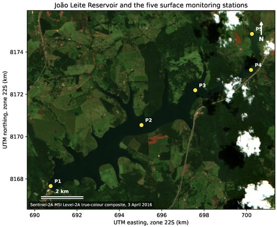
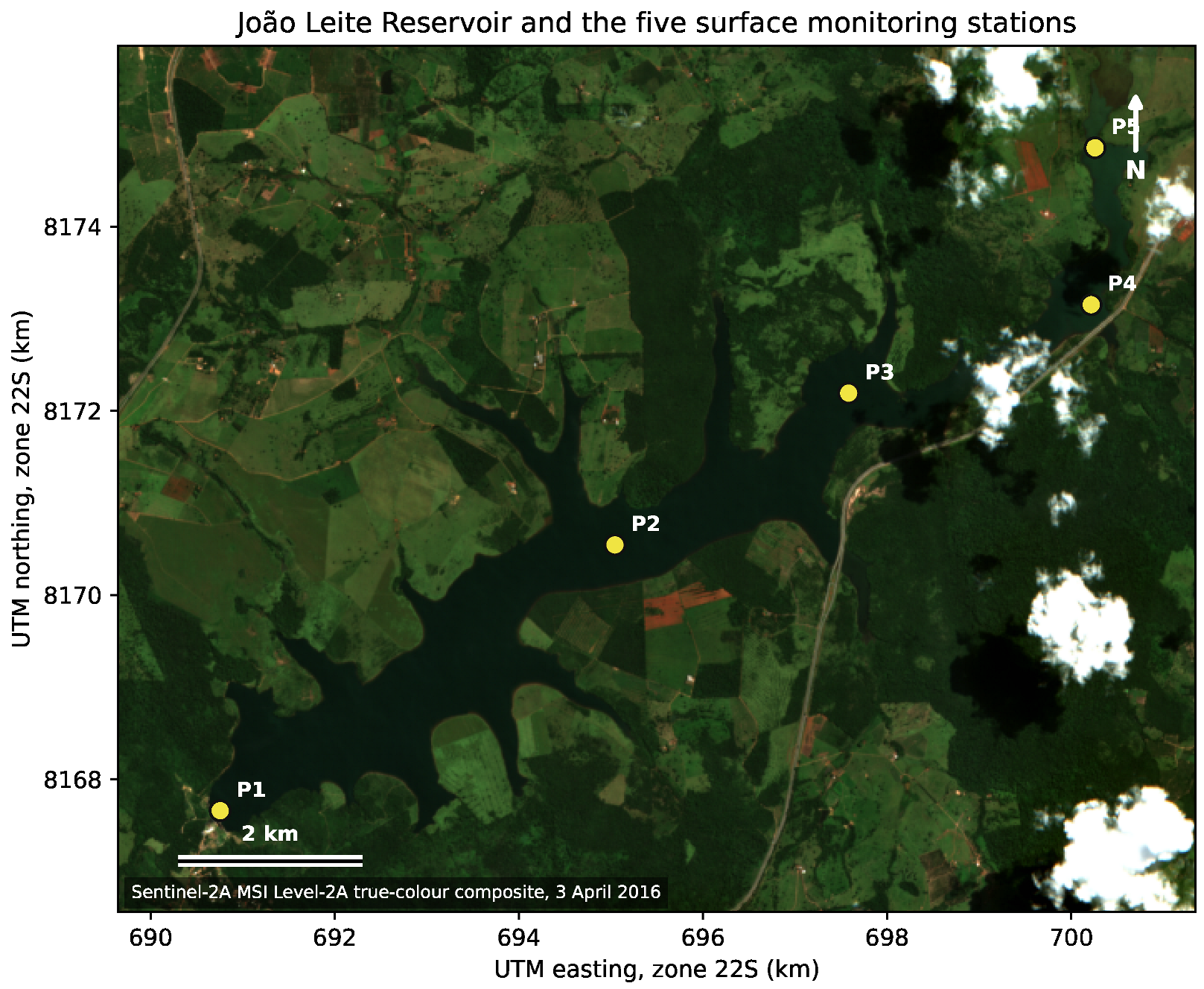
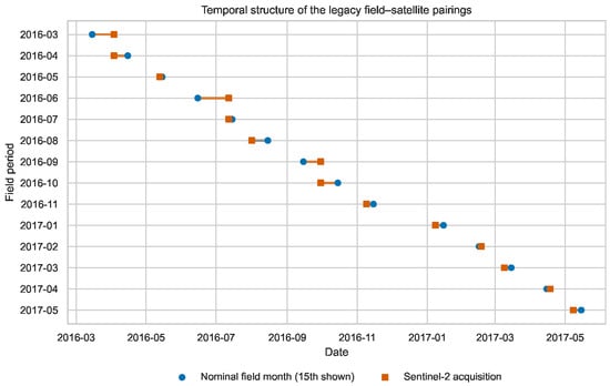
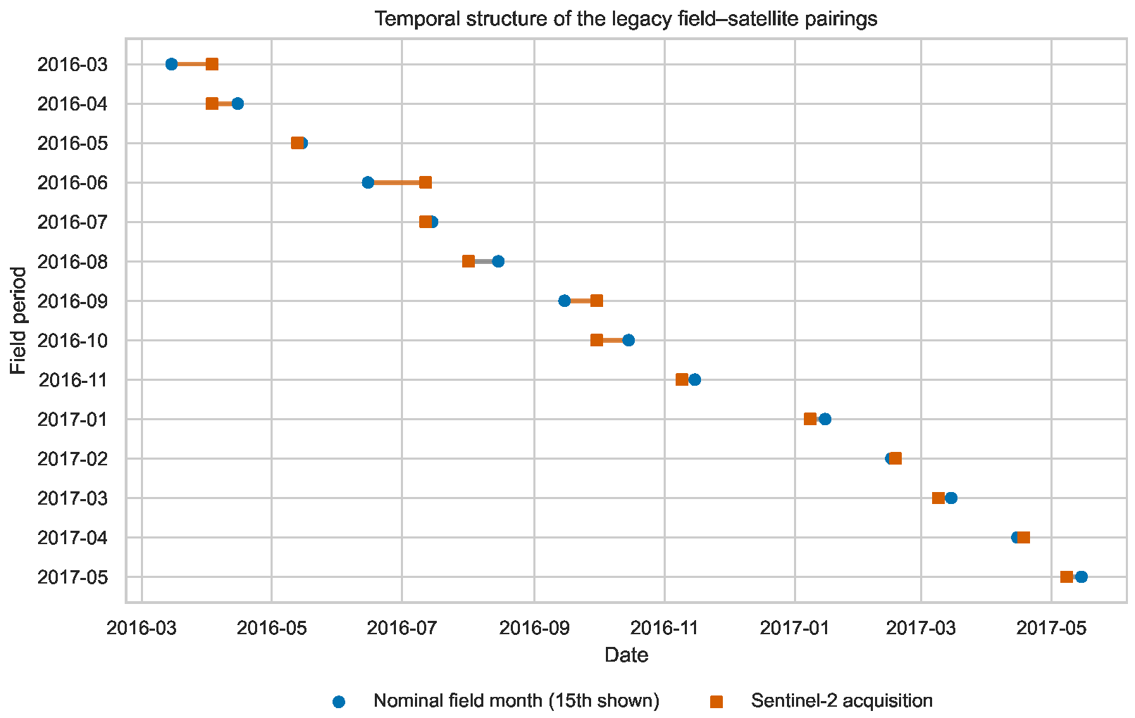
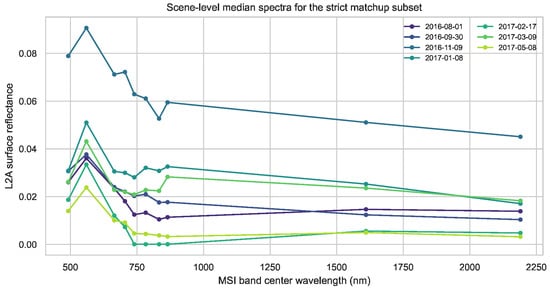
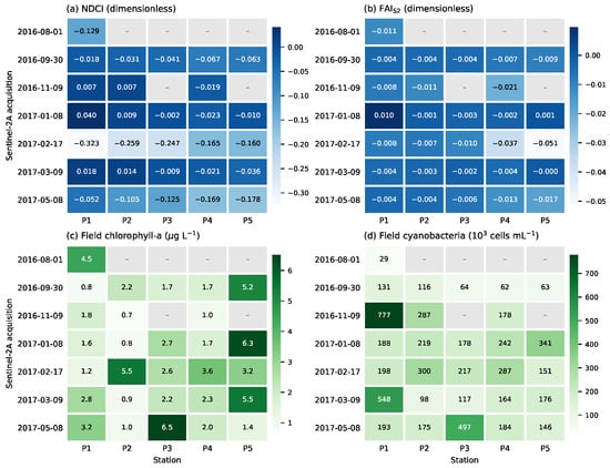
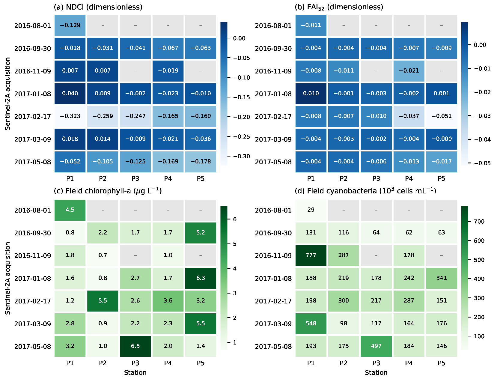
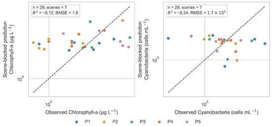
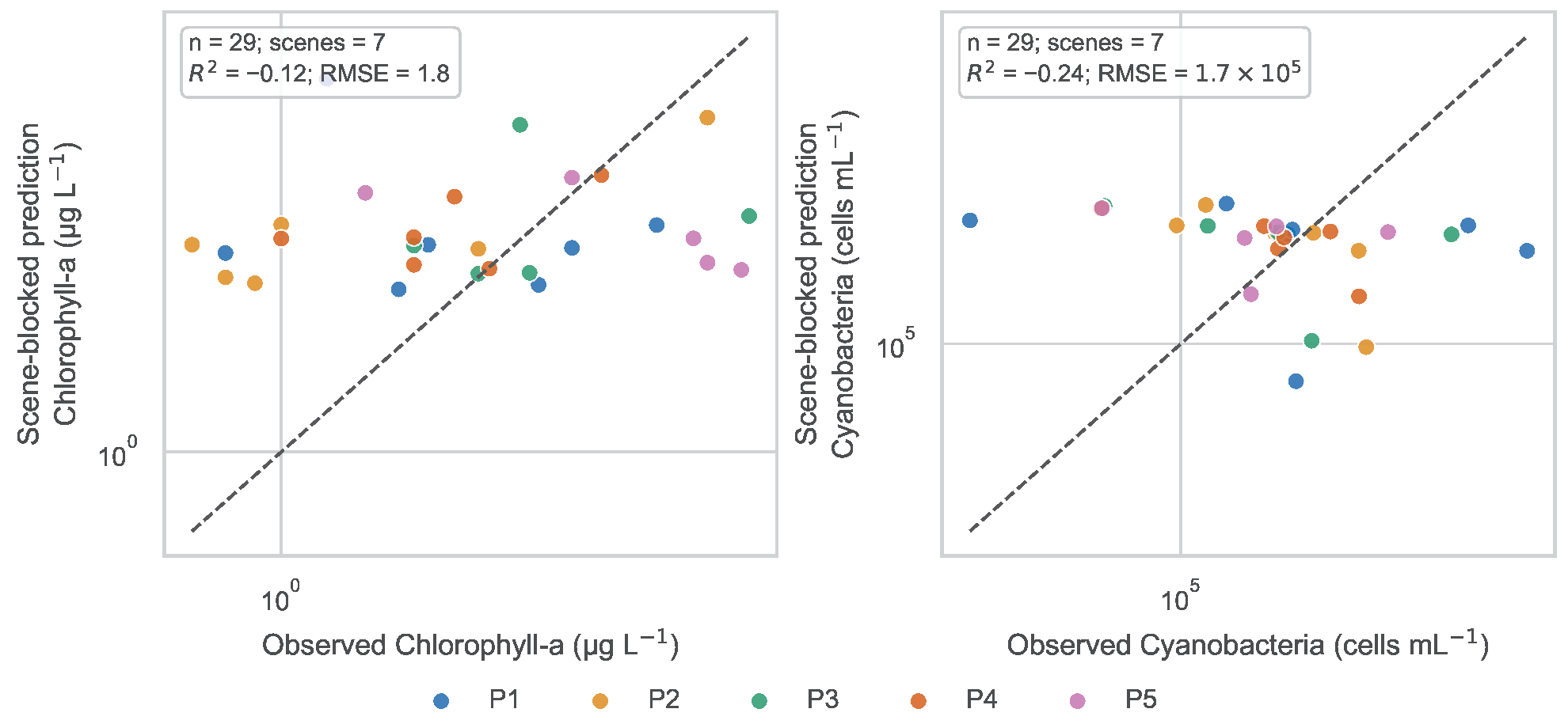

Disclaimer/Publisher’s Note: The statements, opinions and data contained in all publications are solely those of the individual author(s) and contributor(s) and not of MDPI and/or the editor(s). MDPI and/or the editor(s) disclaim responsibility for any injury to people or property resulting from any ideas, methods, instructions or products referred to in the content. |
© 2026 by the authors. Licensee MDPI, Basel, Switzerland. This article is an open access article distributed under the terms and conditions of the Creative Commons Attribution (CC BY) license.