The Regular n-Flake Dust in ℝ² Is Not Minkowski Measurable

Abstract

The Minkowski measurability of self-similar sets is closely linked to the lattice or non-lattice nature of the contraction ratios of the underlying iterated function system. A long-standing conjecture of Lapidus asserts that under certain conditions a self-similar fractal set is not Minkowski measurable if and only if it is of lattice-type. While the conjecture has been confirmed for self-similar subsets of $\mathbb{R}$, the lattice case remains open in general in higher dimensions. This paper establishes non-Minkowski measurability for a class of regular n-flake dusts in ${\mathbb{R}}^2$. The proof uses hole points to show that the parallel volume fails to be twice differentiable at a critical radius, ruling out constancy of the associated log-periodic normalized volume. These results provide further support for the Lapidus conjecture.

1. Introduction

The Minkowski content can be viewed as a tool for describing the geometry of a fractal set beyond their (Hausdorff or Minkowski) dimension, particularly for distinguishing between sets of the same dimension. This makes it a natural question to determine which sets are Minkowski measurable and to understand the mechanisms that lead to measurability or its failure.

Over the past decades, substantial progress has been made in the study of Minkowski measurability, especially in the context of self-similar sets generated by iterated function systems (IFS) satisfying the open set condition (OSC). A central theme in this area is the relationship between geometric properties of the attractor and algebraic properties of the underlying system. In this direction, Lapidus formulated a conjecture in the 1990s asserting that Minkowski measurability should be equivalent to the non-lattice property of the IFS, see [1]. This condition depends only on the logarithms of the contraction ratios and is therefore easy to verify, making it particularly appealing as a potential characterization.

The non-lattice case is by now well understood: Gatzouras [2] showed that self-similar sets in ${\mathbb{R}}^d$ satisfying the OSC are Minkowski measurable whenever the associated IFS is non-lattice. In contrast, the lattice case presents significantly greater difficulties. In dimension one, the conjecture has been completely resolved through the work of several authors, culminating in a full characterization of Minkowski measurability for self-similar subsets of $\mathbb{R}$ [3,4]. However, for dimensions $d\ge 2$, the situation remains far from settled, and a complete understanding is still lacking. We refer to [5] for a comprehensive overview of the current state of the art.

In higher dimensions, available results typically require additional structural assumptions. One prominent example is the pluriphase condition, which yields non-Minkowski measurability for certain lattice self-similar sets under suitable hypotheses [6]. This approach, as well as several related results, is based on renewal-theoretic methods and the analysis of scaling functions associated with the parallel volume. Another line of research focuses on exact tube formulas and employs techniques from the theory of complex dimensions and fractal zeta functions. While this framework has proven to be very powerful and has led to deep insights, it often involves technically demanding computations and is not always easily applicable to concrete families of sets.

The main objective of this paper is to investigate the Minkowski measurability of a class of self-similar sets in ${\mathbb{R}}^2$, namely the so-called n-flake dusts. These sets form families of lattice self-similar sets satisfying the open set condition, and thus provide a suitable testing ground for the conjectured relationship between lattice structure and non-measurability.

Our main result shows that, under a geometric condition on the contraction ratio, n-flake dusts fail to be Minkowski measurable. The proof is based on a detailed analysis of the volume of parallel sets and exploits the presence of hole points, a notion introduced in Section 2.5, which induce a lack of smoothness in the associated volume function. More precisely, we show that the function $\epsilon \mapsto {\lambda }^2\left(F_{\epsilon }\right)$ is not twice differentiable at a critical scale, which implies that the corresponding normalized volume function cannot be constant. This approach provides a new mechanism for establishing non-Minkowski measurability in the lattice case and thus contribute further evidence toward the conjectured characterization of Minkowski measurability beyond one dimension.

The paper is organized as follows. Section 2 contains the required preliminaries (see Section 2.1, Section 2.2, Section 2.3, Section 2.4 and Section 2.5) together with a brief overview of known results (see Section 2.6). In Section 3, we introduce the class of n-flake dusts and discuss their relation to the general framework. Section 4 is devoted to the proof of the main result on Minkowski non-measurability of n-flake dusts.

2. Preliminaries

The necessary terminology is established first to enable the formulation and proof of the main results. See [7] for background on fractal geometry. We follow the notation and terminology introduced in [8] and add the concept of hole points.

2.1. Minkowski Measurability

Let $({\mathbb{R}}^d,\parallel ·\parallel )$ be the d-dimensional Euclidean space and denote by

$$\mathcal{H}\left({\mathbb{R}}^d\right):=\{K\subset {\mathbb{R}}^d\mid K\ne \varnothing \mathrm{and}K\mathrm{is}\mathrm{compact}\}$$

the corresponding Hausdorff space. For $A\in \mathcal{H}\left({\mathbb{R}}^d\right)$, $\epsilon >0$ define the ε- parallel set of A as

$$A_{\epsilon }:=\{x\in {\mathbb{R}}^d\mid \mathrm{dist}(x,A)\le \epsilon \},$$

where $\mathrm{dist}(A,B):=\inf \{\parallel x-y\parallel \mid x\in A,y\in B\}$ denotes the distance of two non-empty sets $A,B\subset {\mathbb{R}}^d$ and for a point $x\in {\mathbb{R}}^d$ we write $\mathrm{dist}(x,B):=\mathrm{dist}\left(\right\{x\},B)$. Denote by ${\lambda }^d$ the d-dimensional Lebesgue measure. If the Minkowski dimension

$${\dim }_{\mathcal{M}}\left(A\right):=d-\underset{\epsilon \searrow 0}{\lim }{\displaystyle \frac{\ln {\lambda }^d\left(A_{\epsilon }\right)}{\ln \epsilon }}$$

exists, then the Minkowski content of A is defined by

$$\mathcal{M}\left(A\right):=\underset{\epsilon \searrow 0}{\lim }{\displaystyle \frac{{\lambda }^d\left(A_{\epsilon }\right)}{{\epsilon }^{d-{\dim }_{\mathcal{M}}\left(A\right)}}},$$

provided this limit also exists in $[0,\infty ]$. The set A is called $Minkowski measurable$ if $\mathcal{M}\left(A\right)$ exists and is both positive and finite.

2.2. Self-Similar Sets, Open Set Condition, and the (Non-)Lattice Case

A finite set of contractions with at least two maps is called a iterated function system (IFS). Let $S=\{S_1,\dots ,S_N\}$, with $N\ge 2$, denote an IFS consisting of contractive similarities $S_1,\dots ,S_N$ acting on ${\mathbb{R}}^d$. Such a system is called a self-similar system. A set $F\subset {\mathbb{R}}^d$ is called self-similar if

$$F={\displaystyle \bigcup _{i=1}^n}{S}_i\left(F\right)$$

for some self-similar system.

For a set A denote by $\mathcal{P}\left(A\right)$ the power set of A. Define the (set-valued) map $\mathbf{S}:\mathcal{P}\left({\mathbb{R}}^d\right)\to \mathcal{P}\left({\mathbb{R}}^d\right)$ corresponding to the self-similar system S as

$$\mathbf{S}A:={\displaystyle \bigcup _{i=1}^N}{S}_i\left(A\right).$$

(1)

It is well known ([9]) that ${\mathbf{S}|}_{\mathcal{H}\left({\mathbb{R}}^d\right)}:\mathcal{H}\left({\mathbb{R}}^d\right)\to \mathcal{H}\left({\mathbb{R}}^d\right)$ has a unique fixed point F which is called the (self-similar) attractor of the self-similar system S.

The IFS S is said to satisfy the open set condition (OSC) if there exits a non-empty bounded open set $O\subset {\mathbb{R}}^d$ such that

$${\displaystyle \bigcup _{i=1}^N}{S}_i\left(O\right)\subseteq O\mathrm{and}{S}_i\left(O\right)\cap S_j\left(O\right)=\varnothing \forall i,j=1,\dots ,N\mathrm{with}i\ne j.$$

(2)

A self-similar system that satisfies the (OSC) is called an (OSC) self-similar system. Any non-empty bounded open set O satisfying (2) is called a feasible open set for S. If S satisfies the (OSC) with feasible set O and in addition $O\cap F\ne \varnothing$ holds, then we say S satisfies the strong open set condition (SOSC) and O is called a strong feasible open set. Note that it was shown in [10] that if a self-similar system satisfies (OSC), then it possesses a strong feasible open set.

Denote the scaling ratio of $S_i$ by $r_i$, $i=1,\dots ,N$. The self-similar system S is said to be lattice if $\{\ln r_1,\dots ,\ln r_N\}$ generates a discrete subgroup of $(\mathbb{R},+).$ Otherwise, S is said to be non-lattice. If S is lattice, then there exists a largest $a>0$ such that $\{\ln r_1,\dots ,\ln r_N\}\subseteq a\mathbb{Z}$ and ${\mathrm{e}}^a$ is called the base of S.

2.3. Non-Trivial Sets and Projection Condition

Let $F\in \mathcal{H}\left({\mathbb{R}}^d\right)$ be the attractor of a (OSC) self-similar system $S=\{S_1,\dots ,S_N\}$. F is called non-trivial if there exists a feasible open set O such that

$$O⊈\overline{\mathbf{S}O},$$

(3)

where $\overline{B}$ denotes the closure of $B\subseteq {\mathbb{R}}^d$; otherwise, F is called trivial. F is non-trivial if and only if F has empty interior, which is equivalent to F having a Minkowski dimension strictly less than d, as shown in [11]. In particular, non-triviality is independent of the choice of the feasible set O.

Let ${\pi }_A$ denote the metric projection onto A for a non-empty compact set $A\in \mathcal{H}\left({\mathbb{R}}^d\right)$, which is defined for points $x\in {\mathbb{R}}^d$ that have a unique nearest point y in A by

$${\pi }_F\left(x\right):=y.$$

The set O is said to satisfy the projection condition, if

$$S_i\left(O\right)\subseteq \overline{{\pi }_F^{-1}\left(S_{i}F\right)}$$

for all $i=1,\dots ,N$. It is worth noting that, as long as (OSC) holds, it is always possible to find a strong feasible open set that satisfies the projection condition (see [12]).

2.4. Pluriphase Condition

For a given self-similar system S with non-trivial attractor $F\in \mathcal{H}\left({\mathbb{R}}^d\right)$ and a fixed feasible open set O, define

$$\Gamma :={\Gamma }_O:=O\setminus \mathbf{S}O$$

and

$$g:=\underset{x\in \Gamma }{\sup }\{\underset{y\in F}{\min }\{\parallel x-y\parallel \left\}\right\}.$$

The set F is said to be pluriphase with respect to ${\Gamma }_O$ if there exists a finite partition $0=:a_0<a_1<\dots <a_M:=g<\infty$ of the interval $(0,\infty )$ and constants ${\kappa }_{m,k}\in \mathbb{R},m=1,\dots ,M,k=0,\dots ,d$, such that for all $\epsilon >0$

$${\lambda }^d(F_{\epsilon }\cap \Gamma )={\displaystyle \sum _{m=1}^M}{\mathbb{1}}_{(a_{m-1},a_m]}\left(\epsilon \right){\displaystyle \sum _{k=0}^d}{\kappa }_{m,k}{\epsilon }^{d-k}+{\mathbb{1}}_{(g,\infty )}\left(\epsilon \right){\lambda }^d(\Gamma ).$$

(4)

Here ${\mathbb{1}}_A$ denotes the indicator function of a set A.

2.5. Hole Points

For a set $A\in \mathcal{H}\left({\mathbb{R}}^d\right)$ we introduce our concept of hole points as a special case of the well-known concept of critical points of the distance function $d_A\left(x\right):=\mathrm{dist}(x,A)$.

For $A\subseteq {\mathbb{R}}^d$, let $\mathrm{conv}\left(A\right)$ and $\mathrm{int}\left(A\right)$ denote the convex hull and the interior of A, respectively.

Definition 1.

Let $A\in \mathcal{H}\left({\mathbb{R}}^d\right)$. The point $x\in {\mathbb{R}}^d\setminus A$ is called a critical point if $x\in \mathrm{conv}\left({\Sigma }_A\left(x\right)\right)$, where ${\Sigma }_A\left(x\right):=\{a\in A:\parallel a-x\parallel =d(x,A)\}$.

Remark 1.

Let $f:{\mathbb{R}}^d\to \mathbb{R}$ be a locally Lipschitz function. For $x\in {\mathbb{R}}^d$ denote ${\partial }^{\circ }f\left(x\right)$ the Clarke generalized gradient of f at x (also called the Clarke subdifferential). Suppose that $p\in {\mathbb{R}}^d$ has $0\in {\partial }^{\circ }f\left(p\right)$, then p is called critical point of f (cf. [13], Chap. 2, and [14]).

According to a result by Fu ([15], Lemma 4.2), for any $A\in \mathcal{H}\left({\mathbb{R}}^d\right)$, a point $x\in {\mathbb{R}}^d\setminus A$ is a critical point of the distance function $d_A$ (in the sense of Clarke) if and only if x is a critical point.

Definition 2.

Let $A\in \mathcal{H}\left({\mathbb{R}}^d\right)$. A point $x\in {\mathbb{R}}^d$ is called hole point of A if $x\in \mathrm{int}\left(\mathrm{conv}\left({\Sigma }_A\left(x\right)\right)\right)$. Denote by $\mathrm{Hp}\left(A\right)$ the set of all hole points of A. The set $\mathrm{Hv}\left(A\right):=\left\{d\right(x,A):x\in \mathrm{Hp}(A\left)\right\}$ denotes the set of hole values.

Definition 3.

Let $A\in \mathcal{H}\left({\mathbb{R}}^d\right)$ and let $\epsilon >0$. A set $H\subset {\mathbb{R}}^d$ is called a hole of $A_{\epsilon }$ if H is a bounded connected component of ${\mathbb{R}}^d\setminus A_{\epsilon }$.

Lemma 1.

Let $A\in \mathcal{H}\left({\mathbb{R}}^d\right)$. Then every $x\in \mathrm{Hp}\left(A\right)$ lies in a hole of $A_{\epsilon }$ for some $\epsilon >0$.

Proof. 

Let $x\in \mathrm{Hp}\left(A\right)$ and $v_x:=d(x,A)$. By definition of ${\Sigma }_A\left(x\right)$, for all $a\in {\Sigma }_A\left(x\right)$, $\parallel a-x\parallel =v_x$. By Caratheodory’s Theorem, there exists a finite subset $S=\{a_0,\dots ,a_k\}\subseteq {\Sigma }_A\left(x\right)$ (with $k\le d$) such that $x\in \mathrm{int}\left(\mathrm{conv}\right(S\left)\right)$. Let $P:=\mathrm{conv}\left(S\right)$ be this simplex.

For each $(d-1)$-dimensional (maximal) facet $\mathsf{\Phi }\subset \partial P$, let $h_{\mathsf{\Phi }}$ be the distance from x to (the affine hull of) $\mathsf{\Phi }$. Since $x\in \mathrm{int}\left(P\right)$, we have $h_{\mathsf{\Phi }}>0$ for all facets. The circumradius $R_{\mathsf{\Phi }}$ of each facet $\mathsf{\Phi }$ is given by $R_{\mathsf{\Phi }}=\sqrt{v_x^2-h_{\mathsf{\Phi }}^2}<v_x$.

Let $R_{max}={\max }_{\mathsf{\Phi }}{R}_{\mathsf{\Phi }}$. Choose $\epsilon$ such that $R_{max}<\epsilon <v_x$. First, since $\epsilon <v_x=d(x,A)$, it holds that $x\notin A_{\epsilon }$. Second, consider any path $\gamma \left(t\right)=x+tv$ for a unit vector $v\in {\mathbb{R}}^d$. Since $x\in \mathrm{int}\left(P\right)$, every ray must intersect some facet $\mathsf{\Phi }$ of $\partial P$ at a point p. The distance from p to the nearest vertex $a_i$ of $\mathsf{\Phi }$ is at most $R_{\mathsf{\Phi }}\le R_{max}<\epsilon$. Thus, $p\in B(a_i,\epsilon )\subseteq A_{\epsilon }$.

Because every path from x to infinity must cross $\partial P\subset A_{\epsilon }$, x is contained in a bounded connected component of ${\mathbb{R}}^d\setminus A_{\epsilon }$. □

Lemma 2.

Let $F\in \mathcal{H}\left({\mathbb{R}}^d\right)$. Then $\mathrm{Hp}\left(F\right)\subseteq \mathrm{conv}\left(F\right)\setminus F.$

Proof. 

Let $x\in F$. Then $d(x,F)=0$ and hence ${\Sigma }_F\left(x\right)=\left\{x\right\}.$ Therefore $\mathrm{int}\left(\mathrm{conv}\left({\Sigma }_F\left(x\right)\right)\right)=\varnothing$ so $x\notin \mathrm{Hp}\left(F\right)$.

Now let $x\notin \mathrm{conv}\left(F\right)$. Since ${\Sigma }_F\left(x\right)\subseteq F,$ we have $\mathrm{conv}\left({\Sigma }_F\left(x\right)\right)\subseteq \mathrm{conv}\left(F\right).$ Thus $x\notin \mathrm{conv}\left({\Sigma }_F\left(x\right)\right)$ and, in particular, $x\notin \mathrm{int}\left(\mathrm{conv}\left({\Sigma }_F\left(x\right)\right)\right).$ Hence $x\notin \mathrm{Hp}\left(F\right)$. □

Remark 2.

The hole points and hole values are determined explicitly in the following two classical examples, using their standard IFSs.

1. 

Let $C\subset [0,1]$ be the middle-third Cantor set. By Lemma 2, every hole point lies in a connected component $(a,b)$ of $[0,1]\setminus C$. For $x\in (a,b)$,

$${\Sigma }_C\left(x\right)=\left\{\begin{array}{cc}\left\{a\right\},\hfill & x<{\displaystyle \frac{a+b}{2}},\hfill \\ \{a,b\},\hfill & x={\displaystyle \frac{a+b}{2}},\hfill \\ \left\{b\right\},\hfill & x>{\displaystyle \frac{a+b}{2}}.\hfill \end{array}\right.$$

Hence the unique hole point in $(a,b)$ is its midpoint. Therefore

$$\mathrm{Hp}\left(C\right)={\displaystyle \bigcup _{n=0}^{\infty }}{\mathbf{S}}^n\left\{{\displaystyle \frac{1}{2}}\right\}.$$

Since the complementary intervals have lengths $3^{-n}$,

$$\mathrm{Hv}\left(C\right)=\left\{{\displaystyle \frac{1}{2·3^n}}:n\in \mathbb{N}\right\}.$$

2. 

Let $F\subset {\mathbb{R}}^2$ be the classical Sierpinski triangle and let $T:=\mathrm{conv}\left(F\right)$. By Lemma 2, every hole point lies in a connected component H of $T\setminus F$. Since H is an equilateral triangle and $\partial H\subset F$, one has ${\Sigma }_F\left(x\right)={\Sigma }_{\partial H}\left(x\right)$ for all $x\in H.$ Denote by $c_H$ the center of $H.$ For $x\in H$ with $x\ne c_H$, at most two sides of $\partial H$ are nearest to x, and hence $\mathrm{int}\left(\mathrm{conv}\left({\Sigma }_F\left(x\right)\right)\right)=\varnothing$ and $x\notin \mathrm{Hp}\left(F\right).$

For $c_H$, the set ${\Sigma }_F\left(c_H\right)$ consists of the three orthogonal projections $p_1,p_2,p_3$ of $c_H$ onto the three sides of H. Then ${\Sigma }_F\left(c_H\right)=\{p_1,p_2,p_3\}$ and $c_H={\displaystyle \frac{1}{3}}(p_1+p_2+p_3).$ Since $p_1,p_2,p_3$ are not collinear, it follows that $c_H\in \mathrm{int}\left(\mathrm{conv}\left({\Sigma }_F\left(c_H\right)\right)\right),$ and hence $c_H\in \mathrm{Hp}\left(F\right)$. Consequently, denoting the centre of T by $c_T$, one obtains

$$\mathrm{Hp}\left(F\right)={\displaystyle \bigcup _{n=0}^{\infty }}{\mathbf{S}}^n\left\{c_T\right\}.$$

If g denotes the hole value corresponding to the first removed triangle, self-similarity yields

$$\mathrm{Hv}\left(F\right)=\left\{2^{-n}g:n\in {\mathbb{N}}_0\right\}.$$

Remark 3.

The sets $\mathrm{Hp}\left(A\right)$ and $\mathrm{Hv}\left(A\right)$ are not necessarily closed. For example, as seen in the preceding remark, for the middle-third Cantor set C, it is easy to see that $\mathrm{Hp}\left(C\right)$ and $\mathrm{Hv}\left(C\right)$ are not closed.

2.6. Known Results on Minkowski Measurability of Self-Similar Sets

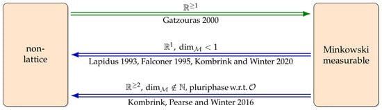
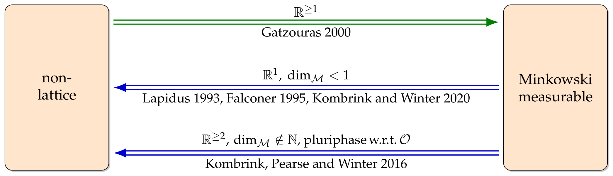
The principal results on Minkowski measurability for self-similar sets in ${\mathbb{R}}^d$ are reviewed in order to clarify its relationship with the non-lattice property. A schematic illustration is provided in Figure 1.

Figure 1. Overview of the relationships between non-lattice and Minkowski measurability of self-similar sets satisfying the (OSC), see Figure 1 in [8].

Theorem 1

(Gatzouras [2]). Let $F\in \mathcal{H}\left({\mathbb{R}}^d\right)$ be the attractor of a non-lattice (OSC) self-similar system. Then F is Minkowski measurable.

Theorem 2

(Falconer [3] and Kombrink, Winter [4]). Let $F\in \mathcal{H}\left(\mathbb{R}\right)$ be the attractor of a lattice (OSC) self-similar system with ${\dim }_{\mathcal{M}}F<1$. Then F is not Minkowski measurable.

Taken together, Theorems 1 and 2 provide a full characterization of Minkowski measurability for self-similar sets in $\mathbb{R}$ generated by an (OSC) IFS S. If the Minkowski dimension is below 1, Minkowski measurability holds if and only if S satisfies the non-lattice condition. It is currently unknown whether this characterization extends to higher-dimensional settings. A partial step toward this question is given in Theorem 3.

Theorem 3

(Kombrink, Pearse, Winter, [6]). Let $F\in \mathcal{H}\left({\mathbb{R}}^d\right)$ be the attractor of an lattice (OSC) self-similar system with ${\dim }_{\mathcal{M}}F\notin \mathbb{N}$. Suppose that there exists a strong feasible open set O satisfying the projection condition such that F is pluriphase with respect to ${\Gamma }_O$. Then F is not Minkowski measurable.

Remark 4.

Note that it is essential to exclude sets with an integer Minkowski dimension from the Lapidus conjecture. This limitation can be illustrated by a continuous family of one-dimensional counterexamples. For any parameter $r\in (0,1)$, consider the self-similar system $S^{\left(r\right)}$ on $\mathbb{R}$ defined by

$$S_1^{\left(r\right)}\left(x\right)=rx,S_2^{\left(r\right)}\left(x\right)=(1-r)x+r.$$

The attractor is invariably the unit interval $F=[0,1]$ and trivially Minkowski measurable (and pluriphase) for all r. However, the system is lattice if and only if $\log \left(r\right)/\log (1-r)\in \mathbb{Q}$ (e.g., when $r=1/2$). For all other choices (e.g., $r=1/3$), the system is non-lattice. Similarly, a simple two-dimensional counterexample is given by the (OSC) self-similar system S on ${\mathbb{R}}^2$ defined by

$$S_1\left(x\right)=\frac{1}{2}x,S_2\left(x\right)=\frac{1}{2}x+(\frac{1}{2},0),S_3\left(x\right)=\frac{1}{2}x+(0,\frac{1}{2}),S_4\left(x\right)=\frac{1}{2}x+(\frac{1}{2},\frac{1}{2}).$$

The attractor of S is the unit square $F={[0,1]}^2$. Clearly, F is Minkowski measurable (and pluriphase), but the underlying IFS S is lattice.

3. n-Flake Dusts

Let $n\in \mathbb{N}$ with $n\ge 3$ and $r\in (0,1)$. For a regular n-gon with vertices $V_1,\dots ,V_n\in {\mathbb{R}}^2$, an IFS is given by the set of n contractive similarity mappings $\mathcal{S}:={\mathcal{S}}^{n,r}:=\{{\mathcal{S}}_1,\dots ,{\mathcal{S}}_n\}$:

$${\mathcal{S}}_i\left(x\right):=rx+(1-r)V_i,\mathrm{for}i=1,\dots ,n.$$

Note, the contraction ratio r required for the sub-polygons to just touch is:

$$r={\displaystyle \frac{1}{2}}{\left({\displaystyle 1+\sum _{k=1}^{\lfloor n/4\rfloor }\cos \frac{2\pi k}{n}}\right)}^{-1}=:R_n,$$

(5)

see for example [16]. The attractor of $\mathcal{S}$ is called n-flake or Sierpinski n-gon. If $r<R_n$, then the attractor of $\mathcal{S}$ is specified as n-flake dust and denoted by $\mathcal{F}:={\mathcal{F}}^{n,r}$.

Since $r<R_n$, the IFS $\mathcal{S}$ satisfies (OSC), with the feasible open set

$$\mathcal{O}:={\mathcal{O}}_n:=\mathrm{int}\left(\mathrm{conv}\left(\{V_1,\dots ,V_n\}\right)\right).$$

Indeed, even the strong separation condition, i.e., $S_i\left(\mathcal{F}\right)\cap S_j\left(\mathcal{F}\right)=\varnothing$ for all $i\ne j$ holds. Therefore, by the Hutchinson dimension formula [9], ${\mathcal{F}}^{n,r}$ has Minkowski (and Hausdorff) dimension

$$D:=D^{n,r}:={\dim }_{\mathcal{M}}\left(\mathcal{F}\right)=-{\displaystyle \frac{\ln n}{\ln r}}\in (0,2).$$

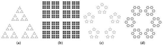
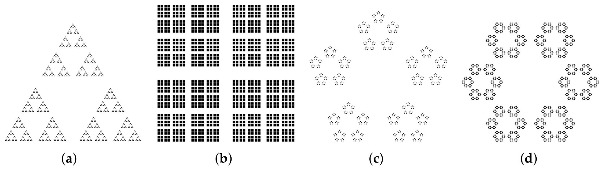
Thus ${\mathcal{F}}^{n,r}$ is non-trivial for all $n\ge 3$ and all $r\in (0,R_n)$. Further, ${\mathcal{F}}^{n,r}$ is lattice with base r for all $n\ge 3$ and all $r\in (0,R_n)$; see Figure 2 for some examples.

Figure 2. Visualization of the families ${\mathcal{F}}^{n,r}$ for various values of n and r. (a) $n=3,r=0.45$. (b) $n=4,r=0.45$. (c) $n=5,r=0.3$. (d) $n=6,r=0.3$.

Remark 5.

For $n=4$ and $r<R_4=1/2$ we have ${\mathcal{F}}^{n,r}=C^{1/r}$ the Cantor dust set discussed in [8]. Therein, it is shown that ${\mathcal{F}}^{4,r}$ is not Minkowski measurable for $r<1/30.$ For $1/2>r>1/30$ it is only conjectured that $C^{1/r}$ is not Minkowski measurable. In [8] it is further shown that, for all $r\in (0,1/2)$${\mathcal{F}}^{4,r}$ is not pluriphase with respect to ${\Gamma }_{\mathcal{O}}$ for the IFS ${\mathcal{S}}^{4,r}$ and the feasible set $\mathcal{O}={\mathcal{O}}_4$. Consequently, Theorem 3 is not readily applicable to prove that ${\mathcal{F}}^{n,r}$ is not Minkowski measurable.

4. Main Result

In this section we study the Minkowski measurability of the sets $\mathcal{F}={\mathcal{F}}^{n,r}$ for any $n\in \mathbb{N}$. The main result is stated in Theorem 5: for each $n\ge 3$, a family of n-flake dusts $\mathcal{F}$ is not Minkowski measurable.

Let $a>0$. A function $h:(0,\infty )\to \mathbb{R}$ is said to be log-periodic on $(0,a]$ with scaling factor $\rho \in (0,1)$, if it satisfies the equation

$$h\left(\rho x\right)=h\left(x\right)\forall x\in (0,a].$$

For $\mathcal{F}$ consider the function $f:(0,\infty )\to [0,\infty )$

$$f\left(\epsilon \right):={\displaystyle \frac{{\lambda }^2\left({\mathcal{F}}_{\epsilon }\right)}{{\epsilon }^{2-D}}}.$$

If f is log-periodic on $(0,a]$ for $a>0$, then $\mathcal{F}$ is Minkowski measurable if and only if f is constant. Thus, to show that $\mathcal{F}$ is not Minkowski measurable it suffices to prove that

(1)

f is log-periodic for sufficiently small $\epsilon$

(2)

f is not constant.

For the latter, it is enough to show that f is not $C^2$ at some point ${\epsilon }_0<a$. By the following Lemma 3, this reduces to showing that the function $\epsilon \mapsto {\lambda }^2\left({\mathcal{F}}_{\epsilon }\right)$ is not $C^2$ at ${\epsilon }_0$, where $C^k$ ($k\in \mathbb{N}$) denotes the k-times continuously differentiable functions.

Lemma 3.

Let u be a $C^k$ function that is not $C^{k+1}$ for some $k\in \mathbb{N}$, and let v be a $C^{k+1}$ function that is nowhere zero. Then their quotient $u/v$ cannot be constant.

Proof. 

Suppose that the quotient is constant, meaning $u/v=c$ for some constant $c\in \mathbb{R}$. This implies that $u=c·v$. Since $v\in C^{k+1}$ it follows that $u\in C^{k+1}$. This directly contradicts the assumption that u is not $C^{k+1}$. □

To prove that the function $\epsilon \mapsto {\lambda }^2\left(F_{\epsilon }\right)$ is not $C^2$ we recall the following well-known result:

Theorem 4

(([17] Corollary 2.5), based on [18,19]). Let $A\in \mathcal{H}\left({\mathbb{R}}^d\right)$ and $\epsilon \mapsto V_A\left(\epsilon \right):={\lambda }^d\left(A_{\epsilon }\right)$ differentiable in ${\epsilon }_0$. Then $V_A^{\prime }\left({\epsilon }_0\right)={\mathcal{H}}^{d-1}(\partial A_{{\epsilon }_0})$.

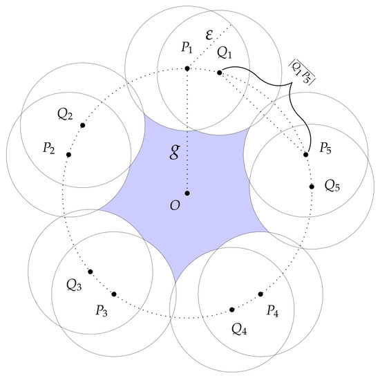
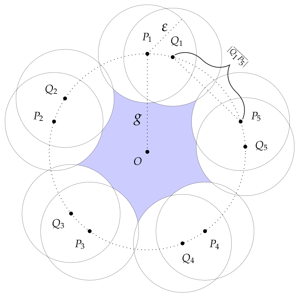
Intuitively, the key observation is that the function $\epsilon \mapsto {\lambda }^2\left({\mathcal{F}}_{\epsilon }\right)$ is no longer ${\mathcal{C}}^2$ at the value ${\epsilon }_0:=\sup \{\epsilon >0:{\mathcal{F}}_{\epsilon }\mathrm{has}\mathrm{a}\mathrm{hole}\}$. Figure 3 illustrates the appearance of this “first hole” depending on n, r and $\epsilon$.

Figure 3. Illustration of the set ${\mathbb{B}}_{n,g,\theta }\left(\epsilon \right)$ (marked in blue) for $n=5$ and $\theta =\pi /12$.

Next, we develop a lemma showing that the area of the “first hole” is not $C^2$, which is a crucial reason why the map $\epsilon \mapsto {\lambda }^2\left({\mathcal{F}}_{\epsilon }\right)$ is not $C^2$.

Let $\mathtt{g}>0$. Let $P_i\in {\mathbb{R}}^2,$$i=1,\dots ,n$ the vertices of a regular n-gon with outer radius $\mathtt{g}$. Denote its centroid by O. Let $\theta \in [0,{\displaystyle \frac{\pi }{n}})$ and denote $Q_i\in {\mathbb{R}}^2,$$i=1,\dots ,n$ the vertices of the n-gon rotated counter-clockwise by $\theta$, see Figure 3. Let $\epsilon >{\displaystyle \frac{1}{2}}\left|\overline{Q_1{P}_n}\right|$, where $\overline{PQ}:=\mathrm{conv}\{P,Q\}$ denotes the line segment between $P,Q\in {\mathbb{R}}^2$ with length $|\overline{PQ}|:=\mathrm{dist}(P,Q)$. For $p\in {\mathbb{R}}^2$ and $\delta \in \mathbb{R}$ denote by $B(p,\delta ):=\{x\in {\mathbb{R}}^2\mid \parallel x-p\parallel \le \delta \}$ the disc with center p and radius $\delta .$ Denote by

$$\mathbb{B}\left(\epsilon \right):={\mathbb{B}}_{n,g,\theta }\left(\epsilon \right):=B(O,\mathtt{g})\setminus {\displaystyle \bigcup _{i=1}^n}\left(B(P_i,\epsilon )\cup B(Q_i,\epsilon )\right)$$

the blue set marked in Figure 3. Observe that ${\mathcal{F}}_{\epsilon }$ depends only on n, r and $\epsilon$. The fixed parameters g and $\theta$ are introduced to facilitate the investigation of the area of $\mathbb{B}$ as a function of $\epsilon$.

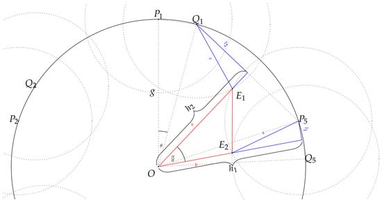
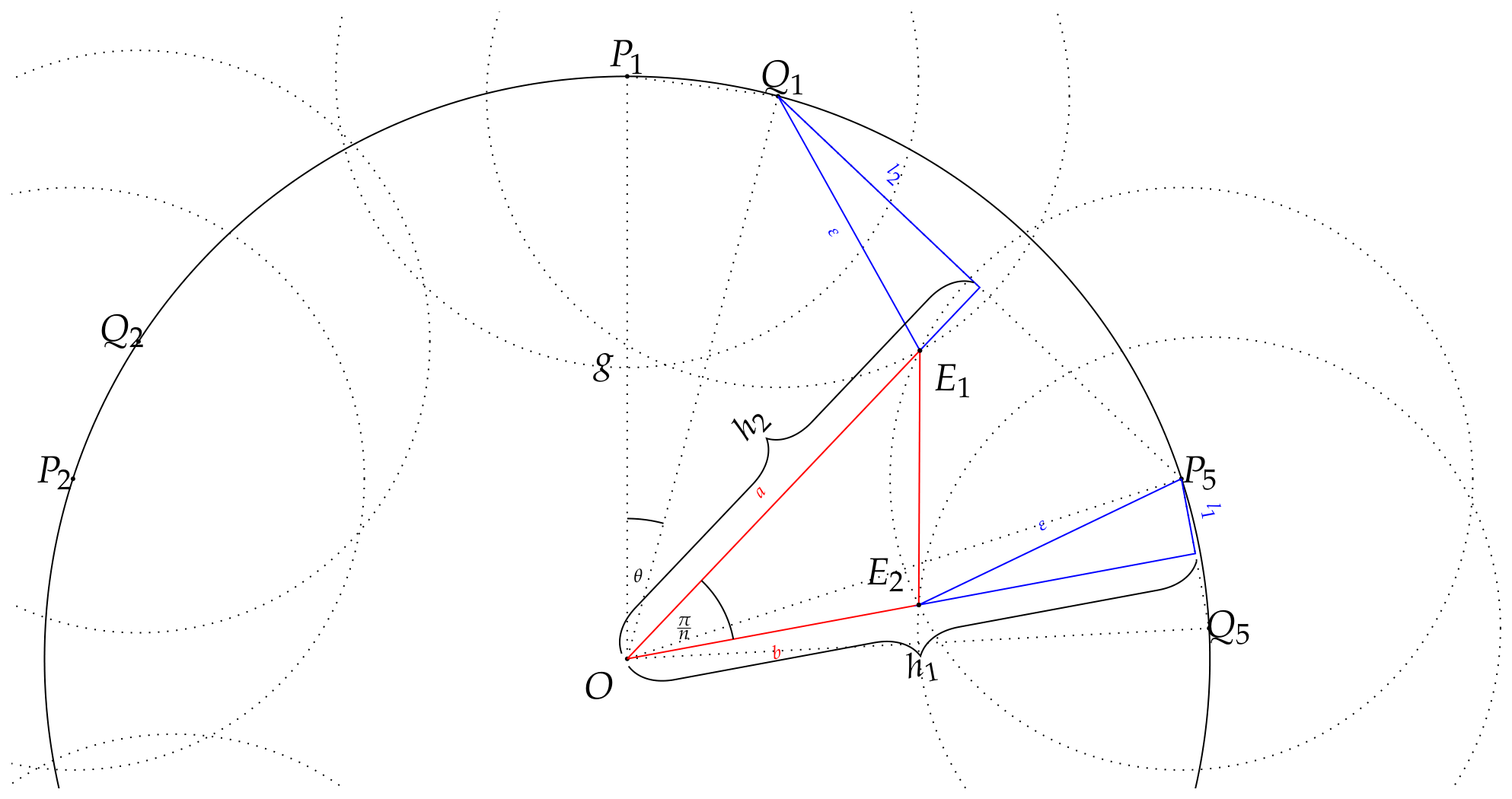
For a set $A\subset {\mathbb{R}}^2$, let $\partial A$ denote its boundary. Furthermore, we define the points $E_1$ and $E_2$ via the intersections:

$$\begin{array}{cc}\hfill \left\{E_1\right\}& :=\partial B(Q_1,\epsilon )\cap \partial B(P_n,\epsilon )\cap B(O,\mathtt{g}),\hfill \\ \hfill \left\{E_2\right\}& :=\partial B(Q_n,\epsilon )\cap \partial B(P_n,\epsilon )\cap B(O,\mathtt{g}).\hfill \end{array}$$

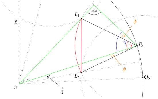
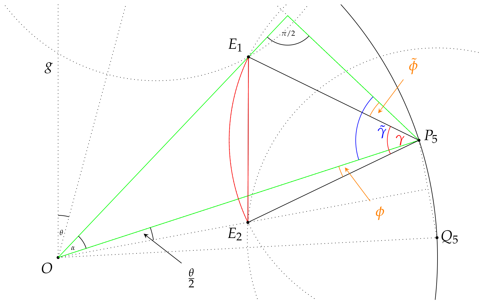
Let $A_T\left(\epsilon \right)$ be the area of the triangle $E_1{E}_{2}O$ (see Figure 4) and let $A_S\left(\epsilon \right)$ be the area of the circular segment of $B(P_n,\epsilon )$ with secant $\overline{E_1{E}_2}$, determined by radius $\epsilon$ and angle $\gamma \left(\epsilon \right):=\angle E_1{P}_n{E}_2$ (see Figure 5). The area of $\mathbb{B}$ as a function of $\epsilon$ is then given by:

$$H\left(\epsilon \right):={\lambda }^2\left(\mathbb{B}\left(\epsilon \right)\right)=\left\{\begin{array}{cc}2n[A_T\left(\epsilon \right)-A_S\left(\epsilon \right)],\hfill & {\displaystyle \frac{1}{2}}\left|\overline{Q_1{P}_n}\right|<\epsilon <\mathtt{g}\hfill \\ 0\hfill & \epsilon \ge \mathtt{g}.\hfill \end{array}\right.$$

Figure 4. Schematic setup for the calculation of $A_T\left(\epsilon \right)$.

Figure 5. Schematic setup for the calculation of $A_S\left(\epsilon \right)$.

Note that, in the proof of Theorem 5, Steps 2–4 establish that the “first hole” of ${\mathcal{F}}_{\epsilon }$ corresponds to ${\mathbb{B}}_{n,g,\theta }$ for a specific range of $\epsilon$ and fixed parameters n, g and $\theta$.

Lemma 4.

The second left derivative of $H\left(\epsilon \right)$ at $\epsilon =\mathtt{g}$ is non-zero.

Proof. 

Let $n\in \mathbb{N}$, $n\ge 3$, $\theta \in [0,{\displaystyle \frac{\pi }{n}})$. As depicted in Figure 4, denote

$$l_1:={\displaystyle \frac{1}{2}}|\overline{P_n{Q}_n}|=\mathtt{g}\sin \left({\displaystyle \frac{\theta }{2}}\right)\mathrm{and}{l}_2:={\displaystyle \frac{1}{2}}\left|\overline{Q_1{P}_n}\right|=\mathtt{g}\sin \left({\displaystyle \frac{\pi }{n}}-{\displaystyle \frac{\theta }{2}}\right),$$

and further

$$h_1:=\mathrm{dist}(O,\overline{P_n{Q}_n})=\mathtt{g}\cos \left({\displaystyle \frac{\theta }{2}}\right)\mathrm{and}{h}_2:=\mathrm{dist}(O,\overline{Q_1{P}_n})=\mathtt{g}\cos \left({\displaystyle \frac{\pi }{n}}-{\displaystyle \frac{\theta }{2}}\right).$$

Let $\epsilon \in [l_2,\infty ).$ Then the area of the red triangle in Figure 4 is

$$A_T\left(\epsilon \right)={\displaystyle \frac{a\left(\epsilon \right)·b\left(\epsilon \right)·\sin \left(\frac{\pi }{n}\right)}{2}},$$

where $a\left(\epsilon \right)$ and $b\left(\epsilon \right)$ are given by

$$a\left(\epsilon \right)=h_2-\sqrt{{\epsilon }^2-l_2^2}=\mathtt{g}\cos \left({\displaystyle \frac{\pi }{n}}-{\displaystyle \frac{\theta }{2}}\right)-\sqrt{{\epsilon }^2-g^2{\sin }^2\left({\displaystyle \frac{\pi }{n}}-{\displaystyle \frac{\theta }{2}}\right)}$$

$$b\left(\epsilon \right)=h_1-\sqrt{{\epsilon }^2-l_1^2}=\mathtt{g}\cos \left({\displaystyle \frac{\theta }{2}}\right)-\sqrt{{\epsilon }^2-{\mathtt{g}}^2{\sin }^2\left({\displaystyle \frac{\theta }{2}}\right)}.$$

The area of the circular segment (red in Figure 5) is in the notation of Figure 5 given by

$$A_S\left(\epsilon \right)={\displaystyle \frac{{\epsilon }^2}{2}}·[\gamma \left(\epsilon \right)-\sin \left(\gamma \left(\epsilon \right)\right)].$$

where the angle $\gamma \left(\epsilon \right)$ is determined by

$$\gamma \left(\epsilon \right)=\tilde{\gamma }-\tilde{\varphi }\left(\epsilon \right)+\varphi \left(\epsilon \right),$$

with

$$\tilde{\gamma }={\displaystyle \frac{\pi }{2}}-\alpha ={\displaystyle \frac{\pi }{2}}-{\displaystyle \frac{\pi }{n}}+{\displaystyle \frac{\theta }{2}}$$

and

$$\tilde{\varphi }\left(\epsilon \right)=\arccos \left({\displaystyle \frac{l_2}{\epsilon }}\right).$$

By the law of sines it is

$${\displaystyle \frac{\epsilon }{\sin (\theta /2)}}={\displaystyle \frac{b\left(\epsilon \right)}{\sin \left(\varphi \right(\epsilon \left)\right)}}$$

and therefore

$$\varphi \left(\epsilon \right)=\arcsin \left({\displaystyle \frac{b\left(\epsilon \right)}{\epsilon }}\sin \left({\displaystyle \frac{\theta }{2}}\right)\right).$$

Calculate the second left derivative of $A_T\left(\epsilon \right)={\displaystyle \frac{1}{2}}·a\left(\epsilon \right)·b\left(\epsilon \right)·\sin \left({\displaystyle \frac{\pi }{n}}\right)$ in $\mathtt{g}$:

On $(l_2,\infty )$ it is:

$$A_T^{″}={\displaystyle \frac{1}{2}}\sin \left({\displaystyle \frac{\pi }{n}}\right)\left(a^{″}b+2a^{\prime }{b}^{\prime }+a{b}^{″}\right).$$

At $\epsilon =\mathtt{g}$, since $a\left(\mathtt{g}\right)=b\left(\mathtt{g}\right)=0$ and $a^{″}$, $b^{″}$ are locally bounded at $\epsilon =\mathtt{g}$,

$$A_T^{″}\left(\mathtt{g}\right)=\sin \left({\displaystyle \frac{\pi }{n}}\right)a^{\prime }\left(\mathtt{g}\right)b^{\prime }\left(\mathtt{g}\right).$$

Using

$$a^{\prime }\left(\mathtt{g}\right)=-\sec \left({\displaystyle \frac{\pi }{n}}-{\displaystyle \frac{\theta }{2}}\right),b^{\prime }\left(\mathtt{g}\right)=-\sec {\displaystyle \frac{\theta }{2}},$$

we obtain

$$A_T^{″}\left(\mathtt{g}\right)=\sin \left({\displaystyle \frac{\pi }{n}}\right)\sec \left({\displaystyle \frac{\pi }{n}}-{\displaystyle \frac{\theta }{2}}\right)\sec {\displaystyle \frac{\theta }{2}}\ne 0.$$

(6)

Calculate the second left derivative of $A_S\left(\epsilon \right)={\displaystyle \frac{{\epsilon }^2}{2}}·[\gamma \left(\epsilon \right)-\sin \left(\gamma \left(\epsilon \right)\right)]$ in $\mathtt{g}$:

With $\Gamma \left(\epsilon \right):=\gamma \left(\epsilon \right)-\sin \left(\gamma \right(\epsilon \left)\right)$ we have $A_S\left(\epsilon \right)={\displaystyle \frac{{\epsilon }^2}{2}}\Gamma \left(\epsilon \right)$ and therefore on $(l_2,\mathtt{g})$ it is:

$$A_S^{″}\left(\epsilon \right)=\Gamma \left(\epsilon \right)+2\epsilon {\Gamma }^{\prime }\left(\epsilon \right)+{\displaystyle \frac{{\epsilon }^2}{2}}{\Gamma }^{″}\left(\epsilon \right).$$

(7)

With

$${\Gamma }^{\prime }\left(\epsilon \right)={\gamma }^{\prime }\left(\epsilon \right)\left(1-\cos \gamma \left(\epsilon \right)\right)$$

and

$${\Gamma }^{″}\left(\epsilon \right)={\gamma }^{″}\left(\epsilon \right)\left(1-\cos \gamma \left(\epsilon \right)\right)+{\gamma }^{\prime }{\left(\epsilon \right)}^2\sin \gamma \left(\epsilon \right).$$

At $\epsilon =\mathtt{g}$, since $\gamma \left(g\right)=0$, we obtain

$$\Gamma \left(\mathtt{g}\right)={\Gamma }^{\prime }\left(\mathtt{g}\right)={\Gamma }^{″}\left(\mathtt{g}\right)=0$$

and therefore

$$A_S^{″}\left(\mathtt{g}\right)=\Gamma \left(\mathtt{g}\right)+2\mathtt{g}{\Gamma }^{\prime }\left(\mathtt{g}\right)+{\displaystyle \frac{{\mathtt{g}}^2}{2}}{\Gamma }^{″}\left(\mathtt{g}\right)=0.$$

(8)

Equations (6) and (8) together show that the second left derivative of $H\left(\epsilon \right)$ at $\epsilon =\mathtt{g}$ is non-zero. □

Remark 6.

Following the computations from the proof of Lemma 4, one can easily see that $H\left(\epsilon \right)$ is $C^1$ for all ε. Moreover, H is a smooth function on its entire domain excluding the point g.

Let the minimal gap width between the first-generation components of $\mathcal{F}$ be denoted by

$$l:=\mathrm{dist}({\mathcal{S}}_1\left(\mathcal{F}\right),{\mathcal{S}}_2\left(\mathcal{F}\right)).$$

Proposition 1.

The function $f\left(\epsilon \right)={\displaystyle \frac{{\lambda }^2\left({\mathcal{F}}_{\epsilon }\right)}{{\epsilon }^{2-D}}}$ is log-periodic on $(0,r^{-1}·l/2].$

Proof. 

Recall that, in general, for a self-similar set F generated by a self-similar system $\mathcal{S}=\{S_1,\dots ,S_N\}$, where ${\rho }_i$ is the scaling ratio of $S_i$ for $i=1,\dots ,N$, the following holds for all $\epsilon \ge 0$:

$$S_i\left(F_{\epsilon }\right)={\left(S_i\left(F\right)\right)}_{{\rho }_i\epsilon }.$$

Let r be the contraction ratio of ${\mathcal{S}}_i$ for all $i=1,\dots ,n$. Therefore it holds

$${\lambda }^2\left({\mathcal{F}}_{r·\epsilon }\right)=n·r^2{\lambda }^2\left({\mathcal{F}}_{\epsilon }\right)\forall \epsilon \le r^{-1}·l/2.$$

Further it is $r^{-D}=r^{{\displaystyle \frac{\ln n}{\ln r}}}=n$ and together we have

$$f(r·\epsilon )={\displaystyle \frac{{\lambda }^2\left({\mathcal{F}}_{r·\epsilon }\right)}{{(r·\epsilon )}^{2-D}}}={\displaystyle \frac{n·r^2{\lambda }^2\left({\mathcal{F}}_{\epsilon }\right)}{r^2·r^{-D}{\epsilon }^{2-D}}}={\displaystyle \frac{{\lambda }^2\left({\mathcal{F}}_{\epsilon }\right)}{{\epsilon }^{2-D}}}=f\left(\epsilon \right)\forall \epsilon \le r^{-1}·l/2.$$

Thus f is log-periodic with scaling factor r. □

Theorem 5.

Let $n\in \mathbb{N}$, $n\ge 3$ and let ${\mathcal{F}}^{n,r}$ be an n-flake dust with $r<l/\left(2g\right)$. Then ${\mathcal{F}}^{n,r}$ is not Minkowski measurable.

Remark 7.

The requirement $r<l/\left(2g\right)$ (equivalently $g<r^{-1}·l/2$) guarantees that g is within a periodic cycle of the function f, see the proof of Proposition 1. Note that for $n=4$ one has $r<l/\left(2g\right)$ for all $r\in (0,1/2).$

Proof. 

Fix $n\in \mathbb{N}$, $n\ge 3$ and fix $r\in \mathbb{R}$ such that $r<l/\left(2g\right)$. By Proposition 1 $f\left(\epsilon \right)={\displaystyle \frac{{\lambda }^2\left({\mathcal{F}}_{\epsilon }\right)}{{\epsilon }^{2-D}}}$ is log-periodic with scaling factor r. It follows, if ${\lambda }^2\left({\mathcal{F}}_{\epsilon }\right)$ is not a smooth function, then $\mathcal{F}$ is not Minkowski measurable by Lemma 3.

Step 1: Claim. The set of points in $\mathcal{F}$ at distance g from a hole point of $\mathcal{F}$ is finite.

Clearly $0<g<\infty$ holds. Let

$${\mathrm{Hp}}_g\left(\mathcal{F}\right):=\{x\in \mathrm{Hp}\left(\mathcal{F}\right):d(x,\mathcal{F})=g\}$$

and for $c\in {\mathrm{Hp}}_g\left(\mathcal{F}\right)$ denote

$${\Pi }_c:={\Pi }_c\left(\mathcal{F}\right):=\{y\in \mathcal{F}:\parallel c-y\parallel =g\}.$$

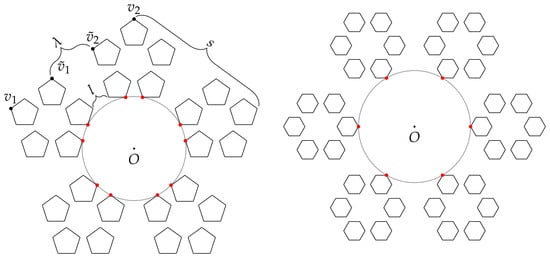
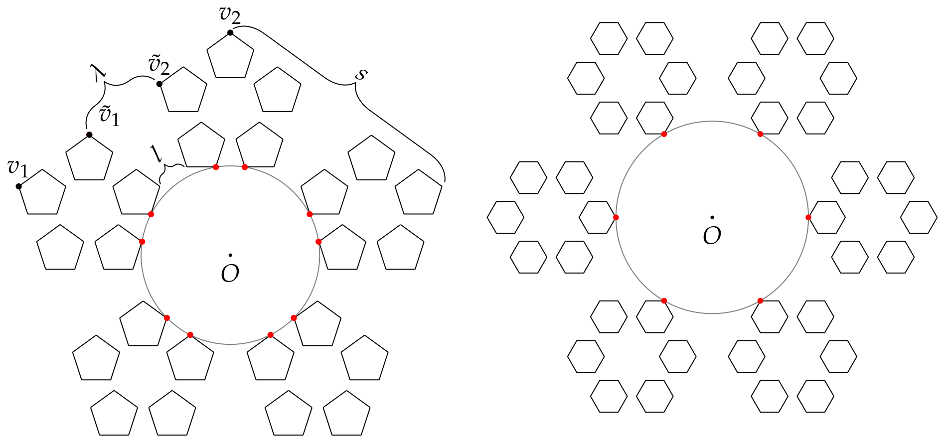
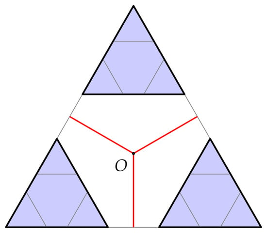
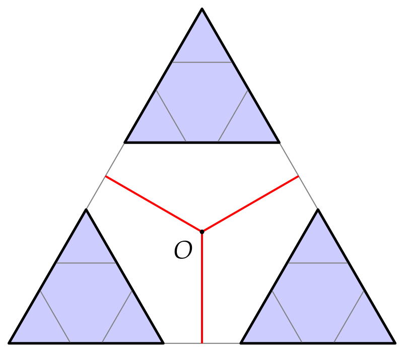
Further let be $K:=\mathrm{conv}\left(\{V_1,\dots ,V_n\}\right)$ the convex hull of $\{V_1,\dots ,V_n\}$, where $V_1,\dots ,V_n$ are the vertices of the underlying n-gon, see Section 3. Because of $g=\sup \{\epsilon >0:{\mathcal{F}}_{\epsilon }\mathrm{has}\mathrm{a}\mathrm{hole}\}$, there is only one element in ${\mathrm{Hp}}_g\left(\mathcal{F}\right)=\left\{O\right\}$, the centroid of $\mathcal{F}$. Thus the set ${\Pi }_O$ has n elements if a vertex of ${\mathcal{S}}_{1}K$ has the closest distance to the centroid of $\mathcal{F}$; otherwise, it has $2n$ elements (see Figure 6). In particular, ${\Pi }_O$ is a finite set.

Figure 6. Elements of ${\Pi }_O$ (red) for $n=5$ (left, 10 elements) and $n=6$ (right, 6 elements).

Step 2: Claim. The value $g\in \mathrm{Hv}\left(\mathcal{F}\right)$ is isolated.

By self-similarity of $\mathcal{F}$ it is enough to look at hole points $\tilde{c}\in K\setminus \left({\bigcup }_{i=1}^n{\mathcal{S}}_{i}K\right)$. Note that then it holds $\tilde{c}\in \mathrm{Unp}{\left({\bigcup }_{i=1}^n{\mathcal{S}}_{i}K\right)}^{\mathsf{c}}\cap K$, where for $F\in \mathcal{H}\left({\mathbb{R}}^d\right)$$\mathrm{Unp}\left(F\right)$ denote the set of points in ${\mathbb{R}}^d$ having a unique nearest point in F. Observe that the centroid O (by Step 1 the only element in ${\mathrm{Hp}}_g\left(\mathcal{F}\right)$) is the point in $\mathrm{Unp}{\left({\bigcup }_{i=1}^n{\mathcal{S}}_{i}K\right)}^{\mathsf{c}}\cap K$ having the largest distance to $\mathcal{F}$ (see Figure 7). If n is odd, the centroid is also centered to the biggest gaps of $\left(\overline{K\setminus {\bigcup }_{i=1}^n{S}_{i}K}\right)\cap \mathcal{F}$; therefore g is isolated in $\mathrm{Hv}\left(\mathcal{F}\right)$ (see Figure 6). If n is even, vertices of ${\mathcal{S}}_{1}K$ have the closest distance to the centroid of $\mathcal{F}$ and therefore g is isolated. In both cases it is $g\le 1-2r$, $s:=|\overline{V_1{V}_2|}=2\sin (\pi /n)$ and $\lambda :=|\overline{{\tilde{V}}_1{\tilde{V}}_2}|=s-2rs$, with ${\tilde{V}}_1:=V_1+r(V_2-V_1)$ and ${\tilde{V}}_2:=V_2+r(V_1-V_2)$, see Figure 6. Therefore it is clear that $2g>\lambda$; thus, g is isolated.

Figure 7. The set $\mathrm{Unp}{\left({\bigcup }_{i=1}^n{S}_{i}K\right)}^{\mathsf{c}}\cap K$ (red) for $n=3$.

Step 3: From Step 2 there exists a $\delta >0$ such that ${\mathcal{F}}_{\epsilon }$ has exactly one hole for $\epsilon \in (g-\delta ,g)$. From Step 1 we see that for $\epsilon \in (g-\delta ,g)$ the hole of ${\mathcal{F}}_{\epsilon }$ is the same as the hole of ${\left({\Pi }_O\right)}_{\epsilon }$. But then the area of the hole is with Lemma 4 given by the function $H:(g-\delta ,\infty )\to [0,\infty ),\epsilon \mapsto H\left(\epsilon \right)$ that has no second derivative in g.

Step 4: Claim. The function ${\lambda }^2\left({\mathcal{F}}_{\epsilon }\right)$ is not smooth at g.

Let ${\mathcal{F}}^{*}:=\mathcal{F}\cup B(O,g)$. By Step 3, for $\epsilon >g-\delta$ we have

$${\lambda }^2\left({\mathcal{F}}_{\epsilon }\right)={\lambda }^2\left({\mathcal{F}}_{\epsilon }^{*}\right)-H\left(\epsilon \right).$$

(9)

We assume that ${\lambda }^2\left({\mathcal{F}}_{\epsilon }^{*}\right)\in C^2((g-\delta ,l)\setminus \left\{g\right\}).$ We will show that then ${\lambda }^2\left({\mathcal{F}}_{\epsilon }^{*}\right)\in C^2\left((g-\delta ,l)\right)$ holds: By Theorem 4, we have

$${\lambda }^2\left({\mathcal{F}}_{\epsilon }^{*}\right)\in C^2((g-\delta ,l)\setminus \left\{g\right\})\iff {\mathcal{H}}^1(\partial {\mathcal{F}}_{\epsilon }^{*})\in C^1((g-\delta ,l)\setminus \left\{g\right\})$$

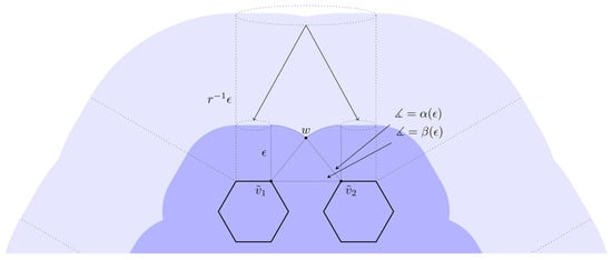
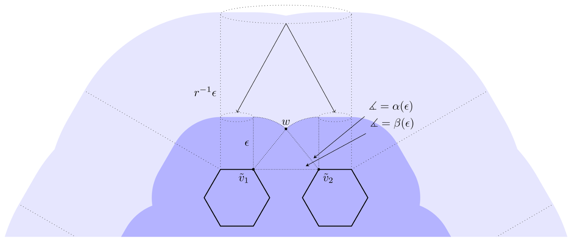
and thus it is enough to show that ${\mathcal{H}}^1(\partial {\mathcal{F}}_{\epsilon }^{*})\in C^1\left((g-\delta ,l)\right).$ As illustrated in Figure 8, by the self-similarity of $\mathcal{F}$, it holds that

$${\mathcal{H}}^1(\partial {\mathcal{F}}_{\epsilon }^{*})=r·2·\left[{\mathcal{H}}^1(\partial {\mathcal{F}}_{r^{-1}\epsilon }^{*})-r^{-1}·2\epsilon \pi \right]+2\epsilon \pi +R\left(\epsilon \right)\forall \epsilon \in (g-\delta ,l/\left(2r\right)).$$

(10)

Figure 8. Schematic setup for Equation (10) and the calculation of $R\left(\epsilon \right)$.

By assumption, the first summand in Equation (10) is $C^1\left((g-\delta ,l)\right)$. The third summand $R\left(\epsilon \right)$ is given by

$$R\left(\epsilon \right)=2n·\epsilon ·\alpha \left(\epsilon \right)\forall \epsilon \in (g-\delta ,l/(2r\left)\right),$$

where $\alpha \left(\epsilon \right):=\pi /2-\beta \left(\epsilon \right)$ with $\beta \left(\epsilon \right):=\angle {\tilde{V}}_1{\tilde{V}}_{2}w$. Here, w is the intersection point of the perpendicular bisector of $\overline{{\tilde{V}}_1{\tilde{V}}_2}$ and $\partial {\mathcal{F}}_{\epsilon }$ that is closest to $\overline{{\tilde{V}}_1{\tilde{V}}_2}$ (see Figure 8). Clearly,

$$\beta \left(\epsilon \right)=\arccos \left({\displaystyle \frac{|\overline{{\tilde{V}}_1{\tilde{V}}_2}|}{2\epsilon }}\right)\forall \epsilon \in (g-\delta ,l/\left(2r\right)).$$

Thus, $R\left(\epsilon \right)$ is a $C^1\left((g-\delta ,l)\right)$ function, which implies that ${\lambda }^2\left({\mathcal{F}}_{\epsilon }^{*}\right)\in C^2\left((g-\delta ,l)\right)$. Consequently, by Equation (9), Lemma 4 and Remark 6, ${\lambda }^2\left({\mathcal{F}}_{\epsilon }\right)$ is not smooth at g. By Proposition 1, this concludes that $\mathcal{F}$ is not Minkowski measurable. □

Remark 8.

For $n=4$ and $r<1/2$, we have $F^{n,r}=C^{1/r}$, the Cantor dust set discussed in [8]. The main result of [8] states that $C^{1/r}$ is not Minkowski measurable for $r\le 1/30$. For $1/30<r<1/2$, it is only conjectured (and supported by numerical evidence) that $C^{1/r}$ is not Minkowski measurable.

Remark 9.

Note that if $r=R_n$, then the attractor is a Sierpinski n-gons (for $n=3$ the classical Sierpinski Triangle). In this case the function $f\left(\epsilon \right)={\displaystyle \frac{{\lambda }^2\left({\mathcal{F}}_{\epsilon }\right)}{{\epsilon }^{2-D}}}$ is not periodic, cf. Proposition 1.

References

- Lapidus, M.L. Vibrations of fractal drums, the Riemann hypothesis, waves in fractal media and the Weyl-Berry conjecture. In Ordinary and Partial Differential Equations, Vol. IV (Dundee, 1992); Pitman Research Notes in Mathematics Series; Longman Sci. Tech.: Harlow, UK, 1993; Volume 289, pp. 126–209. [Google Scholar]
- Gatzouras, D. Lacunarity of self-similar and stochastically self-similar sets. Trans. Am. Math. Soc. 2000, 352, 1953–1983. [Google Scholar] [CrossRef] [Scilit]
- Falconer, K.J. On the Minkowski measurability of fractals. Proc. Am. Math. Soc. 1995, 123, 1115–1124. [Google Scholar] [CrossRef] [Scilit]
- Kombrink, S.; Winter, S. Lattice self-similar sets on the real line are not Minkowski measurable. Ergod. Theory Dyn. Syst. 2020, 40, 221–232. [Google Scholar] [CrossRef] [Scilit]
- Kombrink, S. A survey on Minkowski measurability of self-similar and self-conformal fractals in ℝd. In Fractal Geometry and Dynamical Systems in Pure and Applied Mathematics. I. Fractals in Pure Mathematics; Contemporary Mathematics; American Mathematical Society: Providence, RI, USA, 2013; Volume 600, pp. 135–159. [Google Scholar] [CrossRef] [Scilit]
- Kombrink, S.; Pearse, E.P.J.; Winter, S. Lattice-type self-similar sets with pluriphase generators fail to be Minkowski measurable. Math. Z. 2016, 283, 1049–1070. [Google Scholar] [CrossRef] [Scilit][Green Version]
- Falconer, K. Fractal Geometry: Mathematical Foundations and Applications, 2nd ed.; John Wiley & Sons, Inc.: Hoboken, NJ, USA, 2003; pp. xxviii+337. [Google Scholar] [CrossRef] [Scilit]
- Freiberg, U.; Lippold, J. Family of Non-Minkowski Measurable Fractals in ℝ2. Geometry 2026, 3, 3. [Google Scholar] [CrossRef] [Scilit]
- Hutchinson, J. Fractals and Self-Similarity. Indiana Univ. Math. J. 1981, 30, 713–747. [Google Scholar]
- Schief, A. Separation properties for self-similar sets. Proc. Am. Math. Soc. 1994, 122, 111–115. [Google Scholar] [CrossRef] [Scilit]
- Pearse, E.P.J.; Winter, S. Geometry of canonical self-similar tilings. Rocky Mt. J. Math. 2012, 42, 1327–1357. [Google Scholar] [CrossRef] [Scilit]
- Winter, S. Minkowski content and fractal curvatures of self-similar tilings and generator formulas for self-similar sets. Adv. Math. 2015, 274, 285–322. [Google Scholar] [CrossRef] [Scilit]
- Clarke, F.H. Optimization and Nonsmooth Analysis; Canadian Mathematical Society Series of Monographs and Advanced Texts; John Wiley & Sons, Inc.: New York, NY, USA, 1983; pp. xiii+308. [Google Scholar]
- Clarke, F.H. Generalized gradients and applications. Trans. Am. Math. Soc. 1975, 205, 247–262. [Google Scholar] [CrossRef] [Scilit] [PubMed]
- Fu, J.H.G. Tubular neighborhoods in Euclidean spaces. Duke Math. J. 1985, 52, 1025–1046. [Google Scholar] [CrossRef] [Scilit]
- Schlicker, S.; Dennis, K. Sierpinski n-GONS. Pi Mu Epsil. J. 1995, 10, 81–89. [Google Scholar]
- Rataj, J.; Winter, S. On volume and surface area of parallel sets. Indiana Univ. Math. J. 2010, 59, 1661–1685. [Google Scholar] [CrossRef] [Scilit]
- Stachó, L.L. On the volume function of parallel sets. Acta Sci. Math. 1976, 38, 365–374. [Google Scholar]
- Hug, D.; Last, G.; Weil, W. A local Steiner-type formula for general closed sets and applications. Math. Z. 2004, 246, 237–272. [Google Scholar] [CrossRef] [Scilit]
Disclaimer/Publisher’s Note: The statements, opinions and data contained in all publications are solely those of the individual author(s) and contributor(s) and not of MDPI and/or the editor(s). MDPI and/or the editor(s) disclaim responsibility for any injury to people or property resulting from any ideas, methods, instructions or products referred to in the content. |
© 2026 by the authors. Licensee MDPI, Basel, Switzerland. This article is an open access article distributed under the terms and conditions of the Creative Commons Attribution (CC BY) license.