


Abstract
In both experimental and theoretical analyses of data, we often look to select a set of simple components that can be combined to create an appropriate model for the data. A convenient way to do this is to use quantile functions that can be added or transformed to obtain new distributions. In this work, we connect quantile statistics and mean absolute deviations (MADs) by deriving a general class of MAD-based shape metrics expressed as integrals of the quantile function, with a direct geometric interpretation. Our approach is applicable to distributions with finite mean that include many of the commonly used distributions, including those without a variance, such as the Pareto. When simple midpoint quadrature is used, the proposed metrics recover widely used quantile-shape metrics, including the interquartile range, Galton skewness, and Moore’s octile kurtosis as special cases. We further propose a C-Trapezoid quadrature approximation that combines cubic polynomial endpoint extrapolation with trapezoidal integration, achieving approximation errors that are significantly lower than those of the midpoint approximation for many common distributions. The proposed approximation provides simple-to-compute formulas for shape analysis and yields closed-form, non-iterative parameter-estimation formulas. These formulas are easy to compute and interpret, and they are applicable to a wide class of distributions, including those without an explicit cumulative distribution function or some with heavy tails. Unlike maximum likelihood estimation, the proposed method is more robust and has simple geometric interpretation. We illustrate the methodology with two detailed case studies. The proposed approach gives a simple way to quickly assess distributional shape without any specialized tools.
1. Introduction
In classical statistics, many shape metrics require the computation of the standard deviation. These computations are based on the norm. Such a norm is convenient in differentiation, optimization, and estimation. In addition, as noted in [1], the additive property of variance for independent variables is often cited as one of the prime reasons for its use (for a historical survey, see [2]).
However, standard deviation and other classical shape metrics are sensitive to outliers. An alternative is to use quantile statistics and their quantile shape metrics [3,4], or to use the mean absolute deviation (MAD) or norm. The idea of using such a norm was not new and was used as early as the 18th century by Laplace and Boscovich (for a historical survey, see [5,6], for a survey of more recent results, see [1]).
The -based shape metrics have not been as widely used in statistics as their -based counterparts [1]. However, there is an increased interest in using this norm in statistical studies (e.g., [7,8,9,10,11,12]). Typically, MADs are computed from the density functions [8]. It is also possible to derive MADs by integrating the cumulative distribution function [13]. When a parametric model is well specified, and contamination is mild, maximum likelihood typically retains superior finite-sample efficiency; the octile-based quadrature estimators we develop trade some of that efficiency for closed-form robustness and for geometric interpretability via quantile subareas.
A distinct recent line of work introduces K-moments as an internally consistent alternative to classical raw/central/L-moment systems and highlights their usefulness for dispersion and tail-sensitive inference [14]. Global-scale benchmarking on hydrological margins further compares estimation based on K-moments with maximum likelihood and classical moments [15]. The present MAD-based constructions are complementary: skewness/kurtosis and spread measures here arise from deterministic integrals of the quantile function under explicit quadrature of subareas, yielding octile-level closed forms tied to geometric areas rather than hierarchical moment ladders.
Unless we explicitly mimic dependent data through simulations, finite-sample octiles used in this paper summarize marginally draws after model fitting steps; analyzing long-memory or similarly structured serial dependence [15] lies outside our scope but motivates future extensions. We should note here that other variability metrics exist, such as classical raw and linear moments [16], probability-weighted moments [17], and more recent metrics such as Knowable moments (K-moments—expectations of maxima or minima) introduced in hydrology [18] and discussed in [14]. The methodology of using K-moments is particularly useful in modeling extreme values, where the proposed method has some limitations (discussed in Section 8.6 and Section 8.7). We hope to compare MAD-based analysis with K-moments methodology in the future.
In this work, we connect quantile statistics and MADs by deriving a general class of MAD-based shape metrics in terms of the quantile function. The proposed metrics are expressed as integrals of the quantile function and are easy to interpret. The computation of these metrics is reduced to evaluating these integrals, either analytically or by numerical (quadrature) methods. Using very simple quadrature approximations based on quartiles and octiles, the proposed metrics correspond to many widely used quantile metrics. Among the MAD-based metrics introduced are a MAD-based generalization of Moore’s octile kurtosis and Galton skewness.
For the numerical illustrations later in the paper, we use a small set of standard continuous distributions that are widely cited in textbooks and applications and that, taken together, stress different features of quantile shape: bounded support versus unbounded support; symmetry versus skewness; light tails versus heavier tails; and existence of the mean with or without a finite variance (e.g., Pareto with ). This choice is deliberate: it lets readers compare the same quadrature rules under qualitatively different shapes without committing to a single parametric family.
In Section 6 we report exact and approximate values of the proposed MAD-based skewness G and kurtosis K for these same families, so skewness and tail weight can be read off consistently with the approximation experiments. Throughout, the methods we contrast are the elementary quadrature rules for subareas (midpoint, rectangles centered at octiles, and the cubic-endpoint C-trapezoid rule) applied to the same octile inputs, together with, where relevant, likelihood- and moment-based benchmarks in the parameter-estimation discussion.
This paper is organized as follows. In Section 2, we introduce the notation, summarize most commonly used quantile shape metrics, and derive a formula for MADs based on the subarea integrals of the quantile function. In Section 3, we discuss some elementary quadrature approximation methods using quartiles and octiles. In Section 4, we approximate the endpoints with cubic interpolating polynomials and suggest an additional (C-Trapezoid) quadrature approximation formula. In Section 5, we provide numerical comparisons for some commonly used continuous distributions. In Section 6, we propose MAD-based shape metrics, including shape index, skewness, and kurtosis; they coincide with classical quantile metrics under midpoint quadrature but generalize Galton skewness, Groeneveld and Meeden’s skewness coefficient, and Moore’s octile kurtosis in the MAD setting. We also compare the derived metrics with other such metrics based on classical moments and L-moments. In Section 7, we show how the approximations behave under transformations and convex combinations of quantile functions, illustrating skewed logistic models. In Section 8, we derive closed-form octile formulas for estimating parameters via C-Trapezoid subareas and contrast them with maximum likelihood and quartile fitting. We also compare our method to estimation using L-moments. We compare our results for several commonly used distributions. We address the issue of parameter estimation when distributions have multiple parameters. We also discuss the limitations of our approach when dealing with fat-tailed data and suggest some approaches to address such issues. We then illustrate the methodology with two case studies: Section 9 compares overnight versus daytime XLK ETF returns spanning 1999–2025, highlighting technology-sector regimes that parallel earlier S&P 500 diagnostics; Section 10 analyses weight distributions inside several pretrained transformers. Finally, Section 11 summarizes findings and avenues for refinement. Derivational details reside in the Appendix A, Appendix B, Appendix C, Appendix D, Appendix E and Appendix F.
2. Quantile Shape Metrics and Mean Absolute Deviations
Consider a real-valued random variable X on a sample space with density and cumulative distribution function [19]. Let be the quantile function by with . Let denote the corresponding octiles with and for . If X is continuous then . Let , , and denote the first, median, and third quartile, respectively.
Of particular interest are the quantile metrics that use quartiles and octiles [20]. Using the quantile function , we can compute several such quantile measures of shape, including (Galton’s) skewness and (Moore’s) kurtosis. These are summarized in Table 1.
Table 1.
Quantile measures of shape.
In classical statistics, one computes different shape metrics based on standard deviation and higher-order moments [21,22]. By contrast, in this paper, we will consider several shape metrics based on MAD. These metrics will be expressed as integrals of the quantile functions. Using simple quadrature approximations, we will show that these measures correspond to many of the quantile metrics in Table 1. Moreover, we will consider approximations of these integrals and obtain more accurate estimates of these shape metrics, including improvements to Moore’s kurtosis formula.
We will confine ourselves to continuous distributions. For such distributions, is monotonically increasing. Let denote the mean of X and let M denote the median of X. We will assume the existence of the first-order moment . In such a case, for any real-value a, define MAD of X from a as [7]
MAD is an -metric for measuring the spread of data and is analogous to the standard deviation metric used in classical statistics [16]. It is well-known [7,23,24] that for any distribution with finite variance . On the other hand, MADs require only the existence of the first-order moment. We can rewrite the above Equation (1) for in terms of the quantile function . Since and , we have . Therefore,
In particular, the mean of the distribution
It has a simple interpretation as the area under the quantile function and is shown in Figure 1a.
Figure 1.
Area interpretation of mean and MAD as areas.
We will introduce the following notation. For , define:
Then we can rewrite the above equation as
Note that for any , the mean is
For MAD around the median , we have
This can be rewritten as
Alternatively, to compute MAD around each octile , Equation (4) can be rewritten as
For MAD around the mean , let and
In this work, we will focus on MAD around the median and quartiles [25]. We will use the notation for convenience. From Equation (8), the MAD H of X around the median can be interpreted as the difference between corresponding subareas. Note that we can also rewrite the expression for H as
and interpret H as the sum of two areas. This is shown in Figure 1b.
Let us define the left and right subareas and of X as
Then the MAD H and the mean can written as
Formulae for MAD H and for some common distributions are presented in Appendix B. By analogy to the coefficient of variation in classical statistics, we can define the MAD-based Relative Dispersion RD as
Example 1.
Suppose X is distributed according to an exponential distribution with rate [21]. Its density and cumulative distribution function are
The quantile function is with octiles . The auxiliary integral is
Therefore, for the subareas, we obtain and . Then from Equation (14) we obtain that MAD H around the median is and its mean . Note that for this distribution, the MAD H coincides with the median . Since , for this distribution , and, therefore, this distribution is non-symmetric and is right-skewed with a high concentration of lower data points on the left and a long, thin tail on the right.
3. Quadrature Approximations to Subareas
In this paper, we demonstrate that many shape metrics can be expressed as MAD around specific (primarily quartile) values. These MAD measures require the computation of subareas (integrals) under the quantile function. We consider several simple quadrature approximations to such integrals and demonstrate that many commonly used quantile metrics of shape correspond to straightforward quadrature methods.
In quadrature approximation, we replace the integral with a weighted sum of quantile values, the so-called “abscissas” or “Quadrature points” [26]. Since or can be unbounded, we will first confine ourselves to very simple rules, mostly the “rectangular” quadrature approximations [27]. We will show that even these simple rules provide valuable insights into interpreting the shape metrics. In Section 4, we approximate the endpoints with cubic polynomials and consider trapezoid quadrature approximation that will be shown to give a much lower approximation error.
We start with two simple quadrature approximations for the mean and MAD H. For notational convenience, let us introduce the subarea integrals between successive quartiles:
Note that with this notation, and .
3.1. Midpoint Quadrature Approximation
We start by using the midpoint approximation, which involves a single rectangle of height and width for the left and right subareas. With a midpoint approximation, for each subarea integrals, we have and . With this approximation, and . With this approximation, MAD H is approximated by the interquartile range. This is shown in Figure 2b.
Figure 2.
Quadrature approximation methods for subareas.
In the midpoint approximation, the relative dispersion is the IQR divided by the median . This MAD-based robust alternative is simpler than the coefficient of variation used in classical statistics.
Example 2.
For exponential distribution, the exact mean whereas a midpoint approximation is . This represents about 67% relative error. The exact MAD is whereas the midpoint approximation gives . This represents a 60% relative error.
3.2. Rectangles Quadrature Approximation
We consider approximating left and right subareas and in Figure 1 by four rectangles centered at octiles and :
Then and . This is shown in Figure 2b. With this approximation, we have
Example 3.
For the exponential distribution, we obtain and . This results in relative errors of 35.9% and 16.0% for MAD and mean, respectively. This represents a much lower relative error than the midpoint approximation.
4. Approximating with Cubic Polynomials
The accuracy of the approximation of the subareas will depend on the quadrature method and on the shape of the quantile function. The approximation methods considered in the previous sections involve areas of rectangles centered at quartiles. Since is a monotonically increasing function, it would seem reasonable that other simple quadrature methods, such as the trapezoidal method, could provide higher accuracy. To use such methods to compute and , we would need to use and .
However, for many distributions, one or both of these values could be unbounded. To apply quadrature approximations with such values, we propose to estimate and using octiles only. One of the simplest ways to accomplish this is to consider cubic polynomial curves and passing through reference points corresponding to octiles in the left and right subareas, We then replace and by and , respectively.
We proceed as follows. For each octile and define the point . We will call these “reference” points. For the left subarea , we have four such points , , and . Similarly, for the right subarea we have sour points , , and . This is illustrated in Figure 3.
Figure 3.
Approximating end points and by cubic polynomials.
To compute these cubic polynomial curves, we use Lagrange’s interpolation formula to construct a polynomial that passes through a set of corresponding reference points [28]. To that end, define Lagrange basis polynomials:
The equation for the curve is then
We will consider using cubic polynomial curves passing through four reference points in the left and right subareas to estimate the endpoints, combined with trapezoidal quadrature.
4.1. Using Cubic Polynomials to Estimate End Points for Trapezoid Integration
Consider a (left) cubic curve passing through the four reference points , , and given by Equation (22). Its value at is
Similarly, consider a (right) cubic curve passing through four reference points: , , and given by Equation (22). Its value at is
Once we have estimates for the endpoints and we consider the trapezoid approximation for the subareas in Equation (18):
With trapezoid approximation, we obtain for the left and right subareas and :
This gives us the following approximations to the MAD H and the mean in terms of octiles:
Example 4.
For the exponential distributions, the estimates for the endpoints are
Note that and practically identical to 0. The right estimated point . The probability mass excluded to the right of this point is , significantly less , the area to the right of the octile. With the trapezoid approximation in Equation (27) we have . This results in a relative error of approximately for MAD. This is significantly better than previously considered methods for the exponential distribution.
We will call this method of combining endpoints and (estimated by cubic polynomials) and trapezoid quadrature, a “C-Trapezoid” method. Its accuracy for many distributions will be discussed in the next sections.
4.2. Probability Mass Excluded by Cubic-Approximated Endpoints
When using cubic polynomial interpolation to approximate the endpoints and from interior octiles, it is important to understand how much probability mass lies outside the approximated endpoints. This provides insight into the truncation error introduced by the endpoint extrapolation used in the quadrature rules.
For a continuous distribution with cumulative distribution function , we measure the probability mass that lies outside the approximated endpoints. When the approximated left endpoint is greater than the true , the excluded mass to the left is
which represents the probability mass that falls at or below the approximated endpoint (and, thus, outside the true support if ). Similarly, when the approximated right endpoint is less than the true , the excluded mass to the right is
which represents the probability mass that falls strictly above the approximated endpoint.
For the true endpoints and , we have and (by definition of the quantile function), so the excluded mass would be zero. Any nonzero values for or represent probability mass that is excluded (truncated) when using the approximations instead of the true support endpoints. Equivalently, the included mass is on the left and on the right.
In Table 2, we compute the probability mass to the left and to the right of the proposed cubic approximations and for some well-known distributions. For exact endpoints, both values are zero.
Table 2.
Probability mass excluded by cubic-approximated endpoints.
Examining Table 2, we exclude about 4% in each tail. Several observations can be made:
- For distributions with bounded support (Uniform, Power), cubic interpolation captures the endpoints well, with negligible excluded probability mass.
- For distributions with unbounded support (Normal, Laplace, Exponential, Log-normal, Pareto, Weibull), cubic interpolation excludes a small but nonzero fraction of probability mass (typically on the order of ).
- The excluded mass is generally symmetric for symmetric distributions (Laplace, Normal) and asymmetric for skewed distributions (Exponential, Log-normal, Pareto, Weibull).
- since only octiles are used, the approximation is robust to outliers with a breakpoint of 25% (12.5% at each tail)
Overall, this analysis shows that cubic endpoint construction introduces only modest truncation of probability mass. Given the excellent performance of the C-Trapezoid rule shown in the next Section, this level of truncation error is acceptable in practice, especially when working with empirical quantiles from finite samples. Therefore, we will use these cubic endpoint estimates and in the trapezoid approximation method discussed in Section 3.
5. Approximation Accuracy for Common Distributions
This section compares the accuracy of the proposed quadrature approximations to the subarea integrals and , and hence to the mean and the median MAD , for the distributions listed below. The distributions were selected to cover complementary cases: Uniform (bounded, flat density), Normal and Laplace (unbounded, symmetric, light tails), Log-normal, Weibull and Exponential (unbounded, skewed), and Pareto with (heavy right tail with finite mean but infinite variance). The comparison is methodological: for each distribution, we hold the quantile function fixed and evaluate midpoint quadrature, the octile-rectangle rule, and the C-trapezoid rule, summarized in Table 3, reporting percent error relative to exact integration where available.
Table 3.
Quadrature approximations for subarea integrals.
5.1. Simple Numerical Comparisons
In Table 3 we present the expressions for the subarea integrals obtained by the proposed quadrature approximations.
Example 5.
In Table 4, we illustrate the accuracy of the proposed quadrature approximations for the exponential distribution. Recall that for this distribution, the quantile function with octiles . With the above expressions for octiles of exponential distribution, from Table 3, we can express the quadrature approximations for subareas, shown in Table 4.
Table 4.
Quadrature approximations of subareas for exponential distribution.
As can be seen from Table 4, the C-Trapezoid gives the minimum relative error for both left and right subarea integrals and . The midpoint and rectangle approximation give similar results.
5.2. Comparison of Approximation Accuracy for Common Distributions
We now present the accuracy comparisons for some common (standardized) distributions.
- uniform ( and )
- exponential (with rate )
- Standard Normal ( and )
- LogNormal (with and )
- Laplace (mean and scale )
- Pareto ( and )
- Weibull ( and )
The corresponding approximations for MADs are summarized in Table 5.
Table 5.
Quadrature approximations for MAD H.
To further understand the accuracy of quadrature approximations, we examine the left and right subarea integrals and directly. Table 6 and Table 7 present the true values and estimated values of and , respectively, computed from a single sample of size for each distribution using three quadrature methods: midpoint, rectangles, and C-trapezoid. The true values are computed by numerical integration of the quantile function over the intervals and respectively. These tables demonstrate how each approximation method performs in estimating the fundamental subarea integrals that underlie the mean and mean absolute deviation .
Table 6.
Left subarea integral estimates across distributions using different quadrature methods. True values computed via numerical integration of over . In each row, the green color indicates the best approximation, whereas the red color indicates the worst approximation.
Table 7.
Right subarea integral estimates across distributions using different quadrature methods. True values computed via numerical integration of over . In each row, the green color indicates the best approximation. The red indicates the worst approximation.
The results in Table 6 and Table 7 show that the accuracy of each approximation method varies by distribution and by which subarea ( or ) is being estimated. For symmetric distributions like Laplace and Normal, the quartile and C-Trapezoid methods tend to perform well. For skewed distributions like Exponential and Log-normal, the C-Trapezoid method generally provides better estimates of (the right subarea), which is critical for accurate MAD estimation since . For most distributions, the C-trapezoid gives the best approximation. By contrast, the midpoint method, while simple, consistently underestimates both subareas for most distributions, leading to poor MAD estimates as seen in Table 8.
Table 8.
Mean absolute deviation (MAD) estimates and percent error across distributions. Green indicates the lowest error, and red indicates the highest percent error.
In Table 8, we compare the MAD H results for all approximation methods.
Table 8 shows that across all distributions, C-Trapezoid attains smaller errors than both Midpoint and Rectangle rules.
6. MAD-Based Shape Metrics: Computation and Interpretation
We now consider several MAD-based shape metrics. Many of these metrics would correspond to well-known quantiles shape metrics when simple quadrature approximation methods are used. In the computation of these metrics, we will use MAD using only the values to the left and right of the median . We will find it convenient to express these metrics via the mean absolute deviations of truncated distributions.
To proceed, let and denote truncated random variables (with truncation at the median ). We will refer to these as derived left and right random variables. Let , and denote the corresponding density, cumulative distribution, and quantile function for the left derived variable . Similarly, let , and denote the corresponding density, cumulative distribution, and quantile function for the right derived variable .
Because the truncation is done at the median , we have for the left and right random variables and :
For any point a, we have for the MAD of and around a:
6.1. Left and Right Mean Absolute Deviations
Consider the MAD of and of and around and , respectively. Then from Equation (32) we immediately obtain
From the above Equation (33) and Table 3 for quadrature approximations to and , we can compute the quadrature approximations to these left and right MAD. These approximations for p-differences are summarized in Table 9.
Table 9.
Quadrature approximations for MAD and .
Example 6.
For the exponential distribution, , and . Therefore, and .
The MAD is the average distance between and the third quartile . Similarly, the MAD is the average distance between and the first quartile . The midpoint approximation to these distances is the upper and lower q-distances in Table 1.
6.2. Skewness Shape Metrics
Consider the MAD of and around . From Equation (32), for we have
We define the left and right normalized deviations and of truncated left and right variables and around the median . We define MAD skewness G as the difference of these normalized deviations:
Since and from Equation (34) It immediately follows that . This is unlike the Pearson skewness in classical statistics, which could be unbounded. The MAD-based skewness can be used directly to compare any two distributions. In terms of subarea integrals, we can have
Since , Using from Equations (35) and (36) we obtain
The term is the Groeneveld and Meeden’s or Yule’s skewness coefficient [29,30]. This skewness coefficient has a simple interpretation as the ratio of two distances: the numerator is the (signed) distance between the mean and the median , whereas the denominator H is one half of the average distance of values in X to the median . This is an easier interpretation than the classical skewness defined in terms of the central third moment and standard deviation [31].
Using the quadrature approximations in Table 3, for the subarea integrals and , we can approximate the MAD skew in terms of octiles. Quadrature approximations for skewness are summarized in Table 10.
Table 10.
Quadrature approximations for MAD-based skewness G.
The midpoint approximation is the so-called Galton skewness [32]. Therefore, the Galton skewness in quantile statistics can be interpreted as the normalized difference of MAD for right and left truncated variables and distributions from the median , when a simple midpoint approximation for subareas is used.
Example 7.
For the exponential distribution, we have and . The median and . The skewness is then .
6.3. MAD-Based Kurtosis
Let us consider the MAD of and around and , respectively. For notational convenience, let and denote these corresponding “left” and “right” MAD:
The medians of left and right random variables and are and , respectively. It is easy to show that we can express the left and right MAD and as:
The terms and can be interpreted as the average distances between values in and from their respective medians. We can think os these as measuring the “fatness” of left and right tails of X, somewhat similar to the notion of kurtosis in classical statistics [16,33]. We can think of as a normalized MAD-based measure of the left tail and as a normalized MAD-based measure of the right tail. With this in mind, we define MAD-based kurtosis K as the average of these “normalized” tails:
Mad-based kurtosis K in Equation (40) can be interpreted as the average distances between values in and from their respective medians and divided by an average distance of points in X from their median . This gives a simple MAD-centered view of the classical kurtosis measure.
Quadrature approximations for kurtosis are summarized in Table 11. Note that with a midpoint approximation, we obtain the so-called octile kurtosis suggested by Moore [34].
Table 11.
Quadrature approximations for MAD-based kurtosis.
It is interesting to note that Moore suggested his formula based on the following analogy to classical kurtosis . If denotes the standardized random variable and , then and and, therefore, . The classical kurtosis can be viewed as related to the dispersion of around its mean 1, or equivalently, with the dispersion of Z around and 1 [34]. This implies that classical kurtosis is associated with the concentration of X around points and respectively.
With this analogy, an quantile alternative K to classical kurtosis was suggested in [35] in terms of the inter-quartile ranges and around corresponding medians and using octiles . The MAD-based kurtosis K in the above Equation (40) measures the MAD of and from their corresponding medians and , playing the role of as in classical statistics.
Example 8.
For the exponential distribution, . For the left and right MAD, we have and . Skewness and kurtosis .
It is well known that MAD is minimized by the median [23,24]. Therefore,
This gives the following upper bound for MAD-based kurtosis:
Therefore, unlike the classical kurtosis that can be unbounded, MAD-based kurtosis always satisfies . This allows a direct comparison across distributions.
In Table 12 we summarize the values of MAD-based skew and kurtosis computed for some common distributions. The details of the computations are provided in the Appendix A, Appendix B, Appendix C and Appendix D. A further comparison with classical skew and kurtosis can be found in [36].
Table 12.
MAD-based skew and kurtosis for common distributions. Here, and are the octiles of the standard normal .
6.4. Comparison with Classical Skewness and Kurtosis
Classical skew and kurtosis are defined as normalized third and fourth central moments:
These are summarized in Table 13 for some common distributions.
Table 13.
Classical skewness and kurtosis for common distributions.
Note for classical kurtosis, [16]. The lower bound is realized by the Bernoulli distribution. The classical kurtosis itself is unbounded. By contrast, for MAD-based skew G and kurtosis K, we have and . Therefore, for any distribution .
6.5. Some Additional Tail Metrics
We defined MAD-based kurtosis as measuring the MAD of and from their respective medians and . We can consider additional metrics of tail weight and tail length, which indicate the degree of probability in the tails of a distribution. One way to assess heavy tails is to measure whether the probability in the outer tails is particularly large or small. A simple way of summarizing the tail length is to use the so-called identification quantile function [4]:
The values of and are compared with and indicate tail lengths. For example, a distribution with is regarded as having a long right tail. If it is between zero and 0.5 then it is regarded as short-tailed.
Example 9.
Consider the exponential distribution with . For this distribution,
From this, we obtain and . Therefore, the exponential distribution has a long right tail and a short left tail.
Another approach to measure skewness and kurtosis is to use L-moment based skewness and L-kurtosis defined in terms of the L-moments discussed in Appendix C for many common distributions.The L-skewness is strictly bounded within the interval . The L kurtosis is strictly bounded in the interval . They are related by the inequality .
Example 10.
Consider the exponential distribution. The L moments for this distribution are , , and . The L-based skewness and L kurtosis is .
Table 14 summarizes L-moment skew and kurtosis for common distributions [37]. The details are presented in Appendix C.
Table 14.
L-moment skewness and kurtosis for some common distributions. Formulas are from [37].
There have been several methods to compare distributions in terms of tails, such as comparing the quantile functions as and other methods [3]. We believe that MAD-based skew G and kurtosis K offer an attractive alternative to these measures: both measures have simple interpretation, simple approximations, and allow direct comparisons across distributions.
6.6. Numerical Comparisons
We now show the accuracy of our approximation. Assume that we have n data points . We compute the octiles . Let be the number of elements less than or equal to and let denote the number of elements greater than .
Then, we can compute the empirical MAD:
From this, we compute the MAD skew . The approximation results for the common distribution are in Table 15. For log-normal, we take and . For Pareto, and .
Table 15.
MAD-based Skewness G approximations across (non-symmetric) distributions using different quadrature methods. In each row, the green color indicates the best approximation, the red color indicates the worst.
Next, we compute MAD-based kurtsois . The results are in Table 16.
Table 16.
MAD-based kurtosis K approximations across distributions using different quadrature methods. In each row, the green color indicates the best approximation, and the red color indicates the worst approximation.
As shown in Table 15, C-Trapezoid achieves the smallest absolute percentage error for skewness G across the three distributions listed. Table 16 is more mixed: for kurtosis K, C-Trapezoid is best on Normal and Laplace, Midpoint on Exponential and Pareto, Rectangles on Log-Normal, while Uniform is essentially exact under both Midpoint and C-Trapezoid (percentage errors rounded to two decimals). Overall, C-Trapezoid remains strongest for skewness in this comparison; no single quadrature rule dominates kurtosis across all six distributions.
6.7. Summary of MAD-Based Shape Metrics
We conclude with a summary of MAD-based shape metrics and their quantile statistics equivalents when a midpoint quadrature approximation is used. For ease of comparison, we follow the same format as Table 1. The results are summarized in Table 17:
Table 17.
Mad-based shape metrics and quantile equivalents.
7. Transformations and Convex Sums
In both experimental and theoretical analyses of data, we often look to select a set of simple components that can be combined to create an appropriate model for the data. A convenient way to do this is to use quantile functions that can be transformed or added to obtain new distributions.
7.1. Transformations
We start with the following result: if is a non-decreasing function of x then is a quantile function [3]. Let and let . Since is non-decreasing, we have
and, therefore, . In other words, the quantile function of the transformed variable z is obtained by transforming the quantile function of the original variable x. Note that for the medians we have
Example 11.
Consider the standard uniform random variable U. Its quantile function is . Consider the function and let . Then Z is exponential with a a quantile function .
The following are common transformations:
- Reflected Distribution: Let Y be the distribution X reflected around . Its quantile function .Then, the quantile function of the reflected distribution Y is . In particular, the octiles of Y are related to octiles of X via . The auxiliary integral of Y is .In particular, and .Example 12(reflected exponential). Let X be the exponential with scale and Y the reflected exponential. The quantile function of X is and the quantile of Y is . Its auxiliary integralIn particular, its MAD and mean are and .
- Power Transformation: for some with .Example 13.X is standard exponential with . Then, Y is a Weibul distribution with .
- Reciprocal Distribution: The quantile function of is .Example 14.Let X be the power distribution . If Y is the reciprocal of X then its quantile function . The distribution Y is a Pareto distribution.
7.2. Convex Sums
- Next, one can consider the (convex) linear combinations of quantile functions. Let be the k quantile functions for variables respectively. For each random variable , let denote the corresponding octiles. Let denote the MAD of around its median and let denote the its mean. Let be non-negative constants with and let
In particular, for the octiles of Z, from Equation (49), we have
For each , define the left and right subarea integrals and as
Then, from Equation (49) we immediately obtain for the MAD of Z around its median, we obtain
Similarly, for the mean of Z we obtain:
Finally, if we use cubic interpolation on four interior octiles of Z to construct the endpoints then from Equations (23), (24) and (50) we obtain
and
Therefore, all our approximation methods via octiles are linear: the corresponding subarea integrals for Z can be approximated by the corresponding weighted sums of individual quadrature approximations with octiles.
Example 15
(skewed logistic). Let and . These are the quantile functions of the exponential distribution X and the reflected exponential distribution Y, respectively. Consider a quantile function of the form
with . This is a quantile function of the skewed logistic distribution [38]. Note that for , we do not have an explicit form for the cumulative distribution function. However, we can use the quantile function to compute shape metrics and to estimate parameters.
The MAD and mean of Z are:
This gives us the following estimates of the parameters of skewed logistic distribution in terms of the left and right subareas and of Z:
The subareas can be approximated using octiles via the quadrature approximations developed in this paper. Table 18 shows estimates of s and w from a single sample of size for two choices of true , using MLE, quartile (two-quartile) approximation of , , and C-trapezoid approximation.
Table 18.
Parameter estimates for the skewed logistic: true vs. MLE, Quartile, and C-Trapezoid ().
As shown in Table 18, the C-trapezoid achieves better accuracy than quantile fitting and provides a quick approximation of the parameters within 10% relative error. By contrast, simple quantile fitting gives a much larger relative error of about 25% (especially in estimating s).
8. Parameter Estimation for Common Distributions
In this section, we illustrate how to compute parameters for common distributions. We derive the expressions for parameters in terms of the auxiliary integrals and . These are, in turn, approximated with the suggested C-trapezoid quadrature approximations.
8.1. Parameter Estimation with C-Trapezoid Approximation
The proposed method of parameter estimation is the following: Assume that we have n data points . We compute the octiles and compute the subarea integrals and with C-trapezoid approximation. We then estimate distribution parameters from these subarea integrals. Details of the computation of parameters for common distributions are presented in the Appendix B.
We compare the proposed MAD-based method for estimating the parameters with the following three common methods:
- Maximum Likelihood Estimation (MLE): this method is widely used and is accurate [39]. It provides efficient estimators with minimal variance [40]. A historical overview is given in [41]. Despite its advantages, MLE lacks closed-form solutions for many distributions [42] and requires iterative methods.
- Moment fitting: this method, formalized by Pearson [43], matches theoretical and empirical moments for computationally accessible estimators. It has limitations with heavy-tailed or asymmetric distributions [44], and the estimates are susceptible to outliers [45,46].
- Quartile fitting: in this method, we derive parameters by matching theoretical and empirical percentiles [47,48].
There are many other methods, including the Bayesian paradigm [49], Maximum entropy methods [50,51] and others [52]. Many of these methods are computationally complex or assume particular distributions. By contrast, the proposed C-trapezoid approximation is simple and non-parametric. Although not as accurate as other methods, it is very simple and gives a close approximation for many common distributions.
Example 16.
For exponential distribution, and . The parameter λ is estimated as or alternatively, . The maximum likelihood estimation is . The moment-fitting estimate is the same as MLE for exponential data. With median (quartile) fitting, and it uses the median only. Finally, with C-trapezoid method, with subareas and estimated by the C-trapezoid octile formula in Equation (68).
Table 19 gives example estimates for the scale for each distribution. Values are mean estimates over 500 replicates with . Percent errors relative to the true value are shown in parentheses.
Table 19.
Estimates for the scale parameter across distributions: True (parameter used in simulation), MLE, Moment-fit, Quartile, and C-Trapezoid. Mean over 500 replicates, . Percent error is shown in parentheses.
Table 19 suggests that MLE and moment fitting are consistently the most accurate in this simulation, quartile fitting has the largest bias, and the proposed C-trapezoid method substantially improves over quartile fitting while remaining less accurate than MLE/moment fitting.
8.2. Comparison with L-Moments
Linear moments (L-moments) are expected values of linear combinations of order statistics. Hosking [37] defines the r-th L-moment as follows. If X is a real-valued random variable, let be the order statistics of size n. Then, the L-moments of X are defined as
It can be shown that these can be expressed as follows
where the functions are shifted Legendre polynomials
The first L moments are:
The first two L-moments and , are called L-location and L-scale. The third and fourth L-moment ratios and are called L-skewness andL-kurtosis. These can be used to summarize a univariate distribution. Note that L-moments are a linear function of the expected order statistics. The existence of a finite mean for X is a necessary and sufficient condition for all linear moments to exist [37].
If a distribution has finite variance , then the following relations hold:
Equation (63) shows that gives more weight to larger differences as these are squared. Since L-moments are linear functions of ordered data, they are less sensitive to outliers, providing more stable shape estimates estimates.
Example 17.
For the exponential distribution, the first L-moments are:
If we have a sample of size n drawn from a distribution specified by a finite number k of parameters, then we estimate these parameters by equating the first k sample L-moments to corresponding population estimates. Such methods offer robust alternatives to traditional measures of standard deviation, skewness, and kurtosis. In small sizes, this method can outperform maximum likelihood estimation for some distributions. For a detailed discussion, see [53,54].
It is of interest, therefore, to compare this method to the parameter estimation based on MADs. In Appendix C, we summarized the parameter estimation method based on L-moments. Since L-moments are expressed as integrals of products of quantile functions with polynomials, we could consider approximating L-moments using the C-trapezoid approximation. Let us define as the integrand of in Equation (62).
Then, if we define and and, then C-trapezoid approximation for the r-th linear moment in Equation (60) is
Equation (64) gives us a unified way to compute the L-moments directly in terms of octiles and polynomials evaluated at .
To illustrate, consider the computation of the first two L moments and . Since is it clear that the first linear moment is just the mean . Then, from Equation (27) we obtain
Next, for we have . Then replacing by and by we have
Then, the C-trapezoid approximation for the second L-moment gives us
Once L-moments are (approximately) computed, we can use them to estimate the parameters. We can also estimate the parameters via subareas and . Recall that the C-trapezoid approximation for the left and right subareas and from Equation (68):
We summarize parameter estimation using L moments and MAD (using subarea integrals) in Table 20.
Table 20.
Comparison of parameter estimation using L-moments ( and ) and subarea integrals ( and ) for some common distributions.
Finally, let us connect the L-moments and auxiliary integral as follows. Since a simple integration by parts gives
Alternatively, consider Equation (6). For any we have
Integrating both sides of Equation (70) we obtain
From Equations (69) and (71), we obtain
Equation (72) gives us a very simple interpretation of the second linear moment: The second linear moment is one-half of the integral of MADs computed over all points.
Table 21 summarizes one draw (default_rng(42)): formulas of Table 20 with PWM-based [37] vs. trapezoid (68) from linear interpolated octiles (extrapolated last bin).
Table 21.
Comparison of estimates for scale of L-moment and MAD-based estimation with C-trapezoid approximation ( points). Parentheses show absolute percent error relative to the true scale parameter with C-trapezoid approximation.
Table 21 shows MAD-based method has better accuracy for heavy-tailed distributions like log-normal and Pareto. while remaining competitive for most other distributions.
Example 18.
For the exponential distribution, from Equation (A18) we have . The second L-moment is then
8.3. Estimating Parameters for Distributions with Several Parameters
We can extend our method to handle distributions with several parameters. For common distribution with one or two parameters, we estimated the parameters by computing the analytical expression for the subareas integrals and approximating them in terms of quadrature approximations. For distributions with multiple parameters, it is sometimes easier to compute them via empirical MADs. The key idea is to compute MADs around octiles. For k parameters, we need to use k such equations.
Our general approach is the following. As before, assume that we have n data points . Let be the sample octiles. Define the sample mean and the sample MAD of X around empirical octiles by
This computation of empirical MAD requires subtractions, computing absolute values and additions for each octile. If the empirical octiles are available, then we can approximate MADs from Equation (10) by C-Trapezoid approximation as follows
For notational convenience, we let and be the left and right endpoints and computed from empirical octiles using Equations (23) and (24).
If we use MADs around all octiles, then Equation (73) gives us eight equations: one for the mean and seven for MADs of X around its 7 octiles. We compute the parameters by equating the theoretical expressions for the mean and MAD with their empirical counterparts and : The main equation is the following (from (10))
We illustrate this for some important distributions. Let us consider a few interesting cases:
- Distributions with the same number of parameters and equations: We first consider the case of using exactly k parameters with k equations.Example 19.Assume that X a generalized 4-parameter Tukey distribution [3]. Its quartile functionwhere the parameter is the location, is the scale, is the skewness and is the kurtosis.For this quantile function, we obtain for the auxiliary integralFor the mean and MAD of X around , and we obtain:By equating the analytical expressions for mean and MAD in Equation (78) with their empirical counterparts in Equation (73)and using the C-trapezoid approximation for the integrals in Equation (78), we estimate the parameters , , and . There are four equations and four unknowns. We compute these parameters numerically by standard iterative methods.
- Shifted Distributions: A number of multi-parameter distributions are obtained by a single shift. For such distributions, the parameters can be easily estimated from those of the original distribution.Example 20.X is distributed according to the 3-parameter Log-Normal Distribution , () and . The parameter is the so-called threshold. If then this reduces to the standard log-normal distribution X. This distribution is often used in hydrology and reliability analysis [55,56].Let . Then Y follows the standard log-normal distribution with parameters μ and σ. The quantile function . The auxiliary integrals . Then it can be shown that since MADs are shift invariant, and we have .Then from Equation (A39) in Appendix B we obtainwhere are the octiles of the standard Normal distribution. This gives us eight equations from which we can choose three to compute μ, σ, and ν.
- Distributions with a quantile function in closed form: For such distributions, we can often compute an explicit expression for MADs. These expressions could involve some special functions,Example 21.Consider the Burr XII distribution with shape parameters c andk and scale parameter λ This distribution is often used to model non-normal, heavy-tailed and skewed data in reliability analysis [57], insurance [58], flow levels in hydrology [59], to name just a few. For this becomes the Lomax distribution. For we obtain a log-logistic distribution. The details are provided in Appendix D. We summarize just a few results.The quantile function is available in closed form and isThe mean μ and its MAD around octiles are given bywhere and are Beta and incomplete Beta functions respectively. There are three parameters and eight equations in (82).
- Distributions without quantile function in closed-form: For some distributions like Beta, Gamma, Maxwell–Boltzmann [21] there is no closed-form formula for the quantile function. However, these distributions have closed-form expressions for their cumulative distribution functions . In such cases, we use an estimate of the octiles and compute the MAD by integrating the CDF directly. Our main result is the following equation for MAD derived in Appendix E.Example 22.Assume X is distributed according to Gamma distribution with shape parameter and rate [21]. For this distribution, the quantile function does not exist in closed form. We compute mean and MADs by integrating using Equation (83). The details are provided in Appendix E. For this distribution, the mean and MAD areSimilarly, we can compute other MAD for this distribution. Assuming that we can accurately compute the octiles, Equation (84) gives us eight equations for the two unknowns that can be solved numerically. For a survey of methods, see [60],
For many of the cases discussed, we have more equations than parameters. The system is, therefore, over-constrained and will not, in general, have a unique solution. There are a few ways to address this:
- We can choose just k equations for k unknowns. For example, for the 4-parameter Tukey distribution, we took the equation for the mean and three MADs around the quartiles. An interesting question to investigate is what MADs to use (e.g., MADs over “furthest” octiles) or whether it is better to exclude the equation for the mean and just focus on octiles.
- We can choose different sets of k equations, compute the parameters, and average them. For example, for distributions, 3 parameters and 8 possible equations to choose from, there are possible sets of parameters to choose from. We can average over any set of such parameters. The main disadvantage is the computational cost to compute each set. An interesting question to consider is estimating the number of such sets and which sets of parameters to use for averaging.
- We can estimate the parameters by minimizing the mean square error (MSE). To that end, consider the following quadratic “loss” function:We included in and to emphasize their dependence on this parameter. We can compute the parameter by minimizing the loss function . We can use any standard techniques, such as gradient descent [61,62] (for a recent survey, see [63]). For such algorithms, the gradients can be computed numerically by forward differences.
- We can estimate the parameters by minimizing the mean absolute error (MAE). To that end, consider the following “loss” function:Minimizing loss function in Equation (86) is more difficult and sually slower that minimizing quadratic function in Equation (85). The absolute value terms in Equation (86) are not differentiable at zero. This makes it difficult to use many algorithms, such as gradient descent. A detailed discussion is presented in [64].
We hope to investigate these methods and the questions they raise in our future work.
8.4. Comparison to Estimation of Parameters by Truncation
In the suggested C-trapezoid approximation, we use cubic polynomials to truncate at and . A natural question is the following: what if we simply truncate at first and last octile, compute the MAD, and estimate the parameters. How do the obtained approximations compare with the suggested method?
We proceed as follows: Consider a distribution X truncated at and . We will denote this distribution . The density and cumulative distribution function of the truncated distribution are
For any with we can compute MAD as
We now consider some special cases for truncation at the octiles and . The cumulative distribution function of a truncated distribution is . In particular, the median of the truncated distribution
coincides with the median of the truncated distribution.
The mean and MAD around the median for the truncated distribution are
Using the trapezoid quadrature approximation for the integrals:
we obtain the following approximations
Example 23.
Consider the exponential random variable truncated at the first and last octiles. Its density and its cumulative function .
As a supplementary single-draw illustration, we evaluate the truncated-subarea rate estimator from (94) at the empirical octiles of one simulated sample (): this gives , i.e., error relative to . For contrast, Table 19 (exponential row, means over 500 such replicates at ) reports for MLE, for quartile matching, and for the C-trapezoid inversion of . Thus, the truncated-subarea value is much larger than the pooled MLE bias, somewhat larger than the pooled C-trapezoid bias, and closer in magnitude to the pooled quartile bias, underscoring that one realization need not resemble replicate-averaged performance. Therefore, MAD-based estimation with the C-trapezoid is better than simple truncation.
8.5. Tail Probabilities
Using MADs allows estimation of tail probabilities. The most general bound for any distribution (with finite variance ) is Chebyshev’s inequality [16]:
This inequality follows from the so-called Pearson inequality [16] with :
For , we have an inequality for bounds in terms of MAD around the mean
Similarly, there is an inequality in terms of MAD H around the median given by [1]
This inequality does not require a finite variance, only the existence of a Riemann-integrable quantile function , providing a robust alternative across diverse distributional families.
8.6. Advantages and Limitations of Proposed Approximation for Parameter Estimation
Maximum Likelihood Estimation often encounters severe computational difficulties with heavy-tailed distributions, including extremely flat likelihood surfaces and high sensitivity to outliers. When datasets contain measurement errors or outliers, traditional methods such as maximum likelihood or moment fitting can produce severely biased estimates. The proposed approach uses only octiles, providing natural robustness without requiring outlier removal procedures.
As shown above, parameter estimation using the C-trapezoid is not as accurate as maximum likelihood, but it is typically within 10% of the exact values. At the same time, the proposed approximation provides a closed-form, non-iterative formula that is more robust than maximum likelihood or moment fitting, which are more sensitive to outliers. We also note that the C-trapezoid method provides much better parameter estimation than simple median matching. This can be explained by the fact that we estimate parameters by averaging octiles rather than fitting a single value. On the other hand, unlike MLE and moment fitting, we require only octiles, making our method more resilient to outliers.
Example 24.
Consider estimating the parameter λ for the exponential distribution. If we replace the maximum value by then the sample mean doubles and the rate λ decreases by 50%. At the same time, the octiles do not change, resulting in no change for our estimation of λ with octiles using the C-trapezoid method.
Another challenge in applying the proposed method is computing quantiles [65,66]. For large data sets, sorting could be expensive. Sorting algorithms (merge or heapsort and their variants) have complexity [67]. In small data sets, estimates could be sensitive to outliers. There may be dependencies in sequences that are difficult to identify. A detailed discussion on practical and theoretical issues is presented in [65]. A comprehensive review of quantile estimation methods and a methodology for estimating quantiles by simulating processes with arbitrary dependence structures is presented in [68].
The main advantage of our method is its computational simplicity. For many distributions, the method provides a closed-form, non-iterative approximation to the parameters directly in terms of the octiles. A parameter estimation method based on MAD of a truncated distribution using quantile functions was recently described in [69].
Remark (wall-clock comparison). In addition to the asymptotic sorting discussion above, we report illustrative median wall-clock times (milliseconds) for a representative setting in Table 22. For the reported results, maximum likelihood uses iterative optimization while a closed-form, rank-based estimator avoids it. We simulate samples, and for each sample size n we draw independent datasets (seed 0), timing one call per draw.
Table 22.
Illustrative wall-clock times (median ms per independent sample; Weibull , ). MLE via scipy weibull_min.fit (floc); closed-form via Hosking PWM/L-moments + algebraic inversion. , seed 0. Medians are from one representative workstation run; re-run wall_clock_mle_vs_closed_form.py from the public GitHub version 3.5.8. The repository is listed under Data Availability for machine-specific timings.
Baseline (MLE): scipy.stats.weibull_min.fit with fixed location (SciPy 1.16.3).
Closed-form Comparator: unbiased probability-weighted moments [37] for followed by the closed-form Weibull inversion used elsewhere in this paper (sort once per draw; no optimizer).
This comparator matches the computational structure of our octile pipelines—empirical quantiles, fixed linear statistics, and algebraic parameter recovery—while keeping the benchmark narrowly defined and reproducible. The % column is , i.e., the percentage reduction in median time relative to MLE. Full machine metadata, permanent GitHub version 3.5.8. URLs for the replication script and output, and caveats are discussed in Appendix F.
Finally, it should be noted that we do not require the explicit form of the quantile function, only the estimates of the octiles. Some distributions, such as Gamma and Beta, do not have explicit forms for their quantile functions [27,70]. However, many distributions can be modeled by convex linear combinations of quantile functions [3]. Because MAD is based on an metric and additive (Equation (52)), the proposed approximation can be applied directly based on (empirical) octiles.
The proposed methodology of using C-trapezoid approximation provides a unified approach to parameter estimation that is simple, resilient to outliers, and has a simple geometric interpretation. Our approach applies to many distributions (with finite means), including some characterized by heavy tails [71]. Compared with simplistic quantile interpolation, this framework, therefore, improves accuracy broadly, while still requiring readers to heed endpoint-sensitive exceptions such as Laplace. The proposed method yields better results than the commonly used quantile-based methods for most distributions. The main advantage is its computational simplicity and geometric interpretation, which allows a quick initial assessment of candidate models before more advanced analysis methods are employed.
8.7. Limitations with Fat-Tailed Data and Truncation
In our discussion, we assumed that using octiles alone would yield simple expressions connecting mean absolute deviations to shape parameters. The proposed methodology implies truncation at and computed by Equations (23) and (24).
However, there are many applications where the probability in the tails of the distribution can be significant and cannot be ignored. We present two areas:
- Hydrology: as pointed in [3], the occurrence of very long-tailed distributions in hydrology has led to the consideration of specialized quantile functions and distributions [72]. For such models, more specialized methods are often employed, such as K-moment methods [14,15,68]. These methods account for long-range dependence and better handle outlier data.
- Financial Data: Many asset prices in finance do not follow simple distributions [73,74,75]. Starting with pioneering work in [76], several heavy-tail distributions have been proposed, including Levy distributions [77,78,79,80] and their extensions [81,82]. Pareto [83] and other heavy-tailed distributions [75,84].
One of the major limitations of the proposed method is that it involves (implicit) truncation (at and ). As a result, the obtained distributions are not infinitely divisible (i.e., can be expressed as a sum of an arbitrary number of independent and identically distributed random variables). Infinitely divisible distributions are necessary for continuous time asset pricing [73], dynamic portfolio theory [85], and options valuation [86]. Unlike standard normal distributions, infinitely divisible distributions enable the construction of arbitrage-free continuous-time pricing models and allow the modeling of fat tails, large kurtosis [75], and jumps [87].
Although the proposed approximation offers robustness and computational convenience, it may not be feasible for many such distributions. We could extend our methodology to handle such distributions by estimating and for and using these instead of endpoints and .
Another approach is to model such distributions with sums of basic quantile functions considered in this paper. This would allow us to analyze data with fat tails or asymmetry where simple quantile functions would not perform well. We can consider algorithms analogous to expectation maximization or other optimization models to compute the weights. This is analogous to modeling fat-tailed distributions with mixtures of normal distributions. We hope to address this in our future research.
At the same time, we want to emphasize that our goal is to provide a computationally simple method for deciding between models before more advanced analysis methods are deployed.
In the next two sections, we present two case studies to illustrate our approach.
9. Case Study I: Analyzing Overnight and Daytime Returns for Technology Stocks ETF (Exchange-Traded Fund XLK)
For our first case study, we study the similarities and differences in overnight and daytime returns of the XLK Exchange-Traded Fund (ETF). This ETF tracks the largest technology stocks in the S&P 500. We analyze this ETF for 27 years from 1999 to 2025.
It has long been observed that the return distributions in these periods could be quite different for many stocks [88,89,90,91,92,93,94,95,96,97,98,99,100,101]. It should be kept in mind that transaction costs represent a critical factor. Recent research has demonstrated that many documented anomalies disappear after accounting for realistic trading frictions [102,103,104,105,106]. We will ignore trading costs in the current case study.
We will focus on the overnight and daytime returns of technology stocks represented by the XLK ETF. We proceed as follows. For each day , let and denote the Open and Close prices, respectively. These prices are obtained from the Wharton Data Resource Services (WRDS) database [107].
A day consists of two periods:
- (previous) Overnight period: time between the closing time of stock trading of the previous trading day and the opening time of the present day .
- Daytime period: time between the opening time of stock trading for and the closing time of stock trading for the same day .
For the U.S. market, the opening and closing times are the times of the main floor of the New York Stock Exchange: the opening time is 9:30 a.m. EST and the closing time is 4:00 p.m. EST. Although we do have (sometimes active) pre-market and extended hours trading, we will ignore these times and only consider the above times.
Table 23 provides an example of the daily open and close prices and for XLK for several trading days in April of 2024.
Table 23.
Example of historical stock data.
We divide each day into three time periods shown in Figure 4.
Figure 4.
CO (overnight), OC (daytime), and CC (daily) returns over 24-h period.
We compute the corresponding returns for each day and its sub-periods as follows:
- CO (Close-to-Open or “night” trading): this is the return of the first sub-period (night portion) of day . Since this sub-period is the same as the previous night period, its return is computed as the percent change between the Close price at and the Open price of the trading day . We will use the notation to denote such returns.
- OC (Open-to-Close or “daytime” trading): this is the return of the second subperiod (daytime portion) of day . We will use the notation to denote such returns.
- CC (Close-to-Close or “24-h” trading): the return is computed as the percent change between the Close price of trading day and the Close price of the day . We will use the notation to denote such returns. This definition corresponds to the standard definition of daily returns in finance. Note that for the CC return for day we haveThe 24-h return is the compounded return from the night and day sub-periods ( and ), as expected.
In this case study, we will focus on overnight and daytime returns. From the initial Close and Open price data in Table 23, we compute the returns data for the three periods. An example is given in Table 24.
Table 24.
Example of historical stock data for XLK with % returns.
For our study, we computed the overnight and daytime returns for XLK for 1999–2025. There are 6789 overnight and 6789 daytime return observations in total (about 250 trading days per year). Table 25 reports, for each calendar year, primary information and marginal statistics (n, range, missing values, mean, standard deviation, classical skewness, and excess kurtosis) for both sub-periods, without aggregating across years. Table 26 gives, for each year, the autocorrelation of daily returns at lags 1–5 (trading days) within that year. Each year, we compute the corresponding octiles; these are summarized in Table 27. Per-year C-trapezoid H, G, and K from the octile construction appear in Table 28.
Table 25.
Per-year dataset summary for XLK overnight and daytime returns (1999–2025). For each calendar year and sub-period: sample size n, range (percent), non-finite count (Miss.), mean and standard deviation (percent), and classical skewness () and excess kurtosis ().
Table 26.
Per-year autocorrelation of XLK daily overnight and daytime returns at lags 1–5 (trading days). For each calendar year, is the sample Pearson autocorrelation of daily returns within that year (not across years).
Table 27.
Overnight and daytime return octiles for XLK. All octile entries are in percent. For each year, the higher median return is highlighted in green, and the lower median return is highlighted in red.
Table 28.
Overnight and daytime MAD-based returns metrics. For each year, the higher “normalized” median return is highlighted in green, the lower normalized median return is highlighted in red.
Table 25 shows substantial year-to-year variation in volatility and tail behaviour: for example, 2008 and 2020 combine wide ranges and elevated , while several mid-2010s years exhibit tighter ranges and lower excess kurtosis. Daytime standard deviation often exceeds the overnight counterpart within the same year (e.g., 2001, 2008, 2025), consistent with higher pooled daytime volatility.
Pooled over 1999–2025 ( per leg, no missing values), overnight returns span with mean , std , , and , and C-trapezoid , , ; daytime returns span with mean , std , , and , and , , .
Table 26 reports short-horizon serial dependence of daily returns within each calendar year. Most values are small in magnitude (typically ), with occasional larger values (e.g., overnight 2007: ; daytime 2025: at lag 1). The COVID year 2020 shows more pronounced short-lag structure for overnight returns (, ).
Autocorrelation of the 27 annual per-year C-trapezoid MAD spreads (lags in years; contrast Table 26, where lags are trading days) shows strong lag-1 and lag-2 persistence for both legs (overnight , ; daytime , ), with near zero and – negative.
From Table 27, we see that in 18 out of 27 years, the median return was higher for the overnight period than for the daytime period. This suggests that most of the gain for the technology stocks is realized during the overnight period.
Before further analysis, we compare the exact mean absolute deviations for the two periods with the approximations computed by the midpoint and C-trapezoid approximations that were summarized in Table 5. The results are presented in Figure 5.
Figure 5.
XLK MAD % error by year: C-trapezoid vs midpoint.
From Figure 5 we see that both the midpoint and the C-trapezoid approximations underestimate the exact MAD. The accuracy of the C-trapezoid approximation is much better than that of the midpoint approximation: for the overnight period, it is around 10% vs. 30%. For the daytime approximation, the accuracy of the proposed C-trapezoid is even higher: around 5% vs. about 25% for the midpoint.
From the octiles in Table 27, using the proposed C-trapezoid approximation, we compute the mean absolute deviation H, MAD skewness G, and MAD kurtosis K separately for each year and each sub-period. In addition, we compute the inverse relative dispersion . The results are summarized in Table 28.
The mean absolute deviation can be viewed as a measure of volatility or risk [108]. Unlike the standard volatility metric, the standard deviation of returns, the MAD is less sensitive to outliers and can provide a more accurate representation of volatility [109,110,111,112].
The ratio in Table 28 reads off median return per unit of C-trapezoid MAD spread, conceptually like a Sharpe ratio [113], but built from the median octile and H rather than mean and standard deviation. Over 1999–2025, the overnight MAD risk-adjusted median return exceeds the daytime MAD risk-adjusted median return in 21 of 27 years; the arithmetic means of those two ratio series are about and , while mean H is about overnight and daytime in the same units as the table, so the overnight advantage is driven jointly by higher typical medians and smaller MAD, not by one effect alone. Daytime posts the larger ratio in only six years (when regular-hours medians are comparatively strong or overnight medians weaken). Stress episodes illustrate the denominator channel: in 2008, for example, H reaches about and while falls to about and ; in 2020, H is again elevated (about and ) but both remain positive (about and ), unlike the 2008 daytime outcome, showing that a spike in dispersion does not always collapse median return per unit of MAD in both sessions.
Figure 6 places H and side by side in each row.
Figure 6.
MAD volatility and “risk” adjusted returns for overnight (CO) vs daytime (OC) periods.
Subfigures (a) and (b) in Figure 6 track the C-trapezoid MAD spread H: daytime (OC) dispersion is typically larger than overnight (CO), and both spike in stress episodes (for example, 2008 and 2020), aligning with Table 28. The three largest values for the mean absolute deviations occur during the 2001 technology sector (dot.com) meltdown, the 2008–2009 financial crisis, and the 2019–2020 COVID epidemic. The 2008–2009 crisis affected most areas. The MAD for XLK is highest in 2001, as the technology sector meltdown primarily affected technology stocks.
The corresponding boxplots for H and are shown in Figure 6.
The boxplots in Figure 7 show that daytime volatility (regular trading hours) is not only higher but also has a wider cross-sectional spread across years than overnight volatility . The line and boxplot panels mirror the decomposition in Table 28 for : the overnight series stays mostly above zero and only occasionally dips below the horizontal reference in stress years, whereas the daytime series crosses zero far more often and shows deeper troughs when regular-hours dispersion is high. Those boxplots show overnight ratios concentrated at modest positive values with a tighter interquartile range, while daytime ratios are more dispersed and centered lower, consistent with the table’s counts and with interpreting as a median-based analog of return per unit of MAD spread. Overall, median octile return per unit of MAD spread is systematically more favorable overnight than in regular hours over 1999–2025: XLK’s typical overnight move is more often positive relative to its MAD-based dispersion, while regular hours more often deliver a weak or negative median at the same scale, so the session split is visible in both H and this median-per-spread comparison, not only in G.
Figure 7.
Cross-sectional spread of MAD and (1999–2025).
Figure 8 displays the implied MAD skewness and kurtosis in the same two-column format.
Figure 8.
MAD skewness and kurtosis for overnight (CO) and daytime (OC) periods.
Figure 8 shows persistent negative MAD skewness over 1999–2025, so downside tends to materialize in regular trading hours. Overnight (close-to-open) returns sit nearer to symmetric with slightly higher tail mass in , matching gap risk at the open more than a sustained directional overnight drift. Both sessions exhibit kurtosis K well above the Gaussian benchmark, so extremes are a recurring feature. Major stress episodes such as the dot-com bubble (2000–2002), the financial crisis (2008), and the COVID shock (2020), appear as sharp increases in H and K in Table 28, with the largest overnight–daytime divergence in skewness in those years.
The corresponding boxplots for H and are shown in Figure 9.
Figure 9.
Cross-sectional spread of skewness G and kurtosis K (1999–2025).
From boxplots in Figure 9, we can see that overnight (CO) is the most symmetric session. The daytime (CO) session carries a structural downside bias that persists across regimes.
On methodology, C-trapezoid is clearly stronger than the midpoint rule, as shown by Figure 5 and Table 28. The midpoint method is the default because it is simple, but it is observed to underestimate MAD by about 20–40% and to push MAD’s kurtosis to roughly –, far below the heavy tails that characterize XLK in the data. That gap hurts most in stress regimes: relative to MAD from returns, midpoint errors reach about overnight and during the day in 2008, and about overnight in 2020, so volatility is understated exactly when it matters. C-trapezoid keeps MAD percentage errors in a much tighter band (about 5–18%) and yields kurtosis near –, in line with the empirical shape even through crises. The two schemes agree on the skewness sign, but only the C-trapezoid captures the dispersion level and tail structure, making it a highly reliable foundation for risk estimation or distribution modeling based on octiles.
The above results strongly suggest that most of the gains for technology stocks come from overnight returns. It is informative to compute the true returns for technology stocks and compare this sector with the S&P 500 index (represented by the SPY exchange-traded fund).
We proceed as follows. For each period (overnight or daytime), we have three possibilities:
- Cash
- Long position
- Short position
For example, the (long, long) strategy is the passive investment (the so-called Buy&Hold strategy) where we are always invested. By contrast, the (long, cash) strategy means we take a long position overnight and maintain a cash position during the day. With two periods and three possibilities per period, we have a total of nine possible strategies. Excluding the trivial (cash, cash) strategy, we have eight strategies. In Table 29, we compute the final balance for these strategies for the technology ETF and compare the results with those for the overall market.
Table 29.
Final balances (no transaction costs and $100 initial investment in 1999) and Average Annualized Volatility for the S&P-500 exchange-traded fund SPY and technology exchange-traded fund XLK from 1999 to 2025. Blue color in strategy #5 indicates the final balance for the passive Buy&Hold (long, long) strategy. For the Balance columns, the green (red) color indicates that the corresponding strategy achieves a higher (lower) final balance than the passive strategy. For the Volatility columns, the green (red) color indicates that the corresponding strategy has lower (higher) volatility than the passive strategy. The first column (#) is for notational convenience and denotes the strategy number.
As can be seen from Table 29, the technology sector outperforms the market for the passive (long, long) strategy (948 vs. 758). However, for the overall market, we do not gain by investing in a particular period. By contrast, for the technology sector, most of the gains are generated during the overnight period, as evidenced by the (long, cash) strategy (3165 vs. 948). Taking a short position during the daytime period adds very little gain (3210 vs. 3165). This is what was predicted by examining the differences for the quantiles and MAD-based metrics during the overnight and daytime periods.
10. Case Study II: Weight Distribution Shape in Transformer Language Models
For our second case study on an application of the proposed MAD-based shape metrics, we analyze the empirical weight distributions of four pretrained transformer language models: GPT-2 Small (124 M parameters, 12 layers) [114], GPT-2 Medium (355M parameters, 24 layers) [114], OPT-125M (125M parameters, 12 layers) [115], and Pythia-160M (160M parameters, 12 layers) [116]. These models span two dimensions of comparison: GPT-2 Small versus GPT-2 Medium tests whether shape patterns persist when the same architecture family is scaled from 12 to 24 layers, while GPT-2 Small versus OPT-125M and Pythia-160M (all with 12 layers) tests whether the patterns transfer across independently trained architectures.
Each transformer layer contains four core weight matrices:
- Attention input (attn_input): the combined query–key–value projection;
- Attention output (attn_output): the attention output projection;
- FFN input (ffn_input): the first MLP layer; and
- FFN output (ffn_output): the second MLP layer.
Figure 10 locates these four matrices inside a standard transformer decoder layer: multi-head self-attention with query–key–value and output projections, followed by a position-wise MLP with expansion factor 4, residual additions, and layer normalization [117]. GPT-2 and related decoder-only models follow the same stacking pattern [114,115,116]; checkpoint-specific module names are mapped to the unified labels attn_input, attn_output, ffn_input, and ffn_output. The dashed red region highlights the learned linear maps whose weight entries form the empirical distributions studied below (not activations or attention probabilities).
Figure 10.
Transformer decoder block with the four weight matrices (red) analysed in Case Study II. Hidden size d and number of layers L depend on the checkpoint (legend); GPT-2 Small uses , . Each matrix is flattened to a one-dimensional sample; empirical octiles yield H, G, and K via C-trapezoid quadrature (Section 4).
For each weight matrix, we flatten all entries into a single one-dimensional sample, compute the empirical octiles , and apply the C-trapezoid approximation (Section 4) to obtain the MAD spread H, MAD skewness G, and MAD kurtosis K. The analysis yields 48 weight-distribution profiles per 12-layer model and 96 for GPT-2 Medium (24 layers), totaling 240 profiles across all four models. Figure 11 illustrates how attn_output weights concentrate near zero while retaining heavy tails, with octiles marked for layers 0, 4, 8, and 11 of GPT-2 Small.
Figure 11.
Representative histograms of attn_output weights in GPT-2 Small at layers 0, 4, 8, and 11 (empirical densities; vertical lines mark octiles).
This setting mirrors the XLK overnight/daytime study of Section 9: there, rows index years and columns separate two trading sessions; here, rows index transformer layers and columns separate the four matrix roles.
10.1. Dataset Description
Table 30 summarises the four weight-matrix roles for each of the four pretrained models in Case Study II. There is no missing data. For every role, we report the total number of scalar entries n (architecture-exact), the observed range , the count of non-finite values (zero for every checkpoint examined), and pooled marginal statistics: mean, standard deviation, classical skewness , and classical excess kurtosis . All entries were computed from the public checkpoints using llm_dataset_summary.py (repository; Data Availability). Pooled means are within of zero for GPT-2 and Pythia roles, consistent with near-zero-mean initialisation; GPT-2 Medium ffn_input is the largest reported mean (). Classical excess kurtosis is positive for every role (e.g., for GPT-2 Small attn_output and for GPT-2 Medium attn_output), confirming leptokurtic weight distributions as in Figure 11. OPT-125M and Pythia-160M use much tighter weight ranges than GPT-2 (e.g., Pythia attn_output in versus GPT-2 Small ).
Table 30.
Primary dataset information and marginal statistics for Case Study II weight matrices. n = total scalar entries; Miss. = non-finite count; Mean, Std, , and are pooled over all layers within each role (reproducible via llm_dataset_summary.py in the repository).
Table 31 reports the autocorrelation of the layer-wise raw weight values at lags 1–5 for all four models. For each layer the weight matrix is flattened into a one-dimensional vector and Pearson ACF is computed; values are then averaged across all layers. All values are within of zero, confirming that scalar weight entries are approximately uncorrelated within each matrix, consistent with near-i.i.d. initialisation and gradient-based training. The only notable exception is ffn_input for GPT-2 Small and GPT-2 Medium, where a small but consistent positive ACF ( and respectively) persists uniformly across all lags, suggesting a mild row-wise structure introduced during training of the feed-forward input projection. Statistics are reproducible via llm_weight_acf.py in the repository.
Table 31.
Mean autocorrelation of raw weight values at lags 1–5 (Case Study II). For each model, matrix role, and layer the weight matrix is flattened into a one-dimensional vector and Pearson ACF is computed; values are then averaged across all layers. Values near zero indicate that scalar weight entries are approximately uncorrelated within each matrix, consistent with near-i.i.d. initialisation and gradient-based training.
10.2. Octile Profiles Across Layers
Table 32 reports the empirical octiles for the attn_input and ffn_output weight matrices of GPT-2 Small across all 12 layers. These two roles are highlighted because they show pronounced and contrasting depth-dependent behaviour: attn_input octiles are widest at layer 0 and stabilize thereafter, while ffn_output octiles grow monotonically from layer 0 to layer 11.
Table 32.
Empirical octiles of attn_input and ffn_output. weight matrices for GPT-2 Small, layers 0–11. All values are in weight units (dimensionless).
10.3. MAD Shape Metrics Across Layers and Matrix Types
From the octiles, we compute the C-trapezoid MAD spread H, MAD skewness G, and MAD kurtosis K for all four matrix types. Table 33 reports these metrics for GPT-2 Small; corresponding values for the other three models are available in the public repository https://github.com/anacodicAI-labs/c-trapezoid-quantile-metrics.git, accessed on 15 May 2026. All reported K values lie in , consistent with the theoretical range for this construction.
Table 33.
MAD-based shape metrics (H, G, K) for GPT-2 Small weight matrices, layers 0–11, C-trapezoid approximation.
10.4. C-Trapezoid vs. Midpoint Comparison
Table 34 reports the same metrics computed using the midpoint (Galton/Moors-type) octile approximation for GPT-2 Small, for direct comparison with the C-trapezoid estimates. Several midpoint K values exceed 1 (e.g., attn_output at layer 0 has ), whereas the C-trapezoid K in Table 33 remains in for all entries.
Table 34.
Midpoint-approximation shape metrics (H, G, K) for GPT-2 Small, layers 0–11.
10.5. Approximation Accuracy
To assess the fidelity of the C-trapezoid approximation, we compute exact values of H and K by evaluating the defining sums over all individual weight values, and compare percentage errors for both the C-trapezoid and midpoint methods. Table 35 summarises the mean percentage errors across the four matrix types for each model (negative values indicate underestimation relative to the exact benchmark).
Table 35.
Mean percentage errors of approximate H and K versus exact values, averaged over four matrix types per model (all weight matrices in the study).
The C-trapezoid approximation achieves mean errors on the order of 5–9% for H and about 5–6% for K across architectures. The midpoint method systematically underestimates H by roughly 18–23% on average. For kurtosis, mean midpoint errors are modestly positive (4–7%), but individual matrices can be far off: for example, midpoint at GPT-2 Small attn_output layer 0 exceeds the proven upper bound of 1 for MAD-based K, while the global maximum midpoint K in our sample reaches (Pythia-160M). The C-trapezoid K computed with the corrected octile formula stays within for all 240 matrices. Figure 12 compares approximate versus exact H for every matrix in Table 35; Figure 13 does the same for K. Figure 14 overlays exact, C-trapezoid, and midpoint traces versus layer for GPT-2 Small attn_output, summarizing how octile-only rules track the brute-force benchmark.
Figure 12.
MAD spread H: exact values (horizontal axis) versus midpoint (left) and C-trapezoid (right) approximations. Diagonal line: perfect agreement.
Figure 13.
MAD kurtosis K: same layout as Figure 12.
Figure 14.
GPT-2 Small, attn_output: exact H, G, and K (from all weights) compared with C-trapezoid and midpoint octile approximations across layers 0–11.
This mirrors the XLK finding in Section 9, where midpoint MAD errors reached about overnight and during the day in 2008, while C-trapezoid errors remained within about .
Readers should note that C-Trapezoid consistently outperforms Midpoint across all benchmark distributions, including Laplace; the case studies confirm this pattern holds in real financial and neural-network data.
The consistency of C-trapezoid’s accuracy advantage across financial returns and neural-network weights support its practical use when only a small number of quantiles are available.
10.6. Discussion
Several patterns emerge from the multi-model analysis.
- Spread () grows with depth for output-projection matrices:
In GPT-2 Small, the attn_output MAD spread rises from at layer 0 to at layer 11 (a increase), and ffn_output rises from to (). The input-projection matrices attn_input and ffn_input remain stable at – throughout. GPT-2 Medium exhibits the same qualitative pattern across 24 layers. OPT-125M shows a similar gradient for output projections, while Pythia-160M shows little depth gradient in H, suggesting the effect is not universal across architectures. Absolute magnitudes of H differ across families (GPT-2 roughly –; OPT and Pythia roughly –), reflecting different parameter scales; relative depth patterns remain informative (Figure 15).
Figure 15.
MAD spread H versus normalised layer depth for attn_output and ffn_output (four models).
- Kurtosis () is largest in early layers and then flattens:
The highest kurtosis in GPT-2 Small occurs at attn_output layer 0 (), compared with – in mid layers. This is shown in Figure 16. The Gaussian benchmark for this K is about , so these weights are moderately heavier-tailed than Gaussian. OPT-125M shows a notable kurtosis bump in ffn_output around layers 2–3 (e.g., at layer 3), which is absent in GPT-2 Medium and Pythia-160M at the same depth. These observations are consistent with work on critical early-layer structure in LLMs [118] and with heavy-tailed spectra and implicit regularisation [119,120]; MAD kurtosis offers a lightweight diagnostic using only seven octiles.
Figure 16.
MAD kurtosis K versus normalised depth for attn_output and ffn_output (four models).
- Skewness () is small:
Across the 240 matrices, is below in the vast majority of cases; the largest observed value is (OPT-125M, ffn_input, layer 3). Weight histograms are, therefore, close to symmetric, as expected from symmetric initialisation. Figure 17 aggregates H, G, and K across layers and matrix types for all four models, complementing the layer-resolved tables above.
Figure 17.
Distribution of C-trapezoid H, G, and K across all weight matrices in each model (pooled over layers and the four matrix types).
- Same-family scaling: GPT-2 Small versus GPT-2 Medium:
Normalized-layer profiles of H and K for output projections are similar between the two GPT-2 variants, with GPT-2 Medium showing slightly lower K in mid-to-late layers (Figure 18).
Figure 18.
GPT-2 Small versus GPT-2 Medium: H and K versus normalised depth (output projections).
- Cross-family comparison:
Among the three 12-layer models, GPT-2 Small exhibits the strongest H depth gradient on output projections, OPT-125M a moderate gradient, and Pythia-160M almost none; K and G profiles are otherwise broadly comparable (Figure 19).
Figure 19.
Cross-family comparison (12-layer models): H and K versus depth for output projections.
Replication scripts and additional exports are available in the public repository https://github.com/anacodicAI-labs/c-trapezoid-quantile-metrics.git (accessed on 18 May 2026) together with the figures_llm/ assets bundled for this manuscript.
- Comparison with the XLK case study:
The structural analogy between the two case studies is direct: trading sessions in XLK play a role analogous to matrix types here, and K highlights stress episodes (calendar years for XLK, early-layer output weights for transformers). The proposed MAD-based metrics, thus, offer a common language for shape comparisons across domains.
- Implications for neural network diagnostics:
The findings above suggest that the proposed MAD-based octile metrics can serve as lightweight diagnostics for pretrained transformer models, complementing the eigenvalue-based spectral methods that dominate the current literature. Several concrete applications emerge:
- Data-free model quality assessment. Martin et al. [120] demonstrated that the power-law exponent of the eigenvalue spectrum, computed from weights alone, correlates with test accuracy across more than 100 computer vision models—without access to training or test data. The MAD kurtosis K captures the same tail heaviness property using only seven octile values, avoiding the cost of eigenvalue decomposition entirely. A natural conjecture is that average K across layers correlates with model quality in a manner analogous to the WeightWatcher metric [120].
- Layer importance for pruning. AlphaPruning [121] allocates per-layer pruning ratios based on spectral : layers with heavier tails (lower ) are pruned less aggressively. Our results show that K identifies the same layers as tail-heavy (e.g., layer 0 attn_output with in GPT-2 Small). The bounded, interpretable nature of makes it a candidate for a simpler pruning-ratio allocation rule.
- Quantization sensitivity prediction. Weight outliers are the primary cause of accuracy degradation under post-training quantization [122,123,124]. Both H (spread) and K (tail heaviness) directly characterise the outlier structure of each weight matrix. Layers with high K or rapidly growing H may require higher-precision quantization or outlier-aware treatment, a hypothesis that could be tested against existing quantization benchmarks.
- Module-type differentiation. AlphaDecay [125] found that attention modules have heavier-tailed weights than MLP modules and, therefore, benefit from smaller weight decay. Our K profiles confirm this asymmetry across all four models: attention output matrices consistently show higher K at early layers than feedforward matrices. This suggests that octile-based metrics could inform module-wise training hyperparameter selection.
- Detecting critical parameters. Yu et al. [118] identified single “super weights” in early transformer layers whose removal destroys model performance. The concentration of high K values at layer 0 in our analysis is consistent with the presence of such extreme outliers. The MAD kurtosis could serve as a fast screening tool to flag candidate layers for super-weight analysis.
- Skewness as a unique diagnostic. Unlike spectral methods, which operate on squared singular values and, therefore, lose sign information, the MAD skewness G measures distributional asymmetry directly. While for all pretrained models studied here (confirming symmetric initialisation), G could detect asymmetric drift introduced by fine-tuning, reinforcement learning from human feedback (RLHF), or adversarial weight perturbation—a diagnostic that eigenvalue-based tools fundamentally cannot provide.
These implications connect octile-based shape metrics to spectral diagnostics, compression, and training practice; Section 11 summarises broader conclusions and lists follow-up directions, including several motivated specifically by Case Study II.
11. Concluding Remarks and Future Research
We presented a number of quantile shape metrics, computed as mean absolute deviations from the integrals of the quantile function . It is also possible to compute these mean deviations as integrals of the cumulative distribution functions [13]. For many distributions (including LogNormal, Pareto, and exponential), both the quantile function and the cumulative distribution function is available in closed form. For some distributions, such as the Gamma distribution, we do not have a closed-form expression for , but we do have one for the CDF. For other distributions (such as weighted logistic or Tukey lambda), we have explicit formulas for the quantile functions but not for the cumulative distribution function.
In this work, we assumed that we can compute MAD by computing the corresponding integrals of the quantile function . If we are not able to compute these integrals exactly, then we assume that we can compute the octiles and consider very elementary quadrature approximations. With these very basic approximations, we showed that the proposed MAD-based metrics correspond to well-known quantile statistics.
The proposed shape metrics generalize many widely used quantile shape metrics, including Galton’s skewness and Moore’s octile kurtosis. We can improve accuracy by using more precise approximations. We hope to investigate this further in our future work.
The framework presented in this paper can be extended in several directions. One promising avenue is to expand the quantile-based quadrature approach to estimate other statistical quantities beyond the mean and mean absolute deviation. Specifically, we plan to investigate approximations for:
- Sum statistics: Extending the quadrature methods to estimate sums and weighted sums of random variables, which are fundamental in many statistical applications.
- Inverse sum statistics: Developing approximations for quantities involving inverse sums, which arise in various optimization and estimation problems.
- Higher-order moments: Generalizing the approach to estimate variance, skewness, and kurtosis using quantile-based quadrature methods.
- Multivariate extensions: Adapting the quantile-based framework to multivariate distributions and exploring applications in multivariate shape analysis.
The weight-distribution analysis presented in our case study in Section 10 opens several avenues for future investigation:
- Correlation with downstream accuracy. A direct empirical test of whether average K (or H) across layers correlate with perplexity or zero-shot benchmark accuracy across model families and scales, analogous to the WeightWatcher study [120] but using octile-based metrics.
- Quantization-aware shape analysis. Comparing H and K profiles before and after 4-bit quantization (e.g., via GPTQ [126] or AWQ [124]) to test whether pre-quantization shape metrics predict post-quantization accuracy loss.
- Fine-tuning and RLHF drift detection. Tracking H, G, K across training checkpoints to determine whether fine-tuning or RLHF introduces measurable changes in distributional shape—particularly in skewness G, which is invisible to eigenvalue methods.
- Mixture-of-Experts architectures. Extending the analysis to MoE models such as Mixtral [127], where each expert has its own weight distribution and routing frequency may correlate with shape metrics.
- Larger-scale models. Scaling the analysis to models with 7B–70B parameters (e.g., LLaMA [128]) to test whether the depth gradient in H and the layer-0 kurtosis spike persist at production scale.
- Pruning and compression guidance. Using K as a pruning-ratio allocator in place of spectral , and benchmarking against AlphaPruning [121] on standard pruning tasks.
Additionally, we aim to refine the endpoint approximation methods and explore alternative interpolation schemes that may provide better accuracy for specific distribution families. The development of adaptive quadrature methods that automatically select the optimal approximation strategy based on the distribution characteristics is another area of future investigation.
We strongly believe that the methods and methodology presented in this paper provide effective, computationally efficient, interpretable, and valuable tools for both theoretical and experimental analysis in many disciplines.
Author Contributions
T.K., R.K. and E.P. contributed equally to this work. Conceptualization: E.P.; Methodology: T.K., R.K. and E.P.; Software: T.K. and R.K.; Data Curation: T.K. and R.K.; Investigation: T.K., R.K. and E.P.; Formal Analysis: T.K., R.K. and E.P.; Software: T.K. and R.K.; Visualization: T.K. and R.K.; Writing—Original Draft Preparation: T.K., R.K. and E.P.; Writing, Review and Editing: T.K., R.K. and E.P.; Project Administration and Supervision: E.P. All authors have read and agreed to the published version of the manuscript.
Funding
This research received no external funding.
Institutional Review Board Statement
Not applicable.
Informed Consent Statement
Not applicable.
Data Availability Statement
Data and code are available at https://github.com/anacodicAI-labs/c-trapezoid-quantile-metrics.git (accessed on 5 April 2026).
Acknowledgments
We thank the Department of Computer Science at Boston University Metropolitan College for their support.
Conflicts of Interest
The authors declare no conflicts of interest.
Appendix A. Some Special Functions and Integrals
For many distributions, computation of MAD involves special functions and integrals [27,129,130,131]. We present them here for easy reference.
- Error function
- Density of the standard normal
- Cumulative distribution of the standard normal
- Lower incomplete Gamma function
- Gamma function
- Beta function
- Incomplete Beta functionIn particular,
- Integration of incomplete gamma function
Appendix B. Quantile Functions and Auxiliary Integrals for Some Common Continuous Distributions
This appendix discusses some common continuous distributions. For convenience, for any , we define and . Recall the definition of auxiliary integral
Recall our formula for the mean and the mean absolute deviation from the median is where and .
Appendix B.1. Uniform Distribution
X is distributed according to uniform distribution with parameters [21]. Its probability density function , its cumulative distribution function and its quantile function . The octiles are:
The auxiliary integral is
This gives the following expressions for subarea integrals:
For the left and right mean absolute deviations, from Equation (39)
For the mean, MADs, and MAD-based shape metrics, we obtain
The parameters a and b are estimated as
Appendix B.2. Exponential Distribution
X is distributed according to an exponential distribution with rate with . Its density , cumulative distribution function and the quantile function . The octiles are:
Using the identity [130]
we compute the auxiliary integral
In particular, for and
From this, we obtain subarea integrals:
For the left and right mean absolute deviations, from Equation (39)
From this we compute
The parameter is estimated as
Appendix B.3. Normal Distribution
X is normally distributed with mean and standard deviation .
where and denote the density and cumulative distribution of the standard normal distribution (Equations (A2) and (A3) in Appendix A).
The quantile function . Let denote the octiles of the standard normal distribution: . Then the octiles of X are .
Since we have
Therefore, for the auxiliary integral, we obtain
In particular, for and , we obtain . Since and , we obtain for the subarea integrals:
For the left and right mean absolute deviations, from Equation (39)
From the above, we obtain:
The parameters can be estimated as
Appendix B.4. LogNormal Distribution
X is distributed according to the Log-Normal Distribution with parameters , () and . The density , the cumulative distribution function and the quantile function are given by ([16,21]):
The mean . For notational convenience, we let to distinguish the mean of the lognormal variable X from the mean of the underlying Normal distribution. Then, for the octiles, we have: where as before, are the octiles of standard Normal. To compute the auxiliary integral, let giving us . Then, we can write
Noting that and , we obtain
In particular, for MAD around octiles we have
Then, for the subarea integrals, we immediately obtain
For the left and right mean absolute deviations, from Equation (39)
For the mean absolute deviation, skewness, and kurtosis, we obtain:
The parameters are estimated as follows:
Appendix B.5. Laplace Distribution
X is distributed according to Laplace Distribution with location and scale b. The density and cumulative distribution function are given by ([16,21]):
The quantile function is
The octiles are:
Using the following identity [130]
we obtain for the auxiliary integral:
From this, we immediately obtain for the subareas:
We obtain:
Parameter estimates are
Appendix B.6. Pareto Distribution
X is distributed according to the Pareto distribution over the domain with scale and shape . Its density , its cumulative distribution function and quantile function are given by
The octiles are:
For this distribution, no moments exist for . Assume . For this distribution, the auxiliary integral is
In particular, for and we obtain
From this, we obtain subarea integrals:
For the left and right mean absolute deviations, from Equation (39)
We have
We obtain the following estimation:
Appendix B.7. Weibull Distribution
X is distributed according to an Weibull distribution with scale and shape [21]. Its density , cumulative distribution function and quantile function are given by ()
Let . Then . Then, for the auxiliary integral, we have
where is the incomplete gamma function (Equation (A8) in Appendix A). Note that for the octiles we have . For and we have
Therefore, for the subarea integrals, we obtain:
where is the Gamma function. From this, we obtain:
Parameter estimates and have to be found numerically from Equation (A60).
Appendix C. Estimation of Parameters Using L-Moments
Recall from Section 8.2 the definitions of the first L moments , , , and :
The L-skewness ratio and L-kurtosis .
Appendix C.1. Uniform
We have
The parameter estimation with L moments is then
For uniform distribution, it has a somewhat similar form for parameter estimation via subareas in Equation (A15):
Appendix C.2. Exponential
We have
The parameter estimation is
This is similar to estimation using subareas:
Appendix C.3. Normal
We have
The parameter estimation with L-moments is
By contrast, the estimation of parameters using subarea integrals in Equation (A30)
Appendix C.4. LogNormal
We have
The parameter estimation with L-moments is
By contrast, the estimation of parameters using subarea integrals in Equation (A38) has a “similar” form: The parameters are estimated as follows:
Appendix C.5. Laplace
We have
The parameter estimation with L-moments is
By contrast, the estimation of parameters using subarea integrals in Equation (A47) is
Appendix C.6. Pareto
We have
The parameter estimation with L-moments is
By contrast, the estimation of parameters using subarea integrals in Equation (A55) is
Appendix C.7. Weibull Distribution
We have [54]
The parameters admit a closed-form inversion: and .
Appendix D. Distributions with Multiple Parameters and Closed-Form for the Quantile Function: Burr XII Distribution
The distributions considered in this paper involve one or two parameters. For these distributions, we could compute parameters from MAD around the median and mean (e.g., Equation (A60) in Appendix B).
However, there are many distributions with three or more parameters. For such distributions, we compute expressions for mean and MAD of X around its octiles. Recall our main formula (Equation (10)):
As an illustration, we consider the analysis of Burr XII distribution:
Example A1
(Burr XII Distribution). X is distributed according to the Burr (Burr XII) distribution with scale parameter λ and shape parameters and .
The density , the cumulative distribution function and the quantile function are given by ([16,21]):
The octiles are and the median is .
To compute the auxiliary integral, let Then and . The auxiliary integral is then
In particular,
Here, and denote the incomplete Beta and beta function respectively (see Appendix A). The mean μ is
The MAD of X around the octiles from Equations (A81), (A84) and (A85) are
Appendix E. Distributions Without Explicit Form of the Quantile Function: Gamma Distribution
For some distributions like Beta, Gamma, Maxwell–Boltzmann [21] there is no closed form formula for the quantile function. However, these distributions have a closed form formula for the cumulative distribution function .
For such distributions, we proceed as follows. For the auxiliary integral we have
Let for some p. We will compute MAD in terms of as follows. Consider the function . Then . Integrating both sides we obtain
Substituting this in Equation (6) we obtain
Example A2
(Gamma Distribution). Assume X is distributed according Gamma Distribution with shape parameter and rate : The corresponding density and cumulative distribution function are given by ([16,21])
where denotes the Gamma function and denotes the lower incomplete Gamma function (Equations (A4) and (A5) in Appendix A).
For this distribution, the quantile function does not exist in closed form, but both density and CDF do. The mean of this distribution is
Let us define . Then for MAD around median we have
Appendix F. Wall-Clock Timing for Weibull Parameter Estimation (MLE Versus Closed-Form PWM/L-Moments)
This appendix supplements the brief timing table in Section 8.6 (Table 22) and records what was timed so readers can reproduce or adapt the comparison.
- Purpose. We provide a concrete wall-clock comparison between a standard iterative likelihood fit and a lightweight rank-based alternative. Because the octile-based C-trapezoid parameter pipeline shares the same qualitative steps as other rank-based estimators (sort the sample, evaluate a fixed small set of empirical quantiles or linear statistics, invert algebraically), we benchmark a clean Weibull case where MLE is known to invoke numerical optimisation in SciPy while the Hosking [37] PWM/L-moment pair admits the closed-form inversion already used in the paper’s estimation discussion.
- Implementation details. Software: Python 3.12.4; NumPy 2.1.3; SciPy 1.16.3. Hardware (authors’ timing run): Apple Silicon, macOS 15.3.2 (arm64). Randomness: numpy.random.default_rng(0). Trials: for each we generate independent datasets and record one wall-clock measurement per dataset for each method (median reported in the table). MLE baseline: scipy.stats.weibull_min.fit(x, floc=0). Closed-form path: sort x once; unbiased PWMs ; , ; Weibull shape and scale . Script: wall_clock_mle_vs_closed_form.py at https://github.com/anacodicAI-labs/c-trapezoid-quantile-metrics/blob/main/jupiter_notebooks/scripts%E2%80%A6 (last accessed on 18 May 2026). Output: wall_clock_mle_vs_closed_form.csv at https://github.com/anacodicAI-labs/c-trapezoid-quantile-metrics/blob/main/jupiter_notebooks/scripts%E2%80%A6 (last accessed on 18 May 2026).
- Caveats. (i) Timings are environment-specific; readers should re-measure on their own hardware when strict reproducibility is required. (ii) SciPy’s Pareto and Normal MLE implementations can be extremely fast in compiled code; comparing them naively to a pure-Python PWM loop can misleadingly suggest the closed-form route is slower. We, therefore, emphasize the Weibull headline row, where the contrast between optimization and closed-form is clearest. (iii) This experiment times parameter recovery only; it excludes IO, plotting, or LaTeX compilation.
References
- Pham-Gia, T.; Hung, T. The Mean and Median Absolute deviations. J. Math. Comput. Model. 2001, 34, 921–936. [Google Scholar] [CrossRef] [Scilit]
- Gorard, S. Revisiting a 90-year-old debate: The advantages of the mean deviation. Br. J. Educ. Stud. 2005, 53, 417–430. [Google Scholar] [CrossRef] [Scilit]
- Gilchrist, W. Statistical Modelling with Quantile Functions; Chapman and Hall/CRC: Boca Raton, FL, USA, 2000. [Google Scholar]
- Parzen, E. Quantile Probability and Statistical data Modeling. Stat. Sci. 2024, 19, 652–662. [Google Scholar]
- Farebrother, R.W. The Historical Development of the L1 and L∞ Estimation Methods. In Statistical Data Analysis Based on the L1-Norm and Related Topics; Dodge, Y., Ed.; North-Holland: Amsterdam, The Netherlands, 1987; pp. 37–63. [Google Scholar]
- Portnoy, S.; Koenker, R. The gaussian hare and the Laplacian tortoise: Computability of square-error versus absolute-error estimators. Stat. Sci. 1997, 2, 279–300. [Google Scholar] [CrossRef] [Scilit]
- Bloomfield, P.; Steiger, W. Least Absolute Deviations: Theory, Applications and Algorithms; Birkhauser: Boston, MA, USA, 1983. [Google Scholar]
- Dodge, Y. Statistical Data Analysis Based on the L1 Norm and Related Topics; North-Holland: Amsterdam, The Netherlands, 1987. [Google Scholar]
- Elsayed, K. Mean Absolute Deviation: Analysis and Applications. Int. J. Bus. Stat. Anal. 2015, 2, 63–74. [Google Scholar] [CrossRef] [Scilit]
- Gorard, S. An Absolute Deviation Approach to Assessing Correlation. Br. J. Educ. Soc. Behav. Sci. 2015, 53, 73–81. [Google Scholar] [CrossRef] [Scilit]
- Gorard, S. Introducing the Mean Deviation “Effect” Size. Int. J. Res. Method Educ. 2015, 38, 105–114. [Google Scholar] [CrossRef] [Scilit]
- Rousseeuw, P.; Croux, C. Alternatives to the Median Absolute Deviation. J. Am. Stat. Assoc. 1993, 88, 1273–1283. [Google Scholar] [CrossRef]
- Pinsky, E. Computation and Interpretation of Mean Absolute Deviations by Cumulative Distribution Functions. Front. Appl. Math. Stat. 2025, 11, 1487331. [Google Scholar] [CrossRef] [Scilit]
- Koutsoyiannis, D. Knowable Moments in Stochastics: Knowing Their Advantages. Axioms 2023, 12, 590. [Google Scholar] [CrossRef] [Scilit]
- Dimitriadis, P.; Koutsoyiannis, D.; Iliopoulou, T.; Papanicolaou, P. A Global-Scale Investigation of Stochastic Similarities in Marginal Distribution and Dependence Structure of Key Hydrological-Cycle Processes. Hydrology 2021, 8, 59. [Google Scholar] [CrossRef] [Scilit]
- Feller, W. An Introduction to Probability Theory and Its Applications; J. Wiley: New York, NY, USA, 1968. [Google Scholar]
- Greenwood, J.A.; Landwehr, J.M.; Matalas, N.C.; Wallis, J.R. Probability weighted moments: Definition and relation to parameters of several distributions expressable in inverse form. Water Resour. Res. 1979, 15, 1049–1054. [Google Scholar] [CrossRef] [Scilit]
- Koutsoyiannis, D. Knowable moments for high-order stochastic characterization and modelling of hydrological processes. Hydrol. Sci. J. 2019, 64, 19–33. [Google Scholar] [CrossRef] [Scilit]
- Papoulis, A. Probability, Random Variable, and Stochastic Processes, 2nd ed.; McGraw-Hill: New York, NY, USA, 1984. [Google Scholar]
- Huber, P.J. Robust Statistics; J. Wiley: New York, NY, USA, 2009. [Google Scholar]
- Johnson, N.; Kotz, S. Distributions in Statistics; J. Wiley: New York, NY, USA, 1970. [Google Scholar]
- Kenney, J.; Keeping, E. Mathematics of Statistics; Van Nostrand: Princeton, NJ, USA, 1962. [Google Scholar]
- Schwertman, N.; Gilks, A.; Cameron, J. A Simple Noncalculus Proof That the Median Minimizes the Sum of the Absolute Deviations. Am. Stat. 1990, 44, 38–41. [Google Scholar] [CrossRef] [Scilit]
- Shad, S. On the Minimum Property of the First Absolute Moment. Am. Stat. 1969, 23, 27. [Google Scholar] [PubMed]
- Leys, C.; Klein, O.; Bernard, P.; Licata, L. Detecting outliers: Do not use standard deviation around the mean, use absolute deviation around the median. J. Exp. Soc. Psychol. 2013, 49, 764–766. [Google Scholar] [CrossRef] [Scilit]
- Rudin, W. Principles of Mathematical Analysis; McGraw-Hill: New York, NY, USA, 1976. [Google Scholar]
- Olver, F.; Lozier, D.; Boisvert, R.; Clark, C. NIST Handbook of Mathematical Functions; Cambridge University Press: Cambridge, UK, 2010. [Google Scholar]
- Lange, K. Numerical Analysis for Statisticians, 2nd ed.; Springer: New York, NY, USA, 2010. [Google Scholar] [CrossRef] [Scilit]
- Groeneveld, R.A.; Meeden, G. Measuring Skewness and Kurtosis. Statistician 1984, 33, 391–399. [Google Scholar] [CrossRef] [Scilit]
- Yule, G.U. An Introduction to the Theory of Statistics; C. Griffin, Limited: London, UK, 1912. [Google Scholar]
- MacGillivray, H.I. Skewness and Asymmetry. Ann. Stat. 1986, 14, 994–1011. [Google Scholar] [CrossRef] [Scilit]
- Galton, F.; Hamilton, D. Family Likeness in Stature. Proc. R. Soc. London 1886, 40, 42–73. [Google Scholar] [CrossRef] [Scilit]
- Balanda, K.P.; Macgillivray, H.L. Kurtosis: A Critical Review. Am. Stat. 1988, 42, 111–119. [Google Scholar] [CrossRef] [Scilit]
- Moors, J.J. A Quantile Alternative to Kurtosis. J. R. Stat. Soc. Ser. D 1988, 37, 25–32. [Google Scholar] [CrossRef] [Scilit]
- Moors, J.J.A. The meaning of kurtosis: Darlington reexamined. Am. Stat. 1986, 40, 283–284. [Google Scholar] [CrossRef] [Scilit]
- Pinsky, E.; Klawansky, S. MAD (about Median) vs. Quantile-based Alternatives for Classical Standard Deviation, Skew, and Kurtosis. Front. Appl. Math. Stat. 2023, 9, 1206537. [Google Scholar] [CrossRef] [Scilit]
- Hosking, J.R.M. L-Moments: Analysis and Estimation of Distributions Using Linear Combinations of Order Statistics. J. R. Stat. Soc. Ser. B (Methodol.) 1990, 52, 105–124. [Google Scholar] [CrossRef] [Scilit]
- Balakrishnan, N.E. Handbook of Logistic Distribution; Marcel Dekker: New York, NY, USA, 1992. [Google Scholar]
- Pawitan, Y. All Likelihood: Statistical Modelling and Inference Using Likelihood; Oxford University Press: Oxford, UK, 2001. [Google Scholar] [CrossRef] [Scilit]
- Casella, G.; Berger, R. Statistical Inference; Duxbury: Pacific Grove, CA, USA, 2002. [Google Scholar]
- Stigler, S. The Epic Story of Maximum Likelihood. Stat. Sci. 2007, 22, 598–620. [Google Scholar] [CrossRef] [Scilit]
- Gelman, A.; Carlin, J.; Stern, H.; Dunson, D.; Vehtari, A.; Rubin, D.B. Bayesian Data Analysis, 3rd ed.; CRC Press: Boca Raton, FL, USA, 2013. [Google Scholar]
- Pearson, K. Contributions to the Mathematical Theory of Evolution. Philos. Trans. R. Soc. Lond. A 1894, 54, 71–110. [Google Scholar] [CrossRef] [Scilit]
- Dabye, A.S.; Gounoung, A.A.; Kutoyants, Y.A. Method of Moments Estimators and Multi–step MLE for Poisson Processes. J. Contemp. Math. Anal. 2018, 53, 237–246. [Google Scholar] [CrossRef] [Scilit]
- Hansen, L. Large Sample Properties of Generalized Method of Moments Estimators. Econometrica 1982, 50, 1029–1054. [Google Scholar] [CrossRef] [Scilit]
- Hansen, B. Generalized Shrinkage Estimators. J. Bus. Econ. Stat. 2012, 30, 541–552. [Google Scholar]
- Terry Dielman, C.L.; Pfaffenberger, R. A Comparison of Quantile Estimators. Commun. Stat.-Simul. Comput. 1994, 23, 355–371. [Google Scholar] [CrossRef] [Scilit]
- Koenker, R. Quantile Regression; Cambridge University Press: Cambridge, UK, 2005. [Google Scholar]
- Robert, C.; Casella, G. The Bayesian Choice: From Decision-Theoretic Foundations to Computational Implementation, 2nd ed.; Springer: New York, NY, USA, 2007. [Google Scholar] [CrossRef] [Scilit]
- Jaynes, E. Information Theory and Statistical Mechanics. Phys. Rev. 1957, 106, 620–630. [Google Scholar] [CrossRef] [Scilit]
- Cover, T.; Thomas, J. Elements of Information Theory, 2nd ed.; Wiley-Interscience: New York, NY, USA, 1999. [Google Scholar] [CrossRef] [Scilit]
- Wasserman, L. All of Statistics: A Concise Course in Statistical Inference; Springer: New York, NY, USA, 2006. [Google Scholar] [CrossRef] [Scilit]
- Alvarez, L.A.; Chiann, C.; Morettin, P.A. Inference on model parameters with many L-moments. J. Econom. 2025, 252, 106101. [Google Scholar] [CrossRef] [Scilit]
- Ianculescu, D.; Anghel, C.G. Innovative Explicit Relations for Weibull Distribution Parameters Based on K-Moments. Mathematics 2025, 13, 3473. [Google Scholar] [CrossRef] [Scilit]
- Cohen, A.C.; Whitten, B.J. Estimation in the Three-Parameter Lognormal Distribution. J. Am. Stat. Assoc. 1980, 75, 399–404. [Google Scholar] [CrossRef]
- Wingo, D.R. Fitting three-parameter lognormal models by numerical global optimization—An improved algorithm. Comput. Stat. Data Anal. 1984, 2, 13–25. [Google Scholar] [CrossRef] [Scilit]
- Zimmer, W.J.; Keats, J.B.; Wang, F.K. The Burr XII Distribution in Reliability Analysis. J. Qual. Technol. 1998, 30, 386–394. [Google Scholar] [CrossRef] [Scilit]
- Simwa, R.O.; Kithinji, M.M.; Otieno, J.A.M. Application of Burr XII Mixture Distributions to Model Unemployment Duration in Pricing Unemployment Insurance Assuming USA Data. Int. J. Stat. Distrib. Appl. 2016, 2, 27–34. [Google Scholar] [CrossRef] [Scilit]
- Tadikamalla, P.R. A Look at the Burr and Related Distributions. Int. Stat. Rev./Rev. Int. Stat. 1980, 48, 337–344. [Google Scholar] [CrossRef] [Scilit]
- Petković, M.S.; Neta, B.; Petković, L.D.; Džunić, J. Multipoint methods for solving nonlinear equations: A survey. Appl. Math. Comput. 2014, 226, 635–660. [Google Scholar] [CrossRef] [Scilit]
- Bishop, C. Pattern Recognition and Machine Learning; Springer: New York, NY, USA, 2016. [Google Scholar]
- Hastle, T. Elements of Statistical Learning; Pearson: London, UK, 2018. [Google Scholar]
- Hajji, M.; Benhala, B.; Hamdi, I. Survey of Gradient Descent Variants and Evaluation Criteria. In Proceedings of the 2024 4th International Conference on Innovative Research in Applied Science, Engineering and Technology (IRASET), Fez, Morocco, 16–17 May 2024; IEEE: Piscataway, NJ, USA, 2024; pp. 1–7. [Google Scholar] [CrossRef] [Scilit]
- Khoshvaght, H.; Permala, R.R.; Razmjou, A.; Khiadani, M. A critical review on selecting performance evaluation metrics for supervised machine learning models in wastewater quality prediction. J. Environ. Chem. Eng. 2025, 13, 119675. [Google Scholar] [CrossRef] [Scilit]
- Dudek, D.; Kuczmaszewska, A. Some practical and theoretical issues related to the quantile estimators. Stat. Pap. 2024, 65, 3917–3933. [Google Scholar] [CrossRef] [Scilit]
- Pan, Q.; Ko, Y.M.; Byon, E. Uncertainty Quantification for Extreme Quantile Estimation With Stochastic Computer Models. IEEE Trans. Reliab. 2021, 70, 134–145. [Google Scholar] [CrossRef] [Scilit]
- Li, Y. Performance Analysis of Efficient Sorting Algorithms in Big Data Processing. Procedia Comput. Sci. 2025, 262, 44–50. [Google Scholar] [CrossRef] [Scilit]
- Koutsoyiannis, D.; Dimitriadis, P. Towards Generic Simulation for Demanding Stochastic Processes. Sci 2021, 3, 34. [Google Scholar] [CrossRef] [Scilit]
- Pinsky, E.; Wen, Q. Estimation of Distribution Parameters by Mean Absolute Deviations of a Truncated Distribution Using Quantile Functions. Stat. Pap. 2026, 67, 31. [Google Scholar] [CrossRef] [Scilit]
- Gupta, A.; Nadarajah, S. Handbook of Beta Distributions and Its Applications; CRC Press, Taylor & Francis: New York, NY, USA, 2018. [Google Scholar]
- Pinsky, E.; Wen, Q. Simple Approximations and Interpretation of Pareto Index and Gini Coefficient Using Mean Absolute Deviations and Quantile Functions. Econometrics 2025, 13, 30. [Google Scholar] [CrossRef] [Scilit]
- Houghton, J.C. Birth of a parent: The Wakeby Distribution for modeling flood flows. Water Resour. Res. 1978, 14, 1105–1109. [Google Scholar] [CrossRef] [Scilit]
- Cochrane, J.H. Asset Pricing, revised ed.; Princeton University Press: Princeton, NJ, USA, 2005. [Google Scholar]
- Cont, R. Empirical properties of asset returns: Stylized facts and statistical issues. Quant. Financ. 2001, 1, 223–236. [Google Scholar] [CrossRef]
- Rachev, S.T.; Menn, C.; Fabozzi, F.J. Fat-Tailed and Skewed Asset Return Distributions: Implications for Risk Management, Portfolio Selection, and Option Pricing; Wiley: Hoboken, NJ, USA, 2005. [Google Scholar]
- Fama, E.F. The Behavior of Stock-Market Prices. J. Bus. 1965, 38, 34–105. [Google Scholar] [CrossRef] [Scilit]
- Applebaum, D. Lévy Processes and Stochastic Calculus, 2nd ed.; Cambridge University Press: Cambridge, UK, 2009. [Google Scholar]
- Bertoin, J. Levy Processes; Cambridge University Press: Cambridge, UK, 1996. [Google Scholar]
- Sato, K.I. Lévy Processes and Infinitely Divisible Distributions; Cambridge University Press: Cambridge, UK, 1999. [Google Scholar]
- Schoutens, W. Lévy Processes in Finance: Pricing Financial Derivatives; Wiley: Chichester, UK, 2003. [Google Scholar]
- Eberlein, E.; Keller, U. Hyperbolic Distributions in Finance. Bernoulli 1995, 1, 281–299. [Google Scholar] [CrossRef]
- Eberlein, E. Application of Generalized Hyperbolic Lévy Motions to Finance. In Lévy Processes: Theory and Applications; Barndorff-Nielsen, O.E., Resnick, S.I., Mikosch, T., Eds.; Birkhäuser Boston: Boston, MA, USA, 2001; pp. 319–336. [Google Scholar] [CrossRef] [Scilit]
- Rachev, S.T.; Mittnik, S. Stable Paretian Models in Finance; Wiley: Chichester, UK, 2000. [Google Scholar]
- Embrechts, P.; Klüppelberg, C.; Mikosch, T. Modelling Extremal Events for Insurance and Finance; Springer: Berlin/Heidelberg, Germany, 1997. [Google Scholar] [CrossRef] [Scilit]
- Duffie, D. Dynamic Asset Pricing Theory, 3rd ed.; Princeton University Press: Princeton, NJ, USA, 2001. [Google Scholar]
- Merton, R.C. Theory of Rational Option Pricing. Bell J. Econ. Manag. Sci. 1973, 4, 141–183. [Google Scholar] [CrossRef] [Scilit]
- Tankov, P.; Cont, R. Financial Modeling with Jump Processes; Chapman and Hall/CRC: New York, NY, USA, 2004. [Google Scholar]
- Arratia, A.; Dorador, A. On the efficacy of stop-loss rules in the presence of overnight gaps. Quant. Financ. 2019, 19, 1857–1873. [Google Scholar] [CrossRef] [Scilit]
- Kelly, B.; Clark, A. The Overnight Return Puzzle. J. Financ. Econ. 2011, 100, 556–578. [Google Scholar] [CrossRef] [Scilit]
- Berkman, H.; Koch, P.D.; Tuttle, L.; Zhang, Y.J. Paying Attention: Overnight Returns and the Hidden Cost of Buying at the Open. J. Financ. Quant. Anal. 2012, 47, 715–741. [Google Scholar] [CrossRef] [Scilit]
- Lou, D.; Polk, C. Comomentum: Inferring Arbitrage Activity from Return Correlations. Rev. Financ. Stud. 2022, 35, 3272–3302. [Google Scholar] [CrossRef] [Scilit]
- Lou, D.; Polk, C.; Skouras, S. A Tug of War: Overnight Versus Intraday Expected Returns. J. Financ. Econ. 2019, 134, 192–213. [Google Scholar] [CrossRef] [Scilit]
- Zhang, X.; Pinsky, E. S&P-500 vs. Nasdaq-100 price movement prediction with LSTM for different daily periods. Mach. Learn. Appl. 2025, 19, 100617. [Google Scholar] [CrossRef] [Scilit]
- Kundu, T.; Pinsky, E. Predicting daily stock price directions with deep learning models. Mach. Learn. Appl. 2025, 22, 100744. [Google Scholar] [CrossRef] [Scilit]
- Lin, W.J. Weekly Seasonality in Overnight Effects of the Stock Market. Appl. Econ. Financ. 2025, 12, 30–46. [Google Scholar] [CrossRef] [Scilit]
- Bahcivan, H. Day and night expected returns under overnight information shocks: New tug-of-war pattern. Financ. Res. Lett. 2025, 86, 108591. [Google Scholar] [CrossRef] [Scilit]
- Yuan, X.; Long, J.; Li, X.; Zhao, C. Asymmetric connectedness in the Chinese stock sectors: Overnight and daytime return spillovers. Pac.-Basin Financ. J. 2025, 89, 102585. [Google Scholar] [CrossRef] [Scilit]
- Lachance, M.E. ETFs’ high overnight returns: The early liquidity provider gets the worm. J. Financ. Mark. 2021, 52, 100563. [Google Scholar] [CrossRef] [Scilit]
- Jung, J.; Lee, K.; Leung, T. Threshold overnight comovement analysis of intraday and overnight returns. Investig. Anal. J. 2025, 1–21. [Google Scholar] [CrossRef] [Scilit]
- Glasserman, P.; Krstovski, K.; Laliberte, P.; Mamaysky, H. Does Overnight News Explain Overnight Returns? arXiv 2025, arXiv:2507.04481. [Google Scholar] [CrossRef] [Scilit]
- Su, F.; Wang, F.; Zhai, L.; Zhou, Y.; Zhang, J. Asymmetric attention and asymmetric overnight momentum in China’s stock market. Asia-Pac. J. Account. Econ. 2025, 33, 339–363. [Google Scholar] [CrossRef] [Scilit]
- Frazzini, A.; Israel, R.; Moskowitz, T.J. Trading Costs. J. Financ. Econ. 2018, 130, 1–19. [Google Scholar] [CrossRef] [Scilit]
- Novy-Marx, R.; Velikov, M. A Taxonomy of Anomalies and Their Trading Costs. Rev. Financ. Stud. 2016, 29, 104–147. [Google Scholar] [CrossRef] [Scilit]
- Lesmond, D.A.; Schill, M.J.; Zhou, C. The Illusory Nature of Momentum Profits. J. Financ. Econ. 2004, 71, 349–380. [Google Scholar] [CrossRef] [Scilit]
- Korajczyk, R.A.; Sadka, R. Are Momentum Profits Robust to Trading Costs? J. Financ. 2004, 59, 103–139. [Google Scholar] [CrossRef] [Scilit]
- Amihud, Y. Illiquidity and Stock Returns: Cross-Section and Time-Series Effects. J. Financ. Mark. 2002, 5, 31–56. [Google Scholar] [CrossRef] [Scilit]
- Wharton School. Wharton Research Data Services (WRDS), 2024. Available online: https://wrds-www.wharton.upenn.edu/ (accessed on 2 April 2026).
- Zheng, Z.; Qiao, Z.; Takaishi, T.; Stanley, H.E.; Li, B. Realized Volatility and Absolute Return Volatility: A Comparison Indicating Market Risk. PLoS ONE 2014, 9, e102940. [Google Scholar] [CrossRef] [Scilit] [PubMed]
- Chopra, V.K.; Ziemba, W.T. The Effect of Errors in Means, Variances, and Covariances on Optimal Portfolio Choice. J. Portf. Manag. 1993, 19, 6–11. [Google Scholar] [CrossRef] [Scilit]
- Konno, H.; Yamazaki, H. Mean-Absolute Deviation Portfolio Optimization Model and Its Applications to Tokyo Stock Market. Manag. Sci. 1991, 37, 519–531. [Google Scholar] [CrossRef] [Scilit]
- Mansini, R.; Ogryczak, W.; Speranza, M.G. Twenty Years of Linear Programming Based Portfolio Optimization. Eur. J. Oper. Res. 2014, 234, 518–535. [Google Scholar] [CrossRef] [Scilit]
- Simaan, Y. Estimation Risk in Portfolio Selection: The Mean Variance Model Versus the Mean Absolute Deviation Model. Manag. Sci. 1997, 43, 1437–1446. [Google Scholar] [CrossRef] [Scilit]
- Sharpe, W.F. Mutual Fund Performance. J. Bus. 1966, 39, 119–138. [Google Scholar] [CrossRef] [Scilit]
- Radford, A.; Wu, J.; Child, R.; Luan, D.; Amodei, D.; Sutskever, I. Language Models are Unsupervised Multitask Learners; Technical Report; OpenAI: San Francisco, CA, USA, 2019. [Google Scholar]
- Zhang, S.; Roller, S.; Goyal, N.; Artetxe, M.; Chen, M.; Chen, S.; Dewan, C.; Diab, M.; Li, X.; Lin, X.V.; et al. OPT: Open Pre-trained Transformer Language Models. arXiv 2022, arXiv:2205.01068. [Google Scholar] [CrossRef] [Scilit]
- Biderman, S.; Schoelkopf, H.; Anthony, Q.; Bradley, H.; O’Brien, K.; Hallahan, E.; Khan, M.A.; Purohit, S.; Prashanth, U.S.; Raff, E.; et al. Pythia: A Suite for Analyzing Large Language Models Across Training and Scaling. In Proceedings of the 40th International Conference on Machine Learning, Honolulu, HI, USA, 23–29 July 2023; pp. 2397–2430. [Google Scholar]
- Vaswani, A.; Shazeer, N.; Parmar, N.; Uszkoreit, J.; Jones, L.; Gomez, A.N.; Kaiser, Ł.; Polosukhin, I. Attention Is All You Need. In Advances in Neural Information Processing Systems; MIT Press: Cambridge, MA, USA, 2017; Volume 30, pp. 5998–6008. [Google Scholar]
- Yu, M.; De Sa, C. The Super Weight in Large Language Models. In Proceedings of the International Conference on Learning Representations, Singapore, 24–28 April 2025. [Google Scholar]
- Martin, C.H.; Mahoney, M.W. Implicit Self-Regularization in Deep Neural Networks: Evidence from Random Matrix Theory and Implications for Training. J. Mach. Learn. Res. 2021, 22, 7479–7551. [Google Scholar]
- Martin, C.H.; Peng, T.; Mahoney, M.W. Predicting Trends in the Quality of State-of-the-Art Neural Networks Without Access to Training or Testing Data. Nat. Commun. 2021, 12, 4118. [Google Scholar] [CrossRef] [Scilit] [PubMed]
- Lu, H.; Zhou, Y.; Liu, S.; Wang, Z.; Mahoney, M.W.; Yang, Y. AlphaPruning: Using Heavy-Tailed Self Regularization Theory for Improved Layer-wise Pruning of Large Language Models. arXiv 2024, arXiv:2410.10912. [Google Scholar]
- Dettmers, T.; Lewis, M.; Belkada, Y.; Zettlemoyer, L. LLM.int8(): 8-bit matrix multiplication for transformers at scale. In Proceedings of the Advances in Neural Information Processing Systems, New Orleans, LA, USA, 28 November–9 December 2022. [Google Scholar]
- Xiao, G.; Lin, J.; Seznec, M.; Wu, H.; Demouth, J.; Han, S. SmoothQuant: Accurate and efficient post-training quantization for large language models. In International Conference on Machine Learning; PMLR: New York, NY, USA, 2023. [Google Scholar]
- Lin, J.; Tang, J.; Tang, H.; Yang, S.; Chen, W.M.; Wang, W.C.; Xiao, G.; Dang, X.; Gan, C.; Han, S. AWQ: Activation-aware weight quantization for LLM compression and acceleration. In Conference on Machine Learning and Systems (MLSys); Association for Computing Machinery: New York, NY, USA, 2024; Available online: https://proceedings.mlsys.org/paper_files/paper/2024/file/42a452cbafa9dd64e9ba4aa95cc1ef21-Paper-Conference.pdf (accessed on 18 May 2026).
- He, D.; Tu, S.; Jaiswal, A.; Shen, L.; Yuan, G.; Liu, S.; Yin, L. AlphaDecay: Module-wise Weight Decay for Heavy-Tailed Balancing in LLMs. arXiv 2025, arXiv:2506.14562. [Google Scholar] [CrossRef] [Scilit]
- Frantar, E.; Ashkboos, S.; Hoefler, T.; Alistarh, D. GPTQ: Accurate post-training quantization for generative pre-trained transformers. In International Conference on Learning Representations; ICLR: Appleton, WI, USA, 2023; Available online: https://api.semanticscholar.org/CorpusID:253237200 (accessed on 18 May 2026).
- Jiang, A.Q.; Sablayrolles, A.; Roux, A.; Mensch, A.; Savary, B.; Bamford, C.; Chaplot, D.S.; Casas, D.D.L.; Hanna, E.B.; Bress, F.; et al. Mixtral of experts. arXiv 2024, arXiv:2401.04088. [Google Scholar] [CrossRef] [Scilit]
- Touvron, H.; Lavril, T.; Izacard, G.; Martinet, X.; Lachaux, M.A.; Lacroix, T.; Rozière, B.; Goyal, N.; Hambro, E.; Azhar, F.; et al. LLaMA: Open and efficient foundation language models. arXiv 2023, arXiv:2302.13971. [Google Scholar] [CrossRef] [Scilit]
- Andrews, G.; Askey, R.; Roy, R. Special Functions; Cambridge University Press: Cambridge, UK, 2000. [Google Scholar]
- Gradshteyn, I.S.; Ryzhik, I.M. Table of Integrals, Series, and Products; Academic Press: New York, NY, USA, 1980. [Google Scholar]
- Olver, F. Introduction to Asymptotics and Special Functions, 1st ed.; Academic Press: New York, NY, USA, 1974. [Google Scholar]
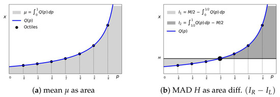
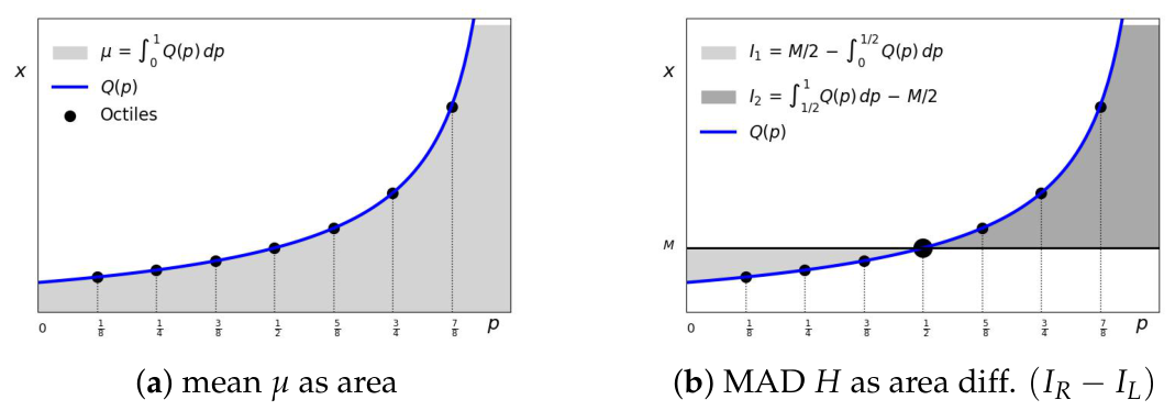
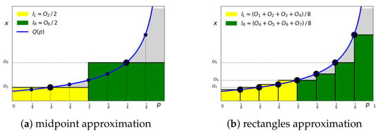
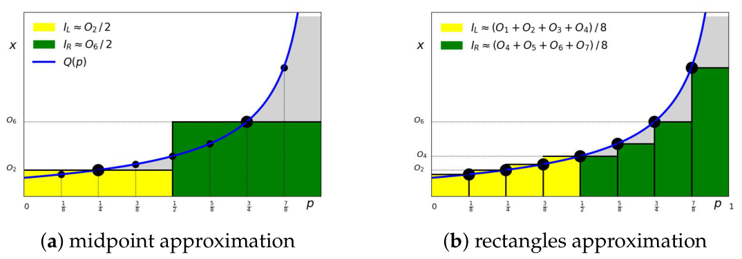
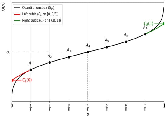
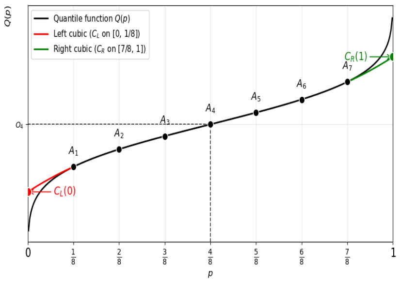
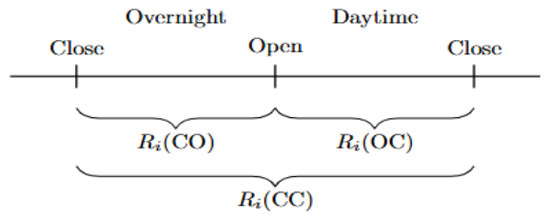
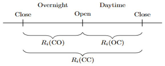
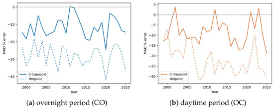
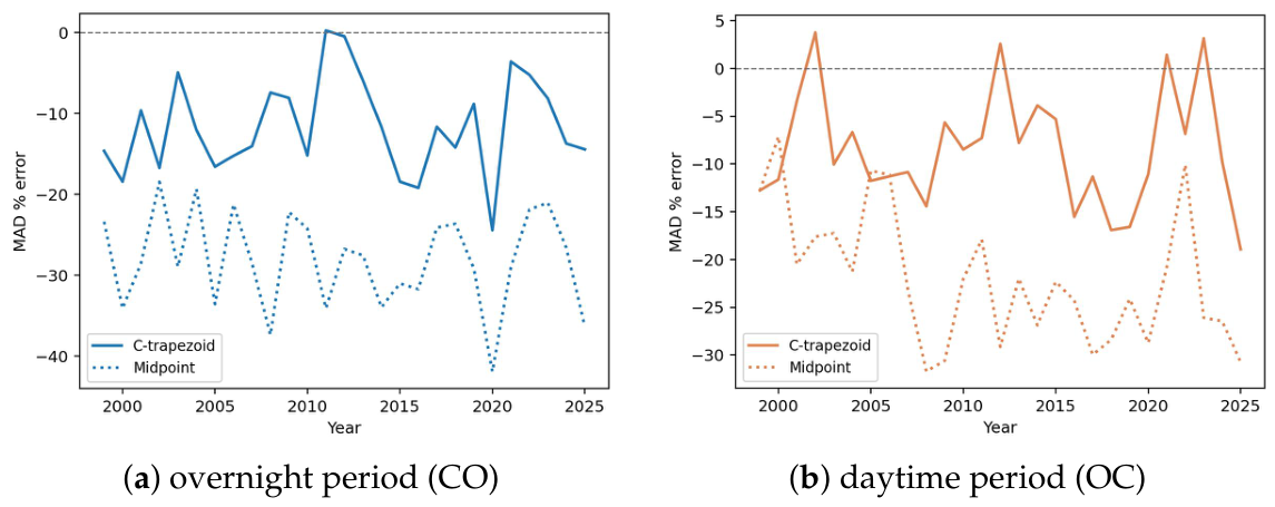
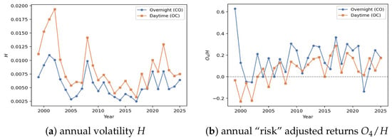
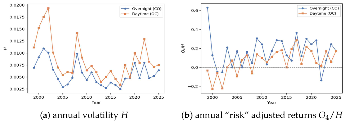
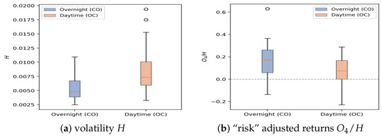
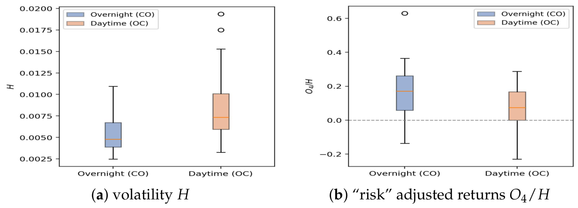
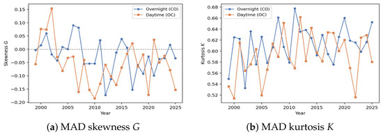
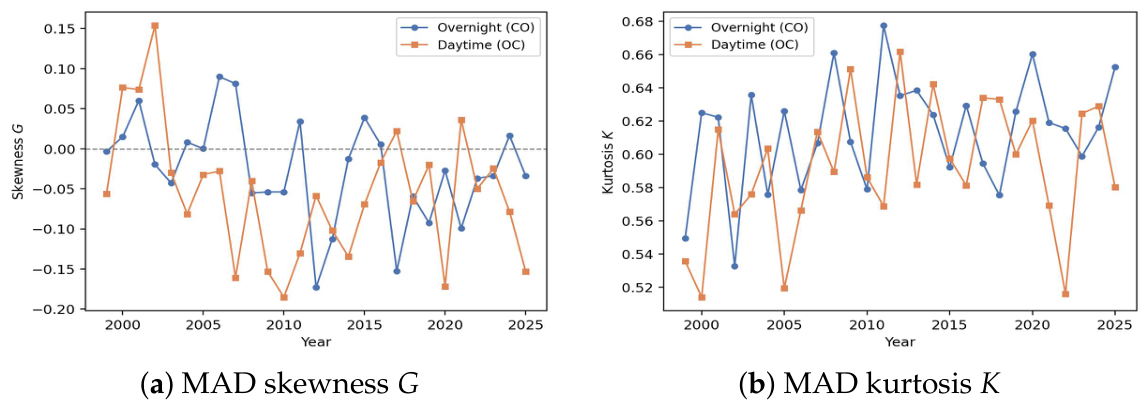
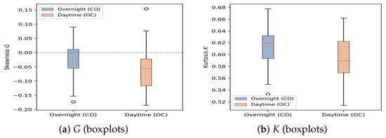
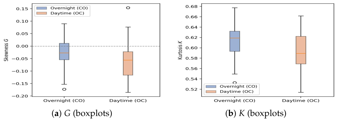
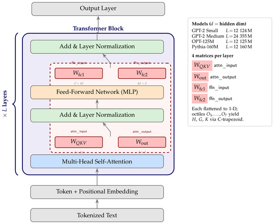
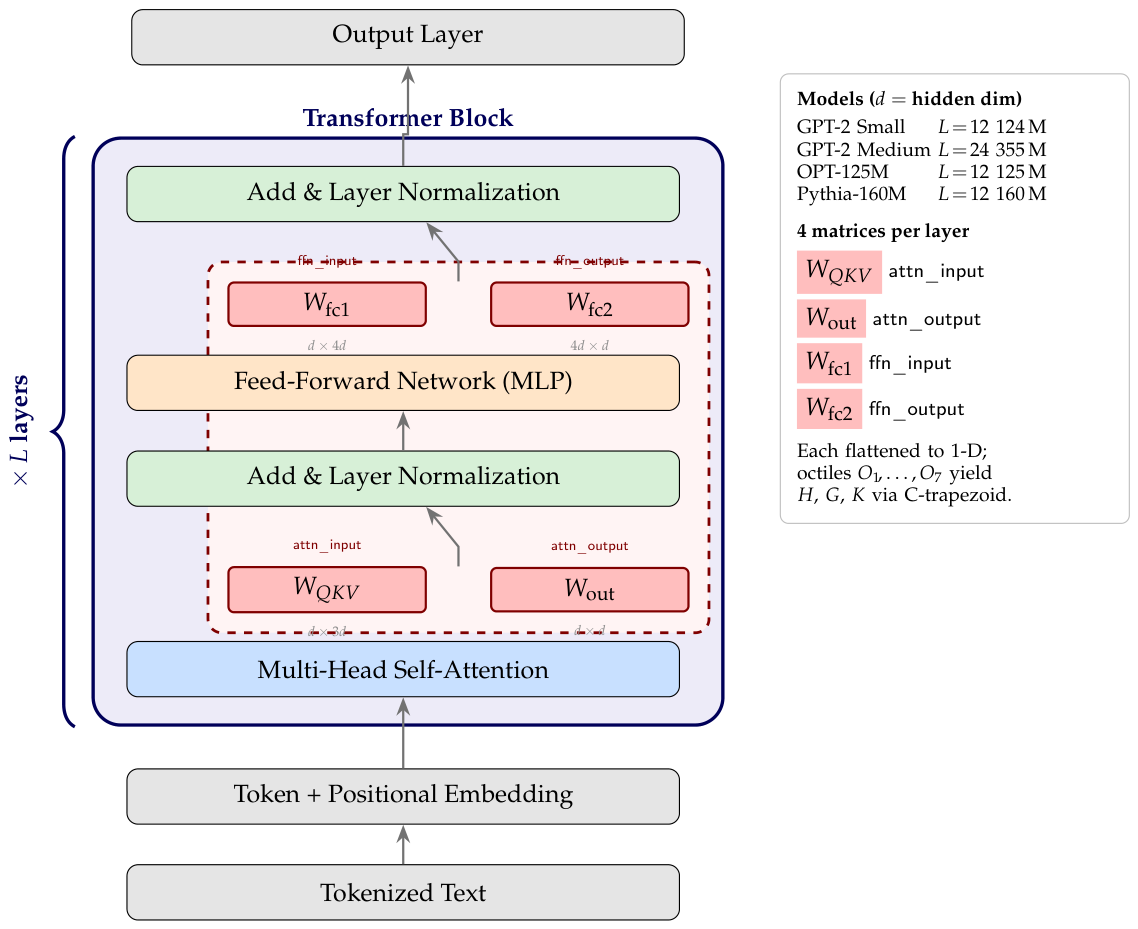
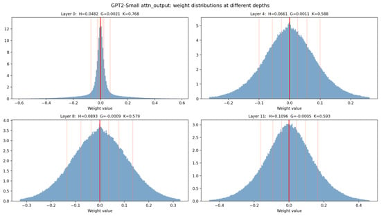
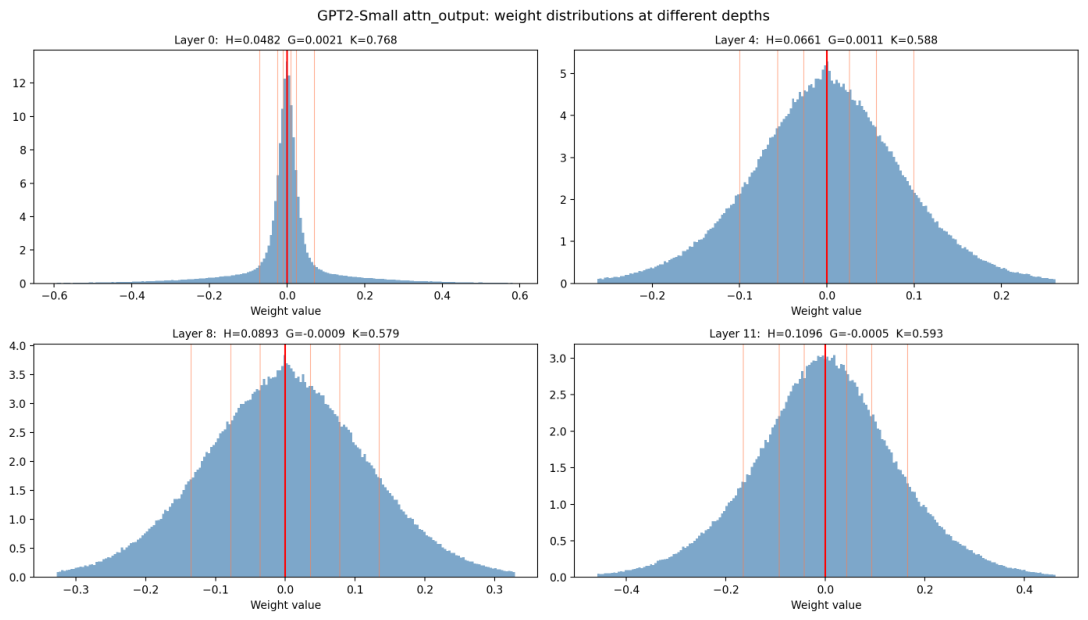
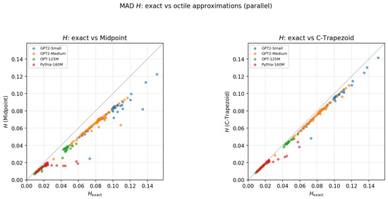
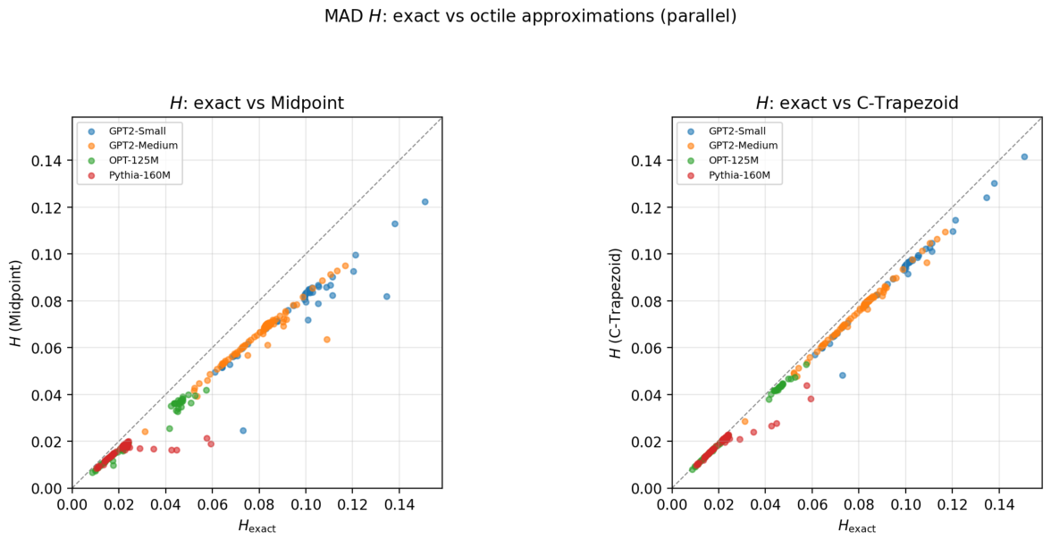
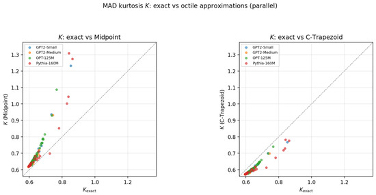
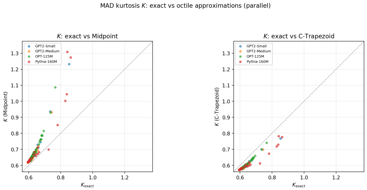
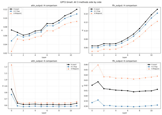
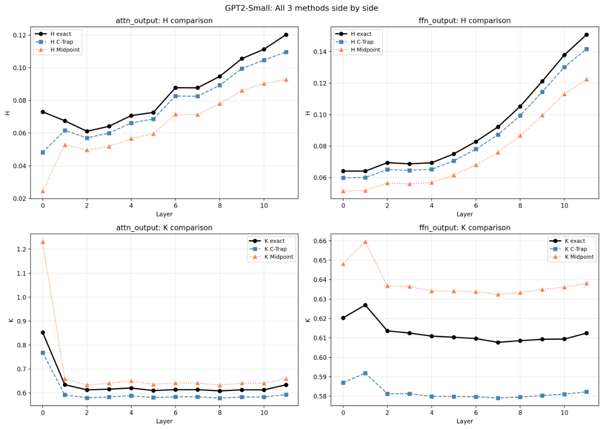
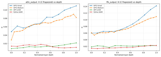
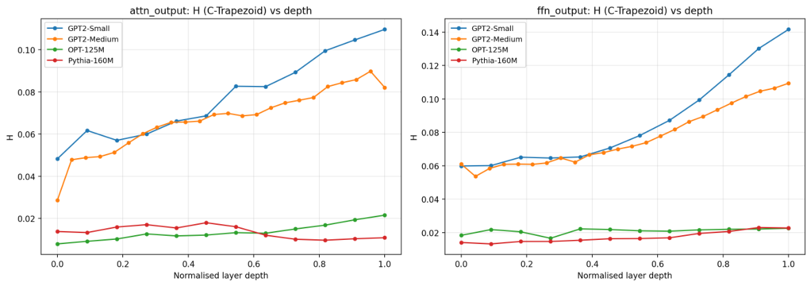
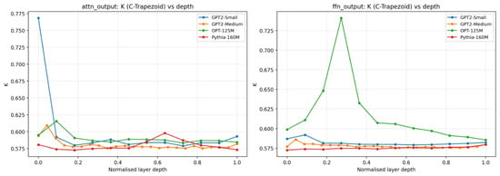
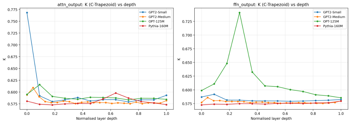
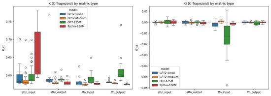
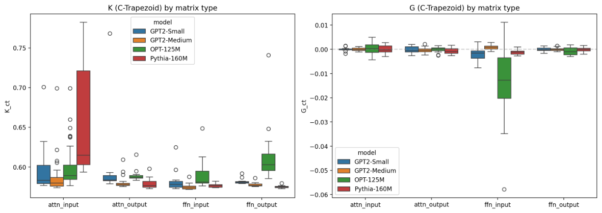
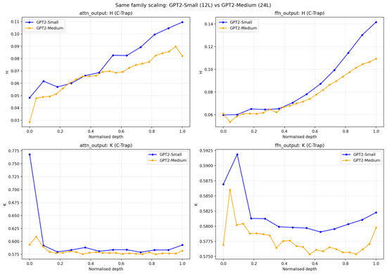
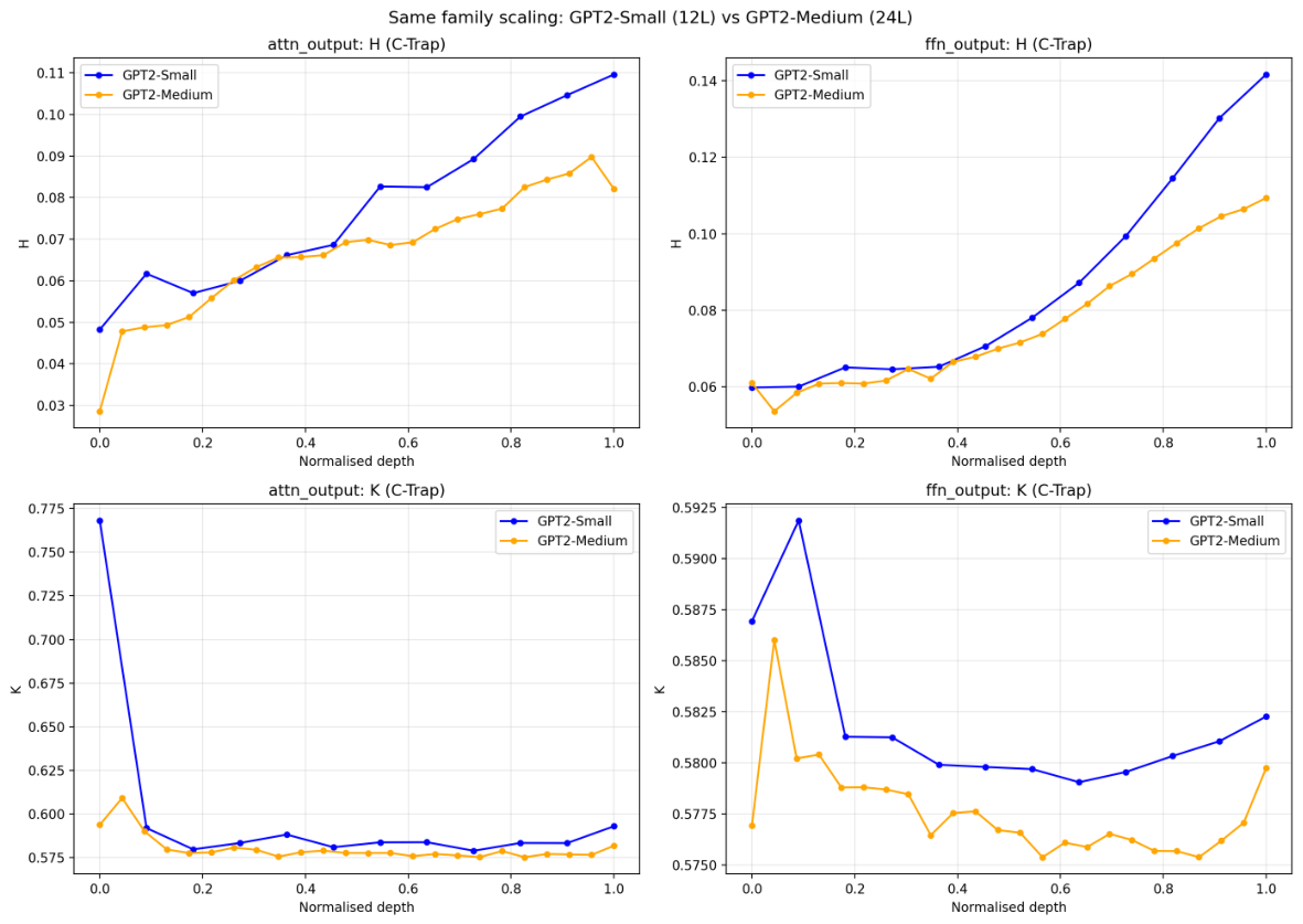
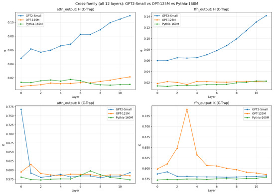
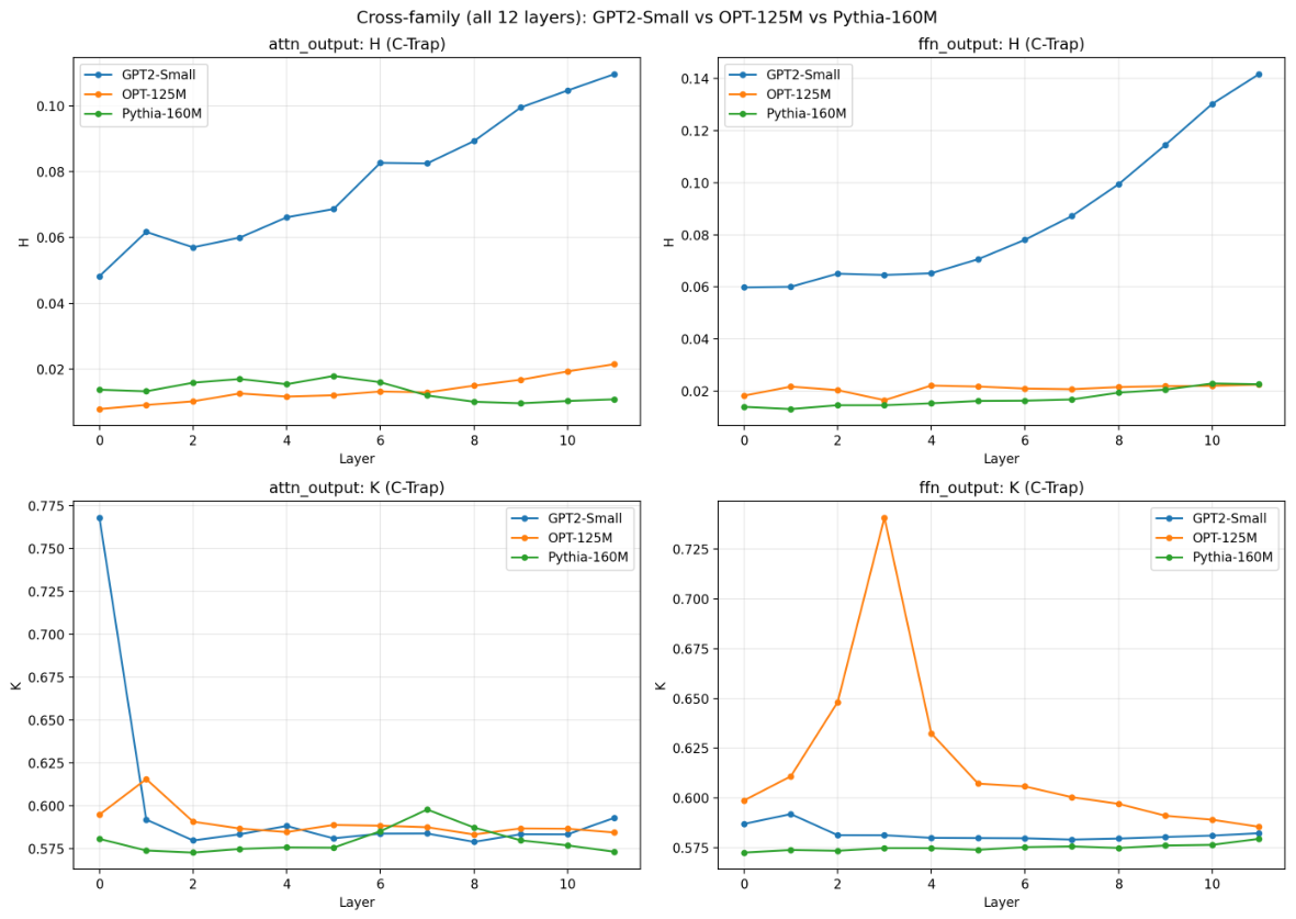

Disclaimer/Publisher’s Note: The statements, opinions and data contained in all publications are solely those of the individual author(s) and contributor(s) and not of MDPI and/or the editor(s). MDPI and/or the editor(s) disclaim responsibility for any injury to people or property resulting from any ideas, methods, instructions or products referred to in the content. |
© 2026 by the authors. Licensee MDPI, Basel, Switzerland. This article is an open access article distributed under the terms and conditions of the Creative Commons Attribution (CC BY) license.