Spacetime of Slowly Rotating Miyamoto–Nagai Source and Its Observability

Abstract

We construct a systematic general-relativistic model of the spacetime generated by a slowly rotating, axially symmetric, self-gravitating clump of collisionless matter whose gravitational potential is of Miyamoto–Nagai type. The metric is taken in a three-function cylindrical gauge, $d{s}^2=e^{a}d{t}^2-e^b(d{\rho }^2+d{z}^2)-{\rho }^2{e}^{c}d{\varphi }^2$, with the frame-dragging function $\omega$ added at the stationary level. We prove a no-go lemma of explicitly delimited scope (no pointwise relation $c=F(a,b)$ can annihilate the off-diagonal Ricci component) and reduce the field equations, for a diagonal source, to an algebraic system for $b_{\rho },b_z$ valid wherever ${(\nabla W)}^2\ne 0$, $W=\rho e^{(a+c)/2}$. The integrability of the resulting quadrature is not automatic: we prove that the compatibility condition ${\partial }_z{b}_{\rho }={\partial }_{\rho }{b}_z$ is exactly equivalent to the meridional matter-conservation equations—one combination of which is an identity, the other being the equation that determines the remaining metric function—and that at second order in $\beta =2GM/c^2$ it becomes the linear Poisson-type problem $\mathcal{L}{c}_2=4\kappa P_m$. A barotropy criterion shows that a prescribed flattened potential with strictly isotropic pressure is already inconsistent at the Newtonian level, whereas the Miyamoto–Nagai potential admits a globally physical anisotropic solution: density, meridional pressure and stress anisotropy follow in closed form, $\kappa P_m={\beta }^2{\epsilon }^2{(A+\zeta )}^2/\left(4{\zeta }^2{S}^3\right)$ and $\kappa (P_{\varphi }-P_m)=A{\beta }^2{\epsilon }^2{\rho }^2/\left(2{\zeta }^3{S}^3\right)$, all of definite sign, so that $P_{\varphi }>P_m$ everywhere off the axis and the anisotropy vanishes identically in the spherical limit. Rotation is included to Hartle order: the dragging obeys a linear equation at all orders in our gauge, the second-order diagonal metric is degenerate under the dispersion–rotation partition of the azimuthal support, and the degeneracy is broken only by the gravitomagnetic sector; the fully rotational realization gives $v_{\varphi }/v_c$ in closed form, which is near-circular for thin discs. On this basis we assess detectability: the flattening layer is routinely observable, with a deflection anisotropy decaying anomalously slowly (as $A/b$); galactic frame dragging (∼${10}^{-3}$μas ${\mathrm{yr}}^{-1}$) is astrometrically hopeless, but the parity-odd rotational asymmetry of time delays between opposite-side images of strongly lensed transients, $\mathsf{\Delta }t\sim 8GJ/c^{4}b\sim {10}^3$ s, is detectable in principle given VLBI-grade (∼10 μas) astrometry, the threshold being $M\gtrsim 2\times {10}^9{M}_{\odot }$ at disc-galaxy velocities; in the compact regime the model yields falsifiable energy-condition bounds (${\beta }_{\mathrm{DEC}}\approx 3.8\epsilon$, ${\beta }_{\mathrm{WEC}}\approx 6.8\epsilon$) and dragging frequencies in the QPO band.

1. Introduction

Potential–density pairs are the workhorse of galactic dynamics: closed-form potentials such as those of Plummer [1], Kuzmin [2] and Miyamoto–Nagai [3] underlie a large fraction of modeling of disks, bulges and halos [4]. Their general-relativistic status is less developed. Exact static and stationary axisymmetric frameworks are classical [5,6,7], and general-relativistic analogues of specific potential–density pairs have been constructed [8,9]; on the other hand, the theory of relativistic static fluid spheres is essentially complete [10,11,12,13,14], and rigidity theorems strongly constrain non-spherical static equilibria [15,16,17].

The present paper develops, from first principles, a general-relativistic model of the spacetime deformation produced by a finite, slowly rotating, axially symmetric “clump” of collisionless matter whose potential is prescribed to be of Miyamoto–Nagai type, and asks a question usually left implicit: which features of such a spacetime are observable in principle, and which are degenerate? Our contributions are:

• a compact form of the Ricci tensor in a three-function cylindrical gauge, and a no-go lemma of explicitly delimited scope—no local pointwise functional relation $c=F(a,b)$ between the metric functions can annihilate the off-diagonal component $R_{\rho z}$ identically (Section 2);
• a reduction of the field equations, for diagonal sources, to an algebraic system for the first derivatives of b together with one compatibility condition, and the proof—this is the logical core of the construction—that this compatibility condition is exactly equivalent to the meridional matter-conservation equations, reducing at second order to a single linear Poisson-type equation (Section 2.3 and Section 2.4);
• closed-form second-order density, meridional pressure and stress anisotropy for the Miyamoto–Nagai clump, all of definite sign, with the required azimuthal stress excess computed rather than postulated (Section 3);
• the slow-rotation extension—the frame dragging obeys a linear equation at all orders in our gauge, reducing at leading order to the axisymmetric Hartle equation, and the second-order diagonal metric is degenerate under the dispersion–rotation partition of the azimuthal support (Section 4);
• a layered assessment of detectability, including a parity-odd lensing-time-delay signature of the clump’s angular momentum, its scaling with the clump parameters, and falsifiable compactness bounds in the ultracompact regime (Section 5).

Throughout, subscripts on metric functions denote partial derivatives; the signature is $(+,-,-,-)$; $R_{\mu \nu }={\partial }_{\lambda }{\mathsf{\Gamma }}_{\mu \nu }^{\lambda }-{\partial }_{\nu }{\mathsf{\Gamma }}_{\mu \lambda }^{\lambda }+{\mathsf{\Gamma }}_{\lambda \sigma }^{\lambda }{\mathsf{\Gamma }}_{\mu \nu }^{\sigma }-{\mathsf{\Gamma }}_{\nu \sigma }^{\lambda }{\mathsf{\Gamma }}_{\mu \lambda }^{\sigma }$; the Hilbert–Einstein equations are used in the form $R_{\mu \nu }=\kappa (T_{\mu \nu }-\frac{1}{2}{g}_{\mu \nu }T)$ with $\kappa =8\pi G/c^4$; components of the Ricci tensor are listed in Appendix A; all symbolic results have been verified by computer algebra and all limits cross-checked numerically (Appendix B and Appendix C).

2. Framework

2.1. Metric, Ricci Tensor, Sources

We use dimensionless cylindrical coordinates $x^{\mu }=(t,\rho ,\varphi ,z)$ and the static ansatz

$$d{s}^2=e^{a(\rho ,z)}d{t}^2-e^{b(\rho ,z)}d{\rho }^2-{\rho }^2{e}^{c(\rho ,z)}d{\varphi }^2-e^{b(\rho ,z)}d{z}^2,$$

(1)

with $\sqrt{-g}=\rho e^{(a+2b+c)/2}$. The Ricci tensor has exactly five nonvanishing components, which are listed in Appendix A; we note here only that b enters $R_{tt}$ and $R_{\varphi \varphi }$ solely through $e^{-b}$, and that the off-diagonal component is

$$R_{\rho z}=-{\displaystyle \frac{1}{2}}\left[a_{\rho z}+c_{\rho z}+{\displaystyle \frac{a_{\rho }{a}_z}{2}}+{\displaystyle \frac{c_{\rho }{c}_z}{2}}-{\displaystyle \frac{b_z(a_{\rho }+c_{\rho })}{2}}-{\displaystyle \frac{b_{\rho }(a_z+c_z)}{2}}+{\displaystyle \frac{c_z-b_z}{\rho }}\right].$$

(2)

The source is taken to be

$${T^{\mu }}_{\nu }=\mathrm{diag}(D,-P_m,-P_{\varphi },-P_m),$$

(3)

where D is the energy density and $P_m$, $P_{\varphi }$ are meridional and azimuthal stresses.

• Physical setting and the meaning of the approximations.

Three modeling assumptions enter (3), and it is worth stating precisely what each does and does not claim.

(i) Collisionless matter in the mean-field approximation. The intended physical system is a galactic-scale clump—stars and dark matter—not a fluid star. For such systems the two-body relaxation time exceeds the Hubble time by many orders of magnitude, so the constituents move in the smooth self-consistent field rather than in a collision-dominated regime [4]. The correct kinetic description is then the Vlasov system [18] in the context of the General Relativity, whose stress tensor, after integration over momenta, has precisely the form (3): D is the energy density, and $P_m$, $P_{\varphi }$ are velocity-dispersion stresses, i.e., second moments of the distribution function, not thermodynamic pressures. No equation of state is assumed anywhere in this paper; the “pressures” are outputs of the geometry. We do not construct an explicit distribution function realizing the moments we obtain; this is the sense in which the model is mean-field, and it is stated again among the limitations in Section 5.6.

(ii) Static. “Static” at the level of Section 3 means that there is no mean bulk flow: all support against self-gravity is carried by velocity dispersion. This is a decomposition, not a physical restriction, because the same second-order geometry is produced by any partition of the azimuthal support between dispersion and rotation—exactly the degeneracy (32) that we exhibit in Section 4 and quantify in Section 5. Rotation is restored in Section 4, where the stationary sector is treated to Hartle order.

(iii) The compact member. The spherical, ultracompact configurations of Section 3.4 are the $A\to 0$ limit of the same anisotropic collisionless family, continued to $\beta /\epsilon =O\left(1\right)$. They are a mathematical limit of the construction and a testbed for energy-condition bounds; they are not offered as a model of a neutron star or of any collision-dominated compact object, for which the collisionless assumption would indeed be inappropriate.

The two structural conditions ${T^{\rho }}_z=0$ and $T_{\rho \rho }=T_{zz}$ hold exactly for (3), and these two drive the reduction below. They should be recognized as genuine restrictions on the matter, not as gauge choices: any two-dimensional metric can be brought to the conformal form $e^b(d{\rho }^2+d{z}^2)$ used in (1), so once that form is adopted the Einstein equations tie ${T^{\rho }}_z$ and ${T^{\rho }}_{\rho }-{T^z}_z$ to specific curvature combinations. The first condition, $⟨v_{\rho }{v}_z⟩=0$, states that the meridional velocity ellipsoid is aligned with the coordinate axes; the second, $⟨v_{\rho }^2⟩=⟨v_z^2⟩$, that it is round in that plane, $P_{\rho }=P_z\equiv P_m$. Real disc galaxies have ${\sigma }_R>{\sigma }_z$, so the second condition is an idealization; it is what closes the three-function ansatz, and we list it among the limitations in Section 5.6.

• On the word “isotropy”.

Because two distinct statements are easily conflated, we fix the terminology once. The ansatz (3) already imposes $P_{\rho }=P_z=P_m$: the velocity ellipsoid is assumed round in the meridional plane. We call this meridional isotropy; it is assumed. By strict isotropy we shall mean the further requirement $P_{\varphi }=P_m$, i.e., a fully round ellipsoid, which is what a perfect fluid would enforce; it is not assumed, and is shown below to be impossible for a flattened prescribed potential. For collisionless systems there is no mechanism enforcing it: the Jeans equations admit a free anisotropy function, and real galaxies are observed to be anisotropic, both in the disc velocity ellipsoid of the Milky Way [4] and in early-type systems mapped with integral-field spectroscopy [19]. Anisotropic static configurations in general relativity go back to [20,21] reviews the physics of local anisotropy in self-gravitating systems. The point of Section 3 is not that anisotropy is permitted but that for a flattened prescribed potential it is obligatory, and that its amount is computable in closed form rather than being a free function.

2.2. A No-Go Lemma: Statement and Scope

One might hope to eliminate one metric function by a pointwise relation $c=F(a,b)$ chosen so that $R_{\rho z}$ vanishes identically. This particular strategy is impossible:

Lemma 1. 

There is no $C^2$ function $F=F(a,b;\rho )$, defined pointwise on the values of the metric functions and possibly on ρ explicitly, such that substituting $c=F(a,b;\rho )$—together with the chain-rule expressions $c_{\rho }=F_a{a}_{\rho }+F_b{b}_{\rho }+F_{,\rho }$, $c_z=F_a{a}_z+F_b{b}_z$, $c_{\rho z}=F_a{a}_{\rho z}+F_b{b}_{\rho z}+\dots$—makes the right-hand side of (2) vanish identically as a polynomial in the jet variables $(a_{\rho },a_z,b_{\rho },b_z,a_{\rho z},b_{\rho z},\dots )$ regarded as independent.

Proof. 

Substituting and demanding identical vanishing, the coefficients of the independent jet variables $a_{\rho z}$, $b_{\rho z}$ and $a_{\rho }{a}_z$ give $1+F_a=0$, $F_b=0$ and $F_{aa}+\frac{1}{2}(1+F_a^2)=0$; the first forces $F_{aa}=0$, whence the third reads $1=0$.    □

Remark 1 

(scope). The Lemma is a statement about one reduction strategy and nothing more. It does not assert that the three metric functions are irreducible in general, and in particular it does not exclude: (i) relations involving derivatives of the metric functions, or differential constraints of higher order; (ii) the elimination of a or of b rather than c—the three functions are not on an equal footing in (1), and b in particular enters $R_{tt}$ and $R_{\varphi \varphi }$ only through the conformal factor $e^{-b}$; (iii) reductions valid on restricted classes of solutions rather than for arbitrary $a,b$; (iv) nonlocal or gauge-dependent reductions, for instance those following a change of the meridional chart. We draw from it only the negative conclusion that the naive pointwise elimination fails, and we therefore proceed by a different route, described next; that route does reduce the system, and its own scope is delimited in Section 2.3 and Section 2.4.

2.3. The Weyl-Type Reduction: What Is Prescribed and What Is Solved

Instead, $R_{\rho z}$ admits the covariant form $R_{\rho z}=-{\nabla }_{\rho }{\nabla }_z\alpha /\alpha -{\nabla }_{\rho }{\nabla }_z\gamma /\gamma$ with $\alpha =e^{a/2}$, $\gamma =\rho e^{c/2}$ and ∇ the covariant derivative of the 2-metric $e^b(d{\rho }^2+d{z}^2)$; equivalently, $R_{\rho z}=0$ is linear in $\gamma$. For the diagonal source (3) the two combinations $R_{\rho z}=\kappa T_{\rho z}=0$ and $R_{\rho \rho }-R_{zz}=\kappa (T_{\rho \rho }-T_{zz})=0$ are source-free, and with

$$\mathcal{P}\equiv a_{\rho }+c_{\rho }+{\displaystyle \frac{2}{\rho }}={\displaystyle \frac{2W_{\rho }}{W}},\mathcal{Q}\equiv a_z+c_z={\displaystyle \frac{2W_z}{W}},W\equiv \rho e^{(a+c)/2},$$

(4)

they form a linear algebraic system for the first derivatives of b,

$$b_z\mathcal{P}+b_{\rho }\mathcal{Q}=2S_1,b_{\rho }\mathcal{P}-b_z\mathcal{Q}=2S_2,$$

(5)

$$S_1=a_{\rho z}+c_{\rho z}+{\displaystyle \frac{a_{\rho }{a}_z}{2}}+{\displaystyle \frac{c_{\rho }{c}_z}{2}}+{\displaystyle \frac{c_z}{\rho }},S_2={\displaystyle \frac{a_{\rho \rho }-a_{zz}+c_{\rho \rho }-c_{zz}}{2}}+{\displaystyle \frac{a_{\rho }^2-a_z^2+c_{\rho }^2-c_z^2}{4}}+{\displaystyle \frac{c_{\rho }}{\rho }}.$$

(6)

The determinant of (5) is

$$-({\mathcal{P}}^2+{\mathcal{Q}}^2)=-{\displaystyle \frac{4{(\nabla W)}^2}{W^2}},{(\nabla W)}^2\equiv W_{\rho }^2+W_z^2,$$

(7)

so (5) determines $(b_{\rho },b_z)$ uniquely wherever ${(\nabla W)}^2\ne 0$; the degenerate set is discussed at the end of this subsection, and the integrability of the resulting quadrature is the subject of Section 2.4.

Two further identities complete the system. First, ${R^t}_t$ and ${R^{\varphi }}_{\varphi }$ depend on b only through the overall factor $e^{-b}$, and their sum is a total divergence of the flat meridional Laplacian ${\mathsf{\Delta }}_2\equiv {\partial }_{\rho }^2+{\partial }_z^2$,

$$\begin{array}{cc}\hfill {R^t}_t+{R^{\varphi }}_{\varphi }& =e^{-b}{\displaystyle \frac{{\mathsf{\Delta }}_{2}W}{W}}\hfill \\ \hfill ⟹{\mathsf{\Delta }}_{2}W& =-\kappa e^{b}W\left({T^{\rho }}_{\rho }+{T^z}_z\right)=2\kappa e^{b}W{P}_m.\hfill \end{array}$$

(8)

Second, the remaining components determine the matter, the inversion of ${R^{\mu }}_{\nu }=\kappa ({T^{\mu }}_{\nu }-\frac{1}{2}{{\delta }^{\mu }}_{\nu }T)$ for the anisotropic source (3) being

$$\begin{array}{cc}\hfill \kappa D& =\frac{1}{2}\left({R^0}_0-2{R^1}_1-{R^2}_2\right),\hfill \\ \hfill \kappa P_m& =\frac{1}{2}\left({R^0}_0+{R^2}_2\right)=\frac{1}{2}{e}^{-b}{\displaystyle \frac{{\mathsf{\Delta }}_{2}W}{W}},\hfill \\ \hfill \kappa (P_m-P_{\varphi })& ={R^2}_2-{R^1}_1,\hfill \end{array}$$

(9)

with ${R^3}_3={R^1}_1$ guaranteed by the second equation of (5). (For strictly isotropic sources, $P_{\varphi }=P_m$, the first two of (9) collapse to the more familiar $\kappa D=\frac{1}{2}({R^0}_0-3{R^1}_1)$ and $\kappa P_m=\frac{1}{2}({R^0}_0+{R^1}_1)$).

• What is prescribed and what is solved.

Equations (5)–(9) do not constitute a coupled Einstein–matter problem with an independently specified source. The logical order is:

(D1)

the potential a is prescribed—this is the model-building input, and the whole point of the potential–density-pair tradition;

(D2)

c is then determined by the compatibility condition of Section 2.4, which at $O\left({\beta }^2\right)$ becomes the linear Poisson-type Equation (17);

(D3)

b follows from (5) by quadrature, once (D2) guarantees that the quadrature exists;

(D4)

D, $P_m$ and $P_{\varphi }$ are then read off from (9); they are outputs, and their positivity and energy conditions are checks on the model, not inputs to it.

In particular, the statement that the problem reduces to “Weyl-type quadratures plus a linear Poisson-type problem” is a statement about this scheme at order ${\beta }^2$, and about nothing else. Equation (8) is linear in W only when $e^b$ and ${T^{\rho }}_{\rho }+{T^z}_z$ are regarded as already-known coefficients; in the exact problem they are not, and the system (5)–(9) is fully nonlinear. What makes the second-order scheme linear is (D1) together with the fact, established in Section 2.4, that at $O\left({\beta }^2\right)$ the source is fixed by a alone, so that (17) has a known right-hand side. We make no claim of linearity at higher order.

• The degenerate set ${(\nabla W)}^2=0$.

By (7), the algebraic solution of (5) fails exactly at critical points of W. Three remarks delimit this.

First, the condition ${(\nabla W)}^2\ne 0$ is not an artefact of our parametrization: it is precisely the classical condition under which W and its harmonic conjugate may be used as canonical Weyl coordinates [5,6], and its failure is the familiar breakdown of that chart, not of the field equations.

Second, at a point where $\nabla W=0$ one has $\mathcal{P}=\mathcal{Q}=0$, so (5) degenerates into the two conditions $S_1=S_2=0$ on $(a,c)$ alone, while $(b_{\rho },b_z)$ drop out of these two equations and are instead determined there by the remaining field equations, in particular by $R_{\rho \rho }+R_{zz}$, which contains $b_{\rho \rho }+b_{zz}$. The metric functions themselves and the Einstein equations remain perfectly regular; it is the solution formula, i.e., Cramer’s rule applied to (5), that degenerates.

Third, for the family actually constructed here, the degenerate set is empty. Since $W=\rho e^{(a+c)/2}$ we have $W_{\rho }=e^{(a+c)/2}(1+\rho u_{\rho })$ and $W_z=\rho e^{(a+c)/2}{u}_z$ with $u=(a+c)/2$; on the axis $\rho =0$ this gives $W_{\rho }=e^{(a+c)/2}\ne 0$, so the symmetry axis is never degenerate. Off the axis, with the second-order parametrization $a+c=c_2=O\left({\beta }^2\right)$ of Section 3,

$${(\nabla W)}^2=e^{c_2}\left[{\left(1+\frac{1}{2}\rho c_{2,\rho }\right)}^2+{\left(\frac{1}{2}\rho c_{2,z}\right)}^2\right]\ge e^{c_2}{\left(1-max|\frac{1}{2}\rho c_{2,\rho }|\right)}^2,$$

(10)

and the numerical solution of Section 3.3 gives $max|\frac{1}{2}\rho c_{2,\rho }| = 6.0 \times {10}^{-3}{\beta }^2$ for $A=\epsilon$, so that ${(\nabla W)}^2\ge {(1-0.006{\beta }^2)}^2>0$ everywhere for any $\beta \lesssim 1$. Finally, (8) shows that W is subharmonic in the meridional plane wherever $P_m\ge 0$, so it can have no interior maximum; this makes the appearance of critical points a non-generic possibility rather than the rule, though we do not attempt a general theorem here.

2.4. Integrability of the b-Quadratures

The system (5) yields $b_{\rho }$ and $b_z$ separately. A function b with these two derivatives exists on a simply connected domain if and only if the compatibility condition

$$\mathsf{\Xi }\equiv {\partial }_z{b}_{\rho }-{\partial }_{\rho }{b}_z=0$$

(11)

holds. This condition is not an identity in $(a,c)$: it is one additional third-order partial differential equation relating the two prescribed-and-sought metric functions, and it is exactly the equation referred to as (D2) above. Its content is the following.

Proposition 1 

(compatibility = matter conservation). Let $\mathcal{D}\subset \{\rho >0\}$ be simply connected, let $a,c\in C^3\left(\mathcal{D}\right)$ with ${(\nabla W)}^2\ne 0$ on $\mathcal{D}$, let $(b_{\rho },b_z)$ be the unique solution of (5), and let $D,P_m,P_{\varphi }$ be defined by (9). Then, identically on $\mathcal{D}$,

$$\kappa e^b{\nabla }_{\mu }{T^{\mu }}_z=+{\displaystyle \frac{W_{\rho }}{2W}}\mathsf{\Xi },\kappa e^b{\nabla }_{\mu }{T^{\mu }}_{\rho }=-{\displaystyle \frac{W_z}{2W}}\mathsf{\Xi }.$$

(12)

Equivalently,

$$W_{\rho }{\nabla }_{\mu }{T^{\mu }}_{\rho }+W_z{\nabla }_{\mu }{T^{\mu }}_z\equiv 0,W_{\rho }{\nabla }_{\mu }{T^{\mu }}_z-W_z{\nabla }_{\mu }{T^{\mu }}_{\rho }=+{\displaystyle \frac{{(\nabla W)}^2}{2\kappa W{e}^b}}\mathsf{\Xi }.$$

(13)

Consequently, $\mathsf{\Xi }=0$ if and only if ${\nabla }_{\mu }{T^{\mu }}_{\rho }={\nabla }_{\mu }{T^{\mu }}_z=0$, i.e., if and only if the source read off from the geometry is in hydrostatic equilibrium.

The identity (12) is proved in Appendix B: once the two source-free equations are put in normal form, it is a short consequence of the contracted Bianchi identity together with the observation that the reduction replaces a holonomic 2-jet of b by a non-holonomic one, the defect being exactly $\mathsf{\Xi }$. An independent, unsampled computer-algebra verification on arbitrary $a(\rho ,z)$, $c(\rho ,z)$ accompanies it as Supplementary Material. Three consequences answer the questions that motivate the Proposition.

(1) The compatibility condition is not automatic, and it is not an extra assumption either. One combination of the two conservation equations, the first of (13), holds identically once (5) is imposed—this is the Bianchi content of the reduction. The orthogonal combination is the integrability condition. Thus (11) is precisely as strong as demanding that the matter satisfy ${\nabla }_{\mu }{T}^{\mu \nu }=0$, which any solution of the Einstein equations must; but it constrains $(a,c)$ and must be solved, not assumed.

(2) At $O\left({\beta }^2\right)$ it is the linear Poisson-type problem. Writing $a=O\left(\beta \right)$, $b=-a+b_2$, $c=-a+c_2$ with $b_2,c_2=O\left({\beta }^2\right)$, the system (5) gives the two quadratures

$$b_{2,z}=c_{2,z}+\rho c_{2,\rho z}+\rho a_{\rho }{a}_z,b_{2,\rho }=c_{2,\rho }+{\displaystyle \frac{\rho }{2}}\left(c_{2,\rho \rho }-c_{2,zz}\right)+{\displaystyle \frac{\rho }{2}}\left(a_{\rho }^2-a_z^2\right),$$

(14)

whose compatibility defect is, exactly,

$$\mathsf{\Xi }=-{\displaystyle \frac{\rho }{2}}\left[{\partial }_z\left(\mathcal{L}{c}_2\right)+2a_z\mathsf{\Delta }a\right]+O\left({\beta }^3\right),\mathcal{L}={\partial }_{\rho }^2+{\displaystyle \frac{2}{\rho }}{\partial }_{\rho }+{\partial }_z^2={\displaystyle \frac{1}{\rho }}{\mathsf{\Delta }}_2(\rho ·),$$

(15)

with $\mathsf{\Delta }={\partial }_{\rho }^2+{\rho }^{-1}{\partial }_{\rho }+{\partial }_z^2$. Since $\kappa D=\mathsf{\Delta }a+O\left({\beta }^2\right)$ and, by (8), $\kappa P_m=\frac{1}{4}\mathcal{L}{c}_2+O\left({\beta }^3\right)$, the vanishing of (15) reads

$${\partial }_z\left(\kappa P_m\right)=-\frac{1}{2}\kappa D{a}_z,$$

(16)

which is the z-component of hydrostatic equilibrium. Integrating (16) in z with $P_m\to 0$ at infinity determines $P_m$ from a alone, and $c_2$ then follows from

$$\mathcal{L}{c}_2=4\kappa P_m,$$

(17)

a linear elliptic problem with a known right-hand side and a unique decaying solution. This is the precise sense of the phrase “Weyl-type quadratures plus a linear Poisson-type problem”.

(3) The ρ-component fixes the anisotropy. The remaining conservation equation, ${\nabla }_{\mu }{T^{\mu }}_{\rho }=0$, reads at this order

$$\begin{array}{cc}\hfill {\partial }_{\rho }\left(\kappa P_m\right)+\frac{1}{2}\kappa D{a}_{\rho }+{\displaystyle \frac{\kappa (P_m-P_{\varphi })}{\rho }}& =0\hfill \\ \hfill ⟹\kappa (P_m-P_{\varphi })& =-\rho \left[{\partial }_{\rho }\left(\kappa P_m\right)+\frac{1}{2}\kappa D{a}_{\rho }\right]+O\left({\beta }^3\right),\hfill \end{array}$$

(18)

so that the azimuthal stress anisotropy is not an independent function at all: it is determined in closed form by the prescribed potential. Equation (18) is equivalent to (26) below, but is far more convenient, since it involves only a and $P_m$ and no derivatives of $c_2$; the equivalence is verified symbolically in Appendix B.

3. The Static Miyamoto–Nagai Clump

3.1. Why Not a “Flattened Plummer” Potential: A Barotropy Criterion

Suppose the potential is prescribed, $e^a$ given, and the pressure is required to be strictly isotropic ($P_{\varphi }=P_m=P$). Counting shows the system is then overdetermined by one condition. The obstruction is physical: hydrostatic equilibrium $P_{,i}=-\frac{1}{2}(D+P)a_{,i}$ (a Bianchi consequence, and the isotropic specialization of (16)–(18)) forces the level surfaces of D and a to coincide, so a necessary condition is the vanishing of the barotropy Jacobian

$$J\equiv a_{\rho }{\left(\mathsf{\Delta }a\right)}_z-a_z{\left(\mathsf{\Delta }a\right)}_{\rho },\mathsf{\Delta }\equiv {\partial }_{\rho }^2+{\rho }^{-1}{\partial }_{\rho }+{\partial }_z^2.$$

(19)

For the naive flattened Plummer potential $a=-\beta {({\rho }^2+k^2{z}^2+{\epsilon }^2)}^{-1/2}$ one finds $J\ne 0$ whenever $k\ne 1$; moreover its Newtonian density $\kappa D=\mathsf{\Delta }a$ changes sign far from the source. Both defects have one root: the equipotentials keep a fixed eccentricity out to infinity, which no bounded positive source can produce. This is the practical face of the classical sphericity theorems [15,16,17].

3.2. The Miyamoto–Nagai Potential: Closed-Form Source

The minimal repair is the Miyamoto–Nagai potential [3],

$$a=-{\displaystyle \frac{\beta }{\sqrt{S}}},S={\rho }^2+{(A+\zeta )}^2,\zeta =\sqrt{z^2+{\epsilon }^2},$$

(20)

which flattens by the vertical shift $A+\zeta$ (Kuzmin’s image construction [2]), interpolates between the Plummer sphere ($A\to 0$) and the Kuzmin disk ($\epsilon \to 0$), and has direct parameters: A the radial scale, $\epsilon$ the thickness, $\beta =2GM/c^2$ (in units of the length scale). With $b=-a+b_2$, $c=-a+c_2$ the construction of Section 2.4 gives, in closed form,

$$\begin{array}{cc}\hfill \kappa D& =\mathsf{\Delta }a+O\left({\beta }^2\right)={\displaystyle \frac{\beta {\epsilon }^2\left[A{\rho }^2+(A+3\zeta ){(A+\zeta )}^2\right]}{S^{5/2}{\zeta }^3}},\hfill \end{array}$$

(21)

$$\begin{array}{cc}\hfill \kappa P_m& ={\displaystyle \frac{{\beta }^2{\epsilon }^2{(A+\zeta )}^2}{4{\zeta }^2{S}^3}}+O\left({\beta }^3\right),\hfill \end{array}$$

(22)

$$\begin{array}{cc}\hfill \kappa (P_{\varphi }-P_m)& ={\displaystyle \frac{A{\beta }^2{\epsilon }^2{\rho }^2}{2{\zeta }^3{S}^3}}+O\left({\beta }^3\right),\hfill \end{array}$$

(23)

all three manifestly of definite sign. Equation (22) follows by integrating (16), the hydrostatic integral becoming rational under $zdz=\zeta d\zeta$ with its denominator collapsing to $S^3$; Equation (23) then follows from (18) by differentiation alone, the bracket collapsing as $-3\zeta {(A+\zeta )}^2+A{\rho }^2+(A+3\zeta ){(A+\zeta )}^2=A\left[{(A+\zeta )}^2+{\rho }^2\right]=AS$. At $A=0$ Equations (21) and (22) reproduce the Plummer sphere, for which (22) is exactly the $n=5$ polytropic relation $P\propto D^{6/5}$ [1,22], and (23) vanishes identically, as it must.

Three consequences are worth isolating. First, the sign in (23) is unconditional: for $A>0$ and $\rho >0$ one has $P_{\varphi }>P_m$ everywhere, so the flattening is supported by an azimuthal stress excess throughout the configuration, as tensor-virial intuition suggests. Second, the relative anisotropy is elementary,

$${\displaystyle \frac{P_{\varphi }-P_m}{P_m}}={\displaystyle \frac{2A{\rho }^2}{\zeta {(A+\zeta )}^2}},$$

(24)

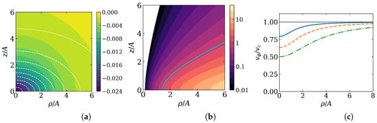
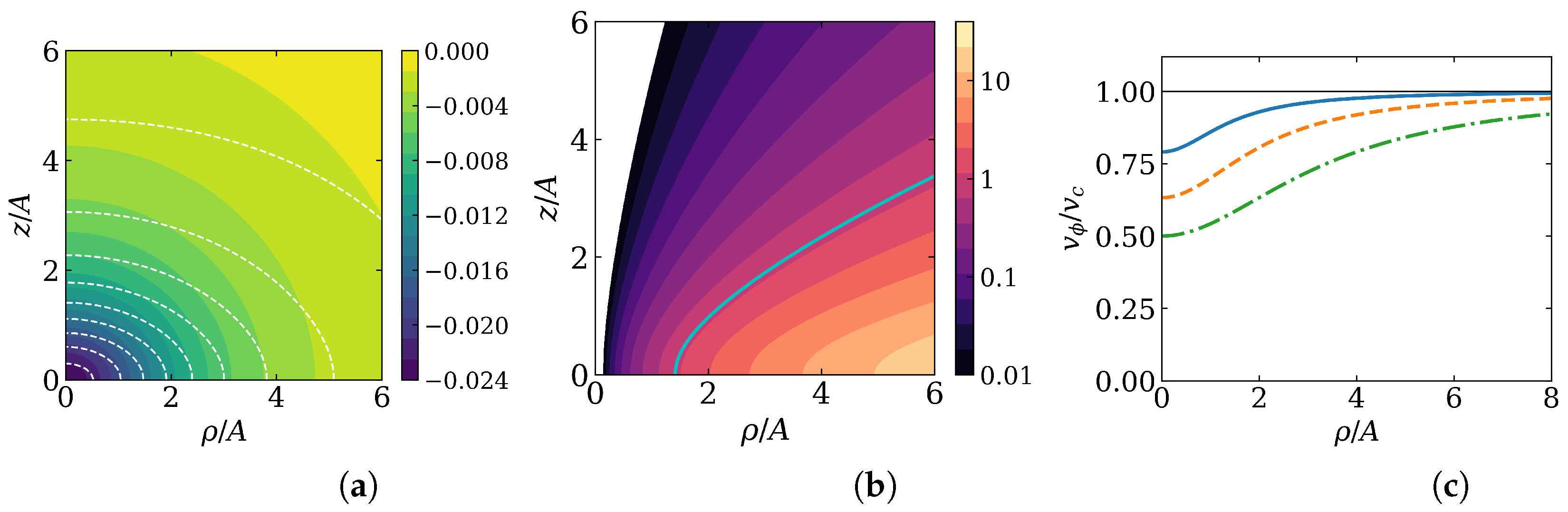
vanishing on the axis and growing outwards in the plane (Figure 1b). Third, in the fully rotational realization—strictly isotropic dispersions, all the azimuthal excess carried by streaming, $D{v}_{\varphi }^2=P_{\varphi }-P_m$ (Section 4)—the required rotation is also closed-form,

$${\displaystyle \frac{v_{\varphi }^2}{v_c^2}}={\displaystyle \frac{AS}{A{\rho }^2+(A+3\zeta ){(A+\zeta )}^2}},v_c^2=\frac{1}{2}\rho a_{\rho },$$

(25)

which is ≤1 throughout, tends to 1 as $\rho \to \infty$ in the midplane, and equals $A/(A+3\epsilon )$ at the center. For a round clump, $\epsilon =A$, the midplane value is $({\rho }^2+4A^2)/({\rho }^2+16A^2)$, i.e., $v_{\varphi }\simeq (0.54$–$0.84)v_c$ for $\rho =(1$–$5)A$; for a thin disc, $\epsilon =0.2A$, the same range gives $v_{\varphi }\simeq (0.86$–$0.98)v_c$ (Figure 1c). The trend is the physically expected one: thin, flattened configurations are nearly rotationally supported, round ones are dispersion-dominated, and the model quantifies the crossover without any free parameter.

Figure 1. Second-order structure of the Miyamoto–Nagai clump, for $A=\epsilon$. (a) Numerical solution of (17) for $c_2$ (filled contours, color scale at right, in units of ${\beta }^2$) together with $b_2$ from the quadratures (14) (white dashed contours); horizontal axis $\rho /A$, vertical axis $z/A$. (b) The closed-form relative stress anisotropy (24), $(P_{\varphi }-P_m)/P_m=2A{\rho }^2/\left[\zeta {(A+\zeta )}^2\right]$, on a logarithmic color scale; the cyan curve marks $P_{\varphi }-P_m=P_m$; axes as in (a). (c) The fully rotational realization (25) in the midplane, $v_{\varphi }/v_c$ against $\rho /A$; the solid, dashed and dash-dotted curves are $\epsilon /A=0.2$, $0.5$ and 1 respectively, and the thin horizontal line marks $v_{\varphi }=v_c$. Thin discs are nearly rotationally supported, round clumps are dispersion-dominated.

The residual metric functions obey (17) and the quadratures (14), which are a linear Poisson-type problem with unique decaying solution—elementary for $A=0$, where $b_2=c_2=-a^2/8$, and not elementary for $A>0$. For completeness we record the equivalent form of the anisotropy in terms of the metric functions,

$$\kappa (P_m-P_{\varphi })=-{\displaystyle \frac{1}{2}}\left[b_{2,\rho \rho }+b_{2,zz}-c_{2,zz}+a_{\rho }^2-{\displaystyle \frac{b_{2,\rho }}{\rho }}\right]+O\left({\beta }^3\right),$$

(26)

which reduces to (18), and hence to (23), upon substituting (14) and (17). Since $J\ne 0$ for $A>0$, some anisotropy (or rotation, Section 4) is obligatory—and (23) states exactly how much.

3.3. Numerical Solution for the Second-Order Metric Functions

The matter content at $O\left({\beta }^2\right)$ is closed-form, by (21)–(23); what still requires numerical work is the pair of metric functions $c_2$ and $b_2$ themselves, which enter the post-Newtonian diagonal observables of Section 5.2 and the regularity checks below.

• Scheme.

Equation (17) is solved in the variable $\psi \equiv \rho c_2$, for which $\mathcal{L}{c}_2={\rho }^{-1}{\mathsf{\Delta }}_2\psi$ and the problem becomes the flat two-dimensional Poisson equation

$${\mathsf{\Delta }}_2\psi =4\rho \kappa P_m,$$

(27)

on the quadrant $[0,R_{max}]\times [0,R_{max}]$ with $R_{max}=60A$, discretized on a uniform grid of $n^2$ points with the standard second-order five-point Laplacian [23], $h=R_{max}/(n-1)$. The boundary conditions are: $\psi =0$ on the axis $\rho =0$ (regularity, since $c_2$ is bounded there); the reflection symmetry $c_2(\rho ,-z)=c_2(\rho ,z)$ at $z=0$, implemented by mirroring the stencil; and Dirichlet data on the two outer edges taken from the monopole asymptotics. The latter is fixed as follows: $\mathcal{L}$ is the flat Laplacian of ${\mathbb{R}}^3\oplus \mathbb{R}$ acting on functions of $(\rho ,z)$ alone, its decaying radial solution is $c_2\to C/r^2$ with $r^2={\rho }^2+z^2$, and matching to the source gives

$$C=-{\displaystyle \frac{1}{\pi }}{\int }_{\rho >0}4\kappa P_m{\rho }^{2}d\rho dz.$$

(28)

For $A=0$ this evaluates to $C=-{\beta }^2/8$, reproducing the exact solution $c_2=-a^2/8$; for $A=\epsilon$ it gives $C=-0.07135{\beta }^2$. The resulting sparse linear system is solved by a direct (LU) method. $b_2$ is then obtained from (14) by trapezoidal quadrature, integrating inwards from the far corner where $b_2\to 0$.

• Validation and convergence.

Table 1 collects the three diagnostics. The first is the exact spherical solution $c_2=-a^2/8$ at $A=0$, reproduced with a maximum relative error inside $r\le 10\epsilon$ that falls by a factor of about four per grid halving, i.e., at the expected second order, reaching $0.49\%$ on ${601}^2$. The second is elementary flatness on the axis: $b_2=c_2$ at $\rho =0$ is not imposed anywhere in the scheme—it emerges, at the $8\times {10}^{-5}{\beta }^2$ level on ${601}^2$, as a nontrivial check on the whole chain (Poisson solve, quadrature and boundary treatment together). The third is the central value $c_2(0,0)$, stable at $-0.0235{\beta }^2$ for $A=\epsilon =1$. Finally, evaluating the metric-space form (26) on the numerical solution reproduces the closed form (23) at the $23\%$, $18\%$ and $15\%$ rms level on ${301}^2$, ${601}^2$ and ${901}^2$; the slow convergence is entirely expected, since (26) requires third differences of a quadrature of a numerical solution, and it is precisely why the closed form (18)—which is exact—is used for all physical statements. The thin-disk case $\epsilon =0.2A$ behaves identically at the sign level but calls for adaptive resolution for precision work on $c_2$ itself.

Table 1. Convergence of the solution of (27). Column 3: maximum relative error inside $r\le 10\epsilon$ against the exact spherical solution $c_2=-a^2/8$. Column 4: the emergent (not imposed) elementary-flatness residual on the axis. Column 5: central value for $A=\epsilon$.

n	$\mathit{h}/\mathit{A}$	Max Rel. Error vs. Exact ($\mathit{A}=0$)	$|{\mathit{b}}_2-{\mathit{c}}_2{|}_{\mathit{\rho }=0}$ ($\mathit{A}=\mathit{\epsilon }$)	${\mathit{c}}_2(0,0)/{\mathit{\beta }}^2$
151	$0.400$	$5.4\%$	$5.4\times {10}^{-4}$	$-0.02398$
301	$0.200$	$1.8\%$	$2.3\times {10}^{-4}$	$-0.02366$
601	$0.100$	$0.49\%$	$7.9\times {10}^{-5}$	$-0.02355$

3.4. The Spherical Member and Its Compactness Bounds

For $A=0$ the configuration is spherical and can be followed into the relativistic regime: with $b=c=f\left(r\right)$ all constraints collapse to one ODE, linearized by $w=e^{-f/2}$,

$$w^{″}-\left(a^{\prime }+{\displaystyle \frac{1}{r}}\right)w^{\prime }-{\displaystyle \frac{1}{2}}\left(a^{″}+{\displaystyle \frac{a^{\prime 2}}{2}}-{\displaystyle \frac{a^{\prime }}{r}}\right)w=0,$$

(29)

paralleling known generating techniques [10,12,13,14]. The regular, asymptotically flat solution exists and is unique; its two tails carry the same mass, $M_f=M_a=\beta /2$, so the exterior is Schwarzschild-like. Numerically, the dominant energy condition at the center holds for $\beta \lesssim 3.8\epsilon$ ($GM/c^2\epsilon \lesssim 1.9$) and the weak energy condition for $\beta \lesssim 6.8\epsilon$; these Buchdahl-type boundaries [11] delimit the horizonless ultracompact (“mimicker”) regime [24].

4. Slow Rotation

Stationarity is included by $dt\to dt-\omega (\rho ,z)d\varphi$ in (1) (the Lewis–Papapetrou class, same W). For purely azimuthal flow the circularity conditions hold, and two exact facts make rotation inexpensive. First, the Weyl-type combinations acquire only explicit additions,

$$R_{\rho z}\to R_{\rho z}^{\mathrm{stat}}+{\displaystyle \frac{e^{a-c}}{2{\rho }^2}}{\omega }_{\rho }{\omega }_z,R_{\rho \rho }-R_{zz}\to {(·)}^{\mathrm{stat}}+{\displaystyle \frac{e^{a-c}}{2{\rho }^2}}({\omega }_{\rho }^2-{\omega }_z^2),$$

(30)

so the quadratures survive, with $S_1,S_2$ of (6) shifted by these explicit $\omega$-terms; since $\omega =O\left({\beta }^{3/2}\right)$ the additions are $O\left({\beta }^3\right)$ and therefore do not affect the compatibility analysis of Section 2.4 at the order retained here. Second, the $\left(t\varphi \right)$ equation is governed by the identity

$${R^{\varphi }}_t={\displaystyle \frac{e^{-b}}{2W}}\left[{\partial }_{\rho }\left({\displaystyle \frac{e^{2a}{\omega }_{\rho }}{W}}\right)+{\partial }_z\left({\displaystyle \frac{e^{2a}{\omega }_z}{W}}\right)\right]⟹\nabla ·\left({\displaystyle \frac{e^{2a}}{W}}\nabla \omega \right)=2\kappa W{e}^b{T^{\varphi }}_t,$$

(31)

linear in $\omega$ at all orders. For virialized motion $v\sim c\sqrt{\beta }$ one has $\omega =O\left({\beta }^{3/2}\right)$ and back-reaction $O\left({\beta }^3\right)$: the $O\left({\beta }^2\right)$ diagonal sector of Section 3 is unchanged, rotation entering only through

$${T^{\varphi }}_{\varphi }=-\left(P_{\varphi }^{\mathrm{disp}}+D{v}_{\varphi }^2\right)+O\left({\beta }^3\right),v_{\varphi }=\rho \mathsf{\Omega },$$

(32)

the familiar dispersion–rotation degeneracy [4]; Equation (25) is the extreme member of this family, with $P_{\varphi }^{\mathrm{disp}}=P_m$. At leading order, with $\tilde{\omega }=\omega /{\rho }^2$ the dragging rate,

$${\tilde{\omega }}_{\rho \rho }+{\displaystyle \frac{3}{\rho }}{\tilde{\omega }}_{\rho }+{\tilde{\omega }}_{zz}=2\kappa D\mathsf{\Omega }$$

(33)

—the axisymmetric form of the Hartle slow-rotation equation [25,26], with $\tilde{\omega }\to 2G\tilde{J}/c^2{r}^3$ defining the angular momentum $\tilde{J}$. The Hartle expansion is an expansion in $\mathsf{\Omega }/{\mathsf{\Omega }}_{\mathrm{K}}$; comparisons with fully numerical stationary spacetimes show that it remains accurate at the percent level well beyond the formally slow-rotation regime [27], which is far more than we need at $\beta \sim {10}^{-6}$. Pure rotation with isotropic dispersions would require, by the Poincaré–Wavre property of barotropic equilibrium figures [28,29], that $Q\equiv (D_z{\mathsf{\Phi }}_{\rho }-D_{\rho }{\mathsf{\Phi }}_z)/\left(\rho D_z\right)$ ($\mathsf{\Phi }=a/2$) be independent of z; numerically this fails for (20) (e.g., Q drops thirtyfold between $z=0.2$ and $z=2$ at $\rho =0.5$ for $A=1$, $\epsilon =0.2$), so the generic support is a dispersion–rotation mix, with the Q-map showing where rotation may dominate. At the exact nonlinear level the $(a,\omega )$ sector becomes Ernst-type and is integrable only in vacuum [30]; the Hartle order suffices for $\beta \ll 1$.

5. Observability: What Is Measurable in Principle

The construction organizes the observables into three layers with sharply different accessibility. We quote numbers for a Milky-Way-like clump; the choice of this fiducial, and the scaling away from it, are discussed in Section 5.4. The adopted values are a disc-plus-bulge mass $M\simeq 6\times {10}^{10}{M}_{\odot }$, a circular speed $v\simeq 220$ km ${\mathrm{s}}^{-1}$ and a radial scale $\simeq 5$ kpc, consistent with the Milky Way parameters compiled in [31] and with the mass models and rotation-curve determinations of [32,33]; the Galactocentric distance $R_0=8.178\pm 0.026$ kpc is taken from [34]. These give $J\sim MvR\simeq 4\times {10}^{66}$ kg ${\mathrm{m}}^2$ ${\mathrm{s}}^{-1}$ and, with $\beta =2GM/c^2$ expressed in units of the radial scale,

$$\beta ={\displaystyle \frac{2GM}{c^2\times 5\mathrm{kpc}}}={\displaystyle \frac{5.7\times {10}^{-3}\mathrm{pc}}{5\times {10}^3\mathrm{pc}}}\simeq 1.1\times {10}^{-6},$$

(34)

whence the $\beta \sim {10}^{-6}$ used throughout. For the ultracompact regime $\beta /\epsilon \sim O\left(1\right)$.

5.1. The Newtonian Layer, $O\left(\beta \right)$: Flattening

The potential (20) itself—rotation curves, vertical kinematics, and the quadrupole structure of lensing—is routinely measured; weak- and strong-lensing determinations of halo flattening [35] constrain $A/\epsilon$ directly. For the edge-on orientation (line of sight $\widehat{x}$ in the equatorial plane, impact vector $(y,z)$ the deflection field of (20) is closed-form at $O\left(\beta \right)$: since a depends on the line-of-sight coordinate only through $x^2$,

$$\alpha (y,z)=-{\displaystyle \frac{2\beta }{w^2}}\left(y,{\displaystyle \frac{A+\zeta }{\zeta }}z\right),w^2\equiv y^2+{(A+\zeta )}^2,\zeta =\sqrt{z^2+{\epsilon }^2},$$

(35)

and the image-delay differences (the even Shapiro part) are equally simple, $c\mathsf{\Delta }{t}_{12}=2\beta ln(w_2/w_1)$: the edge-on Miyamoto–Nagai lens is governed by the single shifted variable w. In the plane the profile is Plummer-like with core radius $A+\epsilon$; vertically it is point-like with offset A. Two consequences are observationally distinctive. First, the deflection anisotropy decays only as the first power of the impact parameter,

$${\displaystyle \frac{{\alpha }_{\mathrm{plane}}-{\alpha }_{\mathrm{vert}}}{\alpha }}\simeq {\displaystyle \frac{A}{b}},$$

(36)

rather than as ${(\mathrm{scale}/b)}^2$ for any truncated quadrupole—a direct imprint of the $R^{-3}$ density tail (the quadrupole moment of (21) diverges), and hence a falsifiable discriminator between fat-tailed Miyamoto–Nagai disks and truncated flattened profiles. Second, for the face-on orientation the deflection reduces to a single quadrature, with closed forms in both limits: the Plummer lens $\alpha =2\beta \rho /({\rho }^2+{\epsilon }^2)$ at $A=0$ and the Kuzmin lens $\alpha =(2\beta /\rho )\left[1-A/\sqrt{{\rho }^2+A^2}\right]$ at $\epsilon =0$. All formulas were verified against direct numerical quadratures. This layer is standard and serves to fix the model parameters.

5.2. The Post-Newtonian Diagonal Layer, $O\left({\beta }^2\right)$: A Degeneracy

The functions $b_2$, $c_2$, and, with them, all diagonal-metric observables at this order (light deflection and Shapiro-delay corrections of relative size $\beta \sim {10}^{-6}$ beyond the Newtonian layer, i.e., absolute size ${\beta }^2\sim {10}^{-12}$ for galaxies), are fixed by $P_{\varphi }^{\mathrm{eff}}=P_{\varphi }^{\mathrm{disp}}+D{v}_{\varphi }^2$ and are therefore blind to the partition between dispersion and rotation. For galactic clumps this layer is unobservably small; in the ultracompact regime ($\beta \sim 1$) it is order unity and constitutes standard strong-field phenomenology (photon rings, shadows) [24,36].

5.3. The Gravitomagnetic Layer, $O\left({\beta }^{3/2}\right)$: The Discriminator

The unique observable that breaks the dispersion–rotation degeneracy is the dragging $\tilde{\omega }$. Three channels:

(i) Direct precession. At $r=8$ kpc the galactic dragging rate is $\tilde{\omega }\simeq 4\times {10}^{-22}$ rad ${\mathrm{s}}^{-1}\simeq 2.6\times {10}^{-3}$μas ${\mathrm{yr}}^{-1}$—some five orders of magnitude below foreseeable astrometry; for reference, the terrestrial effect measured by Gravity Probe B and satellite ranging is tens of mas ${\mathrm{yr}}^{-1}$ [37,38], and Solar-System tests are reviewed in [39]. This channel is closed at galactic scales.

(ii) Parity-odd time delays of lensed transients. A photon passing a rotating clump on the prograde/retrograde side acquires a rotational delay $\mp 4GJ/c^{4}b$; for two images on opposite sides of the spin axis the differential effect is

$$\mathsf{\Delta }{t}_{\mathrm{rot}}\sim {\displaystyle \frac{8GJ}{c^{4}b}}\simeq 1.7\times {10}^3\mathrm{s}\left({\displaystyle \frac{J}{4\times {10}^{66}\mathrm{kg}{\mathrm{m}}^2{\mathrm{s}}^{-1}}}\right)\left({\displaystyle \frac{5\mathrm{kpc}}{b}}\right),$$

(37)

to be compared with total delays of days–months and with the timing precision of strongly lensed transients: milliseconds for fast radio bursts and gravitational-wave chirps [40]. The raw magnitude thus exceeds the precision floor by ∼six orders of magnitude; the practical obstacle is not sensitivity but mass-model degeneracies. The rotational term, however, is odd under reflection of the image configuration about the projected spin axis, while mass-model uncertainties are predominantly even; a joint fit of multiple images (or repeating lensed bursts) can in principle isolate it. This is, in our assessment, the cleanest “in-principle” detection channel for the angular momentum of a galaxy-scale clump, and it directly measures the source term of (33), i.e., $\int D\mathsf{\Omega }$-moments rather than the luminous rotation.

Quantitatively, for $J=4\times {10}^{66}$ kg ${\mathrm{m}}^2$ ${\mathrm{s}}^{-1}$ the signal is $\mathsf{\Delta }{t}_{\mathrm{rot}}\simeq 4.3\times {10}^3$, $1.7\times {10}^3$, $8.7\times {10}^2$ s at $b=2$, 5, 10 kpc. The requirement budget is: (a) image astrometry: the geometric-delay uncertainty is $\delta t\simeq (1+z_l)D_{\mathsf{\Delta }t}{\theta }_E\delta \theta /c\approx 4.8\times {10}^3$ s per milliarcsecond of position error (${\theta }_E=1^{″}$, $D_{\mathsf{\Delta }t}=2$ Gpc), so VLBI-grade positions ($\sim 10$μas, $\delta t\approx 50$ s) are required—available for radio-loud images; (b) mass model: the even-parity model must be controlled to $\sim {10}^{-3}$ of the total delay ($\mathsf{\Delta }{t}_{\mathrm{rot}}/\mathsf{\Delta }{t}_{\mathrm{tot}}\sim 1.7\times {10}^{-3}$ for a ten-day delay), or bypassed altogether by the parity-odd estimator when two or more image pairs are available; (c) population: forecasts anticipate tens of strongly lensed fast radio bursts per year in SKA-class surveys, with delay precisions far below a second [41,42]; a single well-configured repeating system with VLBI-localized images suffices in principle, and N systems stack as $\sqrt{N}$ against the $⟨sini⟩$ spin-projection dilution.

(iii) The ultracompact regime. For $\beta /\epsilon \to O\left(1\right)$ the spherical member of the family is a regular horizonless object with Schwarzschild-like exterior; dragging frequencies at $r\sim 10GM/c^2$ are $\nu \sim 3$ Hz for $M=10M_{\odot }$ (the QPO band) and periods of order a day for Sgr A*-mass objects, while the energy-condition boundaries ${\beta }_{\mathrm{DEC}}\approx 3.8\epsilon$, ${\beta }_{\mathrm{WEC}}\approx 6.8\epsilon$ are falsifiable: an object of this family observed with compactness $GM/c^2\epsilon >3.4$ cannot be supported by matter satisfying the weak energy condition. Lensing, shadow and ringdown phenomenology of such mimickers is reviewed in [24,36].

5.4. Choice of the Fiducial Clump and Scaling of the Observability

The Milky-Way-like parameters above were chosen because that system is the best characterized, not because it is marginal for detection. It is useful to state explicitly how the conclusions move with the clump parameters.

Only the gravitomagnetic channel is parameter-sensitive in an interesting way, and its scaling is transparent. With $J\sim MvR$, Equation (37) gives

$$\mathsf{\Delta }{t}_{\mathrm{rot}}\simeq {\displaystyle \frac{8GMvR}{c^{4}b}}\underset{b\sim R}{\to }\mathsf{\Delta }{t}_{\mathrm{rot}}\simeq {\displaystyle \frac{8GMv}{c^4}},$$

(38)

i.e., for an image passing at roughly the clump scale, the signal depends on the single combination $Mv$ and not on the size of the system at all; for a virialized clump, $v\sim {(GM/R)}^{1/2}$, this is $\mathsf{\Delta }{t}_{\mathrm{rot}}\propto M^{3/2}{R}^{-1/2}$. Comparing with the astrometry-limited floor $\delta t\approx 50$ s established above, the condition for the rotational term to exceed the floor at $b\sim R$ is

$$Mv\gtrsim {\displaystyle \frac{c^4\delta t}{8G}}\approx 8\times {10}^{44}\mathrm{kg}\mathrm{m}{\mathrm{s}}^{-1}⟺M\gtrsim 2\times {10}^9{M}_{\odot }\mathrm{at}v=220\mathrm{km}{\mathrm{s}}^{-1}.$$

(39)

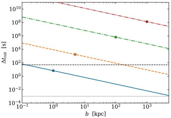
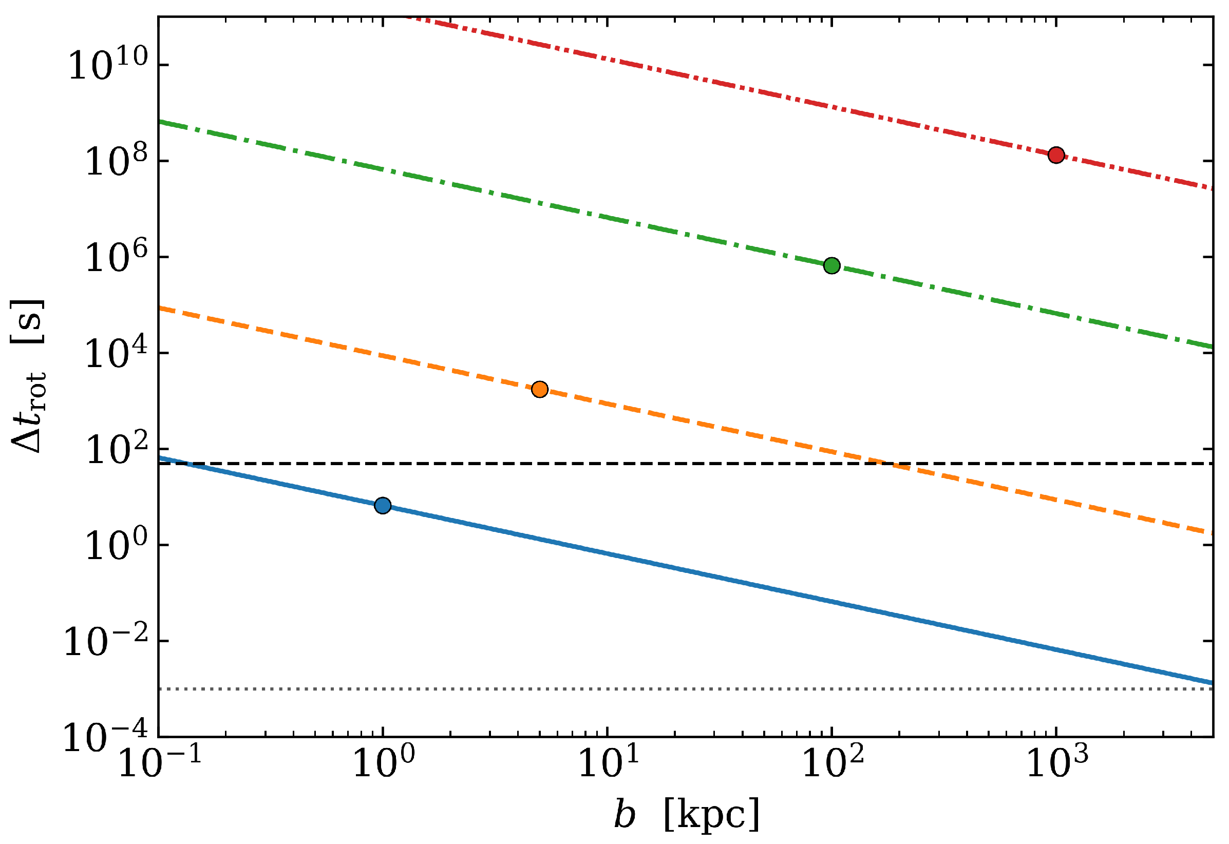
The Milky-Way scale therefore exceeds the minimum by a factor $\sim 30$ in mass, and group- and cluster-scale lenses exceed it by four to seven orders of magnitude (Figure 2). Conversely, dwarf-scale and subhalo clumps fall below the astrometric floor in this channel, which is why the even-parity, time-variable Shapiro channel of Section 5.5—whose sensitivity improves towards small masses—is the complementary probe there. The Newtonian layer is insensitive to this discussion: flattening is measurable for any lens whose images are resolved, and the anomalous $A/b$ falloff (36) is a shape statement, independent of the overall mass scale. The post-Newtonian diagonal layer is closed at ${\beta }^2\sim {10}^{-12}$ for any galactic-scale system and only opens in the ultracompact regime. See Table 2.

Figure 2. Scaling of the parity-odd rotational delay (37) with impact parameter b (horizontal axis, in kpc; vertical axis $\mathsf{\Delta }{t}_{\mathrm{rot}}$ in seconds), for four fiducial clumps spanning subhalo to cluster scales. From bottom to top the curves are: a subhalo, $M={10}^9{M}_{\odot }$, $v=50$ km ${\mathrm{s}}^{-1}$, scale 1 kpc (solid); a Milky-Way-like clump, $6\times {10}^{10}{M}_{\odot }$, 220 km ${\mathrm{s}}^{-1}$, 5 kpc (dashed); a group, ${10}^{13}{M}_{\odot }$, 500 km ${\mathrm{s}}^{-1}$, 100 kpc (dash-dotted); and a cluster, ${10}^{15}{M}_{\odot }$, ${10}^3$ km ${\mathrm{s}}^{-1}$, 1 Mpc (dash-dot-dotted). Filled circles mark b equal to the clump scale. The black dashed horizontal line is the geometric-delay uncertainty implied by 10 μas image astrometry ($\delta t\simeq 50$ s), which is the operative floor; the grey dotted horizontal line is the raw timing precision of lensed fast radio bursts or gravitational-wave chirps (∼1 ms). Milky-Way-scale clumps clear the operative floor by more than an order of magnitude, and are roughly a factor 30 in mass above the threshold (39).

Table 2. Layered observability of the model.

Layer	Observable	Status for a Galactic Clump
$O\left(\beta \right)$	flattening: kinematics, lens ellipticity	routinely measured; fixes $A,\epsilon ,\beta$
$O\left(\beta \right)$	time-variable Shapiro (subhalo transits)	∼10 μs $(M_s/M_{\odot })$ vs. ${10}^2$ ns timing—open for small clumps
$O\left({\beta }^{3/2}\right)$	dragging: precession	${10}^{-3}$μas ${\mathrm{yr}}^{-1}$—closed
$O\left({\beta }^{3/2}\right)$	dragging: lensed-transient $\mathsf{\Delta }{t}_{\mathrm{rot}}$	∼${10}^3$ s vs. ∼50 s astrometric floor—open in principle
$O\left({\beta }^2\right)$	diagonal PN corrections	∼${10}^{-12}$—closed (galactic); $O\left(1\right)$ for mimickers

5.5. Time-Variable Shapiro Delays: The Pulsar-Timing Channel for Small Clumps

For clump masses far below galactic ($M_s\sim {10}^{-2}$–${10}^2{M}_{\odot }$: dark subhalos of Miyamoto–Nagai form), the even-parity Shapiro delay becomes observable through its time variability: a clump transiting near a pulsar line of sight with velocity v modulates the delay by $c\delta t=2{\beta }_s\delta lnw$, with ${\beta }_s=2G{M}_s/c^2$ and w the shifted impact variable of (35), i.e., $\delta t\sim 10\mathsf{\mu }\mathrm{s}(M_s/M_{\odot })$ drifting on the timescale $w/v$. Against the ∼100 ns timing stability of the best millisecond pulsars, decade-long pulsar-timing-array campaigns are sensitive to such transits over a broad subhalo mass range [43]; for the present model the transit template is fully specified by (35), including the $A/b$ anisotropy signature of a disk-like clump. This channel is complementary to the parity-odd channel above: it opens the even sector for small masses, whereas the odd sector probes the angular momentum of large ones.

5.6. Systematics and Honest Limitations

The lensed-transient channel requires a lens with substantial J along a favorable projection, at least two images with well-measured delays, and a mass model constrained well enough that even-parity residuals do not leak into the odd channel; microlensing and plasma delays must be controlled. On the theory side, the model is mean-field—no self-consistent distribution function is constructed, so the closed forms (21)–(23) are statements about the second moments only, and their realizability by a nonnegative distribution function is not established here; the $O\left({\beta }^2\right)$ construction assumes $\beta \ll 1$ for the flattened members, and the linearity claimed for (17) is a property of that expansion, not of the exact system (Section 2.3); the barotropy-Jacobian analysis restricts strict isotropy but not the mixed support; the ansatz (3) assumes meridional isotropy, $P_{\rho }=P_z$, which real discs satisfy only approximately, and relaxing it would require a four-function metric and lies outside the present reduction; the reduction of Section 2.3 presupposes ${(\nabla W)}^2\ne 0$, verified for the present family but not proved in general; and the numerical solution of (17) presented in Section 3.3 is adequate for the second-order metric functions to the accuracy quoted in Table 1, while the thin-disk regime calls for adaptive resolution.

6. Discussion

Relative to the literature known to us, the new elements are: the no-go lemma for $R_{\rho z}$, with its scope explicitly delimited; the identification of the integrability condition of the Weyl-type quadratures with the meridional matter-conservation equations, Equation (12), which is what makes the reduction a genuine solution scheme rather than a formal manipulation; the barotropy Jacobian (19) as a selection criterion for prescribed potentials (rejecting the naive flattened Plummer ansatz and passing Miyamoto–Nagai); the closed forms (21)–(23)—in particular the closed-form stress anisotropy and its unconditional sign—with the decoupling $\mathcal{L}{c}_2=4\kappa P_m$; the closure in which the spatial metric anisotropy $b\ne c$ and the stress anisotropy are derived rather than gauge-fixed (complementary to [8]); the compactness bounds of the spherical member; and the layered observability analysis culminating in the parity-odd delay signature (37) and its scaling (39).

References

- Plummer, H.C. On the problem of distribution in globular star clusters. Mon. Not. R. Astron. Soc. 1911, 71, 460–470. [Google Scholar] [CrossRef] [Scilit]
- Kuzmin, G.G. Model of the steady galaxy allowing of the triaxial distribution of velocities. Astron. Zh. 1956, 33, 27. [Google Scholar]
- Miyamoto, M.; Nagai, R. Three-dimensional models for the distribution of mass in galaxies. Publ. Astron. Soc. Jpn. 1975, 27, 533–543. [Google Scholar] [CrossRef] [Scilit]
- Binney, J.; Tremaine, S. Galactic Dynamics, 2nd ed.; Princeton University Press: Princeton, NJ, USA, 2008. [Google Scholar] [CrossRef] [Scilit]
- Weyl, H. Zur Gravitationstheorie. Ann. Phys. 1917, 54, 117–145. [Google Scholar] [CrossRef] [Scilit]
- Stephani, H.; Kramer, D.; MacCallum, M.A.H.; Hoenselaers, C.; Herlt, E. Exact Solutions of Einstein’s Field Equations, 2nd ed.; Cambridge University Press: Cambridge, UK, 2003. [Google Scholar] [CrossRef] [Scilit]
- Wald, R.M. General Relativity; University of Chicago Press: Chicago, IL, USA, 1984. [Google Scholar]
- Vogt, D.; Letelier, P.S. Relativistic models of galaxies. Mon. Not. R. Astron. Soc. 2005, 363, 268. [Google Scholar] [CrossRef] [Scilit]
- Bičák, J.; Lynden-Bell, D.; Katz, J. Relativistic disks as sources of static vacuum spacetimes. Phys. Rev. D. 1993, 47, 4334–4343. [Google Scholar] [CrossRef] [Scilit] [PubMed]
- Tolman, R.C. Static solutions of Einstein’s field equations for spheres of fluid. Phys. Rev. 1939, 55, 364–373. [Google Scholar] [CrossRef] [Scilit]
- Buchdahl, H.A. General relativistic fluid spheres. Phys. Rev. 1959, 116, 1027–1034. [Google Scholar] [CrossRef] [Scilit]
- Delgaty, M.S.R.; Lake, K. Physical acceptability of isolated, static, spherically symmetric, perfect fluid solutions of Einstein’s equations. Comput. Phys. Commun. 1998, 115, 395–415. [Google Scholar] [CrossRef] [Scilit]
- Rahman, S.; Visser, M. Spacetime geometry of static fluid spheres. Class. Quantum Grav. 2002, 19, 935. [Google Scholar] [CrossRef] [Scilit]
- Lake, K. All static spherically symmetric perfect-fluid solutions of Einstein’s equations. Phys. Rev. D. 2003, 67, 104015. [Google Scholar] [CrossRef] [Scilit]
- Lichtenstein, L. Gleichgewichtsfiguren Rotierender Flüssigkeiten; Springer: Berlin/Heidelberg, Germany, 1933. [Google Scholar]
- Lindblom, L.; Masood-ul-Alam, A.K.M. On the spherical symmetry of static stellar models. Commun. Math. Phys. 1994, 162, 123–145. [Google Scholar] [CrossRef] [Scilit]
- Masood-ul-Alam, A.K.M. Proof that static stellar models are spherical. Gen. Relativ. Gravit. 2007, 39, 55–85. [Google Scholar] [CrossRef] [Scilit]
- Andréasson, H. The Einstein–Vlasov system/kinetic theory. Living Rev. Relativ. 2011, 14, 4. [Google Scholar] [CrossRef] [Scilit] [PubMed]
- Cappellari, M. Structure and kinematics of early-type galaxies from integral field spectroscopy. Annu. Rev. Astron. Astrophys. 2016, 54, 597–665. [Google Scholar] [CrossRef] [Scilit]
- Bowers, R.L.; Liang, E.P.T. Anisotropic spheres in general relativity. Astrophys. J. 1974, 188, 657–665. [Google Scholar] [CrossRef] [Scilit]
- Herrera, L.; Santos, N.O. Local anisotropy in self-gravitating systems. Phys. Rep. 1997, 286, 53–130. [Google Scholar] [CrossRef] [Scilit]
- Chandrasekhar, S. An Introduction to the Study of Stellar Structure; University of Chicago Press: Chicago, IL, USA, 1939. [Google Scholar]
- LeVeque, R.J. Finite Difference Methods for Ordinary and Partial Differential Equations: Steady-State and Time-Dependent Problems; SIAM: Philadelphia, PA, USA, 2007. [Google Scholar] [CrossRef] [Scilit]
- Cardoso, V.; Pani, P. Testing the nature of dark compact objects: A status report. Living Rev. Relativ. 2019, 22, 4. [Google Scholar] [CrossRef] [Scilit]
- Hartle, J.B. Slowly rotating relativistic stars. I. Equations of structure. Astrophys. J. 1967, 150, 1005–1029. [Google Scholar] [CrossRef] [Scilit]
- Hartle, J.B.; Thorne, K.S. Slowly rotating relativistic stars. II. Models for neutron stars and supermassive stars. Astrophys. J. 1968, 153, 807–834. [Google Scholar] [CrossRef] [Scilit] [PubMed]
- Berti, E.; White, F.; Maniopoulou, A.; Bruni, M. Rotating neutron stars: An invariant comparison of approximate and numerical spacetime models. Mon. Not. R. Astron. Soc. 2005, 358, 923–938. [Google Scholar] [CrossRef] [Scilit]
- Tassoul, J.-L. Theory of Rotating Stars; Princeton University Press: Princeton, NJ, USA, 1978. [Google Scholar]
- Chandrasekhar, S. Ellipsoidal Figures of Equilibrium; Yale University Press: New Haven, CT, USA, 1969. [Google Scholar]
- Neugebauer, G.; Meinel, R. General relativistic gravitational field of a rigidly rotating disk of dust: Solution in terms of ultraelliptic functions. Phys. Rev. Lett. 1995, 75, 3046–3047. [Google Scholar] [CrossRef] [Scilit] [PubMed]
- Bland-Hawthorn, J.; Gerhard, O. The Galaxy in context: Structural, kinematic, and integrated properties. Annu. Rev. Astron. Astrophys. 2016, 54, 529–596. [Google Scholar] [CrossRef] [Scilit]
- McMillan, P.J. The mass distribution and gravitational potential of the Milky Way. Mon. Not. R. Astron. Soc. 2017, 465, 76–94, Correction in Mon. Not. R. Astron. Soc. 2017, 466, 174. https://doi.org/10.1093/mnras/stw2759. [Google Scholar] [CrossRef] [Scilit]
- Eilers, A.-C.; Hogg, D.W.; Rix, H.-W.; Ness, M.K. The circular velocity curve of the Milky Way from 5 to 25 kpc. Astrophys. J. 2019, 871, 120. [Google Scholar] [CrossRef] [Scilit]
- GRAVITY Collaboration. A geometric distance measurement to the Galactic center black hole with 0.3% uncertainty. Astron. Astrophys. 2019, 625, L10. [Google Scholar] [CrossRef] [Scilit]
- Bartelmann, M.; Schneider, P. Weak gravitational lensing. Phys. Rep. 2001, 340, 291–472. [Google Scholar] [CrossRef] [Scilit]
- Event Horizon Telescope Collaboration. First M87 Event Horizon Telescope results. I. The Shadow of the Supermassive Black Hole. Astrophys. J. Lett. 2019, 875, L1. [Google Scholar] [CrossRef] [Scilit]
- Everitt, C.W.F.; DeBra, D.B.; Parkinson, B.W.; Turneaure, J.P.; Conklin, J.W.; Heifetz, M.I.; Keiser, G.M.; Silbergleit, A.S.; Holmes, T.; Kolodziejczak, J.; et al. Gravity Probe B: Final results of a space experiment to test general relativity. Phys. Rev. Lett. 2011, 106, 221101. [Google Scholar] [CrossRef] [Scilit] [PubMed]
- Ciufolini, I.; Pavlis, E.C. A confirmation of the general relativistic prediction of the Lense–Thirring effect. Nature 2004, 431, 958–960. [Google Scholar] [CrossRef] [Scilit] [PubMed]
- Will, C.M. The confrontation between general relativity and experiment. Living Rev. Relativ. 2014, 17, 4. [Google Scholar] [CrossRef] [Scilit] [PubMed]
- Abbott, B.P.; Abbott, R.; Abbott, T.D.; Abernathy, M.R.; Acernese, F.; Ackley, K.; Adams, C.; Adams, T.; Addesso, P.; Adhikari, R.X.; et al. Observation of gravitational 692 waves from a binary black hole merger. Phys. Rev. Lett. 2016, 116, 061102. [Google Scholar] [CrossRef] [Scilit] [PubMed]
- Muñoz, J.B.; Kovetz, E.D.; Dai, L.; Kamionkowski, M. Lensing of fast radio bursts as a probe of compact dark matter. Phys. Rev. Lett. 2016, 117, 091301. [Google Scholar] [CrossRef] [Scilit] [PubMed]
- Oguri, M. Strong gravitational lensing of explosive transients. Rep. Prog. Phys. 2019, 82, 126901. [Google Scholar] [CrossRef] [Scilit] [PubMed]
- Dror, J.A.; Ramani, H.; Trickle, T.; Zurek, K.M. Pulsar timing probes of primordial black holes and subhalos. Phys. Rev. D. 2019, 100, 023003. [Google Scholar] [CrossRef] [Scilit]
Disclaimer/Publisher’s Note: The statements, opinions and data contained in all publications are solely those of the individual author(s) and contributor(s) and not of MDPI and/or the editor(s). MDPI and/or the editor(s) disclaim responsibility for any injury to people or property resulting from any ideas, methods, instructions or products referred to in the content. |
© 2026 by the authors. Licensee MDPI, Basel, Switzerland. This article is an open access article distributed under the terms and conditions of the Creative Commons Attribution (CC BY) license.