Induced-Gravity Palatini-like Higgs Inflation in Supergravity Confronts ACT DR6

Abstract

We formulate within Supergravity a model of induced-gravity inflation, excellently consistent with ACT DR6, inspired by the Palatini gravity. The inflaton belongs in the decomposition of a conjugate pair of Higgs superfields which lead to the spontaneous breaking of a $U{\left(1\right)}_{B-L}$ symmetry at a scale close to the range (0.145–8.35) × 10¹⁶ GeV. The inflaton field is canonically normalized thanks to one real and shift-symmetric contribution into the Kähler potential. It also includes two separate holomorphic and antiholomorphic logarithmic terms, the argument of which can be interpreted as the coupling of the inflaton to the Ricci scalar. The attainment of inflation allows for subplanckian inflaton values and energy scales below the cut-off scale of the corresponding effective theory. Embedding the model in a $B-L$ extension of the MSSM we show how the $\mu$ parameter can be generated and non-thermal leptogenesis can be successfully realized. An outcome of our scheme is split SUSY with gravitino mass in the range (40–60) $\mathrm{PeV}$, which is consistent with the results of LHC on the Higgs boson mass.

1. Introduction

The Data Release 6 (DR6) from the Atacama Cosmology Telescope (ACT) [1,2] favors a slightly higher scalar spectral index, $n_{\mathrm{s}}$, than the one indicated from the Planck data [3] prompting renewed interest in inflationary models that can accommodate such a shift [4,5,6,7,8,9,10,11,12,13,14,15,16,17,18,19,20,21,22,23,24,25,26,27,28,29,30,31,32,33,34,35,36,37,38,39,40,41,42,43,44,45,46,47,48,49,50,51,52,53,54,55,56,57]; for a review, see Ref. [58]. Indeed, the combination of the aforementioned data with the measurements from other experiments [3,59,60], also named P-ACT-LB-BK18 data, suggests that $n_{\mathrm{s}}$, its running $a_{\mathrm{s}}$ and the tensor-to-scalar ratio r are to be confined at 95% confidence level (c.l.) in the ranges [2]

$$n_{\mathrm{s}}=0.974\pm 0.0068, a_{\mathrm{s}}=0.0062\pm 0.0104 \mathrm{and} r\le 0.038.$$

(1)

In a recent paper [24] we propose a variant of non-minimal inflation [61,62], characterized as kinetically modified, adopting the Palatini formulation [63,64] of gravity. In particular, we employ a chaotic potential of the form ${\varphi }^n$ for the inflaton field $\varphi$, with $n=2,4$, and a kinetic mixing $f_{\mathrm{K}}=f_{\mathcal{R}}^m$, besides the non-minimal coupling of the inflaton to gravity $f_{\mathcal{R}}=1+c_{\mathcal{R}}{\varphi }^{n/2}$. Our setting causes an elevation in $n_{\mathrm{s}}$, compared to its value in the metric formulation, without an accompanied r increase as we obtained in the last case [65,66,67,68,69]. As a consequence, comfortable compatibility with Equation (1) can be achieved. An outstanding feature of our proposal is the possibility to obtain canonically normalized $\varphi$ for $m=1$, which is not easily feasible in the metric formulation due to an extra term involved in the canonical normalization of $\varphi$. Although Palatini gravity has [70] no Supergravity (SUGRA) embedding, our models in Ref. [24] can be realized within standard (Poincaré) SUGRA thanks to the selected Kähler potential with the $m=1$ case assuring low dimensionality.

In our present investigation we adapt our proposal in Ref. [24] to an elementary Supersymmetric (SUSY) Grand Unified Theory (GUT) performing the following arrangements:

(i)

We promote the inflaton to the radial part of a conjugate pair of superheavy Higgs superfields. This option allows us to focus on the quartic inflationary potential taking $n=4$ in the formulae of Ref. [24]; for other works on GUT-scale Higgs inflation, see, e.g., Refs. [45,67,68,69,71,72,73,74,75,76,77,78,79,80,81].

(ii)

We restrict ourselves to a Kähler potential with just quadratic contributions. Similarly to the case with gauge-singlet inflation [24], this second assumption leads to canonical kinetic terms for the inflaton. As a consequence, we reveal a model recently analyzed in Ref. [82] with focus on its consistency with unitarity [83,84,85,86,87,88,89].

(iii)

We incorporate the idea of Induced Gravity (IG) [90] according to which the (reduced) Planck mass $m_{\mathrm{P}}$ is generated via the vacuum expectation value (v.e.v) that a scalar field acquires at the end of a phase transition in the early universe. In our scheme, the scalar field is identified with the Higgsflaton—cf. Refs. [71,80,81,91,92,93,94,95,96,97,98,99,100].

(iv)

We connect the strength of the non-minimal coupling to gravity with the scale of the unification of the gauge coupling constants of the Minimal SUSY Standard Model (MSSM)—cf. Refs. [80,81].

The hypotheses above give rise to an economical, predictive and well-motivated set-up, which can be characterized, following the terminology of Ref. [24], as (kinetically modified with $m=1$) induced-gravity Palatini-like Higgs inflation (IPI). This construction actually “ACT-ivates” our older models in Refs. [80,81], which may become consistent with Equation (1) only at the cost of some tuning regarding the coefficients of the logarithm in the Kähler potentials. This tuning can be totally avoided in our present model, although we discuss, just for completeness, the behavior of our results with variation of the relevant coefficient (N).

Apart from the compatibility with Equation (1), IPI offers also the opportunity to explore consequences beyond the inflationary phenomenology. Namely, by embedding it into a $B-L$ extension of MSSM, we can accommodate a resolution of the $\mu$ problem, following the mechanism in Refs. [80,81,101], and acceptable baryogenesis via non-thermal leptogenesis (nTL) [102,103,104] consistently with gravitino ($\tilde{G}$) cosmology [105,106,107]. Contrary to previous implementations of the same post-inflationary scheme—cf. Refs. [45,79,80,81]— the outcome here includes split SUSY [108,109,110] with very short-lived $\tilde{G}$.

The remaining text is structured as follows. In Section 2 we present the cornerstones of our proposal and, in Section 3, we analyze the inflationary scenario. We then, in Section 4, examine a possible post-inflationary completion of our setting. Our conclusions are summarized in Section 5. In Appendix A we address a subtlety related to a very short stage of oscillating inflation (OI) [111,112,113,114] encountered after the end of IPI. Throughout the text, the subscript of type, $z$ denotes derivation with respect to (w.r.t) the field z and charge conjugation is denoted by a star. Unless otherwise stated, we use units where $m_{\mathrm{P}}=2.43·{10}^{18} \mathrm{GeV}$ is taken to be unity.

2. Higgs Inflation and Induced Gravity

In Section 2.1 we specify the relevant super- and Kähler potential of our proposal, whereas in Section 2.2 we explain the imposition of the IG condition.

2.1. Set-Up

Our starting point is the superpotential known from the models of F-term hybrid inflation [37,38,39,40,41]

$$W_{\mathrm{IPI}}=\lambda S\left(\overline{\mathsf{\Phi }}\mathsf{\Phi }-M^2/4\right)$$

(2)

which is uniquely determined, at renormalizable level, by a gauge symmetry $\mathbb{G}$ and a convenient continuous R symmetry. Here, $\lambda$ and M are two constants which can both be taken positive by field redefinitions; S is a left-handed superfield, singlet under $\mathbb{G}$; $\overline{\mathsf{\Phi }}$ and $\mathsf{\Phi }$ is a pair of left-handed superfields belonging to non-trivial conjugate representations of $\mathbb{G}$, and reducing its rank by their v.e.vs. Just for definiteness we restrict ourselves to ${\mathbb{G}}_{B-L}={\mathbb{G}}_{\mathrm{SM}}\times U{\left(1\right)}_{B-L}$ which consists the simplest GUT beyond the MSSM; here, ${\mathbb{G}}_{\mathrm{SM}}$ is the gauge group of MSSM and B and L denote the baryon and lepton numbers. With the specific choice of $\mathbb{G}$, the $U{\left(1\right)}_{B-L}$ and R charges of the various superfields are

$$(B-L)(S,\overline{\mathsf{\Phi }},\mathsf{\Phi })=(0,-2,2) \mathrm{and} R(S,\overline{\mathsf{\Phi }},\mathsf{\Phi })=(2,0,0).$$

(3)

At the SUSY limit, we expect that W leads to a $B-L$ phase transition as we show in Section 2.2.2 below.

The realization of IPI with the inflaton included in the $\overline{\mathsf{\Phi }}-\mathsf{\Phi }$ system and S stabilized at the origin requires a careful choice of K—as, e.g., in Refs. [69,77,78,80]. The herein proposed K includes two contributions without mixing between the $\overline{\mathsf{\Phi }}-\mathsf{\Phi }$ and S sectors. Namely, it is written as

$$K=K_{\mathrm{I}}+K_{\mathrm{st}}.$$

(4)

The second term in K successfully stabilizes S at the origin without invoking higher order terms—cf. Ref. [115]. In particular, $K_{\mathrm{st}}$ takes the form

$$K_{\mathrm{st}}=N_{\mathrm{st}}ln\left(1+{|S|}^2/N_{\mathrm{st}}\right) \mathrm{with} 0<N_{\mathrm{st}}<6$$

(5)

which parametrizes [116] the compact manifold $SU\left(2\right)/U\left(1\right)$ with curvature $2/N$. On the other hand, $K_{\mathrm{I}}$ depends on the $\overline{\mathsf{\Phi }}-\mathsf{\Phi }$ sector and includes the functions

$$F_{\mathcal{R}}\left(\mathsf{\Phi }\right)=4c_{\mathcal{R}}\overline{\mathsf{\Phi }}\mathsf{\Phi } \mathrm{and} F_{\mathrm{sh}}={|\mathsf{\Phi }-{\overline{\mathsf{\Phi }}}^{*}|}^2,$$

(6)

from which $F_{\mathcal{R}}$ is holomorphic and can be employed as the non-minimal coupling to gravity, whereas $F_{\mathrm{sh}}$ is real, assisting us to incorporate the canonical kinetic mixing. These functions extend the corresponding ones in Ref. [24] to the case of a conjugate pair of gauge non-singlet superfields $\overline{\mathsf{\Phi }}-\mathsf{\Phi }$. In sharp contrast to those functions, however, unity is not included in $F_{\mathcal{R}}$. As explained in Section 2.2, the identification of $F_{\mathcal{R}}$ with unity at the vacuum of the theory essentially encapsulates the IG hypothesis—cf. Refs. [80,81,95,98,100,101]. With the ingredients above, we construct $K_{\mathrm{I}}$ in Equation (4) which is

$$K_{\mathrm{I}}=-{\displaystyle \frac{N}{2}}ln{F}_{\mathcal{R}}-{\displaystyle \frac{N}{2}}ln{F}_{\mathcal{R}}^{*}+F_{\mathrm{sh}}$$

(7)

and features the structure of $K_{\mathrm{I}}$ in Ref. [24]—at renormalizable level, i.e., $m=1$—with the introduction of variable coefficients of the logarithms. It is worth noticing that contrary to the embedding of IG Higgs inflation in metric SUGRA—cf. Refs. [80,81]—$F_{\mathcal{R}}$ and $F_{\mathcal{R}}^{*}$ enter two different terms in Equation (7) and so they give zero contribution into the Kähler metric, which takes the form

$$M_{\overline{\mathsf{\Phi }}\mathsf{\Phi }}=\left(K_{\mathrm{I}\alpha \overline{\beta }}\right)=\mathsf{diag}\left(1,1\right),$$

(8)

where we use the standard notation $K_{\mathrm{I}\alpha \overline{\beta }}=K_{\mathrm{I},z^{\alpha }{z}^{*\overline{\beta }}}$ with $z^{\alpha }=\mathsf{\Phi },\overline{\mathsf{\Phi }}$. Alternative forms of K in Equation (4) as those discussed in Ref. [80] can be also constructed using variants of $K_{\mathrm{st}}$ in Equation (5) and changing its placement in the logarithms of $K_{\mathrm{I}}$. We adopt here the simplest option which enjoys an exact symmetry regarding $K_{\mathrm{st}}$.

2.2. Implementation of IG Condition

The scale M and the function $F_{\mathcal{R}}$ involved in Equations (2) and (7) assist us in implementing the idea of IG. To explain how it works, we introduce our notation in the Einstein and Jordan frames in Section 2.2.1 and then, in Section 2.2.2, we derive the SUSY vacuum which plays a key role in imposing the IG condition.

2.2.1. From Einstein to Jordan Frame

The part of the Einstein frame (EF) action within SUGRA related to the complex scalars $z^{\alpha }=\mathsf{\Phi },\overline{\mathsf{\Phi }},S$—denoted by the same superfield symbol—has the form [115]

$$\mathsf{S}=\int d^{4}x\sqrt{-\widehat{\mathfrak{g}}}\left(-{\displaystyle \frac{1}{2}}\widehat{\mathcal{R}}+K_{\alpha \overline{\beta }}{\widehat{g}}^{\mu \nu }{D}_{\mu }{z}^{\alpha }{D}_{\nu }{z}^{*\overline{\beta }}-\widehat{V}\right),$$

(9a)

where $\widehat{\mathfrak{g}}$ is the determinant of the EF metric ${\widehat{g}}_{\mu \nu }$, $\widehat{\mathcal{R}}$ is the EF Ricci scalar curvature, $D_{\mu }$ is the gauge covariant derivative, and $K^{\alpha \overline{\beta }}$ is the inverse of the Kähler metric defined as $K^{\alpha \overline{\beta }}{K}_{\overline{\beta }\gamma }={\delta }_{\gamma }^{\alpha }$. Also, $\widehat{V}$ is the EF SUGRA potential, which includes F- and D- term contributions, which can be found in terms of W and K in Equations (2) and (4) via the formula

$$\widehat{V}=e^K\left(K^{\alpha \overline{\beta }}\left(D_{\alpha }{W}_{\mathrm{IPI}}\right)D_{\overline{\beta }}^{*}{W}_{\mathrm{IPI}}^{*}-3|W_{\mathrm{IPI}}{|}^2\right)+{\displaystyle \frac{g^2}{2}}{\mathrm{D}}_{BL}^2,$$

(9b)

where g is the gauge coupling constant—assumed unified with the others of ${\mathbb{G}}_{\mathrm{SM}}$–and we define the Kähler covariant derivative and the D terms due to ${\mathbb{G}}_{B-L}$ as

$$D_{\alpha }{W}_{\mathrm{IPI}}=W_{\mathrm{IPI},z^{\alpha }}+K_{,z^{\alpha }}{W}_{\mathrm{IPI}} \mathrm{and} {\mathrm{D}}_{BL}=\mathsf{\Phi }{K}_{\mathsf{\Phi }}-\overline{\mathsf{\Phi }}{K}_{\overline{\mathsf{\Phi }}}=\left({|\mathsf{\Phi }|}^2-{|\overline{\mathsf{\Phi }}|}^2\right).$$

(10)

Therefore, a field configuration with vanishing ${\mathrm{D}}_{BL}$ is

$${⟨\mathsf{\Phi }⟩}_{\mathrm{I}}={⟨\overline{\mathsf{\Phi }}⟩}_{\mathrm{I}}=\varphi /2 \mathrm{and} {⟨S⟩}_{\mathrm{I}}=0,$$

(11)

where take into account additionally the stabilization of S and we introduce the symbol ${⟨\dots ⟩}_{\mathrm{I}}$ to denote values during IPI. Henceforth, we confine ourselves to this path—assuming furthermore that $\mathsf{arg}\left(\mathsf{\Phi }\right)=\mathsf{arg}\left(\overline{\mathsf{\Phi }}\right)$—which is a honest inflationary trajectory, as we show in Section 3.1, supporting IPI driven exclusively by ${\widehat{V}}_{\mathrm{F}}$.

The action in Equation (9a) can be brought into the Jordan frame (JF) by performing a conformal transformation [69,115]. As clarified in Ref. [70], SUGRA admits only metric formulation and, therefore, if we define the JF metric, $g_{\mu \nu }$, through the relation

$${\widehat{g}}_{\mu \nu }=-(\mathsf{\Omega }/N)g_{\mu \nu },$$

(12a)

where $\mathsf{\Omega }$ is the frame function, we are obliged to adopt the well-known relations between hatted (EF) and unhatted (JF) quantities mentioned in Refs. [69,80]. As a consequence, we end up with the following action in the JF

$$\mathsf{S}=\int d^{4}x\sqrt{-\mathfrak{g}}\left({\displaystyle \frac{\mathsf{\Omega }{m}_{\mathrm{P}}^2}{2N}}\mathcal{R}+{\displaystyle \frac{3m_{\mathrm{P}}^2}{4N\mathsf{\Omega }}}{D}_{\mu }\mathsf{\Omega }{D}^{\mu }\mathsf{\Omega }-{\displaystyle \frac{1}{N}}\mathsf{\Omega }{K}_{\alpha \overline{\beta }}{D}_{\mu }{z}^{\alpha }{D}^{\mu }{z}^{*\overline{\beta }}-V\right) \mathrm{with} V={\displaystyle \frac{{\mathsf{\Omega }}^2}{N^2}}\widehat{V}.$$

(12b)

If, in addition, we connect $\mathsf{\Omega }$ to K in Equation (4) through the following relation

$$-\mathsf{\Omega }/N=e^{-K/N{m}_{\mathrm{P}}^2}=F_{\mathcal{R}}^{1/2}{F}_{\mathcal{R}}^{*1/2}{e}^{-F_{\mathrm{sh}}/N}{(1+|S|}^2/N_{\mathrm{st}}{m}_{\mathrm{P}}^2{)}^{-N_{\mathrm{st}}/N}$$

(13a)

we arrive at the following action

$$\mathsf{S}=\int d^{4}x\sqrt{-\mathfrak{g}}\left({\displaystyle \frac{\mathsf{\Omega }}{2N}}{m}_{\mathrm{P}}^2\mathcal{R}+m_{\mathrm{P}}^2\left({\mathsf{\Omega }}_{\alpha \overline{\beta }}+{\displaystyle \frac{3-N}{N}}{\displaystyle \frac{{\mathsf{\Omega }}_{\alpha }{\mathsf{\Omega }}_{\overline{\beta }}}{\mathsf{\Omega }}}\right)D_{\mu }{z}^{\alpha }{D}^{\mu }{z}^{*\overline{\beta }}-{\displaystyle \frac{27}{N^3}}\mathsf{\Omega }{\mathcal{A}}_{\mu }{\mathcal{A}}^{\mu }-V\right),$$

(13b)

where we take into account the definition [115] of the purely bosonic part of the on-shell value of the auxiliary field

$${\mathcal{A}}_{\mu }=i\left(K_{\alpha }{D}_{\mu }{z}^{\alpha }-K_{\overline{\alpha }}{D}_{\mu }{z}^{*\overline{\alpha }}\right)/6=-iN{m}_{\mathrm{P}}^2\left({\mathsf{\Omega }}_{\alpha }{D}_{\mu }{z}^{\alpha }-{\mathsf{\Omega }}_{\overline{\alpha }}{D}_{\mu }{z}^{*\overline{\alpha }}\right)/6\mathsf{\Omega }.$$

(13c)

Here we use the shorthand notation ${\mathsf{\Omega }}_{\alpha }={\mathsf{\Omega }}_{,{\mathsf{\Phi }}^{\alpha }}$ and ${\mathsf{\Omega }}_{\overline{\alpha }}={\mathsf{\Omega }}_{,{\mathsf{\Phi }}^{*\overline{\alpha }}}$. The first term in the right-hand side of Equation (13b) reveals that $-\mathsf{\Omega }/N$ plays the role of a non-minimal coupling to gravity. The emergence of the conventional Einstein gravity at the vacuum dictates

$$-⟨\mathsf{\Omega }/N⟩=1,$$

(14)

where we restore the presence of $m_{\mathrm{P}}$ in the last expressions above for convenience.

2.2.2. IG Conjecture

The IG hypothesis requires the generation of $m_{\mathrm{P}}$ at the vacuum of the theory, which can be determined expanding $\widehat{V}$ in Equation (9a) in powers of $1/m_{\mathrm{P}}$. Namely, we obtain the following low-energy effective potential which plays the role of the SUSY one

$$V_{\mathrm{SUSY}}=e^{\tilde{K}}{\tilde{K}}^{\alpha \overline{\beta }}{W}_{\mathrm{IPI}\alpha }{W}_{\mathrm{IPI}\overline{\beta }}^{*},$$

(15a)

where $\tilde{K}$ is the limit of K in Equation (4) for $m_{\mathrm{P}}\to \infty$. Namely, we get

$$\tilde{K}=-Nln{\left(F_{\mathcal{R}}{F}_{\mathcal{R}}^{*}\right)}^{1/2}+|\mathsf{\Phi }-{\overline{\mathsf{\Phi }}}^{*}{|}^2+{|S|}^2,$$

(15b)

from which we can then compute the Kähler metric ${\tilde{K}}_{\alpha \overline{\beta }}=\mathsf{diag}(1,1,1)$. Upon substitution into Equation (15a) we obtain

$$V_{\mathrm{SUSY}}\simeq {\left(F_{\mathcal{R}}{F}_{\mathcal{R}}^{*}\right)}^{-N/2}\left(({\lambda }^2{\left|\overline{\mathsf{\Phi }}\mathsf{\Phi }-M^2/4\right|}^2+{\lambda }^2|S{|}^2\left({|\mathsf{\Phi }|}^2+{|\overline{\mathsf{\Phi }}|}^2\right)\right).$$

(16)

We can easily infer that the SUSY vacuum lies along the direction

$$⟨S⟩=0 \mathrm{and} |⟨\mathsf{\Phi }⟩|=|⟨\overline{\mathsf{\Phi }}⟩|=M/2\Rightarrow ⟨\varphi ⟩=M,$$

(17)

which is included in the inflationary path of Equation (43). As we see below—in Section 4.2—$⟨S⟩$ may slightly deviate from its value above after inclusion of soft SUSY-breaking effects. From Equation (17) it is clear that $⟨\mathsf{\Phi }⟩$ and $⟨\overline{\mathsf{\Phi }}⟩$ spontaneously break $U{\left(1\right)}_{B-L}$ down to ${\mathbb{Z}}_2^{B-L}$. Note that $U{\left(1\right)}_{B-L}$ is already broken during IPI and so no cosmic strings are formed—see Section 3.2.

The scale of $U{\left(1\right)}_{B-L}$ breaking can be related to the magnitude of $c_{\mathcal{R}}$ via the IG conjecture in Equation (14). Indeed, upon substitution of Equation (17) into Equation (13a), Equation (14) implies

$$c_{\mathcal{R}}{⟨\varphi ⟩}^2/m_{\mathrm{P}}^2=1 \stackrel{\left(17\right)}{⟹} M=m_{\mathrm{P}}/\sqrt{c_{\mathcal{R}}}.$$

(18)

As we see below, both $c_{\mathcal{R}}$ and M can be independently restricted by the inflationary and the gauge unification requirements correspondingly enhancing, thereby, the predictability of the model.

3. Inflation Analysis

We below—in Section 3.1—derive the inflationary potential of our model and then present its predictions in Section 3.2.

3.1. Inflationary Potential

If we parameterize $\mathsf{\Phi },\overline{\mathsf{\Phi }}$ and S as follows

$$\mathsf{\Phi }={\displaystyle \frac{1}{\sqrt{2}}}\varphi e^{i\theta }cos{\theta }_{\mathsf{\Phi }}, \overline{\mathsf{\Phi }}={\displaystyle \frac{1}{\sqrt{2}}}\varphi e^{i\overline{\theta }}sin{\theta }_{\mathsf{\Phi }} \mathrm{where} 0\le {\theta }_{\mathsf{\Phi }}\le {\displaystyle \frac{\pi }{2}} \mathrm{and} S={\displaystyle \frac{1}{\sqrt{2}}}\left(s+i\overline{s}\right),$$

(19)

the D-flat direction in Equation (11) can be now expressed as

$${⟨s⟩}_{\mathrm{I}}={⟨\overline{s}⟩}_{\mathrm{I}}={⟨\theta ⟩}_{\mathrm{I}}={⟨\overline{\theta }⟩}_{\mathrm{I}}=0 \mathrm{and} {⟨{\theta }_{\mathsf{\Phi }}⟩}_{\mathrm{I}}=\pi /4.$$

(20)

Along this, the only surviving term of $\widehat{V}$ in Equation (9b) can be written as

$${\widehat{V}}_{\mathrm{IPI}}=e^K{K}^{S{S}^{*}}{|W_{\mathrm{IPI},S}|}^2={\displaystyle \frac{{\lambda }^2{({\varphi }^2-M^2)}^2}{16f_{\mathcal{R}}^N}}={\displaystyle \frac{{\lambda }^2{f}_{\mathrm{W}}^2}{16c_{\mathcal{R}}^{2+N}{\varphi }^{2N}}},$$

(21a)

where we define the following quantities

$$f_{\mathcal{R}}=-⟨\mathsf{\Omega }/N{⟩}_{\mathrm{I}}=c_{\mathcal{R}}{\varphi }^2, f_{\mathrm{W}}=c_{\mathcal{R}}{\varphi }^2-1 \mathrm{and} N=2(1+\delta N).$$

(21b)

Note that we make use of Equation (18) for the derivation of the last expression in Equation (21a). This one clearly reveals the fact that the minimum of ${\widehat{V}}_{\mathrm{IPI}}$ is not placed at zero—as in the original Starobinsky model [101]—but at $\varphi =⟨\varphi ⟩$ given in Equation (17). This is evidently due to the adoption of the IG conjecture [95,98,100] which allows us to obtain a Starobinsky-like potential. Indeed, for $N=2$ ${\widehat{V}}_{\mathrm{IPI}}$ develops an inflationary plateau, with potential energy density ${\widehat{V}}_{\mathrm{IPI}0}$ and corresponding Hubble parameter ${\widehat{H}}_{\mathrm{IPI}}$ given respectively by

$${\widehat{V}}_{\mathrm{IPI}0}\simeq {\displaystyle \frac{{\lambda }^2}{16c_{\mathcal{R}}^2}} \mathrm{and} {\widehat{H}}_{\mathrm{IPI}}\simeq {\displaystyle \frac{{\widehat{V}}_{\mathrm{IPI}0}^{1/2}}{\sqrt{3}}}={\displaystyle \frac{\lambda }{4c_{\mathcal{R}}\sqrt{3}}},$$

(22)

in accordance with the well-known Starobinsky-like inflationary models [95,98,101]. However, $\delta N$ allows for slight deviations from the absolute flatness as in the cases analyzed in Refs. [80,81,93]. In contrast to those metric realizations of Starobinsky inflation, in our present case, the inflaton (and S) is canonically normalized since $K_{\alpha \overline{\beta }}$ along the path in Equation (20) is trivial, i.e.,

$${⟨K_{\alpha \overline{\beta }}⟩}_{\mathrm{I}}=\mathsf{diag}\left(1,1,1\right).$$

(23)

This is a consequence of the shift-symmetric real part in Equation (7) which can be interpreted as a kinetic modification of the Palatini inflation motivated in Ref. [24] and analyzed recently in Ref. [82] with focus on the issue of unitarity. Adopting the notation of Ref. [24] we here use $m=1$ and not $m=0$ which corresponds to the original (i.e., kinetically unmodified) model of Palatini inflation [63,64]. Needless to say, the derivation of the Starobinsky potential is here based exclusively on the structure of $\widehat{V}$ in Equation (9b) and not on a specific relation between the initial and the canonically normalized inflaton as in case of E- [117,118] or T-model [119,120,121].

We can verify that the inflationary direction in Equation (20) is stable w.r.t the fluctuations of the fields ${\chi }^{\alpha }={\theta }_{+},{\theta }_{\mathsf{\Phi }}$ and S where ${\theta }_{\pm }=\left(\overline{\theta }\pm \theta \right)/\sqrt{2}$. To this end, we construct the mass-squared spectrum of those scalars and arrange the found expressions in Table 1. These expressions assist us to appreciate the role of $N_{\mathrm{st}}>0$ in retaining positive $m_S^2$. Moreover, $m_{{\chi }^{\alpha }}^2\gg {\widehat{H}}_{\mathrm{IPI}}^2={\widehat{V}}_{\mathrm{IPI}0}/3$ for ${\varphi }_{\mathrm{f}}\le \varphi \le {\varphi }_{★}$—the field values ${\varphi }_{★}$ and ${\varphi }_{\mathrm{f}}$ are specified in Section 3.2.1 below. In Table 1 we display also the masses, $M_{BL}$, of the gauge boson $A_{BL}$ and the masses of the corresponding fermions with the eigenstate ${\widehat{\psi }}_{\pm }$ defined as ${\psi }_{\pm }=({\psi }_{\mathsf{\Phi }+}\pm {\psi }_S)/\sqrt{2}$. Since ${\mathbb{G}}_{B-L}$ is broken during IPI, no cosmic strings are formed after its termination.

Table 1. The mass-squared spectrum of our model along the configuration in Equation (20).

Fields	Eingestates	Masses Squared
4 Real	${\theta }_{+}$	$m_{\theta +}^2$	$3(1+4c_{\mathcal{R}}/f_{\mathrm{W}}^2){\widehat{H}}_{\mathrm{IPI}}^2$
Scalars	${\theta }_{\mathsf{\Phi }}$	$m_{{\theta }_{\mathsf{\Phi }}}^2$	$M_{BL}^2+6(1-4c_{\mathcal{R}}/f_{\mathrm{W}}+4(1+\delta N)/{\varphi }^2){\widehat{H}}_{\mathrm{IPI}}^2$
	$s,\overline{s}$	$m_s^2$	$6(1/N_{\mathrm{st}}+4/{\varphi }^2{f}_{\mathrm{W}}^2){\widehat{H}}_{\mathrm{IPI}}^2$
1 Gauge Boson	$A_{BL}$	$M_{BL}^2$	$g^2{\varphi }^2$
7 Weyl	${\psi }_{\pm }$	$m_{\psi \pm }^2$	$24{(1-\delta N{f}_{\mathrm{W}})}^2{\widehat{H}}_{\mathrm{IPI}}^2/f_{\mathrm{W}}^2{\varphi }^2$
Spinors	${\mathsf{\lambda }}_{BL},{\psi }_{\mathsf{\Phi }-}$	$M_{BL}^2$	$g^2{\varphi }^2$

The derived mass spectrum can be employed in order to find the one-loop radiative corrections $\mathsf{\Delta }{V}_{\mathrm{I}}$ to ${\widehat{V}}_{\mathrm{IPI}}$. Considering SUGRA as an effective theory with cutoff scale equal to $m_{\mathrm{P}}$, the well-known Coleman-Weinberg formula can be employed self-consistently taking into account only the masses which lie well below the UV cut-off scale ${\mathsf{\Lambda }}_{\mathrm{UV}}$—see Section 3.2.2 below – i.e., all the masses arranged in Table 1 besides $M_{BL}$ and $m_{{\theta }_{\mathsf{\Phi }}}$—cf. Refs. [69,77]. The resulting $\mathsf{\Delta }{V}_{\mathrm{I}}$ takes the form

$$\mathsf{\Delta }{V}_{\mathrm{I}}={\displaystyle \frac{1}{64{\pi }^2}}\sum _{\alpha }{\mathrm{N}}_{\alpha }{m}_{\alpha }^{4}ln{\displaystyle \frac{m_{\alpha }^2}{{\mathsf{\Lambda }}_{\mathrm{CW}}^2}} \mathrm{where} \left\{\begin{array}{cc}\alpha \hfill & =\{{\theta }_{+},s,{\psi }_{\mathsf{\Phi }\pm }\}\hfill \\ {\mathrm{N}}_{\alpha }\hfill & =\{1,2,-4\}\hfill \end{array}\right.$$

(24)

and lets intact our inflationary outputs, provided that the renormalization-group mass scale ${\mathsf{\Lambda }}_{\mathrm{CW}}$, is determined by requiring $\mathsf{\Delta }{V}_{\mathrm{I}}\left({\varphi }_{★}\right)=0$ or $\mathsf{\Delta }{V}_{\mathrm{I}}\left({\varphi }_{\mathrm{f}}\right)=0$. Specific values of ${\mathsf{\Lambda }}_{\mathrm{CW}}$ are given in Section 3.3.2 below.

3.2. Inflationary Observables—Constraints

The constraints imposed on our inflationary setting may be grouped in two categories (observational and theoretical) which are described respectively in Section 3.2.1 and Section 3.2.2 below.

3.2.1. Observational Constraints

These constraints reconcile our model with the present data [2]. Namely, they are related to:

(a)

Normalization of the Power Spectrum and Number of e-foldings.

The amplitude $A_{\mathrm{s}}$ of the power spectrum of the curvature perturbations generated by $\varphi$ and the number of e-foldings ${\widehat{N}}_{★}$ that the scale $k_{★}=0.05/\mathrm{Mpc}$ experiences during IPI can be computed using the standard formulae [122]

$$A_{\mathrm{s}}^{1/2}={\displaystyle \frac{1}{2\sqrt{3}\pi }}{\displaystyle \frac{{\widehat{V}}_{\mathrm{IPI}}^{3/2}\left({\varphi }_{★}\right)}{\left|{\widehat{V}}_{\mathrm{IPI},\varphi }\left({\varphi }_{★}\right)\right|}} \mathrm{and} {\widehat{N}}_{★}={\int }_{{\varphi }_{\mathrm{f}}}^{{\varphi }_{★}}d\varphi {\displaystyle \frac{{\widehat{V}}_{\mathrm{IPI}}}{{\widehat{V}}_{\mathrm{IPI},\varphi }}},$$

(25)

where ${\varphi }_{★}$ is the value of $\varphi$ when $k_{★}$ crosses outside the inflationary horizon, and ${\varphi }_{\mathrm{f}}$ is the value of $\varphi$ at the end of IPI, which can be found, in the slow-roll approximation, from the condition

$$\mathsf{max}\left\{\widehat{ϵ}\left(\varphi \right),\left|\widehat{\eta }\left(\varphi \right)\right|\right\}\simeq 1, \mathrm{where} \widehat{ϵ}={\displaystyle \frac{1}{2}}{\left({\displaystyle \frac{{\widehat{V}}_{\mathrm{IPI},\varphi }}{{\widehat{V}}_{\mathrm{IPI}}}}\right)}^2 \mathrm{and} \widehat{\eta }={\displaystyle \frac{{\widehat{V}}_{\mathrm{IPI},\varphi \varphi }}{{\widehat{V}}_{\mathrm{IPI}}}}·$$

(26)

The observables above are to be confronted with the [2]

$$\begin{array}{c}\sqrt{A_{\mathrm{s}}}\simeq 4.618·{10}^{-5} \mathrm{and} {\widehat{N}}_{★}\simeq 61.5+ln{\displaystyle \frac{{\widehat{V}}_{\mathrm{IPI}}{\left({\varphi }_{★}\right)}^{1/2}}{{\widehat{V}}_{\mathrm{IPI}}{\left({\varphi }_{\mathrm{of}}\right)}^{1/4}}}-{\displaystyle \frac{1}{3(1+w_{\mathrm{oi}})}}ln{\displaystyle \frac{{\widehat{V}}_{\mathrm{IPI}}\left({\varphi }_{\mathrm{f}}\right)}{{\widehat{V}}_{\mathrm{IPI}}\left({\varphi }_{\mathrm{of}}\right)}}\hfill \\ +{\displaystyle \frac{1-3w_{\mathrm{rh}}}{6(1+w_{\mathrm{rh}})}}\left(ln{\left({\rho }_{\mathrm{rh}}/{\widehat{V}}_{\mathrm{IPI}}\left({\varphi }_{\mathrm{of}}\right)\right)}^{1/2}-ln{f}_{\mathcal{R}}\left({\varphi }_{\mathrm{f}}\right)\right)+{\displaystyle \frac{1}{2}}{f}_{\mathcal{R}}\left({\varphi }_{★}\right).\hfill \end{array}$$

(27)

Here, we take into account—see Appendix A—that IPI is followed in turn by a very short period of OI and a phase of damped oscillations with mean equation-of-state parameters $w_{\mathrm{oi}}\simeq -0.71$ and $w_{\mathrm{rh}}\simeq -0.02$ respectively. Note that $w_{\mathrm{rh}}$ is approximately equal to the value we obtain for a quadratic potential [123,124] and not quartic as naively expected from the form of numerator of ${\widehat{V}}_{\mathrm{IPI}}$ in Equation (21a). Also $T_{\mathrm{rh}}$ is the temperature after IPI with correspoding energy density

$${\rho }_{\mathrm{rh}}={\pi }^2{g}_{\mathrm{rh}\ast }{T}_{\mathrm{rh}}^4/30 \mathrm{where} g_{\mathrm{rh}\ast }=228.75$$

(28)

is the energy-density effective number of degrees of freedom for the MSSM spectrum at the reheat temperature $T_{\mathrm{rh}}$. After reheating we obtain the well-known radiation and matter domination.

(b)

Remaining Observables.

The compatibility with the data in Equation (1) can be checked if we compute the corresponding inflationary observables through the relations:

$$\left(\mathsf{a}\right) n_{\mathrm{s}}=1-6{\widehat{ϵ}}_{★}+2{\widehat{\eta }}_{★}, \left(\mathsf{b}\right) a_{\mathrm{s}}=2\left(4{\widehat{\eta }}_{★}^2-{(n_{\mathrm{s}}-1)}^2\right)/3-2{\widehat{\xi }}_{★} \mathrm{and} \left(\mathsf{c}\right) r=16{\widehat{ϵ}}_{★},$$

(29)

where $\widehat{\xi }={\widehat{V}}_{\mathrm{IPI},\varphi }{\widehat{V}}_{\mathrm{IPI},\varphi \varphi \varphi }/{\widehat{V}}_{\mathrm{IPI}}^2$ and the variables with subscript $★$ are evaluated at $\varphi ={\varphi }_{★}$.

3.2.2. Theoretical Considerations

We may qualify better our models by taking into account three additional restrictions of theoretical origin. In particular, we consider the following issues:

(a)

Connection With the Gauge Coupling Unification

The $U{\left(1\right)}_{B-L}$ gauge symmetry does not generate any extra contribution to the renormalization group running of the gauge coupling constants of ${\mathbb{G}}_{\mathrm{SM}}$ and so the scale M and the relevant gauge coupling constant, g can be different than the values dictated by the MSSM unification of the gauge coupling constants which gives $g\simeq 0.7$ with $M_{\mathbb{G}}\simeq 20 \mathrm{YeV}$. Note that this result is valid also in case of split SUSY [109] which fits well with our scheme—see Section 4.2. In our approach we mostly keep the g value above and let $M_{\mathbb{G}}$ varying. The connection with IG condition can be done if we identify $M_{\mathbb{G}}$ with the mass of the gauge boson, $M_{BL}$ in Table 1, computed at the vacuum of Equation (17), $⟨M_{BL}⟩$. Such an approach allows to find $c_{\mathcal{R}}$ in terms of $M_{\mathrm{GUT}}$ as follows

$$⟨M_{BL}⟩=g⟨\varphi ⟩=M_{\mathbb{G}}\stackrel{\left(18\right)}{⟹}{c}_{\mathcal{R}}=g^2{m}_{\mathrm{P}}^2/M_{\mathbb{G}}^2.$$

(30)

It is beneficial that our scheme independently constrains the allowed margin of $M_{\mathbb{G}}$ (and via it M) for given g as we show in Section 3.3.2.

(b)

Validity of the Effective Theory

Despite the fact that the resulting $c_{\mathcal{R}}$ in Equation (30) is very large, the effective theory is valid up to a high enough UV cut-off scale ${\mathsf{\Lambda }}_{\mathrm{UV}}$ which can be derived by analyzing [24] the small-field behavior of our models in the EF—cf. Refs. [82,83,84,85,86,87,88,89]. Given that $\varphi$ is canonically normalized we focus exclusively on ${\widehat{V}}_{\mathrm{IPI}}$, see Equation (21a), and expand it in terms of $\delta \varphi =\varphi -M$ about the vacuum in Equation (17). Neglecting irrelevant $\delta N$-depended contributions we arrive at the result

$${\widehat{V}}_{\mathrm{IPI}}\simeq {\displaystyle \frac{{\lambda }^2}{64c_{\mathcal{R}}^3{\varphi }^2}}\left(1-3{\displaystyle \frac{\delta \varphi }{{\mathsf{\Lambda }}_{\mathrm{UV}}}}+{\displaystyle \frac{25}{4}}{\displaystyle \frac{\delta {\varphi }^2}{{\mathsf{\Lambda }}_{\mathrm{UV}}^2}}-11{\displaystyle \frac{\delta {\varphi }^3}{{\mathsf{\Lambda }}_{\mathrm{UV}}^3}}+{\displaystyle \frac{35}{2}}{\displaystyle \frac{\delta {\varphi }^4}{{\mathsf{\Lambda }}_{\mathrm{UV}}^4}}+\dots \right) \mathrm{with} {\mathsf{\Lambda }}_{\mathrm{UV}}={\displaystyle \frac{m_{\mathrm{P}}}{\sqrt{c_{\mathcal{R}}}}},$$

(31)

for any $|\delta N|\ll 1$. Although ${\mathsf{\Lambda }}_{\mathrm{UV}}<m_{\mathrm{P}}$, it is much larger than ${\widehat{V}}_{\mathrm{IPI}}\left(\varphi \right)$ for the $\varphi$ values during IPI, assuring thereby protection from dangerous loop-corrections. Indeed, as we show in Section 3.3.2, there is sizable parameter space consistent with the condition

$${\widehat{V}}_{\mathrm{IPI}}^{1/4}\left(\varphi \right)\le {\mathsf{\Lambda }}_{\mathrm{UV}} for \varphi \le 1.$$

(32)

On the other hand, the fact that ${\varphi }_{★}\gg {\mathsf{\Lambda }}_{\mathrm{UV}}$—which causes, in principle, concerns regarding corrections from non-renormalizable terms associated with ${\mathsf{\Lambda }}_{\mathrm{UV}}$—does not invalidate our proposal since it is widely believed that dangerous loop-corrections depend on the energy scale and not on the field values. Conservatively, we impose ${\varphi }_{★}<1$ to avoid possible SUGRA corrections from higher order terms. Indeed, terms of the form ${\left(\overline{\mathsf{\Phi }}\mathsf{\Phi }\right)}^{\ell }$ with $\ell >1$ in Equations (2) and (4) can not be prohibited by any symmetry and so their harmlessness can be only ensured for this range of $\varphi$ values.

3.3. Results

The delineation of the allowed parameter space of our model is the scope of this section. We start with the derivation of some approximate expressions in Section 3.3.1 which assist us to interpret the numerical results exhibited in Section 3.3.2.

3.3.1. Analytic Results

Our analytic results can be obtained employing exclusively ${\widehat{V}}_{\mathrm{IPI}}$ in Equation (21a). The slow-roll parameters read

$$\widehat{ϵ}={\displaystyle \frac{8f_{\mathrm{W}}^2{(1-\delta N{f}_{\mathrm{W}})}^2}{c_{\mathcal{R}}^{4(1+\delta N)}{\varphi }^{2(5+4\delta N)}}} \mathrm{and} \widehat{\eta }=4{\displaystyle \frac{5-3c_{\mathcal{R}}{\varphi }^2+\delta N{f}_{\mathrm{W}}(c_{\mathcal{R}}{\varphi }^2-4\delta N{f}_{\mathrm{W}}-9)}{c_{\mathcal{R}}^{4(1+\delta N)}{\varphi }^{2(3+2\delta N)}}}.$$

(33)

The termination of IPI is triggered by the violation of the $\widehat{\eta }$ criterion in Equation (26) for $\varphi ={\varphi }_{\mathrm{f}}$ and it is largely independent from the tiny $\delta N$ values used in our work—see Section 3.3.2 below. Solving the equation $\widehat{\eta }\left({\varphi }_{\mathrm{f}}\right)=-1$ we find

$${\varphi }_{\mathrm{f}}\simeq 2^{1/6}\mathrm{Re}\frac{{({(d_{\mathrm{f}}-5)}^{2/3}+2^{4/3}{c}_{\mathcal{R}}^{1/3})}^{1/2}}{{(d_{\mathrm{f}}-5)}^{1/6}{c}_{\mathcal{R}}^{1/3}} \mathrm{with} d_{\mathrm{f}}=\sqrt{25-16c_{\mathcal{R}}}.$$

(34)

For example, we obtain $0.045\lesssim {\varphi }_{\mathrm{f}}\lesssim 0.34$ for the allowed regions in Equation (40)—see Section 3.3.2 below.

We proceed our analysis below presenting separately our results for $\delta N=0$ and $\delta N\ne 0$.

(a)

$\delta N=0$ Case

In this case we reproduce the results exposed in Ref. [24] for $n=4$ and $m=1$. In particular, as we can verify a posteriori ${\varphi }_{\mathrm{f}}\ll {\varphi }_{★}$ and so, ${\widehat{N}}_{★}$ can be calculated via Equation (25) as follows

$${\widehat{N}}_{★}\simeq c_{\mathcal{R}}{\varphi }_{★}^4/16\Rightarrow {\varphi }_{★}\simeq 2{({\widehat{N}}_{★}/c_{\mathcal{R}})}^{1/4}.$$

(35a)

Obviously, IPI with subplanckian $\varphi$’s can be attained if

$${\varphi }_{★}\le 1 \Rightarrow c_{\mathcal{R}}\ge 16{\widehat{N}}_{★}\simeq 800$$

(35b)

for ${\widehat{N}}_{★}\simeq 50$. Therefore, large $c_{\mathcal{R}}$’s are dictated as in the metric formulation, but with larger magnitude. Nonetheless, the bound above can be rephrased as an upper bound on $M_{\mathbb{G}}\lesssim 60 \mathrm{YeV}$ via Equation (30) in excellent agreement with our numerical results in Equation (40)—see Section 3.3.2 below.

Replacing ${\widehat{V}}_{\mathrm{IPI}}$ from Equation (21a) in the left-hand side formula in Equation (25) we find

$$A_{\mathrm{s}}^{1/2}={\displaystyle \frac{{\varphi }_{★}^3}{32\pi }}\sqrt{{\displaystyle \frac{c_{\mathcal{R}}}{3+3c_{\mathcal{R}}{\varphi }_{★}^2}}}\Rightarrow \lambda \simeq 2\pi \sqrt{6A_{\mathrm{s}}}{(c_{\mathcal{R}}/{\widehat{N}}_{★})}^{3/4}.$$

(36)

Inserting, finally, ${\varphi }_{★}$ from Equation (35b) into Equation (29) we can achieve the following expressions [24]

$$n_{\mathrm{s}}\simeq 1-{\displaystyle \frac{3}{2{\widehat{N}}_{★}}}, a_{\mathrm{s}}\simeq -{\displaystyle \frac{3}{2{\widehat{N}}_{★}^2}} \mathrm{and} r\simeq {\displaystyle \frac{2}{{\left(c_{\mathcal{R}}{\widehat{N}}_{★}^3\right)}^{1/2}}},$$

(37)

where r is inversely proportional to $c_{\mathcal{R}}^{1/2}$ and so well below the value ($0.003$) obtained in metric formulation where r is independent from $c_{\mathcal{R}}$.

(b)

$\delta N\ne 0$ Case

In this case, ${\widehat{N}}_{★}$ can be estimated again through Equation (25) with result

$${\widehat{N}}_{★}\simeq -{\displaystyle \frac{c_{\mathcal{R}}^{2\delta N}{\varphi }_{★}^{2(1+2\delta N)}}{8\delta N(1+2\delta N)}}\left(1+{\displaystyle \frac{ln(1-\delta N{c}_{\mathcal{R}}{\varphi }^2)}{\delta N{c}_{\mathcal{R}}{\varphi }_{★}^2}}\right)$$

(38)

which, obviously, can not be reduced to the one found for $\delta N=0$—cf. Equation (35a). Due to the complicate functional form of ${\widehat{N}}_{★}$ and the low $\delta N$ values needed—see Section 3.3.2—it is not doable to solve Equation (38) and repeat the analysis of the previous paragraph. Therefore, our last resort is the numerical computation whose the results are presented in the following.

3.3.2. Numerical Results

At a first glance, our model based on W and K in Equations (2) and (4) depend on the following parameters:

$$\lambda ,M,c_{\mathcal{R}},N \mathrm{and} N_{\mathrm{st}}.$$

Note that N can be replaced by $\delta N$ defined in Equation (21b). Taking into account, moreover, Equations (18) and (30), we can replace M with $c_{\mathcal{R}}$ and the last one with $M_{\mathbb{G}}$ for given g. Then $\lambda$ and ${\varphi }_{★}$ can be determined by enforcing Equation (27) with $T_{\mathrm{rh}}\simeq 10 \mathrm{EeV}$, which is consistent with the proposed post-inflationary completion in Section 4. Possible variation over 1–2 orders of magnitude may generate some minor modification on ${\widehat{N}}_{★}$. Moreover we fix $N_{\mathrm{st}}=1$ throughout to assure that $m_s>0$. Therefore, we are left with just two variables, for given g, $M_{\mathbb{G}}$ and N or $\delta N$, which may be restricted by the remaining constraints in Equations (1) and (32).

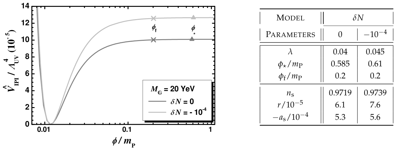
To obtain a first insight for the shape of the inflationary potential in our set-up we plot in Figure 1 ${\widehat{V}}_{\mathrm{IPI}}/{\mathsf{\Lambda }}_{\mathrm{UV}}^4$ in Equation (21a) versus $\varphi$ for $\delta N=0$ (gray line) or $\delta N=-{10}^{-4}$ (light gray line). We take

$$g=0.7, M_{\mathbb{G}}=20 \mathrm{YeV}, c_{\mathcal{R}}=7.25·{10}^3 \mathrm{and} M=28.6 \mathrm{YeV},$$

(39)

where the two latter quantities are obtained consistently with Equations (30) and (17) and we restore units hereafter in this Section for presentation purposes. In both cases we fix ${\widehat{N}}_{★}=52.5$ and arrange the values of some related parameters in the Table of Figure 1. We remark that for both $\delta N$ values ${\widehat{V}}_{\mathrm{IPI}}$ comfortably satisfies Equation (32) and exhibits the same vacuum state (since $c_{\mathcal{R}}$ is the same in both cases). The position of the inflationary plateau, however, is clearly elevated for $\delta N<0$. This means that the corresponding r is larger [125] since $\widehat{ϵ}$ is larger. Indeed, we find that the r value for $\delta N=0$ is less than its value for $\delta N=-{10}^{-4}$. Moreover, $\widehat{\eta }<0$ increases as $\delta N$ decreases and so $n_{\mathrm{s}}$ is lower for $\delta N=0$ as shown in the Table of Figure 1. Indeed, we find $\widehat{\eta }=-0.014$ [$\widehat{\eta }=-0.013$] for $\delta N=0$ [$\delta N=-{10}^{-4}$].

Figure 1. Inflationary potential ${\widehat{V}}_{\mathrm{IPI}}$ in units of ${\mathsf{\Lambda }}_{\mathrm{UV}}$ as a function of $\varphi$ for $\varphi >0$, $g=0.7$, $M_{\mathbb{G}}=20 \mathrm{YeV}$ and $\delta N=0$ (dark gray line) or $\delta N={10}^{-4}$ (light gray line)—the values of ${\varphi }_{★}$ and ${\varphi }_{\mathrm{f}}$ are also indicated. The relevant values of some input and output parameters are listed in the Table—recall that $1 \mathrm{YeV}={10}^{15} \mathrm{GeV}$.

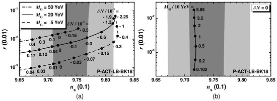
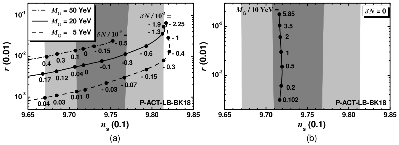
The outputs of our numerical computation are first compared against the P-ACT-LB-BK18 data [2] in the $n_{\mathrm{s}}-r$ plane for $g=0.7$—see Figure 2. In both plots there we depict the marginalized joint $68\%$ and $95\%$ regions from P-ACT-LB-BK18 data by dark and light shaded contours respectively in the background. In Figure 2a we also plot solid, dashed and dot-dashed lines for $M_{\mathbb{G}}=5 \mathrm{YeV}, 20 \mathrm{YeV}$ and $50 \mathrm{YeV}$ correspondingly and show the variation of $\delta N$ along each line. We clearly see that $n_{\mathrm{s}}$ and r increase with $M_{\mathbb{G}}$ and as $\delta N$ decreases. The various lines terminate at large $n_{\mathrm{s}}$ values since the right inequality in Equation (32) is saturated. The variation of $\delta N$ signals a disturbing tuning due to its low magnitude. Indeed we obtain $|dn|<{10}^{-3}$, i.e., three orders of magnitude lower than the corresponding parameter (n) in Ref. [80]. It is worth emphasizing, though, that our proposal assures totally acceptable results without any tuning, i.e., for $\delta N=0$. This is clearly illustrated in Figure 2b, where we display the allowed curve in the $n_{\mathrm{s}}-r$ plane for $N=2$ (i.e, $\delta N=0$) and varying $M_{\mathbb{G}}$ along it. We see that the allowed curve lies well within the 68% c.l. of P-ACT-LB-BK18 data. Also the $M_{\mathbb{G}}$ values include the one favored by the unification of the gauge coupling constants within MSSM, $20 \mathrm{YeV}$. As anticipated below Equation (30), our scheme restricts the allowed $M_{\mathbb{G}}$ (and $c_{\mathcal{R}}$ via Equation (30)) as follows:

$$1.02\lesssim M_{\mathbb{G}}/\mathrm{YeV}\lesssim 58.5, 2.8·{10}^3\gtrsim c_{\mathcal{R}}/{10}^3\gtrsim 8.5 \mathrm{and} 1.45\lesssim M/\mathrm{YeV}\lesssim 83.5$$

(40)

with ${\widehat{N}}_{★}\simeq (52.1-52.9)$, $a_{\mathrm{s}}\simeq -5.3·{10}^{-4}$ and $r\simeq (0.3-18)·{10}^{-5}$. For $M_{\mathbb{G}}$ values lower than the lower bound on $M_{\mathbb{G}}$ in Equation (40) $\lambda$ required by Equation (27) exceeds the perturbative value $3.5$. On the other hand, the upper bound on $M_{\mathbb{G}}$ in Equation (40) comes from the requirement that $\varphi$ has to be kept subplanckian. The obtained $|a_{\mathrm{s}}|$’s remain negligibly small being, thereby, consistent with Equation (1). The contribution of $\mathsf{\Delta }{V}_{\mathrm{I}}$ to ${\widehat{V}}_{\mathrm{IPI}}$ in Equation (24) can be easily eliminated with a suitable selection of $\mathsf{\Lambda }$ as mentioned in Section 3.1. For example, imposing the condition $\mathsf{\Delta }{V}_{\mathrm{I}}\left({\varphi }_{★}\right)=0$, we find ${\mathsf{\Lambda }}_{\mathrm{CW}}\simeq (7.4-56) \mathrm{PeV}$ for the ranges in Equation (40). Under these circumstances, our inflationary predictions can be exclusively reproduced by using ${\widehat{V}}_{\mathrm{IPI}}$ in Equation (21a). If we vary g in the range 0.5–0.9, we obtain some shift of the allowed $M_{\mathbb{G}}$ values whereas the resulting observables remain intact. In particular, for $g=0.5$ we find $0.725\lesssim M_{\mathbb{G}}/\mathrm{YeV}\lesssim 41.5$ whereas for $g=0.9$ we find $1.3\lesssim M_{\mathbb{G}}/\mathrm{YeV}\lesssim 75$.

Figure 2. Allowed curves in the $n_{\mathrm{s}}-r$ plane for $g=0.7$ and (a) various $M_{\mathbb{G}}$’s shown in the legend and varying $\delta N$ as shown along the curves (b) $\delta N=0$ and various $M_{\mathbb{G}}$’s shown along the curve. The marginalized joint $68\%$ [$95\%$] regions from P-ACT-LB-BK18 data are depicted by the dark [light] shaded contours.

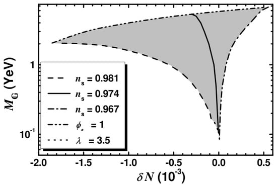
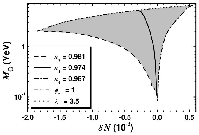
The variation of the observables in Figure 2 reveals that our free parameters can be constrained in the $\delta N-M_{\mathbb{G}}$ plane. The relevant allowed region is shown in Figure 3 for $g=0.7$. It is bounded by (i) the dashed and dot-dashed lines which originate from the upper and the lower bounds on $n_{\mathrm{s}}$ in Equation (1): (ii) the double dot-dashed line along which ${\varphi }_{★}=m_{\mathrm{P}}$ and (iii) the dotted line along which $\lambda =3.5$, i.e., it acquires its maximal possible perturbative value. Fixing $n_{\mathrm{s}}$ to its central value in Equation (1), we obtain the solid line with $\delta N=-(5·{10}^{-2}-3)·{10}^{-4}$ and values for the other parameters very close to those obtained for $\delta N=0$ in Equation (40). Minor changes to the position of the double dot-dashed and dotted curves are expected by varying g in the range 0.5–0.9.

Figure 3. Allowed (shaded) region for $g=0.7$ as determined by Equations (1), (27), (30) and (32) in the $M_{\mathbb{G}}-\delta N$ plane. Along the solid line we fix $n_{\mathrm{s}}=0.974$. The conventions adopted for the various lines are also shown.

4. Post-Inflationary Regime

A byproduct of our inflationary setting is that it assists us to understand the origin of the $\mu$ term of MSSM, as we show in Section 4.2, consistently with the generation of the observable baryon asymmetry—see Section 4.3— if we embed it in a $B-L$ extension of MSSM as detailed in Section 4.1. Our final results are exposed in Section 4.4.

4.1. Set-Up

To achieve the aforementioned $B-L$ extension of MSSM we promote to gauge the pre-existing global $U{\left(1\right)}_{B-L}$—cf. Refs. [77,79]. The supplementary superpotential terms which are relevant for our analysis read

$$\mathsf{\Delta }W={\lambda }_{\mu }S{H}_u{H}_d+h_{ijN}{N}_i^c{L}_j{H}_u+{\lambda }_{i{N}^c}\overline{\mathsf{\Phi }}{N}_i^{c2}.$$

(41a)

On the other hand, $K_2$ in Equation (5) is to be replaced by

$$K_2=N_{\mathrm{st}}ln(1+{\sum }_{a=1}^5{|X_{\alpha }|}^2/N_{\mathrm{st}})$$

(41b)

with $X_{\alpha }=S,{\tilde{N}}_i^c,{\tilde{L}}_j,H_u$ and $H_d$ which parameterizes the compact Kähler manifold $SU\left(15\right)/U\left(1\right)$. Here $H_u$ and $H_d$ are the electroweak Higgs superfields and ${\tilde{N}}_i^c$ and ${\tilde{L}}_j$ are the scalar superpartners of the right-handed neutrinos $N_i^c$ and left-handed leptons $L_j$ respectively with $i=1,2,3$—we work in the basis where ${\lambda }_{i{N}^c}$ is diagonal, real and positive. The charge assignments of $X^{\alpha }$ besides S are

$$(B-L)(L_i,N_i^c,H_u,H_d)=(-1,1,0,0) \mathrm{and} R(L_i,N_i^c,H_u,H_d)=(0,1,0,0).$$

(42)

We assume that $X^{\alpha }$ are stabilized at zero during IPI and so the inflationary trajectory in Equation (20) has to be supplemented by the condition

$${⟨H_u⟩}_{\mathrm{I}}={⟨H_d⟩}_{\mathrm{I}}={⟨{\tilde{N}}_i^c⟩}_{\mathrm{I}}={⟨{\tilde{L}}_j⟩}_{\mathrm{I}}=0.$$

(43)

The consistency of our assumption can be verified by checking the stability of this path. To this end we parameterize the complex fields $X^{\alpha }$ above as S in Equation (19), i.e.,

$$X^{\alpha }=\left(x^{\alpha }+i{\overline{x}}^{\alpha }\right)/\sqrt{2}.$$

(44)

The relevant masses squared are listed in Table 2, where we see that $m_{i{\tilde{\nu }}^c}^2>0$, $m_{i\tilde{l}}^2>0$ and $m_{h+}^2>0$ for any ${\varphi }_{\mathrm{f}}<\varphi <1$—here $m_{h\pm }$ are the eigenvalues associated with the eigenstates of Higgs doublets

$$h_{\pm }=(h_u\pm h_d)/\sqrt{2} \mathrm{and} {\overline{h}}_{\pm }=({\overline{h}}_u\pm {\overline{h}}_d)/\sqrt{2}.$$

(45)

Table 2. Mass-squared spectrum of the non-inflaton sector along the path in Equations (20) and (43).

Fields	Eigenstates	Masses Squared
26 Real	$h_{\pm },{\overline{h}}_{\pm }$	$m_{h\pm }^2$	$3\left(1+1/N_{\mathrm{st}}\pm 4{\lambda }_{\mu }{c}_{\mathcal{R}}/\lambda f_{\mathrm{W}}\right){\widehat{H}}_{\mathrm{IPI}}^2$
Scalars	${\tilde{\nu }}_i^c,{\overline{\tilde{\nu }}}_i^c$	$m_{i{\tilde{\nu }}^c}^2$	$3\left(1+1/N_{\mathrm{st}}+16{\lambda }_{i{N}^c}^2/{\lambda }^2{\varphi }^2\right){\widehat{H}}_{\mathrm{IPI}}^2$
	${\tilde{l}}_i,{\overline{\tilde{l}}}_i$	$m_{i\tilde{l}}^2$	$3(1+1/N_{\mathrm{st}}){\widehat{H}}_{\mathrm{IPI}}^2$
3 Weyl Spinors	$N_i^c$	$M_{i{N}^c}^2$	$48{\lambda }_{i{N}^c}^2{c}_{\mathcal{R}}^2{\varphi }^2{\widehat{H}}_{\mathrm{IPI}}^2/{\lambda }^2{f}_{\mathrm{W}}^2$

Note that $m_s$ remains as shown in Table 1. On the other hand, the positivity of $m_{h-}^2$ dictates the establishment of the inequality—cf. Refs. [45,79]:

$${\lambda }_{\mu }<\lambda (1+N_{\mathrm{st}})(c_{\mathcal{R}}{\varphi }_{\mathrm{f}}^2-1)/4N_{\mathrm{st}}{c}_{\mathcal{R}} \Rightarrow {\lambda }_{\mu }/\lambda <(1+1/N_{\mathrm{st}}){\varphi }_{\mathrm{f}}^2/4,$$

(46)

where ${\varphi }_{\mathrm{f}}$ is given by Equation (34). e.g., for the ranges of parameters in Equation (40) we obtain $0.001\lesssim {\lambda }_{\mu }/\lambda \lesssim 0.06$. Due to the extra contributions of Table 2 the total radiative correction to ${\widehat{V}}_{\mathrm{IPI}}$ in Equation (21a) now becomes

$$\mathsf{\Delta }{V}_{\mathrm{tot}}=\mathsf{\Delta }{V}_{\mathrm{I}}+\mathsf{\Delta }{V}_{\mathrm{pI}}$$

(47)

where $\mathsf{\Delta }{V}_{\mathrm{I}}$ is given by Equation (24), whereas the latter term takes the form

$$\mathsf{\Delta }{V}_{\mathrm{pI}}={\displaystyle \frac{1}{64{\pi }^2}}\left(\sum _{\alpha }{\mathrm{N}}_{\alpha }{m}_{\alpha }^{4}ln{\displaystyle \frac{m_{\alpha }^2}{{\mathsf{\Lambda }}_{\mathrm{CW}}^2}}-6M_{i{N}^c}^{4}ln{\displaystyle \frac{M_{i{N}^c}^2}{{\mathsf{\Lambda }}_{\mathrm{CW}}^2}}\right) \mathrm{where} \left\{\begin{array}{cc}\alpha \hfill & =\{h\pm ,i{\tilde{\nu }}^c,i\tilde{l}\}\hfill \\ {\mathrm{N}}_{\alpha }\hfill & =\{8,6,12\}\hfill \end{array}\right..$$

(48)

As a consequence, ${\mathsf{\Lambda }}_{\mathrm{CW}}$ should be readjusted if we impose the condition $\mathsf{\Delta }{V}_{\mathrm{tot}}\left({\varphi }_{★}\right)=0$. e.g., for the ranges of parameters in Equation (40) we find ${\mathsf{\Lambda }}_{\mathrm{CW}}\simeq (0.77-5.85) \mathrm{ZeV}$; hereafter, we restore units.

4.2. Generation of the $\mu$ Term of MSSM

The contributions from the soft SUSY-breaking terms, although negligible during IPI—since these are much smaller than $\varphi \sim m_{\mathrm{P}}$—may shift slightly $⟨S⟩$ from zero in Equation (17). Indeed, the relevant potential terms are

$$V_{\mathrm{soft}}=\left(\lambda A_{\lambda }S\overline{\mathsf{\Phi }}\mathsf{\Phi }+{\lambda }_{\mu }{A}_{\mu }S{H}_u{H}_d+{\lambda }_{i{N}^c}{A}_{i{N}^c}\mathsf{\Phi }{\tilde{N}}_i^{c2}-{\mathrm{a}}_{S}S\lambda M^2/4+\mathrm{h}.\mathrm{c}.\right)+m_{\alpha }^2{\left|X^{\alpha }\right|}^2,$$

(49)

where $m_{\alpha },A_{\lambda },A_{\mu },A_{i{N}^c}$ and ${\mathrm{a}}_S$ are soft SUSY-breaking mass parameters. Rotating S in the real axis by an appropriate R transformation, choosing conveniently the phases of $A_{\lambda }$ and ${\mathrm{a}}_S$ so as the total low energy potential $V_{\mathrm{tot}}=V_{\mathrm{SUSY}}+V_{\mathrm{soft}}$ to be minimized—see Equation (16)—and substituting $H_u=H_d=0$ and $\mathsf{\Phi }=\overline{\mathsf{\Phi }}=M/2$ from Equation (17) we get

$$⟨V_{\mathrm{tot}}\left(S\right)⟩={\displaystyle \frac{1}{2}}{\lambda }^2{M}^2{S}^2-\lambda M^{2}S{\mathrm{a}}_{\mu }{m}_{3/2} \mathrm{with} {\mathrm{a}}_{\mu }=\left(|A_{\lambda }|+|{\mathrm{a}}_S|\right)/2m_{3/2},$$

(50a)

where $m_{3/2}$ is the $\tilde{G}$ (gravitino) mass and ${\mathrm{a}}_{\mu }>0$ is a parameter of order unity which parameterizes our ignorance for the dependence of $|A_{\lambda }|$ and $|{\mathrm{a}}_S|$ on $m_{3/2}$. We also take into account that $m_S\ll M$. The extermination condition for $⟨V_{\mathrm{tot}}\left(S\right)⟩$ w.r.t S leads to a non vanishing $⟨S⟩$ as follows

$$d⟨V_{\mathrm{tot}}\left(S\right)⟩/dS=0 \Rightarrow ⟨S⟩\simeq {\mathrm{a}}_{\mu }{m}_{3/2}/\lambda ,$$

(50b)

The extremum above is a global minimum since $d^2⟨V_{\mathrm{tot}}\left(S\right)⟩/d{S}^2={\lambda }^2{M}^2>0$. The SUSY breaking effects, considered in Equation (49), explicitly break $U{\left(1\right)}_R$ to the subgroup ${\mathbb{Z}}_2^R$, which remains unbroken by $⟨S⟩$ in Equation (50b) and so no disastrous domain walls are formed.

The generated $\mu$ parameter from the first term in Equation (41a) is

$$\mu ={\lambda }_{\mu }⟨S⟩\simeq {\lambda }_{\mu }{\mathrm{a}}_{\mu }{m}_{3/2}/\lambda .$$

(51)

This results reveals that $\mu /m_{3/2}$ follows the behavior of the ratio ${\lambda }_{\mu }/\lambda$ shown below Equation (46). The emerged hierarchy between $\mu$ and $m_{3/2}$ is mildly stronger than that obtained in Refs. [45,77,80,81,95], rendering our present setting apparently distinguishable from those. Namely, our present result hints at split SUSY [108,109], where the soft SUSY scalar mass parameters—therefore, the SUSY mass scale, $\tilde{m}$—are expected to lie at an intermediate mass scale whereas $\mu$ and the gaugino masses can be kept of the order of TeV. As a consequence, the candidacy of the lightest SUSY particle (LSP)—which is normally the lightest neutralino, $\tilde{\chi }$—as cold dark matter (CDM) particle remains possible and the gauge coupling unification is still valid for g and $M_{\mathbb{G}}$ values similar to those used in the conventional MSSM.

Given that the LEP bound on the mass of charginos [126] dictates $\mu >0.1 \mathrm{TeV}$, Equation (51) consistently with Equations (36) and (30) favors $m_{3/2}>1 \mathrm{PeV}$. On the other hand, if $\tilde{m}$ is identified with $m_{3/2}$, our proposal can be probed via the measured value of the Higgs boson mass [127,128]. Within split SUSY, updated analysis requires [110]

$$10 \mathrm{TeV}\lesssim m_{3/2}\lesssim 60 \mathrm{PeV},$$

(52)

for degenerate sparticle spectrum and varying $tan\beta$ and stop mixing. The lower bound above is moved up to $20 \mathrm{PeV}$ for low $tan\beta$ values and minimal stop mixing. The upper bound above can be moved up to $100 \mathrm{PeV}$ for scalar mass parameters larger or smaller than $m_{3/2}$ by a factor of 3. Note that the upper bound on Equation (52) automatically renders the gluino with mass of order $1 \mathrm{TeV}$ cosmologically safe [129].

4.3. Non-Thermal Leptogenesis After IPI

Besides the generation of the $\mu$ term, $\mathsf{\Delta }W$ in Equation (41a) allows for the implementation of nTL via the direct decay of the inflaton into $N_i^c$—see Section 4.3.1. For the success of this process, however, one has to produce the correct baryon asymmetry—see Section 4.3.2—and circumvent the $\tilde{G}$ overproduction problem as discussed in Section 4.3.3.

4.3.1. Inflaton Mass and Decay

Soon after the end of IPI, we obtain a very short period of OI—see Appendix A—which is followed by the usual phase of damped oscillations abound the minimum in Equation (17) where the (canonically normalized) inflaton $\delta \varphi =\varphi -M$ acquires mass

$$m_{\delta \varphi }={⟨{\widehat{V}}_{\mathrm{IPI},\varphi \varphi }⟩}^{1/2}=\lambda m_{\mathrm{P}}/\sqrt{2c_{\mathcal{R}}},$$

(53)

which ranges in the interval $(4.76-36)·{10}^{-1} \mathrm{YeV}$ with decreasing $M_{\mathbb{G}}$ (or increasing $c_{\mathcal{R}}$). Note that it does not depend on N (and $\delta N$) thanks to the canonical normalization of $\delta \varphi$. This oscillatory period terminates at the moment of reheating where the temperature of the universe acquires the value [45]

$$T_{\mathrm{rh}}={\left(72/5{\pi }^2{g}_{*}\right)}^{1/4}{\left({\mathsf{\Gamma }}_{\delta \varphi }{m}_{\mathrm{P}}\right)}^{1/2} \mathrm{with} {\mathsf{\Gamma }}_{\delta \varphi }={\mathsf{\Gamma }}_{\delta \varphi \to N_i^c}+{\mathsf{\Gamma }}_{\delta \varphi \to H}+{\mathsf{\Gamma }}_{\delta \varphi \to XYZ},$$

(54)

where $g_{*}=228.75$ counts the MSSM effective number of relativistic degrees of freedom and we take into account the following decay widths

$$\begin{array}{ccc}\hfill {\mathsf{\Gamma }}_{\delta \varphi \to N_i^c}& =& {\displaystyle \frac{g_{i{N}^c}^2}{16\pi }}{m}_{\delta \varphi }{\left(1-4{M_{i{N}^c}^2}^2/m_{\delta \varphi }^2\right)}^{3/2} \mathrm{with} g_{i{N}^c}=(N-1){\lambda }_{i{N}^c};\hfill \end{array}$$

(55a)

$$\begin{array}{ccc}\hfill {\mathsf{\Gamma }}_{\delta \varphi \to H}& =& {\displaystyle \frac{2}{8\pi }}{g}_H^2{m}_{\delta \varphi } \mathrm{with} g_H={\lambda }_{\mu }/\sqrt{2};\hfill \end{array}$$

(55b)

$$\begin{array}{ccc}\hfill {\mathsf{\Gamma }}_{\delta \varphi \to XYZ}& =& {\displaystyle \frac{14g_y^2}{512{\pi }^3}}{\displaystyle \frac{m_{\delta \varphi }^3}{m_{\mathrm{P}}^2}} \mathrm{with} g_y=y_{3}N{c}_{\mathcal{R}}^{1/2}.\hfill \end{array}$$

(55c)

Here $y_3=h_{t,b,\tau }\left(m_{\delta \varphi }\right)\simeq 0.5$ with $h_t,h_b$ and $h_{\tau }$ being the Yukawa coupling constants; we assume that diagonalization has been performed in the generation space. The various decay widths above arise from the respective lagrangian terms

$$\begin{array}{ccc}\hfill {\mathcal{L}}_{\delta \varphi \to N_i^c{N}_i^c}& =& -{\displaystyle \frac{1}{2}}{e}^{K/2m_{\mathrm{P}}^2}\mathsf{\Delta }{W}_{,N_i^c{N}_i^c}{N}_i^c{N}_i^c+\mathrm{h}.\mathrm{c}.=g_{i{N}^c}\delta \varphi \left(N_i^c{N}_i^c+\mathrm{h}.\mathrm{c}.\right)+\dots ,\hfill \end{array}$$

(56a)

$$\begin{array}{ccc}\hfill {\mathcal{L}}_{\delta \varphi \to H_u{H}_d}& =& -e^{K/m_{\mathrm{P}}^2}{K}^{S{S}^{*}}{\left|\mathsf{\Delta }{W}_{,S}\right|}^2=-g_H{m}_{\delta \varphi }\delta \varphi \left(H_u^{*}{H}_d^{*}+\mathrm{h}.\mathrm{c}.\right)+\dots ,\hfill \end{array}$$

(56b)

$$\begin{array}{ccc}\hfill {\mathcal{L}}_{\delta \varphi \to XYZ}& =& g_y(\delta \varphi /m_{\mathrm{P}})\left(X{\psi }_Y{\psi }_Z+Y{\psi }_X{\psi }_Z+Z{\psi }_X{\psi }_Y+\mathrm{h}.\mathrm{c}.\right),\hfill \end{array}$$

(56c)

describing $\delta \varphi$ decay into a pair of $N_j^c$ with masses $M_{j{N}^c}={\lambda }_{j{N}^c}M$, $H_u$ and $H_d$ and three MSSM (s)-particles $X,Y$ and Z, respectively. We remark that $g_y$ is proportional to $c_{\mathcal{R}}^{1/2}$ and therefore it is rather enhanced due to the large $c_{\mathcal{R}}$ values employed in our scheme—see, e.g., Equation (40).

4.3.2. Baryon-Number Abundance

For $T_{\mathrm{rh}}<M_{i{N}^c}$, the out-of-equilibrium decay of $N_i^c$ generates a lepton-number asymmetry (per $N_i^c$ decay), ${\epsilon }_i$. The resulting lepton-number asymmetry is partially converted through sphaleron effects into a yield of the observed baryon asymmetry of the universe

$$Y_B=-0.35·{\displaystyle \frac{5}{4}}{\displaystyle \frac{T_{\mathrm{rh}}}{m_{\delta \varphi }}}\sum _i{\displaystyle \frac{{\mathsf{\Gamma }}_{\delta \varphi \to N_i^c}}{{\mathsf{\Gamma }}_{\delta \varphi }}}{\epsilon }_i,$$

(57)

where the quantity ${\epsilon }_i$ can be expressed in terms of the Dirac masses of ${\nu }_i$, $m_{i\mathrm{D}}$, arising from the second term of Equation (41a)—see Ref. [77]. Moreover, employing the type I seesaw formula we can then obtain the light-neutrino mass matrix $m_{\nu }$ in terms of $m_{i\mathrm{D}}$ and $M_{i{N}^c}$. As a consequence, nTL can be nicely linked to low energy neutrino data. We take as inputs the recently updated best-fit values [130]—cf. Ref. [77]—on the neutrino oscillation parameters including IceCube IC24 with Super Kamiokande (SK) atmospheric data. We consider only the scheme of normal ordered neutrino masses, $m_{i\nu }$’s, which can become consistent with the upper bound on the sum of $m_{i\nu }$’s

$$\sum _i{m}_{i\nu }\le 0.082 \mathrm{eV},$$

(58)

induced from P-ACT-LB data [1] at 95% c.l. Namely, we take [130] $\mathsf{\Delta }{m}_{21}^2=7.49·{10}^{-5} {\mathrm{eV}}^2$ and $\mathsf{\Delta }{m}_{31}^2=2.513·{10}^{-3} {\mathrm{eV}}^2$ for the mass-squared differences, ${sin}^2{\theta }_{12}=0.308$, ${sin}^2{\theta }_{13}=0.02215$ and ${sin}^2{\theta }_{23}=0.47$ for the mixing angles, and $\delta =1.1788\pi$ for the CP-violating Dirac phase.

The validity of Equation (57) requires that the $\delta \varphi$ decay into a pair of $N_i^c$’s is kinematically allowed for at least one species of the $N_i^c$’s and also that there is no erasure of the produced lepton yield due to $N_1^c$ mediated inverse decays and $\mathsf{\Delta }L=1$ scatterings. These prerequisites are ensured if we impose

$$10T_{\mathrm{rh}}\lesssim M_{1N^c}\le m_{\delta \varphi }/2.$$

(59)

Finally, Equation (57) has to reproduce the observational result [1]

$$Y_B=\left(8.75\pm 0.085\right)·{10}^{-11} \Rightarrow 8.665\lesssim Y_B/{10}^{-11}\lesssim 8.835.$$

(60)

4.3.3. Gravitino Abundance

The required $T_{\mathrm{rh}}$ in Equation (57) must be compatible with constraints on the $\tilde{G}$ abundance, $Y_{3/2}$, at the onset of nucleosynthesis (BBN), which is estimated to be [105,106,107]

$$Y_{3/2}\simeq 1.9·{10}^{-13}{T}_{\mathrm{rh}}/\mathrm{EeV},$$

(61)

where we assume that $\tilde{G}$ decays with a tiny hadronic branching ratio and take into account only thermal production of $\tilde{G}$, and assume that $\tilde{G}$ is much heavier than the MSSM gauginos. Non-thermal contributions to $Y_{3/2}$ [131] are also possible but strongly dependent on the mechanism of soft SUSY breaking. It is notable, though, that these contributions to $Y_{3/2}$ in models with stabilizer field, as in our case, are significantly suppressed compared to the thermal ones [132].

On the other hand, $Y_{3/2}$ is bounded from above in order to avoid spoiling the success of the BBN. The corresponding bounds result to upper bounds on $T_{\mathrm{rh}}$—cf. Ref. [45]—which are violated in our case since the achievement of the correct $Y_B$ requires $T_{\mathrm{rh}}>10 \mathrm{EeV}$ as we see in Table 3. We are obliged, therefore, to adopt one of the following two alternative scenarios:

Table 3. Parameters yielding the correct $Y_B$ in Equation (60) for various neutrino masses. We take $g=0.7$ $M_{\mathbb{G}}=20 \mathrm{YeV}$, $N=2N_{\mathrm{st}}=2$ $m_{3/2}=40 \mathrm{PeV}$ and ${\lambda }_{\mu }={10}^{-6}$—recall that $1 \mathrm{ZeV}={10}^{-3} \mathrm{YeV}={10}^{12} \mathrm{GeV}$.

Parameters	Cases
	A	B	C	D	E	F	G	H
Low Scale Parameters
$m_{1\nu }/0.001 \mathrm{eV}$	$0.1$	$0.79$	$0.869$	1	1	2	$9.9$	10
$m_{2\nu }/0.001 \mathrm{eV}$	$8.6$	$8.7$	$8.7$	$8.7$	$8.7$	$8.8$	$13.1$	$13.2$
$m_{3\nu }/0.01 \mathrm{eV}$	5	5	5	5	5	5	$5.1$	$5.1$
${\sum }_i{m}_{i\nu }/0.01 \mathrm{eV}$	$5.88$	$5.96$	$5.98$	$5.98$	$5.9$	$6.1$	$7.41$	$7.43$
${\phi }_1$	$\pi /20$	0	$-\pi /3$	0	$\pi /7$	0	$\pi /10$	0
${\phi }_2$	0	$-\pi$	$2\pi$	$\pi /25$	$-2\pi$	$-\pi /15$	0	0
Leptogenesis-Scale Parameters
$m_{1\mathrm{D}}/1 \mathrm{GeV}$	$93.8$	$79.81$	$86.3$	$89.6$	$11.1$	77	116	$120.1$
$m_{2\mathrm{D}}/1 \mathrm{GeV}$	$70.1$	60	$95.98$	$89.6$	$130.67$	$120.44$	$80.595$	121
$m_{3\mathrm{D}}/1 \mathrm{GeV}$	$169.46$	111	100	90	160	200	$99.9$	$141.38$
$M_{1N^c}/0.1 \mathrm{YeV}$	$1.63$	$1.34$	$1.9$	$1.61$	$4.06$	$4.05$	$1.68$	$3.3$
$M_{2N^c}/1 \mathrm{YeV}$	$1.4$	$0.88$	1	$0.2$	$1.9$	$1.17$	$0.69$	$1.8$
$M_{3N^c}/1 \mathrm{YeV}$	126	$11.2$	$8.45$	8	$15.8$	$8.12$	$1.8$	$1.6$
Branching Ratio for $\delta \varphi$ Decay into $N_1^c$’s
${\mathsf{\Gamma }}_{\delta \varphi \to N_1^c}/{\mathsf{\Gamma }}_{\delta \varphi } (\%)$	41	$33.9$	$46.1$	$40.6$	$7.7·{10}^{-3}$	$0.29$	38	42
Resulting $T_{\mathrm{rh}}$
$T_{\mathrm{rh}}/10 \mathrm{ZeV}$	$1.4$	$1.3$	$1.44$	$1.37$	$1.06$	$1.06$	$1.46$	$1.39$
Resulting B-Yield
$Y_B/{10}^{-11}$	$8.83$	$8.83$	$8.75$	$8.71$	$8.76$	$8.83$	$8.83$	$8.82$

(a)

Short-lived $\tilde{G}$

In this scenario, $\tilde{G}$ decays before BBN—but after LSP freeze-out—and so, the BBN bounds on $T_{\mathrm{rh}}$ no longer apply. To accommodate this situation we compute the $\tilde{G}$ decay temperature $T_{3/2}$ obtained by the condition $H\left(T_{3/2}\right)\simeq {\mathsf{\Gamma }}_{3/2}$ where ${\mathsf{\Gamma }}_{3/2}$ is the decay width of $\tilde{G}$. We find

$$T_{3/2}={\left(90/{\pi }^2{g}_{\mathrm{SM}\ast }\right)}^{1/4}{\left({\mathsf{\Gamma }}_{3/2}{m}_{\mathrm{P}}\right)}^{1/2} \mathrm{where} {\mathsf{\Gamma }}_{3/2}={\displaystyle \frac{1}{32\pi }}\left({\displaystyle \frac{1}{3}}{N}_{\mathrm{ch}}+N_{\mathrm{gs}}\right){\displaystyle \frac{m_{3/2}^3}{m_{\mathrm{P}}^2}}$$

(62)

is estimated taking the large $\tilde{G}$ mass limit with $N_{\mathrm{ch}}=49$ and $N_{\mathrm{gs}}=12$ being [133] the number of chiral superfields (neglecting $N_i^c$’s) and the number of gauginos in the MSSM respectively. Also $g_{\mathrm{SM}\ast }=106.75$ is the effective number of the relativistic degrees of freedom of the Standard Model. Requiring that $T_{3/2}$ is larger than the temperature at the commencement of BBN, $T_{\mathrm{BBN}}\simeq 2 \mathrm{MeV}$ we obtain the lower bound on $m_{3/2}$, $m_{3/2}>50 \mathrm{TeV}$. On the other hand, the abundance of the neutralino, $\tilde{\chi }$, LSP obtained by the $\tilde{G}$ decay is estimated to be

$${\mathsf{\Omega }}_{\tilde{\chi }}{h}^2=2.75·{10}^{11}{Y}_{3/2}{m}_{\tilde{\chi }}/1 \mathrm{TeV},$$

(63)

where $Y_{3/2}$ is given by Equation (61)—$\mathsf{\Omega }$ here should not be confused with the frame function in Equation (12a). The resulting ${\mathsf{\Omega }}_{\tilde{\chi }}{h}^2$ should be consistent with upper bound from the CDM considerations [1] which provides us with an upper bound on $m_{\tilde{\chi }}$ as follows

$${\mathsf{\Omega }}_{\tilde{\chi }}{h}^2\lesssim 0.12 \stackrel{\left(63\right)}{⟹} m_{\tilde{\chi }}/1 \mathrm{TeV}\gtrsim 2.3\left(1 \mathrm{EeV}/T_{\mathrm{rh}}\right).$$

(64)

According to the updated results in Ref. [134] a lower bound on $m_{\tilde{\chi }}$ can be inferred by imposing a number of cosmo-phenomenological requirements which can be translated to an upper bound on $T_{\mathrm{rh}}$ via Equation (64). In particular,

$$m_{\tilde{\chi }}\gtrsim 40 \mathrm{GeV} \stackrel{\left(64\right)}{⟹} T_{\mathrm{rh}}\lesssim 57 \mathrm{EeV},$$

(65)

which is slightly higher than the upper bounds on $T_{\mathrm{rh}}$ obtained in the case of the long-lived $\tilde{G}$ [106]—cf. Refs. [45,77,98]. This relaxation is not enough for our purposes as we see in Section 4.4.

(b)

Very short-lived $\tilde{G}$

This scenario allows for $T_{\mathrm{rh}}$ values higher than that in Equation (65). According to it, $\tilde{G}$ decays before the freeze-out process of $\tilde{\chi }$ LSP which takes place for temperature $T_{\mathrm{fo}}=x_{\mathrm{fo}}{m}_{\tilde{\chi }}>T_{\mathrm{BBN}}$ with $x_{\mathrm{fo}}=1/25-1/20$. To achieve this we demand

$$T_{3/2}>T_{\mathrm{fo}} \stackrel{\left(62\right)}{⟹} m_{3/2}>2^{3/2}{\left({\displaystyle \frac{g_{\mathrm{SM}\ast }}{5}}\right)}^{1/6}{\left({\displaystyle \frac{m_{\mathrm{P}}{\left(\pi x_{\mathrm{fo}}{m}_{\tilde{\chi }}\right)}^2}{N_{\mathrm{ch}}+3N_{\mathrm{gs}}}}\right)}^{1/3},$$

(66)

which can be translated numerically as

$$m_{3/2}>3.1 \mathrm{PeV}{(x_{\mathrm{fo}}{m}_{\tilde{\chi }}/1 \mathrm{GeV})}^{2/3}.$$

(67)

e.g., for $m_{\tilde{\chi }}=1 \mathrm{TeV}$ we obtain $m_{3/2}>36 \mathrm{PeV}$ [$m_{3/2}>42 \mathrm{PeV}$] with $x_{\mathrm{fo}}=1/25$ [$x_{\mathrm{fo}}=1/20$] which lies inside the region of Equation (52), whose the upper bound requires $m_{\tilde{\chi }}\lesssim 2.15 \mathrm{TeV}$ [$m_{\tilde{\chi }}\lesssim 1.7 \mathrm{TeV}$] for $x_{\mathrm{fo}}=1/25$ [$x_{\mathrm{fo}}=1/20$].

4.4. Results

The numerical implementation of our post-inflationary setting can be processed following the bottom-up approach detailed in Ref. [77]. Namely, we find the $M_{i{N}^c}$’s using as inputs the $m_{i\mathrm{D}}$’s, $m_{1\nu }$, the two Majorana phases ${\phi }_1$ and ${\phi }_2$ of the PMNS matrix, and the best-fit values of the neutrino oscillation parameters, mentioned in Section 4.3. Since the gauge group adopted here, ${\mathbb{G}}_{B-L}$, no specific relation is predicted between the Yukawa couplings constants $h_{iN}$ entering the second term of Equation (41a) and the other Yukawa couplings in the MSSM. As a consequence, the $m_{i\mathrm{D}}$’s are free parameters. However, for the sake of comparison, for cases B, C, D and G we take $m_{3\mathrm{D}}=m_t\simeq 100 \mathrm{GeV}$, where $m_t$ denotes the mass of the top quark estimated at a scale close to $m_{\delta \varphi }$ in Equation (53), i.e., $0.1 \mathrm{YeV}$.

Throughout our computation we take the values of parameters in Equation (39) and $\delta N=0$—see Table in Figure 1. For these inputs we obtain $m_{\delta \varphi }=0.8\mathrm{YeV}$, independently of $\delta N$, and ${\mathsf{\Lambda }}_{\mathrm{CW}}\simeq 3.4 \mathrm{ZeV}$. Also, we select $N_{\mathrm{st}}=1$, $\mu =1 \mathrm{TeV}$ (with soft SUSY-breaking masses for the gauginos of the same order of magnitude) and $m_{3/2}=40 \mathrm{PeV}$ which fulfils Equation (67). As a result we have ${\lambda }_{\mu }={10}^{-6}$ which is consistent with Equation (46). Finally, we take $y=0.5$ in Equation (55c), which is a typical value encountered for various MSSM settings.

In Table 3 we present eight benchmark points with increasing $m_{1\nu }$’s, where all the restrictions of Section 4.3, together with those from Equations (1), (27), (30) and (32), can be met. From our computation, we remark the following:

(i)

${\mathsf{\Gamma }}_{\delta \varphi \to H}$ turns out to be much less than ${\mathsf{\Gamma }}_{\delta \varphi \to XYZ}$ and ${\mathsf{\Gamma }}_{\delta \varphi \to N_i^c}$ which yield the dominant contributions into ${\mathsf{\Gamma }}_{\delta \varphi }$—similar hierarchy emerges also in Refs. [80,81]. As a consequence, the precise value of $\mu /m_{3/2}$ which influences ${\mathsf{\Gamma }}_{\delta \varphi \to H}$ is not so crucial for the compatibility with Equation (60)—contrary to what happens in Ref. [45].

(ii)

$\delta \varphi$ exclusively decays into the lightest of $N_i^c$’s, $N_1^c$ since the upped bound of Equation (59) is violated for the other $N_i^c$’s.

(iii)

Due to the large values of ${\mathsf{\Gamma }}_{\delta \varphi \to XYZ}$ and ${\mathsf{\Gamma }}_{\delta \varphi \to N_i^c}$, $T_{\mathrm{rh}}$ turns out to be above $10 \mathrm{PeV}$ and so, the standard scenario of the long-lived $\tilde{G}$ and that of short-lived $\tilde{G}$ do not work. However, our results are perfectly acceptable for a very short-lived $\tilde{G}$ with $m_{3/2}\ge 40 \mathrm{PeV}$ and $m_{\tilde{\chi }}\sim 1 \mathrm{TeV}$ as mentioned below Equation (67).

(iv)

The maximal value of $|{\epsilon }_1|$ turns out to be larger than its required value by Equation (60) and for this reason $M_{1N^c}$ has to be confined close to its lower bound in Equation (59) in cases A, B, C, D and G or close to the upper bound of Equation (59) in cases E and F in order to decrease $|{\epsilon }_1|$ to an acceptable level. This adjustment is accommodated by selecting appropriately $m_{i\mathrm{D}}$’s and the Majorana phases for any chosen $m_{1\nu }$. Possible incorporation of wash-out effects [135] could offer a larger flexibility in the exploration of the available parameter space.

Let us comment, finally, on the variation of the fixed values of parameters in our sample cases in Table 3. Varying $\delta N$ is expected to cause a minor impact on our results due to its tiny allowed magnitude—see Figure 3—and the independence of $m_{\delta \varphi }$ from it. On the other hand, changing $M_{\mathbb{G}}$ we expect that the various neutrino parameters in Table 3 have to be carefully readjusted in order to reproduce the correct $Y_B$. No dramatic changes of the $T_{\mathrm{rh}}$ and $M_{i{N}^c}$ values are expected.

The large $T_{\mathrm{rh}}$ values needed in our scheme is undoubtedly a somehow troublesome feature of our post-inflationary scenario. This effect can be partially avoided, if we consider lower $M_{i{N}^c}$ values. In a such case, the explanation of the neutrino masses via the type I seesaw mechanism will remain valid but the leptogenesis will be inadequate. Other baryogenesis mechanisms, such as Affleck-Dine [136] or soft [137] leptogenesis can be alternatively activated then.

5. Conclusions

We retrofitted our proposal in Refs. [80,81] to obtain ample consistency with the recent ACT DR6 extending one of the models constructed in Ref. [24]. Namely, our model is inspired by the Palatini gravity and admits a realization within standard SUGRA adopting the super- and Kähler potentials W and K in Equations (2) and (4) which lead to the inflationary potential in Equation (21a) with canonical kinetic term—cf. Ref. [82]. The free parameters of this potential $(\lambda ,M,c_{\mathcal{R}},N)$ are constrained at the vacuum of the theory imposing the IG and gauge coupling-unification conditions in Equations (18) and (30) besides the inflationary constraints in Equation (27). The aforementioned requirements influenced via $M_{\mathbb{G}}$ in Equation (30) our inflationary scenario and via the strong decay width in Equation (55c) our post-inflationary scenario.

The model naturally predicts $(n_{\mathrm{s}},r)$ values within the $1-\sigma$ margin of ACT DR6 as shown in Figure 2b without any tuning and constraining the allowed margin of $M_{\mathbb{G}}$ to values around the “sweet” spot predicted by the gauge unification within MSSM—see Equation (40). As a consequence, our present framework drastically reduces the allowed parameter space found for a gauge-singlet inflaton with quartic potential in Ref. [24]. We also specified a post-inflationary completion, based on the extra W terms in Equation (41a) and $K_2$ in Equation (41b), which favors split SUSY with $m_{3/2}\simeq (40-60) \mathrm{PeV}$ and allows for baryogenesis via nTL with $T_{\mathrm{rh}}$ of the order of $10 \mathrm{ZeV}$. The problems with the $\tilde{G}$ cosmology are surpassed by arranging $\tilde{G}$ to decay before the freeze-out of the neutralino LSP with mass $m_{\tilde{\chi }}\le 2 \mathrm{TeV}$. In the context of split SUSY the relevant $m_{3/2}$ range (which is considered identical with the SUSY mass scale $\tilde{m}$) is consistent with the Higgs boson mass discovered in LHC.

Appendix A.1. Equation of Motion

To check if the period of OI [111,112] has a sizable impact on the post-inflationary era, we solve numerically the relevant equation of motion for the inflaton $\varphi$. In particular, the cosmological evolution of $\varphi$ in the EF is governed by the following equation—see, e.g., Ref. [124]:

$$\ddot{\varphi }+3\widehat{H}\dot{\varphi }+{\widehat{V}}_{\mathrm{IPI},\varphi }=0$$

(A1)

where dot denotes derivation w.r.t. the cosmic time t, $\widehat{H}$ is the Hubble parameter in the EF and ${\widehat{V}}_{\mathrm{IPI}}$ is given in Equation (21a). In Equation (A1), we neglect the damping term ${\mathsf{\Gamma }}_{\delta \varphi }\dot{\varphi }$ which is important only at the final stage of rapid oscillations of $\varphi$ near the minimum of ${\widehat{V}}_{\mathrm{IPI}}$ [123].

The solution of Equation (A1) can be facilitated, if we use as independent variable the (total) number of e-foldings $\mathsf{\tau }$ defined by

$$\mathsf{\tau }=ln\widehat{R}/{\widehat{R}}_{\mathrm{i}} \Rightarrow \dot{\mathsf{\tau }}=\widehat{H} \mathrm{and} \dot{\widehat{H}}={\widehat{H}}^{\prime }\widehat{H}.$$

(A2)

Here the prime denotes derivation w.r.t. $\mathsf{\tau },\widehat{R}\left(t\right)$ is the EF scale factor and ${\widehat{R}}_{\mathrm{i}}$ is its value at the commencement of IPI, which turns out to be numerically irrelevant. Converting the time derivatives to derivatives w.r.t. $\mathsf{\tau }$, Equation (A1) is equivalent to the following system of two first order equations

$$F_{\varphi }=\widehat{H}{\widehat{R}}^3{\varphi }^{\prime } \mathrm{and} \widehat{H}{F}_{\varphi }^{\prime }=-{\widehat{V}}_{\mathrm{IPI},\varphi }{\widehat{R}}^3 \mathrm{with} F_{\varphi }=\dot{\varphi }{\widehat{R}}^3.$$

(A3)

This system can be solved numerically by taking

$$\widehat{H}=\sqrt{{\displaystyle \frac{{\rho }_{\varphi }}{3m_{\mathrm{P}}^2}}} \mathrm{with} {\rho }_{\varphi }={\displaystyle \frac{1}{2}}{\dot{\varphi }}^2+{\widehat{V}}_{\mathrm{IPI}}={\displaystyle \frac{F_{\varphi }^2}{2{\widehat{R}}^6}}+{\widehat{V}}_{\mathrm{IPI}}$$

(A4)

the energy density of $\varphi$ during and after IPI. To resolve Equation (A3) we impose the initial conditions (at $\mathsf{\tau }=0$) $\varphi \left(0\right)=(0.5-1)m_{\mathrm{P}}$ and ${\varphi }^{\prime }\left(0\right)=0$. We checked that our results are pretty stable against variation of $\varphi \left(0\right)$.

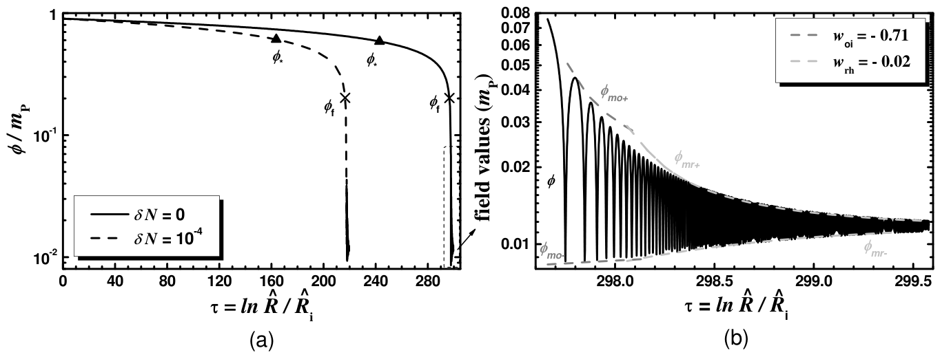
To gain a deeper understanding of the $\varphi$ evolution during and after IPI, we plot in Figure A1a the evolution of $\varphi$ as a function of $\mathsf{\tau }$ for the inputs used in Figure 1, i.e., $M_{\mathbb{G}}=20 \mathrm{YeV}$, $\delta N=0$ (solid line) and $\delta N=-{10}^{-4}$ (dashed line). In both cases, we use $\varphi \left(0\right)=0.9m_{\mathrm{P}}$ and indicate the points corresponding to $\varphi \left({\mathsf{\tau }}_{*}\right)={\varphi }_{★}$ and $\varphi \left({\mathsf{\tau }}_{\mathrm{f}}\right)={\varphi }_{\mathrm{f}}$—the relevant $\varphi$ values are listed in the Table of Figure 1. Obviously we obtain ${\widehat{N}}_{★}={\mathsf{\tau }}_{\mathrm{f}}-{\mathsf{\tau }}_{*}\simeq 52$ in both cases. We remark that $\varphi$ decreases very slowly during the IPI and then sharply from its value ${\varphi }_{\mathrm{f}}$ until to relax into its v.e.v in Equation (17). Note that the last period is completed in a very limited $\mathsf{\tau }$ domain compared to the whole $\mathsf{\tau }$ region, along which IPI takes place. To investigate further this last period we focus on it in Figure A1b for $\delta N=0$. We see there that $\varphi$ passes from the minimum of ${\widehat{V}}_{\mathrm{IPI}}$ at $⟨\varphi ⟩=0.01174$—see Figure 1—and then climbs up the hill of ${\widehat{V}}_{\mathrm{IPI}}$ for a little and oscillates backwards. This path is followed a lot of times until $\varphi$ falls finally into its minimum. The separation of the period of OI from that of the damped oscilltion can be done by estimating w and analyzing the behavior of the decreasing maximal $\varphi$ values ${\varphi }_{\mathrm{m}}$, as we do in the next section.

Figure A1. Evolution of the infaton field $\varphi$ as a function of the number of e-foldings $\mathsf{\tau }$ during IPI for $\delta N=0$ [$\delta N={10}^{-4}$] (solid [dashed] lines) (a) and after it for $\delta N=0$ (b). The remaining inputs are listed in the Table of Figure 1. The decreasing amplitude of the $\varphi$ oscillations for $w_{\mathrm{oi}}=-0.71$ [$w_{\mathrm{rh}}=-0.02$] are also depicted by gray [light gray] dashed lines (b).

Figure A1. Evolution of the infaton field $\varphi$ as a function of the number of e-foldings $\mathsf{\tau }$ during IPI for $\delta N=0$ [$\delta N={10}^{-4}$] (solid [dashed] lines) (a) and after it for $\delta N=0$ (b). The remaining inputs are listed in the Table of Figure 1. The decreasing amplitude of the $\varphi$ oscillations for $w_{\mathrm{oi}}=-0.71$ [$w_{\mathrm{rh}}=-0.02$] are also depicted by gray [light gray] dashed lines (b).

Appendix A.2. Equation-of-State Parameters

We determine w applying the general formula [122,124], i.e.,

$$w=2{\displaystyle \frac{{\int }_M^{{\varphi }_{\mathrm{m}}}d\varphi {(1-{\widehat{V}}_{\mathrm{IPI}}/{\widehat{V}}_{\mathrm{m}})}^{1/2}}{{\int }_M^{{\varphi }_{\mathrm{m}}}d\varphi {(1-{\widehat{V}}_{\mathrm{IPI}}/{\widehat{V}}_{\mathrm{m}})}^{-1/2}}}-1, \mathrm{where} {\widehat{V}}_{\mathrm{m}}={\widehat{V}}_{\mathrm{IPI}}\left({\varphi }_{\mathrm{m}}\right).$$

(A5)

In general w depends on the amplitude of oscillations ${\varphi }_{\mathrm{m}}$ [123] and it is not just a constant as in the well-known models of monomial potentials. The solution of Equation (A3) gives us the opportunity to evaluate w for various ${\varphi }_{\mathrm{m}}$’s and asses which periods can be successfully described by the resulting w. Indeed, according the definition above, ${\rho }_{\varphi }$ in Equation (A4) has to be well approximated by [122,123]

$${\rho }_{\varphi }\left(\mathsf{\tau }\right)=V_{\mathrm{m}}{e}^{-3(1+w)(\mathsf{\tau }-{\mathsf{\tau }}_{\mathrm{m}})}$$

(A6)

for $\mathsf{\tau }>{\mathsf{\tau }}_{\mathrm{m}}$ where $\varphi \left({\mathsf{\tau }}_{\mathrm{m}}\right)={\varphi }_{\mathrm{m}}$. Estimating repetitively w we find two values, $w_{\mathrm{oi}}=-0.71$ and $w_{\mathrm{rh}}=-0.02$, with ${\varphi }_{\mathrm{m}}={\varphi }_{\mathrm{mo}}$ and ${\varphi }_{\mathrm{mr}}$ corresponding to ${\mathsf{\tau }}_{\mathrm{mo}}=297.798$ and ${\mathsf{\tau }}_{\mathrm{mr}}=298.6$ which reliably describe the whole ${\rho }_{\varphi }$ evolution for $\mathsf{\tau }\gg {\mathsf{\tau }}_{\mathrm{f}}$. Namely, we can define the two branches of ${\rho }_{\varphi }$

$$\begin{array}{ccc}\hfill & & {\rho }_{\mathrm{oi}}=V_{\mathrm{mo}}{e}^{-3(1+w_{\mathrm{oi}})(\mathsf{\tau }-{\mathsf{\tau }}_{\mathrm{mo}})} for {\mathsf{\tau }}_{\mathrm{mo}}\le \mathsf{\tau }\le {\mathsf{\tau }}_{\mathrm{mr}};\hfill \end{array}$$

(A7a)

$$\begin{array}{ccc}& & {\rho }_{\mathrm{rh}}=V_{\mathrm{mr}}{e}^{-3(1+w_{\mathrm{rh}})(\mathsf{\tau }-{\mathsf{\tau }}_{\mathrm{mr}})} for \mathsf{\tau }>{\mathsf{\tau }}_{\mathrm{mr}}.\hfill \end{array}$$

(A7b)

Here $V_{\mathrm{mo}}$ and $V_{\mathrm{mr}}$ are the potential energy density associated with the (maximal) amplitude at the onset of OI ${\mathsf{\tau }}_{\mathrm{mo}}$ and of reheating process ${\mathsf{\tau }}_{\mathrm{mr}}$ respectively. Since for $\dot{\varphi }=0$, ${\rho }_{\varphi }\simeq {\widehat{V}}_{\mathrm{m}}$, from the $\rho$’s in Equations (A7a) and (A7b) we can find the evolution of ${\varphi }_{\mathrm{m}}$ and compare it with the solution of Equation (A3). Namely, solving Equation (21a) w.r.t $\varphi$ we find two values for ${\varphi }_{\mathrm{m}}$

$${\varphi }_{\mathrm{m}\pm }=M{\left({\displaystyle \frac{\lambda }{\lambda \pm 4c_{\mathcal{R}}{\widehat{V}}_{\mathrm{m}}1/2}}\right)}^{1/2}.$$

(A8)

Applying the previous relation for the two $\rho$’s in Equations (A7a) and (A7b) we can find the various branches of the evolution of ${\varphi }_{\mathrm{m}}$ shown in Figure A1b represented by

$${\varphi }_{\mathrm{mo}\pm }={\varphi }_{\mathrm{m}\pm }({\widehat{V}}_{\mathrm{m}}={\rho }_{\mathrm{oi}}) \mathrm{for} {\mathsf{\tau }}_{\mathrm{mo}}\le \mathsf{\tau }\le {\mathsf{\tau }}_{\mathrm{mr}} \mathrm{and} {\varphi }_{\mathrm{mr}\pm }={\varphi }_{\mathrm{m}\pm }({\widehat{V}}_{\mathrm{m}}={\rho }_{\mathrm{rh}}) for \mathsf{\tau }>{\mathsf{\tau }}_{\mathrm{mr}}.$$

(A9)

We use dashed gray lines for ${\varphi }_{\mathrm{mo}\pm }$ and light gray dashed lines for ${\varphi }_{\mathrm{mr}\pm }$. We remark that the first ones provide a good covering of the $\varphi$ evolution during the early period of oscillations, whereas the second one is the envelop of late $\varphi$ oscillations. Consequently, we can conclude that $w_{\mathrm{oi}}$ and $w_{\mathrm{rh}}$ describe reliably the periods of OI and reheating respectively.

Appendix A.3. Number of e-Foldings

Although the duration of OI is extremely limited as shown in Figure A1b it would be instructive to find its possible contribution into the number of e-foldings ${\widehat{N}}_{★}$ between horizon crossing of the observationally relevant mode $k_{★}$ and the end of IPI. We can find it as follows [122]:

$$\begin{array}{ccc}\hfill {\displaystyle \frac{k_{★}}{H_0{R}_0}}={\displaystyle \frac{H_{★}{R}_{★}}{H_0{R}_0}}& =& {\displaystyle \frac{H_{★}}{H_0}}{\displaystyle \frac{R_{★}}{R_{\mathrm{If}}}}{\displaystyle \frac{R_{\mathrm{If}}}{R_{\mathrm{of}}}}{\displaystyle \frac{R_{\mathrm{of}}}{R_{\mathrm{rh}}}}{\displaystyle \frac{R_{\mathrm{rh}}}{R_{\mathrm{eq}}}}{\displaystyle \frac{R_{\mathrm{eq}}}{R_0}}\hfill \\ \hfill & =& \sqrt{{\displaystyle \frac{V_{\mathrm{IPI}★}}{{\rho }_{\mathrm{c}0}}}}{e}^{-N_{★}}{\left({\displaystyle \frac{V_{\mathrm{IPIf}}}{V_{\mathrm{of}}}}\right)}^{{\displaystyle \frac{-1}{3(1+w_{\mathrm{oi}})}}}{\left({\displaystyle \frac{V_{\mathrm{of}}}{{\rho }_{\mathrm{rh}}}}\right)}^{{\displaystyle \frac{-1}{3(1+w_{\mathrm{rh}})}}}{\left({\displaystyle \frac{{\rho }_{\mathrm{rh}}}{{\rho }_{\mathrm{eq}}}}\right)}^{-1/4}{\left({\displaystyle \frac{{\rho }_{\mathrm{eq}}}{{\rho }_{\mathrm{M}0}}}\right)}^{-1/3}.\hfill \end{array}$$

Here, R is the scale factor in the JF, $H=\dot{R}/R$ is the JF Hubble rate, $\rho$ is the energy density and the subscripts 0, $★$, If, of, rh, eq and M denote values at the present, at the horizon crossing ($k_{★}=R_{★}{H}_{★}$) of the mode $k_{★}$, at the end of IPI, at the end of OI, at the end of reheating, at the radiation-matter equidensity point and at the matter domination. More explicitly, we have $V_{\mathrm{IPIf}}=V_{\mathrm{IPI}}\left({\varphi }_{\mathrm{f}}\right)$ and $V_{\mathrm{of}}={\rho }_{\mathrm{oi}}\left({\mathsf{\tau }}_{\mathrm{mr}}\right)$. In practice, ${\varphi }_{\mathrm{mr}}$ can be found by comparing ${\widehat{V}}_{\mathrm{IPI}}$ in Equation (21a) with its Taylor expansion about $\varphi =⟨\varphi ⟩$ in Equation (17). The largest $\varphi$ where both potential energy densities coincide gives ${\varphi }_{\mathrm{mr}}$. In our calculation we make use of the fact that $R\propto {\rho }^{-1/3(1+w_{\mathrm{oi}})}$ for OI, $R\propto {\rho }^{-1/3(1+w_{\mathrm{rh}})}$ during reheating, $R\propto {\rho }^{-1/4}$ for radiation domination and $R\propto {\rho }^{-1/3}$ for matter domination. For our numerical estimates regarding the present-day quantities of the critical energy density ${\rho }_{\mathrm{c}0}$ and matter ${\rho }_{\mathrm{M}0}$ we use the values from Ref. [1]. If we then perform the transition from the JF to EF, taking in account that $\widehat{R}=f_{\mathcal{R}}^{1/2}R$ and ${\widehat{V}}_{\mathrm{IPI}}=V_{\mathrm{IPI}}/f_{\mathcal{R}}^2$, we end up with the formula for

$${\widehat{N}}_{★}=N_{★}+{\displaystyle \frac{1}{2}}ln{\displaystyle \frac{f_{\mathcal{R}}\left({\varphi }_{\mathrm{f}}\right)}{f_{\mathcal{R}}\left({\varphi }_{★}\right)}},$$

(A10)

shown in Equation (27). Note that we ignore the discrimination between JF and EF for $\mathsf{\tau }>{\mathsf{\tau }}_{\mathrm{f}}$ since at the SUSY vacuum both systems become undistinguishable. Moreover, in the limit where $V_{\mathrm{of}}$ approaches $V_{\mathrm{IPIf}}$ then ${\widehat{N}}_{★}$ approaches the well-known formula employed [122] in the absence of OI.

In conclusion, we verified that the contribution into ${\widehat{N}}_{★}$ from the period of OI is negligible.

References

- Louis, T.; La Posta, A.; Atkins, Z.; Jense, H.T.; Abril-Cabezas, I.; Addison, G.E.; Ade, P.A.R.; Aiola, S.; Alford, T.; Alonso, D.; et al. The Atacama Cosmology Telescope: DR6 Power Spectra, Likelihoods and ΛCDM Parameters. J. Cosmol. Astropart. Phys. 2025, 11, 62. [Google Scholar] [CrossRef] [Scilit]
- Calabrese, E.; Hill, J.C.; Jense, H.T.; La Posta, A.; Abril-Cabezas, I.; Addison, G.E.; Ade, P.A.R.; Aiola, S.; Alford, T.; Alonso, D.; et al. The Atacama Cosmology Telescope: DR6 Constraints on Extended Cosmological Models. J. Cosmol. Astropart. Phys. 2025, 11, 63. [Google Scholar] [CrossRef] [Scilit]
- Akrami, Y.; Arroja, F.; Ashdown, M.; Aumont, J.; Baccigalupi, C.; Ballardini, M.; Banday, A.J.; Barreiro, R.B.; Bartolo, N.; Basak, S.; et al. Planck 2018 results-X. Constraints on inflation. Astron. Astrophys. 2020, 641, A10. [Google Scholar]
- Kallosh, R.; Linde, A.; Roest, D. Atacama Cosmology Telescope, South Pole Telescope, and Chaotic Inflation. Phys. Rev. Lett. 2025, 135, 161001. [Google Scholar] [CrossRef] [Scilit] [PubMed]
- Yi, Z.; Wang, X.; Gao, Q.; Gong, Y. Potential Reconstruction from ACT Observations Leading to Polynomial α-Attractor. Phys. Lett. B 2025, 871, 140002. [Google Scholar] [CrossRef] [Scilit]
- He, M.; Hong, M.; Mukaida, K. Increase of ns in regularized pole inflation & Einstein-Cartan gravity. J. Cosmol. Astropart. Phys. 2025, 9, 80. [Google Scholar]
- Heidarian, H.; Solbi, M.; Heydari, S.; Karami, K. α-attractor inflation modified by GUP in light of ACT observations. Phys. Lett. B 2025, 869, 139833. [Google Scholar] [CrossRef] [Scilit]
- Wolf, W.J. Inflationary attractors and radiative corrections in light of ACT. arXiv 2025, arXiv:2506.12436. [Google Scholar] [CrossRef] [Scilit]
- Choudhury, S.; Gulnur, S.; Singh, S.K.; Yerzanov, K. What new physics can we extract from inflation using the ACT DR6 and DESI DR2 Observations? arXiv 2025, arXiv:2506.15407. [Google Scholar]
- Gao, Q.; Qian, Y.; Gong, Y.; Yi, Z. Observational constraints on inflationary models with non-minimally derivative coupling by ACT. J. Cosmol. Astropart. Phys. 2025, 8, 83. [Google Scholar] [CrossRef] [Scilit]
- Han, J.; Lee, H.M.; Song, J.H. Higgs pole inflation with loop corrections in light of ACT results. arXiv 2025, arXiv:2506.21189. [Google Scholar]
- Mondal, R.; Mondal, S.; Chakraborty, A. Constraining Reheating Temperature, Inflaton-SM Coupling and Dark Matter Mass in Light of ACT DR6 Observations. arXiv 2025, arXiv:2505.13387. [Google Scholar] [CrossRef] [Scilit]
- Liu, L.; Yi, Z.; Gong, Y. Reconciling Higgs Inflation with ACT Observations through Reheating. arXiv 2025, arXiv:2505.02407. [Google Scholar]
- Maity, S. ACT-ing on inflation: Implications of non Bunch-Davies initial condition and reheating on single-field slow-roll models. Phys. Lett. B 2025, 870, 139913. [Google Scholar] [CrossRef] [Scilit]
- Haque, M.R.; Pal, S.; Paul, D. ACT DR6 Insights on the Inflationary Attractor models and Reheating. arXiv 2025, arXiv:2505.01517. [Google Scholar] [CrossRef] [Scilit]
- Ferreira, E.G.M.; McDonough, E.; Balkenhol, L.; Kallosh, R.; Linde, L.K.A. The BAO-CMB Tension and Implications for Inflation. Phys. Rev. D 2026, 113, 43524. [Google Scholar] [CrossRef] [Scilit]
- Gao, Q.; Gong, Y.; Yi, Z.; Zhang, F. Non-minimal coupling in light of ACT. Phys. Dark Universe 2025, 50, 102106. [Google Scholar] [CrossRef] [Scilit]
- Haque, M.R.; Maity, D. Minimal Plateau Inflation in light of ACT DR6 Observations. Phys. Lett. B 2026, 873, 140187. [Google Scholar] [CrossRef] [Scilit]
- Chen, L.Y.; Zha, R.; Zhang, F.Y. Probing Reheating in a Decaying Oscillatory Inflationary Model with Latest ACT Constraints. arXiv 2025, arXiv:2508.16538. [Google Scholar] [CrossRef] [Scilit]
- Dioguardi, C.; Iovino, A.J.; Racioppi, A. Fractional attractors in light of the latest ACT observations. Phys. Lett. B 2025, 868, 139664. [Google Scholar] [CrossRef] [Scilit]
- McDonald, J. Higgs Inflation with Vector-Like Quark Stabilisation and the ACT spectral index. arXiv 2025, arXiv:2505.07488. [Google Scholar] [CrossRef] [Scilit]
- McDonald, J. Unitarity-Conserving Non-Minimally Coupled Inflation and the ACT Spectral Index. Phys. Rev. D 2025, 112, 123525. [Google Scholar] [CrossRef] [Scilit]
- Yin, W. Higgs-like inflation under ACTivated mass. arXiv 2025, arXiv:2505.03004. [Google Scholar] [CrossRef] [Scilit]
- Pallis, C. Kinetically Modified Palatini Inflation Meets ACT Data. Phys. Lett. B 2025, 868, 139739. [Google Scholar] [CrossRef] [Scilit]
- Peng, Z.Z.; Chen, Z.C.; Liu, L. The polynomial potential inflation in light of ACT observations. arXiv 2025, arXiv:2505.12816. [Google Scholar]
- Mohammadi, A.; Yogesh; Wang, A. Power Law Plateau Inflation and Primary Gravitational Waves in the light of ACT. arXiv 2025, arXiv:2507.06544. [Google Scholar] [CrossRef] [Scilit]
- Gialamas, I.D.; Karam, A.; Racioppi, A.; Raidal, M. Has ACT measured radiative corrections to the tree-level Higgs-like inflation? arXiv 2025, arXiv:2504.06002. [Google Scholar] [CrossRef] [Scilit]
- Addazi, A.; Aldabergenov, Y.; Ketov, S.V. Curvature corrections to Starobinsky inflation can explain the ACT results. Phys. Lett. B 2025, 869, 139883. [Google Scholar] [CrossRef] [Scilit]
- Yogesh; Mohammadi, A.; Wu, Q.; Zhu, T. Starobinsky like inflation and EGB gravity in the light of ACT. J. Cosmol. Astropart. Phys. 2025. [Google Scholar] [CrossRef] [Scilit]
- Haque, M.R.; Pal, S.; Paul, D. Improved Predictions on Higgs-Starobinsky Inflation and Reheating with ACT DR6 and Primordial Gravitational Waves. Phys. Lett. B 2025, 869, 139852. [Google Scholar] [CrossRef] [Scilit]
- Drees, M.; Xu, Y. Refined Predictions for Starobinsky Inflation and Post-inflationary Constraints in Light of ACT. Phys. Lett. B 2025, 867, 139612. [Google Scholar] [CrossRef] [Scilit]
- Ahmed, W.; Rehman, M.U. Radiatively Corrected Starobinsky Inflation and Primordial Gravitational Waves in Light of ACT Observations. Phys. Rev. D 2025, 112, 63519. [Google Scholar] [CrossRef] [Scilit]
- Kim, J.; Wang, X.; Zhang, Y.l.; Ren, Z. Enhancement of primordial curvature perturbations in R3-corrected Starobinsky-Higgs inflation. J. Cosmol. Astropart. Phys. 2025, emph9, 11. [Google Scholar] [CrossRef] [Scilit]
- Modak, T. R2-Higgs inflation: R3 contribution and preheating after ACT and SPT data. Phys. Rev. D 2025, 112, 115006. [Google Scholar] [CrossRef] [Scilit]
- Aoki, S.; Otsuka, H.; Yanagita, R. Higgs-modular inflation. Phys. Rev. D 2025, 112, 43505. [Google Scholar] [CrossRef] [Scilit]
- Aoki, S.; Otsuka, H.; Yanagita, R. Heavy Field Effects on Inflationary Models in Light of ACT Data. J. Cosmol. Astropart. Phys. 2025, 11, 88. [Google Scholar] [CrossRef] [Scilit]
- Rehman, M.U.; Shafi, Q. Supersymmetric Hybrid Inflation in light of Atacama Cosmology Telescope Data Release 6, Planck 2018 and LB-BK18. Phys. Rev. D 2025, 112, 023529. [Google Scholar] [CrossRef] [Scilit]
- Pallis, C. F-Term Hybrid Inflation, Metastable Cosmic Strings and Low Reheating in View of ACT. arXiv 2025, arXiv:2504.20273. [Google Scholar]
- Ahmad, M.N.; Rehman, M.U. Supersymmetric Hybrid Inflation with Kähler-Induced R-Symmetry Breaking. J. Cosmol. Astropart. Phys. 2025, 8, 61. [Google Scholar] [CrossRef] [Scilit]
- Moursy, A.; Shafi, Q. Waterfall phase in supersymmetric hybrid inflation. J. High Energy Phys. 2026, 2026, 162. [Google Scholar] [CrossRef] [Scilit]
- Okada, N.; Shafi, Q. Split supersymmetry and hybrid inflation in light of Atacama Cosmology Telescope DR6 data. arXiv 2025, arXiv:2507.16246. [Google Scholar] [CrossRef] [Scilit]
- Okada, N.; Seto, O. Smooth hybrid inflation in light of ACT DR6 data. Phys. Rev. D 2025, 112, 083549. [Google Scholar] [CrossRef] [Scilit]
- Ahmed, W.; Pallis, C.; Rehman, M.U. GUT-Scale Smooth Hybrid Inflation with a Stabilized Modulus in Light of ACT and SPT Data. arXiv 2025, arXiv:2510.20478. [Google Scholar]
- Pallis, C. ACT-Inspired Kähler-Based Inflationary Attractors. J. Cosmol. Astropart. Phys. 2026, 9, 61. [Google Scholar] [CrossRef] [Scilit]
- Pallis, C. Updating GUT-Scale Pole Higgs Inflation After ACT DR6. Phys. Rev. D 2026, 113, 15033. [Google Scholar] [CrossRef] [Scilit]
- Ellis, J.; García, M.A.G.; Nagata, N.; Nanopoulos, D.V.; Olive, K.A. Deformations of Starobinsky Inflation in No-Scale SU(5) and SO(10) GUTs. J. Cosmol. Astropart. Phys. 2025, 2025, 38. [Google Scholar] [CrossRef] [Scilit]
- Ellis, J.; Garcia, M.A.; Olive, K.A.; Verner, S. Constraints on Attractor Models of Inflation and Reheating from Planck, BICEP/Keck, ACT DR6, and SPT-3G Data. Phys. Rev. D 2026, 113, 63571. [Google Scholar] [CrossRef] [Scilit]
- Keus, V.; King, S.F. Chaotic Inflation RIDES Again. arXiv 2025, arXiv:2511.05799. [Google Scholar] [CrossRef] [Scilit]
- Addazi, A.; Aldabergenov, Y.; Berkimbayev, D.; Cai, Y. (Lovelock)2 inflation: Explaining the ACT data and equivalence to Higgs-Gauss-Bonnet inflation. arXiv 2025, arXiv:2512.21167. [Google Scholar]
- Yuennan, J.; Atamurotov, F.; Channuie, P. Constraining non-minimally coupled squared-Quartic Hilltop Inflation in light of ACT observations. arXiv 2025, arXiv:2511.17216. [Google Scholar] [CrossRef] [Scilit]
- Fu, C.; Lu, D.; Wang, S.J. The Harrison-Zeldovich attractor: From Planck to ACT. arXiv 2025, arXiv:2510.24682. [Google Scholar] [CrossRef] [Scilit]
- Serish, T.F.; Mansoori, S.A.H.; Felegary, F.; Sami, A.M. k-inflation: Non-separable case meets ACT measurements. arXiv 2025, arXiv:2511.16621. [Google Scholar] [CrossRef] [Scilit]
- Sargın, O. Constant-roll β-exponential inflation: Palatini formalism. arXiv 2026, arXiv:2601.09664. [Google Scholar]
- Aldabergenov, Y.; Ketov, S.V. Single-field D-type inflation in the minimal supergravity in light of Planck-ACT-SPT data. Eur. Phys. J. C 2026, 86, 91. [Google Scholar] [CrossRef] [Scilit]
- Ahmed, W.; Ahmad, W.; Illahi, A.; Junaid, M. Warm Hybrid Axion Inflation in a-Attractor Models Constrained by ACT and Future Plan experiments. arXiv 2026, arXiv:2601.10145. [Google Scholar] [CrossRef] [Scilit]
- Iacconi, L.; Bhattacharya, S.; Fasiello, M.; Wands, D. Closing in on a-attractors. arXiv 2025, arXiv:2511.14673. [Google Scholar]
- Alexandre, J.; Heurtier, L.; Pla, S. Exact Renormalisation Group Evolution of the Inflation Dynamics: Reconciling a-Attractors with ACT. arXiv 2025, arXiv:2511.05296. [Google Scholar]
- Kallosh, R.; Linde, A. On the Present Status of Inflationary Cosmology. Gen. Rel. Grav. 2025, 57, 135. [Google Scholar] [CrossRef] [Scilit]
- Ade, P.A.R.; Ahmed, Z.; Amiri, M.; Barkats, D.; Thakur, R.B.; Bischoff, C.A.; Beck, D.; Bock, J.J.; Boenish, H.; Bullock, E.; et al. Improved Constraints on Primordial Gravitational Waves using Planck, WMAP, and BICEP/Keck Observations through the 2018 Observing Season. Phys. Rev. Lett. 2021, 127, 151301. [Google Scholar] [CrossRef] [Scilit]
- Adame, A.G.; Aguilar, J.; Ahlen, S.; Alam, S.; Alexander, D.M.; Alvarez, M.; Alves, O.; Anand, A.; Andrade, U.; Armengaud, E.; et al. DESI 2024 VI: Cosmological constraints from the measurements of baryon acoustic oscillations. J. Cosmol. Astropart. Phys. 2025, 2, 21. [Google Scholar] [CrossRef] [Scilit]
- Pallis, C. Non-Minimally gravity-Coupled Inflationary Models. Phys. Lett. B 2010, 692, 287–296. [Google Scholar] [CrossRef] [Scilit]
- Kallosh, R.; Linde, A.; Roest, D. Universal Attractor for Inflation at Strong Coupling. Phys. Rev. Lett. 2014, 112, 303. [Google Scholar] [CrossRef] [Scilit]
- Tenkanen, T. Tracing the high energy theory of gravity: An introduction to Palatini inflation. Gen. Rel. Grav. 2020, 52, 33. [Google Scholar] [CrossRef] [Scilit]
- Bauer, F.; Demir, D.A. Inflation with Non-Minimal Coupling: Metric versus Palatini Formulations. Phys. Lett. B 2008, 665, 222. [Google Scholar] [CrossRef] [Scilit]
- Pallis, C. Kinetically Modified Non-Minimal Chaotic Inflation. Phys. Rev. D 2015, 91, 123508. [Google Scholar] [CrossRef] [Scilit]
- Pallis, C. Kinetically Modified Non-Minimal Inflation With Exponential Frame Function. Eur. Phys. J. C 2017, 77, 633. [Google Scholar] [CrossRef] [Scilit]
- Pallis, C. Kinetically Modified Non-Minimal Higgs Inflation in Supergravity. Phys. Rev. D 2015, 92, 121305(R). [Google Scholar] [CrossRef] [Scilit]
- Pallis, C. Variants of Kinetically Modified Non-Minimal Higgs Inflation in Supergravity. J. Cosmol. Astropart. Phys. 2016, 2016, 37. [Google Scholar] [CrossRef] [Scilit]
- Lazarides, G.; Pallis, C. Shift Symmetry and Higgs Inflation in Supergravity with Observable Gravitational Waves. J. High Energy Phys. 2015, 11, 114. [Google Scholar] [CrossRef] [Scilit]
- Kallosh, R. Jordan Frame in Supergravity and Cosmology. arXiv 2026, arXiv:2605.04041. [Google Scholar] [CrossRef] [Scilit]
- Kaloper, N.; Sorbo, L.; Yokoyama, J. Inflation at the GUT scale in a Higgsless universe. Phys. Rev. D 2008, 78, 43527. [Google Scholar] [CrossRef] [Scilit]
- Antusch, S.; Bastero-Gil, M.; Baumann, J.P.; Dutta, K.; King, S.F.; Kostka, P.M. Gauge Non-Singlet Inflation in SUSY GUTs. J. High Energy Phys. 2010, 2010, 100. [Google Scholar] [CrossRef] [Scilit]
- Arai, M.; Kawai, S.; Okada, N. Higgs inflation in minimal supersymmetric SU(5) GUT. Phys. Rev. D 2011, 84, 23515. [Google Scholar] [CrossRef] [Scilit]
- Pallis, C.; Toumbas, N. Non-Minimal Higgs Inflation and non-Thermal Leptogenesis in a Supersymmetric Pati-Salam Model. J. Cosmol. Astropart. Phys. 2011, 2011, 2. [Google Scholar] [CrossRef] [Scilit]
- Nakayama, K.; Takahashi, F. PeV-scale Supersymmetry from New Inflation. J. Cosmol. Astropart. Phys. 2012, 2012, 35. [Google Scholar] [CrossRef] [Scilit]
- Einhorn, M.B.; Jones, D.R.T. GUT Scalar Potentials for Higgs Inflation. J. Cosmol. Astropart. Phys. 2012, 2012, 49. [Google Scholar] [CrossRef] [Scilit]
- Pallis, C. Gravitational Waves, μ Term & Leptogenesis from B - L Higgs Inflation in Supergravity. Universe 2018, 4, 13. [Google Scholar]
- Pallis, C. Pole-induced Higgs inflation with hyperbolic Kähler geometries. J. Cosmol. Astropart. Phys. 2021, 2021, 43. [Google Scholar] [CrossRef] [Scilit]
- Pallis, C. T-Model Higgs Inflation in Supergravity. In Conference on Recent Developments in High Energy Physics and Cosmology; Springer Nature: Cham, Switzerland, 2023; pp. 73–83. [Google Scholar]
- Pallis, C.; Shafi, Q. Induced-Gravity GUT-Scale Higgs Inflation in Supergravity. Eur. Phys. J. C 2018, 78, 523. [Google Scholar] [CrossRef] [Scilit]
- Pallis, C. Starobinsky-type B-L Higgs inflation Leading beyond MSSM. arXiv 2023, arXiv:2305.00523. [Google Scholar]
- Steingasser, T.; Hertzberg, M.P.; Kaiser, D.I. Precision Unitarity Calculations in Inflationary Models. arXiv 2025, arXiv:2505.20386. [Google Scholar] [CrossRef] [Scilit]
- Barbon, L.F.; Espinosa, J.R. On the Naturalness of Higgs Inflation. Phys. Rev. D Part. Fields Gravit. Cosmol. 2009, 79, 81302. [Google Scholar] [CrossRef] [Scilit]
- Burgess, C.P.; Lee, H.M.; Trott, M. Comment on Higgs Inflation and Naturalness. J. High Energy Phys. 2010, 2010, 1–11. [Google Scholar] [CrossRef] [Scilit]
- Kehagias, A.; Dizgah, A.M.; Riotto, A. Remarks on the Starobinsky model of inflation and its descendants. Phys. Rev. D 2014, 84, 43527. [Google Scholar] [CrossRef] [Scilit]
- Bauer, F.; Demir, D.A. Higgs-Palatini Inflation and Unitarity. Phys. Lett. B 2011, 698, 425. [Google Scholar] [CrossRef] [Scilit]
- McDonald, J. Does Palatini Higgs Inflation Conserve Unitarity? J. Cosmol. Astropart. Phys. 2021, 2021, 69. [Google Scholar] [CrossRef] [Scilit]
- Antoniadis, I.; Guillen, A.; Tamvakis, K. Ultraviolet behaviour of Higgs inflation models. J. High Energy Phys. 2021, 2021, 18, Correction in J. High Energy Phys. 2022, 2022, 74.. [Google Scholar] [CrossRef] [Scilit]
- Ito, A.; Khaterd, W.; Rasanen, S. Tree-level unitarity in Higgs inflation in the metric and the Palatini formulation. J. High Energy Phys. 2022, 2022, 164. [Google Scholar] [CrossRef] [Scilit]
- Zee, A. A Broken Symmetric Theory of Gravity. Phys. Rev. Lett. 1979, 42, 417. [Google Scholar] [CrossRef] [Scilit]
- Accetta, F.S.; Zoller, D.J.; Turner, M.S. Induced Gravity Inflation. Phys. Rev. D 1985, 31, 3046. [Google Scholar] [CrossRef] [Scilit]
- Fakir, R.; Unruh, W.G. Induced gravity inflation. Phys. Rev. D 1990, 41, 1792. [Google Scholar] [CrossRef] [Scilit]
- Kaiser, D.I. Induced gravity inflation and the density perturbation spectrum. Phys. Lett. B 1994, 340, 23. [Google Scholar] [CrossRef] [Scilit]
- Cervantes-Cota, J.L.; Dehnen, H. Induced gravity inflation in the standard model of particle physics. Nucl. Phys. B 1995, 442, 391–409. [Google Scholar] [CrossRef] [Scilit]
- Pallis, C. Linking Starobinsky-Type Inflation in no-Scale Supergravity to MSSM. J. Cosmol. Astropart. Phys. 2014, 2014, 24. [Google Scholar] [CrossRef] [Scilit]
- Giudice, G.F.; Lee, H.M. Starobinsky-like inflation from induced gravity. Phys. Lett. B 2014, 733, 58–62. [Google Scholar] [CrossRef] [Scilit]
- Kallosh, R. More on Universal Superconformal Attractors. Phys. Rev. D 2014, 89, 087703. [Google Scholar] [CrossRef] [Scilit]
- Pallis, C. Induced-Gravity Inflation in no-Scale Supergravity and Beyond. J. Cosmol. Astropart. Phys. 2014, 2014, 57. [Google Scholar] [CrossRef] [Scilit]
- Kallosh, R.; Linde, A.; Roest, D. The double attractor behavior of induced inflation. J. High Energy Phys. 2014, 2014, 1–10. [Google Scholar] [CrossRef] [Scilit]
- Pallis, C. Reconciling Induced-Gravity Inflation in Supergravity with The Planck 2013 & BICEP2 Results. J. Cosmol. Astropart. Phys. 2014, 2014, 58. [Google Scholar]
- Pallis, C.; Toumbas, N. Starobinsky Inflation: From Non-SUSY To SUGRA Realizations. Adv. High Energy Phys. 2017, 2017, 6759267. [Google Scholar] [CrossRef] [Scilit]
- Lazarides, G.; Shafi, Q. Origin of matter in inflationary cosmology. Phys. Lett. B 1991, 258, 305–309. [Google Scholar] [CrossRef] [Scilit]
- Drees, M.; Xu, Y. Parameter space of leptogenesis in polynomial inflation. J. Cosmol. Astropart. Phys. 2024, 4, 36. [Google Scholar] [CrossRef] [Scilit]
- Zhang, X. Towards a systematic study of non-thermal leptogenesis from inflaton decays. J. High Energy Phys. 2024, 5, 147. [Google Scholar] [CrossRef] [Scilit]
- Bolz, M.; Brandenburg, A.; Buchmuller, W. Thermal production of gravitinos. Nucl. Phys. B 2001, 606, 518, Erratum in Nucl. Phys. B 2008, 790, 336.. [Google Scholar] [CrossRef] [Scilit]
- Kawasaki, M.; Kohri, K.; Moroi, T.; Takaesu, Y. Revisiting Big-Bang Nucleosynthesis Constraints on Long-Lived Decaying Particles. Phys. Rev. D 2018, 97, 023502. [Google Scholar] [CrossRef] [Scilit]
- Eberl, H.; Gialamas, I.D.; Spanos, V.C. Gravitino thermal production revisited. Phys. Rev. D 2021, 103, 075025. [Google Scholar] [CrossRef] [Scilit]
- Giudice, G.F.; Romanino, A. Split supersymmetry. Nucl. Phys. 2004, B699, 65, Correction in Nucl. Phys. 2005, B706, 65.. [Google Scholar] [CrossRef] [Scilit]
- Arkani-Hamed, N.; Dimopoulos, S.; Giudice, G.F.; Romanino, A. Aspects of split supersymmetry. Nucl. Phys. 2005, B709, 3. [Google Scholar] [CrossRef] [Scilit]
- Bagnaschi, E.; Giudice, G.F.; Slavich, P.; Strumia, A. Higgs Mass and Unnatural Supersymmetry. J. High Energy Phys. 2014, 9, 92. [Google Scholar] [CrossRef] [Scilit]
- Damour, T.; Mukhanov, V.F. Inflation without slow roll. Phys. Rev. Lett. 1998, 80, 3440. [Google Scholar] [CrossRef] [Scilit]
- Liddle, A.R.; Mazumdar, A. Inflation during oscillations of the inflaton. Phys. Rev. D 1998, 58, 83508. [Google Scholar] [CrossRef] [Scilit]
- Lin, C.M. On the oscillations of the inflaton field of the simplest α-attractor T-model. Chin. J. Phys. 2023, 86, 323. [Google Scholar] [CrossRef] [Scilit]
- Iacconi, L.; Fasiello, M.; Valiviita, J.; Wands, D. Novel CMB constraints on the α parameter in alpha-attractor models. J. Cosmol. Astropart. Phys. 2023, 10, 15. [Google Scholar]
- Ferrara, S.; Kallosh, R.; Linde, A.; Marrani, A.; Van Proeyen, A. Superconformal Symmetry, NMSSM, and Inflation. Phys. Rev. D Part. Fields Gravit. Cosmol. 2011, 83, 25008. [Google Scholar] [CrossRef] [Scilit]
- Pallis, C.; Toumbas, N. Starobinsky-Type Inflation With Products of Kähler Manifolds. J. Cosmol. Astropart. Phys. 2016, 2016, 15. [Google Scholar] [CrossRef] [Scilit]
- Carrasco, J.J.M.; Kallosh, R.; Linde, A.; Roest, D. Hyperbolic geometry of cosmological attractors. Phys. Rev. D 2015, 92, 041301. [Google Scholar] [CrossRef] [Scilit]
- Pallis, C. An Alternative Framework for E-Model Inflation in Supergravity. Eur. Phys. J. C 2022, 82, 444. [Google Scholar] [CrossRef] [Scilit]
- Nanopoulos, J.E.D.V.; Olive, K. Starobinsky-like Inflationary Models as Avatars of No-Scale Supergravity. J. Cosmol. Astropart. Phys. 2013, 10, 9. [Google Scholar]
- Kallosh, R.; Linde, A. Universality Class in Conformal Inflation. J. Cosmol. Astropart. Phys. 2013, 2013, 2. [Google Scholar] [CrossRef] [Scilit]
- Pallis, C. Starobinsky Inflation with T-Model Kähler Geometries. Universe 2025, 11, 75. [Google Scholar] [CrossRef] [Scilit]
- Martin, J.; Ringeval, C.; Vennin, V. Encyclopædia Inflationaris. Phys. Dark Univ. 2014, 5, 75. [Google Scholar] [CrossRef] [Scilit]
- Turner, M.S. Coherent Scalar-Field Oscillations in an Expanding Universe. Phys. Rev. D 1983, 28, 1243. [Google Scholar] [CrossRef] [Scilit]
- Dimopoulos, K. Introduction to Cosmic Inflation and Dark Energy; CRC Press: Boca Raton, FL, USA, 2020; Volume 11. [Google Scholar] [CrossRef] [Scilit]
- Kehagias, A.; Riotto, A. Remarks about the Tensor Mode Detection by the BICEP2 Collaboration and the Super-Planckian Excursions of the Inflaton Field. Phys. Rev. D 2014, 89, 101301. [Google Scholar] [CrossRef] [Scilit]
- Workman, R.L.; Burkert, V.D.; Crede, V.; Klempt, E.; Thoma, U.; Tiator, L.; Agashe, K.; Aielli, G.; C Allanach, B.; et al.; Particle Data Group Review of Particle Physics. Prog. Theor. Exp. Phys. 2022, 2022, 83C01. [Google Scholar] [CrossRef] [Scilit]
- Aad, G.; Abbott, B.; Abdallah, J.; Khalek, S.A.; Abdinov, O.; Aben, R.; Abi, B.; Abidi, H.; Abolins, M.; AbouZeid, S.; et al. Measurement of the Higgs boson mass from the H → γγ and H → ZZ* → 4ℓ channels in pp collisions at center-of-mass energies of 7 and 8 TeV with the ATLAS detector. Phys. Rev. D 2014, 90, 52004. [Google Scholar] [CrossRef] [Scilit]
- CMS Collaboration. Precise Determination of the Mass of the Higgs Boson and Studies of the Compatibility of Its Couplings with the Standard Model (Technical Report); CMS-PAS-HIG-14-009; CERN: Germany, France, 2014. [Google Scholar]
- Gambino, P.; Giudice, G.F.; Slavich, P. Gluino decays in split supersymmetry. Nucl. Phys. B 2005, 726, 35. [Google Scholar] [CrossRef] [Scilit]
- Esteban, I.; Gonzalez-Garcia, M.C.; Maltoni, M.; Martinez-Soler, I.; Pinheiro, J.P.; Schwetz, T. NuFit-6.0: Updated global analysis of three-flavor neutrino oscillations. J. High Energy Phys. 2024, 12, 216. [Google Scholar] [CrossRef] [Scilit]
- Endo, M.; Takahashi, F.; Yanagida, T.T. Inflaton Decay in Supergravity. Phys. Rev. D Part. Fields Gravit. Cosmol. 2007, 76, 83509. [Google Scholar] [CrossRef] [Scilit]
- Ema, Y.; Mukaida, K.; Nakayama, K.; Terada, T. Nonthermal Gravitino Production after Large Field Inflation. J. High Energy Phys. 2016, 11, 184. [Google Scholar] [CrossRef] [Scilit]
- Ishiwata, K.; Jeong, K.S.; Takahashi, F. Moduli-induced Baryogenesis. J. High Energy Phys. 2014, 2, 62. [Google Scholar] [CrossRef] [Scilit]
- Barman, R.K.; Bélanger, G.; Bhattacherjee, B.; Godbole, R.; Sengupta, R. Current status of the light neutralino thermal dark matter in the phenomenological MSSM. Phys. Rev. D 2025, 111, 15014. [Google Scholar] [CrossRef] [Scilit]
- Senoguz, V.N. Non-thermal leptogenesis with strongly hierarchical right handed neutrinos. Phys. Rev. D 2007, 76, 13005. [Google Scholar] [CrossRef] [Scilit]
- Dine, M.; Randall, L.; Thomas, S.D. Baryogenesis from flat directions of the supersymmetric standard model. Nucl. Phys. 1996, B458, 291. [Google Scholar] [CrossRef] [Scilit]
- Grossman, Y.; Kashti, T.; Nir, Y.; Roulet, E. Leptogenesis from Supersymmetry Breaking. Phys. Rev. Lett. 2003, 91, 251801. [Google Scholar] [CrossRef] [Scilit]
Disclaimer/Publisher’s Note: The statements, opinions and data contained in all publications are solely those of the individual author(s) and contributor(s) and not of MDPI and/or the editor(s). MDPI and/or the editor(s) disclaim responsibility for any injury to people or property resulting from any ideas, methods, instructions or products referred to in the content. |
© 2026 by the author. Licensee MDPI, Basel, Switzerland. This article is an open access article distributed under the terms and conditions of the Creative Commons Attribution (CC BY) license.