


Abstract
Mobile-mapping systems (MMSs) are moving from sensor-centric survey platforms toward intelligence-driven components of the remote sensing ecosystem. This critical narrative review analyzes rather than catalogs that shift, organizing it around four structural trends, each stated as a claim and examined against supporting and contradicting evidence: the growing role of learned, feed-forward geometry alongside, not in place of, optimization-based simultaneous localization and mapping, arranged along a latency–fidelity axis; tokenization economics—how points become, and are merged out of, attention tokens—proposed as an interpretive framework for the efficiency of 3D perception; the migration of radiance-field reconstruction from visualization toward measurement, where explicit representations such as 3D Gaussian Splatting yield updatable digital twins whose metric reliability still has to be established against independent reference data; and the transition from perception toward agency, coupling MMS evidence to Earth foundation models. Each trend is tested against the two environments where mobile mapping is most deployed, city and forest, whose contrasting geometry and satellite visibility expose how far each advance generalizes. Seven recurring pitfalls are then consolidated, among them efficiency claims measured on heterogeneous hardware, parameter count used as an efficiency proxy, and architecture rankings assumed to transfer between domains as dissimilar as urban corridors and forest plots. A controlled same-hardware benchmark of four point-cloud backbones supplies measured evidence for the efficiency pitfalls, and a research agenda for the photogrammetry and remote sensing communities follows. The review has stated limits: the literature was selected purposively rather than systematically, forest-specific evidence is thinner than urban evidence, and the benchmark covers four backbones, two datasets, and one GPU at inference only, so its conclusions are bounded to those configurations.
1. Introduction
Remote sensing has historically focused on the acquisition and systematic analysis of spatial data from airborne and satellite platforms, prioritizing extensive areal coverage, radiometric consistency, and the generation of standardized data products. Over the last three decades, Mobile-mapping systems (MMSs) have emerged as a complementary sensing modality, providing high-resolution, ground-based observations that capture urban environments, transportation corridors, infrastructure, and forest stands with centimeter-level accuracy. The term is used here in its broad sense: any kinematic platform that carries a georeferencing unit together with imaging or ranging sensors: vehicle-borne systems, backpack and hand-held scanners, and uncrewed aerial vehicles (UAVs) operated under the canopy. Static terrestrial scanning and above-canopy airborne acquisition enter only as reference or comparison tiers, and sensor hardware and calibration, treated in an earlier review [1], are outside the scope. Two deployment environments, the built city and the forest, are used throughout as a test of how far each surveyed advance generalizes, because they stress the same hardware in opposite ways (Section 2). Early MMS research centered on precise trajectory estimation and geometric reconstruction through the integration of global navigation satellite systems (GNSSs), inertial measurement units (IMUs), cameras, and LiDAR sensors [1,2].
Although these systems demonstrated substantial metric fidelity, their outputs—comprising dense point clouds, meshes, and textured models—remained largely unstructured and required significant post-processing to facilitate downstream remote sensing applications such as land-use mapping, infrastructure monitoring, or change detection [3]. Consequently, MMSs have traditionally occupied a peripheral role within the aerial and satellite mapping ecosystem, functioning primarily as high-resolution data sources rather than integrated components of automated geospatial intelligence workflows: reviews of the field have consistently organized it by sensor and platform rather than by the analytical products the platform enables [2,3].
Recent developments in machine learning have begun to alter this role, and four such developments are analyzed in this review, each in its own section. In localization and mapping, feed-forward geometric models [4,5,6] regress dense geometry from uncalibrated images in a single pass and are being combined with, rather than substituted for, the optimization-based visual, LiDAR–inertial, and multi-sensor estimators that remain the operational core of survey-grade systems [7,8,9,10,11] (Section 3). In 3D perception, Transformer backbones [12,13,14,15] now lead the standard benchmarks over earlier point-based and convolutional networks [16,17,18,19], with reported efficiency gains that depend mainly on how the token set is constructed [20,21] (Section 4). In scene representation, radiance-field reconstruction has introduced photorealistic scene models that extend, rather than replace, photogrammetric products [22,23,24]; Neural Radiance Fields (NeRFs) and 3D Gaussian Splatting (3DGS) are kept distinct throughout, because the former encodes the scene in a neural network that is evaluated at every sample along every ray [25], whereas the latter stores explicit Gaussian primitives that are rasterized with no network in the rendering path [26,27] (Section 5). At the largest scale, Earth Foundation Models (EFMs) [28,29,30,31] and agentic geospatial frameworks [32] point toward decision-oriented geospatial intelligence in which ground-based evidence could be coupled to satellite-scale reasoning (Section 6).
Within this context, MMSs are increasingly positioned as a bridge between local-scale sensing and Earth observation. Ground-based mobile platforms provide dense geometric and semantic detail that complements the wide coverage of airborne and satellite sensors. Two mechanisms make this complementarity concrete. First, airborne LiDAR observes the urban scene from a near-nadir viewing geometry, so vertical structure—facades, poles, street furniture, under-canopy ground—is sampled sparsely and obliquely, whereas a co-registered MMS pass observes those surfaces from the side at much higher density and can in principle serve as an independent reference for airborne class labels. This is an argument from sensing geometry rather than a result established by a dedicated cross-platform benchmark, and it is treated as such in what follows; benchmarks that provide more than one representation of one site, such as Hessigheim 3D [33], are a step toward testing it. Second, an explicit radiance-field reconstruction of a street corridor is a directly renderable, incrementally updatable geometric asset, which is the form that city-scale digital twins require as input [26,34]. These synergies motivate a reassessment of MMSs not merely as a data acquisition technology, but as a potential contributor to intelligence-driven remote sensing systems.
Despite these advances, significant challenges remain. Transformer-based models face scalability and memory constraints when applied to large point clouds [14,15]: in the controlled measurements of Appendix A, none of the four backbones tested completes a ten-million-point crop in a single forward pass on a 24 GB GPU, while operational urban datasets contain hundreds of millions to billions of points [35,36,37]. Radiance-field pipelines impose substantial optimization and storage demands [25,26], and foundation models raise concerns related to cloud dependence, data governance, and privacy [38].
Prior reviews have surveyed these strands as separate literatures: mobile-mapping sensor systems and their applications [2,3]; deep learning on 3D point clouds in general [39,40] and point-cloud semantic segmentation for remote sensing in particular [41]; neural rendering and neural fields [22,23]; and, most recently, 3D Gaussian Splatting [27,42] and city-scale digital twins [34]. Each is authoritative within its strand, and this review does not attempt to re-cover that ground; readers seeking exhaustive per-method coverage are referred to them. What none of these reviews takes as its unit of analysis is the mobile-mapping system—the deployed edge-to-cloud pipeline in which these techniques must coexist under a shared latency, memory, and energy budget—and none examines how reliably the progress reported for each strand can be read by a practitioner who has to choose among them. That is the gap this review addresses, and it is the reason its organizing categories are trends, pitfalls, and bottlenecks rather than method families.
1.1. Research Questions and Contributions
The analysis is organized around four questions: (Q1) which structural trends, rather than individual models, explain the trajectory of the field; (Q2) which recurring pitfalls weaken the reliability of reported progress; (Q3) where the idealized edge-to-cloud pipeline fractures in practice; and (Q4) which concrete research problems, if solved, would close those fractures. The main contributions of this review are as follows:
- Four cross-cutting trends are identified from the surveyed literature—from optimized toward learned and hybrid geometry (Section 3), the tokenization economics of 3D perception (Section 4), the migration of radiance-field reconstruction from visualization toward measurement (Section 5), and the transition from perception toward agency (Section 6)—and each trend is stated as a claim and evaluated against its supporting and contradicting evidence;
- Seven recurring pitfalls are consolidated (Section 7) that could change how results in this area are produced and read; a controlled, same-hardware benchmark of four point-cloud backbones on urban mobile-laser-scanning and photogrammetric data (Appendix A) provides measured, deliberately bounded evidence for the two efficiency-related pitfalls;
- Three systemic convergence bottlenecks are located that fracture the edge-to-cloud pipeline (Section 9);
- A research agenda with concrete, evaluable problems is formulated (Section 10).
Figure 1 presents the architectural taxonomy that frames this analysis, mapping the transition from raw multi-modal acquisition through Transformer-based perception and radiance-field synthesis to agentic geospatial decision-making.
Figure 1.
Architectural taxonomy of next-generation mobile mapping systems: a unified, four-tier pipeline spanning the edge and cloud layers. Multi-modal sensor acquisition (Tier 1) feeds a hybrid geometric–semantic perception backbone (Tier 2); tokenized features are streamed to the cloud for radiance-field-based functional synthesis and digital twins (Tier 3) and agentic, foundation-model reasoning (Tier 4), which closes the loop by tasking active sensing in high-uncertainty areas. Tiers 3 and 4 and the feedback path are prospective: they depict the architecture toward which the surveyed work points, not a deployed system.
1.2. Review Design, Scope, and Literature Selection
1.2.1. Review Type
This article is a critical review in the sense of Grant and Booth [43]: it aims to evaluate the most significant contributions and to derive an interpretive model from them, not to enumerate every publication. It is therefore a narrative review and not a systematic one; it does not follow the PRISMA protocol [44], and it makes no claim of exhaustive coverage.
1.2.2. Sources and Search
Literature was identified through keyword searches in Google Scholar, IEEE Xplore, and the CVF Open Access repository, followed by backward and forward citation chaining from the retrieved papers and from the prior reviews cited above [45]. Search terms combined a platform or task term with a method term for each of the four pillars of Figure 1: “mobile mapping” or “mobile laser scanning” with “SLAM” or “LiDAR–inertial”; “point cloud” with “transformer” or “semantic segmentation”; “neural radiance field” or “Gaussian splatting” with “urban,” “mapping,” or “photogrammetry”; and “foundation model” or “agent” with “geospatial” or “Earth observation.” For the forest thread, “forest inventory” or “tree segmentation” was combined with “laser scanning” or “under-canopy.” The search covered publications from 2017, the year of PointNet and of the Transformer architecture, to early 2026. A small number of earlier works are cited where they introduced a method or dataset that is still in use, and a few later publications were added during revision where they bear directly on a claim made here.
1.2.3. Inclusion and Exclusion
A work was included when it met at least one of three criteria: (a) it introduced an architectural principle adopted by subsequent systems; (b) it reported state-of-the-art results on a benchmark relevant to mobile mapping; or (c) it provided evidence about deployment behavior—efficiency, robustness, or generalization—under mobile-mapping constraints. Incremental variants that add no new principle to an included method were not enumerated, and works on sensor hardware and calibration were excluded. Studies evaluated only indoors or at object scale were retained where they are the only available evaluation of a method discussed, as is the case for feed-forward and neural-implicit SLAM, and that restriction is stated wherever such results are used. Peer-reviewed publications were preferred; preprints were admitted only where no peer-reviewed version existed at the time of writing, and they are identified as such in the reference list. Screening was carried out by the author on titles and abstracts and, for every work from which a numerical value is quoted, on the primary source itself. Because the review is not systematic, counts of retrieved and excluded records were not kept and are not reconstructed here. The final corpus comprises 132 references: 53 journal articles, 68 conference and proceedings papers, 3 books and standards, 7 preprints, and 1 software repository.
1.2.4. Selection of Representative Methods and Derivation of the Trends
Within each pillar, methods were selected purposively rather than by leaderboard rank. A method is examined in detail when it isolates a design principle (the three tokenization strategies of Section 4), when it is the most fully documented instance of its class (VGGT-SLAM for feed-forward SLAM, Earth AI for agentic orchestration), or when later work builds on it. The four trends are likewise an interpretive synthesis by the author and not the output of a bibliometric procedure. They were obtained by grouping the selected works by the tier of the pipeline in Figure 1 at which they intervene—geometry estimation, perception, scene representation, and reasoning—and by asking, for each tier, which assumption of the classical pipeline the recent works relax. Another analyst could partition the same literature differently, and this subjectivity is acknowledged among the limitations in Section 8.5.
1.2.5. Two Kinds of Evidence
Values taken from the literature are described as reported; they are cited to their source together with the conditions under which they were obtained, where the source states them. Values obtained in the controlled benchmark of Appendix A are described as measured and are marked with the symbol ‡ in tables. The two are never pooled, and a measured value is used only to show how a comparison changes when the protocol is fixed, never to replace a reported one.
2. Background: The Sensing Hierarchy and the Metric Chain
2.1. Sensing Tiers and Their Complementarity
Remote sensing systems operate across a hierarchy of spatial scales, sensing geometries, and operational constraints. Within this hierarchy, MMSs, airborne platforms, and satellite sensors play complementary roles that collectively enable comprehensive geospatial intelligence. Understanding their respective strengths and limitations is essential for designing integrated, multi-scale remote sensing workflows. At the local scale, MMSs provide ground-based, high-resolution observations characterized by dense geometry, rich appearance information, and flexible sensing configurations. By operating at street level or within close proximity to target objects, MMSs capture fine-scale structural and semantic details that are difficult or impossible to observe from overhead perspectives. That same proximity is what removes the satellite constellation from view: in urban canyons, tunnels, building interiors, and beneath a closed forest canopy, the platform must fall back on positioning infrastructure whose standardization is still consolidating [46], which is one reason the SLAM back-end analyzed in Section 3 carries more of the metric burden in mobile mapping than in airborne or satellite sensing.
Forest and urban deployments sit at opposite ends of this hierarchy’s most demanding axis, and both are treated throughout this review. In forest environments the ground-based tier is not merely complementary to overhead sensing but corrective: canopy closure prevents airborne and satellite instruments from resolving the stem attributes—diameter at breast height, stem curve, taper, and volume—on which inventory and biomass estimation depend, so those quantities must be measured from beneath. Terrestrial and mobile laser scanning have consequently become the reference instruments for plot-level forest measurement [47,48], and the resulting stem-level observations propagate upward as the calibration and validation data for airborne and spaceborne biomass products. The complementarity argued above for urban scenes therefore holds in forests with the roles sharpened: overhead sensing supplies extent, the ground-based platform supplies the attributes that extent alone cannot yield. Typical MMS outputs—such as centimeter-resolution point clouds, textured meshes, and radiance-field reconstructions—are particularly valuable for urban infrastructure mapping, asset inventory, change detection, and validation of coarser remote sensing products [1,2].
Airborne remote sensing operates between these two extremes: a single flight covers a much larger area than a ground-based survey, while its spatial resolution remains finer than that of satellite imagery. Airborne LiDAR and imagery are the primary source for terrain modeling, land-cover classification, and regional infrastructure assessment, and in integrated workflows, they act as a geometric and radiometric bridge between MMS and satellite observations: MMS-derived labels and reconstructions can be used to calibrate or validate airborne classifications, while airborne products provide contextual priors for MMS interpretation.
At the global scale, satellite remote sensing offers unparalleled spatial and temporal coverage, enabling long-term monitoring of environmental processes, urban expansion, and climate-related phenomena. However, satellite observations are constrained by spatial resolution, viewing geometry, and atmospheric effects, which limit their ability to resolve fine-scale urban structure. High-resolution ground and aerial observations therefore support the training and validation of satellite-based models, while Earth-scale foundation models increasingly integrate data across modalities to achieve consistent, multi-resolution geospatial representations [31].
Recent advances in deep learning blur the boundaries between these sensing tiers: Transformer-based architectures can share representation spaces across MMS, airborne, and satellite data, and radiance-field methods can incorporate observations from multiple viewpoints and altitudes. In this emerging paradigm, MMSs could function not only as local data acquisition platforms but also as adaptive sensors embedded within larger remote sensing ecosystems.
2.2. The Metric Chain of a Mobile-Mapping System
Whatever the platform, the metric quality of a mobile-mapping product is fixed by a chain of classical steps that precede any learned component, and the trends analyzed in Section 3, Section 4, Section 5 and Section 6 should be read against that chain rather than in place of it.
2.2.1. Georeferencing
Position and attitude come from the integration of GNSS and inertial measurements, in loosely or tightly coupled Kalman filtering and, for post-processed surveys, in forward–backward smoothing with differential or precise-point-positioning corrections [1]. The trajectory is the datum of every point in the cloud, and its error enters each range measurement unchanged. Where satellite visibility is lost, inertial drift is bounded only by what the remaining observations can supply, which is why Section 3 treats SLAM as an aiding source within this chain rather than as a replacement for it.
2.2.2. Calibration
Each sensor is related to the inertial body frame by a lever arm and a boresight rotation, estimated from control features or in a self-calibrating adjustment [2,49]. A boresight error produces a positional error that grows with range, and a rigorous error budget for a kinematic laser scanner propagates trajectory, boresight, and ranging errors jointly [50]. Camera interior orientation and lens distortion enter in the same way for image-based products.
2.2.3. Time Synchronization
All sensors are stamped on the GNSS time base, usually through a pulse-per second signal. An unmodelled latency between a sensor and the trajectory displaces every measurement by along the direction of travel: 10 ms at 50 km amounts to 14 cm.
2.2.4. Reference Frames and Datum
GNSS positions refer to a global frame at the epoch of observation, currently realized as ITRF2020 [51]. National products require transformation to a regional frame attached to the tectonic plate, a map projection, and orthometric heights through a geoid model; omitting any of these steps produces offsets of decimeters to meters that no later processing can detect from the data alone.
2.2.5. Accuracy Specification and Verification
Positional accuracy is specified as a statistic over independent check points that were not used in the adjustment, following standards such as the ASPRS positional accuracy standards [52], and mobile laser-scanning systems have been benchmarked in this way on a permanent test field [53]. A stated accuracy without the check-point method, the number of points, and their independence is not verifiable.
2.2.6. Adjustment, Variance Propagation, and Reliability
Bundle adjustment and trajectory smoothing are least-squares estimators. They return residuals, an a posteriori variance factor, and a variance–covariance matrix for every estimated coordinate, and their redundancy supports reliability analysis: the detection of gross errors by statistical testing and bounds on the effect of errors that remain undetected [54,55]. This is what allows a surveyor to state how good each point is. The feed-forward and radiance-field systems of Section 3 and Section 5 currently return a pose and a point cloud without a usable covariance, and that difference, rather than accuracy on a benchmark, is the substance of the assurance gap stated as Pitfall P6.
2.3. Five Concurrent Strands
One further point of orientation is needed before the four trends are examined, because it governs how they should be read. The technological strands that constitute next-generation mobile mapping did not arrive as a succession of eras in which each generation retired the last; they accumulated, and all remain in production use today. Figure 2 sets the five strands—geometric MMSs, optimization-based SLAM, learned 3D perception, radiance fields, and foundation models—on a common timeline to make this concurrency explicit. The trends analyzed in Section 3, Section 4, Section 5 and Section 6 are therefore shifts in the balance among coexisting strands rather than replacements, and the recurring temptation to read them as replacements is itself a source of several of the pitfalls consolidated in Section 7.
Figure 2.
Concurrent development of the five technological strands that constitute next-generation mobile mapping. Each bar spans the period over which the strand has been actively developed, and the right-hand arrows indicate that all five remain active today; the figure is deliberately not a succession of eras. Geometric MMSs and optimization-based SLAM are not historical stages that learned perception replaced—they remain the metric backbone on which the newer strands depend (Section 3), and radiance-field reconstruction is contemporaneous with, rather than subsequent to, the point Transformer line. Note also that the two radiance-field milestones differ in kind: NeRF is a neural representation, whereas 3DGS contains no neural network (Section 5). Only milestones that can be labeled at their own date without crowding are marked, and labels are abbreviated for the same reason: SAT-Former is contemporaneous with the LitePT marker, and the accelerated NeRF variants that fall between the NeRF and 3DGS markers—Instant-NGP, Plenoxels, TensoRF—are omitted here and treated in Section 5.
3. Trend 1: From Optimized Geometry Toward Learned and Hybrid Geometry
Over the last decade, learned, feed-forward geometry has entered a SLAM pipeline that was previously built on per-frame geometric optimization alone. The claim examined in this section is deliberately narrower than replacement. Optimization-based visual, LiDAR–inertial, and multi-sensor pipelines remain the operational core of mobile mapping wherever traceability, georeferencing, uncertainty estimation, and survey-grade accuracy are required [8,9,11] (Section 2.2); what has changed is that some components of that pipeline, dense multi-view geometry in particular, can now be regressed by a network instead of being optimized. The surveyed systems are therefore organized along a single latency–fidelity axis rather than as competing camps, and the evidence for that reading is presented below together with a guarantee that no current system delivers.
Modern MMS platforms are characterized by modular, multi-sensor configurations integrating synchronized multi-camera arrays, high-frequency solid-state LiDAR, hyperspectral sensors, and event-based cameras [1], and the design objective has expanded from pose estimation alone to globally consistent metric mapping in which 2D appearance and 3D structure coexist [2]. The classical processing chain—feature extraction, correspondence matching, bundle adjustment (BA), and pose-graph optimization—achieves centimeter-level accuracy under good observability but degrades in texture-poor regions, over long and weakly constrained trajectories, and in dynamic scenes. Feed-forward geometric models—DUSt3R [4], MASt3R [5], and the Visual Geometry Grounded Transformer (VGGT) [6]—address the front end of that chain: they regress dense pointmaps and camera parameters directly from images, without prior calibration and without iterative optimization at inference.
3.1. Feed-Forward Mapping: VGGT-SLAM as a Hybrid System
Feed-forward mapping systems are hybrids: a learned model supplies local geometry, and a classical optimizer makes it globally consistent [56]. One distinction is maintained carefully throughout this section, because where the learned component sits in the pipeline is precisely what the trend consists of. VGGT is a feed-forward Transformer backbone that regresses scene geometry from a set of views in a single pass [6]; it builds on the pointmap paradigm pioneered by DUSt3R [4] and extended with metric matching in MASt3R [5]. VGGT-SLAM is the SLAM system built on that backbone, used without retraining: it takes uncalibrated monocular images, processes them in submaps of 16 to 32 frames, aligns consecutive submaps, and optimizes the alignment in a nonlinear factor graph on the SL(4) manifold [57]. The per-frame reprojection optimization of a classical front end is thereby replaced by a network, but the back end remains an optimization problem. Other systems draw the line elsewhere: DROID-SLAM places a differentiable dense bundle-adjustment layer inside the network [58], and MASt3R-SLAM couples a two-view reconstruction prior to second-order global optimization [59].
VGGT-SLAM 2.0 revises the submap alignment by requiring the frame shared by two consecutive submaps to have the same position, rotation, and calibration in both and by solving for a consistent relative scale factor, which removes the high-dimensional drift and planar degeneracy of its predecessor; it also uses one attention layer of the frozen backbone to verify loop-closure candidates proposed by a separate image-retrieval network [56]. Three qualifications bound what these results establish. First, the sensor configuration is uncalibrated monocular RGB, and the map is recovered only up to a similarity transform: absolute scale is not estimated, so metric output still requires external information such as LiDAR ranges, a calibrated stereo baseline, GNSS/INS, or control points. Second, the quantitative evaluation is predominantly indoor. On TUM RGB-D the reported average absolute trajectory error (ATE) is 4.1 cm, the lowest among uncalibrated methods but above the 3.0–3.8 cm of the calibrated baselines in the same table; on driving sequences of the Waymo Open Dataset, the reported average ATE, which the authors take from a third-party evaluation, is 1.3 m—an order of magnitude below that of its predecessor, yet far from survey grade—and the authors describe the system as designed primarily for indoor and small-scale outdoor scenes [56]. Third, the reported throughput of about 8.4 frames per second for 16-frame submaps on an RTX 3090 is the authors’ own configuration; it has not been compared with optimization-based pipelines under a common protocol.
Comparison with Established Baselines
No study has yet compared feed-forward and optimization-based SLAM on mobile-mapping data under one protocol, so the comparison with established baselines can only be architectural, and each statement below is qualified by the configuration to which it applies. ORB-SLAM3 [8] is a feature-based visual and visual–inertial system for monocular, stereo, and RGB-D cameras, built on handcrafted features, local BA, and pose-graph optimization. LIO-SAM [9] and FAST-LIO2 [11] are tightly coupled LiDAR–inertial estimators: the former a factor-graph smoother that also accepts GNSS and loop-closure factors, the latter an iterated Kalman filter that registers raw points directly to the map. Against these, the feed-forward systems differ on four axes.
- Algorithmic paradigm: The classical systems minimize a geometric residual at every frame. VGGT-SLAM obtains local geometry from a network and optimizes only the alignment of submaps, which removes per-frame optimization at the price of evaluating a backbone of about 1.2 billion parameters on a GPU [6].
- Drift and global consistency: LiDAR–inertial systems bound drift with direct range measurements, inertial integration and, where available, GNSS and loop-closure factors, and they accumulate it where geometric constraints are weak. Feed-forward systems constrain the submap graph instead; on indoor benchmarks, this has brought them to within about a centimeter of calibrated visual baselines, and no corresponding result exists for corridor-scale LiDAR–inertial trajectories.
- Robustness to perceptual aliasing: ORB-SLAM3 recognizes places with a bag-of-words model over handcrafted descriptors. VGGT-SLAM 2.0 retrieves candidates with a learned descriptor and verifies them with backbone attention, which its authors show reduces false loop closures in visually repetitive indoor scenes [56]; behavior in repetitive urban corridors has not been reported.
- Metric scale: LiDAR–inertial systems are metric by construction, and the stereo and visual–inertial configurations of ORB-SLAM3 recover scale from the baseline or from the accelerometer. Monocular feed-forward systems resolve the relative scale between submaps but not the absolute scale.
On this evidence, classical pipelines retain the advantage wherever scale, georeferencing, and auditable accuracy are required, while feed-forward models contribute dense geometry from uncalibrated imagery, including on indoor sequences where feature-based tracking is reported to fail [57]. What the comparison does not establish—and what Section 7 returns to as Pitfall P6—is that matching a baseline’s accuracy on benchmark trajectories is the same thing as inheriting its guarantees.
3.2. Neural Implicit SLAM: Dense Representations and Map Completion
Whereas feed-forward architectures prioritize tracking, neural-implicit SLAM targets dense, continuous scene models. These systems encode geometry and appearance in a neural representation—a hierarchical feature grid decoded by small multilayer perceptrons (MLPs) in NICE-SLAM [60], joint coordinate and sparse parametric encodings in Co-SLAM [61]—and the line extends to collaborative, point-based neural SLAM in which several agents construct and fuse a shared neural map [62]. Two properties distinguish them from explicit point-cloud maps: a continuous scene function can estimate geometry in unobserved or sparsely sampled regions, and hierarchical grids allow scaling from single rooms to multi-room scenes without the over-smoothing of a single global MLP. Both have so far been demonstrated with RGB-D input in indoor scenes. On the Replica benchmark, the reported reconstruction accuracy and completion lie between about 2 and 3 cm, with Co-SLAM running at 10–17 Hz on a desktop GPU and NICE-SLAM at below 1 Hz in the same comparison [60,61].
The trade-off between the two branches, summarized in Table 1, is one of latency against density: feed-forward systems suit online mapping from image streams, and neural-implicit systems suit dense models of bounded scenes, with a computational footprint that still precludes real-time use on mobile platforms.
Table 1.
Conceptual comparison of feed-forward and neural-implicit SLAM paradigms for mobile mapping. The last row gives the sensor configuration and data on which each has been evaluated by its authors; neither has been evaluated on mobile-mapping data under a common protocol.
3.3. The Under-Canopy Case: A Stress Test for Learned Geometry
Forest mobile mapping is worth examining separately here, because it removes an option that urban deployment retains. In a street corridor, satellite positioning degrades intermittently and a trajectory can often be re-anchored when the sky reopens; beneath a closed canopy, it is unavailable or unreliable for most of a survey, so the trajectory depends on SLAM to a degree that urban practice rarely requires. It does not follow that forest platforms rely on learned geometry. Every operational system reviewed here uses classical, non-learned LiDAR or LiDAR–inertial SLAM, and its drift is controlled by conventional means: loop closure, graph optimization on stem features, integration of the remaining GNSS/INS information, and registration to reference data. Graph-SLAM correction of a GNSS–IMU trajectory using tree-stem features improved the internal consistency of mobile laser-scanning data under boreal canopy from 0.7 m to about 1 cm [63]; GNSS/INS-aided LiDAR SLAM reached a horizontal positioning accuracy of 0.13 m over an 800 m forest trajectory [64]; and an unmanned ground vehicle using laser odometry with graph optimization after loop closure located trees with a mean error of about 5 cm [65].
The platform lineage shows the same reliance on classical estimation. Static terrestrial laser scanning (TLS) delivers the reference measurement of stem attributes but requires multi-scan registration per plot, which bounds throughput [47,48]. Hand-held and wearable laser scanning replaced the tripod with a continuously moving operator and a SLAM solution, trading a controlled registration problem for an estimation one; studies comparing the two report stem diameters within about 1 cm of the reference, with fieldwork reduced to between one quarter and one half of that of multi-scan TLS [66,67]. Under-canopy UAV laser scanning extends the same principle to a flying platform operating below the canopy ceiling: a manually piloted system with a commercial SLAM solution and post-SLAM arc matching recovered stem diameter and stem curve with an accuracy similar to that of multi-scan TLS in two boreal plots [68]. In a later benchmark of six kinematic systems against TLS, however, neither UAV could be flown in the dense plots, and the stem-curve errors of the mobile systems rose from below 10% in easy plots to as much as 15% in difficult ones [69]. A hand-held system with pose-graph LiDAR–inertial SLAM has estimated stem diameter in an online fashion, to within about 7 cm for 90% of trees [70].
Two consequences matter for the argument of this review, and both are stated as hypotheses rather than as findings. First, where no external control is introduced, Pitfall P6—empirical accuracy mistaken for metric assurance (Section 7)—binds more tightly under canopy than in a street corridor, because residual drift propagates directly into the inventory attribute; the studies discussed above show that this drift is controlled in practice by loop closure, stem-based optimization, and reference data, not that it is absent. Second, the geometry itself is adverse to the assumptions of feed-forward reconstruction: stems are thin, mutually occluding, and self-similar across a stand, and foliage moves between passes. We found no evaluation of feed-forward or neural-implicit SLAM on forest data, so whether learned geometry transfers from the indoor and urban scenes on which it is predominantly trained to this regime is an open empirical question. The under-canopy case is therefore a stress test to which the trend has not yet been subjected, not an instance of it.
3.4. Cross-Modal Sensor Fusion
Monocular SLAM systems inherently suffer from scale ambiguity and susceptibility to illumination variation [7,8], which is why operational mobile mapping fuses modalities. Classical tightly coupled estimators extend this principle to full LiDAR–visual–inertial operation in degraded and dynamic environments [9,10], and closely related lines in autonomous driving have established the effectiveness of LiDAR–camera fusion for perception, from point decoration [71] and query-based Transformer fusion [72] to unified bird’s-eye-view representations [73]. From a systems perspective, the modalities compensate for one another: LiDAR stabilizes scale and geometry in low-texture regions, cameras contribute dense appearance information, and the IMU ensures short-term motion continuity. The learned fusion models weight these cues adaptively from scene content, whereas classical estimators weight them through explicit noise models—a difference that matters for assurance, because an explicit noise model yields a covariance that can be propagated to the map (Section 2.2) and learned weighting does not provide one by default.
The computational footprint of Transformer-based multimodal fusion remains substantial. Attention complexity grows quadratically with token count, and high-resolution LiDAR–image fusion increases memory demands, so that token pruning and hierarchical attention (Section 4) are prerequisites for deployment on mobile platforms. Proposals to embed text and auxiliary environmental signals in the same token space as imagery and LiDAR belong, at present, to the research agenda (Section 10) rather than to demonstrated mobile-mapping systems.
3.5. Photogrammetric Neural Reconstruction: The Geometric Anchor
Radiance-field reconstruction has raised the visual fidelity of 3D models; however, its utility in geospatial intelligence depends on metric integrity. The term photogrammetric neural reconstruction is used here for pipelines that retain the geometric constraints of photogrammetry—calibrated cameras, bundle-adjusted poses, and ground control—and attach a learned or differentiably optimized radiance representation to them [74,75].
Modern MMS architectures prioritize high-resolution multi-camera arrays with synchronized triggers and fixed extrinsic parameters to maintain a constant geometric baseline. This structural rigidity reduces scale ambiguity and helps keep radiance representations metrically consistent along the acquisition trajectory. By establishing a high-precision sparse backbone through classical BA, the system effectively “anchors” the subsequent radiance-field optimization to a globally consistent metric frame, mitigating the structural drift common in unconstrained reconstructions. The two representations are anchored by different mechanisms and this distinction should not be elided: for a NeRF, the BA solution fixes the camera poses under which the network is trained [25]; for 3DGS, no network is trained at all—the BA sparse point cloud additionally supplies the initial primitive positions that differentiable rasterization then optimizes, so the photogrammetric solution enters the representation directly rather than only through the loss [26].
LiDAR provides direct range measurements but samples discretely and from specific viewing geometries, and image-based radiance fields can in some conditions complement it. In close-range tests against laser-scanned and metrology-grade references, NeRF-based reconstruction was more accurate than conventional photogrammetry on texture-less, reflective, and refractive objects, while photogrammetry remained more accurate on well-textured ones [76]; whether the same holds at mobile-mapping scales has not been established. It is this hybrid rigor—a photogrammetric solution carrying the metric frame, a learned or differentiably optimized representation carrying the appearance—that makes the measurement-oriented radiance-field products of Section 5 conceivable; those products, and the evidence for their accuracy, are treated there rather than here. Extending the same rigor toward task-aware semantics, recent work lifts noisy 2D aerial labels into consistent 3D urban semantic and building-instance maps using neural radiance fields across multiple flight altitudes [75].
3.6. Critical Synthesis: A Latency–Fidelity Division of Labor
The SLAM literature surveyed in this section is better understood as a division of labor along a single latency–fidelity axis than as three competing paradigms. Classical optimization back-ends and their multi-sensor extensions [8,9,10,11] provide an explicit residual, a covariance, and direct access to scale and georeferencing, at the cost of brittleness in texture-poor or dynamic scenes; feed-forward systems [4,5,6,56] replace the per-frame optimization with a learned regressor while retaining a graph optimization over submaps, trading an explicit reprojection criterion and, in monocular form, absolute scale for dense geometry from uncalibrated images; and neural-implicit systems [60,61,62] trade real-time operation for dense reconstruction that can also complete unobserved regions. The decisive question for mobile mapping is therefore not which paradigm is “best,” but which point on this axis a task demands: survey-grade trajectory estimation still rewards LiDAR–inertial and GNSS-aided estimation, online dense mapping from uncalibrated imagery rewards feed-forward regression, and digital-twin generation rewards implicit completeness. What none of these systems yet resolves is the simultaneous delivery of BA-grade metric assurance and dense semantic completion at survey scale. The convergence toward geometry-grounded learning is real, and it is a convergence toward hybrids: in every system reviewed here, a classical optimizer or estimator still closes the loop. Whether learned components can provide, rather than empirically approach, the assurance that safety-critical applications such as infrastructure inspection require remains open. The question is beginning to be addressed directly: an audit of the confidence outputs of VGGT against structured-light ground truth found them suboptimal, with the depth branch overconfident [77], and learned stereo visual odometry now exists that estimates a metric covariance for each keypoint and carries it into pose-graph optimization [78]. Neither yet supplies the propagated, verifiable covariance of Section 2.2, so on current evidence that assurance is still supplied by the optimization-based part of the pipeline.
4. Trend 2: The Tokenization Economics of 3D Perception
The progression from PointNet to Point Transformer V3, SAT-Former, and LitePT is usually presented as a succession of attention mechanisms. This section proposes a different reading, offered as an interpretive framework rather than as an established law: that the design variable which best explains the reported efficiency gains is not the attention operator but the token set it is given. The framework rests on a limited evidence base—three architectures, one token-merging study, and the four-backbone benchmark of Appendix A—and its limits are stated in the closing synthesis. The argument is developed in three steps: the lineage that produced the current backbones, the three ways in which they construct the token set, and what a common measurement protocol shows about the resulting costs.
Semantic segmentation of 3D point clouds constitutes a foundational capability for geospatial intelligence, enabling infrastructure classification, terrain modeling, asset monitoring, and autonomous navigation. In contrast to pure geometric reconstruction, segmentation assigns categorical labels to each point within a spatially irregular set, transforming raw coordinates into semantically structured representations [2]. The challenge arises from the unordered, sparse, and non-uniform nature of point clouds, which complicates the direct application of convolutional architectures originally designed for grid-based images.
Early deep learning solutions such as PointNet [16] and PointNet++ [17] introduced permutation-invariant multilayer perceptron architectures capable of directly processing raw point sets. Although these models successfully captured local geometric structure through hierarchical neighborhood aggregation, they exhibited limited capacity to model long-range contextual dependencies—a critical requirement in urban-scale mapping where object identity often depends on large spatial context. Two complementary families subsequently dominated large-scale point cloud segmentation: kernel- and voxel-based convolutional methods that impose locality and near-linear scaling—including deformable kernel-point convolution [18], submanifold sparse convolution [79], Minkowski 4D spatio-temporal convolution [19], and the random-sampling RandLA-Net for very large clouds [80]—and attention-based methods that prioritize global context.
The introduction of Transformer architectures [12] altered this landscape by extending receptive fields through self-attention. In 3D perception, attention allows each point token to draw on tokens well beyond the reach of a convolutional kernel, capturing longer-range geometric relationships. This lineage progressed from the original Point Transformer [13] through grouped vector attention in Point Transformer V2 [14], window-based stratified attention [81], and octree-structured attention [82]. Related designs broaden this scope further: group-in-group relation modeling captures global–local spatial structure for remote-sensing point clouds [83], while Transformer-based non-rigid registration demonstrates the flexibility of attention under dynamic deformation [84]. However, naive application of full self-attention scales quadratically with token count, rendering direct implementation computationally prohibitive for large-scale point clouds, and recent research has therefore focused on efficient Transformer backbones that balance contextual modeling with computational feasibility.
- Why this section examines three architectures rather than surveying the field
The space of 3D semantic segmentation backbones is large, and it has already been cataloged: general surveys of deep learning on point clouds [39,40] and of point-cloud semantic segmentation for remote sensing [41] enumerate dozens of architectures together with their benchmark scores, and this review does not repeat that enumeration. The three backbones examined below—PTv3 [15], SAT-Former [20], and LitePT [21]—are not presented as the three most accurate models, and the ranking of accuracy on any single leaderboard is not the criterion by which they were chosen. They are examined because they represent three distinct answers to the one design question on which this section focuses, namely how the token set given to attention is constructed: PTv3 reorders points along space-filling curves and leaves their number unchanged; SAT-Former merges points into semantically homogeneous clusters and thereby reduces their number before attention; LitePT relocates attention to the deep, low-resolution stages and lets convolution handle the high-resolution ones, so that the expensive operator never sees the full token set. The other efficiency mechanisms we examined—hierarchical windows [81], octree structuring [82], and token merging [85]—can be read as variants or combinations of these three moves, although we do not claim that the classification is exhaustive. Whether the efficiency each of them claims survives a common measurement protocol is a separate question, and one the surveys cannot answer because the published figures are not commensurable; Appendix A addresses this, within the limits of one GPU and two datasets, by measuring PTv3 and LitePT, together with a sparse-convolution and a grouped-vector-attention reference, under one protocol.
4.1. Point Transformer V3 and the Scaling Principle
Point Transformer V3 (PTv3) represents a significant milestone in Transformer-based 3D perception [15]. Unlike earlier point Transformers that relied heavily on k-nearest neighbor (kNN) grouping—an operation with non-trivial computational overhead—PTv3 introduces a serialize-and-patch paradigm. Points are ordered along space-filling curves, effectively converting unstructured 3D data into structured 1D sequences that can be processed efficiently using patch-based attention.
This restructuring enables substantial improvements in scalability. PTv3 expands the attention patch from 16 to point neighborhoods to serialized patches of 1024 points, with a reported 3.3× increase in inference speed and a 10.2× reduction in inference memory relative to PTv2 [14,15]. Those ratios were obtained on nuScenes with a batch size of one on a single RTX 4090; the training ratios in the same table are smaller, at about 1.8× and 3.1×. The design philosophy emphasizes architectural simplicity, on the premise that carefully structured tokenization can outperform increasingly complex attention variants.
PTv3 is motivated by what its authors call a scaling principle: the hypothesis that model performance is influenced more by scale than by intricate design. Its results on indoor and driving benchmarks are consistent with that hypothesis, which mirrors trends observed in large-scale vision and language models; it is a design position supported by those benchmarks, not a measured law.
4.2. Efficiency vs. Accuracy: SAT-Former and LitePT
Although PTv3 advances scalability, deployment on mobile and edge platforms requires a further reduction in computational overhead. The Semantic Aggregated Point Tokenizer (SAT-Former) addresses this challenge by rethinking token generation [20]. Rather than uniformly sampling neighborhoods, SAT-Former constructs semantically homogeneous clusters before attention processing. This aggregation reduces redundancy and mitigates what the authors term “semantic confusion,” wherein heterogeneous neighborhoods degrade feature discrimination. Its abstract reports up to 30× faster inference than baseline methods at more than 95% of their accuracy, on Hessigheim 3D, Toronto-3D, and SensatUrban. The conditions determine how that figure should be read: the largest factor (33×) is against one computation-heavy baseline on Hessigheim 3D and the factor against the original Point Transformer is 22.9× on Toronto-3D, whereas on Hessigheim 3D, the same paper lists PTv3 as both faster (44 against 50 ms) and more accurate (70.1% against 66.2% mIoU) than SAT-Former [20].
LitePT extends this philosophy from a complementary direction, organizing the network around the principle that convolutions are best suited to capturing low-level geometry in early, high-resolution stages, while attention is reserved for high-level semantic relations in deeper, low-resolution stages, supported by a parameter-free 3D positional encoding [21]. The resulting model is reported to match or exceed the accuracy of PTv3 with 3.6× fewer parameters, about 2× faster inference, and about half the memory, as measured on ScanNet with a single RTX 4090. These architectural gains are accompanied by evidence on token redundancy: a token-merging study on PTv3-based models reports that 80–95% of tokens can be merged while accuracy is largely retained, with a loss of 0.6 mIoU on ScanNet without retraining at 80% merging and of 2.3 mIoU on nuScenes, the only outdoor benchmark tested [85].
Taken together, and with the caveat that none of the figures in Table 2 shares a protocol with another, these results are consistent with the hypothesis that dense tokenization is not necessary for high-accuracy segmentation—that the information carried per token matters more than the raw number of points.
Table 2.
Reported efficiency and accuracy of recent point-cloud Transformer backbones. All values are as stated in the cited sources, together with the conditions each source gives for them; none was measured in this review, and none shares a protocol with another. “–” denotes a figure not stated by the source.
4.3. Architectural Trends and Emerging Directions
Three directions recur across Transformer-based 3D perception, and each can be read as a further expression of the same token economy rather than as an independent development. Hierarchical attention confines the quadratic term to a window or an octree node, so that multi-scale token hierarchies preserve global context without paying for it globally [81,82]. Hybrid CNN–Transformer architectures assign local geometry to convolution and global context to attention, which is the lever LitePT formalizes [21,86]. Pretrained 3D foundation backbones extend the vision Transformer recipe to large point-cloud corpora in the hope of transfer across mapping tasks. Self-supervised pre-training has recently produced point features that are usable without fine-tuning—Sonata raises linear-probing accuracy on ScanNet from 21.8% to 72.5%, and an outdoor variant pre-trained on driving LiDAR improves fine-tuned segmentation [87]—but mobile-mapping and photogrammetric data are absent from these pre-training corpora, so this remains the direction with the weakest evidence in the mobile-mapping setting (Pitfall P3). Segmentation output can also inform dynamic-object filtering and loop-closure validation in SLAM, which links this trend to the previous one.
4.4. Computational and Deployment Considerations
Despite performance gains, several constraints remain for the seamless integration of Transformer-based models in mobile mapping. Standard self-attention remains computationally expensive for million-point clouds due to quadratic memory growth. Furthermore, real-time MMS applications are commonly held to a sub-100 ms inference budget. That figure is not a measured constant but a derived one, and it is worth stating where it comes from: a survey vehicle travelling at 50 km covers approximately 1.4 m in 100 ms, so a perception stack that is to label the scene at roughly meter granularity as the platform moves must close its loop within that budget. Slower budgets remain admissible for offline post-processing; the constraint binds only for on-line perception. Edge hardware adds memory and energy ceilings (Section 8.1), so practical deployment combines token reduction, hierarchical processing, and hardware-aware compression such as quantization and distillation.
4.5. Remote Sensing Benchmarks, Datasets, and Evaluation Metrics
Transformer-based point cloud segmentation models are often evaluated on computer vision benchmarks; however, their relevance to remote sensing depends on performance across datasets that reflect real-world sensing geometries, scales, and class taxonomies. In the remote sensing community, several benchmark datasets are widely used to assess semantic segmentation performance under urban and regional mapping conditions.
Common terrestrial and MMS-oriented datasets include Semantic3D [88], Toronto-3D [89], and Paris-Lille-3D [35], which feature large-scale urban point clouds acquired from ground-based and mobile platforms, while driving-oriented suites such as SemanticKITTI [90], nuScenes [91], the Waymo Open Dataset [92], and the more recent KITTI-360 [93], which adds dense 2D–3D correspondences and full coverage, provide multi-sensor street-level sequences. These datasets emphasize dense geometry, class imbalance, and complex object boundaries characteristic of street-level mapping, and indoor benchmarks such as S3DIS [94] and ScanNet [95] remain standard for close-range evaluation.
Airborne and photogrammetric benchmarks form the second, and for mobile mapping the more diagnostic, group. DALES [36] and the ISPRS Vaihingen 3D labeling benchmark [96] evaluate segmentation under overhead viewing geometries and lower point densities, and urban-scale photogrammetric benchmarks such as SensatUrban [37] bridge ground and aerial perspectives. Three more recent additions matter specifically for the cross-platform question raised in Section 7. Hessigheim 3D (H3D) [33] provides a UAV LiDAR point cloud and a 3D textured mesh of the same site, annotated under one class catalog and repeated across epochs; it is therefore a natural testbed for the cross-representation and multi-temporal transfer that mobile mapping requires, yet it is rarely used in Transformer evaluations, SAT-Former being an exception [20]. STPLS3D [97] pairs real aerial photogrammetric point clouds with a large synthetic counterpart generated under controlled conditions, which makes the synthetic-to-real gap measurable rather than assumed. FRACTAL [98] extends aerial LiDAR evaluation to the national scale and to deliberately diverse landscapes, addressing the geographic-monoculture problem that single-city benchmarks cannot.
The scale of these resources also sets the operating point that any deployable backbone must meet, and it is larger than the figures usually quoted in architecture papers. Paris-Lille-3D contains roughly 143 million annotated points over about two kilometers of street [35]; DALES contains over half a billion [36]; SensatUrban comprises nearly three billion annotated points [37], and a single released tile, birmingham_block_1, holds about 59 million points in a m block (our count from the released file; Appendix A). A single tile of a contemporary benchmark thus already exceeds, by an order of magnitude, the point counts at which Transformer backbones are typically profiled.
Forest point clouds form a third group, and they are a demanding test of the benchmark-transfer question because they differ from the urban and driving corpora on the axes to which a tokenization scheme is sensitive. Density is extremely non-uniform, dominated by near-range foliage returns; the objects of interest are thin, mutually occluding, and self-similar across a stand rather than planar and distinct; the semantic taxonomy is shallow but the instance count per scene is high, since the operational task is separating individual trees rather than labeling surfaces; and the classes that matter for inventory—stem, branch, and foliage—are distinguished largely by local geometric structure. FOR-instance provides UAV laser scanning collections from five countries with manually annotated individual trees and semantic classes, and is explicitly constructed for instance and semantic segmentation benchmarking [99]. Learned segmentation on such data has developed largely with its own architectures: sparse-convolutional tree instance segmentation trained across sensors and platforms [100,101], TreeLearn and work toward generalizable tree instance segmentation [102,103], and wood–leaf separation and species classification on terrestrial laser scanning [104]. Until recently, this body of work and the point Transformer literature rarely evaluated each other’s models. That is beginning to change for semantic segmentation: in a benchmark on terrestrial and mobile laser scanning of 14 forest plots, PTv3 was the best of four architectures at 81.9% mIoU [105], and on multispectral airborne laser scanning it outperformed kernel-point convolution and a superpoint Transformer by 21.8 percentage points [106]. These results are direct evidence that a backbone ranked on indoor and driving benchmarks can retain its lead when it is retrained on forest data. Forest-specific pre-training has also begun: a unified segmentation model generalizes to unseen sites and sensors [107], self-supervised pre-training improves label efficiency for instance segmentation, semantic segmentation, and species classification [108], and a first step toward a forest foundation model pre-trains a LitePT backbone on about 33 billion unlabelled points from airborne, UAV, and mobile laser scanning [109]. None of these results tests transfer without retraining from urban to forest data, instance segmentation by a general backbone, or cost at forest point densities, and it is on those three questions that Pitfall P3 now rests.
For satellite and multi-modal remote sensing, datasets integrating LiDAR, imagery, and ancillary data are increasingly used to evaluate cross-scale transferability. These datasets stress robustness to varying resolution, noise characteristics, and class definitions, which are key requirements for foundation-level models. Evaluation typically relies on metrics standard in remote sensing, including overall accuracy (OA), mean Intersection over Union (mIoU), per-class F1-score, and Kappa coefficient. Unlike pure computer vision benchmarks, remote sensing evaluations often emphasize class-wise performance and spatial consistency due to strong class imbalance and application-driven priorities. For urban mapping tasks, metrics assessing boundary accuracy and object completeness are also relevant, particularly when segmentation outputs feed downstream modeling or decision-making processes.
Of the three backbones examined above, only SAT-Former reports results on mobile-mapping and airborne data; PTv3 and LitePT are evaluated on indoor and driving benchmarks (Table 3). Systematic cross-dataset evaluation therefore remains limited, and establishing standardized protocols that jointly assess MMS, airborne, and satellite datasets is a critical research direction for aligning Transformer-based 3D perception with the needs of the remote sensing community.
Table 3.
The three architectures as three distinct answers to one design question: how the token set presented to attention is constructed. The last column lists the benchmarks on which each source reports results. Reported efficiency and accuracy figures are given separately in Table 2 and are not repeated here. The italic verb in the second column names the operation on the token set that distinguishes each architecture.
4.6. Comparative Analysis: Sparse Convolutions vs. Transformers
Transformers have redefined global scene understanding; however, they have not entirely replaced CNN-based and sparse voxel architectures in mobile mapping. The choice of architecture involves a fundamental trade-off between local efficiency and global context, summarized in Table 4.
Table 4.
Architectural trade-offs between CNN/sparse-convolution and Transformer-based backbones for 3D point cloud understanding in mobile mapping. The entries are qualitative by design, except those marked ‡, which are measured in this review at points on Paris-Lille-3D under the fixed protocol of Appendix A and hold only for the four backbones and the hardware tested there.
Three situations remain in which CNNs and sparse methods are expected to hold an advantage over Transformers:
- The low-FLOP regime: In embedded environments where the computational budget is tightly constrained (e.g., <1 GFLOP), lightweight CNNs (e.g., MobileNet-style inverted-residual designs [110]) and sparse voxel convolutions are generally expected to remain preferable, because Transformers tend to need a “critical mass” of parameters and data to outperform these baselines; we are not aware of a controlled comparison at this budget on mobile-mapping data.
- Fine-grained geometry: Convolutional filters are designed for local neighborhood aggregation and capture local, high-frequency geometric detail well. In tasks requiring centimeter-level boundary precision without the need for global context, sparse methods can be expected to reach comparable accuracy at lower latency.
- Large tiles: As noted in Section 4.5, operational clouds must be partitioned into tiles, so the operative question is how gracefully the cost of a backbone grows with tile size, since tile size determines how much spatial context each inference sees and how many boundary artifacts must later be reconciled. In the measurements of Appendix A, on a 24 GB GPU, grouped vector attention (PTv2) exhausted memory at a one-million-point contiguous crop of SensatUrban on two of the three tiles measured, PTv3 exhausted it between three and five million, and none of the four backbones—including the sparse-convolution baseline—completed a ten-million-point crop, in that last case, through failures inside custom CUDA kernels rather than through device capacity. Sparse voxel methods such as MinkowskiNet [19] retain the advantage that their memory growth is predictable and close to linear in the number of occupied voxels, which makes tile budgeting a calculation rather than an experiment; in these measurements, that advantage bought a larger tile, not an unbounded one.
A further direction is the hybrid CNN–Transformer model, in which convolutional layers extract local geometry and pass higher-level tokens to attention layers for global context [21,86]; in the measurements of Appendix A the one hybrid tested was the fastest and most memory-frugal of the four backbones.
4.7. Critical Synthesis: Tokenization Economics as an Interpretive Framework
The reading proposed in this section is that the transition from PointNet through PTv3, SAT-Former, and LitePT [15,16,20,21] has been driven less by novel attention mechanisms than by the economics of tokenization, i.e., how raw points are converted into, and merged out of, the set of tokens that attention must process. Space-filling-curve serialization [15], semantic aggregation [20], convolution-then-attention placement [21], and the finding that most tokens can be merged at a small cost in accuracy [85] are consistent with one hypothesis: that accuracy per unit of compute depends on the information carried per token more than on the number of points. The cost side of this hypothesis agrees with the measurements of Appendix A, in which latency and memory follow how each backbone forms and gathers its tokens rather than its parameter count; the accuracy side is not tested there. The framework is therefore offered as an organizing interpretation supported by a small number of architectures, and three caveats bound it. First, the reported speedups are obtained against different baselines, on different hardware and at different input sizes, and are not mutually comparable (Pitfall P1). Second, the gains are demonstrated mostly on indoor and driving benchmarks, and the evidence on mobile-mapping, photogrammetric, and forest data is recent and limited to retrained models (Section 4.5; Pitfall P3). Third, alternative explanations—larger training corpora, improved training recipes, and faster kernels—have not been ruled out by controlled ablation across architectures. For edge MMSs, a token-economy backbone is consequently a reasonable default, adopted with explicit awareness that its transfer behavior, not its FLOP count, is the less understood risk.
5. Trend 3: Radiance-Field Reconstruction from Visualization Toward Measurement
The development from implicit NeRFs through accelerated variants to explicit Gaussian splatting is usually presented as a race for speed and photorealism. For mobile mapping, a more consequential axis is the migration of rendering from visualization toward measurement, where task-aware products—true orthophotos, multi-altitude semantic lifting, and updatable digital twins—are beginning to appear alongside novel-view synthesis. Currently, no representation is natively metric and semantically queryable in a common space, and a photorealistic product is not thereby a measurement product; what the latter requires, and how much of it has been demonstrated, is set out in Section 5.5.
- A terminological distinction maintained throughout this section
The two representations discussed below are frequently grouped under the single label neural rendering, and that grouping obscures the property that matters most for mobile mapping. In a NeRF, the scene is a neural network: a multilayer perceptron is queried at every sample along every ray, so rendering cost is dominated by network evaluation and the representation is not directly editable [22,25]. In 3DGS, no neural network is present in the rendering path at all; the scene is an explicit list of anisotropic Gaussian primitives, optimized by differentiable rasterization—gradient descent on primitive parameters, not the training of a network—and rendered by a sorted alpha-blended rasterizer [26,27]. Therefore, 3DGS is a radiance-field method but not a neural rendering method, and it is described as such here. The umbrella term used in this review for both is radiance-field reconstruction; neural rendering is reserved for the NeRF family.
Radiance-field reconstruction is increasingly used to turn image collections into immersive scene models. Unlike classical photogrammetry, which relies on explicit surface reconstruction and texture baking, these methods encode appearance and geometry within an optimized radiance representation. This shift enables continuous view synthesis and improved handling of reflective or texture-less materials [22,25,76].
5.1. From Implicit NeRFs to Explicit Radiance Representations
NeRFs model scenes as continuous volumetric functions that map spatial coordinates and viewing directions to emitted radiance and density. This formulation enables highly accurate view interpolation and photorealistic rendering, making NeRFs attractive for digital twin generation in complex environments. However, their reliance on dense ray marching during both training and inference imposes severe computational constraints. Training times scale poorly with scene size, and baseline rendering remains unsuitable for real-time navigation without aggressive acceleration strategies [25]. Recent research has therefore focused on accelerating NeRF pipelines through explicit or hybrid representations. Techniques such as multi-resolution hash encoding [111], voxel- and tensor-factorized scene decomposition [112,113], and anti-aliased multi-scale sampling [24,114] reduce unnecessary ray evaluations, enabling interactive performance for bounded scenes; modular frameworks such as Nerfstudio [115] have consolidated these advances into reproducible pipelines. Despite these advances, implicit NeRF formulations remain computationally intensive for city-scale deployment, particularly within mobile-mapping workflows that demand rapid model updates.
5.2. 3DGS and Real-Time Urban Visualization
3DGS represents a paradigm shift from implicit volumetric fields to explicit radiance primitives. Scenes are modeled as collections of anisotropic Gaussian ellipsoids, each carrying color, opacity, and covariance parameters. This explicit formulation enables efficient rasterization on GPU pipelines: the original method reports real-time rendering of at least 30 frames per second at 1080p, and 134–154 frames per second at the resolutions of its benchmark scenes, after 27–42 min of optimization on an RTX A6000 [26]. For mobile-mapping systems, 3DGS offers several advantages over classical NeRFs. First, rendering latency is sufficiently low to support continuous navigation, eliminating the discrete viewpoint transitions typical of panorama-based virtual tours. Second, explicit primitives facilitate incremental updates, allowing newly captured data to be fused into existing models without full retraining, as demonstrated by Gaussian-splatting SLAM systems such as SplaTAM [116] and MonoGS [117]. Third, the representation is, in principle, compatible with downstream tasks such as visibility analysis, change detection, and semantic annotation. Nevertheless, scalability introduces new challenges. Urban-scale reconstructions may require millions of Gaussian primitives, increasing memory consumption and rasterization overhead. Active research directions therefore focus on adaptive primitive pruning, level-of-detail hierarchies, and semantic-aware Gaussian clustering to balance fidelity with efficiency [27,42]; representative advances include anti-aliased Mip-Splatting [118], geometry-accurate 2D Gaussian Splatting [119], and the structured, view-adaptive Scaffold-GS [120].
5.3. Large-Scale and Task-Oriented Radiance-Field Reconstruction
To extend radiance-field reconstruction beyond visualization, recent systems scale it to larger scenes and couple it to geospatial products. Block-NeRF decomposes a city neighborhood into individually trained blocks [121], and UE4-NeRF partitions a large scene into sub-NeRFs represented by meshes and rendered through a game-engine rasterization pipeline, with a reported frame rate of up to 43 frames per second at 4K on an RTX 3090 for UAV-captured scenes of up to m [122]. Ortho-NeRF generates true digital orthophoto maps from UAV images with an implicit representation and reports an average median error of 0.27 m at eight ground control points, together with a mean absolute error of 0.08 m on measured lengths [74]. These developments indicate a movement from visualization-centric rendering toward task-aware digital twins, in which rendering, measurement, and semantic reasoning would coexist within one representation. They do not yet amount to measurement products in the metrological sense, a distinction developed in Section 5.5.
Table 5 summarizes how the three representations discussed above differ on the axes that decide their suitability for mobile mapping: whether the scene is stored implicitly or explicitly, the reported cost of optimization and of rendering, and the scale at which each has been demonstrated. On the reported figures, the explicit representation is faster to optimize and to render at comparable image quality. None of the columns says anything about metric accuracy, which is why the migration toward measurement, rather than a speed race, is the consequential reading of this literature.
Table 5.
Comparison of NeRF-based and Gaussian-splatting frameworks. All figures are reported by the cited sources on the hardware given and were not measured in this review; they describe rendering and optimization cost, not metric accuracy.
5.4. Failure Mode Analysis: Robustness and Generalization Bottlenecks
The visual fidelity of NeRFs and the speed of 3DGS are considerable; however, their transition from controlled research environments to “in-the-wild” urban mapping reveals several failure modes. These fall into three groups, distinguished by what each one violates: an assumption about the scene, an assumption about the illumination, or an assumption about transfer. The first two supply the evidence for Pitfall P5 and the third for Pitfall P4 (Section 7).
5.4.1. Violations of the Static-World Assumption
Both NeRF and 3DGS natively assume a static world. In mobile mapping this assumption is violated continuously, by moving vehicles, pedestrians, and foliage.
- Ghosting and floaters: Moving objects often appear as semi-transparent “ghosts” or blurred artifacts that corrupt the geometric integrity of the digital twin.
- Temporal inconsistency: 3DGS, in particular, may struggle to distinguish between a static street-side object and a transient one, leading to “floaters”—stray Gaussian primitives that interfere with navigation and visibility analysis. Methods that represent moving vehicles explicitly address this on driving datasets [123].
5.4.2. Violations of the Constant-Illumination Assumption
Mobile-mapping data are often collected over extended periods under varying sky conditions, solar angles, and exposure settings, none of which the representation separates from the scene itself.
- Shadow baking: Both NeRF and 3DGS reconstructions tend to “bake” shadows into the scene representation, making the model inaccurate for analysis at a different time of day.
- Specular and reflective artifacts: While NeRFs handle complex materials better than classical methods, highly reflective urban surfaces (e.g., glass facades) can still cause “shimmering” or depth-estimation errors when viewed from novel angles.
- Thin, moving structure: Vegetation combines the two failure modes above with a third. Foliage is geometrically thin relative to the primitive scale, self-similar across a stand, and in continuous motion, so a radiance field fitted to a forest plot can be expected to distribute primitives across positions the surface never simultaneously occupied. The photometric loss may nonetheless be satisfied, because a blurred canopy renders plausibly from the training views. We regard this as the case in which photorealism and metric validity are most likely to diverge, and as a reason why radiance-field products remain of limited use for the stem-level attributes that forest inventory requires (Section 3.3); we found no quantitative evaluation that confirms or refutes it.
5.4.3. Absence of Zero-Shot Generalization
The most consequential bottleneck for large-scale geospatial intelligence is that a radiance field optimized in one place transfers to no other, and that the resulting degradation is not visible in the rendering.
- Scene-specific optimization: Current radiance-field frameworks are fitted to a specific, bounded scene. They carry no learned knowledge of urban structure to a new city, which must be captured and optimized again.
- Unconstrained geometry outside the training coverage: A radiance field is constrained only where the training views observe the scene. Outside that coverage, and wherever photometric evidence is ambiguous, the recovered geometry is not tied to any geometric prior, so depth and scale can deviate while the rendering from the training trajectory remains plausible.
- Mismatched boundaries: A photorealistic rendering may look correct while the underlying semantic labels fail to align with the visual boundaries of objects—a case of photorealism masking an error that would propagate into automated infrastructure monitoring and change detection.
The mitigation available today is the geometric anchoring described in Section 3: tying the radiance field to bundle-adjusted poses or to LiDAR depth reduces these failures but does not remove them.
5.5. What Measurement Requires
A photorealistic reconstruction and a metrologically reliable one are different products, and the image-space metrics by which radiance fields are normally judged (PSNR, SSIM, LPIPS) assess only the first. For a radiance-field product to count as a measurement in the surveying sense, six conditions have to be met; they are the conditions of the metric chain of Section 2.2, and current methods meet them unevenly.
- Georeferencing: The representation inherits its datum and scale from the poses it is given. A field optimized on structure-from-motion poses alone is defined up to a similarity transform; it becomes metric only through GNSS/INS trajectories, ground control, or registration to a surveyed reference.
- Calibration: Interior orientation, lens distortion, rolling-shutter timing, and the lever arm and boresight between the cameras and the positioning unit enter as fixed inputs. Errors in them are absorbed into primitive positions or network weights and do not appear in the photometric loss.
- Uncertainty propagation: Bundle adjustment yields a covariance for every estimated quantity, whereas a radiance field yields none by default. Post hoc methods that derive a spatial uncertainty field for a trained NeRF exist [124], but they have not been validated as error bounds on measured coordinates.
- Temporal stability and dynamic objects: Capture spread over hours or days mixes illumination states and transient objects. Methods that model appearance variation and mask or explicitly represent moving objects exist for city blocks and driving scenes [121,123]; the repeatability of the recovered geometry across epochs is rarely reported.
- Completeness: A rendering can be visually complete where the underlying geometry is absent or fictitious, so completeness has to be assessed on the geometry, against a reference and with a stated distance threshold.
- Accuracy against independent reference data: The evidence here is still thin. In close-range tests against laser-scanned and metrology-grade references, NeRF reconstructions were more accurate than photogrammetry on texture-less, reflective, and refractive objects and less accurate on well-textured ones [76]. On UAV imagery, point clouds derived from NeRF and 3DGS deviated from a photogrammetric reference by about 0.2 to 1.35 m on average [125], and the orthophoto pipeline cited above reported 0.27 m at eight control points [74]. These are decimeter-level results, obtained at a few check points or against a reference that is itself photogrammetric. Survey-grade evaluations have begun to appear for static captures of buildings: against total-station targets and terrestrial laser scanning, Gaussian splatting changed the target-point RMSE of the photogrammetric solution it was given by less than 8 mm but increased cloud-to-cloud deviations by a factor of three or more before cleaning [126], and a 3DGS point cloud of a facade reached a standard deviation of 1.8 cm against a TLS mesh [127].
We found no evaluation of a radiance-field product from a mobile-mapping platform against independently surveyed check points; the survey-grade evaluations that exist concern static image collections of single buildings. The migration from visualization toward measurement is therefore, on present evidence, a direction of research rather than an accomplished transition: radiance-field products can be anchored to a metric frame (Section 3), but their uncertainty, completeness, and repeatability are not yet reported in the terms that a survey specification requires.
5.6. Scaling: Primitive Count and Storage
Scale adds a storage constraint that can be stated exactly rather than estimated. In the reference implementation, an uncompressed Gaussian carrying full degree-3 spherical harmonics stores 59 float32 parameters—3 for position, 3 for scale, 4 for the rotation quaternion, 1 for opacity, and 48 for the color coefficients—or 236 bytes per primitive [26]. A model of 500 million primitives would therefore occupy approximately 118 GB for the representation alone, roughly five times the memory of the 24 GB accelerator used in Appendix A. Truncating the harmonics to their DC term reduces this to 14 parameters, or 56 bytes, at the cost of view-dependent appearance. Rendering memory grows approximately linearly with the number of primitives, so large scenes are handled by structured or partitioned representations [120,121]. The gap between the two per-primitive figures is the design space that attribute quantization and hierarchical level-of-detail strategies exist to exploit, and it is why mobile-ready digital twins are a compression problem before they are a rendering problem.
5.7. Critical Synthesis: From Visualization Toward Measurement
For mobile mapping, the consequential axis in the development from implicit NeRFs to explicit Gaussian splatting [25,26,111,120] is the migration from rendering as visualization toward rendering as measurement. Along that axis, the trade-off is sharp: implicit fields are continuous, compact, and queryable yet slow and scene-overfit, whereas explicit primitives are fast and incrementally updatable—a property that aligns with the streaming, ever-changing nature of MMS acquisition—but heavy and equally scene-specific. The emergence of task-aware products, from true-orthophoto generation [74] to multi-altitude semantic and instance lifting [75], suggests that interest is extending from “how realistic” to “how measurable and how semantically structured.” Two limitations cut across all of these representations. None is natively metric and semantically queryable within a common space—the manifestation, at the rendering layer, of the latent-representation gap analyzed in Section 9. Furthermore, none has yet been validated as a measurement product from a mobile platform in the sense of Section 5.5, although survey-grade evaluation has begun for static building captures. The near-term value of radiance-field reconstruction for MMSs therefore lies less in replacing photogrammetric products than in supplying continuously updatable twins whose metric grounding is, for now, externally enforced rather than intrinsic, and whose accuracy has to be demonstrated against independent reference data before they are used as measurements.
6. Trend 4: From Perception Toward Agency
Read on its own terms, the foundation-model literature is a satellite-scale enterprise with little evident bearing on street-level survey. This section argues the opposite, and the argument turns on a single asymmetry: what these models are good at is exactly what mobile mapping cannot do, and vice versa. Two things follow from that asymmetry, and the section takes them in turn—first the orchestration architecture that makes an interlock between the two scales technically plausible, then the grounding failure that currently prevents it from closing. The argument is prospective: no agentic system has yet been evaluated on mobile-mapping data, and the section keeps apart what existing systems report and what this review proposes.
The rapid expansion of Earth observation data has motivated the development of EFMs—large models pre-trained on satellite imagery and, in recent systems, combined with population, environmental, and textual data to support general-purpose geospatial reasoning [31]. This direction builds on a rapidly growing lineage of Earth-observation foundation models that pre-train masked autoencoders or spectral Transformers on large satellite corpora—including SatMAE [128], Scale-MAE [30], the continually pre-trained GFM [29], the multispectral Prithvi model [28], and the spectral SpectralGPT [129]—and, extending beyond purely visual satellite data toward dynamic land-surface geoscience, the masked-autoencoder model StefaLand [130]. Unlike task-specific models, these systems aim to learn transferable spatial representations that can be adapted to diverse applications, from disaster response to infrastructure monitoring.
6.1. Technical Architecture: The Geospatial Orchestrator
The transition from task-specific perception to agentic reasoning is characterized by a “Model-as-Orchestrator” architecture, of which Google Earth AI is the most fully documented example [31]. As that system is reported, it combines foundation models for three domains—planet-scale imagery, population, and environment—with a Gemini-powered geospatial reasoning agent that interprets a query, breaks it into sub-tasks, delegates each to an expert sub-agent or tool, and synthesizes the response. A comparable pattern, in which a language-model agent generates and executes spatial-analysis workflows, is described as autonomous GIS [32]. The reported evaluation of Earth AI consists of a question-answering set and a small number of crisis-response scenarios; no independent evaluation of the stack as a whole is currently available, which is itself part of the auditability problem raised in Section 8.4, and ground-based 3D data are not among the inputs it reports. Two further components would be needed to connect such an agent to mobile mapping. They are proposals of this review, not features of any reported system:
- Local evidence injection: MMS products—semantic tokens, point-cloud tiles, or radiance-field excerpts—would be supplied to the agent as georeferenced context that refines or contradicts a satellite-scale prediction.
- Sensing feedback: The agent would flag regions in which its uncertainty is high and request that a mobile platform prioritize data collection there.
6.2. Implications for Mobile-Mapping Systems
For mobile mapping, EFMs could redefine the role of MMSs from data acquisition platforms to active contributors within larger geospatial intelligence ecosystems. MMS outputs—dense point clouds, trajectories, and radiance-field reconstructions—could serve as high-resolution local context for global foundation models. Conversely, foundation models could provide priors that guide on-device perception, such as expected object classes, anomaly detection thresholds, or risk indicators. This bidirectional interaction would enable adaptive mapping strategies, in which data collection is prioritized by downstream information value rather than uniform coverage.
6.3. What Currently Constrains Deployment
Three constraints, specific to this trend, limit how far the interlock can be taken today. Training an EFM requires vast, heterogeneous corpora with consistent spatial alignment, which is a data-curation problem before it is a modeling one. Inference remains tied to cloud infrastructure, which restricts applicability precisely in the bandwidth-constrained and privacy-sensitive settings where mobile mapping often operates—and which makes the edge–cloud partitioning question of Section 8.1, illustrated in Figure 3, a prerequisite rather than an optimization. Finally, agentic reasoning introduces transparency, auditability, and bias concerns that have no counterpart in the purely geometric pipeline it augments; these are taken up as Pitfall P7 and, as a research problem, in Section 10.
Figure 3.
Schematic of adaptive edge–cloud partitioning in next-generation MMSs. The edge layer handles real-time perception and feature tokenization, while the cloud layer orchestrates EFMs for complex geospatial reasoning and city-scale digital twin updates.
6.4. Risk Mitigation: Hallucination and Spatial Grounding
Language-model agents are known to produce fluent but unsupported output, and in a geospatial setting this can be expected to take a specific form, here termed spatial hallucination. A primary technical challenge is spatial grounding, i.e., the ability of an agent to link linguistic concepts (e.g., “damaged power line”) to specific 3D coordinates and geometric topologies without creating ghost features. Beyond mislocalization, an agent may propose plausible environmental features, such as road extensions or vegetation patterns, that appear consistent with the surrounding context but have no basis in physical reality.
These risks could be mitigated in three complementary ways. First, physics-based priors or LiDAR-derived geometric anchors could be embedded directly into the reasoning process to prevent the agent from proposing spatially impossible solutions. Second, a cross-platform verification step could be implemented, in which agentic conclusions must be validated against raw ground-level MMS data before they are integrated into the global digital twin. Third, moving from deterministic outputs to probabilistic spatial distributions would allow the system to flag hallucination-prone queries for human audit. None of these mitigations has yet been evaluated on mobile-mapping data.
6.5. Critical Synthesis: Complementarity, Not Competition
The significance of the foundation-model and agentic literature for mobile mapping lies in a complementarity. Earth foundation models [28,29,30,128,129,130] derive their value from large-scale pre-training that transfers across tasks and regions with little labeled data—the capability that ground-based MMSs, with their centimeter-level but spatially local and task-specific evidence, lack; conversely, MMSs supply the fine-grained physical ground truth that globally trained models cannot resolve. The two are thus not competitors along a single quality axis but opposite ends of a scale spectrum, which is the technical substance of this review’s bridging thesis. What currently prevents the interlock from closing is, in our analysis, less model capability than representational interfacing: agentic systems [31,32] reason at the level of language and region, and none has been shown to address centimeter-scale geometry. We therefore regard the binding constraint on decision-oriented geospatial intelligence as a grounding problem (Section 9), and we expect progress to depend more on registries that bind macroscopic semantics to fine-scale topology than on larger foundation models; this is an expectation to be tested, not a demonstrated result.
7. Pitfalls: Recurring Failure Patterns Across the Field
The four trends analyzed above are supported to different degrees, and the literature that documents them exhibits recurring methodological and conceptual failure patterns that can inflate the apparent progress and complicate deployment decisions. In this section, these failure patterns are consolidated as seven pitfalls. Each pitfall is stated as a caution, grounded in the evidence reviewed in Section 3, Section 4, Section 5 and Section 6, and paired with a concrete recommendation on how results in this area should be produced or read. The efficiency-related pitfalls (P1, P2) are additionally supported by a controlled, same-hardware benchmark reported in Appendix A, which profiles four of the backbones surveyed in Section 4—including PTv2, PTv3, and LitePT themselves—on one GPU under one protocol. Its scope is limited to those four models, two datasets, and inference cost, and the two pitfalls are worded with that limit in mind.
7.1. The Seven Pitfalls
7.1.1. P1—Incommensurable Efficiency Claims
The headline efficiency figures that anchor the 3D perception literature—“ faster,” “up to faster inference,” “ fewer parameters” (Table 2)—are reported against different baselines, on different hardware, and at different input sizes, and are therefore not mutually comparable. A reader cannot conclude from them which architecture is more deployable on a given platform. The sources themselves show how much the frame matters: the “” of SAT-Former is obtained against one computation-heavy baseline, while the same paper lists PTv3 as faster than SAT-Former on that dataset [20]; and the PTv3 figure is an inference ratio at a batch size of one, for which the training ratio in the same table is [15]. The measurements of Appendix A add a second observation, limited to the four backbones and two datasets tested: under a fixed protocol, the ratio between two architectures is not a constant. The measured latency ratio of PTv2 to PTv3 rises from at points to at points on Paris-Lille-3D, against the reported at nuScenes input sizes, whereas the measured ratio of PTv3 to LitePT stays between and , close to the reported value. A sparse-convolution baseline that appears in none of these headline comparisons was measured faster than PTv3 at every input size that both completed. These measurements do not show the published figures to be wrong; they show that each is specific to an input regime and a baseline, which a reader cannot infer from the headline. Recommendation: efficiency claims should be reported with hardware, precision, batch size, input regime, and measurement protocol, ideally accompanied by a same-hardware comparison against at least one common public baseline.
7.1.2. P2—The Parameter-Count Fallacy
Parameter count is routinely headlined as an efficiency metric, yet it need not track the quantities that constrain deployment: latency, throughput, and peak activation memory. In the four-backbone sample of Appendix A, at points on Paris-Lille-3D, PTv2 has fewer parameters than PTv3 yet was measured to be slower, with more activation memory and more energy per forward pass, and the smallest model after it (LitePT) is the fastest of the four. With four models this is a counterexample and not a statistical estimate, but a counterexample suffices for the claim made here: parameter count cannot be relied upon as a proxy for cost. Recommendation: report forward compute (FLOPs) and peak activation memory alongside parameters; treat parameter reductions as a storage claim, not a speed claim.
7.1.3. P3—The Benchmark-Transfer Assumption
Architecture rankings established on indoor RGB-D and autonomous-driving LiDAR benchmarks (Section 4.5) are often assumed to transfer to mobile-mapping, photogrammetric, and forest data, whose attribute sets, noise structure, density variation, and class taxonomies differ systematically. The assumption is not always wrong: where PTv3 has been retrained on forest laser scanning, it has ranked first among the architectures compared [105,106]. What remains largely untested is transfer without retraining, transfer of instance-level rather than semantic performance, and transfer of efficiency. Forest data are the clearest case (Section 4.5): forest instance segmentation has developed mainly with its own architectures [99,100,102,103,107], forest-specific self-supervised pre-training is only beginning [108,109], and we found no study that reports the cost of a general point-cloud backbone at forest point densities. Recommendation: evaluations intended to inform MMS practice should include at least one MMS-relevant benchmark (e.g., Toronto-3D, SensatUrban, DALES) and, where the claim is general rather than urban, at least one structurally dissimilar domain such as FOR-instance; zero-shot as well as fine-tuned performance should be reported in both.
7.1.4. P4—Scene-Specific Overfitting of Radiance-Field Reconstruction
NeRF- and 3DGS-based products are optimized per scene and do not transfer learned structure to new environments; outside the coverage of the training views, the recovered geometry is unconstrained (Section 5). Photorealism could mask this failure to a considerable extent: a rendering may look correct although the underlying geometry has drifted. Recommendation: radiance-field results intended for mapping should report metric accuracy against surveyed ground truth—not only image-space quality metrics such as PSNR/SSIM—together with the georeferencing and calibration on which that accuracy depends (Section 5.5), and should state explicitly whether evaluation views lie inside the training trajectory’s coverage.
7.1.5. P5—The Static-World Assumption
Both NeRF and 3DGS natively assume a static scene; operational MMS acquisition violates this continuously (moving vehicles, pedestrians, vegetation, illumination change), producing ghosting, floaters, and baked shadows that corrupt downstream analysis (Section 5). Benchmark scenes systematically under-represent these conditions. Forest acquisition is plausibly the limiting case and is worth stating separately: wind-driven foliage moves continuously during a survey, and the moving structure is not a sparse set of removable objects—as vehicles and pedestrians are in a street scene—but a large share of the returns, so that filtering the non-stationary content would remove much of the canopy itself. This is an argument from scene properties; we found no radiance-field evaluation on forest plots that quantifies it. Recommendation: treat dynamic-scene robustness as a first-class evaluation axis; report performance on sequences with documented dynamic content—including wind conditions for forest acquisitions—rather than curated static captures.
7.1.6. P6—Empirical Accuracy Mistaken for Metric Assurance
Learned SLAM systems now approach the accuracy of optimization-based pipelines on indoor benchmark trajectories (Section 3), and this is sometimes interpreted as equivalence. This interpretation is problematic. Bundle adjustment provides an explicit residual and an auditable optimality criterion, and it propagates a variance–covariance matrix to every estimated coordinate and supports reliability analysis (Section 2.2); it therefore tells a surveyor how good each point is and which observations can be checked. A feed-forward system emits a pose and a point cloud with no usable covariance, and provides empirical accuracy only on the data on which it was tested. Safety-critical applications such as infrastructure inspection require the former. Recommendation: distinguish claims of accuracy from claims of assurance; hybrid systems that retain an optimization-based verification layer should be preferred where liability attaches to the map.
7.1.7. P7—Ungrounded Reasoning
Agentic geospatial systems parse language fluently and reason at regional scale, but none has been shown to bind linguistic concepts to centimeter-scale geometry; the expected failure mode is spatial hallucination—plausible but false topography, ghost features, and mislocalized assessments (Section 6). Recommendation: agentic outputs that feed maps or decisions should pass through a geometric verification step against raw sensor evidence, and hallucination rates should be quantified and reported per task rather than anecdotally.
7.2. Cross-Paradigm Evidence: A Quantitative Meta-Comparison
To contextualize the operational boundaries of the surveyed paradigms, Table 6 presents a synthesis of technical metrics across geometry-grounded SLAM, 3D perception, radiance-field reconstruction, and geospatial foundation models. One caveat governs how it must be read, and it is P1 applied to this review itself: every reported figure is drawn from a different evaluation, so no cell may be compared with a cell in another row as though both had been measured under one protocol. The table is an exhibit of P1, not an exception to it. Values measured in this review are marked ‡ and appear next to, never in place of, the reported ones.
Table 6.
Cross-paradigm comparison across the mobile-mapping pillars. Unmarked values are reported by the cited sources under the conditions given and are not mutually commensurable—each was obtained on different data, hardware, and measurement protocols, which is itself the substance of Pitfall P1. Values marked ‡ are measured in this review (Appendix A: one 24 GB laptop GPU, float32, Paris-Lille-3D, – points) and are comparable only with one another. The table is intended to expose structural trade-offs between paradigms, not to rank individual systems.
Read with that caveat, the table suggests a tension that does not depend on the precision of any single cell: the systems with demonstrated metric or real-time performance are optimized per scene or evaluated on a narrow set of benchmarks, whereas the models with demonstrated transfer operate on satellite imagery at data-center scale and have not been evaluated on ground-based 3D data. We read this as a structural trade-off, which is why Section 9 locates the bottlenecks in representation rather than in further scaling; that reading is an interpretation of heterogeneous evidence, not a measured result.
8. Discussion: System-Level Implications
The trends and pitfalls analyzed above have consequences at the level of the system rather than of the individual architecture. Four of them are discussed here, followed by the limitations of the review itself.
8.1. Computational Scalability and Edge–Cloud Partitioning
Despite the efficiency gains reported for architectures such as PTv3, SAT-Former, LitePT, and 3DGS, computational scalability remains a dominant constraint in real-world mobile-mapping systems (Section 4.4 and Section 5), and it is most acute in edge deployments, where mobile GPUs and embedded accelerators operate under strict power, memory, and thermal budgets.
A key research direction lies in principled edge–cloud partitioning. Rather than treating edge and cloud computation as separate stages, future MMS architectures are likely to adopt adaptive execution strategies in which perception, compression, and reasoning are dynamically distributed based on bandwidth availability, latency constraints, and privacy requirements. Lightweight Transformers and incremental radiance-field models could operate on-device to provide immediate situational awareness, while cloud-based foundation models perform global reasoning, long-term change analysis, and cross-region knowledge integration.
8.2. Representation Convergence and System Integration
Another emerging theme is the convergence of geometric, semantic, and radiometric representations. Classical MMS pipelines maintained strict separation between mapping, segmentation, and visualization. In contrast, modern systems increasingly rely on shared latent representations that simultaneously support localization, semantic understanding, and photorealistic rendering. Explicit radiance representations such as 3DGS further blur the boundary between analysis and visualization, enabling digital twins that are both navigable and queryable.
This convergence raises important system-design questions. Unified representations reduce redundancy and improve consistency but increase coupling between components, potentially amplifying error propagation. Robust MMS architectures must therefore incorporate uncertainty modeling, modular abstraction layers, and fail-safe degradation modes to ensure reliability in safety-critical applications such as autonomous navigation and infrastructure inspection.
8.3. Data Governance, Privacy, and Ethical Constraints
As mobile-mapping systems achieve unprecedented spatial resolution and coverage, ethical and regulatory considerations become inseparable from technical design. Pervasive 3D capture risks exposing sensitive infrastructure, private property, and human activity patterns. These concerns are amplified when MMS outputs are integrated into large-scale foundation models capable of cross-referencing heterogeneous data sources.
Future research must prioritize privacy-aware mapping techniques, including on-device anonymization, semantic redaction, formal differential privacy [38], and access-controlled digital twins. In parallel, standardized governance frameworks are needed to regulate data ownership, retention, and downstream usage. Without such safeguards, the societal costs of large-scale geospatial intelligence may outweigh its operational benefits.
8.4. Two System-Level Challenges Outside the Research Agenda
The three fractures analyzed in Section 9 and the five research problems derived from them in Section 10 account for most of what currently blocks deployment, and they are not restated here. Two further challenges are worth naming separately, because they are properties of the operating system rather than of any representation, and so admit no architectural fix.
The first is continuous training. Every architecture surveyed in this review is trained offline on a fixed corpus and then deployed frozen, whereas an operational MMS fleet generates a non-stationary stream in which the scene, the sensor configuration, and the class distribution all drift between campaigns. Enabling near-real-time training or adaptation on that stream—without catastrophic forgetting of earlier surveys, and under the edge budgets discussed above—is unaddressed by any of the four trends. The second is auditability. Section 10 proposes neuro-symbolic grounding as a technical route to verifiable agent reasoning, but interpretability for a human operator is a stronger requirement than a verifiable symbolic index: a municipality acting on an automated structural-risk assessment needs to know why the assessment was made, not only that it can be traced to geometry. Progress on either challenge will require closer collaboration between the computer vision, robotics, remote sensing, and geospatial analytics communities than any single one of them currently sustains.
8.5. Limitations of This Review
Five limitations bound the conclusions of this review. Selection bias: the literature was selected purposively by a single author (Section 1.2); no screening log was kept, coverage is not exhaustive, and both the choice of representative methods and the partition into four trends reflect the author’s judgment. A fast-moving and partly unreviewed literature: several of the systems analyzed, particularly in feed-forward SLAM, Gaussian splatting, and foundation models, date from 2024 to 2026; 7 of the 132 references are preprints, and the results reported in them may change on publication. Uneven evidence: the urban evidence base is substantially larger than the forest one, and for feed-forward SLAM, radiance fields, and agentic systems, we found no evaluation on forest data and little on mobile-mapping data of any kind, so statements about those regimes are hypotheses. Benchmark scope and hardware dependence: the benchmark of Appendix A covers four backbones, two datasets, one contiguous crop per cloud and input size, one 24 GB laptop GPU, and one precision, with a single run per configuration and no accuracy measurement; its absolute values are specific to that hardware, and the conclusions drawn from it are limited to relative costs under that protocol. Forecasting: the discussion of Earth foundation models and agentic reasoning, and the research agenda of Section 10, concern technologies that are changing rapidly; they are stated as proposals with testable criteria, not as predictions.
9. Convergence Bottlenecks: A Systemic Gap Analysis
The four-tier architecture of Figure 1 maps an idealized data flow from edge to cloud; however, deep structural fractures exist between these layers that inhibit deployment in production-grade geospatial workflows. Figure 4 locates the three most consequential of these fractures.
Figure 4.
The three convergence bottlenecks that fracture the idealized edge-to-cloud pipeline of Figure 1: a metric–semantic mismatch between raw sensing and tokenized perception, a latent-representation gap between tracking and rendering abstractions, and a grounding gap between macroscopic agentic reasoning and centimeter-scale geometry.
9.1. The Metric–Semantic Mismatch (Tier 1→Tier 2)
Classical mobile-mapping platforms offer traceable metric quality derived from raw LiDAR returns and rigorous photogrammetric BA, whereas deep Transformer architectures operate on quantized semantic tokens. There is currently no widely adopted formulation that enforces hard geometric or physical constraints—such as topological continuity or multi-view consistency—directly inside the self-attention matrices of 3D point cloud Transformers. Consequently, a model can in principle attain a high overall mIoU while emitting geometrically implausible object boundaries that would invalidate downstream asset inspection.
9.2. The Latent Representation Gap (Tier 2→Tier 3)
A fundamental mismatch separates the spatial abstractions used for real-time tracking from those used for high-fidelity rendering. Edge SLAM engines output sparse, decoupled feature points or coordinate maps, whereas Tier-3 synthesis layers require continuous volumetric fields (NeRF) or anisotropic primitives (3DGS). Because these representations do not share a common latent space, streaming raw data from the edge incurs heavy bandwidth cost; the community currently lacks a standardized “geospatial tokenizer” capable of compressing geometry, appearance, and semantics jointly into streamable bitstreams.
9.3. The Grounding Gap (Tier 3→Tier 4)
Large language model agents and Earth foundation models demonstrate strong macroscopic cross-modal reasoning but lack microscopic spatial awareness. When an EFM processes a high-level request (e.g., “assess structural vulnerabilities along the light-rail corridor”), it has no demonstrated mechanism for mapping linguistic concepts to the centimeter-level geometry of a Gaussian splat or coordinate submap, and spatial hallucination is the expected consequence. The grounding gap is the absence of a unified, differentiable coordinate registry binding high-level semantics to fine-scale physical topology.
These three fractures are architectural rather than incidental, and they are compounded by a component-level constraint: the individual building blocks of the pipeline are not equally ready for the edge. Table 7 summarizes, for each major component, the dominant cost, the current state of edge readiness, and the specific bottleneck that limits it. Read together with the three gaps above, the pattern is that the components that are most nearly edge-ready tend to be those that carry the weakest metric or semantic guarantees, so that partitioning decisions cannot be made on compute grounds alone—a point developed further in Section 8.1 and taken up as an agenda item in Section 10.
10. A Research Agenda
The pitfalls of Section 7 and the bottlenecks of Section 9 could be translated into a concrete research agenda. In this section, the agenda is formulated as five research problems, and each problem is paired with the evidence that a credible solution must exhibit; Table 8 summarizes the mapping from gap to problem to success criterion. The first three problems directly address the convergence bottlenecks, while the remaining two concern the evaluation practices of the field, without which progress on the first three could not be measured credibly. Everything in this section is a proposal: the mechanisms sketched below are conceptual and have not been validated, and for each, the text states what would have to be shown before the corresponding claim could be made.
Table 8.
The research agenda at a glance: open problems, the gap or pitfall each addresses, and the evidence a credible solution must exhibit. Each criterion is formulated so that it can be measured and reported by the group proposing a solution.
10.1. Physics-Infused Self-Attention for 3D Transformers
A first direction is to condition attention on geometry explicitly rather than leaving geometric consistency to be learned from data. Where standard scaled dot-product attention computes from feature similarity alone, a geometric prior can be added to the logits,
where G is a structural-consistency matrix whose entry encodes a photogrammetric relation between points i and j—an epipolar or surface-normal compatibility, or a local geometric distance—and sets its weight. Equation (1) is a conceptual formulation, not a validated method. Additive terms in the attention logits are already used as relative-position encodings in point Transformers [13,81]; what is proposed here is to derive such a term from a photogrammetric invariant rather than to learn it. Written additively in the logits, G acts as a multiplicative prior on the attention distribution, so a pair of points that is geometrically incompatible is down-weighted before the softmax normalizes, and the special case recovers ordinary attention, which makes the contribution of the prior testable by sweeping . It is equally important to state what the formulation does not provide. A soft prior on an attention layer does not constrain the output of the network: residual connections, feed-forward layers, and other attention layers can still carry information between incompatible points, so Equation (1) by itself establishes no topological or metric guarantee. Two kinds of validation would be needed before any claim of constraint enforcement could be made. Theoretically, the output property to be enforced would have to be stated precisely, together with either a bound relating it to G and or a hard-constraint variant—masking with , a projection layer, or post hoc verification—for which the property holds by construction. Experimentally, it would require ablation over against an unconstrained backbone and a learned relative-position baseline, direct measurement of constraint-violation rates against independently surveyed geometry, and tests under distribution shift, with accuracy and cost reported alongside.
10.2. Standardized Omni-Modal Spatial Tokenization
To make edge-to-cloud workflows operational under realistic bandwidth, the community needs an open, hierarchical neural geospatial tokenizer. Analogous to how vector-quantized variational autoencoders compress images into discrete tokens, a 3D spatiotemporal tokenizer would compress raw multi-sensor input at the edge into low-bandwidth semantic–radiometric primitives, allowing cloud instances to incrementally reconstruct both photorealistic digital twins (3DGS) and structured vector maps without transferring raw point clouds. No such tokenizer exists; the evidence required is a rate–distortion characterization at stated bandwidths, for geometry, appearance, and semantics separately.
10.3. Neuro-Symbolic Spatial Grounding Fields for Agentic GIS
Bridging reasoning and physical reality calls for neuro-symbolic radiance fields, in which Gaussian primitives or implicit hash-grid cells carry an explicit symbolic index channel linked to a standardized geospatial knowledge graph (e.g., CityGML or OpenStreetMap ontologies). An agent tasked with change detection would then query the symbolic channel embedded within the radiance field, so that each reasoning step can be checked against 3D coordinates. This would make spatial hallucination measurable and should reduce it; however, it cannot be claimed to eliminate it, since errors in the index and in the agent’s use of it remain possible. The success criterion in Table 8 is accordingly a reported hallucination rate with a pre-declared positional tolerance rather than a target of zero: a rate is technically meaningful because it can be estimated on a benchmark with surveyed ground truth, and it is comparable across systems because the tolerance is fixed in advance.
10.4. A Standardized MMS Efficiency and Reporting Protocol
Pitfalls P1 and P2 persist because no community protocol constrains how efficiency is measured and reported for 3D perception under mobile-mapping conditions. What is needed is the MMS analog of MLPerf: a small set of fixed hardware classes (edge accelerator, laptop GPU, server GPU), fixed precisions and input regimes (point counts spanning –), and mandatory reporting of latency, throughput, peak activation memory, and energy alongside accuracy. The controlled benchmark in Appendix A is a deliberately small-scale demonstration that such measurements are inexpensive to produce and can change how published ratios are read; it already implements the input-regime sweep proposed here on two acquisition modalities and reports the point at which each backbone ceased to run on the hardware tested, a quantity that governs tile budgeting and is rarely published. Its limits—four backbones, one GPU, inference only—are those of a demonstration, not of a standard, and its harness and raw results are public [131] so that the demonstration can be repeated and extended. The success criterion is stated as reproducibility rather than as adoption, because reproducibility can be established by the groups doing the work: a public specification and reference harness with which independent groups reproduce the results for a common backbone within a stated tolerance on each hardware class. Scaling this into a community standard is an organizational rather than technical challenge, and one to which benchmark-hosting bodies such as ISPRS are well suited.
10.5. Cross-Domain Generalization Studies on Mobile-Mapping Data
Pitfall P3 will not be retired by argument but by measurement: same-protocol training and evaluation of the leading architecture families across LiDAR, terrestrial MMS, and photogrammetric benchmarks, reporting zero-shot transfer and label-efficiency curves in addition to fine-tuned accuracy, and including the dynamic-scene and degraded-input conditions of P4 and P5. Such a study should span the urban–forest contrast deliberately rather than sampling within one of them, because that pairing varies every property a tokenization scheme is sensitive to at once—density uniformity, object thinness and mutual occlusion, instance count per scene, and whether the decisive class distinction is local or contextual. Recent forest benchmarks that include general point-cloud backbones [105,106] and the first self-supervised pre-training on multi-platform forest laser scanning [108,109] are first steps for retrained models. A backbone that holds its ranking from SensatUrban to FOR-instance without retraining would demonstrate something that within-domain benchmarking cannot establish; one that does not would locate where the token-economy argument stops being general. Until such studies cover zero-shot transfer and cost as well as retrained accuracy, deployment decisions in mobile mapping rest partly on benchmarks whose relevance to the target data is assumed rather than demonstrated.
11. Conclusions
In this critical narrative review, the convergence of deep Transformers, radiance-field reconstruction, and foundation models on mobile mapping was analyzed rather than merely enumerated. Three main conclusions are drawn, each with the degree of support it has. First, the recent literature can be organized around four structural trends—from optimized toward learned and hybrid geometry, the tokenization economics of 3D perception, the migration of radiance-field reconstruction from visualization toward measurement, and the transition from perception toward agency—and in each of them reported capability runs ahead of assurance: learned components approach classical accuracy on benchmarks, while scale, traceability, and uncertainty are still supplied by the optimization-based parts of the pipeline. Second, reported progress is harder to interpret than it appears because of seven recurring pitfalls—efficiency claims that are not mutually comparable, the use of parameter count as an efficiency metric, unverified benchmark transfer, scene-overfitted rendering, the static-world assumption, empirical accuracy mistaken for metric assurance, and ungrounded reasoning—which, on our reading, originate more often in evaluation practice than in architecture; the controlled benchmark reported in Appendix A indicates, for four backbones on one GPU, that the efficiency-related distortions can be exposed at a modest cost. Third, we attribute the distance between the individual components of today and deployable geospatial intelligence less to model capability than to three representational fractures—the metric–semantic mismatch, the latent representation gap, and the grounding gap—for each of which a research problem with a measurable criterion is proposed (Section 10). These attributions are interpretations of heterogeneous evidence and should be tested rather than taken as established. A fourth conclusion follows from reading the three above against the two environments in which mobile mapping is most heavily deployed. The urban corridor and the forest plot stress the same pipeline along different axes (Section 2), and the surveyed advances are demonstrated mostly on the former. Where the contrast has been examined, it qualifies the trends rather than confirming them: the systems that operate under canopy today do so with classical estimation, loop closure, and reference data rather than with learned geometry; the benchmark-transfer question of P3 has begun to be answered for retrained semantic segmentation but not for zero-shot transfer, instance segmentation, or cost; and the static-world assumption of P5 can be expected to fail there continuously rather than occasionally. Environmental applications are consequently not a downstream special case of urban mobile mapping but a demanding test of it, and the trends analyzed here should be read as provisional until that test is run.
For the photogrammetry and remote sensing communities, the opportunity is considerable. The disciplines that maintain metric rigor, BA, and survey-grade evaluation are well positioned to supply what the learning-driven literature currently lacks. If the agenda outlined in this review is pursued—physics-infused attention, standardized spatial tokenization, neuro-symbolic grounding, and community benchmarking protocols—mobile-mapping systems could become an essential connective layer that binds centimeter-scale ground truth to Earth-scale observation and reasoning.
Funding
This research received no external funding.
Institutional Review Board Statement
Not applicable.
Informed Consent Statement
Not applicable.
Data Availability Statement
No new datasets were created in this study. The benchmark in Appendix A uses the public Paris-Lille-3D and SensatUrban datasets and model implementations from the public Pointcept repository at the commit stated in Appendix A.1. The measurement harness, the pinned software environment, the run scripts, and the complete raw measurements supporting Appendix A are openly available in Zenodo at https://doi.org/10.5281/zenodo.23208931 [131]. All other data discussed in this review are from the cited publications and their public benchmark releases.
Acknowledgments
This research was supported by the Department of Geographical and Historical Studies at the University of Eastern Finland.
Conflicts of Interest
The author declares no conflicts of interest.
Abbreviations
The following abbreviations are used in this manuscript:
| 3DGS | 3D Gaussian Splatting |
| ATE | Absolute Trajectory Error |
| BA | Bundle Adjustment |
| EFM | Earth Foundation Model |
| GNSS | Global Navigation Satellite System |
| IMU | Inertial Measurement Unit |
| LiDAR | Light Detection and Ranging |
| MLS | Mobile Laser Scanning |
| MMS | Mobile-Mapping System |
| NeRF | Neural Radiance Field |
| PTv3 | Point Transformer V3 |
| SLAM | Simultaneous Localization and Mapping |
| TLS | Terrestrial Laser Scanning |
| UAV | Uncrewed Aerial Vehicle |
| VGGT | Visual Geometry Grounded Transformer |
Appendix A. A Controlled Same-Hardware Benchmark of Point-Cloud Backbones
The efficiency figures published for point-cloud backbones are measured at different point counts, on different hardware, at different precisions, and after different amounts of subsampling (Table 2). They therefore cannot answer the question on which the tokenization argument of Section 4 depends: how the cost of a point-cloud backbone grows with the size of the tile it is asked to ingest, and where that growth stops. This appendix addresses that question by measurement, for a deliberately small set of models and data, and it states the limits of that set in Appendix A.4.
Four backbones spanning the design spectrum of Section 4.6 are profiled on identical inputs on one GPU: a sparse-convolution U-Net (SpUNet) [19,79] as the non-attentional baseline, grouped vector attention (PTv2) [14], space-filling-curve serialization (PTv3) [15], and a convolution-then-attention hybrid (LitePT) [21]. Only efficiency is measured; no training is performed and no accuracy is claimed, so nothing reported here may be read as a quality ranking.
Appendix A.1. Experimental Setup
Hardware and software. All measurements were taken on a single NVIDIA GeForce RTX 5090 Laptop GPU (24 GB, Blackwell, sm_120) at float32, using PyTorch 2.7.0+cu128 [132] with CUDA 12.8, driver 595.84, spconv-cu126 2.3.8, torch-scatter 2.1.2, and torch-cluster 1.6.3, inside a container image built from a fixed recipe. The measurement harness, that recipe, the run scripts, and the raw results of the reported run are archived with a DOI [131].
Models. Model implementations were taken from the Pointcept codebase [133] at commit 9f37497e, each imported from its base module so that the canonical variant is measured: pointtransformerv3m1base (PTv3), liteptv1 (LitePT, in its default 12.7 M-parameter configuration), spconvunetv1m1base (SpUNet), and pointtransformerv2m2base (PTv2). All were instantiated with their default hyperparameters and random weights, and every backbone was fitted with the same linear head of 13 output classes, so no model is charged for a decoder the others lack. One implementation difference is disclosed because it bears on the comparison between the two fastest attention models: PTv3 was run with its optional flash-attention path disabled, whereas the LitePT implementation requires that kernel and uses it. Part of the measured difference between those two backbones may therefore reflect the attention kernel rather than the architecture.
Data and input regimes. Two datasets are used, one from each of the acquisition modalities that concern mobile mapping: Paris-Lille-3D, acquired by mobile laser scanning [35], and SensatUrban, acquired by UAV photogrammetry [37]. Measurements are taken on two Paris-Lille-3D clouds (Lille1_1, Paris, from the instance-annotated redistribution of the dataset) and three SensatUrban tiles (birmingham_block_1, birmingham_block_3, cambridge_block_2), read from the public releases without modification; birmingham_block_1 holds 58,951,897 points. Six input regimes are requested, from to points (, , , , , ). Each regime is a spatially contiguous crop: a seed point is drawn from the cloud with a random generator seeded at 0, and the N points nearest to it in horizontal distance are taken, so that every model at a given regime receives exactly the same points. The input features are the three coordinates and the three color channels scaled to (zeros where a cloud carries no color, as for Paris-Lille-3D). For the three voxel-based backbones, grid coordinates are obtained by flooring the coordinates at 0.05 m; no point is removed by this step.
Measurement. Each of the 120 configurations (four models, five clouds, six regimes) is measured once, in inference mode and in its own subprocess, so that no allocator state is inherited from a previous model and a fault in one configuration cannot invalidate another. Latency is the median of 20 timed forward passes after 5 warm-up passes, with explicit device synchronization before and after each pass; the 10th and 90th percentiles are recorded with it. Peak activation memory is the increase in max_memory_allocated over the forward passes, which excludes the weights. Board power is sampled at 20 Hz from nvidia-smi during the timed passes, and energy per forward pass is the mean sampled power multiplied by the median latency. It therefore includes the idle draw of the board, and its precision depends on the duration of the timed passes: for the fastest backbones at points, the 20 passes last less than half a second and the energy value rests on fewer than ten power samples, whereas the PTv2 values at points rest on thousands. The energy figures should accordingly be read as indicative, and the small-regime values as the least certain. GPU clocks were neither locked nor logged. Of the 120 configurations, 78 completed and 42 failed (22 by memory exhaustion and 20 by a kernel fault); failures are recorded with their type and are reported below as results. Each tabulated value is the median over the clouds of its dataset. The spread of latency between clouds of the same dataset has a median of 9% and reaches 51% for PTv2 at points; run-to-run variation was not characterized separately.
Three protocol choices materially affect how the numbers should be read, and are stated explicitly because leaving them implicit is itself a form of Pitfall P1. First, the contiguous crop is used instead of a random subsample because random subsampling thins local density and would systematically flatter the serialization, voxelization, and neighborhood-construction costs that this benchmark exists to measure, which is precisely the token-economy overhead analyzed in Section 4. Second, one crop per cloud and regime is measured, so the dependence of cost on local scene content is sampled only through the five clouds. Third, the FLOP counts are dispatcher-level and cannot see custom CUDA kernels: spconv’s gather–GEMM–scatter and torch_scatter segment operations are invisible to the counter. Affected values are marked as lower bounds in Table A1 rather than being allowed to pass silently, and FLOPs should be compared only within a coverage class.
Appendix A.2. Parameter Count Does Not Predict Cost
Table A1 reports the full cost profile of the four backbones at a common operating point of one million points, and Figure A1 plots the two quantities that are most often conflated. In this sample, the result is clear: on Paris-Lille-3D at points, PTv2 has fewer parameters than PTv3, yet is slower, requires more activation memory, and consumes more energy per forward pass. LitePT, the smallest model after PTv2, is simultaneously the fastest and the most memory-frugal. With four models, no correlation statistic would carry inferential weight, and none is reported; the table itself is the counterexample to the use of parameter count as an efficiency proxy.
Figure A1.
Trainable parameters against median forward latency at points, pooled over both datasets. If parameter count were an efficiency proxy, the points would trend upward; instead the smallest model is an order of magnitude the slowest, and the two largest are among the three fastest. This is the point-cloud form of Pitfall P2. The annotated is the ratio pooled over both datasets; Table A1 gives on Paris-Lille-3D alone.
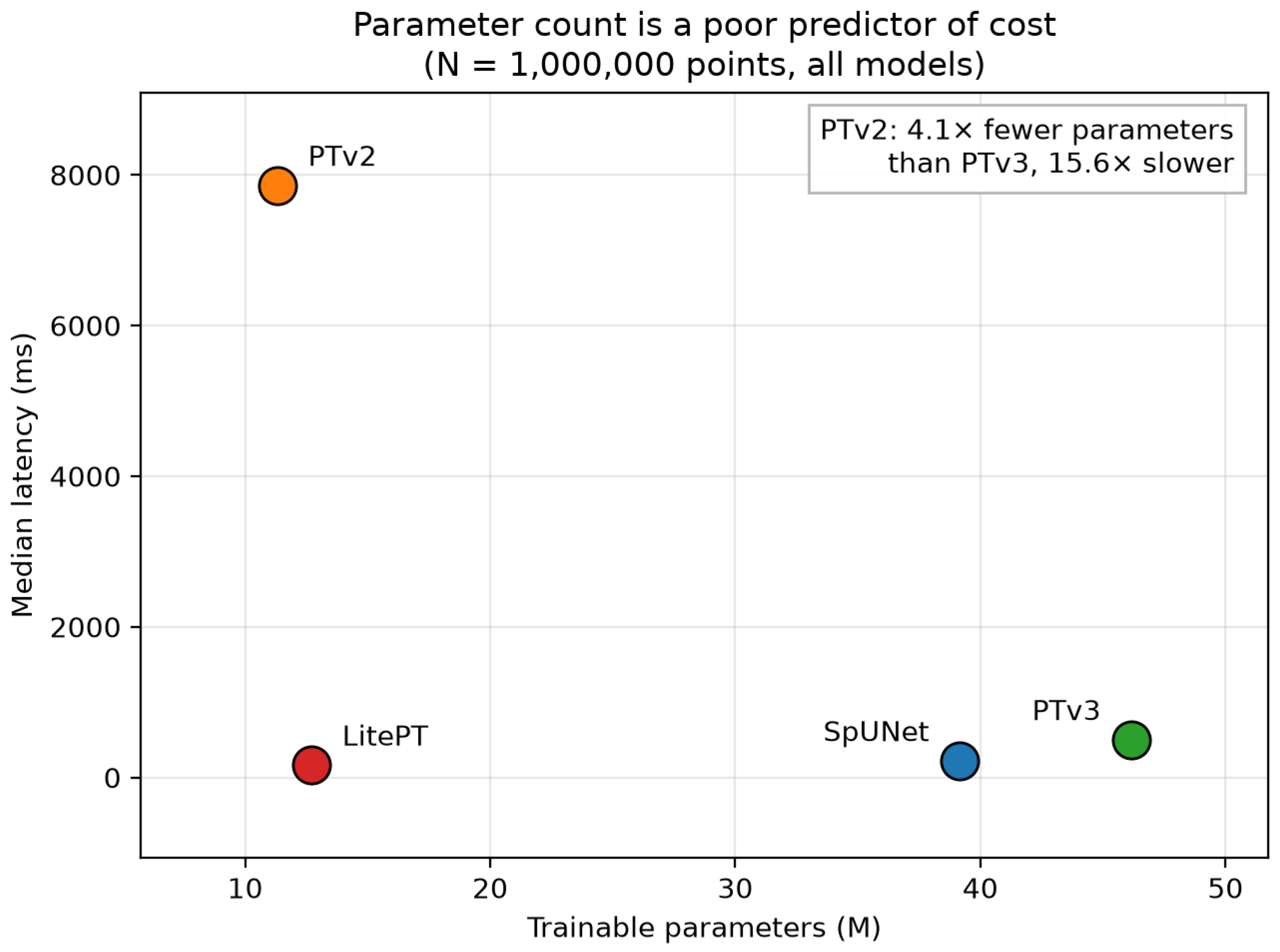
Table A1.
Controlled same-hardware cost profile of four point-cloud backbones at a common operating point of points on Paris-Lille-3D. All values are measured in this review on one 24 GB GPU at float32 on identical contiguous crops; each is the median over the two clouds of the dataset. Values marked † exclude custom CUDA kernels and are therefore lower bounds. Rows are ordered by latency. In this sample, parameter count neither predicts nor orders the deployment costs: the smallest model (PTv2) has the highest latency, memory, and energy, and the largest (PTv3) is lower than it on all three. Bold marks the best value in each column.
The mechanism is the one identified in Section 4. PTv2 spends its budget on grouped vector attention within neighborhoods that must be constructed explicitly, so its cost is set by the number of query–neighbor pairs rather than by its weight count; PTv3 replaces that construction with a serialization that is nearly free, and pays for a larger weight matrix instead. Parameters are a storage quantity. Latency, activation memory, and energy are governed by how many tokens the architecture forms and how it gathers them—which is why a parameter reduction cannot be reported as a speed claim.
The ratios between backbones are, moreover, not constants of the architectures. On Paris-Lille-3D, the latency ratio of PTv2 to PTv3 is at points, at , and at (, , and on SensatUrban, the last from a single tile), whereas the ratio of PTv3 to LitePT lies between and over all regimes that both complete, and their memory ratio is close to throughout. The published ratios ( and about ; Table 2) were obtained at the input sizes of driving and indoor benchmarks, on other hardware and with other settings. The comparison does not show those figures to be in error; it shows that a single headline ratio does not characterize a pair of architectures across input regimes.
Appendix A.3. Where the Backbones Stop
Table A2 and Figure A2 report how cost grows with tile size, and—more consequentially for deployment—at what tile size each backbone ceases to run at all. Within the regimes that complete, activation memory is close to linear in the number of input points for all four backbones, and latency is close to linear for LitePT, SpUNet, and PTv3, whose throughput is therefore roughly flat over one and a half orders of magnitude. PTv2 is the exception in slope as well as in level: its latency grows faster than linearly, by a factor of 27 for a tenfold increase in points on Paris-Lille-3D, so that it is slower than the hybrid at points and slower at .
Figure A2.
Scaling of median latency (left), peak activation memory (center), and throughput (right) with input size, for Paris-Lille-3D (top row) and SensatUrban (bottom row). Latency and memory axes are logarithmic. Within the regimes that complete, LitePT, SpUNet, and PTv3 grow close to linearly in the number of points, so their throughput is roughly flat and they separate by a near-constant factor; grouped vector attention (PTv2) is displaced upward by more than an order of magnitude, grows faster than linearly in latency, and meets the 24 GB device limit (dashed line) first. Series terminate where the backbone stops completing, and the causes of those terminations differ—see Table A2.
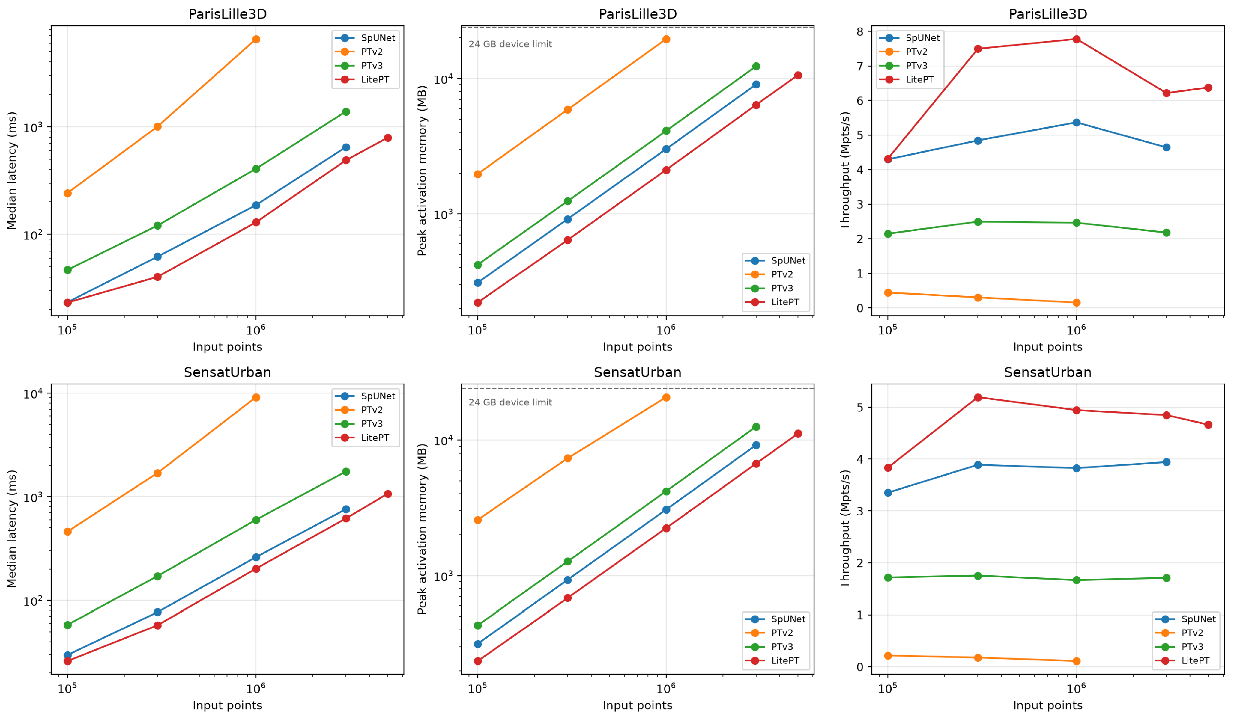
Table A2.
Scaling and failure behavior across input regimes, measured in this review. Upper panel: median forward latency (ms); lower panel: peak activation memory (MB); the italic rows in the table body are the panel headings. Each value is the median over the clouds of its dataset (two for Paris-Lille-3D, three for SensatUrban). oom denotes a clean exhaustion of the 24 GB device; err a fault inside a custom CUDA kernel that does not surface as a catchable out-of-memory condition—the two are distinguished deliberately, because they imply different remedies. A parenthesized value is a median over fewer clouds than the dataset contains, the remainder having failed. PL3D: Paris-Lille-3D; SU: SensatUrban.
The ceilings are where the practical argument of Section 4 is tested. On the 24 GB device used here, grouped vector attention (PTv2) exhausts memory at a three-million-point crop of Paris-Lille-3D and already at one million points on two of the three SensatUrban tiles; PTv3 completes three million and exhausts memory at five; LitePT reaches five million; and none of the four backbones—including the sparse-convolution baseline, whose memory growth is the most predictable of the four—completes a ten-million-point crop. Since a single birmingham_block_1 tile holds roughly 59 million points and the SensatUrban release comprises nearly three billion annotated points [37], tiling is unavoidable for these backbones on this hardware, and the quantity that distinguishes them operationally is how large a tile each admits, because tile size determines how much spatial context one inference sees and how many boundary artifacts must afterwards be reconciled.
The ceilings have different causes, and conflating them would itself be a P1 error. The PTv2 and PTv3 failures are clean out-of-memory conditions: the allocator reports exhaustion of the 24 GB device, and a larger device would move the ceiling. The failures of SpUNet at five million points and of LitePT, SpUNet, and PTv3 at ten million are not. SpUNet fails at five million inside an spconv size assertion on the product of point count and channel width, and the three backbones fail at ten million points with an illegal memory access raised asynchronously inside a custom CUDA kernel. The cause of that fault was not isolated. A diagnostic run excluded one candidate, overflow of the voxel-grid index: the grid volume of the ten-million-point crop is about cells, below the 32-bit limit, and coarsening the grid to 0.2 m did not remove the fault. The operational conclusion is bounded accordingly: none of the tested implementations processed a ten-million-point neighborhood in a single forward pass on this hardware, and for three of them, the limit is an implementation limit in the kernels of the current software stack rather than a memory limit, so a larger accelerator alone would not be expected to remove it. Whether the same holds for other implementations or software versions is not established here. The distinction matters because it determines whether the remedy is a larger accelerator or a corrected kernel, and it is invisible in any published figure that reports only the largest input a model was shown to handle.
Appendix A.4. What These Measurements Do and Do Not Establish
The absolute latencies are specific to one accelerator and would change on another; the claim is not that these are the costs of these architectures in general, but that they are their costs relative to one another when hardware, precision, input, head, and protocol are held fixed. That is the comparison the literature does not currently license, and it is obtainable at the cost of a single afternoon of compute—which is the argument of the standardized-protocol agenda item in Section 10.
The following limitations bound the reading, and no conclusion in the body of this review is intended to reach beyond them. Accuracy is out of scope, so the efficiency ordering here carries no implication about segmentation quality and must not be used as a proxy for it. The sample is four backbones, each in one configuration with untrained weights, on two datasets and five clouds: enough to provide a counterexample to parameter count as an efficiency proxy and to locate the tiling ceilings on this hardware, not enough to characterize the architecture space. One hardware class (a 24 GB laptop GPU), one precision (float32), and inference of a single crop at a time are measured; mixed precision, in which deployment commonly runs, batching, training cost, and edge or server accelerators are not. One voxel size (0.05 m) is used, although for the three voxel-based backbones, the voxel size controls the token count more directly than the crop size does, so a sweep over voxel sizes is the most informative extension of this benchmark. The laptop-class GPU may throttle under sustained load; the warm-up passes and the median over 20 timed passes limit the effect of transient clock changes, but clocks were not locked, so absolute latencies carry that additional uncertainty. Each configuration is measured once, on one crop per cloud, so variation between runs and between crops within a cloud is not characterized. The FLOP counts of three of the four backbones are lower bounds, for the reason given in Appendix A.1, and so bear less weight than the directly measured latency and memory; the energy figures are board-level estimates. Finally, the implementations are those of one codebase at one commit, with the attention-kernel difference between PTv3 and LitePT noted in Appendix A.1. Extending the measurements along each of these axes is the community task that Section 10 argues for.
References
- Khoramshahi, E.; Nezami, S.; Pellikka, P.; Honkavaara, E.; Chen, Y.; Habib, A. A Taxonomy of Sensors, Calibration and Computational Methods, and Applications of Mobile Mapping Systems: A Comprehensive Review. Remote Sens. 2025, 17, 1502. [Google Scholar] [CrossRef] [Scilit]
- Ravi, R.; Lin, Y.J.; Elbahnasawy, M.; Shamseldin, T.; Habib, A. Simultaneous System Calibration of a Multi-LiDAR Multicamera Mobile Mapping Platform. IEEE J. Sel. Top. Appl. Earth Obs. Remote Sens. 2018, 11, 1694–1714. [Google Scholar] [CrossRef] [Scilit]
- Elhashash, M.; Albanwan, H.; Qin, R. A Review of Mobile Mapping Systems: From Sensors to Applications. Sensors 2022, 22, 4262. [Google Scholar] [CrossRef] [Scilit]
- Wang, S.; Leroy, V.; Cabon, Y.; Chidlovskii, B.; Revaud, J. DUSt3R: Geometric 3D Vision Made Easy. In Proceedings of the IEEE/CVF Conference on Computer Vision and Pattern Recognition (CVPR), Seattle, WA, USA, 16–22 June 2024; IEEE: New York, NY, USA, 2024; pp. 20697–20709. [Google Scholar] [CrossRef] [Scilit]
- Leroy, V.; Cabon, Y.; Revaud, J. Grounding Image Matching in 3D with MASt3R. In Proceedings of the European Conference on Computer Vision (ECCV), Milan, Italy, 29 September–4 October 2024; pp. 71–91. [Google Scholar] [CrossRef] [Scilit]
- Wang, J.; Chen, M.; Karaev, N.; Vedaldi, A.; Rupprecht, C.; Novotny, D. VGGT: Visual Geometry Grounded Transformer. In Proceedings of the IEEE/CVF Conference on Computer Vision and Pattern Recognition (CVPR), Nashville, TN, USA, 10–17 June 2025; IEEE: New York, NY, USA, 2025; pp. 5294–5306. [Google Scholar] [CrossRef] [Scilit]
- Strasdat, H.; Montiel, J.M.M.; Davison, A.J. Scale Drift-Aware Large Scale Monocular SLAM. In Proceedings of the Robotics: Science and Systems (RSS), Zaragoza, Spain, 27–30 June 2010. [Google Scholar] [CrossRef] [Scilit]
- Campos, C.; Elvira, R.; Gómez Rodríguez, J.J.; Montiel, J.M.M.; Tardós, J.D. ORB-SLAM3: An Accurate Open-Source Library for Visual, Visual–Inertial, and Multimap SLAM. IEEE Trans. Robot. 2021, 37, 1874–1890. [Google Scholar] [CrossRef] [Scilit]
- Shan, T.; Englot, B.; Meyers, D.; Wang, W.; Ratti, C.; Rus, D. LIO-SAM: Tightly-Coupled Lidar Inertial Odometry via Smoothing and Mapping. In Proceedings of the IEEE/RSJ International Conference on Intelligent Robots and Systems (IROS), Las Vegas, NV, USA, 25–29 October 2020; IEEE: New York, NY, USA, 2020; pp. 5135–5142. [Google Scholar] [CrossRef] [Scilit]
- Wang, W.; Li, H.; Yu, H.; Xie, Q.; Dong, J.; Sun, X.; Liu, H.; Sun, C.; Li, B.; Zheng, F. SLAM Algorithm for Mobile Robots Based on Improved LVI-SAM in Complex Environments. Sensors 2024, 24, 7214. [Google Scholar] [CrossRef] [Scilit]
- Xu, W.; Cai, Y.; He, D.; Lin, J.; Zhang, F. FAST-LIO2: Fast Direct LiDAR-Inertial Odometry. IEEE Trans. Robot. 2022, 38, 2053–2073. [Google Scholar] [CrossRef] [Scilit]
- Vaswani, A.; Shazeer, N.; Parmar, N.; Uszkoreit, J.; Jones, L.; Gomez, A.N.; Kaiser, Ł.; Polosukhin, I. Attention Is All You Need. In Proceedings of the Advances in Neural Information Processing Systems (NeurIPS), Long Beach, CA, USA, 4–9 December 2017; Volume 30. [Google Scholar]
- Zhao, H.; Jiang, L.; Jia, J.; Torr, P.; Koltun, V. Point Transformer. In Proceedings of the IEEE/CVF International Conference on Computer Vision (ICCV), Montreal, QC, Canada, 10–17 October 2021; IEEE: New York, NY, USA, 2021; pp. 16239–16248. [Google Scholar] [CrossRef] [Scilit]
- Wu, X.; Lao, Y.; Jiang, L.; Liu, X.; Zhao, H. Point Transformer V2: Grouped Vector Attention and Partition-Based Pooling. In Proceedings of the Advances in Neural Information Processing Systems (NeurIPS), New Orleans, LA, USA, 28 November–9 December 2022; pp. 33330–33342. [Google Scholar] [CrossRef] [Scilit]
- Wu, X.; Jiang, L.; Wang, P.S.; Liu, Z.; Liu, X.; Qiao, Y.; Ouyang, W.; He, T.; Zhao, H. Point Transformer V3: Simpler, Faster, Stronger. In Proceedings of the IEEE/CVF Conference on Computer Vision and Pattern Recognition (CVPR), Seattle, WA, USA, 16–22 June 2024; IEEE: New York, NY, USA, 2024; pp. 4840–4851. [Google Scholar] [CrossRef] [Scilit]
- Qi, C.R.; Su, H.; Mo, K.; Guibas, L.J. PointNet: Deep Learning on Point Sets for 3D Classification and Segmentation. In Proceedings of the IEEE/CVF Conference on Computer Vision and Pattern Recognition (CVPR), Honolulu, HI, USA, 21–26 July 2017; IEEE: New York, NY, USA, 2017; pp. 77–85. [Google Scholar] [CrossRef] [Scilit]
- Qi, C.R.; Yi, L.; Su, H.; Guibas, L.J. PointNet++: Deep Hierarchical Feature Learning on Point Sets in a Metric Space. In Proceedings of the Advances in Neural Information Processing Systems (NeurIPS), Long Beach, CA, USA, 4–9 December 2017. [Google Scholar]
- Thomas, H.; Qi, C.R.; Deschaud, J.E.; Marcotegui, B.; Goulette, F.; Guibas, L.J. KPConv: Flexible and Deformable Convolution for Point Clouds. In Proceedings of the IEEE/CVF International Conference on Computer Vision (ICCV), Seoul, Republic of Korea, 27 October–2 November 2019; IEEE: New York, NY, USA, 2019; pp. 6410–6419. [Google Scholar] [CrossRef] [Scilit]
- Choy, C.; Gwak, J.; Savarese, S. 4D Spatio-Temporal ConvNets: Minkowski Convolutional Neural Networks. In Proceedings of the IEEE/CVF Conference on Computer Vision and Pattern Recognition (CVPR), Long Beach, CA, USA, 15–20 June 2019; IEEE: New York, NY, USA, 2019; pp. 3070–3079. [Google Scholar] [CrossRef] [Scilit]
- Wang, X.; Zhang, Y.; Shao, R.; Chen, S.; Li, H.; Chen, X. SAT-Former: An Efficient 3-D Transformer with Semantic Aggregated Point Tokenizer for Point Cloud Semantic Segmentation in Urban Scenes. IEEE J. Sel. Top. Appl. Earth Obs. Remote Sens. 2025, 18, 28326–28342. [Google Scholar] [CrossRef] [Scilit]
- Yue, Y.; Robert, D.; Wang, J.; Hong, S.; Wegner, J.D.; Rupprecht, C.; Schindler, K. LitePT: Lighter Yet Stronger Point Transformer. In Proceedings of the IEEE/CVF Conference on Computer Vision and Pattern Recognition (CVPR), Denver, CO, USA, 3–7 June 2026; IEEE: New York, NY, USA, 2026; pp. 24173–24184. [Google Scholar]
- Tewari, A.; Thies, J.; Mildenhall, B.; Srinivasan, P.; Tretschk, E.; Yifan, W.; Lassner, C.; Sitzmann, V.; Martin-Brualla, R.; Lombardi, S.; et al. Advances in Neural Rendering. Comput. Graph. Forum 2022, 41, 703–735. [Google Scholar] [CrossRef] [Scilit]
- Xie, Y.; Takikawa, T.; Saito, S.; Litany, O.; Yan, S.; Khan, N.; Tombari, F.; Tompkin, J.; Sitzmann, V.; Sridhar, S. Neural Fields in Visual Computing and Beyond. Comput. Graph. Forum 2022, 41, 641–676. [Google Scholar] [CrossRef] [Scilit]
- Barron, J.T.; Mildenhall, B.; Verbin, D.; Srinivasan, P.P.; Hedman, P. Mip-NeRF 360: Unbounded Anti-Aliased Neural Radiance Fields. In Proceedings of the IEEE/CVF Conference on Computer Vision and Pattern Recognition (CVPR), New Orleans, LA, USA, 18–24 June 2022; IEEE: New York, NY, USA, 2022; pp. 5460–5469. [Google Scholar] [CrossRef] [Scilit]
- Mildenhall, B.; Srinivasan, P.P.; Tancik, M.; Barron, J.T.; Ramamoorthi, R.; Ng, R. NeRF: Representing Scenes as Neural Radiance Fields for View Synthesis. In Proceedings of the European Conference on Computer Vision (ECCV), Glasgow, UK, 23–28 August 2020; pp. 405–421. [Google Scholar] [CrossRef] [Scilit]
- Kerbl, B.; Kopanas, G.; Leimkühler, T.; Drettakis, G. 3D Gaussian Splatting for Real-Time Radiance Field Rendering. ACM Trans. Graph. 2023, 42, 139. [Google Scholar] [CrossRef] [Scilit]
- Chen, G.; Wang, W. A Survey on 3D Gaussian Splatting. ACM Comput. Surv. 2026, 58, 313. [Google Scholar] [CrossRef] [Scilit]
- Jakubik, J.; Roy, S.; Phillips, C.E.; Fraccaro, P.; Godwin, D.; Zadrozny, B.; Szwarcman, D.; Gomes, C.; Nyirjesy, G.; Edwards, B.; et al. Foundation Models for Generalist Geospatial Artificial Intelligence. arXiv 2023, arXiv:2310.18660. [Google Scholar] [CrossRef] [Scilit]
- Mendieta, M.; Han, B.; Shi, X.; Zhu, Y.; Chen, C.; Li, M. Towards Geospatial Foundation Models via Continual Pretraining. In Proceedings of the IEEE/CVF International Conference on Computer Vision (ICCV), Paris, France, 1–6 October 2023; IEEE: New York, NY, USA, 2023; pp. 16760–16770. [Google Scholar] [CrossRef] [Scilit]
- Reed, C.J.; Gupta, R.; Li, S.; Brockman, S.; Funk, C.; Clipp, B.; Keutzer, K.; Candido, S.; Uyttendaele, M.; Darrell, T. Scale-MAE: A Scale-Aware Masked Autoencoder for Multiscale Geospatial Representation Learning. In Proceedings of the IEEE/CVF International Conference on Computer Vision (ICCV), Paris, France, 1–6 October 2023; IEEE: New York, NY, USA, 2023; pp. 4065–4076. [Google Scholar] [CrossRef] [Scilit]
- Bell, A.; Aides, A.; Helmy, A.; Muslim, A.; Barzilai, A.; Slobodkin, A.; Jaber, B.; Schottlander, D.; Leifman, G.; Paul, J.; et al. Earth AI: Unlocking Geospatial Insights with Foundation Models and Cross-Modal Reasoning. arXiv 2025, arXiv:2510.18318. [Google Scholar] [CrossRef] [Scilit]
- Li, Z.; Ning, H. Autonomous GIS: The Next-Generation AI-Powered GIS. Int. J. Digit. Earth 2023, 16, 4668–4686. [Google Scholar] [CrossRef] [Scilit]
- Kölle, M.; Laupheimer, D.; Schmohl, S.; Haala, N.; Rottensteiner, F.; Wegner, J.D.; Ledoux, H. The Hessigheim 3D (H3D) benchmark on semantic segmentation of high-resolution 3D point clouds and textured meshes from UAV LiDAR and Multi-View-Stereo. ISPRS Open J. Photogramm. Remote Sens. 2021, 1, 100001. [Google Scholar] [CrossRef] [Scilit]
- Lehtola, V.V.; Koeva, M.; Oude Elberink, S.; Raposo, P.; Virtanen, J.P.; Vahdatikhaki, F.; Borsci, S. Digital twin of a city: Review of technology serving city needs. Int. J. Appl. Earth Obs. Geoinf. 2022, 114, 102915. [Google Scholar] [CrossRef] [Scilit]
- Roynard, X.; Deschaud, J.E.; Goulette, F. Paris-Lille-3D: A Large and High-Quality Ground-Truth Urban Point Cloud Dataset for Automatic Segmentation and Classification. Int. J. Robot. Res. 2018, 37, 545–557. [Google Scholar] [CrossRef] [Scilit]
- Varney, N.; Asari, V.K.; Graehling, Q. DALES: A Large-Scale Aerial LiDAR Data Set for Semantic Segmentation. In Proceedings of the IEEE/CVF Conference on Computer Vision and Pattern Recognition Workshops (CVPRW), Seattle, WA, USA, 14–19 June 2020; IEEE: New York, NY, USA, 2020; pp. 717–726. [Google Scholar] [CrossRef] [Scilit]
- Hu, Q.; Yang, B.; Khalid, S.; Xiao, W.; Trigoni, N.; Markham, A. Towards Semantic Segmentation of Urban-Scale 3D Point Clouds: A Dataset, Benchmarks and Challenges. In Proceedings of the IEEE/CVF Conference on Computer Vision and Pattern Recognition (CVPR), Nashville, TN, USA, 20–25 June 2021; IEEE: New York, NY, USA, 2021; pp. 4975–4985. [Google Scholar] [CrossRef] [Scilit]
- Dwork, C. Differential Privacy. In Proceedings of the International Colloquium on Automata, Languages and Programming (ICALP), Venice, Italy, 10–14 July 2006; pp. 1–12. [Google Scholar] [CrossRef] [Scilit]
- Guo, Y.; Wang, H.; Hu, Q.; Liu, H.; Liu, L.; Bennamoun, M. Deep Learning for 3D Point Clouds: A Survey. IEEE Trans. Pattern Anal. Mach. Intell. 2021, 43, 4338–4364. [Google Scholar] [CrossRef] [Scilit]
- Bello, S.A.; Yu, S.; Wang, C.; Adam, J.M.; Li, J. Review: Deep Learning on 3D Point Clouds. Remote Sens. 2020, 12, 1729. [Google Scholar] [CrossRef] [Scilit]
- Xie, Y.; Tian, J.; Zhu, X.X. Linking Points With Labels in 3D: A Review of Point Cloud Semantic Segmentation. IEEE Geosci. Remote Sens. Mag. 2020, 8, 38–59. [Google Scholar] [CrossRef] [Scilit]
- Fei, B.; Xu, J.; Zhang, R.; Zhou, Q.; Yang, W.; He, Y. 3D Gaussian Splatting as New Era: A Survey. IEEE Trans. Vis. Comput. Graph. 2025, 31, 4429–4449. [Google Scholar] [CrossRef] [Scilit]
- Grant, M.J.; Booth, A. A typology of reviews: An analysis of 14 review types and associated methodologies. Health Inf. Libr. J. 2009, 26, 91–108. [Google Scholar] [CrossRef] [Scilit]
- Page, M.J.; McKenzie, J.E.; Bossuyt, P.M.; Boutron, I.; Hoffmann, T.C.; Mulrow, C.D.; Shamseer, L.; Tetzlaff, J.M.; Akl, E.A.; Brennan, S.E.; et al. The PRISMA 2020 statement: An updated guideline for reporting systematic reviews. BMJ 2021, 372, n71. [Google Scholar] [CrossRef] [Scilit]
- Wohlin, C. Guidelines for snowballing in systematic literature studies and a replication in software engineering. In Proceedings of the International Conference on Evaluation and Assessment in Software Engineering (EASE), London, UK, 13–14 May 2014; pp. 1–10. [Google Scholar] [CrossRef] [Scilit]
- Deng, Y.; Ai, H.; Deng, Z.; Gao, W.; Shang, J. An Overview of Indoor Positioning and Mapping Technology Standards. Standards 2022, 2, 157–183. [Google Scholar] [CrossRef] [Scilit]
- Liang, X.; Hyyppä, J.; Kaartinen, H.; Lehtomäki, M.; Pyörälä, J.; Pfeifer, N.; Holopainen, M.; Brolly, G.; Francesco, P.; Hackenberg, J.; et al. International benchmarking of terrestrial laser scanning approaches for forest inventories. ISPRS J. Photogramm. Remote Sens. 2018, 144, 137–179. [Google Scholar] [CrossRef] [Scilit]
- Calders, K.; Adams, J.; Armston, J.; Bartholomeus, H.; Bauwens, S.; Bentley, L.P.; Chave, J.; Danson, F.M.; Demol, M.; Disney, M.; et al. Terrestrial laser scanning in forest ecology: Expanding the horizon. Remote Sens. Environ. 2020, 251, 112102. [Google Scholar] [CrossRef] [Scilit]
- Skaloud, J.; Lichti, D. Rigorous approach to bore-sight self-calibration in airborne laser scanning. ISPRS J. Photogramm. Remote Sens. 2006, 61, 47–59, Erratum in ISPRS J. Photogramm. Remote Sens. 2007, 61, 414–415. https://doi.org/10.1016/j.isprsjprs.2006.11.001. [Google Scholar] [CrossRef] [Scilit]
- Glennie, C. Rigorous 3D error analysis of kinematic scanning LIDAR systems. J. Appl. Geod. 2007, 1, 147–157. [Google Scholar] [CrossRef] [Scilit]
- Altamimi, Z.; Rebischung, P.; Collilieux, X.; Métivier, L.; Chanard, K. ITRF2020: An augmented reference frame refining the modeling of nonlinear station motions. J. Geod. 2023, 97, 47. [Google Scholar] [CrossRef] [Scilit]
- Abdullah, Q.; Munjy, R.; Nimetz, J.; Zoltek, M.; Lee, C. ASPRS Positional Accuracy Standards for Digital Geospatial Data, 2nd ed.; American Society for Photogrammetry and Remote Sensing: Baton Rouge, LA, USA, 2024. [Google Scholar] [CrossRef] [Scilit]
- Kaartinen, H.; Hyyppä, J.; Kukko, A.; Jaakkola, A.; Hyyppä, H. Benchmarking the Performance of Mobile Laser Scanning Systems Using a Permanent Test Field. Sensors 2012, 12, 12814–12835. [Google Scholar] [CrossRef] [Scilit]
- Baarda, W. A Testing Procedure for Use in Geodetic Networks. Volume 2: Publications on Geodesy, New Series; Netherlands Geodetic Commission: Delft, The Netherlands, 1968. [Google Scholar]
- Förstner, W.; Wrobel, B.P. Photogrammetric Computer Vision: Statistics, Geometry, Orientation and Reconstruction. Volume 11: Geometry and Computing; Springer: Cham, Switzerland, 2016. [Google Scholar] [CrossRef] [Scilit]
- Maggio, D.; Carlone, L. VGGT-SLAM 2.0: Real-Time Dense Feed-Forward Scene Reconstruction. In Proceedings of the Robotics: Science and Systems (RSS), Sydney, Australia, 13–17 July 2026. [Google Scholar] [CrossRef] [Scilit]
- Maggio, D.; Lim, H.; Carlone, L. VGGT-SLAM: Dense RGB SLAM Optimized on the SL(4) Manifold. In Proceedings of the Advances in Neural Information Processing Systems (NeurIPS), San Diego, CA, USA, 30 November–7 December 2025; pp. 143976–144004. [Google Scholar] [CrossRef] [Scilit]
- Teed, Z.; Deng, J. DROID-SLAM: Deep Visual SLAM for Monocular, Stereo, and RGB-D Cameras. In Proceedings of the Advances in Neural Information Processing Systems (NeurIPS), Virtual, 6–14 December 2021; Volume 34, pp. 16558–16569. [Google Scholar]
- Murai, R.; Dexheimer, E.; Davison, A.J. MASt3R-SLAM: Real-Time Dense SLAM with 3D Reconstruction Priors. In Proceedings of the IEEE/CVF Conference on Computer Vision and Pattern Recognition (CVPR), Nashville, TN, USA, 10–17 June 2025; IEEE: New York, NY, USA, 2025; pp. 16695–16705. [Google Scholar] [CrossRef] [Scilit]
- Zhu, Z.; Peng, S.; Larsson, V.; Xu, W.; Bao, H.; Cui, Z.; Oswald, M.R.; Pollefeys, M. NICE-SLAM: Neural Implicit Scalable Encoding for SLAM. In Proceedings of the IEEE/CVF Conference on Computer Vision and Pattern Recognition (CVPR), New Orleans, LA, USA, 18–24 June 2022; IEEE: New York, NY, USA, 2022; pp. 12776–12786. [Google Scholar] [CrossRef] [Scilit]
- Wang, H.; Wang, J.; Agapito, L. Co-SLAM: Joint Coordinate and Sparse Parametric Encodings for Neural Real-Time SLAM. In Proceedings of the IEEE/CVF Conference on Computer Vision and Pattern Recognition (CVPR), Vancouver, BC, Canada, 17–24 June 2023; IEEE: New York, NY, USA, 2023; pp. 13293–13302. [Google Scholar] [CrossRef] [Scilit]
- Hu, J.; Mao, M.; Bao, H.; Zhang, G.; Cui, Z. CP-SLAM: Collaborative Neural Point-Based SLAM System. In Proceedings of the Advances in Neural Information Processing Systems (NeurIPS), New Orleans, LA, USA, 10–16 December 2023; pp. 39429–39442. [Google Scholar] [CrossRef] [Scilit]
- Kukko, A.; Kaijaluoto, R.; Kaartinen, H.; Lehtola, V.V.; Jaakkola, A.; Hyyppä, J. Graph SLAM correction for single scanner MLS forest data under boreal forest canopy. ISPRS J. Photogramm. Remote Sens. 2017, 132, 199–209. [Google Scholar] [CrossRef] [Scilit]
- Qian, C.; Liu, H.; Tang, J.; Chen, Y.; Kaartinen, H.; Kukko, A.; Zhu, L.; Liang, X.; Chen, L.; Hyyppä, J. An Integrated GNSS/INS/LiDAR-SLAM Positioning Method for Highly Accurate Forest Stem Mapping. Remote Sens. 2017, 9, 3. [Google Scholar] [CrossRef] [Scilit]
- Pierzchała, M.; Giguère, P.; Astrup, R. Mapping forests using an unmanned ground vehicle with 3D LiDAR and graph-SLAM. Comput. Electron. Agric. 2018, 145, 217–225. [Google Scholar] [CrossRef] [Scilit]
- Bauwens, S.; Bartholomeus, H.; Calders, K.; Lejeune, P. Forest Inventory with Terrestrial LiDAR: A Comparison of Static and Hand-Held Mobile Laser Scanning. Forests 2016, 7, 127. [Google Scholar] [CrossRef] [Scilit]
- Cabo, C.; Del Pozo, S.; Rodríguez-Gonzálvez, P.; Ordóñez, C.; González-Aguilera, D. Comparing Terrestrial Laser Scanning (TLS) and Wearable Laser Scanning (WLS) for Individual Tree Modeling at Plot Level. Remote Sens. 2018, 10, 540. [Google Scholar] [CrossRef] [Scilit]
- Hyyppä, E.; Hyyppä, J.; Hakala, T.; Kukko, A.; Wulder, M.A.; White, J.C.; Pyörälä, J.; Yu, X.; Wang, Y.; Virtanen, J.P.; et al. Under-canopy UAV laser scanning for accurate forest field measurements. ISPRS J. Photogramm. Remote Sens. 2020, 164, 41–60. [Google Scholar] [CrossRef] [Scilit]
- Muhojoki, J.; Tavi, D.; Hyyppä, E.; Lehtomäki, M.; Faitli, T.; Kaartinen, H.; Kukko, A.; Hakala, T.; Hyyppä, J. Benchmarking Under- and Above-Canopy Laser Scanning Solutions for Deriving Stem Curve and Volume in Easy and Difficult Boreal Forest Conditions. Remote Sens. 2024, 16, 1721. [Google Scholar] [CrossRef] [Scilit]
- Proudman, A.; Ramezani, M.; Digumarti, S.T.; Chebrolu, N.; Fallon, M. Towards real-time forest inventory using handheld LiDAR. Robot. Auton. Syst. 2022, 157, 104240. [Google Scholar] [CrossRef] [Scilit]
- Vora, S.; Lang, A.H.; Helou, B.; Beijbom, O. PointPainting: Sequential Fusion for 3D Object Detection. In Proceedings of the IEEE/CVF Conference on Computer Vision and Pattern Recognition (CVPR), Seattle, WA, USA, 13–19 June 2020; IEEE: New York, NY, USA, 2020; pp. 4603–4611. [Google Scholar] [CrossRef] [Scilit]
- Bai, X.; Hu, Z.; Zhu, X.; Huang, Q.; Chen, Y.; Fu, H.; Tai, C.L. TransFusion: Robust LiDAR-Camera Fusion for 3D Object Detection with Transformers. In Proceedings of the IEEE/CVF Conference on Computer Vision and Pattern Recognition (CVPR), New Orleans, LA, USA, 18–24 June 2022; IEEE: New York, NY, USA, 2022; pp. 1080–1089. [Google Scholar] [CrossRef] [Scilit]
- Liu, Z.; Tang, H.; Amini, A.; Yang, X.; Mao, H.; Rus, D.; Han, S. BEVFusion: Multi-Task Multi-Sensor Fusion with Unified Bird’s-Eye View Representation. In Proceedings of the IEEE International Conference on Robotics and Automation (ICRA), London, UK, 29 May–2 June 2023; IEEE: New York, NY, USA, 2023; pp. 2774–2781. [Google Scholar] [CrossRef] [Scilit]
- Chen, S.; Yan, Q.; Qu, Y.; Gao, W.; Yang, J.; Deng, F. Ortho-NeRF: Generating a True Digital Orthophoto Map Using the Neural Radiance Field from Unmanned Aerial Vehicle Images. Geo-Spat. Inf. Sci. 2025, 28, 741–760. [Google Scholar] [CrossRef] [Scilit]
- Zhang, Y.; Chen, G.; Chen, J.; Cui, S. Aerial Lifting: Neural Urban Semantic and Building Instance Lifting from Aerial Imagery. In Proceedings of the IEEE/CVF Conference on Computer Vision and Pattern Recognition (CVPR), Seattle, WA, USA, 16–22 June 2024; IEEE: New York, NY, USA, 2024; pp. 21092–21103. [Google Scholar] [CrossRef] [Scilit]
- Remondino, F.; Karami, A.; Yan, Z.; Mazzacca, G.; Rigon, S.; Qin, R. A Critical Analysis of NeRF-Based 3D Reconstruction. Remote Sens. 2023, 15, 3585. [Google Scholar] [CrossRef] [Scilit]
- Hillemann, M.; Langendörfer, R.; Landgraf, S.; Ulrich, M. Uncertainty Quality of VGGT: An Analysis on the DTU Benchmark Dataset. ISPRS Ann. Photogramm. Remote Sens. Spat. Inf. Sci. 2026, XI-2-2026, 665–672. [Google Scholar] [CrossRef] [Scilit]
- Qiu, Y.; Chen, Y.; Zhang, Z.; Wang, W.; Scherer, S. MAC-VO: Metrics-Aware Covariance for Learning-Based Stereo Visual Odometry. In Proceedings of the IEEE International Conference on Robotics and Automation (ICRA), Atlanta, GA, USA, 19–23 May 2025; IEEE: New York, NY, USA, 2025; pp. 3803–3814. [Google Scholar] [CrossRef] [Scilit]
- Graham, B.; Engelcke, M.; van der Maaten, L. 3D Semantic Segmentation with Submanifold Sparse Convolutional Networks. In Proceedings of the IEEE/CVF Conference on Computer Vision and Pattern Recognition (CVPR), Salt Lake City, UT, USA, 18–23 June 2018; IEEE: New York, NY, USA, 2018; pp. 9224–9232. [Google Scholar] [CrossRef] [Scilit]
- Hu, Q.; Yang, B.; Xie, L.; Rosa, S.; Guo, Y.; Wang, Z.; Trigoni, N.; Markham, A. RandLA-Net: Efficient Semantic Segmentation of Large-Scale Point Clouds. In Proceedings of the IEEE/CVF Conference on Computer Vision and Pattern Recognition (CVPR), Seattle, WA, USA, 13–19 June 2020; IEEE: New York, NY, USA, 2020; pp. 11105–11114. [Google Scholar] [CrossRef] [Scilit]
- Lai, X.; Liu, J.; Jiang, L.; Wang, L.; Zhao, H.; Liu, S.; Qi, X.; Jia, J. Stratified Transformer for 3D Point Cloud Segmentation. In Proceedings of the IEEE/CVF Conference on Computer Vision and Pattern Recognition (CVPR), New Orleans, LA, USA, 18–24 June 2022; IEEE: New York, NY, USA, 2022; pp. 8490–8499. [Google Scholar] [CrossRef] [Scilit]
- Wang, P.S. OctFormer: Octree-Based Transformers for 3D Point Clouds. ACM Trans. Graph. (SIGGRAPH) 2023, 42, 155. [Google Scholar] [CrossRef] [Scilit]
- Liu, S.; Fu, K.; Wang, M.; Song, Z. Group-in-Group Relation-Based Transformer for 3D Point Cloud Learning. Remote Sens. 2022, 14, 1563. [Google Scholar] [CrossRef] [Scilit]
- Monji-Azad, S.; Kinz, M.; Kothari, S.; Khanna, R.; Mihan, A.C.; Maennel, D.; Scherl, C.; Hesser, J. DefTransNet: A Transformer-Based Method for Non-Rigid Point Cloud Registration in the Simulation of Soft Tissue Deformation. Meas. Sci. Technol. 2025, 36, 076006. [Google Scholar] [CrossRef] [Scilit]
- Tran, T.A.; Nguyen, D.M.H.; Tran, H.C.; Barz, M.; Doan, K.D.; Wattenhofer, R.; Vien, N.A.; Niepert, M.; Sonntag, D.; Swoboda, P. How Many Tokens Do 3D Point Cloud Transformer Architectures Really Need? In Proceedings of the Advances in Neural Information Processing Systems (NeurIPS), San Diego, CA, USA, 30 November–7 December 2025; pp. 15106–15138. [Google Scholar] [CrossRef] [Scilit]
- Lu, D.; Xie, Q.; Gao, K.; Xu, L.; Li, J. 3DCTN: 3D Convolution-Transformer Network for Point Cloud Classification. IEEE Trans. Intell. Transp. Syst. 2022, 23, 24854–24865. [Google Scholar] [CrossRef] [Scilit]
- Wu, X.; DeTone, D.; Frost, D.; Shen, T.; Xie, C.; Yang, N.; Engel, J.; Newcombe, R.; Zhao, H.; Straub, J. Sonata: Self-Supervised Learning of Reliable Point Representations. In Proceedings of the IEEE/CVF Conference on Computer Vision and Pattern Recognition (CVPR), Nashville, TN, USA, 10–17 June 2025; IEEE: New York, NY, USA, 2025; pp. 22193–22204. [Google Scholar] [CrossRef] [Scilit]
- Hackel, T.; Savinov, N.; Ladicky, L.; Wegner, J.D.; Schindler, K.; Pollefeys, M. Semantic3D.net: A New Large-Scale Point Cloud Classification Benchmark. ISPRS Ann. Photogramm. Remote Sens. Spat. Inf. Sci. 2017, IV-1/W1, 91–98. [Google Scholar] [CrossRef] [Scilit]
- Tan, W.; Qin, N.; Ma, L.; Li, Y.; Du, J.; Cai, G.; Yang, K.; Li, J. Toronto-3D: A Large-Scale Mobile LiDAR Dataset for Semantic Segmentation of Urban Roadways. In Proceedings of the IEEE/CVF Conference on Computer Vision and Pattern Recognition Workshops (CVPRW), Seattle, WA, USA, 14–19 June 2020; IEEE: New York, NY, USA, 2020; pp. 797–806. [Google Scholar] [CrossRef] [Scilit]
- Behley, J.; Garbade, M.; Milioto, A.; Quenzel, J.; Behnke, S.; Stachniss, C.; Gall, J. SemanticKITTI: A Dataset for Semantic Scene Understanding of LiDAR Sequences. In Proceedings of the IEEE/CVF International Conference on Computer Vision (ICCV), Seoul, Republic of Korea, 27 October–2 November 2019; IEEE: New York, NY, USA, 2019; pp. 9296–9306. [Google Scholar] [CrossRef] [Scilit]
- Caesar, H.; Bankiti, V.; Lang, A.H.; Vora, S.; Liong, V.E.; Xu, Q.; Krishnan, A.; Pan, Y.; Baldan, G.; Beijbom, O. nuScenes: A Multimodal Dataset for Autonomous Driving. In Proceedings of the IEEE/CVF Conference on Computer Vision and Pattern Recognition (CVPR), Seattle, WA, USA, 13–19 June 2020; IEEE: New York, NY, USA, 2020; pp. 11618–11628. [Google Scholar] [CrossRef] [Scilit]
- Sun, P.; Kretzschmar, H.; Dotiwalla, X.; Chouard, A.; Patnaik, V.; Tsui, P.; Guo, J.; Zhou, Y.; Chai, Y.; Caine, B.; et al. Scalability in Perception for Autonomous Driving: Waymo Open Dataset. In Proceedings of the IEEE/CVF Conference on Computer Vision and Pattern Recognition (CVPR), Seattle, WA, USA, 13–19 June 2020; IEEE: New York, NY, USA, 2020; pp. 2443–2451. [Google Scholar] [CrossRef] [Scilit]
- Liao, Y.; Xie, J.; Geiger, A. KITTI-360: A Novel Dataset and Benchmarks for Urban Scene Understanding in 2D and 3D. IEEE Trans. Pattern Anal. Mach. Intell. 2023, 45, 3292–3310. [Google Scholar] [CrossRef] [Scilit]
- Armeni, I.; Sener, O.; Zamir, A.R.; Jiang, H.; Brilakis, I.; Fischer, M.; Savarese, S. 3D Semantic Parsing of Large-Scale Indoor Spaces. In Proceedings of the IEEE/CVF Conference on Computer Vision and Pattern Recognition (CVPR), Las Vegas, NV, USA, 27–30 June 2016; IEEE: New York, NY, USA, 2016; pp. 1534–1543. [Google Scholar] [CrossRef] [Scilit]
- Dai, A.; Chang, A.X.; Savva, M.; Halber, M.; Funkhouser, T.; Nießner, M. ScanNet: Richly-Annotated 3D Reconstructions of Indoor Scenes. In Proceedings of the IEEE/CVF Conference on Computer Vision and Pattern Recognition (CVPR), Honolulu, HI, USA, 21–26 July 2017; IEEE: New York, NY, USA, 2017; pp. 2432–2443. [Google Scholar] [CrossRef] [Scilit]
- Rottensteiner, F.; Sohn, G.; Jung, J.; Gerke, M.; Baillard, C.; Benitez, S.; Breitkopf, U. The ISPRS Benchmark on Urban Object Classification and 3D Building Reconstruction. ISPRS Ann. Photogramm. Remote Sens. Spat. Inf. Sci. 2012, I–3, 293–298. [Google Scholar] [CrossRef] [Scilit]
- Chen, M.; Hu, Q.; Yu, Z.; Thomas, H.; Feng, A.; Hou, Y.; McCullough, K.; Ren, F.; Soibelman, L. STPLS3D: A Large-Scale Synthetic and Real Aerial Photogrammetry 3D Point Cloud Dataset. In Proceedings of the British Machine Vision Conference (BMVC), London, UK, 21–24 November 2022. [Google Scholar]
- Gaydon, C.; Daab, M.; Roche, F. FRACTAL: An ultra-large-scale aerial lidar dataset for 3D semantic segmentation of diverse landscapes. arXiv 2024, arXiv:2405.04634. [Google Scholar] [CrossRef] [Scilit]
- Puliti, S.; Pearse, G.; Surový, P.; Wallace, L.; Hollaus, M.; Wielgosz, M.; Astrup, R. FOR-instance: A UAV Laser Scanning Benchmark Dataset for Semantic and Instance Segmentation of Individual Trees. arXiv 2023, arXiv:2309.01279. [Google Scholar] [CrossRef] [Scilit]
- Wielgosz, M.; Puliti, S.; Xiang, B.; Schindler, K.; Astrup, R. SegmentAnyTree: A sensor and platform agnostic deep learning model for tree segmentation using laser scanning data. Remote Sens. Environ. 2024, 313, 114367. [Google Scholar] [CrossRef] [Scilit]
- Xiang, B.; Wielgosz, M.; Kontogianni, T.; Peters, T.; Puliti, S.; Astrup, R.; Schindler, K. Automated forest inventory: Analysis of high-density airborne LiDAR point clouds with 3D deep learning. Remote Sens. Environ. 2024, 305, 114078. [Google Scholar] [CrossRef] [Scilit]
- Henrich, J.; van Delden, J.; Seidel, D.; Kneib, T.; Ecker, A.S. TreeLearn: A deep learning method for segmenting individual trees from ground-based LiDAR forest point clouds. Ecol. Inform. 2024, 84, 102888. [Google Scholar] [CrossRef] [Scilit]
- Henrich, J.; van Delden, J. Towards General Deep-Learning-Based Tree Instance Segmentation Models. arXiv 2024, arXiv:2405.02061. [Google Scholar] [CrossRef] [Scilit]
- Xi, Z.; Hopkinson, C.; Rood, S.B.; Peddle, D.R. See the forest and the trees: Effective machine and deep learning algorithms for wood filtering and tree species classification from terrestrial laser scanning. ISPRS J. Photogramm. Remote Sens. 2020, 168, 1–16. [Google Scholar] [CrossRef] [Scilit]
- Laino, D.; Cabo, C.; Janvier, R.; Ordóñez, C.; Bolaños, R.; Doerr, S.H.; Hudak, A.T.; Santín, C. Mapping forest structure: A 3D deep learning benchmark for ground-based LiDAR. ISPRS J. Photogramm. Remote Sens. 2026, 241, 253–272. [Google Scholar] [CrossRef] [Scilit]
- Takhtkeshha, N.; Bocaux, L.; Ruoppa, L.; Remondino, F.; Mandlburger, G.; Kukko, A.; Hyyppä, J. 3D Forest Semantic Segmentation Using Multispectral LiDAR and 3D Deep Learning. PFG J. Photogramm. Remote Sens. Geoinf. Sci. 2026, 94, 377–397. [Google Scholar] [CrossRef] [Scilit]
- Xiang, B.; Wielgosz, M.; Puliti, S.; Král, K.; Krůček, M.; Missarov, A.; Astrup, R. ForestFormer3D: A Unified Framework for End-to-End Segmentation of Forest LiDAR 3D Point Clouds. In Proceedings of the IEEE/CVF International Conference on Computer Vision (ICCV), Honolulu, HI, USA, 19–25 October 2025; IEEE: New York, NY, USA, 2025; pp. 24717–24727. [Google Scholar] [CrossRef] [Scilit]
- Rizaldy, A.; Fassnacht, F.E.; Afifi, A.J.; Jiang, H.; Gloaguen, R.; Ghamisi, P. Label-efficient 3D forest mapping: Self-supervised and transfer learning for instance segmentation, semantic segmentation, and species classification. Remote Sens. Environ. 2026, 345, 115564. [Google Scholar] [CrossRef] [Scilit]
- Yue, Y.; Puliti, S.; Robert, D.; Topaloğlu, A.; Xiang, B.; Wielgosz, M.; Wegner, J.D.; Astrup, R.; Rupprecht, C.; Schindler, K. Toward a foundation model for forest point clouds. arXiv 2026, arXiv:2609.24787. [Google Scholar] [CrossRef] [Scilit]
- Sandler, M.; Howard, A.; Zhu, M.; Zhmoginov, A.; Chen, L.C. MobileNetV2: Inverted Residuals and Linear Bottlenecks. In Proceedings of the IEEE/CVF Conference on Computer Vision and Pattern Recognition (CVPR), Salt Lake City, UT, USA, 18–23 June 2018; IEEE: New York, NY, USA, 2018; pp. 4510–4520. [Google Scholar] [CrossRef] [Scilit]
- Müller, T.; Evans, A.; Schied, C.; Keller, A. Instant Neural Graphics Primitives with a Multiresolution Hash Encoding. ACM Trans. Graph. (SIGGRAPH) 2022, 41, 102. [Google Scholar] [CrossRef] [Scilit]
- Fridovich-Keil, S.; Yu, A.; Tancik, M.; Chen, Q.; Recht, B.; Kanazawa, A. Plenoxels: Radiance Fields Without Neural Networks. In Proceedings of the IEEE/CVF Conference on Computer Vision and Pattern Recognition (CVPR), New Orleans, LA, USA, 18–24 June 2022; IEEE: New York, NY, USA, 2022; pp. 5491–5500. [Google Scholar] [CrossRef] [Scilit]
- Chen, A.; Xu, Z.; Geiger, A.; Yu, J.; Su, H. TensoRF: Tensorial Radiance Fields. In Proceedings of the European Conference on Computer Vision (ECCV), Tel Aviv, Israel, 23–27 October 2022; pp. 333–350. [Google Scholar] [CrossRef] [Scilit]
- Barron, J.T.; Mildenhall, B.; Verbin, D.; Srinivasan, P.P.; Hedman, P. Zip-NeRF: Anti-Aliased Grid-Based Neural Radiance Fields. In Proceedings of the IEEE/CVF International Conference on Computer Vision (ICCV), Paris, France, 1–6 October 2023; IEEE: New York, NY, USA, 2023; pp. 19640–19648. [Google Scholar] [CrossRef] [Scilit]
- Tancik, M.; Weber, E.; Ng, E.; Li, R.; Yi, B.; Kerr, J.; Wang, T.; Kristoffersen, A.; Austin, J.; Salahi, K.; et al. Nerfstudio: A Modular Framework for Neural Radiance Field Development. In Proceedings of the ACM SIGGRAPH Conference Proceedings, Los Angeles, CA, USA, 6–10 August 2023; pp. 1–12. [Google Scholar] [CrossRef] [Scilit]
- Keetha, N.; Karhade, J.; Jatavallabhula, K.M.; Yang, G.; Scherer, S.; Ramanan, D.; Luiten, J. SplaTAM: Splat, Track and Map 3D Gaussians for Dense RGB-D SLAM. In Proceedings of the IEEE/CVF Conference on Computer Vision and Pattern Recognition (CVPR), Seattle, WA, USA, 16–22 June 2024; IEEE: New York, NY, USA, 2024; pp. 21357–21366. [Google Scholar] [CrossRef] [Scilit]
- Matsuki, H.; Murai, R.; Kelly, P.H.J.; Davison, A.J. Gaussian Splatting SLAM. In Proceedings of the IEEE/CVF Conference on Computer Vision and Pattern Recognition (CVPR), Seattle, WA, USA, 16–22 June 2024; IEEE: New York, NY, USA, 2024; pp. 18039–18048. [Google Scholar] [CrossRef] [Scilit]
- Yu, Z.; Chen, A.; Huang, B.; Sattler, T.; Geiger, A. Mip-Splatting: Alias-Free 3D Gaussian Splatting. In Proceedings of the IEEE/CVF Conference on Computer Vision and Pattern Recognition (CVPR), Seattle, WA, USA, 16–22 June 2024; IEEE: New York, NY, USA, 2024; pp. 19447–19456. [Google Scholar] [CrossRef] [Scilit]
- Huang, B.; Yu, Z.; Chen, A.; Geiger, A.; Gao, S. 2D Gaussian Splatting for Geometrically Accurate Radiance Fields. In Proceedings of the ACM SIGGRAPH Conference Proceedings, Denver, CO, USA, 28 July–1 August 2024; pp. 1–11. [Google Scholar] [CrossRef] [Scilit]
- Lu, T.; Yu, M.; Xu, L.; Xiangli, Y.; Wang, L.; Lin, D.; Dai, B. Scaffold-GS: Structured 3D Gaussians for View-Adaptive Rendering. In Proceedings of the IEEE/CVF Conference on Computer Vision and Pattern Recognition (CVPR), Seattle, WA, USA, 16–22 June 2024; IEEE: New York, NY, USA, 2024; pp. 20654–20664. [Google Scholar] [CrossRef] [Scilit]
- Tancik, M.; Casser, V.; Yan, X.; Pradhan, S.; Mildenhall, B.; Srinivasan, P.P.; Barron, J.T.; Kretzschmar, H. Block-NeRF: Scalable Large Scene Neural View Synthesis. In Proceedings of the IEEE/CVF Conference on Computer Vision and Pattern Recognition (CVPR), New Orleans, LA, USA, 18–24 June 2022; IEEE: New York, NY, USA, 2022; pp. 8238–8248. [Google Scholar] [CrossRef] [Scilit]
- Gu, J.; Jiang, M.; Li, H.; Lu, X.; Zhu, G.; Shah, S.A.A.; Zhang, L.; Bennamoun, M. UE4-NeRF: Neural Radiance Field for Real-Time Rendering of Large-Scale Scene. In Proceedings of the Advances in Neural Information Processing Systems (NeurIPS), New Orleans, LA, USA, 10–16 December 2023; pp. 59124–59136. [Google Scholar] [CrossRef] [Scilit]
- Yan, Y.; Lin, H.; Zhou, C.; Wang, W.; Sun, H.; Zhan, K.; Lang, X.; Zhou, X.; Peng, S. Street Gaussians: Modeling Dynamic Urban Scenes with Gaussian Splatting. In Proceedings of the European Conference on Computer Vision (ECCV), Milan, Italy, 29 September–4 October 2024; pp. 156–173. [Google Scholar] [CrossRef] [Scilit]
- Goli, L.; Reading, C.; Sellán, S.; Jacobson, A.; Tagliasacchi, A. Bayes’ Rays: Uncertainty Quantification for Neural Radiance Fields. In Proceedings of the IEEE/CVF Conference on Computer Vision and Pattern Recognition (CVPR), Seattle, WA, USA, 16–22 June 2024; IEEE: New York, NY, USA, 2024; pp. 20061–20070. [Google Scholar] [CrossRef] [Scilit]
- Atik, M.E. Comparative Assessment of Neural Radiance Fields and 3D Gaussian Splatting for Point Cloud Generation from UAV Imagery. Sensors 2025, 25, 2995. [Google Scholar] [CrossRef] [Scilit]
- McNally, S.; Jabari, S.; McGrath, H.; Masry, M. A Comprehensive Evaluation of the Spatial Accuracy of Building Gaussian Splatting. ISPRS Ann. Photogramm. Remote Sens. Spat. Inf. Sci. 2026, XI-M-1-2026, 31–38. [Google Scholar] [CrossRef] [Scilit]
- Murtiyoso, A.; Macher, H. Gaussian Splatting for Facade Orthophoto Generation – Comparison with MVS and TLS. Int. Arch. Photogramm. Remote Sens. Spat. Inf. Sci. 2025, XLVIII-M-9-2025, 1059–1064. [Google Scholar] [CrossRef] [Scilit]
- Cong, Y.; Khanna, S.; Meng, C.; Liu, P.; Rozi, E.; He, Y.; Burke, M.; Lobell, D.; Ermon, S. SatMAE: Pre-Training Transformers for Temporal and Multi-Spectral Satellite Imagery. In Proceedings of the Advances in Neural Information Processing Systems (NeurIPS), New Orleans, LA, USA, 28 November–9 December 2022; pp. 197–211. [Google Scholar] [CrossRef] [Scilit]
- Hong, D.; Zhang, B.; Li, X.; Li, Y.; Li, C.; Yao, J.; Yokoya, N.; Li, H.; Ghamisi, P.; Jia, X.; et al. SpectralGPT: Spectral Remote Sensing Foundation Model. IEEE Trans. Pattern Anal. Mach. Intell. 2024, 46, 5227–5244. [Google Scholar] [CrossRef] [Scilit]
- Kraabel, N.; Liu, J.; Bian, Y.; Kifer, D.; Shen, C. StefaLand: An Efficient Geoscience Foundation Model That Improves Dynamic Land-Surface Predictions. arXiv 2025, arXiv:2509.17942. [Google Scholar] [CrossRef] [Scilit]
- Khoramshahi, E. PCBench: A Controlled Same-Hardware Efficiency Benchmark of 3D Point-Cloud Backbones (Version 1.0). Zenodo 2026. [Google Scholar] [CrossRef]
- Paszke, A.; Gross, S.; Massa, F.; Lerer, A.; Bradbury, J.; Chanan, G.; Killeen, T.; Lin, Z.; Gimelshein, N.; Antiga, L.; et al. PyTorch: An Imperative Style, High-Performance Deep Learning Library. In Proceedings of the Advances in Neural Information Processing Systems (NeurIPS), Vancouver, BC, Canada, 8–14 December 2019; Volume 32. [Google Scholar]
- Pointcept Contributors. Pointcept: A Codebase for Point Cloud Perception Research. 2023. Available online: https://github.com/Pointcept/Pointcept (accessed on 18 August 2026).
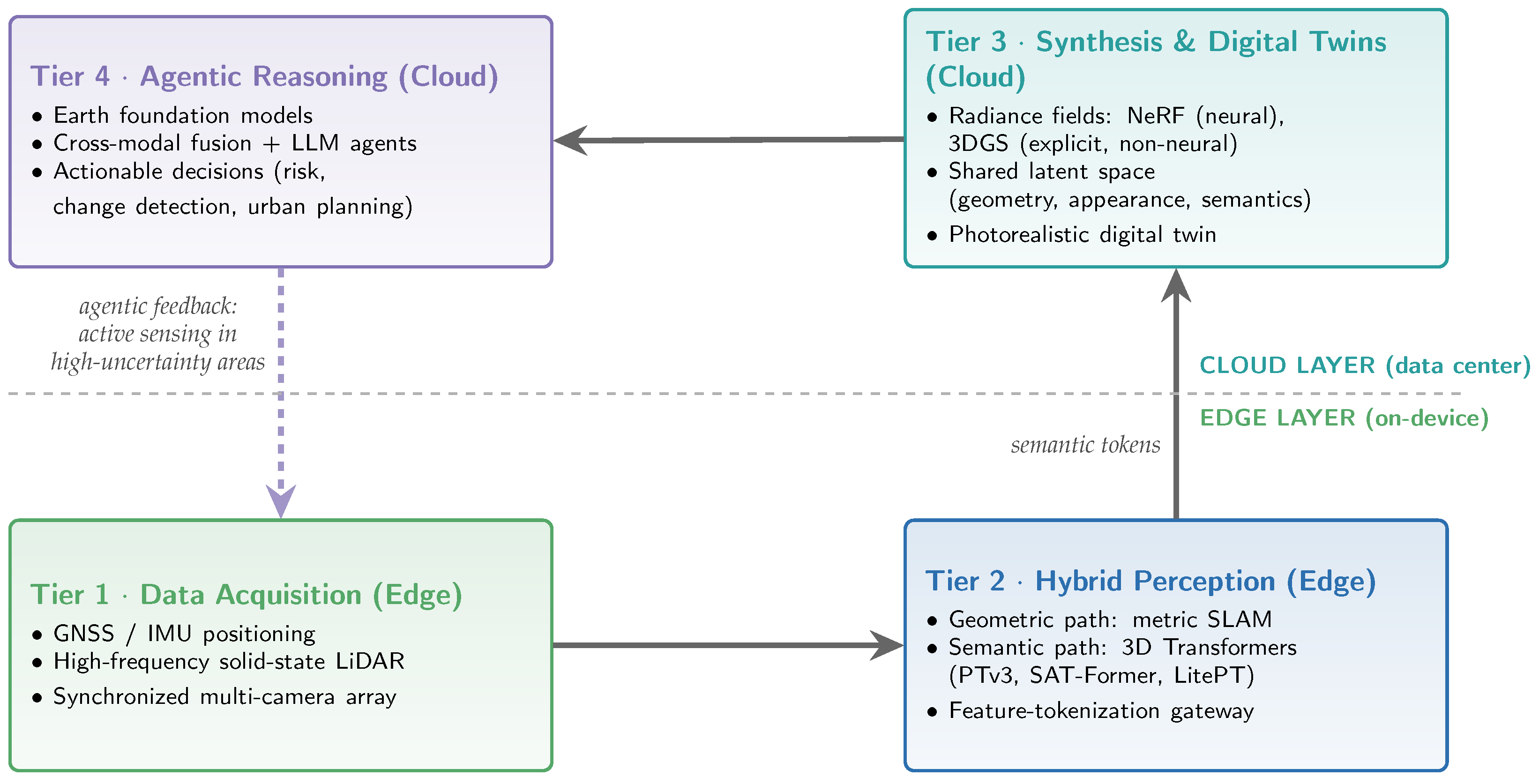
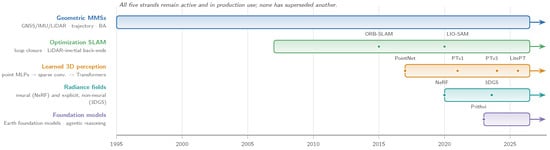
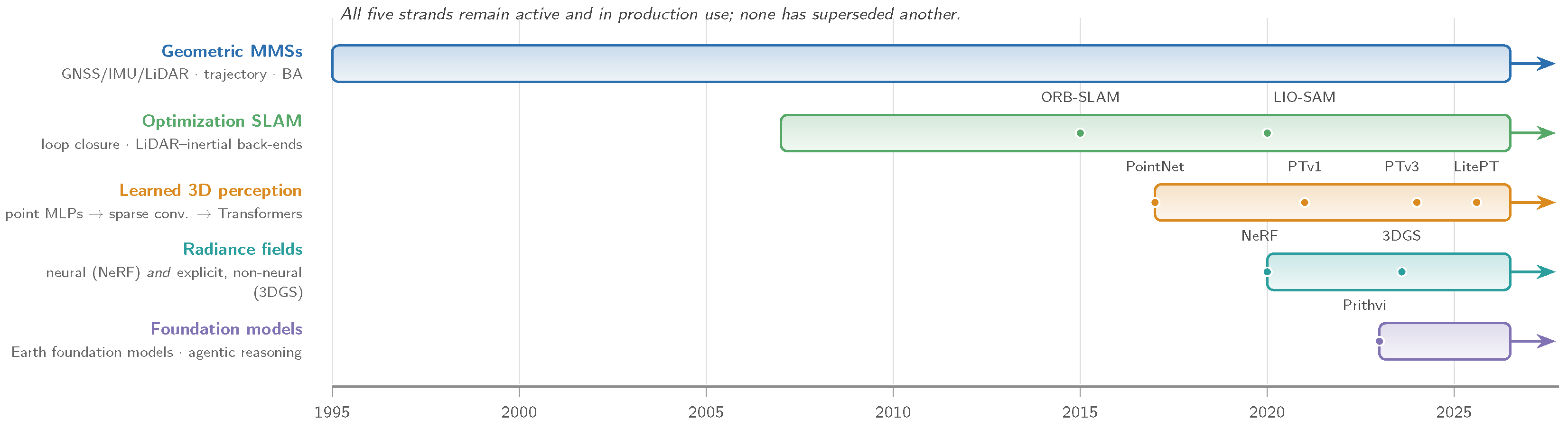
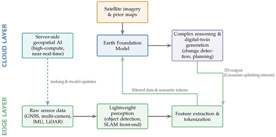
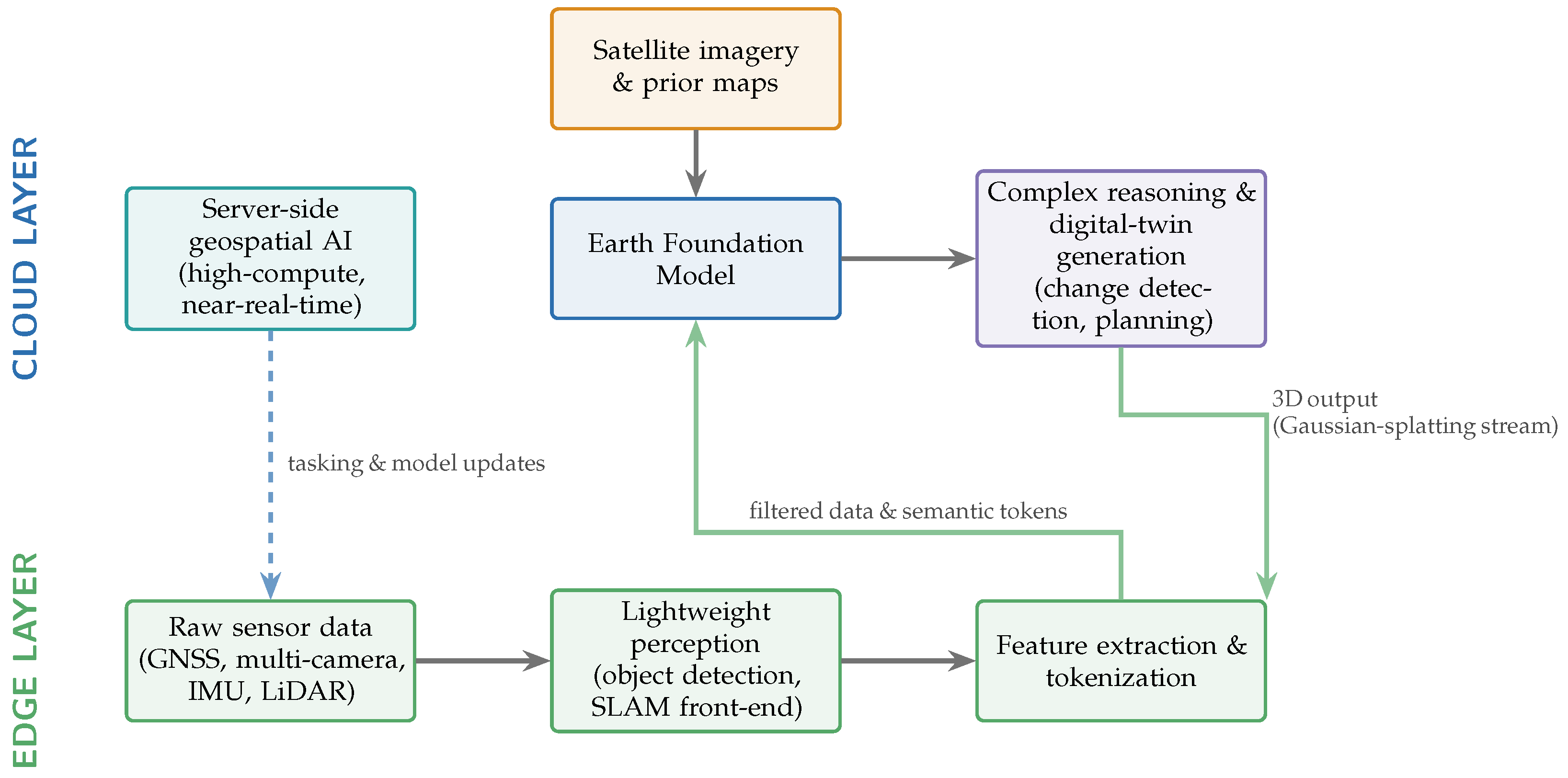
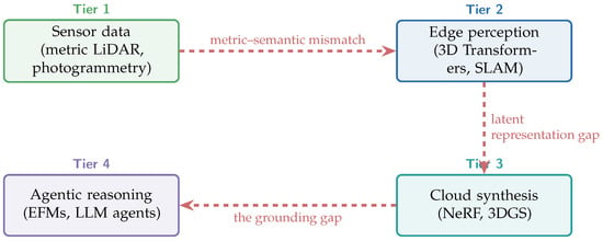
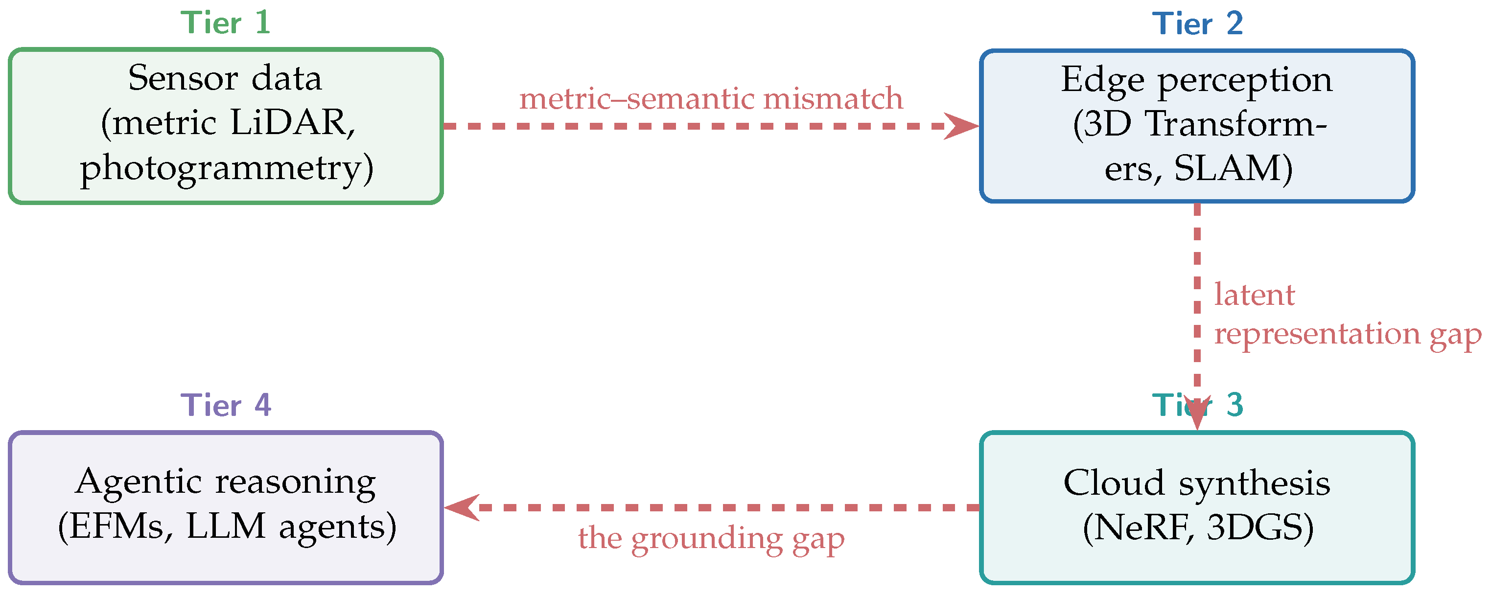

Disclaimer/Publisher’s Note: The statements, opinions and data contained in all publications are solely those of the individual author(s) and contributor(s) and not of MDPI and/or the editor(s). MDPI and/or the editor(s) disclaim responsibility for any injury to people or property resulting from any ideas, methods, instructions or products referred to in the content. |
© 2026 by the author. Licensee MDPI, Basel, Switzerland. This article is an open access article distributed under the terms and conditions of the Creative Commons Attribution (CC BY) license.