


Abstract
Coastal wetlands at urban margins experience interacting thermal, land-surface and hydrological pressures, yet composite remote-sensing assessments require transparent weighting, uncertainty analysis and careful interpretation. This study assessed late-autumn to early-winter environmental conditions across the 6.906 km2 Mai Po Marshes–Inner Deep Bay wetland system, Hong Kong, from 2000 to 2025. Landsat Collection 2 Tier 1 Level-2 scenes were harmonized into annual October–December composites to derive land-surface temperature, NDVI, MNDWI, NDBI, water-observation frequency and mapped aquatic area. The Relative Potential Hydrological Connectivity Index combined annual water frequency with proximity to persistent Inner Deep Bay open water, while the Wetland Environmental Stress Index integrated thermal stress, built-up pressure, vegetation deficit, moisture deficit and hydrological isolation using equal weights. Across 22 adequately observed years, NDVI increased significantly and MNDWI declined significantly. Mapped aquatic area also declined significantly, with a primary-threshold Theil–Sen slope of −0.04796 km2 per year. Full-series MNDWI sensitivity tests using thresholds of >0.00, >0.10 and >0.20 retained significant aquatic-area declines at all thresholds. In contrast, RPHCI showed no significant monotonic trend under any of the three MNDWI thresholds, and equal-weight WESI likewise showed no significant monotonic trend. Weighting sensitivity indicated stable annual rankings but substantial class changes under hydrology-emphasis weighting. The Landsat–MODIS temperature comparison showed poor agreement and was not treated as validation. Thus, WESI and RPHCI remain season-specific remote-sensing proxies rather than direct measures of annual ecological condition or hydraulic exchange within this wetland system.
1. Introduction
Wetlands regulate water storage, sediment and nutrient exchange, carbon cycling, flood attenuation and habitat provision across terrestrial and aquatic landscapes [1,2,3,4]. Coastal wetlands are particularly dynamic because their condition reflects interactions among freshwater inflow, tidal exchange, geomorphology, vegetation, sediment supply and human management. These functions can deteriorate when urban expansion, land reclamation, channel modification, pollution and climatic variability alter the distribution, movement and persistence of surface water [5,6,7]. Wetland loss can impair these services, and restoration does not necessarily recover all ecological functions [8].
Hydrological connectivity is central to wetland functioning because it governs the transfer of water, sediments, nutrients and organisms among channels, ponds, marshes and receiving waters [9,10]. Hydrological connectivity is not the same as the presence of water. A wet surface may remain isolated from a receiving water body, while a narrow channel may provide an important pathway even though it occupies a relatively small area. Remote-sensing studies that use only open-water or surface-moisture indices may therefore conflate water presence, water persistence and functional hydrological connectivity. Ecohydraulic assessments can help identify the hydraulic conditions needed to maintain estuarine shorebird habitat [11].
Urban development can also modify the surface-energy balance of wetland margins. Impervious materials generally have low moisture availability and reduced evaporative cooling, which can produce warmer daytime surface conditions than vegetated or water-rich surfaces [12,13,14]. Vegetation and surface water may moderate land-surface temperature, but relationships among thermal conditions, built-up expression and vegetation indices are not necessarily causal. They may also reflect land-cover differences, seasonal phenology, atmospheric conditions, mixed pixels and variations in image-acquisition timing. Urban expansion can also affect biodiversity and vegetation carbon pools [15].
Satellite remote sensing provides consistent spatial coverage for wetland systems in which long-term field observations are limited. The Normalized Difference Vegetation Index can represent vegetation greenness, the Modified Normalized Difference Water Index can enhance open-water and surface-moisture expression, and the Normalized Difference Built-up Index can indicate relative built-up or impervious-surface expression [7,16,17,18]. Landsat thermal products can also support land-surface temperature assessment at a spatial resolution suitable for heterogeneous urban–wetland environments. Long-term satellite archives have also been used to map global tidal-flat distribution and change [19].
These indices are well established and should not be presented as new methodological developments. The more important analytical challenge is to harmonize them through time, distinguish water occurrence from potential hydrological connectivity, document the assumptions used in constructing composite indices and avoid validating an index against variables that are already mathematically embedded within it. A correlation between a composite index and one of its components is partly predetermined by the index equation and cannot provide independent evidence of ecological validity.
Composite indicators may nevertheless be useful when several environmental dimensions must be summarized within a consistent framework. Their interpretation, however, depends on the choice of variables, normalization procedures, directional transformations, weighting coefficients and classification thresholds. Different defensible weights may preserve the rank ordering of observations while producing materially different index magnitudes or categorical assignments [20]. Transparent sensitivity analysis is therefore necessary whenever a composite index support environmental interpretation or management prioritization.
This study contributes applied and analytical insights rather than introducing new spectral indices. The study uses annual, seasonally harmonized Landsat observations for the period from 2000 to 2025 rather than inferring long-term change from a limited set of benchmark maps. It develops a transparent relative connectivity proxy based on proximity to Inner Deep Bay and annual water-observation frequency while explicitly avoiding claims that the proxy measures hydraulic exchange. It also constructs a Wetland Environmental Stress Index whose components, directions, normalization procedures and weights are clearly documented. The composite index is not presented as a direct measure of ecological vulnerability, biodiversity or ecosystem health.
The analysis examined how seasonal land-surface temperature, built-up expression, vegetation greenness and surface-water expression varied from 2000 to 2025. It also evaluated temporal changes in mapped aquatic extent and relative potential hydrological connectivity, determined whether equal-weight environmental stress showed a persistent trend or mainly episodic variability, and tested whether annual WESI rankings and classes were sensitive to alternative weighting choices. We interpreted statistical associations cautiously and did not infer causal relationships from observational satellite data alone.
2. Materials and Methods
2.1. Study Area
The study covered a 6.906-km2 analysis boundary across the Mai Po Marshes–Inner Deep Bay wetland system in north-western Hong Kong, adjacent to Shenzhen, China (Figure 1). The boundary included the principal wetland, tidal and pond environments, together with the adjoining urban–wetland transition needed to represent external land-surface pressures.
Figure 1.
Location of the 6.906 km2 Mai Po Marshes–Inner Deep Bay study area and Inner Deep Bay source zone in north-western Hong Kong. Coordinate labels were checked against the uploaded study-area geometry, which spans approximately 113.999–114.034° E and 22.471–22.504° N. The scale bar at 1 km integer intervals.
The wetland complex contains extensive intertidal mudflats, mangroves, reedbeds, traditionally managed gei wai, fishponds, tidal creeks and drainage channels. Inner Deep Bay is a shallow estuarine system influenced by tidal exchange and by freshwater and sediment inputs from Hong Kong and Shenzhen. Surface-water patterns vary with tidal stage, seasonal rainfall, pond-management practices, sluice operations, sedimentation and vegetation dynamics. The proximity of the wetland to a densely urbanized metropolitan corridor makes it suitable for examining the co-occurrence of surface-water expression, vegetation greenness, built-up pressure and land-surface temperature [21,22]. Research in the nearby Futian mangrove wetland has linked sediment mercury records to the industrial development of Hong Kong and Shenzhen [23].
2.2. Analytical Framework
The analytical framework separated annual satellite-image preparation, environmental-indicator generation, surface-water analysis, relative potential connectivity estimation, composite environmental-stress assessment, temporal trend analysis and independent satellite-product comparison. Google Earth Engine [24] was used for image preprocessing, quality masking, annual compositing, index calculation, water-frequency analysis and image export. Python 3.12 within Google Colab (cloud-based notebook environment; accessed in 2026) was used for statistical quality control, trend estimation, false-discovery-rate correction, weighting sensitivity, correlation analysis, chart production and table preparation.
We generated spatial products for the benchmark years 2000, 2010, 2020, and 2025 to support interpretation of representative spatial conditions. Temporal inference, however, was based on the complete annual series from 2000 to 2025. We treated the benchmark maps as supporting spatial evidence rather than the primary basis for long-term conclusions. The complete analytical workflow, from satellite-image preprocessing to environmental-indicator generation, relative potential connectivity assessment, WESI construction, statistical analysis and uncertainty evaluation is summarized in Figure 2.
Figure 2.
Analytical framework showing annual Landsat preprocessing, environmental-indicator calculation, water-frequency and aquatic-area estimation, relative potential hydrological-connectivity assessment, WESI construction, temporal trend analysis, weighting sensitivity and independent satellite-product comparisons. RPHCI is a remote-sensing proxy rather than a measure of hydraulic exchange, while WESI represents environmental stress rather than direct ecological condition.
2.3. Data Sources
The analysis used Landsat Collection 2 Level-2 imagery as the primary data source. The analysis included Landsat 5 Thematic Mapper, Landsat 7 Enhanced Thematic Mapper Plus, Landsat 8 Operational Land Imager and Thermal Infrared Sensor, and Landsat 9 Operational Land Imager-2 and Thermal Infrared Sensor-2 observations. We used MODIS MOD11A2 Version 6.1 for a cross-product comparison of daytime land-surface temperature, and JRC Global Surface Water Version 1.4 for a broad comparison of aquatic classifications. The datasets, spatial resolutions, analytical roles and quality-control procedures used in the study are summarized in Table 1.
Table 1.
Data sources and analytical roles.
For each year, we considered all Landsat scenes intersecting the analysis area be-tween 1 October and 31 December. This fixed late-autumn-to-early-winter window improves interannual seasonal comparability and reduces variation associated with the wetter part of the year. Hong Kong rainfall is concentrated mainly from spring through early autumn, while November and December are among the drier months [21,22]. Accordingly, all temporal conclusions in this study refer specifically to October–December surface conditions and should not be interpreted as annual wetland-integrity estimates. The compositing procedure did not standardize acquisition by tidal stage, pond-management schedule or sluice operation.
All available Landsat Collection 2 Tier 1 Level-2 scenes intersecting the analysis area between 1 October and 31 December were obtained for each year. The archive query returned 545 candidate scenes for 2000–2025: 117 Landsat 5 TM, 271 Landsat 7 ETM+, 113 Landsat 8 OLI/TIRS and 44 Landsat 9 OLI-2/TIRS-2 scenes. Landsat Collection 2 surface-reflectance values were converted using a multiplicative scale factor of 0.0000275 and an additive offset of −0.2. Surface temperature was calculated using a multiplicative scale factor of 0.00341802 and an additive term of 149.0 K, then converted to degrees Celsius. We removed clouds, cloud shadows, cirrus, snow, and fill pixels using QA_PIXEL, and excluded radiometrically saturated observations using QA_RADSAT. Optical validity was used for MNDWI, NDVI, NDBI, water-frequency and annual coverage calculations. Thermal validity was based on the native valid Landsat surface-temperature mask together with QA_PIXEL and QA_RADSAT; no additional ST_QA uncertainty or cloud-distance threshold was imposed in the final reproducible workflow.
A seasonal median composite was calculated for each year. Median compositing reduced the influence of residual clouds and anomalous observations. The number of valid MNDWI observations was retained for each pixel. Pixels with fewer than three valid observations were excluded from annual water-frequency and WESI calculations.
2.4. Environmental Indicators
Vegetation greenness was represented using the Normalized Difference Vegetation Index:
Surface-water and moisture expression were represented using the Modified Normalized Difference Water Index:
Relative built-up or impervious-surface expression was represented using the Normalized Difference Built-up Index:
Land-surface temperature was obtained from the USGS Collection 2 Level-2 surface-temperature product after applying the relevant scale factors and quality masks.
NDVI was interpreted as an indicator of vegetation greenness rather than a direct measure of biomass, vegetation productivity or ecological condition. MNDWI was interpreted as an indicator of open-water and surface moisture rather than a direct measure of water depth, soil moisture, or salinity. NDBI was treated as a relative indicator of built-up expression rather than a complete urban land-cover classification. Land-surface temperature represented the radiometric temperature of the surface and was not interpreted as water temperature or direct physiological thermal stress.
2.5. Annual Water-Observation Frequency
Each valid Landsat observation was classified as water when MNDWI exceeded 0.00. Annual water-observation frequency was calculated as the proportion of valid observations in which a pixel was classified as water
where WFi,y is the annual water-observation frequency for pixel i in year y, nw,i,y is the number of observations classified as water, and nv,i,y is the total number of valid observations.
A pixel was classified as part of the seasonal aquatic area when its water-observation frequency was at least 0.35, it had at least three valid observations and it belonged to a patch containing at least three connected 30 m pixels. The minimum-patch criterion reduced isolated classification noise. Water-frequency thresholds of 0.30 and 0.40 were also retained to test the sensitivity of the connectivity proxy to aquatic-classification choices. Supplementary Figure S1 presents the sensitivity of annual RPHCI estimates to the lower, primary, and upper water-frequency thresholds.
Because the per-observation MNDWI > 0.00 rule can include shallow turbid water, damp sediment and mixed shoreline pixels, an additional benchmark-year diagnostic was performed on the seasonal MNDWI composites using thresholds of >0.00, >0.10 and >0.20. For 2000, 2010, 2020 and 2025, respectively, the mapped areas above >0.00 were 3.932, 3.392, 3.028 and 2.382 km2; these declined to 3.568, 2.886, 2.758 and 2.041 km2 at >0.10 and to 3.252, 2.264, 2.492 and 1.778 km2 at >0.20 (Supplementary Table S1). This diagnostic is not a replacement for the observation-frequency classification because it operates on seasonal composite MNDWI rather than on every valid observation; it is reported to show the expected direction and magnitude of threshold sensitivity.
A full-series sensitivity analysis was additionally conducted across all 22 adequately observed years by repeating the per-observation classification at MNDWI thresholds of >0.00, >0.10 and >0.20. For each threshold, annual aquatic area, RPHCI and equal-weight WESI were recalculated and evaluated using Kendall’s tau and Theil–Sen slope. Supplementary Table S2 reports the results.
Annual mapped aquatic area was calculated by multiplying the number of aquatic pixels by the 30 m pixel area and converting the result to square kilometers.
2.6. Relative Potential Hydrological Connectivity Index
The hydrological source was defined reproducibly from JRC Global Surface Water Version 1.4. Persistent open water was identified as pixels with long-term water occurrence ≥90% within a 5 km search zone surrounding Mai Po; connected source patches smaller than 100 pixels were removed. This produced a 32.874 km2 persistent open-water source adjacent to Mai Po in Inner Deep Bay. The source is an analytical hydrological-source definition rather than an official administrative polygon. Euclidean distance from this source was calculated across the complete study area. Distance was converted to a relative-proximity score using
where Pi is the relative proximity of pixel i, di is its Euclidean distance from the Inner Deep Bay source, dmin is the minimum distance within the study area, and dmax is the maximum distance. Relative proximity therefore ranged from 0 (most distant) to 1 (nearest).
Pixel-level relative potential hydrological connectivity was calculated as the geometric mean of relative proximity and annual water-observation frequency:
The geometric mean required both terms to contribute to the final score. A location could not receive a high connectivity value solely because it was near Inner Deep Bay if it was rarely observed as water. Similarly, a frequently wet location could not receive the maximum score if it was situated far from the bay-facing source.
The annual Relative Potential Hydrological Connectivity Index was calculated as the aquatic-area-weighted mean of Ci,y across mapped aquatic pixels
where Ai is the area of the aquatic pixel i.
Hydrological isolation was calculated as the inverse of relative potential connectivity:
The RPHCI formulation was based on available satellite observations. It did not measure water discharge, flow direction, tidal exchange, hydraulic resistance, salinity transport, culvert operation, sluice management or subsurface connectivity. The term “relative potential connectivity” was therefore retained throughout the study.
2.7. Wetland Environmental Stress Index
The term ecological vulnerability was not used because the satellite variables did not directly measure biological condition, ecosystem sensitivity, adaptive capacity or ecological response. Instead, WESI was constructed to represent the co-occurrence of remotely observable environmental stressors. The five WESI components and their directions of increasing stress, analytical rationales and principal interpretive limitations are summarized in Table 2.
Table 2.
WESI components, stress directions and interpretive limits.
Thermal stress was normalized using fixed pooled limits of 24.1007 and 36.4688 °C. These values were the 2nd and 98th percentiles, respectively, of the pooled land-surface-temperature sample used to define cross-year normalization bounds. Percentile-based bounds were selected to limit the influence of isolated extreme observations while retaining a common scale for all years:
Built-up pressure was calculated by transforming NDBI from its theoretical range of –1 to 1 into a range of 0 to 1:
Vegetation deficit was calculated as the inverse of scaled NDVI:
Moisture deficit was calculated as the inverse of scaled MNDWI:
Hydrological isolation was represented by the inverse connectivity score:
All five components were therefore oriented so that larger values represented greater environmental stress. Equal weighting was selected as the primary formulation because no independently validated ecological evidence was available to justify privileging one component:
Annual mean WESI was calculated as:
where ny is the number of valid pixels in year y.
WESI values were divided into five fixed analytical classes for cross-year visual comparison. Values from 0.00 to less than 0.20 represented very low stress, values from 0.20 to less than 0.40 represented low stress, values from 0.40 to less than 0.60 represented moderate stress, values from 0.60 to less than 0.80 represented high stress, and values from 0.80 to 1.00 represented very high stress. These categories were analytical classes rather than ecological, regulatory or management thresholds.
2.8. Sensitivity Analysis of WESI Weighting
Two deterministic alternative WESI formulations were calculated to evaluate whether annual results depended strongly on the selected component weights. The hydrology-emphasis formulation assigned greater weight to hydrological isolation:
The urban–thermal-emphasis formulation assigned greater weights to thermal stress and built-up pressure:
Agreement between each alternative formulation and equal-weight WESI was evaluated using Spearman rank correlation, mean absolute difference, exact class agreement and quadratic-weighted Cohen’s kappa. Spearman correlation evaluated the stability of annual ordering, while mean absolute difference measured changes in continuous index magnitude. Exact class agreement and weighted kappa evaluated the stability of categorical interpretations. The exported spatial workflow also produced leave-one-component-out models and randomly perturbed weighting scenarios. These were used as supplementary uncertainty assessments and were not presented as alternative ecological truth models. Supplementary Figure S2 presents the results of the leave-one-component-out assess-ment and the Monte Carlo analysis based on 5000 randomly perturbed weighting com-binations.
2.9. Temporal Trend Analysis
Annual monotonic trends were evaluated using Kendall’s tau and the Theil–Sen slope [25]. Kendall’s tau measured the direction and strength of monotonic association with time, while the Theil–Sen estimator provided a robust median slope that was less sensitive to individual anomalous years than ordinary least-squares regression.
The Theil–Sen slope was expressed as
where Yi and Yj are observations recorded at times ti and tj.
A pre-specified adequate-coverage threshold of 80% was used to define the primary temporal series. Years below this threshold remained visible in the figures but were excluded from the primary trend tests. This prevented large areas of missing data from being interpreted as genuine environmental change. Benjamini–Hochberg false-discovery-rate correction was applied across the family of primary temporal tests. The procedure ranked the original p-values and controlled the expected proportion of false discoveries among statistically significant results [26].
Annual Spearman correlations were calculated only among the original variables and mapped aquatic area. WESI was not correlated with LST, NDBI, NDVI, MNDWI or hydrological isolation because those variables were already included in its formulation. Such component–index correlations would have been mathematically circular and could not provide independent evidence of environmental causation or ecological validity.
2.10. Independent Product Evaluation
Seasonal Landsat land-surface temperature was aggregated to the MODIS 1 km grid and compared with quality-screened MODIS MOD11A2 daytime land-surface temperature. The final matched dataset contained 14 co-located observations. Pearson’s correlation coefficient, mean bias, root-mean-square error and mean absolute error were calculated to assess cross-product correspondence.
The assessment was treated as a cross-product comparison rather than formal validation. Landsat and MODIS differ in spatial resolution, overpass time, viewing geometry, temporal compositing and thermal-retrieval procedures. The limited number of matched observations also prevented strong conclusions regarding systematic product accuracy. Supplementary Figure S3 presents the relationship between seasonal Landsat land-surface temperature and quality-screened MODIS MOD11A2 daytime land-surface temperature.
Landsat aquatic classifications were compared with JRC Global Surface Water observations at co-located sampled locations. The JRC dataset represents long-term historical water occurrence rather than year-specific October–December wetland conditions. The comparison therefore assessed broad cross-product correspondence rather than annual classification accuracy. Supplementary Figure S4 presents the distribution of JRC surface-water occurrence values across the Landsat aquatic and non-aquatic classes.
No independent biological, habitat-condition, water-quality or ecological-integrity dataset was available for the study period. WESI was consequently not validated as a measure of biodiversity status, ecosystem health or direct ecological condition.
3. Results
3.1. Benchmark Spatial Patterns
Figure 3 presents benchmark spatial products for 2000, 2010, 2020, and 2025. The maps show the spatial distribution of the seasonal aquatic mask, relative potential hydrological connectivity and equal-weight WESI. Classified aquatic surfaces became less extensive in later benchmark years, while connectivity remained strongest where frequent seasonal water observations coincided with greater proximity to Inner Deep Bay. Equal-weight WESI was spatially heterogeneous in every benchmark year, demonstrating that the study-area mean did not represent uniform conditions across the wetland.
Figure 3.
Benchmark spatial products for 2000, 2010, 2020 and 2025. Rows show the seasonal aquatic mask, pixel-level relative potential hydrological connectivity, and equal-weight WESI. These maps provide representative spatial context; long-term inference is based on the complete, well-observed annual series rather than the four benchmark years alone.
3.2. Observation Availability and Coverage
As shown in Figure 4, the Landsat Collection 2 Tier 1 Level-2 archive contained 545 candidate scenes intersecting the study area during the October–December observation periods from 2000 to 2025. These comprised 117 Landsat 5 TM, 271 Landsat 7 ETM+, 113 Landsat 8 OLI/TIRS and 44 Landsat 9 OLI-2/TIRS-2 scenes. Annual candidate-scene counts ranged from 10 to 33. Pixel-level QA screening was then applied before annual compositing. Most years provided nearly complete spatial coverage of the 6.906 km2 study area, and the proportion satisfying the minimum requirement of at least three valid observations ranged from 0.061 to 0.997.
Figure 4.
Annual observation availability and environmental indicators across the Mai Po Marshes–Inner Deep Bay wetland system from 2000 to 2025. Panels show (a) the fraction of the study area with at least three valid observations, (b) annual Landsat scene count, (c) mean land-surface temperature (LST), (d) mean NDVI, (e) mean MNDWI and (f) mean NDBI. Solid blue lines with circular markers connect annual observa-tions. Cross symbols identify 2011, 2012, 2015 and 2016, which had <80% adequate spatial cov-erage and were excluded from the primary trend analysis. The horizontal blue dashed line in panel (a) marks the 80% coverage threshold. Orange dashed lines in panels (c–f) show Theil–Sen trends estimated using adequately observed years.
Figure 4 also identifies the four years that failed to meet the pre-specified 80% adequate-coverage threshold. Adequate coverage was 0.489 in 2011, 0.061 in 2012, 0.750 in 2015 and 0.780 in 2016. These years were excluded from the primary trend analyses, reducing the principal temporal dataset to 22 adequately observed years. We retained them in the annual plots and marked them separately to show how incomplete spatial coverage affected the estimated environmental indicators.
Coverage was most limited in 2012, when only 6.1% of the study area met the minimum observation requirement. Consequently, the unusually small aquatic-area estimate and low connectivity value recorded for that year were interpreted as consequences of insufficient observation coverage rather than genuine system-wide environmental change. The coverage panel in Figure 4 therefore provides an essential basis for interpreting the annual indicator series and distinguishing observational anomalies from environmental signals.
3.3. Environmental-Indicator Trends
Figure 4 shows substantial interannual variation in mean October–December land-surface temperature, with particularly warm seasonal composites in 2014 and 2018. Both years met the pre-specified coverage criterion: adequate-coverage fractions were 0.997 in 2014 and 0.983 in 2018. They were therefore retained in the primary trend analysis. In contrast, 2011, 2012, 2015 and 2016 were excluded because their adequate-coverage fractions were below 0.80. The annual series did not exhibit a statistically significant monotonic trend.
The annual NDBI series in Figure 4 also showed no statistically significant monotonic trend. As summarized in Table 3, Kendall’s tau was −0.264 and the Theil–Sen slope was −0.00142 per year. The 95% confidence interval extended from −0.00295 to 0.00044 per year, while the FDR-adjusted p-value was 0.136. Although the negative slope suggested a weak decline in mean built-up spectral expression, the confidence interval included zero and the trend was not statistically significant after correction for multiple testing.
Table 3.
Selected primary annual trend results after excluding years with less than 80% adequate spatial coverage.
In contrast, the NDVI panel in Figure 4 displays a clear upward trajectory. Mean NDVI increased significantly, with Kendall’s tau of 0.636 and a Theil–Sen slope of 0.00440 per year. The 95% confidence interval ranged from 0.00279 to 0.00579 per year, while the FDR-adjusted p-value was less than 0.001. This result indicated a sustained increase in seasonal vegetation greenness across the adequately observed years. However, the trend represents increasing spectral greenness rather than direct evidence of increasing bio-mass, primary productivity, habitat quality or ecosystem health.
The MNDWI series in Figure 4 exhibited the opposite temporal pattern. Kendall’s tau was −0.472 and the Theil–Sen slope was −0.00491 per year. The 95% confidence interval ranged from −0.00760 to −0.00198 per year, and the FDR-adjusted p-value was 0.005. The statistically significant decline therefore indicated a long-term reduction in seasonal open-water and surface-moisture expression within the study area.
Taken together, the indicator panels in Figure 4 and the trend statistics reported above demonstrate that increasing vegetation greenness occurred simultaneously with declining open-water and surface-moisture expression. The opposing NDVI and MNDWI trends indicate that vegetation and surface-water conditions represented distinct dimensions of wetland change rather than a single unidirectional environmental response.
3.4. Mapped Aquatic-Area Change
The mapped seasonal aquatic-area series shows a substantial decline between 2000 and 2025. Aquatic extent decreased from approximately 3.995 km2 in 2000 to 2.591 km2 in 2025, an endpoint reduction of approximately 1.404 km2. The largest adequately observed aquatic extent was approximately 4.174 km2 in 2005.
After excluding the four low-coverage years, mapped aquatic area showed a strong and statistically significant monotonic decline. Kendall’s tau was −0.749 and the Theil–Sen slope was −0.04796 km2 per year (95% CI: −0.05743 to −0.03925 km2 per year; unadjusted p < 0.001). Full-series sensitivity analysis confirmed significant declines under MNDWI thresholds >0.10 and >0.20 (Supplementary Table S2). This was the strongest long-term temporal signal identified among the primary environmental indicators.
Figure 5 also shows the exceptionally low aquatic-area estimate of approximately 0.194 km2 in 2012. However, Figure 4 demonstrates that only 6.1% of the study area had adequate observation coverage in that year. The 2012 value was therefore treated as an observation anomaly rather than evidence of a genuine wetland-wide contraction and was excluded from the primary trend calculation.
Figure 5.
Temporal variation in mapped aquatic area and WESI results. The figure presents annual mapped aquatic area, the equal-weight, hydrology-emphasis and urban–thermal-emphasis WESI formula-tions, annual area with WESI values of at least 0.60, and the rank-correlation and class-agreement statistics for the alternative weighting formulations. In the annual time-series panels, solid lines connect observed annual values and dashed lines show Theil–Sen trends where plotted. For WESI formulations, blue denotes equal-weight WESI, orange denotes hydrology-emphasis WESI and green denotes urban–thermal-emphasis WESI. Cross symbols identify years excluded from pri-mary trend tests because adequate spatial coverage was below 80%.
The declining aquatic-area trajectory shown in Figure 5 was consistent with the significant reduction in MNDWI reported in Figure 4 and Table 3. Together, these results indicate that both the spatial extent of classified aquatic surfaces and the average spectral expression of open water and surface moisture declined over the study period. Nevertheless, the satellite observations alone could not determine whether the contraction resulted from vegetation colonization, sediment accumulation, pond-management practices, tidal variability, reduced seasonal inundation or physical hydrological modification.
3.5. Relative Potential Hydrological Connectivity
The benchmark connectivity surfaces generated for 2000, 2010, 2020 and 2025 showed a persistent spatial gradient across the Mai Po–Inner Deep Bay wetland system. Higher RPHCI values occurred where frequent seasonal water observations coincided with greater proximity to Inner Deep Bay. Lower values occurred in locations that were farther from the bay-facing source, less frequently observed as water, or characterized by both conditions. Hydrological isolation exhibited the inverse pattern, with frequently wet bay-facing surfaces showing lower isolation than drier or more distant areas.
Using the final reproducible persistent open-water source, RPHCI did not show a statistically significant monotonic trend over the 22 adequately observed years. At the primary MNDWI threshold (>0.00), Kendall’s tau was 0.048 and the Theil–Sen slope was +0.000155 per year (95% CI: −0.000618 to +0.000820; unadjusted p = 0.781). Full-series MNDWI threshold sensitivity produced the same inference at >0.10 (tau = 0.030, slope = +0.000122 per year, p = 0.867) and >0.20 (tau = 0.195, slope = +0.000687 per year, p = 0.217). Thus, the data do not support a persistent directional change in the relative potential-connectivity proxy.
Annual RPHCI was approximately 0.698 in 2000 and 0.696 in 2025 at the primary MNDWI threshold. Interannual variation was present, but the endpoint similarity and non-significant monotonic trend indicate that the final RPHCI series should be interpreted as broadly stable through time rather than as evidence of systematic connectivity decline.
RPHCI varied alongside changes in MNDWI, annual water-observation frequency and mapped aquatic area, but it did not share their significant long-term decline in the final analysis. These indicators represent related but distinct properties. MNDWI represents the spectral expression of open water and surface moisture, mapped aquatic area represents the extent satisfying the selected classification criteria, and RPHCI integrates water-observation frequency with relative proximity to persistent Inner Deep Bay open water.
Supplementary Figure S1 demonstrates that annual RPHCI values varied moderately when the aquatic water-frequency threshold was changed from the primary value of 0.35 to the lower and upper alternatives of 0.30 and 0.40. This sensitivity confirms that the magnitude of the connectivity proxy depended partly on the threshold used to define seasonally aquatic surfaces.
The RPHCI time series should not be interpreted as direct evidence of hydraulic exchange or hydrological disconnection. RPHCI is a relative remote-sensing proxy and does not measure water discharge, tidal exchange, flow direction, water depth, channel capacity, hydraulic resistance, sluice operation, culvert performance or subsurface connectivity. The results therefore characterize relative potential for observable surface-water linkage rather than physical water movement.
3.6. WESI Temporal Behavior
The WESI time series shows considerable interannual variation but no consistent long-term increase. Mean equal-weight WESI was approximately 0.416 in 2000 and 0.401 in 2025. Across the 22 adequately observed years, Kendall’s tau was 0.074 and the Theil–Sen slope was +0.000442 per year (95% CI: −0.001731 to +0.001906; unadjusted p = 0.656). The trend was therefore not statistically significant. Full-series MNDWI-threshold sensitivity produced the same non-significant inference at >0.10 and >0.20 (Supplementary Table S2).
The annual WESI series indicates that environmental stress was episodic rather than continuously increasing. Among the 22 adequately observed years, the highest mean equal-weight WESI occurred in 2014 (approximately 0.466), followed by 2018 (approximately 0.441). These peaks reflect years in which several remotely observed stress dimensions coincided.
The WESI area panel in Figure 5 similarly shows no persistent increase in the area classified at or above 0.60. The corresponding trend statistics indicate that Kendall’s tau was 0.045 and the Theil–Sen slope was effectively 0.00000 km2 per year. The 95% confidence interval ranged from −0.00053 to 0.00120 km2 per year, while the FDR-adjusted p-value was 0.871. However, episodic expansions of the higher-stress area occurred in 2014 and 2018, when approximately 0.395 km2 and 0.295 km2, respectively, exceeded the 0.60 threshold.
The combined evidence from Figure 5 and the trend statistics above therefore does not support an interpretation of steadily increasing system-wide environmental stress. Instead, elevated WESI values occurred during particular years when several remotely observed stress dimensions coincided. The annual study-area mean also concealed spatial variation because localized areas of elevated stress could occur even when the overall mean remained within the low or moderate analytical classes.
3.7. Weighting Sensitivity Results
Figure 5 compares the annual equal-weight, hydrology-emphasis and urban–thermal-emphasis WESI formulations. Although the three series generally followed similar temporal patterns, the quantitative sensitivity statistics in Table 4 show that changes in component weights affected both continuous index values and categorical assignments.
Table 4.
WESI sensitivity and independent-product assessment.
The hydrology-emphasis formulation was strongly associated with equal-weight WESI, with a Spearman correlation of 0.941. Table 4 shows that the mean absolute difference between the two formulations was 0.069. Despite the strong rank agreement, exact class agreement was only 19.2%, and quadratic-weighted Cohen’s kappa was 0.022. Increasing the weight assigned to hydrological isolation therefore changed the stress category assigned to most years even though the relative ordering of years remained broadly stable.
The urban–thermal-emphasis formulation also maintained a strong relationship with equal-weight WESI, with a Spearman correlation of 0.906. As reported in Table 4, its mean absolute difference was 0.068, exact class agreement was 96.2% and quadratic-weighted Cohen’s kappa was 0.780. The categorical results were therefore considerably more stable when thermal stress and built-up pressure were emphasized than when hydrological isolation received greater weight.
Table 3 also shows that the hydrology-emphasis WESI had a positive Theil–Sen slope of 0.00227 per year, with a 95% confidence interval ranging from 0.00039 to 0.00353 per year. Although the unadjusted test was statistically significant, the FDR-adjusted p-value was 0.056. The trend was therefore not considered statistically significant after correction for multiple comparisons.
The leave-one-component-out results presented in Supplementary Figure S2 demonstrate that WESI was most sensitive to the removal of hydrological isolation. Omitting hydrological isolation produced the lowest Spearman correlation with the complete equal-weight formulation, at 0.656, and the largest mean absolute difference, at approximately 0.091. Exact class agreement was approximately 62.8%, while quadratic-weighted Cohen’s kappa was 0.126. By comparison, omitting built-up pressure produced a Spearman correlation of 0.984 and a mean absolute difference of approximately 0.023.
Supplementary Figure S2 also presents the results of the 5000-scenario Monte Carlo weighting analysis. The median Spearman correlation with equal-weight WESI was approximately 0.996, with a 95% interval ranging from 0.960 to 1.000. The median mean absolute difference was approximately 0.017, with a 95% interval ranging from 0.004 to 0.047. These results indicate that continuous WESI rankings were generally robust to moderate random changes in the component weights.
The results shown in Figure 5, Table 4 and Supplementary Figure S2 demonstrate that rank stability did not necessarily imply categorical stability. Equal weighting was therefore retained as a transparent reference formulation rather than treated as an objectively correct ecological weighting system.
3.8. Non-Circular Environmental Associations
Figure 6 presents the Spearman correlation matrix for the original annual environmental indicators and mapped aquatic area. WESI was deliberately excluded because LST, NDBI, NDVI, MNDWI and hydrological isolation were already mathematically embedded within its formulation. Correlating WESI with these components would have produced partly predetermined relationships and would not have constituted independent validation.
Figure 6.
Spearman correlation matrix for original annual environmental variables and mapped aquatic area after excluding years with less than 80% adequate spatial coverage. WESI was excluded because its component variables are mathematically embedded in the index. Asterisks indicate statistical significance after false-discovery-rate correction: p < 0.05 (*), p < 0.01 (**), and p < 0.001 (***).
As shown in Figure 6, mean annual MNDWI was strongly and positively associated with mapped aquatic area. The Spearman correlation was 0.798, and the FDR-adjusted p-value was less than 0.001. Years with stronger open-water and surface-moisture expression therefore generally contained larger mapped aquatic extents.
Figure 6 also shows a strong negative association between NDVI and mapped aquatic area. The Spearman correlation was −0.787, and the FDR-adjusted p-value was less than 0.001. NDVI was additionally negatively related to MNDWI, with a Spearman correlation of −0.659 and an FDR-adjusted p-value of 0.0028. These results indicated that years characterized by greater vegetation greenness commonly had lower open-water expression and smaller mapped aquatic areas.
The relationships shown in Figure 6 did not establish causal direction. Increasing vegetation greenness may reflect colonization of formerly open or shallow-water surfaces, but declining aquatic extent could also have resulted from water-level management, sediment accumulation, tidal variability or another common environmental process. The correlations therefore represented temporal associations rather than evidence that vegetation change directly caused aquatic-area contraction.
Mean land-surface temperature showed no statistically significant FDR-adjusted relationship with NDVI, MNDWI, NDBI or mapped aquatic area. The LST–NDVI correlation was 0.187, the LST–MNDWI correlation was −0.339, the LST–NDBI correlation was 0.290 and the LST–aquatic-area correlation was −0.231. NDBI was also not significantly related to NDVI, MNDWI or aquatic area after FDR correction. Figure 6 therefore demonstrates that the strongest annual relationships were concentrated among vegetation greenness, surface-water expression and mapped aquatic extent rather than thermal or built-up conditions.
The Landsat–MODIS land-surface-temperature comparison presented in Supplementary Figure S3 was based on 14 co-located observations after seasonal Landsat values were aggregated to the MODIS 1 km spatial resolution. The comparison yielded a strong negative Pearson correlation of −0.885 (p < 0.001). Landsat land-surface temperature was, on average, 1.30 °C higher than the corresponding MODIS daytime land-surface temperature. The root-mean-square error was 3.01 °C, while the mean absolute error was 2.59 °C.
The scatter plot in Supplementary Figure S3 shows that the matched Landsat and MODIS observations did not reproduce a consistent common temperature pattern. The strong negative relationship and relatively large error statistics therefore indicated poor cross-product agreement within the limited matched sample. The comparison was not used to validate Landsat land-surface temperature, the thermal-stress component of WESI or the final environmental-stress index.
3.9. Independent Product Comparisons
Several factors may have contributed to the disagreement shown in Supplementary Figure S3, including differences in satellite overpass time, spatial resolution, viewing geometry, seasonal compositing, thermal-retrieval procedures and pixel composition. The heterogeneous Mai Po landscape contains open water, mudflats, vegetation, fishponds and developed surfaces, which may be represented separately in Landsat imagery but combined within a single MODIS pixel. The sample size of only 14 matched observations further limited the strength of any validation inference.
Supplementary Figure S4 compares Landsat aquatic classifications with JRC Global Surface Water observations at co-located sampled locations. Among 4804 sampled Landsat aquatic observations, 53.4% coincided with JRC historical water occurrence of at least 75%, and 30.5% coincided with occurrence of at least 90%. These percentages indicate substantial overlap with historically persistent water but do not distinguish tidal mudflats from permanent channels, gei wai or fishponds. No independent habitat-type mask with consistent 2000–2025 coverage was available; therefore, we did not infer a numerical tidal-flat fraction from spectral water occurrence alone.
The independent-product results summarized in Table 4 and illustrated in Supplementary Figures S3 and S4 were therefore interpreted as cross-product comparisons rather than formal ecological validation. No independent biological, water-quality, habitat-condition or ecological-integrity observations were available for the study period. WESI consequently remained a remote-sensing environmental-stress proxy, while RPHCI remained a relative potential-connectivity proxy rather than a validated measure of ecosystem condition or hydraulic exchange.
4. Discussion
4.1. Concurrent Vegetation Greening and Declining Surface-Water Expression
The strongest long-term results were increased NDVI, declining MNDWI, and contraction of mapped aquatic area. These changes should not be reduced to a simple narrative of environmental improvement or degradation. Increasing NDVI may reflect vegetation expansion, denser canopy development, mangrove or reed growth, seasonal phenological differences or vegetation colonization of formerly open or shallow-water environments.
Declining MNDWI and mapped aquatic area indicated reduced seasonal expression of open water within the analysis boundary. The strong negative association between NDVI and aquatic area supported the coexistence of vegetation greening and reduced open-water extent. However, the association did not reveal the direction of causation.
The combination of vegetation greening and aquatic-area contraction may arise through several processes. Vegetation may expand into shallow-water or exposed-sediment environments as water levels decline. Sediment accumulation may create conditions suitable for vegetation establishment. Managed pond conditions may alter the balance between open water and vegetated surfaces. Ecological succession, hydrological modification, and changes in seasonal inundation may also contribute [21].
Spectral indicators require contextual interpretation because they respond to several surface properties. NDVI is influenced by vegetation type, canopy structure, phenology and the presence of water or exposed sediment beneath vegetation. MNDWI may vary with turbidity, mixed pixels, exposed sediment, built surfaces and atmospheric conditions [7,16,17,27].
These alternative mechanisms are consistent with the broader wetland remote-sensing literature, which emphasizes that spectral change can reflect vegetation succession, hydrological variation, sediment exposure and mixed land–water pixels rather than a single ecological process [28,29]. Historical habitat maps, field vegetation surveys, pond-management records, sediment measurements, water-level observations and information on sluice operations would therefore be useful for discriminating among mechanisms.
4.2. Thermal Variability Without a Persistent Monotonic Trend
Annual land-surface temperature varied substantially, and relatively high values occurred in 2014 and 2018. However, the complete primary series did not show a significant monotonic trend. This finding did not support a claim that system-wide thermal stress continuously intensified from 2000 to 2025.
Instead, the results indicated that elevated thermal conditions were episodic during the October–December observation window. Urban, impervious and exposed surfaces commonly have higher daytime LST than vegetated or water-rich surfaces because they have lower evapotranspiration and different heat-storage and radiative properties [12,13].
Annual mean LST is nevertheless affected by seasonal weather conditions, atmospheric screening, image-acquisition timing, surface moisture, tidal exposure and the location of valid observations. A warm annual composite may therefore reflect a combination of environmental conditions rather than a persistent structural change.
The absence of a system-wide monotonic trend does not mean that localized thermal contrasts are environmentally unimportant. Built-up margins, exposed pond substrates and dry surfaces may still experience substantially warmer conditions than adjacent water-rich or vegetated areas. The result means only that the annual study-area mean did not support a claim of continuous thermal increase.
4.3. Aquatic-Area Contraction and Relative Potential Hydrological Connectivity
The significant contraction of mapped aquatic area represented the clearest long-term environmental change identified within the Mai Po–Inner Deep Bay wetland system. After excluding years with inadequate spatial coverage, mapped aquatic area declined at a Theil–Sen rate of 0.04796 km2 per year under the primary MNDWI >0.00 threshold. Full-series sensitivity analysis confirmed significant declines at MNDWI thresholds >0.10 (−0.03933 km2 per year, p < 0.001) and >0.20 (−0.03161 km2 per year, p = 0.0048). The magnitude of mapped aquatic extent therefore depended on threshold choice, but the inference of long-term contraction was robust across all three thresholds. This decrease was accompanied by a significant decline in MNDWI, indicating a broader weakening of seasonal open-water and surface-moisture expression. The satellite-derived trend alone cannot determine whether the observed decline resulted from sedimentation, vegetation colonization, pond-management practices, reduced inundation, hydrological modification or changing seasonal water levels.
The Relative Potential Hydrological Connectivity Index provided complementary information by representing the joint occurrence of seasonal surface-water observations and spatial proximity to persistent Inner Deep Bay open water. In the final reproducible analysis, RPHCI showed no significant monotonic trend during the 22 adequately observed years (Kendall’s tau = 0.048; Theil–Sen slope = +0.000155 per year; 95% CI: −0.000618 to +0.000820; unadjusted p = 0.781). Full-series MNDWI-threshold sensitivity likewise yielded non-significant RPHCI trends at >0.10 and >0.20.
The RPHCI results indicate interannual variability without a persistent monotonic change in the seasonal co-occurrence of frequently observed surface water and proximity to the bay-facing persistent-water source. This differs from the significant decline in mapped aquatic area and MNDWI, underscoring that spectral water expression, mapped aquatic extent and relative potential connectivity are related but analytically distinct dimensions of the wetland system.
Hydrological connectivity is a multidimensional property involving the transfer of water, sediments, nutrients, energy and organisms among aquatic and wetland environments [9,10]. Connectivity is therefore not equivalent to the simple presence of surface water. A wet surface may remain hydraulically isolated, while a narrow channel may provide an important pathway despite occupying a relatively small area. Remote-sensing indicators based solely on spectral water detection may therefore fail to distinguish water presence, water persistence and functional hydraulic exchange [28,30].
The present RPHCI formulation represented only the relative potential surface-water linkage under the available satellite observations. It did not measure discharge, water velocity, tidal exchange, flow direction, channel capacity, hydraulic resistance, sluice operation, culvert performance, salinity transport or subsurface connectivity. Consequently, a location could have a low RPHCI value even where managed or subsurface water exchange remained active. Conversely, a frequently wet and bay-facing location could receive a relatively high RPHCI value without evidence of strong hydraulic flow. RPHCI should therefore be interpreted as a remote-sensing screening proxy rather than a direct hydrodynamic measurement.
The continuous formulation, nevertheless, provided a useful analytical advantage because it avoided treating every small gap in a binary water classification as a complete hydrological barrier. It allowed potential connectivity to vary gradually according to both water persistence and relative location. This approach is appropriate for heterogeneous wetlands where open water, vegetated marshes, fishponds, tidal channels and managed structures occur within a spatially complex landscape [28,29].
Areas characterized by consistently low RPHCI and high hydrological isolation may warrant field investigation for sediment accumulation, channel obstruction, weak pond exchange or changes in managed water conditions. Confirm these interpretations using water-level records, channel surveys, sluice-operation information, and hydrodynamic measurements before proposing restoration, dredging, or water-management interventions. The water-frequency threshold assessment presented in Supplementary Figure S1 demonstrates that the magnitude of RPHCI depends partly on the threshold used to define seasonal aquatic surfaces. This result reinforces the interpretation of RPHCI as a relative and method-dependent remote-sensing proxy rather than a direct measurement of hydraulic exchange.
4.4. WESI Robustness and Weighting Dependence
The equal-weight Wetland Environmental Stress Index showed a statistically significant monotonic trend from 2000 to 2025. The Theil–Sen slope was 0.00104 per year, while the FDR-adjusted p-value was 0.229. This result indicates that the combined environmental-stress signal was characterized more strongly by interannual variability and episodic peaks than by a continuous long-term increase. The highest mean WESI values occurred in 2014 and 2018, when relatively warm surface conditions coincided with combinations of reduced moisture expression, vegetation conditions, built-up pressure and hydrological isolation.
The absence of a significant system-wide trend does not imply that environmental stress was absent or spatially uniform. Wetland systems may be exposed simultaneously to hydrological modification, urban development, altered vegetation, pollution and thermal pressures, but the magnitude and spatial distribution of these stressors may vary substantially through time [5,31]. Urban and impervious surfaces may also modify surface-energy conditions and contribute to elevated land-surface temperatures, particularly at wetland margins where water-rich, vegetated and developed surfaces occur in proximity [12,13,14].
WESI summarized five remotely observable dimensions of environmental conditions: thermal stress, built-up pressure, vegetation deficit, moisture deficit and hydrological isolation. A relatively low annual mean could conceal localized areas with elevated stress, while a high annual value could result from different combinations of component conditions. Two locations with identical WESI values may therefore have substantially different environmental characteristics. Always examine the component maps alongside the composite index rather than interpreting WESI as a complete ecological diagnosis.
The deterministic weighting analysis demonstrated an important distinction between the stability of annual rankings and the stability of categorical stress assignments. The hydrology-emphasis formulation correlated strongly with the equal-weight model (Spearman’s ρ = 0.941). However, its mean absolute difference from the equal-weight formulation was 0.069, while exact class agreement was only 19.2%. Quadratic-weighted Cohen’s kappa was 0.022, indicating very weak categorical agreement. Thus, years that remained similarly ordered from relatively low to relatively high stress were frequently reassigned to different analytical classes when greater importance was assigned to hydrological isolation.
The urban–thermal-emphasis formulation also preserved the annual ordering of environmental stress, with a Spearman correlation of 0.906 relative to equal-weight WESI. The mean absolute difference was 0.068. In contrast to the hydrology-emphasis model, exact class agreement reached 96.2%, while quadratic-weighted Cohen’s kappa was 0.780. The categorical results were therefore considerably more stable when the weights assigned to thermal stress and built-up pressure were increased than when hydrological isolation received greater emphasis.
These findings show that a strong rank correlation between two composite-index formulations does not necessarily mean that their categorical interpretations are equivalent. Small changes in continuous values may move observations across fixed class boundaries while leaving the overall ordering largely unchanged. Composite indicators are inherently influenced by decisions concerning variable selection, normalization, directional transformation, weighting and classification thresholds [20]. Stress categories should therefore not be treated as objective ecological thresholds when they have not been calibrated using independent environmental or biological observations.
The leave-one-component-out analysis provided additional evidence that hydrological isolation exerted an important influence on WESI behavior. Omitting hydrological isolation produced the lowest rank agreement with the complete equal-weight formulation, with a Spearman correlation of 0.656. It also produced the largest mean absolute difference (approximately 0.091) and a quadratic-weighted kappa of only 0.126. In contrast, omitting built-up pressure produced a Spearman correlation of 0.984 and a substantially smaller mean absolute difference of approximately 0.023.
The relatively strong influence of hydrological isolation should not be interpreted as proof that it was objectively the most ecologically important stressor. Its influence reflects WESI’s mathematical structure and the variability of the input component. No independent ecological observations were available to determine an optimal or biologically validated set of component weights. We therefore retained equal weighting as a transparent reference formulation rather than presenting it as an objectively correct ecological model.
The Monte Carlo analysis showed stronger overall stability under randomly perturbed weighting combinations. Across 5000 weighting scenarios, the median Spearman correlation with equal-weight WESI was approximately 0.996, with a 95% interval ranging from 0.960 to 1.000. The median mean absolute difference was approximately 0.017, with a 95% interval from 0.004 to 0.047. These results indicate that continuous WESI rankings were generally robust to moderate random changes in the weights. Nevertheless, the deterministic hydrology-emphasis scenario demonstrated that targeted increases in a particular component could materially alter categorical assignments.
The results support reporting continuous WESI values, individual component layers and alternative weighting scenarios alongside categorical maps. Management conclusions should not be based solely on whether a location falls within a very low, low, moderate, high or very high WESI class. Greater confidence may be placed in locations that consistently show elevated values under several weighting formulations and that are independently supported by field evidence on water quality, habitat condition, biodiversity or water management. Supplementary Figure S2 presents the complete leave-one-component-out and Monte Carlo sensitivity results.
4.5. Removal of Circular Statistical Relationships
The analysis did not correlate WESI with LST, NDBI, NDVI, MNDWI or hydrological isolation because these variables were already used to calculate the index. A strong correlation between WESI and one of its components would be partly predetermined by the index equation.
Such a relationship could not demonstrate that the component independently drove environmental stress, nor could it validate WESI as an ecological condition. The former component–index regressions, AEVI correlations and composite-index validation claims were therefore removed.
The annual correlation analysis included only the original environmental variables and the mapped aquatic area. We described these relationships as associations rather than causal effects. This approach prevented mathematical circularity and produced conclusions better aligned with the observational design.
4.6. Product Comparison and Ecological Validation
The Landsat–MODIS land-surface-temperature comparison showed poor agreement between the two satellite products. The assessment was based on 14 co-located observations after Landsat estimates were aggregated to the MODIS 1 km spatial resolution. The comparison produced a strong negative Pearson correlation of r = −0.885, with a p-value below 0.001. Landsat land-surface temperature was, on average, 1.30 °C higher than the corresponding MODIS daytime land-surface temperature. The root-mean-square error was 3.01 °C, while the mean absolute error was 2.59 °C.
The negative correlation indicates that the matched Landsat and MODIS values did not reproduce a consistent common pattern within the limited sample. The comparison therefore did not support using MODIS to validate Landsat land-surface temperature. It was also not used to validate the thermal-stress component of WESI or the final environmental-stress index. Supplementary Figure S3 presents the results, which should be interpreted as evidence of poor cross-product agreement under the adopted matching and compositing procedures.
Several methodological and environmental factors may have contributed to the disagreement. Landsat and MODIS differ in spatial resolution, acquisition time, viewing geometry, temporal compositing and thermal-retrieval procedures. Thermal remote-sensing products may also differ because of atmospheric correction, sensor characteristics, emissivity assumptions and the spatial heterogeneity of the observed surfaces [12]. Consequently, you cannot assume agreement between two satellite temperature products, even when their observations are spatially co-located.
The Mai Po–Inner Deep Bay landscape is highly heterogeneous, containing open water, tidal mudflats, mangroves, reedbeds, fishponds and developed surfaces. Landscape composition strongly influences observed land-surface temperature because water, vegetation, exposed sediment and impervious surfaces have different moisture availability, heat-storage properties and evaporative-cooling capacities [13,14]. A MODIS pixel with a spatial resolution of approximately 1 km may therefore combine several surface types that Landsat 30 m observations represent separately. Aggregating Landsat values to the MODIS grid reduces but does not eliminate differences in pixel composition, spatial response and subpixel heterogeneity.
Land-surface temperature can also change rapidly with atmospheric conditions, tidal exposure, surface moisture, acquisition time, and the proportions of water, vegetation, and exposed sediment within a pixel [12]. The negative relationship may therefore reflect differences in observation dates or overpass times rather than a simple error in one product. A more rigorous temperature evaluation would require same-day or near-simultaneous observations, consistent quality screening, comparable tidal and atmospheric conditions and independent field or airborne measurements.
The Landsat aquatic classifications were also compared with JRC Global Surface Water observations at co-located locations. The JRC dataset represents long-term historical water occurrence, whereas the Landsat analysis represents annual October–December wetland conditions between 2000 and 2025. Consequently, the two products differed in temporal support, observation frequency, and classification purpose. JRC Global Surface Water is designed to characterize long-term changes in global surface-water occurrence rather than provide a field reference for a specific seasonal composite [30].
Differences between the Landsat and JRC products may therefore reflect seasonal wetland dynamics, tidal conditions, pond management, long-term water history or the selected Landsat water-frequency threshold rather than direct classification error. Spectral water indices may also be affected by vegetation, turbidity, exposed sediment, built surfaces and mixed pixels [16,17]. The Landsat–JRC assessment presented in Supplementary Figure S4 should consequently be interpreted as a broad cross-product comparison rather than year-specific validation.
Most importantly, neither satellite-product comparison constituted ecological validation. Ecological condition include biological composition, habitat structure, water quality, ecosystem function and responses to disturbance, none of which can be validated solely through agreement between two satellite products [31]. Reliable ecological validation requires independent observations that are not mathematically or procedurally embedded within the index being evaluated. Appropriate validation designs should also account for spatial, temporal and hierarchical dependence in environmental data [32].
No independent long-term observations of water quality, species composition, biodiversity, habitat suitability, ecological integrity or ecosystem function were available for the study period. WESI therefore remains a remote-sensing environmental-stress proxy rather than a validated measure of ecological condition, biodiversity status or ecosystem health. Similarly, RPHCI represents relative potential hydrological connectivity and should not be treated as a direct measurement of hydraulic exchange.
Treat remote sensing and field observation complementary rather than competing evidence. Satellite archives are particularly valuable where repeated field sampling is constrained by access, cost, tidal conditions and spatial heterogeneity, and they provide consistent retrospective coverage that cannot be reconstructed from short field campaigns [28,29]. Field measurements remain necessary when the inference concerns ecological condition, water quality, species response or hydraulic exchange. A practical monitoring design is therefore tiered: use remote sensing for repeated surveillance and spatial screening, then target field and management observations to persistent or anomalous locations identified by the satellite indicators [31,32].
4.7. Study Limitations
Unequal Landsat scene availability, cloud contamination, Landsat 7 scan-line gaps, mixed pixels, and variation in the spatial distribution of valid observations affected the analysis. The 80% coverage threshold reduced the risk of interpreting missing data as environmental change but reduced the primary analysis to 22 years.
The common October–December observation period improved seasonal consistency but represents a relatively dry late-autumn-to-early-winter window in Hong Kong [21,22]. The trends therefore characterize that seasonal window, not annual wetland integrity. The compositing procedure also did not control for tidal stage; images acquired under different tidal conditions can produce different water extents even when underlying wetland conditions are similar. Pond-management activities and sluice operations may likewise influence short-term surface-water patterns.
Aquatic classification remained sensitive to the MNDWI threshold, water-frequency threshold and minimum patch size. The full-series MNDWI sensitivity analysis across all 22 adequately observed years showed that stricter thresholds reduced mapped aquatic area but retained a statistically significant decline at >0.00, >0.10 and >0.20. RPHCI remained non-significant under all three thresholds, and equal-weight WESI likewise remained non-significant. Supplementary Table S2 reports these results. Without an independent habitat mask, the analyses cannot uniquely distinguish tidal flats, shallow turbid water, ponds, and channels.
The proximity component of RPHCI was static and assumed that spatial proximity to Inner Deep Bay contributed positively to connectivity potential. The metric did not account for physical barriers, channel capacity, topographic resistance or managed flow controls.
WESI was also compensatory. A low value in one component could offset a high value in another. Two locations with the same WESI value could therefore have very different environmental conditions. The component layers should always be examined alongside the final composite.
4.8. Management Implications
The findings support using annual aquatic-area and MNDWI series as screening tools to identify years or sectors requiring field investigation. The significant decline in mapped aquatic area suggests that changes in seasonal water expression deserve direct hydrological and ecological assessment. RPHCI may help identify locations distant from the bay-facing source and infrequently observed as water. Such locations may warrant inspection for pond isolation, sediment accumulation, channel obstruction or weak managed water exchange. Field evidence would be required before diagnosing any condition as hydrological disconnection.
WESI can summarizeco-occurring surface environmental stressors. However, management priority should be given to locations that remain elevated under several weighting formulations and that also coincide with independent water-quality, habitat, biodiversity or management evidence.
The sensitivity results argue against treating a single WESI class map as a definitive ecological diagnosis. Interpret continuous index values, individual components, alternative weights, and field observations together.
5. Conclusions
This study assessed the Mai Po–Inner Deep Bay wetland system using observation screening, a transparent relative-connectivity proxy, a clearly defined environmental-stress index, and non-circular statistical tests for the October–December seasonal window from 2000 to 2025. Across adequately observed years, mean land-surface temperature and mean NDBI showed no significant monotonic trends. Vegetation greenness increased significantly, while surface-water expression and mapped aquatic area declined significantly. Mapped aquatic area decreased by approximately 0.04796 km2 yr−1, representing the strongest long-term signal identified in the study. This result indicates contraction of seasonally detectable aquatic surfaces during late autumn to early winter and should not be extrapolated directly to year-round wetland conditions.
Equal-weight WESI showed episodic peaks rather than a persistent increase. Alternative weights preserved annual rank ordering, but increasing the weight assigned to hydrological isolation substantially changed categorical assignments. The finding demonstrated that continuous rankings could remain stable even when classification results were sensitive to methodological assumptions.
The study supports repeated remote-sensing surveillance of surface-water expression, mapped aquatic extent, relative potential connectivity and environmental stress as a screening framework. WESI remains an environmental-stress proxy and RPHCI a relative potential-connectivity proxy; ecological diagnosis and intervention design require complementary field observations, water-management records, biological monitoring and hydrodynamic measurements. The results therefore support a tiered monitoring strategy in which satellite observations identify persistent or anomalous locations for targeted field investigation.
The limited Landsat–MODIS comparison showed poor cross-product agreement and was therefore not used as evidence of Landsat temperature accuracy or ecological-index reliability. Further evaluation should use observations acquired on the same dates, comparable tidal and atmospheric conditions, improved spatial matching and independent field measurements of surface temperature.
Supplementary Materials
The following supporting information can be downloaded at: https://www.mdpi.com/article/10.3390/geomatics6050121/s1; Figure S1: Sensitivity of annual RPHCI to water-frequency thresholds of 0.30, 0.35 and 0.40; Figure S2: Leave-one-component-out and Monte Carlo sensitivity analyses of WESI weights; Figure S3: Comparison of seasonal Landsat and MODIS daytime land-surface temperature; Figure S4: JRC historical surface-water occurrence across Landsat aquatic and non-aquatic classes; Table S1: Benchmark-year aquatic-area sensitivity to season-al-composite MNDWI thresholds; Table S2: Full-series sensitivity of aquatic area, RPHCI and equal-weight WESI to per-observation MNDWI thresholds.
Author Contributions
Conceptualization, F.Q., Y.A., G.O.A., K.A.-B., X.D. and I.Y.D.; methodology, F.Q., M.A. and X.D.; software, F.Q. and X.D.; validation, F.Q., X.D. and I.Y.D.; formal analysis, M.A., F.Q., X.D., G.O.A., Y.A. and I.Y.D.; investigation, F.Q., X.D., Y.A. and I.Y.D.; resources, F.Q. and X.D.; data curation, F.Q. and I.Y.D.; writing—original draft preparation, F.Q., X.D. and I.Y.D.; writing—review and editing, F.Q., X.D. and I.Y.D.; visualization, F.Q. and X.D.; supervision, I.Y.D., Y.A., K.A.-B. and X.D. All authors have read and agreed to the published version of the manuscript.
Funding
This research was jointly supported by the Research Grants Council (RGC) of the Hong Kong Special Administrative Region (PolyU 152318/22E and 152344/23E), the National Natural Science Foundation of China (42330717), the Innovation and Technology Commission (ITC) (K-BBY1—Smart Railway Technology), and the Guangdong–Hong Kong Joint Laboratory for Marine Infrastructure (Hong Kong, China).
Data Availability Statement
The Landsat Collection 2 Level-2, MODIS MOD11A2 Version 6.1 and JRC Global Surface Water Version 1.4 datasets are publicly available through the Google Earth Engine data catalog. The processed annual data, analysis outputs and scripts supporting this study are available from the corresponding author upon reasonable request.
Conflicts of Interest
The authors declare no conflicts of interest.
Abbreviations
The following abbreviations are used in this manuscript:
| ETM+ | Enhanced Thematic Mapper Plus |
| FDR | False Discovery Rate |
| LST | Land-Surface Temperature |
| MNDWI | Modified Normalized Difference Water Index |
| MODIS | Moderate Resolution Imaging Spectroradiometer |
| MOD11A2 | MODIS/Terra Land Surface Temperature/Emissivity 8-Day L3 Global 1 km product |
| NDBI | Normalized Difference Built-up Index |
| NDVI | Normalized Difference Vegetation Index |
| QA_PIXEL | Quality Assessment Pixel band |
| QA_RADSAT | Radiometric Saturation Quality Assessment band |
| RPHCI | Relative Potential Hydrological Connectivity Index |
| WESI | Wetland Environmental Stress Index |
References
- Barbier, E.B.; Hacker, S.D.; Kennedy, C.; Koch, E.W.; Stier, A.C.; Silliman, B.R. The value of estuarine and coastal ecosystem services. Ecol. Monogr. 2011, 81, 169–193. [Google Scholar] [CrossRef] [Scilit]
- Davidson, N.C. How much wetland has the world lost? Long-term and recent trends in global wetland area. Mar. Freshw. Res. 2014, 65, 934–941. [Google Scholar] [CrossRef] [Scilit]
- Mitsch, W.J.; Bernal, B.; Hernandez, M.E. Ecosystem services of wetlands. Int. J. Biodivers. Sci. Ecosyst. Serv. Manag. 2015, 11, 1–4. [Google Scholar] [CrossRef] [Scilit]
- Quayson, F.; Ding, X.; Dadson, I.Y. Spatiotemporal Evaluation and Uncertainty Assessment of Multi-Source Evapotranspiration Products Across Hong Kong: Implications for Mai Po Wetland Water-Balance Monitoring. Water 2026, 18, 1897. [Google Scholar] [CrossRef] [Scilit]
- Kirwan, M.L.; Megonigal, J.P. Tidal wetland stability in the face of human impacts and sea-level rise. Nature 2013, 504, 53–60. [Google Scholar] [CrossRef] [Scilit] [PubMed]
- Murray, N.J.; Clemens, R.S.; Phinn, S.R.; Possingham, H.P.; Fuller, R.A. Tracking the rapid loss of tidal wetlands in the Yellow Sea. Front. Ecol. Environ. 2014, 12, 267–272. [Google Scholar] [CrossRef] [Scilit]
- Quayson, F.; Ding, X.; Dadson, I.Y. Satellite-Based Assessment of Hydro-Climatic Extremes and Integrated Risk in the Niger River Basin. Environ. Chall. 2026, 2026, 101584. [Google Scholar] [CrossRef] [Scilit]
- Amoros, C.; Bornette, G. Connectivity and biocomplexity in waterbodies of riverine floodplains. Freshw. Biol. 2002, 47, 761–776. [Google Scholar] [CrossRef] [Scilit]
- Pringle, C. What is hydrologic connectivity and why is it ecologically important? Hydrol. Processes 2003, 17, 2685–2689. [Google Scholar] [CrossRef] [Scilit]
- Weng, Q. Thermal infrared remote sensing for urban climate and environmental studies: Methods, applications, and trends. ISPRS J. Photogramm. Remote Sens. 2009, 64, 335–344. [Google Scholar] [CrossRef] [Scilit]
- Estoque, R.C.; Murayama, Y.; Myint, S.W. Effects of landscape composition and pattern on land surface temperature: An urban heat island study in the megacities of Southeast Asia. Sci. Total Environ. 2017, 577, 349–359. [Google Scholar] [CrossRef] [Scilit] [PubMed]
- Hua, L.; Zhang, X.; Nie, Q.; Sun, F.; Tang, L. The impacts of the expansion of urban impervious surfaces on urban heat islands in a coastal city in China. Sustainability 2020, 12, 475. [Google Scholar] [CrossRef] [Scilit]
- McFeeters, S.K. The use of the Normalized Difference Water Index in the delineation of open water features. Int. J. Remote Sens. 1996, 17, 1425–1432. [Google Scholar] [CrossRef] [Scilit]
- Xu, H. Modification of normalised difference water index to enhance open water features in remotely sensed imagery. Int. J. Remote Sens. 2006, 27, 3025–3033. [Google Scholar] [CrossRef] [Scilit]
- Zha, Y.; Gao, J.; Ni, S. Use of normalized difference built-up index in automatically mapping urban areas from TM imagery. Int. J. Remote Sens. 2003, 24, 583–594. [Google Scholar] [CrossRef] [Scilit]
- OECD/European Union/Joint Research Centre. Handbook on Constructing Composite Indicators: Methodology and User Guide; OECD Publishing: Paris, France, 2008. [Google Scholar]
- Rodríguez, J.F.; Howe, A. Estuarine wetland ecohydraulics and migratory shorebird habitat restoration. In Ecohydraulics: An Integrated Approach; Maddock, I., Harby, A., Kemp, P., Wood, P., Eds.; Wiley: New York, NY, USA, 2013; pp. 375–394. [Google Scholar] [CrossRef] [Scilit]
- Jiang, J.J.; Yan, H.; Wang, X.; Su, H. Sediment mercury concentration of a subtropical mangrove wetland responded to Hong Kong–Shenzhen industrial development since the 1960s. Mar. Pollut. Bull. 2023, 192, 115047. [Google Scholar] [CrossRef] [Scilit] [PubMed]
- Benjamini, Y.; Hochberg, Y. Controlling the false discovery rate: A practical and powerful approach to multiple testing. J. R. Stat. Soc. Ser. B 1995, 57, 289–300. [Google Scholar] [CrossRef] [Scilit]
- Amoah, G.O.; Olawoyin, R.; Quayson, F. Hydro-climatic ecosystem risk mapping and spatial propagation analysis in the Upper Niger Basin, West Africa. Environ. Chall. 2026, 24, 101567. [Google Scholar] [CrossRef] [Scilit]
- Zedler, J.B.; Kercher, S. Wetland resources: Status, trends, ecosystem services, and restorability. Annu. Rev. Environ. Resour. 2005, 30, 39–74. [Google Scholar] [CrossRef] [Scilit]
- Ozesmi, S.L.; Bauer, M.E. Satellite remote sensing of wetlands. Wetl. Ecol. Manag. 2002, 10, 381–402. [Google Scholar] [CrossRef] [Scilit]
- Pekel, J.-F.; Cottam, A.; Gorelick, N.; Belward, A.S. High-resolution mapping of global surface water and its long-term changes. Nature 2016, 540, 418–422. [Google Scholar] [CrossRef] [Scilit] [PubMed]
- Adam, E.; Mutanga, O.; Rugege, D. Multispectral and hyperspectral remote sensing for identification and mapping of wetland vegetation: A review. Wetl. Ecol. Manag. 2010, 18, 281–296. [Google Scholar] [CrossRef] [Scilit]
- Lomnicky, G.A.; Herlihy, A.T.; Kaufmann, P.R. Quantifying the extent of human disturbance activities and anthropogenic stressors in wetlands across the conterminous United States: Results from the National Wetland Condition Assessment. Environ. Monit. Assess. 2019, 191, 324. [Google Scholar] [CrossRef] [Scilit] [PubMed]
- Roberts, D.R.; Bahn, V.; Ciuti, S.; Boyce, M.S.; Elith, J.; Guillera-Arroita, G.; Hauenstein, S.; Lahoz-Monfort, J.J.; Schröder, B.; Thuiller, W.; et al. Cross-validation strategies for data with temporal, spatial, hierarchical, or phylogenetic structure. Ecography 2017, 40, 913–929. [Google Scholar] [CrossRef] [Scilit]
- Gorelick, N.; Hancher, M.; Dixon, M.; Ilyushchenko, S.; Thau, D.; Moore, R. Google Earth Engine: Planetary-scale geospatial analysis for everyone. Remote Sens. Environ. 2017, 202, 18–27. [Google Scholar] [CrossRef] [Scilit]
- Murray, N.J.; Phinn, S.R.; DeWitt, M.; Ferrari, R.; Johnston, R.; Lyons, M.B.; Clinton, N.; Thau, D.; Fuller, R.A. The global distribution and trajectory of tidal flats. Nature 2019, 565, 222–225. [Google Scholar] [CrossRef] [Scilit] [PubMed]
- Sen, P.K. Estimates of the regression coefficient based on Kendall’s tau. J. Am. Stat. Assoc. 1968, 63, 1379–1389. [Google Scholar] [CrossRef]
- Seto, K.C.; Güneralp, B.; Hutyra, L.R. Global forecasts of urban expansion to 2030 and direct impacts on biodiversity and carbon pools. Proc. Natl. Acad. Sci. USA 2012, 109, 16083–16088. [Google Scholar] [CrossRef] [Scilit] [PubMed]
- Hong Kong Observatory. Climate of Hong Kong. Available online: https://www.hko.gov.hk/en/cis/climahk.htm (accessed on 24 September 2026).
- Agriculture, Fisheries and Conservation Department, Hong Kong SAR Government. General Information about Mai Po Inner Deep Bay Ramsar Site. Available online: https://www.afcd.gov.hk/english/conservation/con_wet/con_wet_look/con_wet_look_gen/con_wet_look_gen.html (accessed on 24 September 2026).
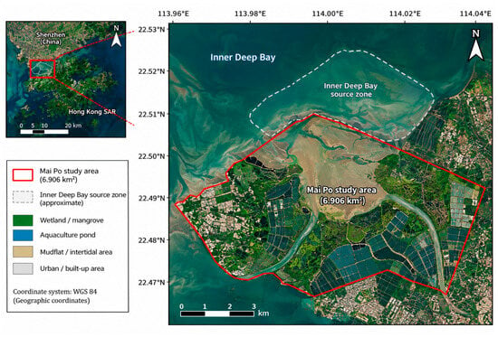
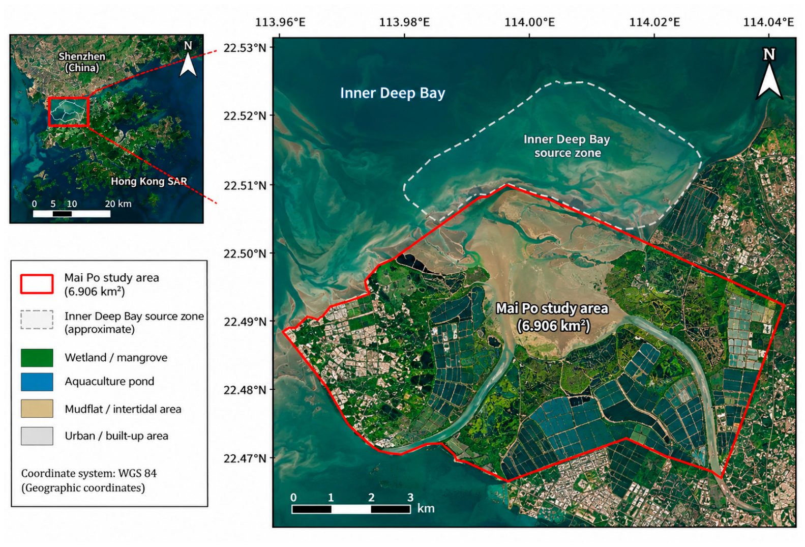
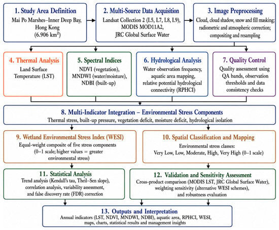
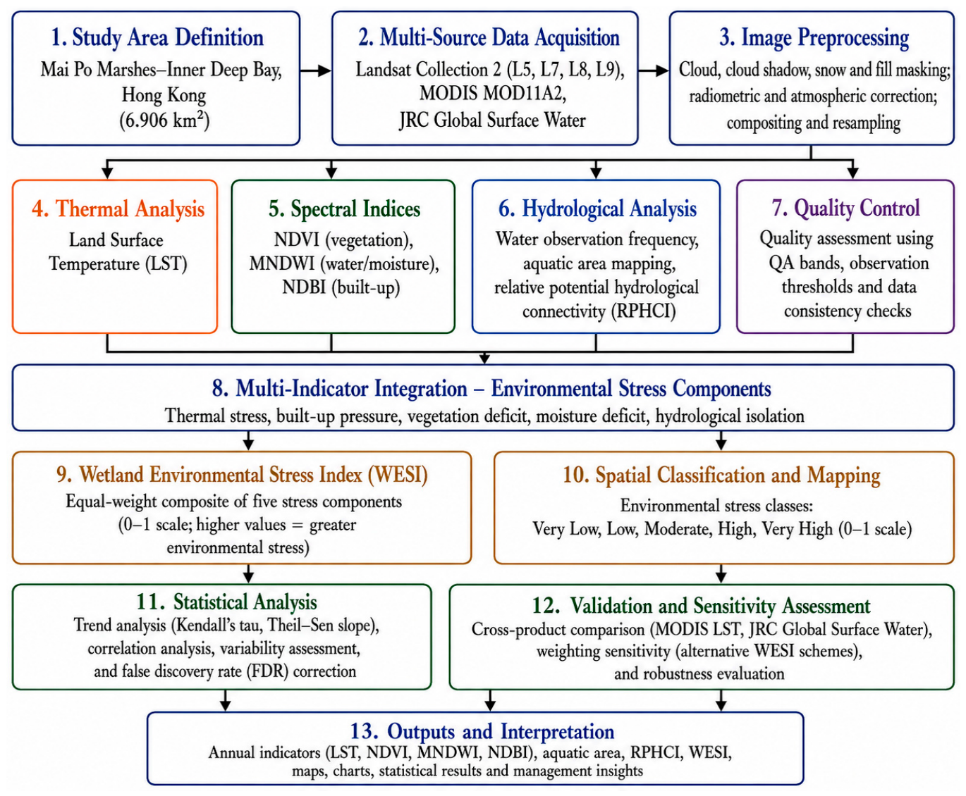
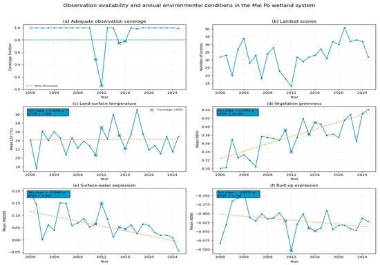
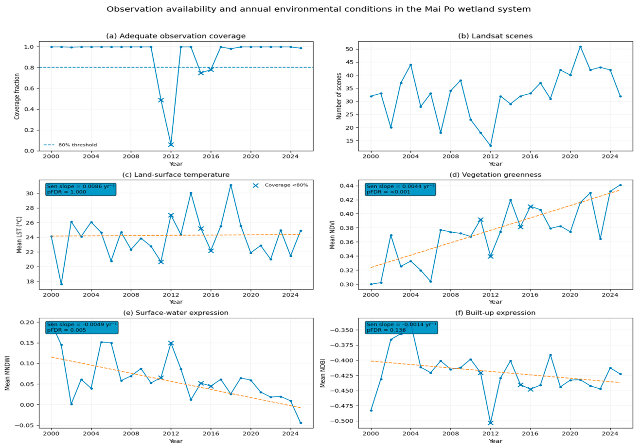
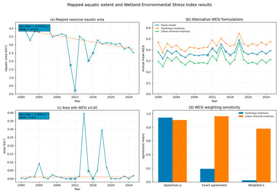
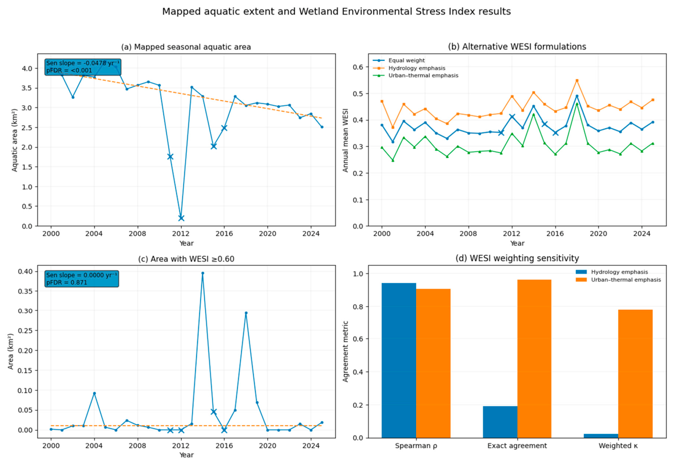
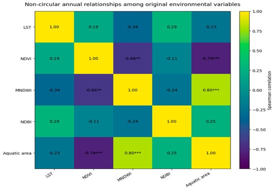
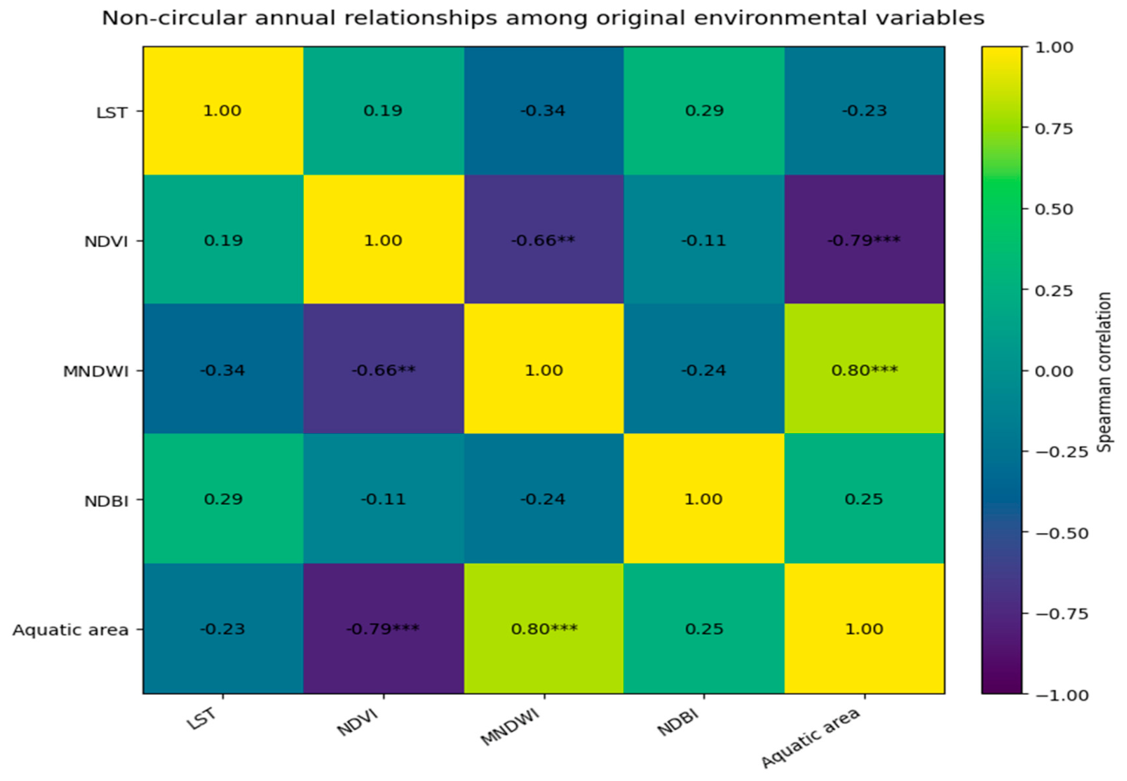

Disclaimer/Publisher’s Note: The statements, opinions and data contained in all publications are solely those of the individual author(s) and contributor(s) and not of MDPI and/or the editor(s). MDPI and/or the editor(s) disclaim responsibility for any injury to people or property resulting from any ideas, methods, instructions or products referred to in the content. |
© 2026 by the authors. Licensee MDPI, Basel, Switzerland. This article is an open access article distributed under the terms and conditions of the Creative Commons Attribution (CC BY) license.