A Python-Based Workflow for Asbestos Roof Mapping and Temporal Monitoring Using Satellite Imagery

Highlights

What are the main findings?

• Python workflow successfully maps asbestos–cement roofs from high-resolution satellite imagery.
• A total of 20–30% pixel threshold optimizes building-level detection.

What are the implications of the main findings?

• The workflow supports scalable, reproducible monitoring of AC roofs.
• Threshold selection should be adapted to the specific objectives of the analysis.

Abstract

The detection and monitoring of asbestos–cement roofing remain a critical public health and environmental challenge, especially in urban and suburban areas where asbestos-containing materials are still widespread due to their extensive use in the 20th century. Although hyperspectral and high-resolution multispectral remote sensing have proven effective for mapping asbestos–cement roofs, many existing approaches rely on proprietary software, limiting transparency, reproducibility, and large-scale adoption. This study presents a fully reproducible, cost-free Python-based workflow for the detection and temporal monitoring of asbestos–cement roofing using high-resolution multispectral WorldView-3 imagery. The workflow integrates atmospheric correction (using the Py6S radiative transfer model), spatial preprocessing, supervised pixel-based classification, postprocessing, and building-level aggregation within an open framework. A Maximum Likelihood Classifier is applied to VNIR and SWIR data using empirically defined roof typologies to enhance class separability. Pixel-level results are aggregated to the building scale through adaptive thresholding enabling the translation of spectral classifications into meaningful building-level information. Tested over the city of Mantua (Italy), the approach achieved reliable classification performance and enabled multi-temporal comparison to identify changes potentially due to roof remediation. Evaluation metrics (precision, recall, and F1-score) highlight the importance of carefully choosing the building-level threshold. By relying exclusively on open-source tools, the workflow enhances transparency, reproducibility, and scalability for long-term monitoring.

1. Introduction

Asbestos-containing materials (ACMs), and in particular asbestos–cement (AC) roofing, remain a major environmental and public health concern in many countries, despite regulatory bans, as their widespread use in building construction throughout the twentieth century has left a persistent legacy in urban environments [1]. Long-term exposure to asbestos fibers is associated with severe respiratory diseases, including asbestosis, lung cancer, and mesothelioma, making the identification and monitoring of AC roofs a priority for global and local authorities [2,3].

Asbestos has been extensively employed in the automotive, construction, manufacturing, power-generation, and chemical industries due to its high tensile strength, non-flammability, and substantial thermal and electrical resistance [4]. Although its adverse effects on public health have been documented since the 1930s [5], the material remains legally permitted in approximately 140 countries. Only around 72 countries [6] have enacted full prohibitions, while major producers such as China, Russia, and Brazil continued mining asbestos well into the current decade [7]. The European Union was among the first to establish regulatory measures, initiating usage restrictions in 1983, which ultimately resulted in a comprehensive ban across all member states [8].

However, such bans do not necessarily imply the complete removal of asbestos-containing structures [9,10]. In many regions, the prohibition solely targets new installations, allowing existing infrastructures to remain in service until the end of their operational lifetime. Consequently, a large number of asbestos-containing structures still require periodic inspection, monitoring, or remediation activities. Such operations expose workers to significant health risks if not properly managed. For this reason, strategies capable of reducing unnecessary on-site inspections are of particular relevance for occupational safety authorities.

In this context, remote sensing-based screening approaches can contribute to minimizing direct exposure of workers to ACMs by supporting preliminary large-scale assessments and by guiding targeted field inspections, an aspect of significant importance for improving worker safety.

Remote sensing techniques such as the use of unmanned aerial vehicles (UAVs) have been increasingly investigated for AC roof mapping at the building scale. Several studies have demonstrated that high-resolution UAV imagery, even when limited to RGB data, can effectively support the identification and quantification of asbestos-containing roofing through visual features, object-based image analysis, or deep learning approaches [11,12,13]. UAV-based surveys allow for very detailed roof-level characterization and can achieve high detection accuracy under controlled acquisition conditions.

However, despite their proven effectiveness at the local scale, UAV-based approaches present inherent limitations when applied to large-area or repeated monitoring tasks. Regulatory constraints, flight permissions, operational costs, and the need for site-specific data acquisition significantly restrict their scalability. Moreover, UAV surveys are often impractical in extensive urban regions or when long-term, multi-temporal monitoring is required. As a result, while UAVs represent a valuable complementary tool for detailed inspections and targeted assessments, satellite-based remote sensing remains more suitable for consistent, large-scale, and repeatable monitoring of asbestos–cement roofing over wide areas.

Over the past two decades, numerous studies have demonstrated the capability of hyperspectral and high-resolution multispectral satellite imagery to discriminate AC materials based on their distinctive spectral response, particularly in the visible and near-infrared regions. Sensors such as MIVIS, APEX, and, more recently, WorldView-3 have been widely used for this purpose, enabling detailed urban-scale mapping [14,15,16,17,18,19,20].

However, many operational asbestos mapping workflows rely on proprietary software environments, which often involve high licensing costs and limited transparency of processing steps. This reliance can limit methodological reproducibility, restrict accessibility for public institutions with limited resources, and complicate the transfer of workflows across different study areas [21]. In the context of environmental monitoring and public health, such limitations contrast with the growing emphasis on open science, reproducible research, and transparent data processing chains.

In addition, the need for temporal monitoring of AC roof removal has become increasingly relevant. While most studies focus on single-date asbestos detection, fewer address multi-temporal analysis aimed at tracking remediation efforts over time [22]. The integration of temporal analysis within a reproducible and scalable workflow remains a key challenge, particularly in complex urban environments.

Recent advances in open-source geospatial libraries and scientific Python ecosystems offer new opportunities to overcome these limitations. Python-based tools for satellite data preprocessing, machine learning, and geospatial analysis now provide capabilities comparable to those of commercial software, while ensuring full transparency, flexibility, and reproducibility of the analytical pipeline [23,24]. Furthermore, the recent proliferation of large-scale open building datasets has provided a robust foundation for urban remote sensing. Platforms such as OpenStreetMap [25], Microsoft Building Footprints [26] and Google Open Buildings [27] offer extensive architectural footprints that can be leveraged to refine roof-level analyses. These resources often include functional attributes (e.g., industrial vs. residential designations, year of construction…) that can serve as critical prior information for material classification, potentially narrowing the search space for AC detection in complex urban environments.

Despite this potential, fully open and end-to-end workflows for AC roof mapping and temporal monitoring are still relatively scarce in the literature.

This study proposes a fully reproducible, Python-based workflow for AC roof mapping and temporal monitoring using high-resolution multispectral satellite imagery. The workflow integrates image preprocessing, supervised classification and postprocessing within an open and transparent processing framework, relying exclusively on freely available Python libraries. The approach is demonstrated through a case study over the city of Mantua (Italy). By enabling scalable and cost-free satellite data processing, the proposed workflow aims to support long-term asbestos monitoring, facilitate data sharing among institutions, and contribute to improved public health protection strategies.

2. Materials and Methods

2.1. Study Area and Data Acquisition

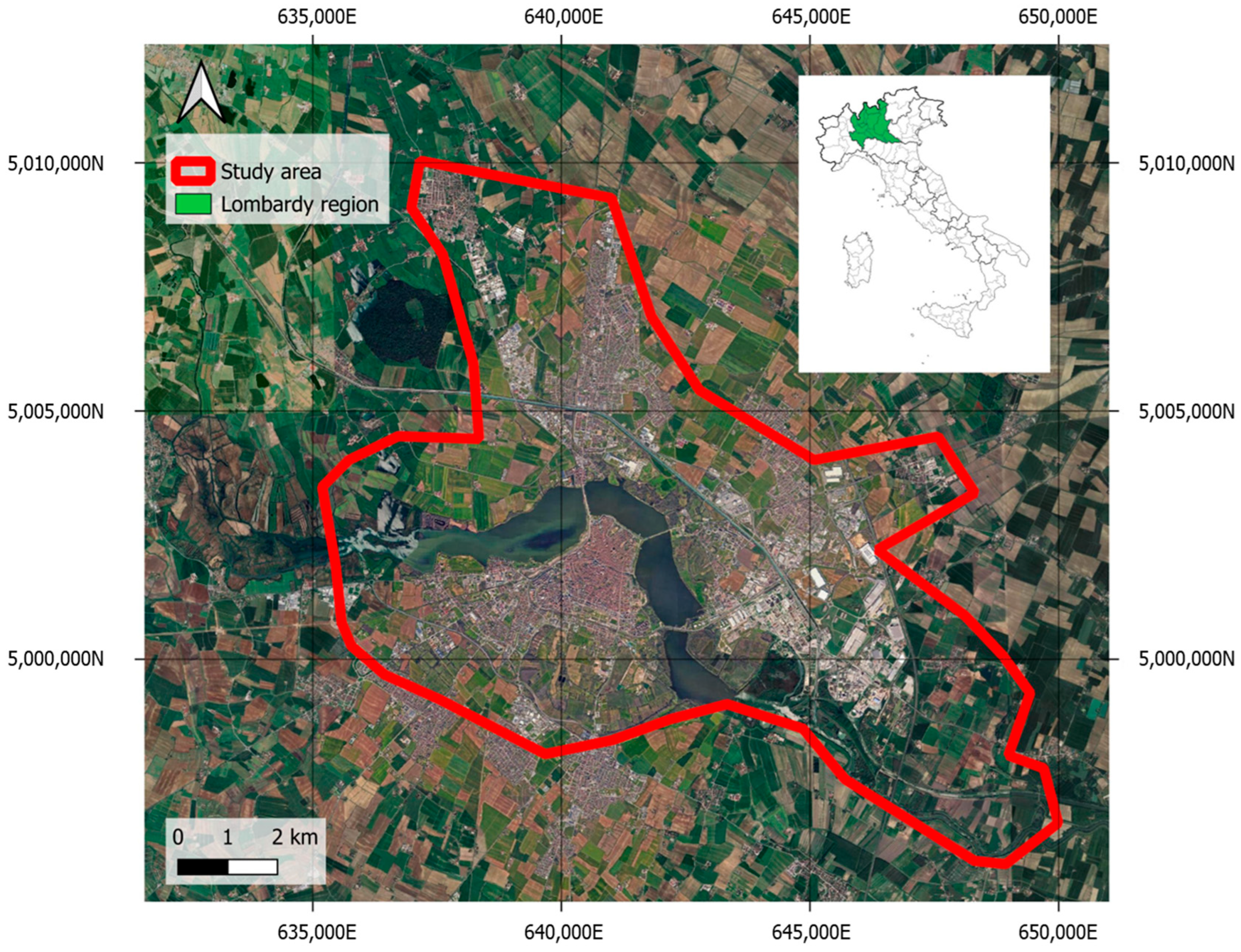
The proposed workflow was tested over the city of Mantua, located in the Lombardy region in northern Italy (Figure 1). Mantua represents a suitable test site for asbestos–cement roof mapping due to its heterogeneous urban structure, which includes historical districts, residential neighborhoods, agricultural surroundings, and a well-developed industrial area.

From a methodological perspective, the city offers an intermediate spatial extent that is well suited for evaluating the transferability of the proposed workflow to urban contexts of different sizes. In addition, part of the industrial area of Mantua is classified as a Superfund Site, reflecting the historical presence of industrial activities associated with asbestos use and reinforcing the relevance of the area for asbestos-related environmental monitoring.

The remote sensing data used in this study consists of high-resolution multispectral imagery acquired by the WorldView-3 satellite in August 2023 and July 2024. The acquisition periods were selected to ensure favorable atmospheric conditions and minimal cloud cover. WorldView-3 provides multispectral data in the visible and near-infrared (VNIR, 8 bands) and shortwave infrared (SWIR, 8 bands) spectral regions, which have been widely recognized as suitable for the detection of AC materials in urban environments [28,29,30].

The spatial resolution of the dataset is consistent with the objectives of roof-scale analysis, with ground sampling distances of 1.24 m/pixel for the VNIR bands and 3.70 m/pixel for the SWIR bands [31].

Ground reference data were collected through field surveys conducted in February 2024, including visual inspections of roofing materials carried out by trained experts. In addition, official remediation records provided by the Mantua Local Health Authority were used to identify buildings that underwent asbestos roof removal or encapsulation between the two acquisition dates. These administrative datasets allowed for independent verification of the temporal changes detected by the proposed workflow, supporting the assessment of AC roof removal and replacement over time.

2.2. Workflow

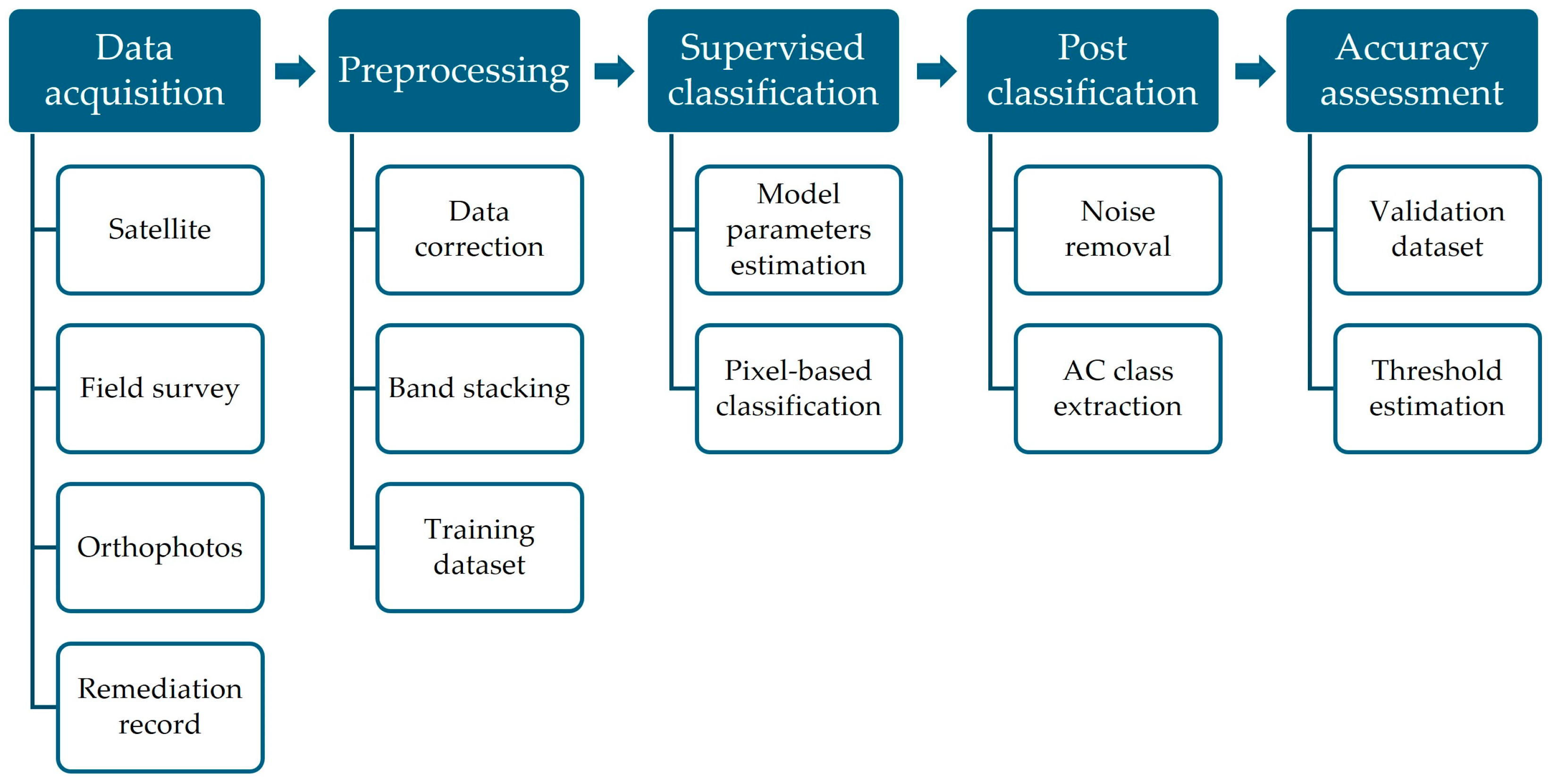
This study proposes an end-to-end, Python-based workflow for AC roof mapping and temporal monitoring using high-resolution multispectral satellite imagery (Figure 2). The workflow is specifically designed for WorldView-3 data, exploiting its spatial and spectral characteristics as well as the sensor metadata provided through accompanying image description files, while maintaining a modular structure that facilitates potential adaptation to comparable high-resolution multispectral datasets.

The workflow integrates multispectral satellite imagery acquired in the visible, near-infrared, and shortwave infrared spectral ranges with a building polygons dataset and ground reference information. Multispectral images represent the primary input, while building polygons are used to spatially constrain the analysis to roof surfaces. Ground reference data are employed both for supervised model training and for independent accuracy assessment.

Processing is organized into a sequence of conceptually independent stages. First, image preprocessing and spectral integration are performed to generate a unified multispectral dataset suitable for roof-scale analysis. The analysis is then restricted to building roofs through the application of a rasterized building mask. Supervised multi-class classification is subsequently applied to discriminate AC roofing from other roof types. The resulting classification map is post-processed to extract the asbestos class and to aggregate pixel-level information at the building scale using area-based criteria.

Classification performance is evaluated through an accuracy assessment focused on the asbestos class, including the analysis of multiple building-level thresholds based on the proportion of pixels classified as asbestos within each roof. Finally, the same workflow is re-applied to multi-temporal imagery acquired at different dates, allowing the assessment of asbestos roof persistence and removal over time. The temporal component of the analysis is supported by updated ground reference information derived from official remediation records.

All processing steps are implemented using open-source Python (v. 3.12.12) libraries. Raster data access and numerical processing are handled through rasterio (v. 1.4.3) [32] and NumPy (v. 2.2.6) [33] libraries, while vector-based spatial operations and building-level analysis rely on GeoPandas (v. 1.1.0) [34]. Statistical modeling and supervised classification are performed using SciPy (v. 1.15.3) [35] and scikit-learn (v. 1.6.1) [24], and image processing routines are supported by scikit-image (v. 0.25.2) [36]. This fully open-source and modular design ensures transparency, reproducibility, and straightforward adaptation to different spatial contexts and multi-temporal analyses.

2.2.1. Preprocessing

All images were preprocessed to ensure spectral and spatial consistency prior to classification. Atmospheric correction was first applied, as it represents a crucial preprocessing step for the reliable exploitation of satellite imagery, particularly when spectral information is used for material discrimination [37].

In this study, atmospheric correction of WorldView-3 images was carried out using the Python interface of the Second Simulation of a Satellite Signal in the Solar Spectrum (6S) radiative transfer model (Py6S, v. 1.9.2)) [38,39]. The 6S model simulates the propagation of solar radiation through the atmosphere by explicitly accounting for molecular scattering, aerosol scattering and absorption, and gaseous absorption processes. Given the sensor geometry, solar geometry, atmospheric conditions, and surface reflectance assumptions, 6S models the radiative components contributing to the at-sensor signal, including the direct surface-reflected radiance, atmospheric path radiance, and multiple scattering effects [40].

Radiometric calibration and geometric metadata required for the correction were extracted from the image description files distributed with the WorldView-3 products. These metadata include sensor viewing geometry, solar geometry, absolute calibration factors, effective bandwidths, and acquisition time, enabling a physically consistent conversion from digital numbers to surface reflectance. Digital numbers were first converted to at-sensor radiance and subsequently to top-of-atmosphere reflectance using band-specific solar exoatmospheric irradiance values provided by the sensor manufacturer [41] (

Table 1. Central wavelength and solar exoatmospheric irradiance values (Esun) for the WorldView-3 spectral bands, as provided by the sensor manufacturer and used for atmospheric correction.

Spectral Band	Central Wavelength (µm)	Esun [W m−2 µm−1] *
Coastal Blue	0.4274	1757.89
Blue	0.4819	2004.61
Green	0.5471	1830.18
Yellow	0.6043	1712.07
Red	0.6601	1535.33
Red Edge	0.7227	1348.08
NIR1	0.8240	1055.94
NIR2	0.9136	858.77
SWIR1	1.2091	479.019
SWIR2	1.5716	263.797
SWIR3	1.6611	225.283
SWIR4	1.7295	197.552
SWIR5	2.1637	90.4178
SWIR6	2.2022	85.0642
SWIR7	2.2593	76.9507
SWIR8	2.3292	68.0988

* Esun is the WorldView-3 band-averaged solar spectral irradiance values for an Earth–Sun distance of 1 AU, normal to the surface being illuminated.

).

Atmospheric correction was then applied on a band-by-band basis using Py6S, accounting for solar zenith angle, sensor viewing angle, acquisition date, and spectral response of each band. Generic atmospheric parameters, representative of the Mantua area, were adopted, including a fixed aerosol optical thickness of 0.15 at 550 nm, which is commonly considered representative of moderate aerosol levels in urban and suburban environments, and a low-altitude assumption consistent with the local topography [42]. The primary objective of this correction was to ensure radiometric consistency across the scene and between different acquisition dates, rather than to retrieve absolute surface reflectance values. Consequently, no in situ atmospheric measurements were required. While variations in atmospheric conditions may influence the corrected values, their impact on classification results is expected to be limited, as the preprocessing prioritizes relative stability for multiband integration. The resulting surface reflectance bands were finally normalized on a per-band basis to a common scale to facilitate subsequent multiband integration and supervised classification.

Following atmospheric correction, individual VNIR and SWIR tiles were mosaicked to produce single-layer rasters for each spectral range. The SWIR raster was then resampled to match the spatial resolution of the VNIR imagery (~1 m) through cubic interpolation, which provides a good compromise between radiometric smoothness and preservation of spectral continuity for classification-oriented analyses. Subsequently, all VNIR and resampled SWIR bands were integrated into a single 16-band raster, creating a unified multispectral image.

Finally, building roof vector data, provided by the Lombardy regional GIS portal [43], were rasterized and applied as a spatial mask to the 16-band image. This operation constrained the analysis exclusively to roof surfaces, reducing computational load and minimizing classification errors associated with non-roof materials, thereby improving the robustness and interpretability of the subsequent asbestos roof mapping.

Training data were defined to represent multiple roof typologies rather than a binary separation between AC and non-AC roofs. This design reflects the statistical assumptions of the Maximum Likelihood Classifier (MLC), which performs optimally when intra-class spectral variability is limited.

Roof surfaces were therefore grouped into a set of empirically defined spectral classes based on their observed spectral signatures. These classes do not correspond to specific roofing materials in a strict semantic sense but represent spectrally homogeneous roof typologies designed to improve class separability for the MLC. The final training classes included water, asbestos–cement, industrial roofs, beige roofs, white roofs, two distinct brown roof typologies, and dark roofs. These classes were selected to capture the main sources of spectral variability observed in the study area and to reduce confusion between AC roofs and other spectrally similar surfaces. Since the ultimate objective of the analysis was the discrimination between AC and non-AC roofs, the individual non-AC roof classes were subsequently aggregated into a single non-AC category during post-classification processing.

To ensure an unbiased evaluation of the classification performance, training and validation datasets were defined using independent sets of building polygons (

Table 2. Number of roofs used for supervised classification training and for independent accuracy assessment.

Class	N° Training Roofs	N° Validation Roofs
AC	15	66
Non AC *	35	66

* The class includes water, industrial roofs, beige roofs, white roofs, two distinct brown roof typologies, and dark roofs.

). Validation samples were selected based on the availability of reliable ground truth data, ensuring both class balance and a spatially distributed coverage of the study area.

2.2.2. Supervised Classification

A supervised pixel-based classification approach was adopted to map AC roofing from the preprocessed multispectral imagery. The MLC was selected, as it has previously demonstrated robust performance for AC roof detection in high-resolution WorldView-3 multispectral imagery [44].

MLC is a parametric classifier that assigns each pixel to the class that maximizes the likelihood of observing its spectral vector, based on class-specific statistical parameters estimated from the training data [45]. It works under the assumption that the spectral signatures of the land cover classes follow a multivariate normal distribution (Equation (1)). For each class, the classifier models the multivariate distribution of spectral values through a mean vector and a covariance matrix, allowing joint exploitation of all available spectral bands [22].

$$g_{i\left(x\right)}=\ln P\left({\omega }_i\right)-{\displaystyle \frac{1}{2}}\ln \left|{\Sigma }_i\right|-{\displaystyle \frac{1}{2}}{\left(x-{\mu }_i\right)}^T{\Sigma }_i^{\left\{-1\right\}}\left(x-{\mu }_i\right)$$

(1)

where $x$ represents the multispectral vector of the pixel being classified, while $P\left({\omega }_i\right)$ denotes the a priori probability of class i. The term $\left|{\Sigma }_i\right|$ refers to the determinant of the covariance matrix for class i, and ${\Sigma }_i^{-1}$ is its inverse, which characterizes the relationships between the different spectral bands. Finally, ${\mu }_i$ represents the mean spectral vector for class i.

This multivariate approach allows the MLC to account for both spectral variability and inter-band correlations, which is essential for discriminating materials with subtle spectral signatures. By incorporating the mean vector and the covariance matrix, the classifier essentially calculates the Mahalanobis distance [46]. Unlike a simple Euclidean distance [47], this metric weighs the spectral distance by the variance and covariance of the class, effectively “shaping” the decision boundary to match the distribution of the training data.

It should be noted that the classification step represents a modular component of the workflow. While an MLC was adopted in this study, alternative machine learning algorithms (e.g., Random Forest or Support Vector Machines) can be readily integrated within the same framework, although this may require adaptation of the training strategy.

All computations were carried out on an Alienware M18 R1 workstation (Dell Inc., Round Rock, TX, USA) workstation featuring a 13th Generation Intel Core i7-13700HX CPU and a 64 GB DDR5 RAM.

2.2.3. Post-Processing

Postprocessing operations were applied to the pixel-based classification results to reduce spatial noise and to aggregate classification outputs at the building level, which represents the final unit of analysis.

Firstly, a median spatial filter with a 3 × 3 kernel was applied to the classified raster to suppress isolated misclassified pixels while preserving roof boundaries. Subsequently, a morphological cleaning step was performed to remove connected components smaller than nine pixels. These small patches are unlikely to represent meaningful roof portions at the spatial resolution of the imagery and were therefore treated as classification noise.

Following noise removal, pixels classified as AC were extracted and converted into point geometries corresponding to pixel centers. These points were spatially intersected with the building polygons to associate each classified AC pixel with its corresponding roof. For each building, the total number of pixels and the number of pixels classified as AC were computed, allowing the estimation of the proportion of AC-covered area per building (ratio between the number of pixels classified as AC and the total number of roof pixels). This indicator enabled the application of threshold-based decision rules, allowing buildings to be flagged as AC-positive when the estimated coverage exceeded a predefined percentage.

2.2.4. Accuracy Assessment

Classification accuracy was evaluated at the building level using an independent validation dataset distinct from the training data. Since the final objective of the workflow is the identification of AC roofs, validation was performed using a binary labeling scheme (AC/non-AC), regardless of the multiclass structure adopted during training.

Ground truth information was primarily derived from field surveys conducted in February 2024, during which roofs were visually inspected and documented. To increase spatial coverage of the validation dataset, field observations were complemented with an interpretation of high-resolution orthophotos [48] acquired before and after the legislative ban on asbestos use [49]. Roofs constructed years after the ban were conservatively labeled as non-AC, under the assumption that ACMs were no longer legally employed.

Building-level predictions were generated by applying increasing thresholds (from 0% to 50%) to the estimated proportion of AC pixels per roof. For each threshold, precision, recall, and F1-score were computed, enabling an objective assessment of the trade-off between false positives and false negatives: precision measures the proportion of correctly identified AC-positive buildings among all buildings classified as AC, recall represents the proportion of correctly identified AC-positive buildings among all reference AC buildings, and the F1-score corresponds to the harmonic mean of precision and recall [50]. This analysis allowed the identification of threshold ranges providing optimal classification performance.

The following equations define the computation of precision (Equation (2)), recall (Equation (3)), and F1-score (Equation (4)). In these expressions, true positives (TP) represent roofs correctly identified as AC-positive, while false positives (FP) denote AC-negative roofs incorrectly classified as AC-positive. Conversely, true negatives (TN) represent AC-negative roofs correctly identified as such, and false negatives (FN) refer to AC-positive roofs misclassified as AC-negative, and n number.

$$Precision={\displaystyle \frac{TP}{TP+FP}}={\displaystyle \frac{nofsuccesfullypredictedasbestosroofs}{nofpredictedasbestosroofs}}$$

(2)

$$Recall={\displaystyle \frac{TP}{TP+FN}}={\displaystyle \frac{nofsuccesfullypredictedasbestosroofs}{nasbestosroofs}}$$

(3)

$$F1=2{\displaystyle \frac{Precision\times Recall}{Precision+Recall}}$$

(4)

2.3. Temporal Monitoring Strategy

Temporal monitoring was implemented by reapplying the same workflow to multispectral WorldView-3 imagery acquired in July 2024. The processing chain, including preprocessing, supervised classification, and postprocessing steps, was kept unchanged to ensure methodological consistency across acquisition dates.

To evaluate the temporal stability of the proposed approach, the training dataset defined for the 2023 acquisition was reused for the classification of the 2024 imagery. This strategy ensures that differences observed between the two dates primarily reflect changes in the image data rather than variations in the training information.

Validation data were instead updated to account for roof remediation activities that occurred between the two acquisition dates, based on official asbestos removal work plans provided by the local health authority. This update allows for a reliable assessment of classification performance in the presence of actual changes in roof materials, while preserving a consistent training strategy across time.

To further investigate the impact of training data consistency, an additional test was conducted by excluding buildings known to have been remediated before the 2024 acquisition from both the training and validation datasets.

3. Results

3.1. Classification Performance and Threshold Analysis

Classification performance was assessed by applying different thresholds to the building-level outputs derived from the 2023 pixel-based classification.

Table 3. Classification performance metrics (precision, recall and f1-score) for thresholds between 0% and 50% of the building area classified as AC.

Threshold	Precision	Recall	F1 Score
0%	0.50	1.00	0.66
10%	0.73	1.00	0.84
20%	0.78	0.97	0.86
30%	0.81	0.92	0.87
40%	0.83	0.86	0.84
50%	0.84	0.82	0.83

reports precision, recall, and F1-score values obtained for thresholds ranging from 0% to 50%. A threshold of 0% corresponds to the absence of any filtering, whereby a building is classified as AC positive if at least one roof pixel is labeled as AC.

At the 0% threshold, recall reached its maximum value (1.00), while precision was substantially lower (0.50), indicating a high number of false positives. Increasing the threshold progressively reduced false detections, resulting in a marked improvement in precision. Thresholds between 20% and 30% produced the highest F1-scores (0.86 and 0.87, respectively), reflecting a balanced trade-off between precision and recall. In the context of asbestos detection, higher recall is prioritized to minimize false negatives (omission errors), ensuring that actual AC roofs are not overlooked. Conversely, a lower precision, resulting from a higher rate of false positives, is considered less critical, as these instances can be subsequently resolved through visual inspection or ground-truthing. The normalized confusion matrices in Figure 3 further illustrate the trade-off between the two thresholds. At 20%, the model achieves very high detection capability for AC roofs (recall = 0.97) but with a higher proportion of false positives (27%). Increasing the threshold to 30% reduces false positives (21%) at the expense of a moderate increase in false negatives (recall = 0.92), confirming a more balanced classification behavior. For higher thresholds (≥40%), precision continued to increase slightly, while recall showed a more pronounced decrease, leading to a reduction in overall F1 performance.

Based on these results, a 30% threshold was selected for the subsequent analyses and comparison between the 2023 and 2024 classifications.

The classification required 7.08 s for ~4.7 million pixels, corresponding to approximately 1.5 µs per pixel. Considering an average roof size of ~900 pixels, this translates to an approximate processing time of ~1.4 ms per roof.

3.2. Building Level AC Mapping Results

The proposed workflow was applied to a total of 25,319 building roof polygons extracted from the regional GIS portal and intersecting the study area. Building-level AC presence was derived from the pixel-based classification by applying decision thresholds to the estimated proportion of AC-covered roof area.

Using a 20% threshold, 2286 buildings were classified as AC, corresponding to approximately 9.0% of the analyzed building stock. When increasing the threshold to 30%, the number of AC-positive buildings decreased to 1554, reflecting a more conservative identification of roofs with higher estimated AC coverage.

Figure 4 illustrates representative examples of the spatial distribution of buildings classified as AC in urban and industrial contexts. The maps highlight the capability of the workflow to identify AC roofs in areas characterized by dense roofing patterns, while preserving spatial coherence.

3.3. Temporal Monitoring Results

Table 4. Comparison of classification performance metrics (precision, recall, and F1-score) and the number of buildings detected as AC roofs for the 2023 and 2024 WorldView-3 acquisitions, using a 30% AC area threshold.

Year	Precision	Recall	F1 Score	N° Buildings
2023	0.81	0.92	0.87	1554
2024	0.79	0.80	0.79	966

summarizes the classification performance obtained for the 2023 and 2024 acquisitions using a 30% AC area threshold. Overall, performance metrics remain comparable across the two years, with a moderate decrease in precision, recall, and F1-score observed in the 2024 results.

A substantial reduction of approximately 37% in the number of buildings detected as AC roofs is observed between 2023 (1554 buildings) and 2024 (966 buildings).

In addition to overall performance metrics, temporal consistency was evaluated using official records of roof remediation activities. Among 80 buildings reported as remediated between the two acquisition dates, 47 were classified as AC roofs in the 2023 results, while 31 remained classified as AC in the 2024 map. Figure 5 provides a visual example of this temporal behavior, showing roofs correctly classified as AC in the pre-remediation image and four of the five remediated roofs no longer detected as AC in the post-remediation acquisition.

The impact of updating the training dataset by excluding remediated buildings was also evaluated for the 2024 classification. The results indicate marginal differences in performance compared to the use of the original 2023 training dataset. For instance, at a 30% threshold, the F1-score remains unchanged (0.79), while at a 20% threshold, it slightly decreases from 0.81 to 0.80.

4. Discussion

4.1. Influence of Thresholding

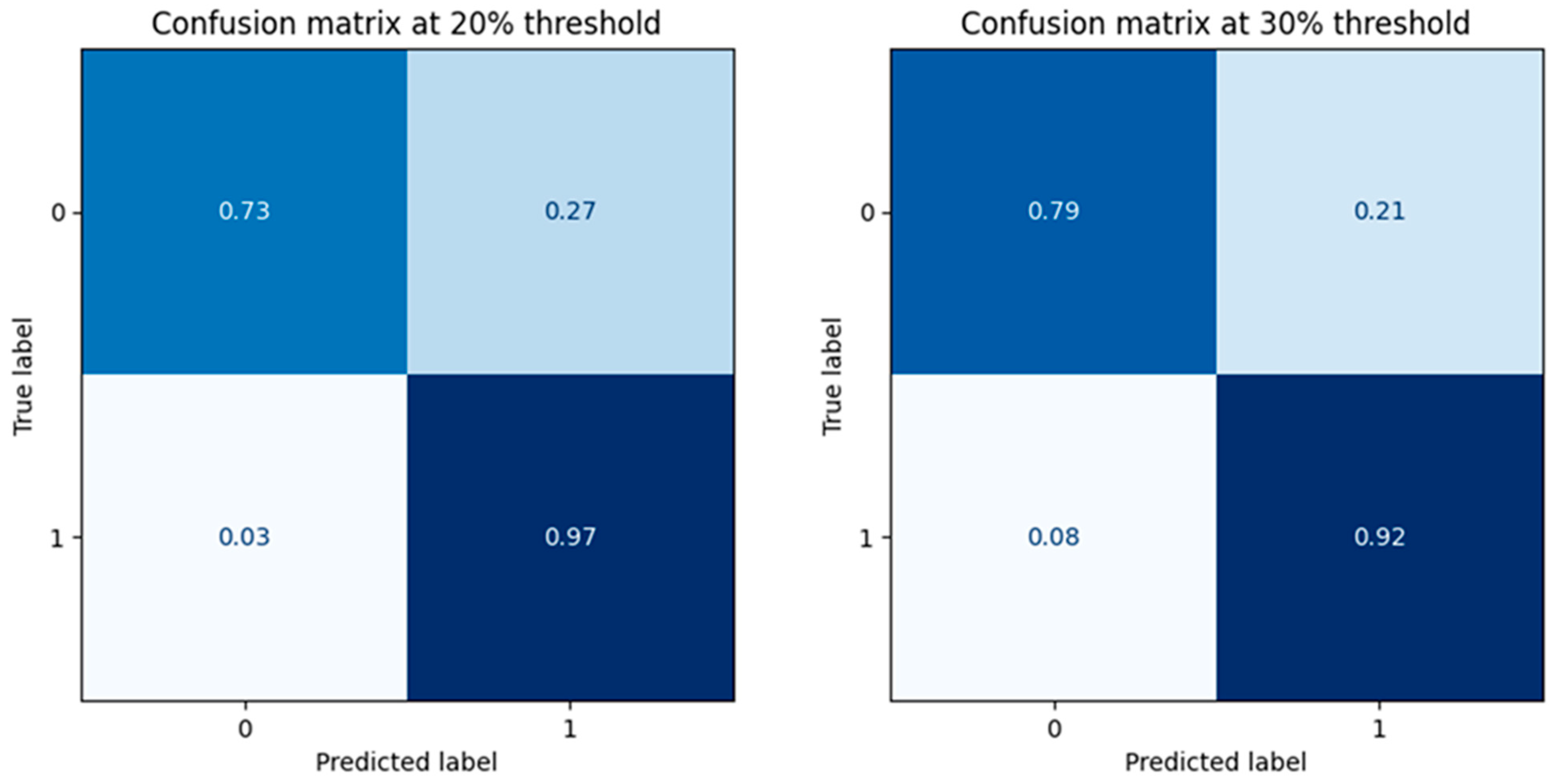
The results demonstrated that threshold selection is a critical parameter in translating pixel-based classification outputs into meaningful building-level information. Low thresholds translate into highly permissive filters, amplifying the effect of isolated misclassified pixels and leading to a substantial number of false positives at the building scale. Conversely, higher thresholds impose a more conservative definition of AC roofs. Although this reduces false positive detections and improves precision, it also increases the omission of AC buildings. The highest F1-scores obtained at intermediate thresholds (20–30%) for the Mantua case study indicate that classification errors are primarily driven by localized pixel-level noise rather than systematic misclassification of entire roofs. This suggests that thresholding plays a decisive role in controlling error propagation from pixels to buildings and should be regarded as an integral part of the classification strategy, as it is not merely a postprocessing step, but a conceptual decision that directly affects the interpretation and usability of AC maps.

Consequently, rather than a fixed parameter, the optimal threshold should be interpreted as a flexible, case-dependent decision rule. While the 20–30% range identified in this study is specific to Mantua, the selection process must be recalibrated when applying the workflow to new contexts. This calibration should account for both the local data characteristics and the specific objectives of the analysis. For instance, thresholds that produce higher recall are preferable in risk-oriented applications, where the priority is to minimize the omission of potentially hazardous AC roofs, even at the expense of an increased number of false positives. This approach is common in healthcare applications of machine learning, where maximizing the True Positive is more important than having better overall accuracy [51]. Conversely, thresholds associated with higher precision are more appropriate when the aim is to ensure that buildings classified as AC are truly affected. The F1-score helps identify thresholds that achieve a balanced trade-off between precision and recall.

4.2. Impact of Building Vector Data Quality

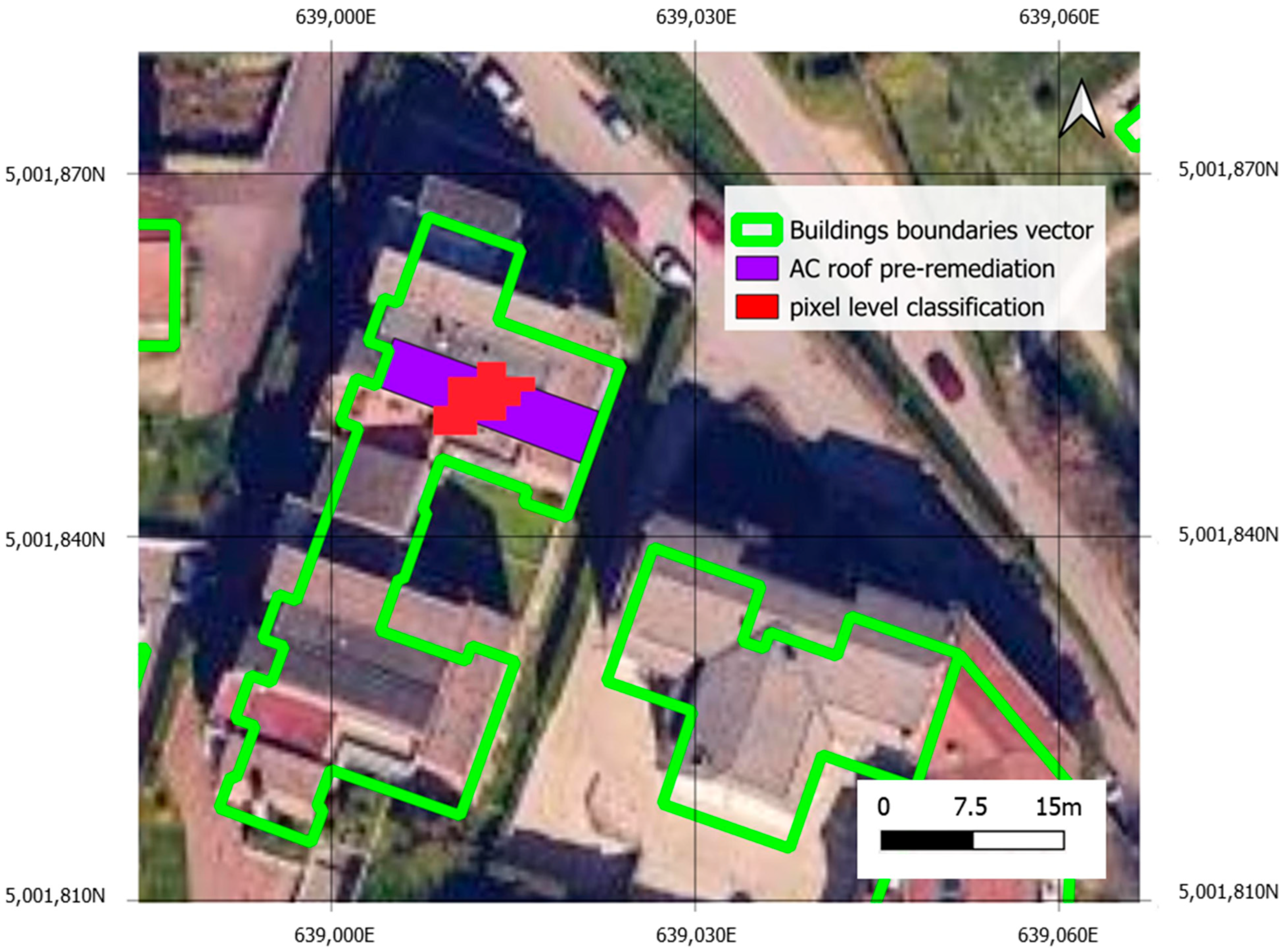
The results also show that the accuracy of the classification is not only influenced by the chosen threshold, but also by the quality and geometric accuracy of the building vector data used for masking and aggregation. Misalignments between roof outlines and actual roof extents may lead to incorrect estimation of the proportion of AC classified pixels and, consequently, to incorrect final labeling. 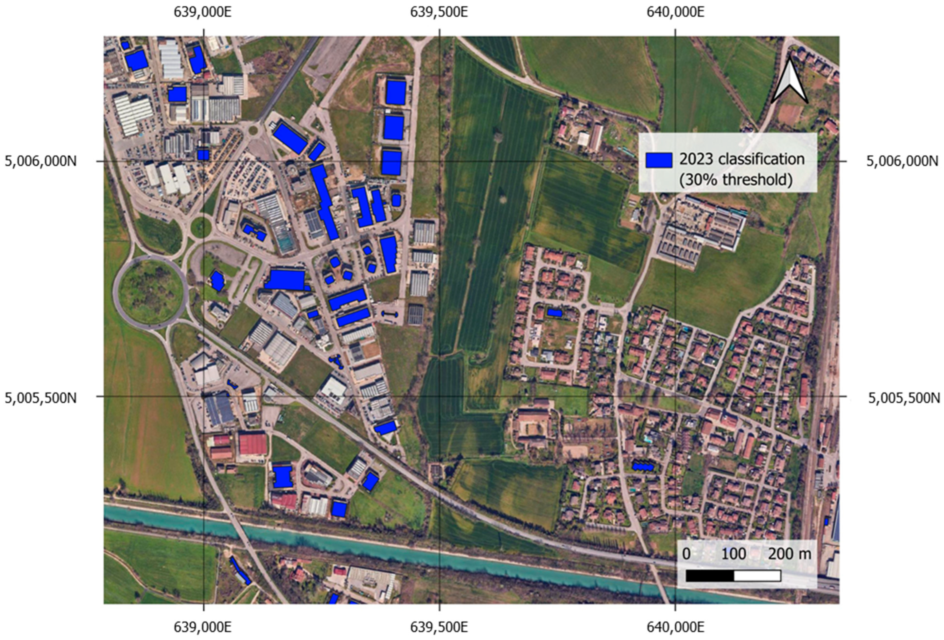Figure 6 illustrates a representative example in which a single building polygon aggregates multiple adjacent roof units. Although the pixel-based classification correctly identifies AC on one of the individual roofs, the proportion of AC-classified pixels remains below the minimum threshold when computed over the entire polygon area. As a result, the building is not labeled as AC at any of the tested thresholds, despite the presence of asbestos.

More broadly, this interaction between spectral classification and vector geometry shapes the workflow’s error profile. FP detections are primarily associated with roofing materials that exhibit spectral responses similar to AC, such as industrial or weathered surfaces, and with residual pixel-level noise. Conversely, FN, which are more critical in the context of public health monitoring, are mainly driven by two factors: geometric inaccuracies or aggregation effects in building polygons, which dilute the contribution of correctly classified pixels; the presence of mixed pixels at roof boundaries.

To mitigate these errors, several targeted strategies can be integrated into the workflow. To address edge effects and mixed pixels, the application of a negative buffer (inward erosion) to building polygons prior to pixel extraction would reduce edge-related classification errors. Furthermore, improving building segmentation to treat individual roof units as separate entities would minimize the dilution effect.

4.3. Temporal Consistency of the Workflow

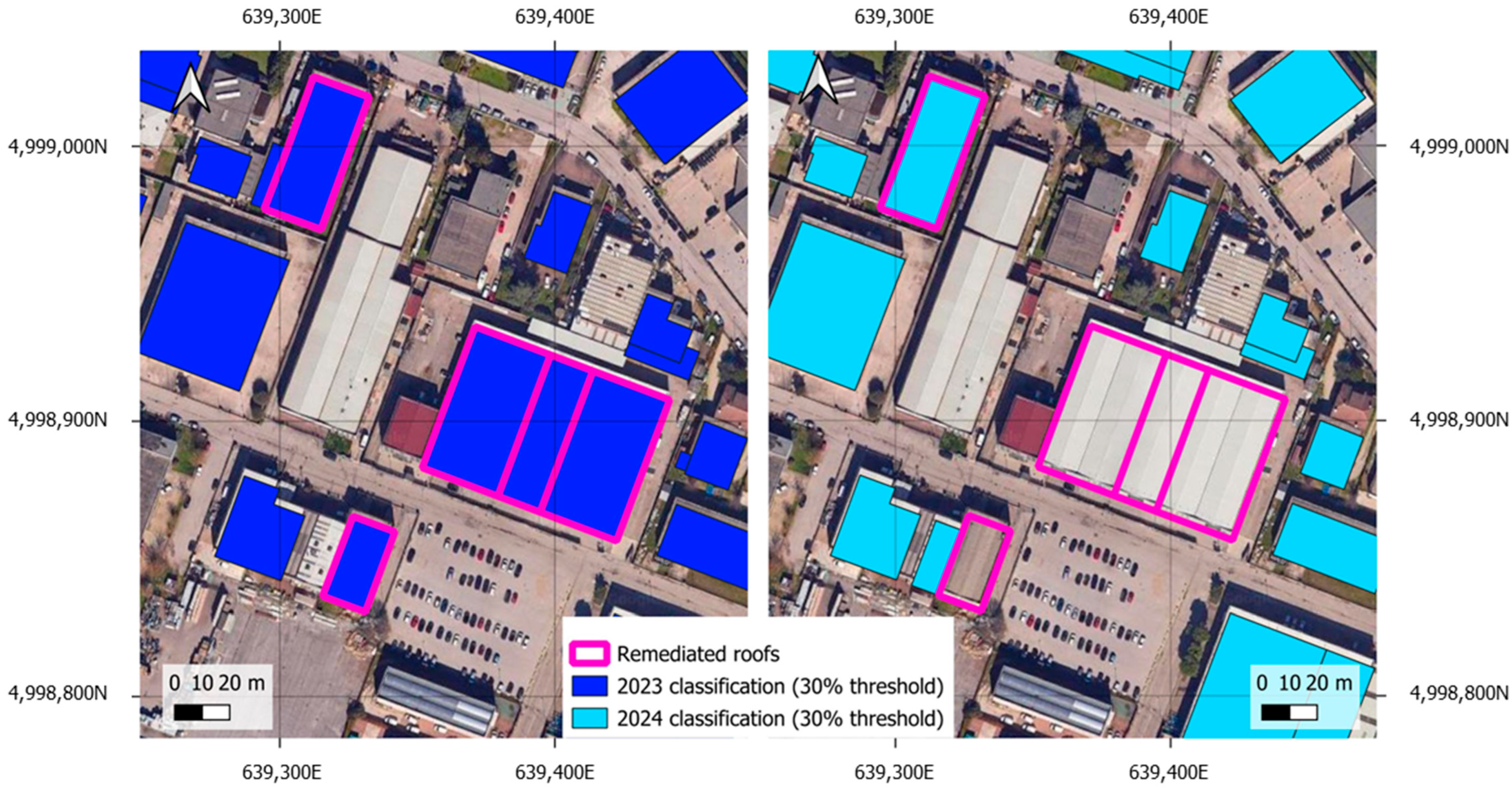
The application of an unchanged workflow to multi-date WorldView-3 imagery indicates a generally consistent classification performance over time, as reflected by comparable precision, recall, and F1-score values across the two acquisitions. At the same time, a marked reduction in the number of buildings classified as AC was observed between 2023 and 2024, a difference that cannot be attributed solely to documented remediation activities. Part of this reduction is explained by the correct exclusion of several remediated roofs that were identified as AC in the 2023 classification and no longer detected in the 2024 results. However, not all remediated buildings were accurately identified, and the remaining inconsistencies are likely due to variations in image acquisition conditions and differences in roof spectral responses. To better quantify this uncertainty, the observed reduction of 588 buildings (in the 30% threshold classification) was compared with official remediation records. Among the buildings reported as remediated (133), the classification correctly identified 46.6% (62 out of 133) of the removals. The remaining 455 buildings that were not identified in 2024 (29.2% of the 1554 detected in 2023) can thus be attributed to classification variability and other data-related factors. Incorporating additional training data representing a wider range of conditions is expected to improve the model’s robustness to these effects.

An additional source of uncertainty comes from the decision to keep the training dataset unchanged across acquisition dates. Although this choice ensured methodological consistency, it also introduced potential inaccuracies, as some buildings labeled as AC in the 2023 training data had been remediated before the 2024 acquisition. This mismatch between training labels and actual roof conditions may have contributed to the observed differences in classification outcomes, highlighting a key limitation when applying supervised classifiers for long-term monitoring without periodic updating of training data.

The additional test performed by excluding remediated buildings from the training dataset provides further insight into this limitation. While this approach improves the temporal consistency of the ground truth, it does not result in a meaningful increase in classification performance, with F1-scores remaining essentially unchanged across the evaluated thresholds. While the impact on performance is limited in the short term, this strategy may become less effective over longer monitoring periods, as the mismatch between training data and real conditions progressively increases. From an operational perspective, this suggests that maintaining a reliable multi-temporal dataset requires not only the removal of outdated samples, but also the integration of updated data to compensate for the resulting loss of spectral information that might affect the classification.

4.4. Practical Considerations and Perspectives

The proposed workflow is designed to support operational AC roof mapping using satellite data and open-source tools. Its performance is influenced by several practical factors that should be considered when transferring the methodology to other study areas.

Firstly, it should be emphasized that the effectiveness of the proposed methodology is strongly influenced by the spatial and spectral characteristics of the input imagery. In particular, the very high spatial resolution provided by sensors such as WorldView-3 represents a key factor for enabling roof-level analysis. While the workflow is designed in a modular and sensor-agnostic manner, its transferability to other multispectral sensors depends on the availability of comparable spatial resolution and suitable spectral bands for material discrimination. The use of lower-resolution imagery may limit the ability to accurately identify AC surfaces, especially in dense urban contexts or for small and heterogeneous roof structures. In addition, the applicability of the workflow relies on the availability of the metadata required for atmospheric correction, which is necessary to ensure radiometric consistency across acquisitions.

The quality and geometric accuracy of building vector data play an important role in building-level final classification. When vector data does not accurately match individual roof units, the proportion of pixels classified as AC may be underestimated or overestimated. Using updated and well-segmented building datasets is therefore recommended whenever available.

Another practical aspect concerns training data. In this study, a single training dataset was intentionally reused for multi-temporal analysis to ensure methodological consistency across acquisition dates. While this strategy enables direct temporal comparison, the results highlight the need for periodic updating or incremental expansion of training samples, particularly in areas undergoing remediation activities, to maintain classification reliability over time In this context, future developments could adopt an iterative updating strategy, in which classification results from previous acquisitions are used to support the identification of reliable new training samples, combined with external information (e.g., remediation records or visual interpretation) which can also support the validation of newly identified samples prior to their inclusion in the training dataset, as well as the following remediation operations. This approach would enable progressive refinement of the training dataset, improving its representativeness and temporal consistency over extended monitoring periods.

The results obtained through the proposed workflow should be interpreted within the framework of a screening-oriented approach. The presence of both false positives and false negatives implies that building-level classifications cannot be used as direct evidence for enforcement actions. False positives lead to a conservative overestimation of asbestos presence and do not represent a critical issue from a public health perspective, whereas false negatives require particular attention, as they may temporarily delay the identification of existing AC roofs.

For this reason, output generated through the proposed methodology should be managed exclusively by competent public authorities and specialized professionals. These data are intended to support territorial-scale assessments of the overall extent of AC roofing and to guide the prioritization of on-site inspections, while detailed field verification by local control bodies remains indispensable before initiating legal or administrative measures, such as mandatory removal orders.

Despite these considerations, the overall stability of the results across two acquisition dates indicates that the workflow provides a reliable basis for large-area and repeated monitoring. Future developments may focus on the integration of longer multi-temporal image series and on strategies to progressively reduce the dependence on manually defined training data, for example, through incremental updating or semi-automatic sample selection based on stable spectral patterns.

5. Conclusions

This study presents a fully reproducible and cost-free workflow for the detection and temporal monitoring of asbestos–cement roofing using multispectral WorldView-3 imagery and open-source Python libraries. The proposed approach demonstrates that reliable building-level AC mapping can be achieved without reliance on proprietary software, thereby lowering economic and technical barriers that often limit the operational use of remote sensing for environmental health applications.

The results confirm that a transparent pixel-based supervised classification framework, combined with a building-level aggregation strategy, provides robust and interpretable outputs for urban-scale asbestos monitoring. In particular, the analysis highlights the central role of threshold selection in translating pixel-level classifications into meaningful building-level indicators, showing that this step represents a key methodological decision rather than a simple postprocessing operation.

The application of the same workflow to multi-date imagery further demonstrates its suitability for temporal monitoring, enabling consistent assessment of changes in AC roof presence over time. Although variations in acquisition conditions and ground truth availability can influence the results, the overall stability of performance supports the use of the proposed methodology for repeated monitoring scenarios.

When applied with due caution, the proposed open-source methodology offers significant economic and occupational safety advantages. Repeated monitoring over time allows progressive refinement of the information base, improving data reliability and enabling a substantial reduction in unnecessary field inspections. This translates into lower operational costs and, more importantly, into reduced direct exposure of workers to ACMs.

By relying exclusively on open-source tools and reproducible procedures, the workflow represents a cost-effective and safer support tool for public administrations, optimizing resource distribution, improving worker protection, and enhancing long-term asbestos management strategies, provided that data sharing remains controlled and aligned with institutional responsibilities.