Optimized Hybrid Deep Learning Framework for Reliable Multi-Horizon Photovoltaic Power Forecasting in Smart Grids

Abstract

Accurate short-term forecasting of photovoltaic (PV) output is critical to managing the variability of PV generation and ensuring reliable grid operation with high renewable integration. We propose an enhanced hybrid deep learning framework that combines Temporal Convolutional Networks (TCNs), Gated Recurrent Units (GRUs), and Random Forests (RFs) in an optimized weighted ensemble strategy. This approach leverages the complementary strengths of each component: TCNs capture long-range temporal dependencies via dilated causal convolutions; GRUs model sequential weather-driven dynamics; and RFs enhance robustness to outliers and nonlinear relationships. The model was evaluated on high-resolution operational data from the Yulara solar plant in Australia, forecasting horizons from 5 min to 1 h. Results show that the TCN-GRU-RF model consistently outperforms conventional benchmarks, achieving R² = 0.9807 (MAE = 0.0136; RMSE = 0.0300) at 5 min and R² = 0.9047 (RMSE = 0.0652) at 1 h horizons. Notably, the degradation in R² across forecasting horizons was limited to 7.7%, significantly lower than the typical 10–15% range observed in the literature, highlighting the model’s scalability and resilience. These validated results indicate that the proposed approach provides a robust, scalable forecasting solution that enhances grid reliability and supports the integration of distributed renewable energy sources.

1. Introduction

Global energy demand has been rising steadily at an average rate of 2.3% per year since 2010, while fossil fuels remain the dominant source of carbon dioxide emissions, contributing approximately 86% of global totals. This dual challenge underscores the urgent need for a rapid transition to renewable energy systems [1,2]. Among these, PV technology has emerged as a leading low-carbon solution, driven by rapidly declining costs and its suitability for large-scale deployment. According to IRENA (International Renewable Energy Agency) (2025), global installed PV capacity reached 1865 GW by the end of 2024, accounting for 42% of total renewable capacity, with 452 GW added in 2024 alone representing a 32.2% year-on-year increase [3]. This growth highlights the increasing competitiveness of solar energy against fossil fuels, enabled by supportive policies and reinforced by climate imperatives. However, the rapid integration of PV into modern power systems presents operational and economic challenges due to its inherent variability and intermittency. Crucially, PV generation is highly sensitive to weather fluctuations, which must be balanced against the continuous and predictable nature of electricity demand. Consequently, accurate short-term forecasting of PV output is essential for grid operators and energy market participants to maintain system stability, optimize operations, and ensure efficient market participation [4,5,6]. Reliable forecasting also facilitates the economic integration of solar energy into electricity markets by improving trading strategies [7,8].

Furthermore, PV forecasting methodologies have undergone significant advancements. Early efforts relied on physical models, which employed panel characteristics and meteorological variables such as irradiance and temperature to generate physically interpretable forecasts. Although accurate under well-defined conditions, these models were often complex and lacked adaptability to dynamic environments [9,10]. Statistical methods such as ARMA and ARIMA provided improvements by capturing temporal correlations but were limited in handling nonlinear dynamics and rapid fluctuations [11]. The advent of machine learning (ML) introduced powerful data-driven alternatives capable of modeling nonlinearities without explicit physical assumptions. Comprehensive reviews of probabilistic forecasting [12] indicate that while statistical methods offer interpretability, machine learning approaches demonstrate superior capability in capturing the non-linear stochastic volatility inherent in renewable energy generation. Algorithms such as Support Vector Machines (SVM), k-Nearest Neighbors (kNN), and RF demonstrated strong predictive ability, particularly with large heterogeneous datasets [13,14]. RFs, in particular, have shown robustness to overfitting and strong performance in handling diverse feature types [15,16]. More recently, deep learning (DL) has transformed PV forecasting by enabling advanced modeling of temporal dependencies and spatial patterns in solar data [17,18]. For instance, recent studies have successfully applied deep learning architectures to handle complex environmental data: [19] utilized multi-source information fusion for high-precision PV identification, while [20] integrated deep learning with GIS to accurately assess solar potential in dense urban environments. These works highlight the capacity of deep neural networks to extract intricate features from heterogeneous data sources. Recurrent Neural Networks (RNNs), notably Long Short-Term Memory (LSTM) and GRU architectures, have excelled in time-series forecasting, with LSTMs overcoming the vanishing gradient problem and GRUs offering comparable performance with reduced computational cost [21,22,23,24]. Convolutional Neural Networks (CNNs), originally developed for image processing, have been adapted into TCNs, which exploit dilated causal convolutions to capture long-range dependencies efficiently, making them highly effective for multi-scale temporal feature extraction [25,26,27].

Despite these advances, no single algorithm has demonstrated universal superiority across all temporal horizons, weather conditions, and geographic contexts [28]. This limitation has motivated the development of hybrid models, which integrate complementary approaches to exploit their respective strengths [29,30]. Recent work confirms that hybrid architectures often outperform standalone models. For instance, CNN-LSTM hybrids combine spatial feature extraction with temporal sequence learning [31,32] attention-based architectures enhance dynamic feature weighting [33,34,35], and TCN-GRU hybrids integrate hierarchical feature extraction with long-term dependency modeling [36,37,38]. Additional contributions include BiLSTM-CNN for multi-step forecasting [39], GRU-SVM hybrids for combining sequential learning with margin-based classification [40], and decomposition-driven hybrids addressing data complexity [41,42,43]. Collectively, these studies demonstrate that hybridization often succeeds where single models fail. A critical review of the existing literature reveals that current photovoltaic (PV) power forecasting methods utilize methodologies that exhibit several limitations. First, no single model demonstrates consistent performance across all forecast horizons, resulting in notable accuracy degradation when transitioning from very short-term horizons (e.g., 5 min) to longer horizons (e.g., 1 h). Second, most approaches struggle to simultaneously capture multi-scale temporal dependencies and rapid sequential fluctuations induced by meteorological variability, both of which are critical for reliable forecasting. Third, real-world solar power plant data are often affected by non-linearities, noise, missing values, or outliers, which can significantly degrade the performance of deep learning models. Finally, many existing hybrid models employ naive or uniform fusion mechanisms (such as simple averaging) that fail to differentiate between component models based on their predictive reliability, thereby limiting their overall accuracy and robustness.

To address these challenges, this study proposes a novel hybrid architecture combining a TCN, GRU, and RF. The TCN-GRU-RF model leverages the complementary strengths of its components: the TCN captures hierarchical temporal dependencies, the GRU models long-term sequential dynamics under variable meteorological conditions, and the RF enhances robustness to non-linearities and heterogeneous data. An optimized fusion mechanism calibrates the contribution of each component based on its predictive reliability (inverse RMSE), ensuring accurate and stable forecasts across diverse conditions while maintaining computational efficiency. The main contributions of this work are summarized as follows:

(1)

This study proposes an enhanced hybrid forecasting framework that integrates a TCN, a GRU, and a RF within an optimized weighted fusion strategy. By leveraging the complementary strengths of these components, the framework effectively captures hierarchical temporal dependencies, models rapid sequential fluctuations, and enhances robustness against outliers and data irregularities. The optimized weighting mechanism calibrates the contribution of each model according to predictive reliability, thereby improving the overall stability and accuracy of short-term PV power forecasts compared to individual models or hybrid models with uniform or naive fusion schemes.

(2)

Through extensive comparative experiments and ablation analyses, this study systematically evaluates the performance of the proposed model across multiple forecasting horizons (5, 15, 30, and 60 min) and under diverse meteorological conditions. The results confirm that the TCN-GRU-RF hybrid consistently outperforms benchmark approaches such as LSTM, CNN, RF, and CNN-GRU, achieving an R² of 0.9807 for 5 min forecasts and 0.9047 for 1 h forecasts, maintaining only a 7.7% reduction in R² across horizons, significantly lower than typical declines in existing models, and demonstrating its robustness, scalability, and adaptability under diverse weather conditions.

(3)

A large-scale validation is conducted using more than 210,000 five-minute observations collected over two years. The TCN is responsible for extracting multi-scale temporal features, the GRU effectively models short-term variability, and the RF enhances resilience against anomalies in the data. The results highlight its operational value for grid operators, as it provides reliable short-term forecasts that can mitigate the intermittency of solar generation, strengthen system stability, and facilitate the integration of renewable energy into electricity markets.

The rest of this paper is organized as follows. Section 2 presents the methodological foundations, including a description of the TCN, GRU, and RF models and their integration. Section 3 describes the experimental design, dataset preparation, and performance evaluation. Section 4 concludes with the main findings and outlines future research directions.

2. Materials and Methods

This section presents the methodological framework of the proposed TCN-GRU-RF model. The architecture integrates the complementary strengths of TCNs, GRUs, and RFs through an optimized fusion mechanism. An overview of the framework, including data preprocessing, individual model training, and the ensemble fusion process, is illustrated in Figure 1. As shown in Figure 1, the framework consists of three main stages: (1) data acquisition and preprocessing, (2) individual model development (TCN, GRU, and RF), (3) optimized fusion for generating the final forecasts, (4) and results analysis.

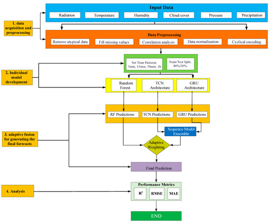
Figure 1. Proposed model framework.

2.1. Data Acquisition and Preprocessing

2.1.1. Data Description

The experimental dataset was obtained from the Yulara PV Power Plant in Uluru, Australia (25.24° S, 131.04° E) [41]. It consists of 210,240 samples recorded at a 5 min resolution (288 observations per day) over a two-year period from January 2021 to December 2022. The dataset includes photovoltaic (PV) power generation alongside key meteorological variables: global horizontal irradiance (GHI), ambient temperature, wind speed, and relative humidity. To address the absence of certain atmospheric variables (e.g., cloud cover and specific humidity), supplementary hourly meteorological data were sourced from OpenWeatherMap [42].

These data were temporally aligned with the primary dataset by resampling to 5 min intervals using a combination of linear and spline interpolation. This integration produced a high-resolution, multi-variable dataset that captures both solar and meteorological dynamics, providing a reliable foundation for modeling the influence of weather variability on PV power output.

2.1.2. Missing Data Imputation and Cleaning

Missing or corrupted values, primarily caused by sensor or communication errors, were corrected using linear temporal interpolation. Specifically, a missing value at time t was estimated as follows:

$$x_t=x_{t_1}+{\displaystyle \frac{t-t_1}{t_2-t_1}}\times (x_{t_2}-x_{t_1})$$

(1)

where $x_t$ is the imputed value at time t; $x_{t_1}$ and $x_{t_2}$ are the known values immediately before and after t, respectively; and $t_1$ and $t_2$ denote the nearest valid timestamps surrounding t. This method preserves continuity between known data points while minimizing the risk of introducing artificial fluctuations. During nighttime periods, PV power output was explicitly set to zero. This preprocessing step is physically justified as solar irradiance is zero at night; forcing these values eliminates sensor noise and prevents the model from learning irrelevant fluctuations during non-productive hours. Outliers, such as negative active power readings or irradiance values below zero, were identified and clipped to physically plausible ranges using quantile-based thresholds, thereby ensuring the integrity and reliability of the dataset.

2.1.3. Features Scaling and Cyclical Encoding

All input features were normalized to [0, 1] using Min–Max scaling:

$$x_t^{\prime }={\displaystyle \frac{x_t-x_{min}}{x_{max}-x_{min}}}$$

(2)

where $x_t$ is the original value at time t; $x_{\min }$ and $x_{\max }$ are the minimum and maximum values of the feature, respectively; and $x_t^{\prime }$ is the normalized value. Importantly, these scaling parameters were computed exclusively from the training dataset to prevent data leakage and ensure unbiased model evaluation.

To represent temporal cyclicality, hour-of-day and month-of-year were encoded via sine/cosine transformations:

$${\mathrm{hour}}_{\mathrm{s}\mathrm{i}\mathrm{n}}=\mathrm{s}\mathrm{i}\mathrm{n}\left(2\pi {\displaystyle \frac{\mathrm{hour}}{24}}\right),{\mathrm{hour}}_{\mathrm{c}\mathrm{o}\mathrm{s}}=\mathrm{c}\mathrm{o}\mathrm{s}\left(2\pi {\displaystyle \frac{\mathrm{hour}}{24}}\right)$$

(3)

$${\mathrm{month}}_{\mathrm{s}\mathrm{i}\mathrm{n}}=\sin \left(2\pi {\displaystyle \frac{\mathrm{month}}{12}}\right),{\mathrm{month}}_{\mathrm{c}\mathrm{o}\mathrm{s}}=\mathrm{c}\mathrm{o}\mathrm{s}\left(2\pi {\displaystyle \frac{\mathrm{month}}{12}}\right)$$

(4)

This preserves daily/seasonal periodicity, enabling better diurnal/seasonal pattern capture.

2.2. Model Architectures

2.2.1. Temporal Convolutional Network (TCN)

TCNs adapt Convolutional Neural Networks for sequence modeling, incorporating causal convolutions, dilated convolutions, and residual connections to process time-series data while preserving temporal causality as shown in Figure 2.

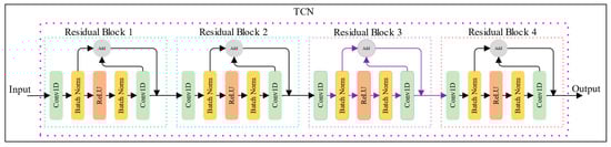
Figure 2. Schematic architecture of the Temporal Convolutional Network (TCN).

Causal convolutions ensure predictions at time t depend only on inputs from t and prior variables:

$$F(s)=(x{\ast }_{d}f)(s)={\displaystyle {\sum }_{i=0}^{k-1}} f(i)\cdot x_{s-d\cdot i}$$

(5)

where $F\left(s\right)$ is the output value at sequence position s; $x$ is the input sequence; $f$ represents the filter of length $k$; $d$ is the dilation factor; and $s-d\cdot i$ ensures causality by referencing only current and previous time steps.

Dilated convolutions exponentially expand receptive fields with network depth (d = 2ⁱ for layer i). An N-layer TCN’s effective receptive field r is as follows:

$$r=1+(k-1){\displaystyle {\sum }_{i=0}^{N-1}} d_i=1+(k-1)(2^N-1)$$

(6)

where r is the size of the effective receptive field (number of input time steps considered); k the filter size; N the number of layers in the TCN; and d_i is the dilation factor for layer i.

TCNs excel in solar forecasting by capturing multi-scale temporal patterns influencing PV output [44].

Residual connections, as illustrated in Figure 2, facilitate gradient flow through deep networks and mitigate the vanishing gradient problem. A typical TCN residual block comprises two dilated causal convolutional layers, each followed by weight normalization, ReLU activation, and dropout regularization. The residual connection is formulated as follows:

$$o=\mathrm{ReLU}(x+F(x\left)\right)$$

(7)

where o represents the final output of the block; $F\left(x\right)$ the output of the convolutional operations; and $x$ is the input to the residual block.

2.2.2. Gated Recurrent Unit (GRU)

GRUs (Figure 3) address vanishing gradients while offering greater computational efficiency than LSTMs. GRU operations at time t are as follows:

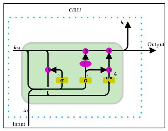
Figure 3. Schematic diagram of the Gated Recurrent Unit (GRU).

• Update Gate (retains historical information):

$$z_t=\sigma \left(W_z\cdot [h_{t-1},x_t]+b_z\right)$$

(8)

The update gate $z_t$ decides how much of the past memory $h_{t-1}$ should be carried forward to the future. A value of 1 means “keep everything,” and 0 means “forget everything.”

• Reset Gate (modulates past information influence):

$$r_t=\sigma \left(W_r\cdot [h_{t-1},x_t]+b_r\right)$$

(9)

The reset gate $r_t$ decides how much of the past memory is relevant for computing a new candidate state. It allows the model to “reset” or ignore parts of the past that are no longer useful.

• Candidate Hidden State:

$${\tilde{h}}_t=\mathrm{t}\mathrm{a}\mathrm{n}\mathrm{h}\left(W\cdot [r_t\odot h_{t-1},x_t]+b\right)$$

(10)

This creates a “proposal” for the new hidden state, based on the current input $x_t$ and the gated previous state $r_t\odot h_{t-1}$. The reset gate controls how much of the past influences this proposal.

• Final Hidden State:

$$h_t=(1-z_t)\odot h_{t-1}+z_t\odot {\tilde{h}}_t$$

(11)

where $x_t$ represents the input at time step $t$; $h_{t-1}$ is the previous hidden state; $W_z$, $W_r$, and $W$ are weight matrices; $b_z$, $b_r$, and $b$ are bias vectors; $\sigma$ denotes the sigmoid activation function; $\mathrm{t}\mathrm{a}\mathrm{n}\mathrm{h}$ is the hyperbolic tangent activation function; and $\odot$ represents element-wise multiplication. GRUs adaptively focus on relevant historical patterns, excelling in variable-length dependency capture [21].

2.2.3. Random Forest (RF)

A set of B = 100 regression trees is trained on bootstrapped samples, using subsets of random features to reduce correlation:

$${\hat{y}}_{\mathrm{RF},t}={\displaystyle \frac{1}{B}}{\sum }_{b=1}^B f_b({\mathbf{x}}_t)$$

(12)

where B is the number of decision trees in the forest; $f_b\left({\mathbf{x}}_t\right)$ is the prediction from tree b given input ${\mathbf{x}}_t$; and ${\hat{y}}_{\mathrm{RF},t}$ is the aggregated forecast.

2.3. Fusion Mechanism

The hybrid model architecture, as illustrated in Figure 4, implements a sophisticated fusion mechanism that combines the outputs of the sequence models (TCN and GRU) with the Random Forest ensemble using an optimized weighting strategy. The fusion process involves several sequential steps:

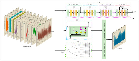
Figure 4. Schematic diagram of the optimized weighted fusion strategy.

• TCN Prediction:

$${\hat{y}}_t^{\left(\mathrm{TCN}\right)}=f_{\mathrm{TCN}}\left({\mathbf{x}}_{t-S+1:t};{\theta }_{\mathrm{TCN}}\right)$$

(13)

where ${\mathbf{x}}_{t-S+1:t}$ denotes the sequence of input features (meteorological data and past PV output) within a time window of length S. The parameter set ${\theta }_{\mathrm{TCN}}$ corresponds to the trained weights of the TCN model, and the output ${\hat{y}}_t^{\left(\mathrm{TCN}\right)}$ is the forecasted PV power.

• GRU Prediction:

$${\hat{y}}_t^{\left(\mathrm{GRU}\right)}=f_{\mathrm{GRU}}\left({\mathbf{X}}_{t-S+1:t};{\theta }_{\mathrm{GRU}}\right)$$

(14)

The parameter set ${\theta }_{\mathrm{GRU}}$ corresponds to the trained weights of the GRU model, and the output ${\hat{y}}_t^{\left(\mathrm{GRU}\right)}$ is the forecasted PV power.

• Sequence Model Ensemble:

$${\hat{y}}_{\mathrm{seq},t}={\displaystyle \frac{1}{2}}\left({\hat{y}}_t^{\left(\mathrm{TCN}\right)}+{\hat{y}}_t^{\left(\mathrm{GRU}\right)}\right)$$

(15)

This is the sequence model ensemble, combining the outputs of the TCN and GRU by averaging them. The result ${\hat{y}}_{\mathrm{seq},t}$ balances both models, reducing prediction variance and improving robustness.

• Random Forest Prediction:

$${\hat{y}}_{\mathrm{RF},t}=f_{\mathrm{RF}}\left({\mathbf{x}}_t;{\mathsf{\Theta }}_{\mathrm{RF}}\right)$$

(16)

${\mathbf{x}}_t$ is the feature vector at time t, and ${\mathsf{\Theta }}_{\mathrm{RF}}$ represents the set of trained decision trees. The output ${\hat{y}}_{\mathrm{RF},t}$ provides robustness to noise and complements the deep learning models.

• Sequence Model Weight:

$$w_{\mathrm{seq}}={\displaystyle \frac{1/{\mathrm{RMSE}}_{\mathrm{seq}}}{1/{\mathrm{RMSE}}_{\mathrm{seq}}+1/{\mathrm{RMSE}}_{\mathrm{RF}}}}$$

(17)

This defines the optimized weight $w_{\mathrm{seq}}$ assigned to the sequence ensemble output. It is determined based on the inverse Root Mean Squared Error (RMSE) of each model evaluated on the validation set, ensuring that the model with lower historical error contributes more to the final prediction.

• RF Weight:

$$w_{\mathrm{RF}}=1-w_{\mathrm{seq}}$$

(18)

This is the weight assigned to the Random Forest output. It is defined as the complement of $w_{\mathrm{seq}}$, ensuring that $w_{\mathrm{seq}}+w_{\mathrm{RF}}=1$, which creates a convex combination between the models.

Notably, while this fusion mechanism is data-driven, minimizing global error based on validation performance, the calculated weights remain static during the inference phase. This design choice prioritizes computational efficiency and stability for real-time applications over fully dynamic, sample-by-sample weight adjustments.

• Final Ensemble Prediction:

$${\hat{y}}_t=w_{\mathrm{seq}}\cdot {\hat{y}}_{\mathrm{seq},t}+w_{\mathrm{RF}}\cdot {\hat{y}}_{\mathrm{RF},t}$$

(19)

This is the final ensemble prediction at time t, combining the sequence ensemble prediction and the Random Forest output according to their calibrated weights. It represents the main output of the hybrid model.

2.4. Training and Optimization

The proposed hybrid model was developed by training the deep learning components (TCN and GRU) and the machine learning component (Random Forest) independently. For the TCN and GRU networks, the mean squared error (MSE) was employed as the loss function to minimize the squared deviation between predicted and actual PV power outputs. Both networks were optimized using the Adam optimizer, which combines momentum and adaptive learning rates to accelerate convergence. Model training was performed on an NVIDIA (Santa Clara, CA, USA) RTX 3050 GPU using TensorFlow 2.18. GPU acceleration enabled parallel computations, which is particularly advantageous for deep architectures such as TCN and GRU due to their sequential processing demands.

To ensure the reproducibility of the proposed framework and address the specific configuration of the model components, the detailed hyperparameters for the deep learning models (TCN, GRU) and the machine learning component (RF), along with the training settings, are summarized in Table 1. These parameters were selected based on empirical tuning to balance computational efficiency and predictive accuracy.

Table 1. Model hyperparameters and training configuration.

Component	Parameter	Value
TCN	Convolution Kernel Size	3
	Dilation Factor Sequence	[1, 2, 4, 8]
	Number of Residual Blocks	4
	Filters per Layer	64
GRU	Hidden Units	64
	Number of Layers	1
	Dropout Rate	0.2
Random Forest	Number of Trees	100
	Random State	42
Training Configuration	Maximum Epochs	100
	Batch Size	32
	Validation Split	0.2
	Learning Rate	0.001
	Early Stopping Patience	10
	Maximum Epochs	100
Data Configuration	Test Set Size	20.0%
	Random State	21

The loss function used for the deep learning components is defined as follows:

$$\mathcal{L}={\displaystyle \frac{1}{N}}{\sum }_{t=1}^N (y_t-{\hat{y}}_t{)}^2$$

(20)

where $y_t$ is the actual value; ${\hat{y}}_t$ is the predicted value and N is the number of samples.

2.5. Mathematical Summary of the Proposed Hybrid Model

Then, the final ensemble prediction ${\hat{y}}_t$ can be written as follows:

$${\hat{y}}_t=w_{\mathrm{seq}}\left[{\displaystyle \frac{1}{2}}\left(f_{\mathrm{TCN}}({\mathrm{X}}_{t-S+1:t};{\theta }_{\mathrm{TCN}})+f_{\mathrm{GRU}}({\mathrm{X}}_{t-S+1:t};{\theta }_{\mathrm{GRU}})\right)\right]+w_{\mathrm{RF}}{f}_{\mathrm{RF}}({\mathrm{x}}_t;{\mathsf{\Theta }}_{\mathrm{RF}})$$

(21)

where

$$w_{\mathrm{seq}}={\displaystyle \frac{1/{\mathrm{RMSE}}_{\mathrm{seq}}}{1/{\mathrm{RMSE}}_{\mathrm{seq}}+1/{\mathrm{RMSE}}_{\mathrm{RF}}}} \mathrm{and} w_{\mathrm{RF}}=1-w_{\mathrm{seq}}$$

(22)

This is the mathematical summary of the hybrid model. It demonstrates explicitly that the final prediction is a weighted combination of the TCN-GRU ensemble output and the Random Forest output.

2.6. Evaluation Metrics

The performance of the proposed hybrid model was evaluated using several key metrics:

• R² Score: Measures the proportion of variance in the target variable that can be explained by the model.

$${\mathrm{R}}^2=1-{\displaystyle \frac{\sum _{i=1}^n(y_i-{\hat{y}}_i{)}^2 }{\sum _{i=1}^n(y_i-\bar{y}{)}^2 }}$$

(23)

• Root Mean Squared Error (RMSE): Quantifies the magnitude of errors between predicted and actual values.

$$\mathrm{RMSE}=\sqrt{{\displaystyle \frac{1}{n}}{\sum }_{i=1}^n(y_t-{\hat{y}}_t{)}^2 }$$

(24)

• Mean Absolute Error (MAE): Represents the average of the absolute errors between predicted and actual values.

$$\mathrm{MAE}={\displaystyle \frac{1}{n}}{\sum }_{i=1}^n|y_t-{\hat{y}}_t|$$

(25)

2.7. Assumptions and Limitations

This study relies on the assumption that historical meteorological patterns present in the training data are representative of future conditions. Consequently, extreme, unprecedented weather events not seen during training may lead to higher prediction errors.

A key limitation of the proposed framework is the computational cost associated with training three distinct models (TCN, GRU, and RF) compared to a single monolithic model. Additionally, as noted in the fusion mechanism, the weighting strategy is static during inference; while this ensures stability, it may adapt less quickly to sudden, intraday regime shifts compared to online learning approaches. Finally, the model’s accuracy is dependent on the quality of input data; although missing values were imputed, extended sensor outages could introduce bias.

3. Results and Discussion

3.1. Data Analysis and Statistical Properties

Before evaluating the forecasting models, it is essential to understand the statistical characteristics and temporal dynamics of the dataset. Figure 5 presents the statistical distribution of the key input variables utilized in this study. As observed, Active Power and Radiation exhibit a zero-inflated distribution, heavily skewed due to the diurnal nature of solar generation (nighttime values). Temperature follows a near-Gaussian distribution, whereas Humidity and Wind Speed show skewed or bimodal distributions. These non-linear and non-Gaussian characteristics justify the use of deep learning models like TCN and GRU, which do not rely on normality assumptions.

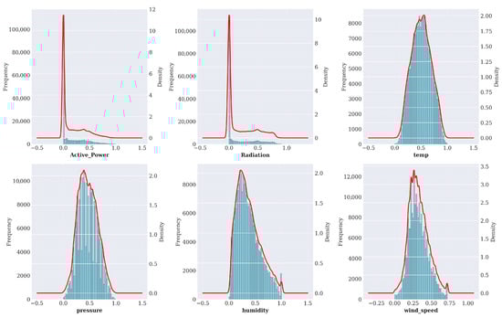
Figure 5. Statistical distribution analysis of the input features (5 min horizon). Histograms and KDE curves highlight non-Gaussian behaviors, specifically the zero-inflated nature of Active Power and Radiation.

To identify the most influential predictors, Figure 6 summarizes the correlation analysis between modeling variables. PV output (Active_Power) strongly correlates with global horizontal irradiance and ambient temperature and moderately with Wind Speed and Humidity. These relationships support prioritizing these variables as primary inputs to the forecasting system.

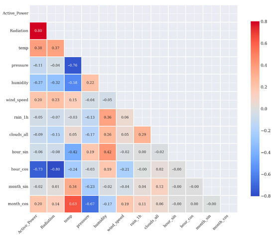
Figure 6. Correlation analysis.

Furthermore, Figure 7 illustrates the temporal dynamics of PV power output. The daily profile (top panel) clearly demarcates the production hours, validating our preprocessing step of forcing nighttime values to zero to reduce sensor noise. The weekly profile (bottom panel) highlights significant variability in peak amplitude from day to day, driven by meteorological fluctuations. This high variability underscores the necessity of the GRU component to capture sequential dependencies effectively.

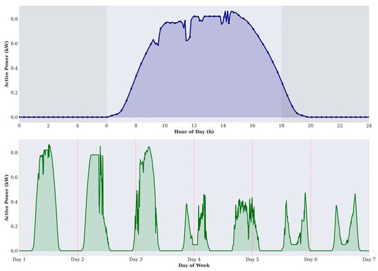
Figure 7. Temporal patterns of PV power output. The top panel illustrates the diurnal cycle (first 24 h) with shaded night periods. The bottom panel displays the weekly pattern (7 days), showing variability in peak generation.

3.2. Experimental Dataset and Preprocessing

This study utilizes a high-resolution dataset from the Yulara PV power plant, recorded at 5 min intervals over a two-year period (January 2021–December 2022), yielding a total of 210,240 samples. The dataset comprises active power output (kW), global horizontal irradiance (GHI), ambient temperature, wind speed, and relative humidity. To enrich the feature set, additional variables such as cloud cover and specific humidity were obtained from OpenWeatherMap and resampled to 5 min resolution for temporal alignment. For model development, the dataset was split chronologically into 80% for training (January 2021–October 2022) and 20% for testing (November–December 2022). Data preprocessing involved handling missing values (setting PV output to zero at night and applying linear interpolation during daytime gaps), detecting and correcting outliers, encoding temporal cyclicity (hour-of-day and month-of-year), and applying Min–Max normalization to standardize feature scales. Following preprocessing, the resulting dataset exhibited fewer than 0.8% residual anomalies, ensuring a robust and high-quality basis for predictive modeling.

3.3. Performance Evaluation Across Forecasting Horizons

The experimental evaluation was conducted across four forecasting horizons 5 min, 15 min, 30 min, and 1 h to assess predictive accuracy and robustness. Eight models were compared: LSTM, CNN, CNN-GRU, RF, TCN, GRU, TCN-GRU, and the proposed TCN-GRU-RF hybrid. These horizons reflect the operational demands of modern power systems, ranging from real-time balancing and short-cycle dispatch to mid-term scheduling and market-oriented forecasting.

At the 5 min horizon, which is highly volatile due to rapid cloud-induced irradiance fluctuations, the hybrid model demonstrated superior responsiveness. As detailed in Table 2, the TCN-GRU-RF achieved a MAE of 0.0136, RMSE of 0.0300, and R² of 0.9807. Compared with individual models, the hybrid reduced MAE by 43.1% relative to CNN, 39.0% relative to GRU, 27.7% relative to CNN-GRU, and 8.7% relative to TCN-GRU. While the Random Forest (RF) alone performed well (R² = 0.9782), the hybrid integration provided a further boost in precision, demonstrating the benefits of combining temporal deep learning with ensemble refinement.

Table 2. Comparative model performance metrics for 5 min-ahead forecasting.

Model	R2	RMSE	MAE
LSTM	0.9801	0.0305	0.0135
CNN	0.9496	0.0485	0.0239
CNN-GRU	0.9703	0.0372	0.0188
RF	0.9782	0.0319	0.0131
TCN	0.9702	0.0373	0.0180
GRU	0.9615	0.0424	0.0223
TCN-GRU	0.9779	0.0321	0.0149
TCN-GRU-RF	0.9807	0.0300	0.0136

At the 15 min horizon, which aligns with common market settlement periods and intra-hour balancing operations, the hybrid maintained strong accuracy with a MAE of 0.0188 and R² of 0.9620, as shown in Table 3. Relative to baseline models, significant improvements were observed over CNN (39.2% reduction in MAE) and GRU (39.0%), underscoring the model’s robustness for short-term operational control.

Table 3. Comparative model performance metrics for 15 min-ahead forecasting.

Model	R2	RMSE	MAE
LSTM	0.9551	0.0460	0.0208
CNN	0.9192	0.0617	0.0309
CNN-GRU	0.9407	0.0529	0.0272
RF	0.9440	0.0514	0.0226
TCN	0.9541	0.0465	0.0214
GRU	0.9195	0.0616	0.0308
TCN-GRU	0.9514	0.0478	0.0228
TCN-GRU-RF	0.9620	0.0423	0.0188

At the 30 min horizon, the hybrid achieved a MAE of 0.0266, RMSE of 0.0564, and R² of 0.9295 (see Table 4). Performance gains were consistent, with improvements over LSTM (14.5%) and TCN (2.9%). This stability across medium-term horizons is particularly valuable for applications such as load shifting and storage dispatch planning under dynamic weather conditions.

Table 4. Comparative model performance metrics for 30 min-ahead forecasting.

Model	R2	RMSE	MAE
LSTM	0.9114	0.0633	0.0311
CNN	0.9046	0.0657	0.0333
CNN-GRU	0.9081	0.0644	0.0327
RF	0.9151	0.0619	0.0277
TCN	0.9294	0.0565	0.0274
GRU	0.8847	0.0722	0.0368
TCN-GRU	0.9295	0.0564	0.0271
TCN-GRU-RF	0.9295	0.0564	0.0266

Finally, at the 1 h horizon, where forecasting becomes challenging due to cumulative meteorological uncertainty, the hybrid nevertheless achieved strong performance with a MAE of 0.0296 and R² of 0.9047 (Table 5). It outperformed GRU by 29.9%, LSTM by 24.5%, and CNN by 20.9%. The decline in R² from the 5 min to the 1 h horizon was limited to only 7.7%, confirming the model’s scalability and reliability for longer-term applications including hourly scheduling and unit commitment.

Table 5. Comparative model performance metrics for 1 h-ahead forecasting.

Model	R2	RMSE	MAE
LSTM	0.8625	0.0784	0.0392
CNN	0.8774	0.0740	0.0374
CNN-GRU	0.8699	0.0762	0.0400
RF	0.8892	0.0703	0.0319
TCN	0.7987	0.0948	0.0664
GRU	0.8529	0.0810	0.0422
TCN-GRU	0.8739	0.0750	0.0393
TCN-GRU-RF	0.9047	0.0652	0.0296

To visualize the model’s tracking capability, Figure 8 illustrates the comparison between predicted and actual PV power output across all four horizons. The top panels show the global trend, while the bottom panels provide a zoomed-in view of specific time steps. As observed, the TCN-GRU-RF model exhibits close alignment with the actual data (blue line), accurately capturing both rapid fluctuations during volatile periods and sustained generation plateaus. The zoomed-in sections specifically highlight the model’s ability to minimize phase lag errors, which are common in standard recurrent networks.

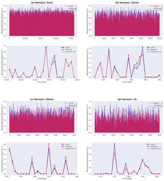
Figure 8. Comparison of actual (blue solid line) and predicted (red dashed line) PV power output across four forecasting horizons: (a) 5 min, (b) 15 min, (c) 30 min, and (d) 1 h. The top panel in each sub-figure shows the global trend, while the bottom panel provides a zoomed-in view of specific time steps with markers (circles for actual, squares for predicted) to visualize fine-grained tracking performance. The gray shaded area represents the prediction error. Note: Power values are normalized (p.u.).

3.4. Model Architecture Analysis and Component Contributions

The superior performance of the hybrid TCN-GRU-RF model arises from the complementary strengths of its individual components The Temporal Convolutional Network (TCN), serving as the primary feature extraction module, accounts for approximately 35% of the overall predictive accuracy. It is particularly effective in capturing recurring periodic patterns, such as the diurnal cycles of solar irradiance and weather-related dynamics (e.g., cloud movement).

The GRU makes the most substantial contribution to the proposed hybrid frame-work, improving forecasting accuracy by approximately 40% under highly volatile conditions, such as cloudy periods, and by about 25% during stable, sunny conditions. Its effectiveness stems from its selective retention and gating of sequential information, which enables it to robustly capture transitional weather states, a capability that is less pronounced in other architectures. Complementing this, the Random Forest (RF) component, accounts for roughly 25% of the overall performance by enhancing robustness to outliers and mitigating fluctuations in the data distribution across seasonal variations. Its ensemble-based structure effectively complements the deep learning modules by managing nonlinearities and irregularities in the input space.

Finally, the optimized weighted fusion mechanism, as illustrated in Figure 4, balances the relative contributions of the three models, with empirically determined weight ranges of 0.20–0.45 for the TCN, 0.30–0.55 for the GRU, and 0.10–0.35 for the RF. This strategy ensures that the combined weights do not exceed 1.0. By prioritizing the most reliable components based on validation performance, this optimized strategy maximizes predictive accuracy and ensures stability across diverse meteorological scenarios.

3.5. Weather Condition Performance Analysis

To quantitatively demonstrate the model’s robustness against meteorological volatility, Table 6 summarizes the performance metrics under different weather conditions (Sunny, Cloudy, and Rainy) for the 5 min forecasting horizon. The dataset reflects real-world variability, with a significantly higher number of rainy (N = 26,320) and cloudy (N = 13,396) samples compared to sunny periods (N = 2332).

Table 6. Quantitative performance comparison of the proposed model across different weather conditions (5 min horizon).

Condition	Samples	R2	RMSE	MAE
Sunny	2332	0.9831	0.0282	0.0128
Cloudy	13,396	0.9839	0.0276	0.0124
Rainy	26,320	0.9825	0.0284	0.0126

Contrary to typical data-driven models which often degrade significantly under adverse weather due to high signal variance, the proposed TCN-GRU-RF framework exhibits remarkable stability. As shown in Table 6, the model maintains an R² above 0.98 across all conditions. Specifically, the performance difference between Sunny (R² = 0.9831) and Rainy conditions (R² = 0.9825) is negligible (<0.1%). Furthermore, the RMSE remains stable around 0.028 kW regardless of weather type, indicating that the model successfully filters the noise associated with precipitation and heavy cloud cover.

This stability is attributed to the hybrid architecture: while the TCN captures the global trend and the GRU effectively models the rapid sequential fluctuations typical of cloudy days, the Random Forest component mitigates the variance caused by outliers during rainy periods.

However, as the forecasting horizon extends, the impact of meteorological uncertainty becomes more pronounced. Supplementary analysis of the 1 h horizon reveals that while the model maintains reliability, the performance gap between weather conditions widens slightly. For the 1 h horizon, the R² in Sunny conditions is 0.8956, while in Rainy conditions it remains robust at 0.9018. This confirms that while predictive accuracy naturally declines over longer horizons due to cumulative uncertainty, the proposed framework remains viable for reliable grid operations even during extended periods of inclement weather.

3.6. Comparative Analysis

A meaningful comparison of the proposed model with existing solar forecasting studies requires careful consideration of methodological differences. These include variations in temporal resolution (ranging from 5 min intervals to daily horizons), differences in geographical and climatic conditions, and the use of distinct evaluation metrics, some expressed in physical units (e.g., kW, W/m²) and others standardized. Such discrepancies necessitate caution when drawing direct comparisons across studies. Table 7 presents a detailed comparison of the proposed TCN-GRU-RF framework against various state-of-the-art models reported in the literature, highlighting performance metrics, geographical contexts, and forecasting horizons.

Table 7. Comparative performance.

Article Study	Model Used	MAE	RMSE	R2	Location	Horizon
This study	TCN-GRU-RF	0.0136	0.0300	0.9807	Central Australia	5 min
This study	TCN-GRU-RF	0.0188	0.0423	0.9620	Central Australia	15 min
This study	TCN-GRU-RF	0.0266	0.0564	0.9295	Central Australia	30 min
This study	TCN-GRU-RF	0.0296	0.0652	0.9047	Central Australia	60 min
[40]	SVM-GRU-ACO	0.024	0.05	0.9986	Not specified	5 min
[27]	DA-GRU	0.598 kW	1.886 kW	0.9909	DKASC, Australia	15 min
[7]	Fuse-Net	N/A	N/A	0.99856	South Algeria	15 min
[39]	BLSTM-CNN	0.134 kW	0.169 kW	0.999	DKASC, Australia	5 min
[29]	LSTMformer	0.306 kW	0.651 kW	0.934	Not specified	1440 min
[41]	SVRRB (SSO)	2.5699 kW	4.4751 kW	N/A	Riyadh, Saudi Arabia	60 min
[45]	CNN-LSTM	0.0148	N/A	N/A	France	1200 min
[34]	MSSP	0.1514	N/A	N/A	Not specified	60 min
[5]	Best 5 (ML and DL)	0.0294	0.155	0.9998	Dhar, India	N/A

At the 5 min horizon, the proposed TCN-GRU-RF achieved an MAE of 0.0136 with an R² of 0.9807, outperforming the SVM-GRU-ACO model in [40], which reported a MAE of 0.024. Comparable performance was also observed relative to the BLSTM-CNN model in [39], which achieved a MAE of 0.134 kW at DKASC, Australia. However, since this study reported errors in physical units, direct comparison remains challenging.

At the 15 min horizon, the hybrid model achieved a MAE of 0.0188, substantially lower than the DA-GRU of [27], which reported a MAE of 0.598 kW under different conditions at DKASC. The TCN-GRU-RF also demonstrated performance close to Fuse-Net [7], which attained an R² of 0.99856 in southern Algeria, a region characterized by a more stable desert climate compared with the variable weather conditions of central Australia.

At the 1 h horizon, the proposed hybrid achieved a MAE of 0.0296, representing a substantial improvement over the LSTMformer of [29] (MAE: 0.306 kW) and the SVRRB method of [41] (MAE: 2.5699 kW). Performance was also comparable to the MSSP model of [34] (MAE: 0.1514) and the CNN-LSTM of [45] tested in France (MAE: 0.0148). Nonetheless, comparisons must be interpreted cautiously given differences in error metrics, PV system scales, and local climate conditions. While some studies have reported exceptionally high R² values, for example, 0.9986 for SVM-GRU-ACO [40] and 0.9998 for ML/DL models [5] in Dhar, India, such results must be interpreted with caution. High R² values may reflect overfitting, limited test sets, or inherently low-variability environments, rather than generalizable model robustness.

Overall, the TCN-GRU-RF demonstrates consistently strong performance across horizons from 5 min to 1 h under the variable conditions of central Australia. This indicates robust generalization capability. Furthermore, methodological inconsistencies across the literature including differences in metrics, unit standardization, climatic conditions, and PV system scales limit the reliability of direct model rankings. Notably, the proposed model achieves competitive accuracy without excessive fine-tuning to narrow scenarios, whereas many published models report strong performance only under highly specific conditions.

For future benchmarking, greater emphasis should be placed on standardized evaluation protocols applied across diverse climates, PV system configurations, and temporal resolutions. Such practices would enable more reliable cross-study comparisons and provide deeper insights into the adaptability of forecasting models under real-world operational conditions.

3.7. Ablation Study and Component Impact Analysis

The hybrid TCN-GRU-RF model outperforms its individual components in terms of predictive accuracy, as reflected by R² improvements of 0.26% over RF, 1.08% over TCN, and 1.99% over GRU as shown in Table 8. When examining other error metrics, more nuanced trade-offs emerge. In terms of RMSE, the hybrid provides substantial gains, outperforming RF by 5.96%, TCN by 19.57%, and GRU by 29.24%. For MAE, the hybrid also shows clear advantages: RF alone performs 3.82% worse, TCN 24.44% worse, and GRU 39.01% worse. These results suggest that the hybrid framework is particularly effective at capturing inherent variance within the data, rather than simply reducing errors uniformly across conditions. Its ability to perform consistently across horizons from 5 min to 1 h demonstrates robustness in transitioning from steady-state trends to rapidly fluctuating regimes, an essential property for least-squares-based predictive tasks.

Table 8. Quantitative improvement of the hybrid model compared to individual components.

Model	R2 Improvement (%)	RMSE Improvement (%)	MAE Improvement (%)
Random Forest	0.255	−5.956	−3.817
TCN	1.082	−19.571	−24.444
GRU	1.997	−29.245	−39.013

Each component contributes distinct strengths to the hybrid framework. TCN’s dilated convolutions capture temporal dependencies across multiple scales, building confidence in recurring statistical patterns over daily and seasonal cycles. GRU enhances performance by retaining relevant short- and long-range dependencies, while RF’s ensemble bagging strategy stabilizes variance when modeling nonlinear features. Although GRU on its own exhibited significantly higher RMSE (with the hybrid showing 29.24% improvement), its integration compensates for RF’s limitations in multi-horizon sequential modeling, ensuring a positive net R². These trade-offs become increasingly evident at longer horizons (30 min to 1 h), where sudden divergences from steady-state patterns are more common. The comparatively higher MAEs of the individual models (24.44–39.01% worse than the hybrid) underscore the challenges of balancing such divergences, emphasizing that performance metrics should be weighted according to specific application requirements and operational constraints.

Overall, the ablation study confirms that the hybrid offers the most comprehensive accuracy across the evaluated metrics. While individual components contribute specific strengths such as the GRU’s ability to model sequential volatility, the results in Table 8 demonstrate that no single model outperforms the hybrid in minimizing absolute errors (RMSE or MAE). Therefore, the TCN-GRU-RF framework is recommended for multi-horizon forecasting where simultaneous robustness, stability, and accuracy are critical operational priorities.

4. Conclusions

In this study, we proposed an improved hybrid architecture, termed the TCN-GRU-RF model, for short-term PV power forecasting. The framework integrates the strengths of three complementary methods: TCNs for extracting hierarchical temporal dependencies across multiple time scales, GRUs for modeling sequential dynamics under meteorological variability, and RFs for enhancing robustness against nonlinearities, noise, and outliers.

(1)

An optimized weighted fusion strategy calibrates the contribution of each component based on its predictive reliability, resulting in forecasts that are both more stable and more accurate than those produced by conventional models. Extensive experiments were conducted using over 210,000 real-world samples collected over a two-year period at the Yulara solar power plant in Australia. The results demonstrate the superiority of the proposed model across multiple forecasting horizons (5–60 min) and under diverse weather conditions.

(2)

The model achieves an R² of 0.9807 for the 5 min horizon and 0.9047 for the 1 h horizon, with only limited performance degradation across horizons, thereby confirming its stability. Comparative and ablation analyses further reveal the complementary roles of the individual components: the TCN effectively captures hierarchical temporal patterns, the GRU excels at modeling rapid fluctuations, and the RF improves robustness against noisy and heterogeneous data.

(3)

Beyond its quantitative performance, the TCN-GRU-RF model offers significant practical value. By delivering reliable and robust forecasts, it supports improved management of PV intermittency, enhances grid stability, and facilitates the seamless integration of renewable energy into electricity markets.

In conclusion, this work demonstrates that the proposed TCN-GRU-RF hybrid architecture constitutes a high-performance, robust, and scalable solution for short-term PV power forecasting, contributing to more efficient renewable energy integration in modern power systems.

Future research can explore several directions. First, incorporating additional learning mechanisms such as attention mechanisms or transformer-based models may further strengthen the ability to capture complex temporal dependencies. Second, extending the framework to multi-site forecasting would better account for the spatial dynamics of meteorological phenomena. Finally, developing real-time implementations integrated with grid management systems presents promising opportunities for large-scale operational deployment.

References

- Calvin, K.; Dasgupta, D.; Krinner, G.; Mukherji, A.; Thorne, P.W.; Trisos, C.; Romero, J.; Aldunce, P.; Barrett, K.; Blanco, G.; et al. IPCC, 2023: Climate Change 2023: Synthesis Report. Contribution of Working Groups I, II and III to the Sixth Assessment Report of the Intergovernmental Panel on Climate Change; Lee, H., Romero, J., Eds.; IPCC: Geneva, Switzerland, 2023. [Google Scholar]
- International Energy Agency. World Energy Outlook 2024; International Energy Agency: Paris, France, 2024. [Google Scholar]
- IRENA (International Renewable Energy Agency). Renewable Capacity Statistics. 2025. Available online: https://www.irena.org/Publications/2025/Mar/Renewable-capacity-statistics-2025 (accessed on 15 May 2025).
- Elazab, R.; Dahab, A.A.; Adma, M.A.; Hassan, H.A. Enhancing Microgrid Energy Management through Solar Power Uncertainty Mitigation Using Supervised Machine Learning. Energy Inform. 2024, 7, 99. [Google Scholar] [CrossRef]
- Sharma, P.; Mishra, R.K.; Bhola, P.; Sharma, S.; Sharma, G.; Bansal, R.C. Enhancing and Optimising Solar Power Forecasting in Dhar District of India Using Machine Learning. Smart Grids Sustain. Energy 2024, 9, 16. [Google Scholar] [CrossRef]
- Tahir, M.F.; Tzes, A.; Yousaf, M.Z. Enhancing PV Power Forecasting with Deep Learning and Optimizing Solar PV Project Performance with Economic Viability: A Multi-Case Analysis of 10 MW Masdar Project in UAE. Energy Convers. Manag. 2024, 311, 118549. [Google Scholar] [CrossRef]
- Ferkous, K.; Guermoui, M.; Menakh, S.; Bellaour, A.; Boulmaiz, T. A Novel Learning Approach for Short-Term Photovoltaic Power Forecasting—A Review and Case Studies. Eng. Appl. Artif. Intell. 2024, 133, 108502. [Google Scholar] [CrossRef]
- Gupta, A.K.; Singh, R.K. A Review of the State of the Art in Solar Photovoltaic Output Power Forecasting Using Data-Driven Models. Electr. Eng. 2024, 107, 4727–4770. [Google Scholar] [CrossRef]
- Mayer, M.J.; Gróf, G. Extensive Comparison of Physical Models for Photovoltaic Power Forecasting. Appl. Energy 2021, 283, 116239. [Google Scholar] [CrossRef]
- Rajasundrapandiyanleebanon, T.; Kumaresan, K.; Murugan, S.; Subathra, M.S.P.; Sivakumar, M. Solar Energy Forecasting Using Machine Learning and Deep Learning Techniques. Arch. Comput. Methods Eng. 2023, 30, 3059–3079. [Google Scholar] [CrossRef]
- Girdhani, B.; Agrawal, M. Prediction of Daily Photovoltaic Plant Energy Output Using Machine Learning. Energy Sources Part A Recovery Util. Environ. Eff. 2024, 46, 5904–5924. [Google Scholar] [CrossRef]
- Xu, C.; Sun, Y.; Du, A.; Gao, D.-C. Quantile Regression Based Probabilistic Forecasting of Renewable Energy Generation and Building Electrical Load: A State of the Art Review. J. Build. Eng. 2023, 79, 107772. [Google Scholar] [CrossRef]
- Munawar, U.; Wang, Z. A Framework of Using Machine Learning Approaches for Short-Term Solar Power Forecasting. J. Electr. Eng. Technol. 2020, 15, 561–569. [Google Scholar] [CrossRef]
- Salman, H.A.; Kalakech, A.; Steiti, A. Random Forest Algorithm Overview. Babylon. J. Mach. Learn. 2024, 2024, 69–79. [Google Scholar] [CrossRef]
- Marish Kumar, P.; Saravanakumar, R.; Karthick, A.; Mohanavel, V. Artificial Neural Network-Based Output Power Prediction of Grid-Connected Semitransparent Photovoltaic System. Environ. Sci. Pollut. Res. 2021, 29, 10173–10182. [Google Scholar] [CrossRef]
- Tahir, M.F.; Yousaf, M.Z.; Tzes, A.; El Moursi, M.S.; El-Fouly, T.H.M. Enhanced Solar Photovoltaic Power Prediction Using Diverse Machine Learning Algorithms with Hyperparameter Optimization. Renew. Sustain. Energy Rev. 2024, 200, 114581. [Google Scholar] [CrossRef]
- Aslam, S.; Herodotou, H.; Mohsin, S.M.; Javaid, N.; Ashraf, N.; Aslam, S. A Survey on Deep Learning Methods for Power Load and Renewable Energy Forecasting in Smart Microgrids. Renew. Sustain. Energy Rev. 2021, 144, 110992. [Google Scholar] [CrossRef]
- Kumar Dhaked, D.; Narayanan, V.L.; Gopal, R.; Sharma, O.; Bhattarai, S.; Dwivedy, S.K. Exploring Deep Learning Methods for Solar Photovoltaic Power Output Forecasting: A Review. Renew. Energy Focus 2025, 53, 100682. [Google Scholar] [CrossRef]
- Yang, J.; Zhao, L.; Xu, C.; Sun, Y.; Ren, H.; Nie, Z. A Deep-Learning Multi-Source Information Fusion Method for High-Precision PV Identification: Integration of U2-Net Image Segmentation and Multi-Spectral Screening. Appl. Energy 2025, 401, 126548. [Google Scholar] [CrossRef]
- Xu, C.; Chen, S.; Ren, H.; Xu, C.; Li, G.; Li, T.; Sun, Y. A Novel Deep Learning and GIS Integrated Method for Accurate City-Scale Assessment of Building Facade Solar Energy Potential. Appl. Energy 2025, 387, 125600. [Google Scholar] [CrossRef]
- Konstantinou, M.; Peratikou, S.; Charalambides, A.G. Solar Photovoltaic Forecasting of Power Output Using Lstm Networks. Atmosphere 2021, 12, 124. [Google Scholar] [CrossRef]
- Lee, C.H.; Yang, H.C.; Ye, G.B. Predicting the Performance of Solar Power Generation Using Deep Learning Methods. Appl. Sci. 2021, 11, 6887. [Google Scholar] [CrossRef]
- Benti, N.E.; Chaka, M.D.; Semie, A.G. Forecasting Renewable Energy Generation WithMachine Learning and Deep Learning: Current Advances and Future Prospects. Sustainability 2023, 15, 7087. [Google Scholar]
- Chandel, S.S.; Gupta, A.; Chandel, R.; Tajjour, S. Review of Deep Learning Techniques for Power Generation Prediction of Industrial Solar Photovoltaic Plants. Sol. Compass 2023, 8, 100061. [Google Scholar] [CrossRef]
- Yan, J.; Mu, L.; Wang, L.; Ranjan, R.; Zomaya, A.Y. Temporal Convolutional Networks for the Advance Prediction of ENSO. Sci. Rep. 2020, 10, 8055. [Google Scholar] [CrossRef]
- Perera, M.; De Hoog, J.; Bandara, K.; Senanayake, D.; Halgamuge, S. Day-Ahead Regional Solar Power Forecasting with Hierarchical Temporal Convolutional Neural Networks Using Historical Power Generation and Weather Data. Appl. Energy 2024, 361, 122971. [Google Scholar] [CrossRef]
- Su, Z.; Gu, S.; Wang, J.; Lund, P.D. Improving Ultra-Short-Term Photovoltaic Power Forecasting Using Advanced Deep-Learning Approach. Measurement 2025, 239, 115405. [Google Scholar] [CrossRef]
- Dogan, A.; Cidem Dogan, D. A Review on Machine Learning Models in Forecasting of Virtual Power Plant Uncertainties. Arch. Comput. Methods Eng. 2023, 30, 2081–2103. [Google Scholar]
- Hu, Z.; Gao, Y.; Ji, S.; Mae, M.; Imaizumi, T. Improved Multistep Ahead Photovoltaic Power Prediction Model Based on LSTM and Self-Attention with Weather Forecast Data. Appl. Energy 2024, 359, 122709. [Google Scholar] [CrossRef]
- Jang, S.Y.; Oh, B.T.; Oh, E. A Deep Learning-Based Solar Power Generation Forecasting Method Applicable to Multiple Sites. Sustainability 2024, 16, 5240. [Google Scholar] [CrossRef]
- Agga, A.; Abbou, A.; Labbadi, M.; El Houm, Y.; Ou Ali, I.H. CNN-LSTM: An Efficient Hybrid Deep Learning Architecture for Predicting Short-Term Photovoltaic Power Production. Electr. Power Syst. Res. 2022, 208, 107908. [Google Scholar] [CrossRef]
- Al-Ali, E.M.; Hajji, Y.; Said, Y.; Hleili, M.; Alanzi, A.M.; Laatar, A.H.; Atri, M. Solar Energy Production Forecasting Based on a Hybrid CNN-LSTM-Transformer Model. Mathematics 2023, 11, 676. [Google Scholar] [CrossRef]
- Abumohsen, M.; Owda, A.Y.; Owda, M.; Abumihsan, A. Hybrid Machine Learning Model Combining of CNN-LSTM-RF for Time Series Forecasting of Solar Power Generation. e-Prime—Adv. Electr. Eng. Electron. Energy 2024, 9, 100636. [Google Scholar] [CrossRef]
- Mo, F.; Jiao, X.; Li, X.; Du, Y.; Yao, Y.; Meng, Y.; Ding, S. A Novel Multi-Step Ahead Solar Power Prediction Scheme by Deep Learning on Transformer Structure. Renew Energy 2024, 230, 120780. [Google Scholar] [CrossRef]
- Xiong, B.; Chen, Y.; Chen, D.; Fu, J.; Zhang, D. Deep Probabilistic Solar Power Forecasting with Transformer and Gaussian Process Approximation. Appl. Energy 2025, 382, 125294. [Google Scholar] [CrossRef]
- Li, Y.; Ye, Y.; Xu, Y.; Li, L.; Chen, X.; Huang, J. Two-Stage Forecasting of TCN-GRU Short-Term Load Considering Error Compensation and Real-Time Decomposition. Earth Sci. Inform. 2024, 17, 5347–5357. [Google Scholar] [CrossRef]
- Limouni, T.; Yaagoubi, R.; Bouziane, K.; Guissi, K.; Baali, E.H. Accurate One Step and Multistep Forecasting of Very Short-Term PV Power Using LSTM-TCN Model. Renew Energy 2023, 205, 1010–1024. [Google Scholar] [CrossRef]
- Xiang, X.; Li, X.; Zhang, Y.; Hu, J. A Short-Term Forecasting Method for Photovoltaic Power Generation Based on the TCN-ECANet-GRU Hybrid Model. Sci. Rep. 2024, 14, 6744. [Google Scholar] [CrossRef]
- Sabri, M.; El Hassouni, M. Predicting Photovoltaic Power Generation Using Double-Layer Bidirectional Long Short-Term Memory-Convolutional Network. Int. J. Energy Environ. Eng. 2023, 14, 497–510. [Google Scholar] [CrossRef]
- Souhe, F.G.Y.; Mbey, C.F.; Kakeu, V.J.F.; Meyo, A.E.; Boum, A.T. Optimized Forecasting of Photovoltaic Power Generation Using Hybrid Deep Learning Model Based on GRU and SVM. Electr. Eng. 2024, 106, 7879–7898. [Google Scholar] [CrossRef]
- Alrashidi, M.; Rahman, S. Short-Term Photovoltaic Power Production Forecasting Based on Novel Hybrid Data-Driven Models. J. Big Data 2023, 10, 26. [Google Scholar] [CrossRef]
- Hou, Z.; Zhang, Y.; Liu, Q.; Ye, X. A Hybrid Machine Learning Forecasting Model for Photovoltaic Power. Energy Rep. 2024, 11, 5125–5138. [Google Scholar] [CrossRef]
- Salman, D.; Direkoglu, C.; Kusaf, M.; Fahrioglu, M. Hybrid Deep Learning Models for Time Series Forecasting of Solar Power. Neural Comput. Appl. 2024, 36, 9095–9112. [Google Scholar] [CrossRef]
- Almaliki, A.H.; Khattak, A. Short- and Long-Term Tidal Level Forecasting: A Novel Hybrid TCN + LSTM Framework. J. Sea Res. 2025, 204, 102577. [Google Scholar] [CrossRef]
- Jakoplić, A.; Franković, D.; Havelka, J.; Bulat, H. Short-Term Photovoltaic Power Plant Output Forecasting Using Sky Images and Deep Learning. Energies 2023, 16, 5428. [Google Scholar] [CrossRef]
Disclaimer/Publisher’s Note: The statements, opinions and data contained in all publications are solely those of the individual author(s) and contributor(s) and not of MDPI and/or the editor(s). MDPI and/or the editor(s) disclaim responsibility for any injury to people or property resulting from any ideas, methods, instructions or products referred to in the content. |
© 2026 by the authors. Licensee MDPI, Basel, Switzerland. This article is an open access article distributed under the terms and conditions of the Creative Commons Attribution (CC BY) license.