GPU-Accelerated Deep Learning Algorithms for MIMO Signal Detection

Abstract

Deep learning (DL) has emerged as a promising alternative for signal detection in multiple-input multiple-output (MIMO) wireless communication systems, achieving a performance close to the optimal maximum likelihood (ML) criterion. However, implementing DL algorithms for MIMO signal detection still demands a high computational cost. Recently, a DL-based architecture with reduced complexity was proposed for MIMO signal detection. More specifically, a preprocessing stage was added to label the input signals, resulting in a more efficient detection scheme. However, even with this reduction in complexity, the proposed detection schemes remain computationally demanding, and this cost grows sharply as the system scales to higher-order modulations and/or large antenna arrays. To further reduce the complexity of these schemes, this paper proposes a graphics processing unit (GPU)-accelerated procedure for DL-based MIMO signal detection. The algorithm is accelerated by using two strategies in a CUDA-enabled PyTorch implementation. First, we optimize the training, which tightens the bit error rate (BER) gap from 1.00 dB to approximately 0.20 dB for the One-Hot (OH) labeling and from 2.00 dB to approximately 0.90 dB for the One-Hot-per-Antenna (OHA) labeling. Additionally, we optimize the Monte Carlo simulation using seven strategies, reducing the end-to-end evaluation time by 34.7% on an NVIDIA RTX 4090 GPU. These results aim to support future projects in evaluating DL-based MIMO systems using shorter computing windows.

1. Introduction

Multiple-input multiple-output (MIMO) systems are a key enabling technology for beyond fifth-generation (5G) and sixth-generation (6G) wireless communications systems, delivering substantial gains in data rate and spectral efficiency. Signal detection, however, remains one of their main bottlenecks. The optimal maximum likelihood (ML) criterion performs an exhaustive search over the transmitted alphabet, so its complexity grows as $M^{N_t}$, where M is the modulation order and $N_t$ the number of transmit antennas. This exponential dependence makes optimal detection impractical for moderate or large MIMO configurations. The theoretical advantages of MIMO systems lie in their capacity gains [1,2]. Under a Rayleigh fading channel, the spectral efficiency scales linearly with $min(N_t,N_r)$, rather than logarithmically as in single-antenna systems. That multiplexing gain motivated the massive-MIMO paradigm introduced by Marzetta [3], where a base station deploys a large excess of antennas over simultaneously served users. Scaling to such configurations amplifies the already prohibitive ML complexity to the point where it becomes purely theoretical. Among the suboptimal alternatives, sphere decoding achieves near-optimal performance [4,5]. However, its average complexity degrades at low SNR, where the search radius admits more candidates inside the sphere [5].

In light of this, deep learning (DL) has emerged as a qualitatively different way of tackling this problem [6,7]. O’Shea and Hoydis [8] formalized this direction by interpreting an end-to-end communication system as an autoencoder trained jointly over a transmitter (Tx) and a receiver (Rx); subsequent works have applied a similar principle to channel estimation [9] and, more broadly, to other communication tasks, including automatic modulation classification, signal detection in large-scale MIMO [10], and radio resource allocation [11]. Once trained, a neural network approximates the ML criterion at a fraction of its cost, and its performance can be tuned explicitly via the labeling strategy applied to the transmitted symbols [12,13,14,15,16].

Recently, an efficient, DL-based MIMO detection scheme was proposed in [15], where the proposed strategy incorporates an additional preprocessing stage and compares two novel encoding strategies: One-Hot-per-Antenna (OHA), and Direct Symbol Encoding (DSE), showing that the OHA and DSE strategies reach an F1-score of 0.97 with losses in bit error rate (BER) below 1 dB and 2 dB, respectively, and with a reduced complexity compared with the conventional One-Hot (OH) strategy. However, in this previous work, two aspects remain relatively underexplored. First, the sensitivity of BER performance to the training configuration: amount of data, number of epochs, and output-layer activation. Second, the cost of the Monte Carlo evaluation itself, which in a $2\times 2$ MIMO configuration with ${10}^6$ iterations per each signal-to-noise ratio (SNR) point could consume more than seventeen hours, even on a modern graphics processing unit (GPU) such as the NVIDIA RTX 4090. To address this issue, this work proposes a GPU-accelerated procedure utilizing a CUDA-enabled PyTorch (Ver. 2.5.0+cu121) [17]. framework implemented on an NVIDIA RTX 4090 GPU. Unlike the reference work, which proposes the labeling strategies, this work does not introduce a new detector but reproduces that scheme on GPU and focuses on accelerating its evaluation: the larger training budget afforded by the GPU brings the OH and OHA schemes closer to the ML detector, reducing the BER gap from 1.00 dB to approximately 0.20 dB for OH and from 2.00 dB to approximately 0.90 dB for OHA, while seven optimizations of the Monte Carlo simulation reduce the end-to-end evaluation time by 34.7%. The contributions of this work are:

• An optimized training framework for the three labeling strategies in [15], evaluated in terms of accuracy, F1-score, and BER performance.
• Seven algorithmic optimizations of the Monte Carlo simulation that reduce a full end-to-end evaluation time by 34.7% without affecting the BER performance.
• A discussion of the theoretical multiplicative ceiling versus the measured real speedup, framed through Amdahl’s law [18].

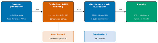
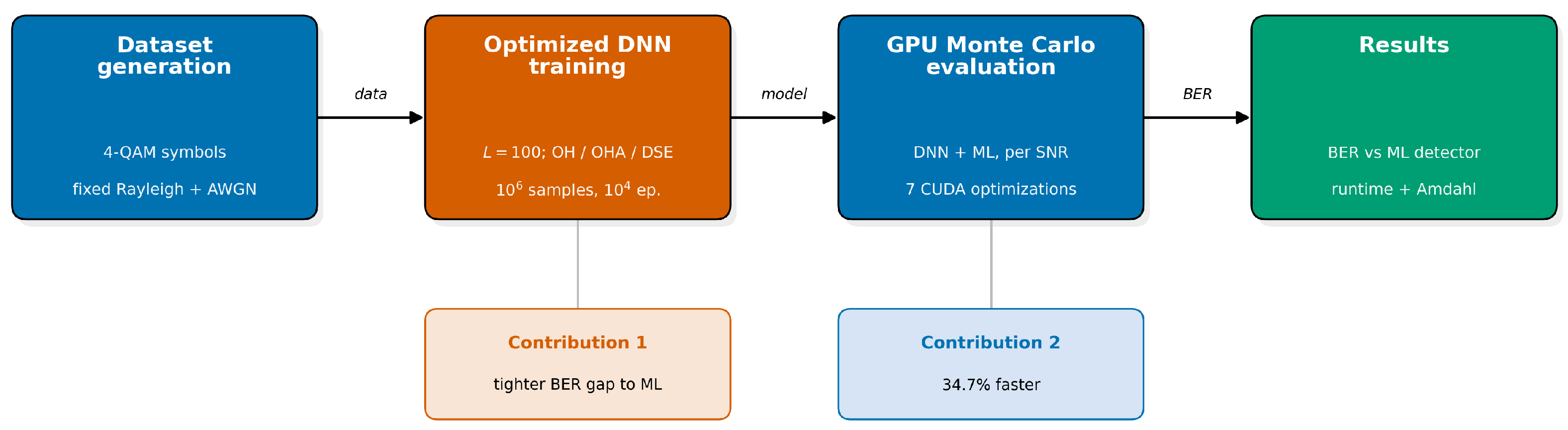
Figure 1 provides a high-level block diagram of the complete proposed design, from dataset generation through the optimized training and the GPU-accelerated Monte Carlo evaluation to the reported BER and runtime results, so the overall process can be followed before the individual components are detailed.

Figure 1. Block diagram of the complete proposed design: dataset generation, optimized DNN training (Contribution 1), GPU-accelerated Monte Carlo BER evaluation with the seven optimizations (Contribution 2), and the reported results.

The remainder of the paper is organized as follows. Section 2 summarizes the background on MIMO detection and deep learning. Section 3 presents the system model. Section 4 describes the training framework and Section 5 the seven optimizations, and the measurement methodology. The results are grouped in Section 6, where the applicability, advantages, limitations, and additional context of the proposed framework are discussed. Conclusions are given in Section 7.

Notation: Bold-face lowercase letters and bold-face uppercase letters indicate vectors and matrices, respectively. The notations ${(·)}^T$, ${(·)}^H$, and $\parallel ·\parallel$ indicate the transpose, the conjugate transpose, and the norm of a vector or matrix. The Gaussian distribution of a complex variable with mean $\mu$ and ${\sigma }^2$ variance is denoted as $\mathcal{N}(\mu ,{\sigma }^2)$.

2. Signal Detection in MIMO Systems

Classical MIMO detection spans a spectrum of trade-offs between complexity and performance. At one end, the zero-forcing (ZF) and minimum mean square error (MMSE) detectors are linear and cheap; they typically degrade by several decibels compared to the ML detector in fading channels [19,20]. At the other end, the ML detector solves the detection problem exactly at the exponential cost. Between the two, sphere decoding [4,5] restricts the search to a hyperspheroid around the received signal and achieves near-ML performance at practical SNR ranges, with an average complexity that, while lower, is still sensitive to the operating regime. This tension, optimal but expensive or cheap but suboptimal, motivates the recent interest in DL-based detectors. The information-theoretic limits established by Foschini and Gans [1] and Telatar [2] make the problem precise: under independent and identically distributed (i.i.d.) Rayleigh fading channels, the ergodic capacity of an $N_t\times N_r$ link grows as $min(N_t,N_r)$ additional bits per channel use per 3 dB of SNR. Realizing that potential requires detection accuracy that linear receivers cannot provide at any SNR, while the only exact detector, ML, pays a complexity that grows exponentially with $N_t$. The performance–complexity tradeoff is therefore structural.

2.1. Deep Learning and MIMO Detection

In the MIMO context, detection is formulated as a multi-label classification task: the input is the real vector holding the real and imaginary parts of the received signal, and the output encodes the transmitted symbols through some labeling strategy. The literature has explored two main families. The first uses black-box networks whose architecture is designed with few assumptions about the channel structure [12,15]. The second, deep unfolding, embeds model knowledge (iterations of soft-thresholding or message-passing approximations) inside the network itself [12,13,14,21]. The latter typically requires fewer parameters and converges better in correlated channels. Deep unfolding has also been applied to adjacent problems such as channel estimation in near-field terahertz massive-MIMO systems [22], illustrating the broader reach of the model-driven paradigm. The black-box family with a two-layer architecture ($L=100$ hidden neurons) shows that the output labeling strategy largely determines the detector’s final performance [15]. The three labeling strategies are [15,16]:

• One-Hot (OH): encodes each possible combination of transmitted symbols as a vector with a single active element, resulting in $M^{N_t}$ classes, with a softmax output layer.
• One-Hot-per-Antenna (OHA): splits the OH encoding into $N_t$ independent blocks of M outputs each, for a total of $M\times N_t$ neurons. Sigmoid is the recommended activation, since several outputs are simultaneously active.
• Direct Symbol Encoding (DSE): encodes directly the bits of each transmitted symbol, resulting in ${log}_2\left(M\right)\times N_t$ neurons. Sigmoid is likewise recommended.

Beyond this reference work, the black-box family has branched along several axes, and the contrast between them is more instructive than any single result. On the lightweight end, Daha et al. [23] report MIMO Net, a feedforward network for 6G scenarios that beats conventional detectors across antenna configurations while keeping the inference footprint small. On the other hand, attention-based designs spend more computing power for a different return: the transformer of Omondi and Olwal [24], with multi-head self-attention, captures spatial dependencies in the received vector and closes the gap to ML below 0.5 dB. What grounds these empirical gains is theoretical: Ye and Liang [25] establish a universal approximation for purely data-driven massive-MIMO detectors and characterize the sample complexity of their convergence demands. On the other hand, the architectural menu is wider still. Convolutional and recurrent variants have been evaluated on related detection tasks [26,27], while hybrid GRU–LSTM [28] and convolutional–recurrent [29] models supply the channel state information that detection itself depends on. Beyond basic MIMO systems: Kumar, Gaur, and Nanthaamornphong [30] report up to 7 dB of BER gain with RNN, NN, and SVM detectors for Massive-MIMO-OTFS waveforms over Rayleigh and Rician channels, whereas Ye, Li, and Juang [9] treat the orthogonal frequency division multiplexing (OFDM) pilot-and-data grid as an image and recover near-optimal detection at reduced complexity.

2.2. GPU Acceleration and Parallel Monte Carlo Simulation

GPU acceleration is now a standard tool for computing-intensive workloads. The CUDA parallel computing model of Nickolls et al. [31] exposes massive thread-level parallelism for data-parallel problems, of which the Monte Carlo simulation, with its mutually independent samples, is a canonical case: Liao et al. [32] report order-of-magnitude GPU speedups for single-photon lidar. For deep models, Yu et al. [33] accelerate CNN inference on GPU for onboard satellite routing, reaching approximately 2.4× faster inference than a CPU implementation. To the best of our knowledge, these optimizations have not been applied to the Monte Carlo BER evaluation of DL-based MIMO detectors, which we address in this work. Table 1 summarizes how this work differs from representative DL-based MIMO detection studies in terms of method, training, BER gap to the ML detector, hardware platform, and acceleration strategy.

Table 1. Comparison of this work with related DL-based MIMO detection studies.

Work	Method	Training	BER Gap to ML	Hardware	Acceleration Strategy	Uses GPU
[15]	FF-DNN, OH/OHA/DSE (2 × 2 & 4 × 4, 4-QAM)	SGD, NRMSE, 2000/50,000 ep	OHA ≈ 0.5, DSE ≈ 2 dB @${10}^{-4}$	Xeon Gold 5220R, MATLAB/Julia/Octave	None	No
[12] (DetNet)	Unfolded PGD (≤30 × 60, up to 16-QAM)	Adam, ${\mathsf{\ell }}_2$ (rest n/r)	n/r (near SD, >ZF)	i7-6700 CPU, TensorFlow	Not addressed	No
[13] (MMNet)	Unfolded soft-thresh. + denoiser (16–32 × 64, up to 64-QAM)	Adam, batch 500, 1 K iter	≤1.5 dB from ML, 4–8 dB > MMSE	n/r (TensorFlow)	Not addressed (only algorithmic training speedup)	n/r
[14] (OAMP-Net2)	Unfolded OAMP, 4T params (4 × 4–32 × 32, up to 64-QAM)	SGD+Adam, 1000 ep, batch 100	n/r vs. ML, +1.5–2.2 dB vs. OAMP	GTX 1080 Ti, TensorFlow	Not addressed for sim (training on GPU)	Yes
[16] (ELM)	ELM closed-form, OH/OHA/DSE (2 × 2, 4-QAM)	Moore–Penrose, L = 100, 100 k	OHA < 1, DSE < 2 dB @${10}^{-3}$	n/r (MATLAB R2024a)	Not addressed (closed-form, less training time)	n/r
[23] (MIMONet)	FFNN 3 × 128 (4 × 4–16 × 32, up to 16-QAM)	Adam, 2000 ep, 1 M, MSE	n/r (>MLD)	i9-10900K, 32 GB GPU, MATLAB	Not addressed (generic 32 GB GPU, no kernel/parallel sim)	Yes
[24] (Transformer)	Transformer + decoder (2 × 2–8 × 8, up to 256-QAM)	Adam, CE, 50–80 ep	<0.5 dB from ML	i7-1165G7, GPU, TF/Keras	Model-level GPU (FlashAttention, mixed precision), not kernel-level on BER sim	Yes
[25] (ChannelNet)	Perm-equivariant, $O(N_t·N_r)$ (64 × 32–128 × 64)	Adam, 600 ep, 2 M/ep, CE	(SER) ≈ ML, +1–2 dB (Conv)	NVIDIA 4090, PyTorch	Not addressed for sim (runs on GPU)	Yes
This work	GPU repro of [15], OH/OHA/DSE (2 × 2, 4-QAM)	SGD, full-batch, 10,000 ep	OH 0.20, OHA 0.90 dB @${10}^{-3}$	RTX 4090, PyTorch/CUDA	Seven Monte Carlo/CUDA optimizations → 34.7%	Yes

n/r = not reported. “Uses GPU” is n/r when the paper does not report hardware [13,16].

3. System Model

We consider a MIMO system with $N_t$ transmit antennas and $N_r$ receive antennas, using M-QAM modulation. The transmitted symbol vector $\mathbf{s}$$\in {\mathbb{C}}^{N_t\times 1}$ is drawn from the corresponding normalized alphabet, and the received signal $\mathbf{r}$ is modeled as

$$\mathbf{r}=\sqrt{\gamma }\mathbf{H}\mathbf{s}+\mathbf{n},$$

(1)

where $\mathbf{H}\in {\mathbb{C}}^{N_r\times N_t}$ is the quasi-static Rayleigh-fading channel matrix, $\gamma$ is the signal-to-noise ratio (SNR), and $\mathbf{n}\in {\mathbb{C}}^{N_r\times 1}$ is additive white Gaussian noise (AWGN) with distribution $\mathcal{CN}(0,1)$. Each entry of $\mathbf{H}$ follows the Rayleigh distribution with $\mathcal{CN}(0,1)$. Rather than drawing a new channel at random for every run, we evaluate on a single fixed realization, the static, one-tap channel adopted by [34] and reproduced by the reference schemes [15,16], so that the BER curves remain directly comparable. This static setting is precisely the regime for which a dense DNN detector is designed: it learns to approximate the ML detector for one specific channel [34]. A unit average power per sub-channel means the received SNR at any antenna equals $\gamma$ exactly, regardless of antenna index, which keeps the sweep directly comparable to [15,16]. The quasi-static assumption holds $\mathbf{H}$ fixed for all $N_{\mathrm{MC}}$ iterations. Physically, this corresponds to a coherence time substantially exceeding the observation window, the slowly varying channel condition that both reference schemes [15,16] assume. Under that condition, the reported BER is a conditional estimate for the realized channel rather than an ergodic average over all possible channels; evaluating other or time-varying channels would require retraining (for multipath channels, Baek’s framework gives way to convolutional or recurrent architectures [34]) and is left as future work. The noise $\mathbf{n}$ has distribution $\mathcal{CN}(0,{\mathbf{I}}_{N_r})$, so real and imaginary components are i.i.d. $\mathcal{N}(0,\frac{1}{2})$ scalars. Generating $\mathbf{n}$ in the base implementation requires two separate torch.randn calls, one per component, that are then combined. The optimized GPU code collapses this to a single call with dtype=torch.complex64, halving the kernel-launch overhead for noise generation (Optimization O5) in Section 5. Ideally, the signal $\mathbf{s}$ is detected optimally via the ML criterion

$$\widehat{\mathbf{s}}=\underset{{\mathbf{s}}_i\in {\mathcal{A}}^{N_t}}{arg\; min}{\parallel \mathbf{r}-\sqrt{\gamma }\mathbf{H}{\mathbf{s}}_i\parallel }_F,$$

(2)

where $\mathcal{A}$ is the M-QAM alphabet. The ML detector serves as the optimal reference; its exponential complexity in $N_t$ motivates the use of DL-based detectors. The input to the neural network is the real feature vector

$$\mathbf{x}={\left[\mathcal{R}{\left(\mathbf{r}\right)}^{\top },\mathcal{I}{\left(\mathbf{r}\right)}^{\top }\right]}^{\top }\in {\mathbb{R}}^{2N_r},$$

(3)

where $\mathcal{R}(·)$ and $\mathcal{I}(·)$ denote real and imaginary parts of $\mathbf{x}$. The architecture analyzed is a three-layer dense network:

$$\mathrm{Input}\left(2N_r\right)\to \mathrm{Hidden}\left(L\right)\to \mathrm{Output}\left(N_c\right),$$

(4)

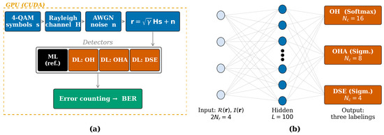
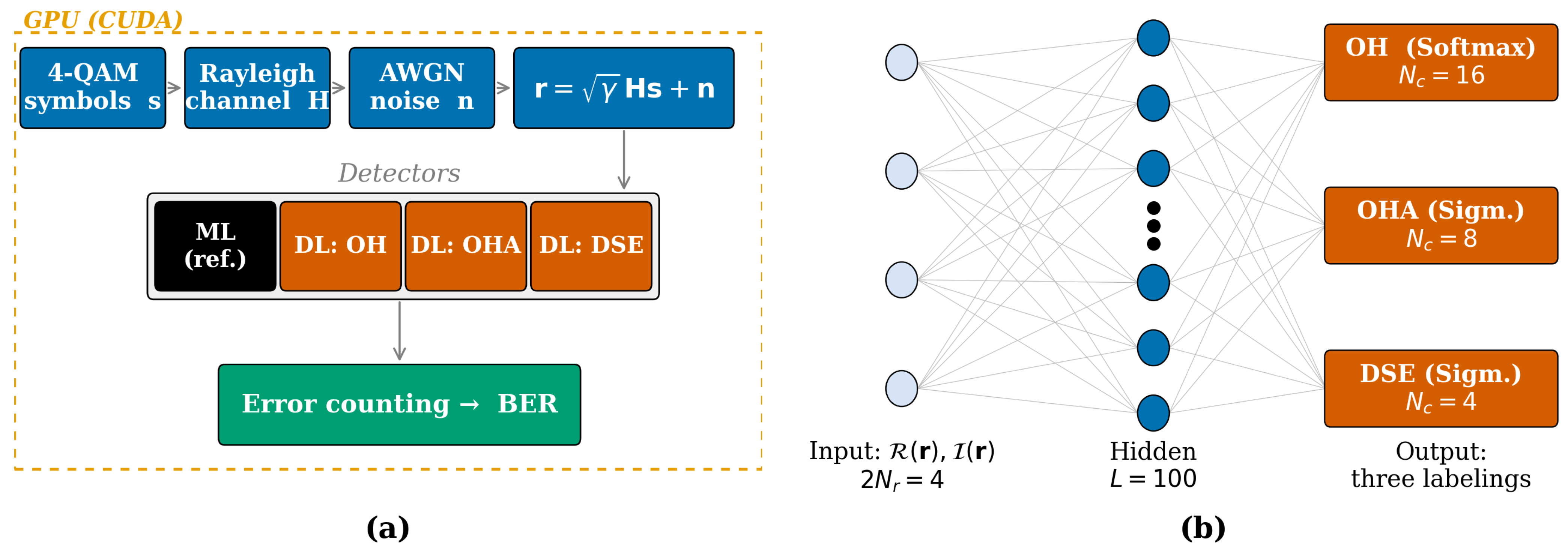
where the output dimension $N_c$ depends on the labeling strategy introduced in Section 2. The concrete values of $N_t$, $N_r$, M, L, and $N_c$ used in this study are specified in Section 4 as part of the simulation scenario. A dense single-hidden-layer network is, in this sense, the minimal sufficient architecture. Its empirical adequacy for $2\times 2$ 4-QAM detection is confirmed in [15], and the universal approximation theorem [7] provides the theoretical basis for why $L=100$ hidden neurons are sufficient for this low-dimensional task. Figure 2 summarizes the complete framework used. Panel (a) depicts the Monte Carlo simulation pipeline and delimits the blocks that execute on GPU; panel (b) details the neural network architecture and the output dimension associated with each of the three labeling strategies.

Figure 2. Evaluated system: (a) Monte Carlo BER pipeline with the GPU (CUDA) blocks boxed; (b) network architecture with three labeling outputs ($N_c=16$ OH, 8 OHA, 4 DSE).

4. Simulation Scenario and Training Framework

4.1. Simulation Scenario

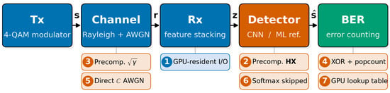
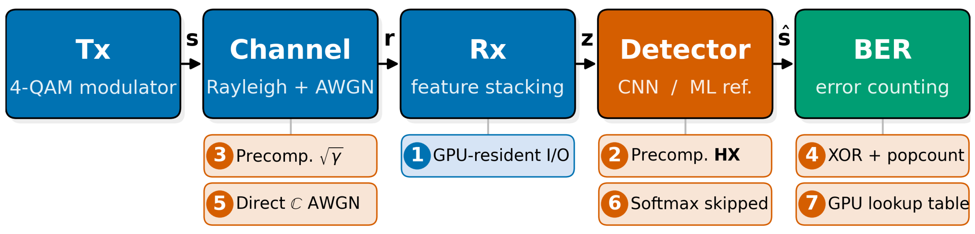
We instantiated a $2\times 2$ MIMO system with 4-QAM modulation ($M=4$, $N_t=N_r=2$) and fixed $L=100$ hidden neurons, consistent with [15,16]. The normalized alphabet was $\mathcal{A}=\{(\pm 1\pm j)/\sqrt{2}\}$. The output dimensions were $N_c=16$ (OH), $N_c=8$ (OHA), and $N_c=4$ (DSE) for the same spectral efficiency. The Monte Carlo simulation used $N_{\mathrm{MC}}={10}^6$ iterations per SNR point over a sweep of $N_{\mathrm{SNR}}=26$ points between 0 and 25 dB, on a fixed quasi-static Rayleigh-fading channel. The computing platform is detailed in Table 2. Figure 3 shows the full communication pipeline and identifies where each optimization is carried out. In this work, the BER was used as a performance metric to compare the systems. The curves were compared when an error rate of 1.0 × ${10}^{-3}$ was reached. Since no encoders have been added, this rate is typically considered sufficient for proper system operation. The difference in SNR needed to reach this rate shows the energy gain of one system compared to the reference system. For fair comparisons, the transmission power remained normalized for all simulations.

Table 2. Hardware and software platform.

Component	Description
GPU	NVIDIA RTX 4090, 24 GB GDDR6X, 16 384 CUDA cores
CPU	Intel Core i9, 24 cores
RAM	32 GB DDR5
Operating sys.	Windows 11
Python	3.11.5
PyTorch	2.5.0+cu121
CUDA Toolkit	12.1
cuDNN	8.9.0

Figure 3. Block diagram of the DL-based 2 × 2 MIMO pipeline; Badges 1 through 7 indicate where each of the seven optimization procedures is carried out.

4.2. Training Configuration

Starting from the reference configuration of [15] (${10}^5$ samples), we evaluated the optimized configuration summarized in Table 3. The number of epochs in the “Base” column (2000) corresponds to the regime used in the initial reproduction of the experiment. The changes aim to increase the effective training capacity without altering the network architecture.

Table 3. Comparison of training configurations.

Parameter	Reference [15]	This Work
Samples	${10}^5$	${10}^6$
Epochs	2000	10,000
Batch mode	Mini-batch	Full batch
Optimizer	SGD ($\mu =0.9$), $\eta =0.01$	SGD ($\mu =0$), $\eta =0.01$
OH output activation	Softmax	Softmax
OHA/DSE output activation	ReLU	Sigmoid
Train/test split	80/20	80/20

The choice of a sigmoid activation at the output layer of OHA and DSE follows the recommendation of [15] for schemes with multiple simultaneously active outputs. This is consistent with the analysis of Glorot, Bordes, and Bengio [35], who showed that saturating nonlinearities at the output are appropriate when several outputs are expected to be simultaneously non-negligible, precisely the case for OHA, where each of the $N_t$ antenna blocks independently activates one of M outputs, and for DSE, where each bit output can independently be zero or one. For the OH scheme, where exactly one of the $M^{N_t}$ classes should dominate, a softmax output trained with cross-entropy yields the required winner-takes-all behavior. Full-batch training at the scale of ${10}^6$ samples is consistent with the large-batch convergence analysis of Bottou [36]; when the loss landscape is well-conditioned, as is typical for shallow networks on low-dimensional, structured inputs such as $\mathbf{x}\in {\mathbb{R}}^{2N_r}$, deterministic gradient descent converges to a tighter neighborhood of the minimum than mini-batch sampling allows. Full-batch is thus a base-configuration choice, practical for this small $2\times 2$ problem whose dataset fits in GPU memory; since the goal of this work is to accelerate the reference experiment rather than to retune its hyperparameters, we do not attribute the BER changes to the batch mode in isolation. Each scheme was trained by minimizing its classification loss (categorical cross-entropy for OH and binary cross-entropy for the per-output OHA and DSE schemes), and the random seeds were fixed for reproducibility. The training metrics used were accuracy and macro F1-score, computed on the test set with scikit-learn [37]. No automated hyperparameter search was used. The reported exploration is a reduction of the configuration space, sufficient to isolate the effect of the activation function and the volume of data on BER performance.

5. Algorithmic Optimization

Evaluating BER performance requires $N_{\mathrm{MC}}\times N_{\mathrm{SNR}}=2.6\times {10}^7$ Monte Carlo iterations, each involving noise generation, channel computation, inference of the three DL detectors, and evaluation of the ML detector. The base pipeline (training with the optimized configuration in Table 3, plus Monte Carlo evaluation without the seven algorithmic optimizations introduced in this section) takes approximately $17.64$ h on the platform of Table 2.

GPU acceleration in this context rests on the CUDA parallel computing model of Nickolls et al. [31], which exposes massive thread-level parallelism to general-purpose workloads. A Monte Carlo BER simulation is naturally data-parallel: the $N_{\mathrm{MC}}$ iterations within each SNR point are mutually independent, and the $N_{\mathrm{SNR}}$ points can be processed in any order. The primary obstacles to full GPU utilization are memory bandwidth, kernel-launch overhead, and redundant host-device data transfers. Algorithm 1 summarizes the optimized end-to-end proposed procedure. The seven optimizations are annotated inline.

Algorithm 1 GPU-accelerated Monte Carlo BER simulation.

Require:  Detector $\mathcal{M}$ (CNN or ML reference); SNR set $\mathcal{S}$ (in dB); iterations N per SNR point; alphabet ${\mathcal{A}}^{N_t}$ (16 entries for 2 × 2 4-QAM); fixed channel $\mathbf{H}$. Ensure:  BER curve $\left\{\mathrm{BER}\right(\gamma ):\gamma \in \mathcal{S}\}$. Pre-computation phase (executed once before the SNR sweep):   1: ${\left\{\sqrt{\gamma }\right\}}_{\gamma \in \mathcal{S}}\leftarrow \left\{\sqrt{{10}^{{\gamma }_{\mathrm{dB}}/10}}\right\}$                                                                    ▹ O3   2: $\mathbf{HX}\leftarrow {\mathcal{A}}^{N_t}{\mathbf{H}}^{\top }$                                                           ▹ O2 (ML baseline)   3: $\mathrm{LUT}[i,j]\leftarrow \mathrm{popcount}(i\oplus j),i,j\in \{0,\dots ,15\}$                         ▹ O7, GPU Main Monte Carlo loop:   4: for each $\gamma \in \mathcal{S}$ do   5:       $E\leftarrow 0$   6:       for $k\leftarrow 1$ to N do   7:             $\mathbf{s}\leftarrow$ random sample of ${\mathcal{A}}^{N_t}$   8:             $\mathbf{n}\leftarrow \mathrm{randn}(N_r,\mathrm{complex}64)$                                                ▹ O5   9:             $\mathbf{r}\leftarrow \sqrt{\gamma }\mathbf{H}\mathbf{s}+\mathbf{n}$ 10:             $\mathbf{z}\leftarrow \mathrm{stack}\left(\Re \left(\mathbf{r}\right),\Im \left(\mathbf{r}\right)\right)$                                 ▹ O1, GPU-resident 11:             $\widehat{i}\leftarrow arg\; max\left(\mathcal{M}\left(\mathbf{z}\right)\right)$                                        ▹ O6, no softmax 12:             $E\leftarrow E+\mathrm{LUT}\left[\mathrm{idx}\left(\mathbf{s}\right),\widehat{i}\right]$                                               ▹ O4, O7 13:       end for 14:       $\mathrm{BER}\left(\gamma \right)\leftarrow E/\left(2N\right)$ 15: end for 16: return$\left\{\mathrm{BER}\right(\gamma ):\gamma \in \mathcal{S}\}$.

5.1. Definition of Time Saving

For each optimization i, we measure the average time $t_i^{\left(b\right)}$ of an isolated operation in the base implementation and $t_i^{\left(o\right)}$ in the optimized one. The relative individual reduction is

$$\Delta T_i=1-{\displaystyle \frac{t_i^{\left(o\right)}}{t_i^{\left(b\right)}}}.$$

(5)

The total saving over the complete simulation is quantified in its end-to-end form:

$$\Delta T_{\mathrm{total}}=1-{\displaystyle \frac{T_{\mathrm{opt}}}{T_{\mathrm{base}}}},$$

(6)

where $T_{\mathrm{base}}$ and $T_{\mathrm{opt}}$ are the end-to-end measured total evaluation times. The corresponding real speedup is $s=T_{\mathrm{base}}/T_{\mathrm{opt}}$.

5.2. Implemented Optimizations

Table 4 summarizes the seven optimizations and the $\Delta T_i$ reduction obtained in each case. Each is briefly described below:

Table 4. Algorithmic optimizations and individual reduction measured via Equation (5).

#	Optimization	$\mathbf{\Delta }{\mathit{T}}_{\mathit{i}}$
1	Elimination of CPU↔GPU transfers	$30\%$
2	Precomputation of $\mathbf{H}\mathbf{s}$ for the ML detector	$10\%$
3	Precomputation of $\sqrt{{\gamma }_j}$ per SNR point	$5\%$
4	Bit-error counting via XOR	$21\%$
5	Direct complex-noise generation	$41\%$
6	Softmax removal at inference	$14\%$
7	Lookup table for bit errors	$38\%$

1.

Elimination of CPU↔GPU transfers. The PCIe 4.0 ×16 interconnect peaks at ∼32 GB/s, roughly 30× lower than the RTX 4090’s on-device GDDR6X bandwidth of ∼1 TB/s. Every tensor assembled on the host and then transferred to GPU uses a bandwidth. The fix is to construct the symbol, channel, and noise tensors directly in device memory via torch.device(‘cuda’), so the only host-device transfer is the BER scalar written at the end of each SNR point. That scalar is four bytes; its transfer cost is negligible.

2.

Precomputation of $\mathbf{H}{\mathbf{s}}_i$ for the ML detector. The ML criterion evaluates $\parallel \mathbf{r}-\sqrt{\gamma }\mathbf{H}{\mathbf{s}}_i{\parallel }^2$ for all $M^{N_t}=16$ candidates ${\mathbf{s}}_i\in {\mathcal{A}}^{N_t}$. Because $\mathbf{H}$ is quasi-static, the products $\mathbf{H}{\mathbf{s}}_i$ are the same for every iteration within a given SNR point. Computing them once and caching the result replaces $16N_{\mathrm{MC}}{N}_{\mathrm{SNR}}=4.16\times {10}^8$ redundant matrix-vector products with 26 precomputed batches of 16.

3.

Precomputation of $\sqrt{{\gamma }_j}$. Straightforward, but measurably useful. Converting 26 SNR values from decibels and extracting square roots inside the inner Monte Carlo loop repeats each operation $N_{\mathrm{MC}}$ times per SNR point for no reason, since $\gamma$ does not change within a point. Moving these 26 scalar computations outside the loop is a one-line change that eliminates $26N_{\mathrm{MC}}$ floating-point instructions per sweep.

4.

Bit-error counting via XOR. The number of differing bits between two symbol indices a and b is $\mathrm{popcount}(a\oplus b)$, where ⊕ is bitwise XOR. GPUs implement popcount in a single hardware instruction [38]. Casting symbol indices to integers and issuing a batched XOR + popcount reduces $N_{\mathrm{MC}}$ sequential comparison loops to one vectorized GPU kernel call, with the same result at a fraction of the instruction count.

5.

Direct generation of complex noise. The base implementation draws real and imaginary AWGN components with two separate torch.randn calls, each triggering an independent CUDA kernel launch. The PyTorch complex64 dtype consolidates both into one call, halving kernel-launch overhead for noise generation across $N_{\mathrm{MC}}\times N_{\mathrm{SNR}}=2.6\times {10}^7$ iterations.

6.

Elimination of softmax at inference. $arg\; max\left(\mathrm{softmax}\right(\mathbf{z}\left)\right)=arg\; max\left(\mathbf{z}\right)$ for any $\mathbf{z}$: the monotone normalization cannot change which element wins. Removing it at the decision stage eliminates one full pass over each $N_c$-dimensional output. Across the complete simulation (three labeling strategies, $N_{\mathrm{MC}}$ iterations, $N_{\mathrm{SNR}}$ points), this removes ∼$7.8\times {10}^7$ softmax evaluations without touching the BER numbers.

7.

Lookup table for bit errors. Converting a class index $i\in \{0,\dots ,15\}$ to a four-bit symbol normally requires modulus and right-shift operations per bit. A $16\times 16$ popcount table, precomputed once on GPU and indexed by $(\mathrm{idx}\left(\mathbf{s}\right),\widehat{i})$, replaces all of that arithmetic with a single coalesced read. The table is 256 bytes and fits in L1 cache (∼128 KB per SM on the RTX 4090), so $N_{\mathrm{MC}}$ repeated lookups over a single SNR point incur no cache-miss penalty after the first access.

5.3. Measurement Methodology

Each optimization is evaluated independently using torch.cuda.Event, averaging $10,000$ cycles per configuration with 100 preliminary iterations. For the end-to-end measurement, the full Monte Carlo simulation is run on the platform of Table 2, synchronizing with torch.cuda.synchronize() at the beginning and end of the SNR sweep. This measurement is reported as wall-clock time and used in Equation (6).

5.4. Multiplicative Ceiling vs. Real Speedup

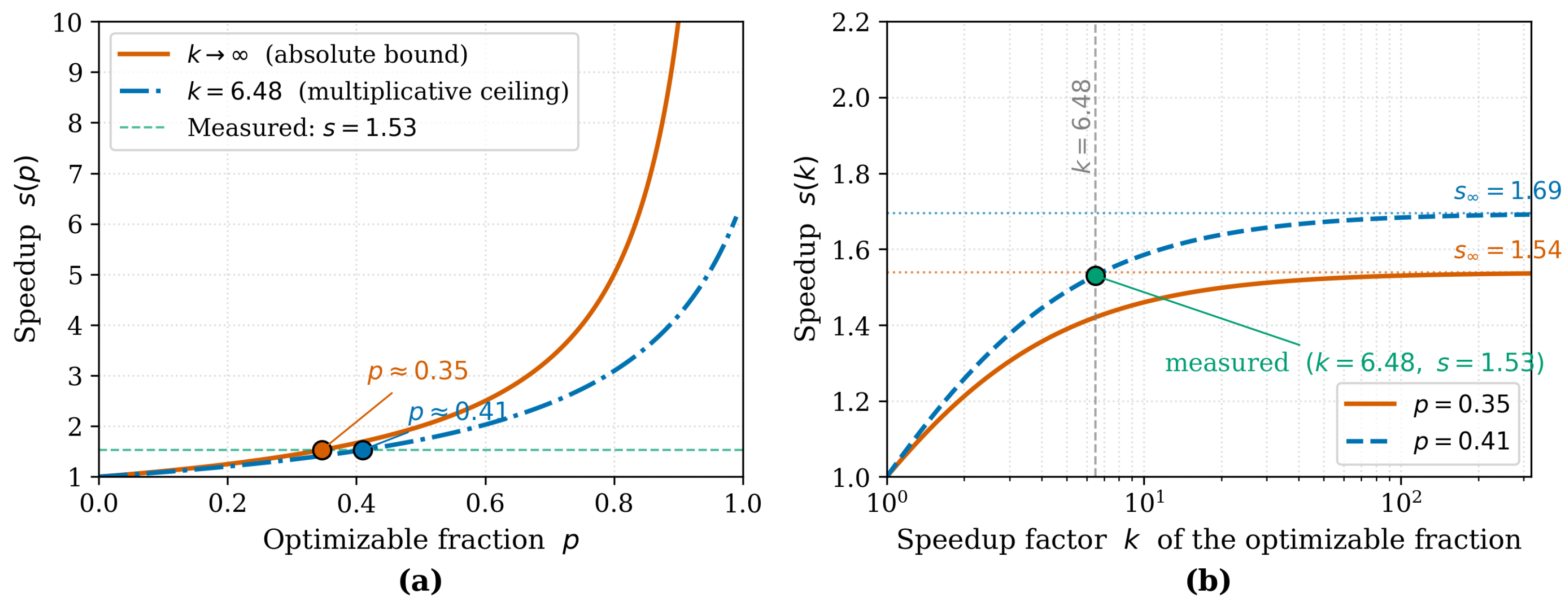
The theoretical speedup for a multiplicative optimization would be ${\prod }_{i}1/(1-\Delta T_i)\approx 6.48\times$, a figure computed with the $\Delta T_i$ at the full precision recorded by torch.cuda.Event. This result differs slightly from the product that results from the integer percentages shown in Table 4. The measured real speedup, $s=17.64/11.51\approx 1.53\times$, falls noticeably below. Amdahl’s law [18] offers a direct reading of this gap: if only a fraction p of the total time is parallelizable or optimizable, the net speedup is bounded by $s\le 1/(1-p)$. A value $s\approx 1.53$ is consistent with an optimizable fraction on the order of $p\approx 0.35$ (a lower bound under the asymptotic approximation $k\to \infty$) or $p\approx 0.41$ if the individual ceiling is taken to be $6.48\times$. Under either reading, training dominates a substantial portion of the pipeline, and these optimizations do not affect it directly.

Figure 4 shows this discussion. Figure 4a shows the speedup s as a function of the optimizable fraction p under both readings ($k\to \infty$ and $k=6.48$), with the measured operating point $(p,s)$ highlighted. Figure 4b fixes p and varies the individual ceiling k: the curve saturates rapidly, evidencing that, beyond a certain point, increasing k yields marginal gains unless p grows alongside.

Figure 4. Amdahl’s law: (a) speedup s vs. optimizable fraction p for $k\to \infty$ and $k=6.48$, with operating point $(0.41,1.53)$; (b) s vs. ceiling k at fixed p.

6. Results and Discussion

6.1. Training Performance

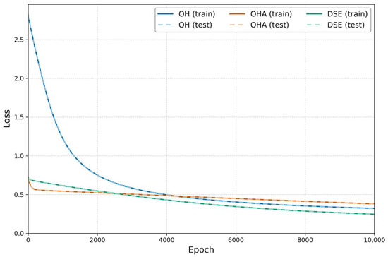
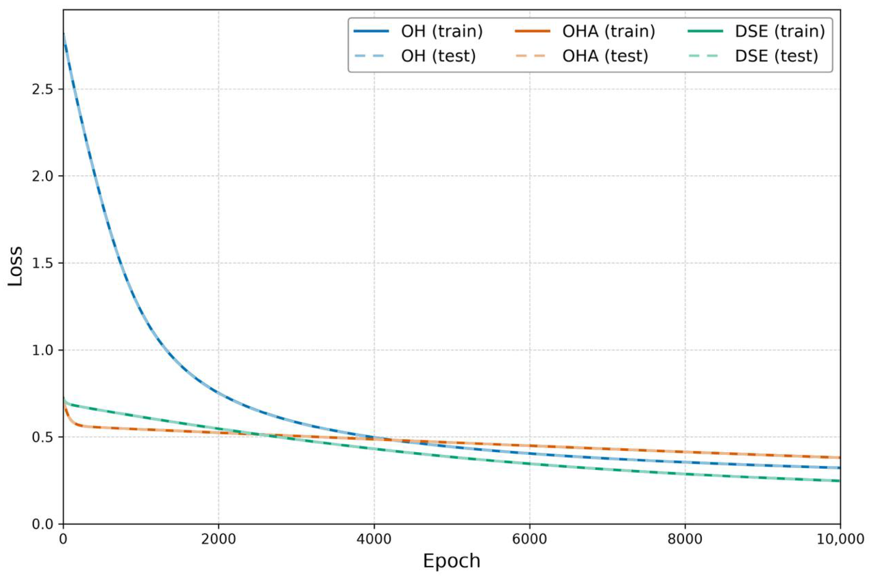
Table 5 summarizes the classification metrics obtained with the optimized configuration. The OH scheme reaches an accuracy of $91.39\%$ with 16 outputs; OHA and DSE operate with fewer outputs (eight and four, respectively) at the cost of slightly lower accuracy (∼86.5%). Figure 5 shows the training and test loss for the three schemes over the 10,000 epochs. For every scheme the test loss tracks the training loss throughout and reaches its minimum at the final epoch (the final gap between training and test loss is below ${10}^{-3}$), and the test accuracy matches the training accuracy to within 0.05 percentage points; there is therefore no evidence of overfitting, even at this extended training budget. This is consistent with the absence of overfitting reported for the same architecture in [15].

Table 5. Training metrics with the optimized configuration.

Scheme	Outputs	Accuracy	F1-Score
One-Hot	16	$91.39\%$	$0.9141$
One-Hot-per-Antenna	8	$86.59\%$	$0.8663$
Direct Symbol Encoding	4	$86.50\%$	$0.8654$

Figure 5. Training (solid) and test (dashed) loss over the 10,000 epochs for the three labeling schemes (OH, OHA, DSE); the test loss overlaps the training loss, indicating no overfitting.

6.2. BER Performance

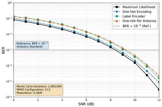
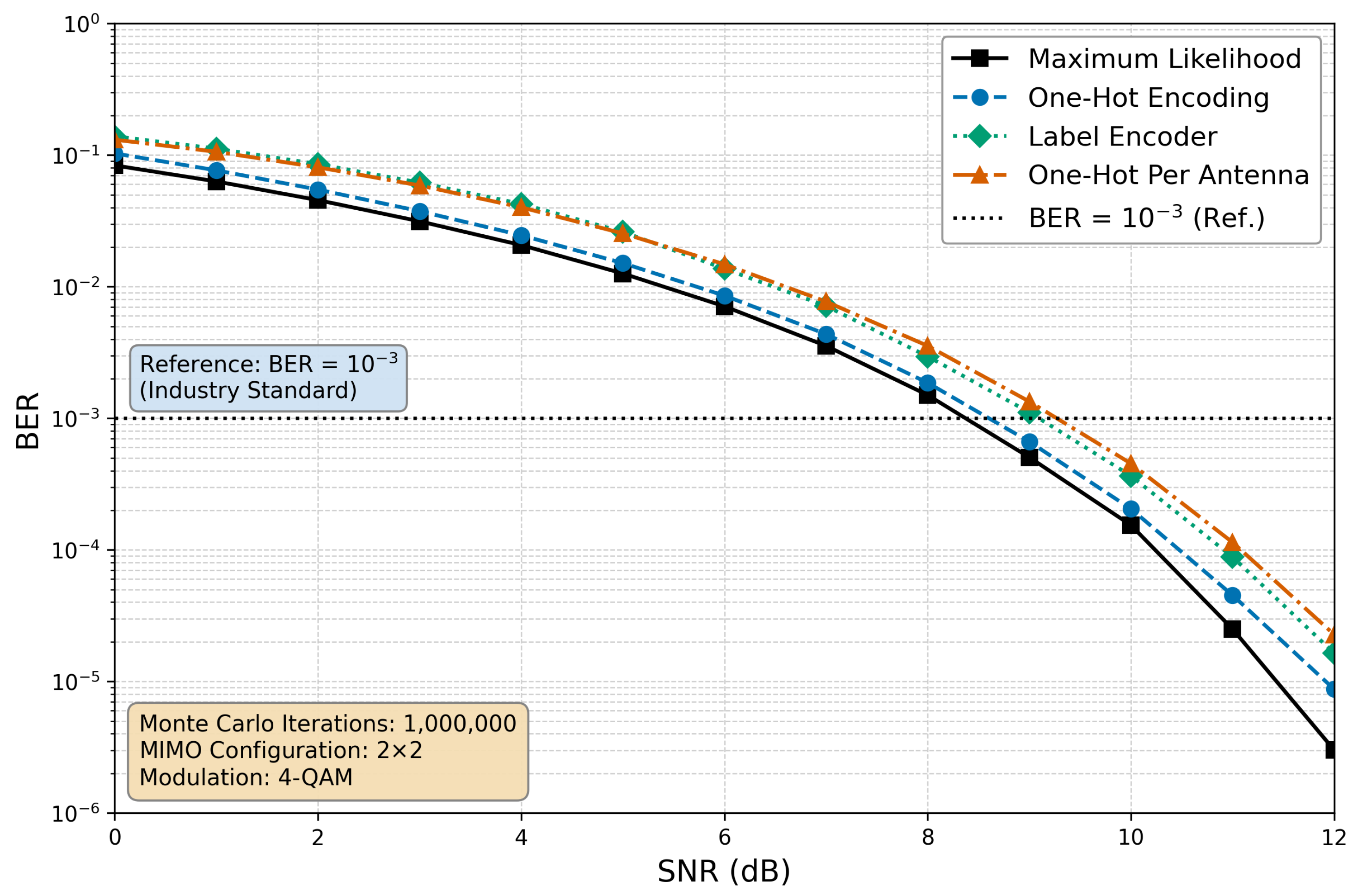
Figure 6 shows the BER curves as a function of SNR for the four detectors: ML (optimal reference), OH, OHA, and DSE. In all cases, curves were obtained with ${10}^6$ Monte Carlo iterations per SNR point in the 0–25 dB range on the fixed quasi-static channel.

Figure 6. BER curves vs. SNR for the $2\times 2$ MIMO system with 4-QAM, optimized training configuration.

To quantify proximity to the optimal detector, we define the gap as the horizontal distance, in decibels, between the evaluated detector’s curve and the ML curve at the BER $={10}^{-3}$ crossing. Table 6 summarizes the gaps obtained for the base and optimized configurations.

Table 6. BER performance at ${10}^{-3}$: base vs. optimized configuration.

	Gap vs. ML (dB)
Detector	Base [15]	This Work	$\mathbf{\Delta }$ Gap (dB)
ML (reference)	$0.00$	$0.00$	n/a
One-Hot	$1.00$	∼$0.20$	$-0.80$
One-Hot-per-Antenna	$2.00$	∼$0.90$	$-1.10$
Direct Symbol Encoding	$0.30$	∼$0.70$	$+0.40$

Negative $\Delta$ gap values indicate a reduction of the distance to the ML detector (improvement); positive values indicate regression.

The optimized configuration substantially improves OH and OHA. For OH, the gap drops from 1.00 dB to ∼0.20 dB, an improvement that can be attributed mainly to the tenfold increase in training-data volume. OHA improves from 2.00 dB to ∼0.90 dB, confirming Sigmoid as the appropriate activation function for schemes with multiple simultaneously active outputs. DSE, in contrast, decreases slightly under Sigmoid, which suggests that for this scheme, ReLU remains preferable under backpropagation training.

Below 5 dB, all three DL detectors look equally poor, as expected. The received energy per symbol is insufficient for any labeling strategy to separate the 4-QAM constellation symbols. In this case, BER approaches 0.5 across the board. The informative range is roughly 10–20 dB, where the three schemes diverge. OH maps the entire transmitted pair to a single class out of $M^{N_t}=16$, giving the network the most complete target: one probability vector encoding the joint distribution of both transmitted symbols. OHA splits that joint decision into two independent per-antenna problems, while DSE further compresses to raw bit outputs. Therefore, DSE is most sensitive to the activation choice at the output layer; the $+0.40$ dB regression under Sigmoid in Table 6 is not an anomaly. It follows from the fact that DSE’s four binary outputs are expected to be sparse, and Sigmoid is not adequate for sparse activation.

All data in this work are fully synthetic, obtained from simulated channel realizations; each reported BER is therefore a Monte Carlo estimate rather than a closed-form expression, and a brief note on its statistical reliability is in order. Every point aggregates $N_b=N_{\mathrm{MC}}{log}_2\left(M\right)N_t=4\times {10}^6$ transmitted bits, so the estimator is binomial and admits the normal-approximation 95% confidence interval $\widehat{\mathrm{BER}}\pm 1.96\sqrt{\widehat{\mathrm{BER}}(1-\widehat{\mathrm{BER}})/N_b}$. To keep that interval meaningful at low error rates, the simulation requires at least 100 counted bit errors per SNR point (the conventional threshold for a $\pm 20\%$ interval at 95% confidence in communication-system Monte Carlo studies [39]), and the SNR sweep is halted once no detector reaches this count, so that no unreliable point is reported. At the $\mathrm{BER}={10}^{-3}$ level where the gaps in Table 6 are read, this corresponds to roughly 4000 errors and a relative confidence interval of about $\pm 3\%$, tightening to near $\pm 1\%$ around ${10}^{-2}$. Since the OH, OHA, and DSE curves are separated by far more than this margin throughout the informative SNR range, the reported ordering and the resulting BER gaps reflect genuine differences between the labeling schemes rather than finite-sample noise.

6.3. Compute Gains

The wall-clock time for a full evaluation, measured in accordance with Section 5.3, drops from $T_{\mathrm{base}}=17.64$ h in the base implementation to $T_{\mathrm{opt}}=11.51$ h in the optimized implementation, a saving of 6.12 h per complete simulation (34.7%, $1.53\times$). This value falls below the $6.48\times$ multiplicative ceiling implied by the individual reductions in Table 4 and is attributable to the non-optimizable fraction of the pipeline (chiefly the training stages).

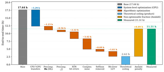
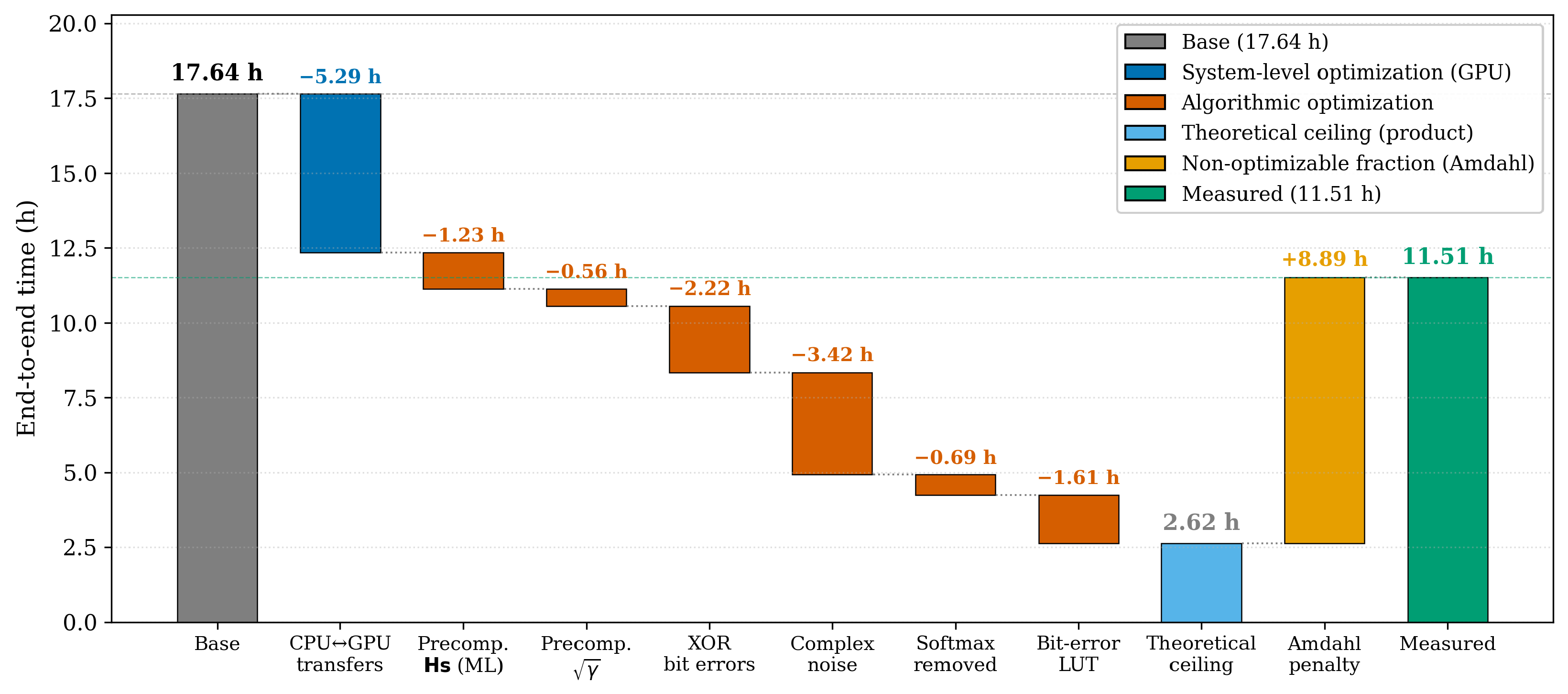
Figure 7 illustrates these results. Note that if each optimization operated under a strictly multiplicative regime and covered the entire pipeline, the successive application of the seven reductions would bring the total time from 17.64 h down to approximately 2.72 h. The gap between that theoretical ceiling and the actual achieved time (11.51 h) is rendered as the Amdahl penalty.

Figure 7. End-to-end runtime cascade: the successive $\Delta T_i$ of Table 4 reduce $T_{\mathrm{base}}=17.64$ h; the gap to the measured $11.51$ h is the Amdahl penalty (net saving 6.12 h, $34.7\%$).

7. Conclusions

In this work, a CUDA-enabled PyTorch implementation and an improvement of the DL-based MIMO detection scheme reported in [15] have been presented. On the training side, the optimized configuration shrinks the gap with the ML detector from 1.00 dB to ∼0.20 dB for the OH labeling and from 2.00 dB to ∼0.90 dB for the OHA labeling. Sigmoid activation is confirmed to be appropriate for OHA but not for DSE under backpropagation. On the simulation, seven algorithmic optimizations reduced the complete evaluation from 17.64 h to 11.51 h on an NVIDIA RTX 4090, a saving of 6.12 h (34.7%, $1.53\times$). Also, the gap between this real speedup and the multiplicative ceiling of $6.48\times$ admits a direct explanation in Amdahl’s law. As future work, it is of interest to extend the study to larger MIMO configurations and higher-order modulations, where the attainable acceleration ceiling is potentially larger, as well as to evaluate the impact of training with a random channel instead of a semi-static channel.

References

- Foschini, G.J.; Gans, M.J. On Limits of Wireless Communications in a Fading Environment when Using Multiple Antennas. Wirel. Pers. Commun. 1998, 6, 311–335. [Google Scholar] [CrossRef] [Scilit]
- Telatar, E. Capacity of Multi-Antenna Gaussian Channels. Eur. Trans. Telecommun. 1999, 10, 585–595. [Google Scholar] [CrossRef] [Scilit]
- Marzetta, T.L. Noncooperative Cellular Wireless with Unlimited Numbers of Base Station Antennas. IEEE Trans. Wirel. Commun. 2010, 9, 3590–3600. [Google Scholar] [CrossRef] [Scilit]
- Viterbo, E.; Boutros, J. A Universal Lattice Code Decoder for Fading Channels. IEEE Trans. Inf. Theory 1999, 45, 1639–1642. [Google Scholar] [CrossRef] [Scilit]
- Hassibi, B.; Vikalo, H. On the Sphere-Decoding Algorithm I: Expected Complexity. IEEE Trans. Signal Process. 2005, 53, 2806–2818. [Google Scholar] [CrossRef] [Scilit]
- LeCun, Y.; Bengio, Y.; Hinton, G. Deep Learning. Nature 2015, 521, 436–444. [Google Scholar] [CrossRef] [Scilit] [PubMed]
- Goodfellow, I.; Bengio, Y.; Courville, A. Deep Learning; MIT Press: Cambridge, MA, USA, 2016. [Google Scholar]
- O’Shea, T.J.; Hoydis, J. An Introduction to Deep Learning for the Physical Layer. IEEE Trans. Cogn. Commun. Netw. 2017, 3, 563–575. [Google Scholar] [CrossRef] [Scilit]
- Ye, H.; Li, G.Y.; Juang, B.H. Power of Deep Learning for Channel Estimation and Signal Detection in OFDM Systems. IEEE Wirel. Commun. Lett. 2018, 7, 114–117. [Google Scholar] [CrossRef] [Scilit]
- Keawin, C.; Innok, A.; Uthansakul, P. Optimization of Signal Detection Using Deep CNN in Ultra-Massive MIMO. Telecom 2024, 5, 280–295. [Google Scholar] [CrossRef] [Scilit]
- Mawlood, M.A.; Mahmood, D.A. Optimizing Weighted Fair Queuing with Deep Reinforcement Learning for Dynamic Bandwidth Allocation. Telecom 2025, 6, 46. [Google Scholar] [CrossRef] [Scilit]
- Samuel, N.; Diskin, T.; Wiesel, A. Learning to Detect. IEEE Trans. Signal Process. 2019, 67, 2554–2564. [Google Scholar] [CrossRef] [Scilit]
- Khani, M.; Alizadeh, M.; Hoydis, J.; Fleming, P. Adaptive Neural Signal Detection for Massive MIMO. IEEE Trans. Wirel. Commun. 2020, 19, 5635–5648. [Google Scholar] [CrossRef] [Scilit]
- He, H.; Wen, C.K.; Jin, S.; Li, G.Y. Model-Driven Deep Learning for MIMO Detection. IEEE Trans. Signal Process. 2020, 68, 1702–1715. [Google Scholar] [CrossRef] [Scilit]
- Ibarra-Hernández, R.F.; Castillo-Soria, F.R.; Gutiérrez, C.A.; Del-Puerto-Flores, J.A.; Acosta-Elias, J.; Rodriguez-Abdala, V.I.; Palacios-Luengas, L. Efficient Deep Learning-Based Detection Scheme for MIMO Communication Systems. Sensors 2025, 25, 669. [Google Scholar] [CrossRef] [Scilit] [PubMed]
- Ibarra-Hernández, R.F.; Castillo-Soria, F.R.; Zabala-Blanco, D.; Datta, J.; Castro-Tapia, S.; Ibarra-Delgado, S. BER Performance Comparison of ELM Signal Detection Schemes for MIMO Channels. In Proceedings of the 2025 IEEE Latin-American Conference on Communications (LATINCOM), Antigua, Guatemala, 5–7 November 2025; pp. 1–6. [Google Scholar]
- Paszke, A.; Gross, S.; Massa, F.; Lerer, A.; Bradbury, J.; Chanan, G.; Killeen, T.; Lin, Z.; Gimelshein, N.; Antiga, L.; et al. PyTorch: An Imperative Style, High-Performance Deep Learning Library. In Proceedings of the Advances in Neural Information Processing Systems 32 (NeurIPS), Vancouver, BC, Canada, 8–14 December 2019; pp. 8024–8035. [Google Scholar]
- Amdahl, G.M. Validity of the Single Processor Approach to Achieving Large Scale Computing Capabilities. In Proceedings of the Spring Joint Computer Conference (AFIPS ’67), Atlantic City, NJ, USA, 18–20 April 1967; pp. 483–485. [Google Scholar] [CrossRef] [Scilit]
- Goldsmith, A. Wireless Communications; Cambridge University Press: Cambridge, UK, 2005. [Google Scholar]
- Tse, D.; Viswanath, P. Fundamentals of Wireless Communication; Cambridge University Press: Cambridge, UK, 2005. [Google Scholar]
- Balatsoukas-Stimming, A.; Studer, C. Deep Unfolding for Communications Systems: A Survey and Some New Directions. In Proceedings of the IEEE International Workshop on Signal Processing Systems (SiPS), Nanjing, China, 20–23 October 2019; pp. 266–271. [Google Scholar] [CrossRef] [Scilit]
- Gao, J.; Chen, X.; Li, G.Y. Deep Unfolding Based Channel Estimation for Wideband Terahertz Near-Field Massive MIMO Systems. Front. Inf. Technol. Electron. Eng. 2024, 25, 1162–1172. [Google Scholar] [CrossRef] [Scilit]
- Daha, M.Y.; Sudhakaran, A.; Babu, B.; Hadi, M.U. Enabling Intelligent 6G Communications: A Scalable Deep Learning Framework for MIMO Detection. Telecom 2025, 6, 58. [Google Scholar] [CrossRef] [Scilit]
- Omondi, G.; Olwal, T.O. A DNN-Based MIMO Signal Detector Using Transformer Architecture for Next-Generation Wireless Networks. J. Inf. Intell. 2025, 3, 526–546. [Google Scholar] [CrossRef] [Scilit]
- Ye, H.; Liang, L. On Purely Data-Driven Massive MIMO Detectors. IEEE Trans. Signal Process. 2025, 73, 3079–3093. [Google Scholar] [CrossRef] [Scilit]
- Sejan, M.A.S.; Rahman, M.H.; Song, H.K. Demod-CNN: A Robust Deep Learning Approach for Intelligent Reflecting Surface-Assisted Multiuser MIMO Communication. Sensors 2022, 22, 5971. [Google Scholar] [CrossRef] [Scilit] [PubMed]
- Rahman, M.H.; Sejan, M.A.S.; Aziz, M.A.; Kim, D.S.; You, Y.H.; Song, H.K. Deep Convolutional and Recurrent Neural-Network-Based Optimal Decoding for RIS-Assisted MIMO Communication. Mathematics 2023, 11, 3397. [Google Scholar] [CrossRef] [Scilit]
- Ranjan, A.; Sahana, B.C. Deep Learning Empowered Channel Estimation in Massive MIMO: Unveiling the Efficiency of Hybrid Deep Learning Architecture. J. Ambient. Intell. Humaniz. Comput. 2025, 16, 375–390. [Google Scholar] [CrossRef] [Scilit]
- Tian, X.; Zheng, Q. A Massive MIMO Channel Estimation Method Based on Hybrid Deep Learning Model with Regularization Techniques. Int. J. Intell. Syst. 2025, 2025, 2597866. [Google Scholar] [CrossRef] [Scilit]
- Kumar, A.; Gaur, N.; Nanthaamornphong, A. Machine Learning RNNs, SVM and NN Algorithm for Massive-MIMO-OTFS 6G Waveform with Rician and Rayleigh Channel. Egypt. Inform. J. 2024, 27, 100531. [Google Scholar] [CrossRef] [Scilit]
- Nickolls, J.; Buck, I.; Garland, M.; Skadron, K. Scalable Parallel Programming with CUDA. ACM Queue 2008, 6, 40–53. [Google Scholar] [CrossRef] [Scilit]
- Liao, Y.; Shangguan, M.; Yang, Z.; Lin, Z.; Wang, Y.; Li, S. GPU-Accelerated Monte Carlo Simulation for a Single-Photon Underwater Lidar. Remote Sens. 2023, 15, 5245. [Google Scholar] [CrossRef] [Scilit]
- Yu, C.; Kim, D.; Lee, H.; Han, M. GPU-Accelerated CNN Inference for Onboard DQN-Based Routing in Dynamic LEO Satellite Networks. Aerospace 2024, 11, 1028. [Google Scholar] [CrossRef] [Scilit]
- Baek, M.S.; Kwak, S.; Jung, J.Y.; Kim, H.M.; Choi, D.J. Implementation Methodologies of Deep Learning-Based Signal Detection for Conventional MIMO Transmitters. IEEE Trans. Broadcast. 2019, 65, 636–642. [Google Scholar] [CrossRef] [Scilit]
- Glorot, X.; Bordes, A.; Bengio, Y. Deep Sparse Rectifier Neural Networks. PMLR Workshop Conf. Proc. 2011, 15, 315–323. [Google Scholar]
- Bottou, L. Large-Scale Machine Learning with Stochastic Gradient Descent. In Proceedings of the 19th International Conference on Computational Statistics (COMPSTAT), Paris, France, 22–27 August 2010; pp. 177–186. [Google Scholar] [CrossRef] [Scilit]
- Pedregosa, F.; Varoquaux, G.; Gramfort, A.; Michel, V.; Thirion, B.; Grisel, O.; Blondel, M.; Prettenhofer, P.; Weiss, R.; Dubourg, V.; et al. Scikit-learn: Machine Learning in Python. J. Mach. Learn. Res. 2011, 12, 2825–2830. [Google Scholar]
- Harris, C.R.; Millman, K.J.; van der Walt, S.J.; Gommers, R.; Virtanen, P.; Cournapeau, D.; Wieser, E.; Taylor, J.; Berg, S.; Smith, N.J.; et al. Array Programming with NumPy. Nature 2020, 585, 357–362. [Google Scholar] [CrossRef] [Scilit] [PubMed]
- Jeruchim, M.C.; Balaban, P.; Shanmugan, K.S. Simulation of Communication Systems: Modeling, Methodology, and Techniques, 2nd ed.; Kluwer Academic/Plenum Publishers: New York, NY, USA, 2000. [Google Scholar]
Disclaimer/Publisher’s Note: The statements, opinions and data contained in all publications are solely those of the individual author(s) and contributor(s) and not of MDPI and/or the editor(s). MDPI and/or the editor(s) disclaim responsibility for any injury to people or property resulting from any ideas, methods, instructions or products referred to in the content. |
© 2026 by the authors. Licensee MDPI, Basel, Switzerland. This article is an open access article distributed under the terms and conditions of the Creative Commons Attribution (CC BY) license.