Resource-Constrained Adaptive Sampling for Variance Monitoring: Comparing Rule-Based, MLP, and LSTM Acquisition Policies

Abstract

Automated monitoring must balance detection delay and measurement use. This study compares rule-based, feedforward multilayer perceptron (MLP), and long short-term memory (LSTM) acquisition policies coupled to a common exponentially weighted moving average (EWMA) variance detector. Experiments 1 and 2 comprise 714,000 and 660,000 test trajectories, respectively. Closely matched rule and LSTM configurations achieve in-control average run lengths of 369.97 and 370.11, consumption of 4.918 and 4.917 observations per epoch, and weighted detection delays of 18.860 and 18.864 epochs; the conditional 95% bootstrap confidence interval for the difference in their weighted delays includes zero. A third experiment repeats optimization, selection, calibration, and testing ten times per family, comparing a search budget of 512 candidate evaluations with one of 30 CPU seconds. The mean LSTM-minus-rule delay contrasts are −0.219 and +0.206 epochs, respectively, with across-run 95% intervals [−0.723, 0.285] and [−0.295, 0.708]. Scenario weights, measurement prices, and acquisition duration further affect policy comparisons. The findings characterize the evaluated finite search procedures and operating points within a common detector; they establish neither intrinsic superiority nor equivalence of the policy architectures.

1. Introduction

Automated inspection systems make two related decisions: whether the available evidence indicates a process change, and how much additional information should be acquired. A fixed sampling plan simplifies operation, but it uses the same number of measurements when a process appears stable and when the evidence approaches an alarm threshold. Adaptive acquisition can redistribute this effort. Its value must therefore be assessed jointly through detection delay, false-alarm behavior, and measurement consumption.

Variable sample size control is an established idea. Costa [1] studied a mean chart in which the next sample size depends on the preceding observation. For dispersion monitoring, Castagliola [2] developed an $S^2$-EWMA chart, while Haq [3] adapted the EWMA smoothing parameter using an estimated dispersion shift. These approaches act on different components of a monitoring scheme: the sampling plan, the transformation of dispersion information, and the accumulation of evidence. They should not be treated as interchangeable implementations of a single adaptive method.

Recent studies make the distinction particularly relevant. Abbasi and Noor-ul-Amin [4] investigated adaptive sample size strategies for dispersion monitoring using a quadratic sigmoid EWMA construction. Ahmadini et al. [5] studied a variable sample size EWMA design formulated for the coefficient of variation. Thus, neither adaptive dispersion monitoring nor the combination of EWMA and variable sampling constitutes a new contribution by itself. The latter study also illustrates why the monitored parameter must be specified carefully: a coefficient-of-variation change and a variance change under a known reference distribution define different statistical problems.

Repetitive sampling provides another mechanism for increasing information when the first sample is inconclusive. Aslam et al. [6] introduced an $S^2$ chart with inner and outer limits using repetitive sampling. The present study instead limits acquisition to one additional subgroup within an epoch and retains the EWMA state across epochs. Consequently, the number of epochs until an alarm differs from the number of subgroups and from the number of individual measurements. Reporting only one of these quantities can conceal the operational price of faster detection.

Machine learning adds a further design choice. Tran et al. [7] surveyed applications of learning methods to control-chart design, pattern recognition, and interpretation. Qiu et al. [8] developed predictive monitoring based on LSTM prediction intervals for data with time-varying variability. Their prediction-based setting differs from the present use of recurrent states to allocate measurements while a conventional EWMA statistic determines the alarm. Evidence that recurrent prediction works in temporally structured data does not establish that recurrent acquisition will improve monitoring of independent observations after a permanent variance change.

Learning-based statistical process control (SPC) also includes tasks other than acquisition control. Zan et al. [9] used bidirectional LSTM feature learning for histogram and control-chart pattern recognition. Chiu and Fu [10] investigated the recognition of mixture control-chart patterns in autocorrelated processes using a hybrid convolutional neural network (CNN)–LSTM model. Suárez Castro and Ladino Vega [11] trained an LSTM to approximate EWMA values in individual temperature measurements. These studies concern recognition or prediction from available data. The present comparison concerns the decision to acquire those data, with a separate EWMA alarm rule. Classification or prediction performance therefore cannot be taken as evidence of an acquisition-policy advantage.

The problem also connects to sequential decision-making with observation costs. Banerjee and Veeravalli [12] studied on–off observation control in a Bayesian change-detection formulation, while Nitinawarat and Veeravalli [13] considered controlled sensing with nonuniform acquisition costs. These works show why observation allocation belongs in the monitoring objective. Their risk criteria and observation models differ from the present variance-monitoring experiment, so their optimality results are not transferred to this design.

This study contributes a causal and reproducible framework for comparing acquisition policies under explicit resource constraints. The framework combines predictable subgroup sizes and bounded resampling with a common EWMA variance detector, states the conditional in-control score law, and fixes the acquisition action space for the comparison. Rule-based, feedforward MLP, and recurrent LSTM policies are evaluated under a common resource ceiling, including a closely matched in-control comparison of selected rule-based and LSTM policies. Experiment 1 examines acquisition adaptation and the effect of removing resampling, while Experiment 2 assesses optimization-budget sensitivity and a feedforward policy with the same inputs through independent calibration and testing. Experiment 3 uses ten independent optimization chains per family, separate candidate and computation budgets, and repeated selection, calibration, and final testing to quantify variability across complete procedures. Detection delay in epochs is assessed jointly with individual measurement use and sensitivity to hypothetical measurement prices and acquisition duration. Together, these analyses examine whether the tested recurrent representation adds measurable value and how operational assumptions affect policy choice. The contribution concerns methodological comparison within the specified experimental framework and does not establish superiority over published adaptive dispersion charts.

2. Monitoring Model and Performance Criteria

2.1. Observation Model and Information Ordering

Let $X_{tji}$ denote observation i in subgroup j of epoch t. At most, two subgroups can be acquired in an epoch. Observations are independent and normally distributed with a constant mean and the following time-dependent variance:

$${\sigma }_t^2=\left\{\begin{array}{cc}{\sigma }_0^2,\hfill & t<\tau ,\hfill \\ c{\sigma }_0^2,\hfill & t\ge \tau ,\hfill \end{array}\right.c\ge 1,$$

(1)

where ${\sigma }_0^2$ is known and $\tau$ is the change epoch. Throughout this paper, c is a ratio of variances, not standard deviations. The simulations use ${\sigma }_0^2=1$ without loss of generality with respect to scale. This is a Phase II monitoring experiment; uncertainty from estimating the reference variance is outside its scope.

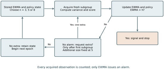
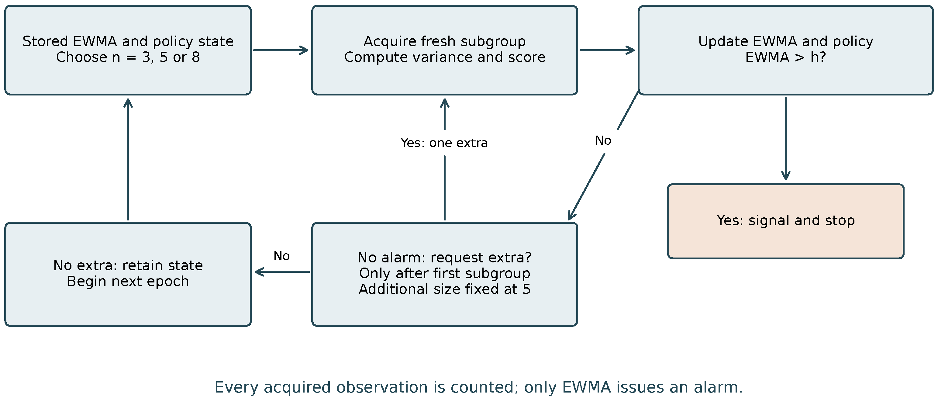
The initial subgroup size $n_{t1}\in \{3,5,8\}$ is chosen from the information available before epoch t. After observing that subgroup, the detector and policy state are updated. If no alarm occurs, the policy can request one additional subgroup of size $n_{t2}=5$. That decision is made before the second subgroup is observed. The additional subgroup is not pooled with the first: each sample variance separately updates the detector. All measurements enter the cost calculation. A non-signaling epoch ends after its first or second subgroup, and the state is retained. Figure 1 summarizes this acquisition sequence and its connection to the detector.

Figure 1. Causal acquisition and detection framework. The request for an additional subgroup is made after the first update and before acquiring new data. Both acquisitions count toward observation use.

2.2. Normal-Score EWMA Detector

For each acquired subgroup, define

$$S_{tj}^2={\displaystyle \frac{1}{n_{tj}-1}}{\displaystyle \sum _{i=1}^{n_{tj}}}{(X_{tji}-{\overline{X}}_{tj})}^2,Q_{tj}={\displaystyle \frac{(n_{tj}-1)S_{tj}^2}{{\sigma }_0^2}}.$$

(2)

Conditional on the predictably selected subgroup size, $Q_{tj}/c$ has a chi-square distribution with $n_{tj}-1$ degrees of freedom after the change. The input to the detector is

$$Z_{tj}={\mathrm{\Phi }}^{-1}\left[F_{{\chi }_{n_{tj}-1}^2}\left(Q_{tj}\right)\right],$$

(3)

where $\mathrm{\Phi }$ denotes the standard normal distribution function. Numerically, the probability is clipped to $[{10}^{-10},1-{10}^{-10}]$ before inversion.

Index acquired subgroups by k, regardless of epoch. The detector updates as

$$E_k=(1-\lambda )E_{k-1}+\lambda Z_k,E_0=0,\lambda =0.1,$$

(4)

and signals immediately when $E_k>h$. The same recursion is used in all configurations; each configuration receives its own calibrated h.

Proposition 1

(Conditional innovation invariance). Let ${\mathcal{F}}_{k-1}$ contain all information available before acquisition k, including internal policy states and any independent policy randomization. Assume a known ${\sigma }_0^2$, an ${\mathcal{F}}_{k-1}$-measurable integer $n_k\ge 2$, and fresh independent normal observations with variance ${\sigma }_0^2$ conditional on that information. Ignoring numerical clipping, each newly acquired normal score in Equation (3) satisfies $Pr(Z_k\le z\mid {\mathcal{F}}_{k-1})=\mathrm{\Phi }\left(z\right)$. In particular, without within-epoch resampling, a predictable sample-size policy does not change the in-control run-length distribution of the normal-score EWMA with a fixed common limit.

Proof. 

Conditional on the past, the selected subgroup size is known and the fresh observations are independent of that past. The conditional distribution of Q is therefore ${\chi }_{n-1}^2$. The probability integral transform is conditionally uniform, and applying ${\mathrm{\Phi }}^{-1}$ gives a conditional standard normal distribution that does not depend on the past. Repeating the argument establishes the same normal-score innovation law at successive acquisitions. With exactly one acquisition per epoch, the EWMA recursion and threshold crossing therefore have the same in-control law for every predictable size policy.    □

This proposition is a consequence of the probability integral transform rather than a new distributional identity. It makes the assumptions required by the implementation explicit. The proposition concerns the detector’s in-control law, not equality of observation costs or out-of-control performance. With an additional subgroup, there can be two updates in an epoch; the acquisition-count and epoch-count run lengths differ. Calibration must reflect the actual policy and the chosen time unit. The finite-simulation calibrations of the no-repeat variants are not constrained to return numerically identical limits.

2.3. Delay and Resource Measures

Let T be the epoch of the first signal, $J_t\in \{1,2\}$ the number of acquired subgroups in epoch t, and $M_t={\sum }_{j=1}^{J_t}{n}_{tj}$. The in-control performance measures are

$$AR{L}_0={\mathbb{E}}_0\left[T\right],AS{N}_0={\displaystyle \frac{{\mathbb{E}}_0\left[{\sum }_{t=1}^T{M}_t\right]}{{\mathbb{E}}_0\left[T\right]}}.$$

(5)

The estimator of $AS{N}_0$ is a ratio of totals across independent trajectories. It is not the mean of individual trajectory ratios. For fixed sampling with $n=5$, it equals five exactly.

For a change at $\tau$, the detection and resource criteria are

$$\begin{array}{cc}\hfill D(c,\tau )& =\mathbb{E}[T-\tau +1\mid T\ge \tau ],\hfill \end{array}$$

(6)

$$\begin{array}{cc}\hfill C(c,\tau )& =\mathbb{E}\left[{\displaystyle \sum _{t=\tau }^T}{M}_t\mid T\ge \tau \right].\hfill \end{array}$$

(7)

An alarm in the first changed epoch has delay one. For $\tau =1$, D is the out-of-control average run length in epochs. For $\tau =51$, it is a conditional delay among trajectories without a previous signal. Neither measure is elapsed laboratory time: taking a second subgroup may lengthen an epoch in practice.

3. Sampling Policies and Operational Optimization

3.1. Rule-Based Acquisition

Before the first subgroup of epoch t, let e be the current EWMA state and set $r=e/h$. With thresholds $a<b$, the initial size is

$$n_{t1}=\left\{\begin{array}{cc}3,\hfill & r<a,\hfill \\ 5,\hfill & a\le r<b,\hfill \\ 8,\hfill & r\ge b.\hfill \end{array}\right.$$

(8)

After the detector has been updated using the first subgroup, the policy requests a second subgroup if no signal has occurred and the updated value of $e/h$ satisfies $e/h\ge g$. No third subgroup is allowed. The three thresholds $(a,b,g)$ are optimized jointly. This rule is a comparator constructed for the common experimental framework, not a numerical reproduction of any one published adaptive chart.

3.2. Recurrent Acquisition

The recurrent policy uses a three-unit LSTM cell with hidden state $H_k$ and cell state $V_k$, both initialized at zero. LSTM architectures originate in the work of Hochreiter and Schmidhuber [14]; the implementation here uses input, forget, output, and candidate gates. After subgroup k, the six inputs are

$$x_k={\left(Z_k/3,E_k/h,n_k/8,I_k,(E_k-E_{k-1})/h,E_{k-1}/h\right)}^{\mathsf{T}},$$

(9)

where $I_k$ indicates whether the subgroup is an additional acquisition within its epoch. The update is

$$\begin{array}{cccc}\hfill i_k& =s(W_i{x}_k+U_i{H}_{k-1}+b_i),\hspace{1em}\hspace{1em}\hspace{1em}\hfill & \hfill f_k& =s(W_f{x}_k+U_f{H}_{k-1}+b_f),\hfill \end{array}$$

(10)

$$\begin{array}{cccc}\hfill o_k& =s(W_o{x}_k+U_o{H}_{k-1}+b_o),\hspace{1em}\hspace{1em}\hspace{1em}\hfill & \hfill u_k& =\tanh (W_u{x}_k+U_u{H}_{k-1}+b_u),\hfill \end{array}$$

(11)

$$\begin{array}{cccc}\hfill V_k& =f_k\odot V_{k-1}+i_k\odot u_k,\hspace{1em}\hspace{1em}\hspace{1em}\hfill & \hfill H_k& =o_k\odot \tanh \left(V_k\right),\hfill \end{array}$$

(12)

with logistic function s and componentwise multiplication ⊙.

Before the first subgroup is acquired, the size score is $r=e/h+w_n^{\mathsf{T}}H$; the subgroup size is then selected using Equation (8). After the first subgroup, the repeat score is $e/h+w_r^{\mathsf{T}}H$, using the updated states; it must reach g to request the extra subgroup. Thus, the network allocates observations but does not issue an alarm independently of EWMA. There are 120 cell parameters, 6 output weights, and 3 thresholds, totaling 129 optimized parameters.

3.3. Optimization and Independent Selection

The acquisition policy does not reuse a network trained to classify changes; all recurrent weights are optimized directly through simulation. A smoothed cross-entropy evolutionary search is used, following the general optimization framework discussed by de Boer et al. [15]. Let $\theta$ collect the parameters of an acquisition policy: the thresholds $(a,b,g)$ for the rule, these thresholds and 27 network parameters for the MLP, or these thresholds and 126 network parameters for the LSTM. The calibrated alarm limit $h=h\left(\theta \right)$ is obtained separately and is not a free coordinate of the acquisition-policy vector. The notation $D_{\theta }(c,\tau )$ denotes conditional detection delay for that policy and its calibrated detector. The operational objective is

$$J\left(\theta \right)={\displaystyle \frac{1}{6}}\sum _{c\in \{1.2,1.5,2.0\}}\sum _{\tau \in \{1,51\}}{D}_{\theta }(c,\tau ),$$

(13)

with an intended in-control budget of five observations per epoch and a calibration target $AR{L}_0=370$. The six scenarios cross three variance increases (20%, 50%, and 100%) with a change at the first epoch or after 50 in-control epochs, conditional on survival. They cover different shift magnitudes and initial monitoring histories within this model. Equal weights define a balanced design criterion over these six cells; they are not estimated industrial fault probabilities. Because the loss is delay in epochs, small shifts that are difficult to detect can contribute more to the average even under equal weights. A different operating distribution or loss function can therefore produce a different preferred policy. Section 6.6 reports each scenario and alternative weightings of the same frozen policies.

In Experiment 1, each family receives three independent search seeds, four generations per seed, and eight candidates per generation: 96 candidate evaluations per family. For each candidate, the alarm limit is calibrated in seven bisection steps with 128 in-control trajectories per step. The pilot evaluation then uses 256 in-control trajectories and 128 trajectories in each detection scenario. The penalized pilot score is

$$\widehat{J}+150{\left[\max (0,{\widehat{ASN}}_0-4.9)\right]}^2+0.2\max (0,330-{\widehat{ARL}}_0).$$

(14)

The coefficients 150 and 0.2 are heuristic search weights, not distributional constants or statistically estimated parameters. They express penalties on the scale of the delay objective: consumption excesses of 0.1 and 0.2 above 4.9 add 1.5 and 6 epochs, respectively; an estimated $AR{L}_0$ of 310 adds 4 epochs through the second term. The 4.9 threshold provides a 0.1-observation buffer below the validation ceiling, while 330 is a soft screen against clearly undercalibrated pilot candidates. Neither choice implies a confidence guarantee. Their optimality has not been established, and the results are conditional on this tuning. Both coefficients are retained across the repeated searches so that changes in search budget are assessed under the same criterion. This soft penalty and pilot calibration do not impose an exact $AR{L}_0\ge 370$ constraint. The Gaussian search distribution is updated using three elite candidates. The supplied implementation specifies initialization, threshold bounds, smoothing, and the handling of incumbent candidates. Equal candidate counts do not imply equal computational cost or equal optimization difficulty for 3 and 129 parameters.

The candidate selected in each search run undergoes independent validation: 2500 trajectories per calibration step, 5000 in-control trajectories, and 2000 trajectories per detection scenario. A candidate is eligible only if the upper approximate 95% Monte Carlo bound for $AS{N}_0$ does not exceed five. Within each family, the eligible candidate with the lowest validation objective is selected. This finite search does not establish global optimality. Experiment 2 examines sensitivity to a larger search budget and includes a feedforward comparator.

3.4. Budget Adjustment and Ablations

Two additional configurations adjust the selected policies to a consumption target near $AS{N}_0=4.9$. A common offset is added to a and b, preserving their separation; recurrent weights and the repeat threshold are unchanged. Seven calibration-only offset trials per family are evaluated, using 1800 trajectories per limit-calibration step and 4500 for checking consumption. Among trials whose upper consumption bound is below 4.98, the trial whose estimated consumption is closest to 4.9 is retained. This adjustment uses no final-test results.

No-repeat ablations retain each selected policy’s size thresholds and recurrent weights, remove the additional subgroup, and recalibrate the alarm limit. They are not independently reoptimized no-repeat policies. All 7 final configurations receive 12 limit-calibration steps with 8000 trajectories per step before their parameters are frozen. Table 1 provides the operational thresholds; all recurrent weights accompany the computational files.

Table 1. Frozen limits and thresholds. “Matched budget” denotes an approximate consumption target of 4.9; it does not imply identical achieved false-alarm rates.

Policy	h	a	b	g
Fixed EWMA	0.550098	–	–	–
Rule	0.557129	0.001186	0.177672	0.540337
Rule, no repeat	0.550977	0.001186	0.177672	0.540337
LSTM	0.555664	0.129549	0.356357	0.593194
LSTM, no repeat	0.551123	0.129549	0.356357	0.593194
Rule, matched budget	0.557715	0.010561	0.187047	0.540337
LSTM, matched budget	0.556250	0.021736	0.248545	0.593194

4. Experiment 1: Policy Comparison and Resampling Ablations

This experiment comprises a fixed-size EWMA, the selected rule and LSTM policies, their no-repeat ablations, and the two budget-adjusted configurations. For each, 12,000 independent trajectories are generated at each $c\in \{1,1.1,1.2,1.5,1.7,2,3\}$ with $\tau =1$. Another 6000 trajectories are generated for each $c\in \{1.2,1.5,2\}$ with $\tau =51$. This gives 7(7 × 12,000 + 3 × 6000) = 714,000 final-test trajectories. Development, calibration, and test seeds are separated. The retained weights and numerical configurations are frozen before final testing.

Implementation and Reproducibility

Each trajectory in Experiments 1 and 2 is capped at 15,000 epochs, with a signal indicator retained to identify censoring. No final trajectory is censored. A fresh chi-square variate generates each sample variance, which is distributionally equivalent to generating independent normal observations and calculating the unbiased sample variance. The simulator is written in C++17; Python controls optimization and reporting. The exported PyTorch cell agrees with the simulation cell to a maximum absolute hidden-state difference of $2.78\times {10}^{-16}$ in the verification sequences. The implemented normal score agrees with SciPy to within $9.32\times {10}^{-9}$ over the verification grid.

The software environment for Experiment 1 comprises Python 3.12.14, NumPy 2.3.5, SciPy 1.17.0, PyTorch 2.14.0+cpu, and g++ 13.3.0 on Linux x86_64. Compilation uses -O3 -std=c++17 -shared -fPIC. PyTorch is used for the Experiment 1 cell-export verification, not for native trajectory generation or the operational search. Experiment 2 records the same Python, NumPy, and SciPy versions; its software metadata do not separately identify the compiler or a PyTorch version. Experiment 3 uses Python 3.12.14, NumPy 2.3.5, SciPy 1.17.0, and g++ 13.3.0 with the same flags and no PyTorch dependency. In this environment, recompilation of the Experiment 2 simulator reproduces all 6 recorded columns for 1200 retained trajectories, 200 from each configuration. This is a reproducibility check, not an additional performance sample.

Search proposals use NumPy’s default_rng (PCG64); the native simulator uses std::mt19937_64 and chi-square variates generated through std::gamma_distribution. Optimization, validation, final calibration, and final testing have distinct seed ranges. Candidates within a generation share pilot streams, and bisection steps reuse their calibration seed to reduce simulation noise. Experiment 1 uses optimizer seeds 1401–1403 and final-test base 1910000; Experiment 2 uses optimizer seeds 3501–3503 and final-test base 8100000. The Supplementary Materials specify every stage’s seed formula, offsets, and intended within-stage reuse; Experiment 3 also records each selected configuration’s calibration and test seeds. In Experiment 3, six worker processes each run one search chain at a time, with numerical-library thread counts set to one. Compiler and standard-library changes can alter random-number transformations, so exact retained trajectories and environment records accompany the code.

The Monte Carlo standard error (MCSE) for a mean is the sample standard deviation divided by the square root of the number of trajectories used to estimate that mean. Conditional delays are calculated only from trajectories that survive without a signal until the change epoch; earlier signals are counted separately. For $AS{N}_0$, a ratio-estimator standard error is calculated from trajectory costs and lengths. Independent scenario-level variances are combined to obtain the MCSE of Equation (13). The relative delay reduction against the matched-budget rule is

$$R=1-{\displaystyle \frac{{\overline{D}}_{\mathrm{LSTM}}}{{\overline{D}}_{\mathrm{rule}}}},$$

(15)

with an approximate confidence interval obtained using the delta method. These intervals condition on the frozen configurations and do not propagate uncertainty from training or calibration. Individual scenario comparisons are exploratory and are not adjusted for multiplicity.

5. Results of Experiment 1

5.1. In-Control Behavior

Table 2 reports the achieved false-alarm and consumption measures. The matched-budget LSTM has ${\widehat{ARL}}_0=373.09$ and ${\widehat{ASN}}_0=4.907$. Its rule-based counterpart has ${\widehat{ARL}}_0=380.27$ and ${\widehat{ASN}}_0=4.923$. These are approximately comparable budgets, but their in-control run lengths are not identical. In particular, the rule’s approximate interval, $[373.54,386.99]$, lies above the nominal target; the LSTM interval is $[366.50,379.68]$. Small differences in detection should therefore not be attributed solely to recurrence.

Table 2. Independent in-control results based on 12,000 trajectories per configuration. MCSE denotes Monte Carlo standard error.

Policy	${\widehat{\mathit{ARL}}}_0$	MCSE	${\widehat{\mathit{ASN}}}_0$	MCSE
Fixed EWMA	367.45	3.30	5.000	0.0000
Rule	368.38	3.33	4.974	0.0042
Rule, no repeat	367.96	3.31	4.874	0.0037
LSTM	367.45	3.28	4.487	0.0037
LSTM, no repeat	371.95	3.34	4.441	0.0034
Rule, matched budget	380.27	3.43	4.923	0.0041
LSTM, matched budget	373.09	3.36	4.907	0.0041

Before budget adjustment, the selected LSTM policy consumes 4.487 observations per epoch, about 10.3% below the fixed-size reference. This operating point prioritizes lower routine consumption relative to the budget-adjusted policy. The budget is a constraint on in-control average acquisition, not a restriction requiring every epoch or every out-of-control scenario to consume fewer than five measurements.

5.2. Detection from the First Epoch

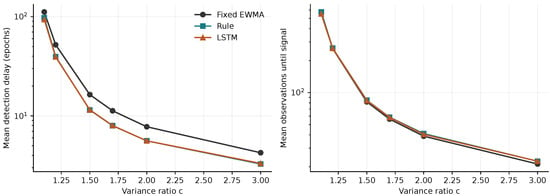
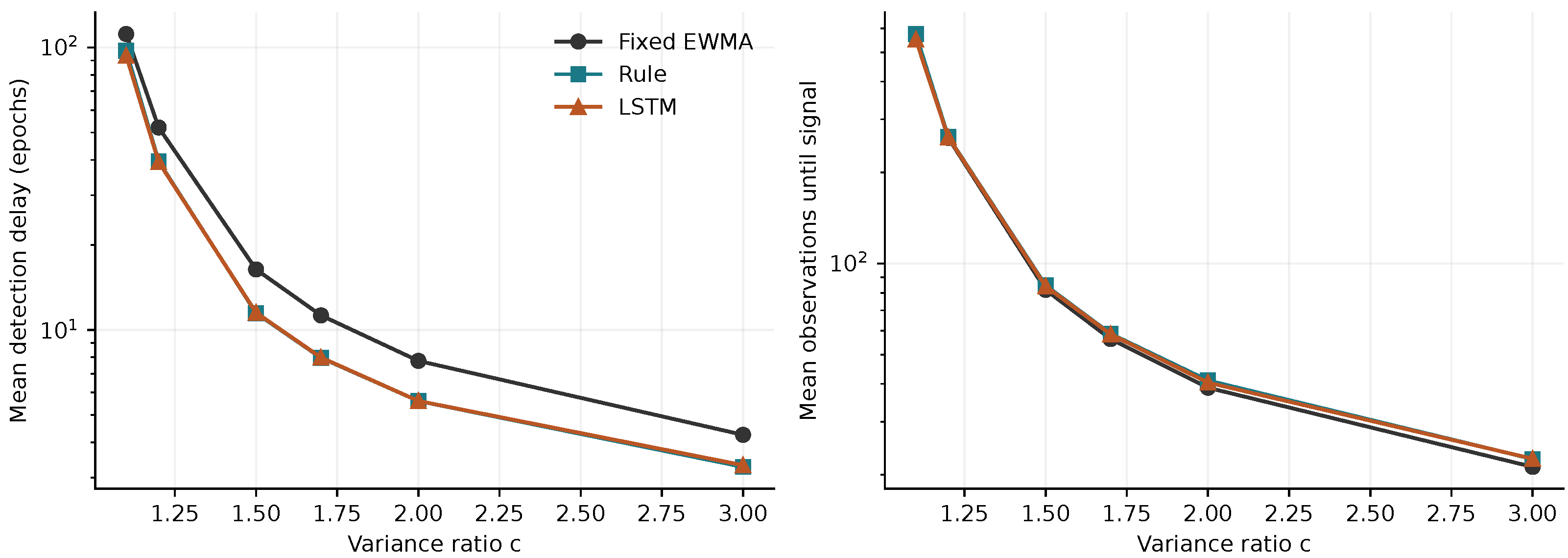
Table 3 and Figure 2 compare the fixed reference and the two budget-adjusted policies. At $c=1.5$, the LSTM delay is 11.51 epochs, versus 16.37 for fixed sampling and 11.47 for the rule. Thus, adaptive acquisition substantially reduces epoch-based delay in this setting, while the two adaptive policies have similar estimated delays. The corresponding measurement costs are 84.12, 81.87, and 84.63 observations. Faster detection is not accompanied by lower total measurement use relative to fixed sampling at this shift.

Table 3. Changes from epoch one. D is the mean detection delay in epochs, and C is the mean number of observations until a signal. Adaptive policies are the budget-adjusted configurations.

c	Fixed D	Fixed C	Rule D	Rule C	LSTM D	LSTM C
1.1	111.67	558.36	97.49	574.78	93.58	551.38
1.2	52.09	260.45	39.51	262.37	39.31	261.59
1.5	16.37	81.87	11.47	84.63	11.51	84.12
1.7	11.26	56.29	7.96	58.59	7.98	58.37
2.0	7.77	38.85	5.60	41.04	5.60	40.39
3.0	4.25	21.25	3.27	22.56	3.32	22.61

Figure 2. Delay and observation cost for changes from epoch one. Vertical axes use logarithmic scales. The curves show different consequences of increasing acquisition effort; they do not represent elapsed physical time.

For the smallest tested change, $c=1.1$, the LSTM has a mean delay of 93.58 epochs, compared with 97.49 for the rule and 111.67 for fixed sampling. This secondary comparison suggests that relative behavior can vary across change magnitudes. It does not establish a general advantage, and $c=1.1$ was not part of the optimization objective.

5.3. Changes After an In-Control Period

Table 4 presents conditional performance for a change in epoch 51. At $c=1.5$, the LSTM delay is 11.72 epochs and the rule delay is 11.87, compared with 16.46 for fixed sampling. At $c=2$, the ordering reverses slightly: 5.81 epochs for the LSTM and 5.73 for the rule. These comparisons involve the state distribution among trajectories surviving without an early alarm rather than a deterministic warm start. The raw results retain the survivor count and pre-change alarms for each configuration.

Table 4. Conditional performance after a change in epoch 51. D and C exclude pre-change epochs and costs, respectively, and condition on no earlier signal.

c	Fixed D	Fixed C	Rule D	Rule C	LSTM D	LSTM C
1.2	52.39	261.95	38.84	258.07	38.74	257.66
1.5	16.46	82.31	11.87	86.46	11.72	84.43
2.0	7.76	38.79	5.73	41.36	5.81	41.19

5.4. Aggregate Performance and Incremental Value of Recurrence

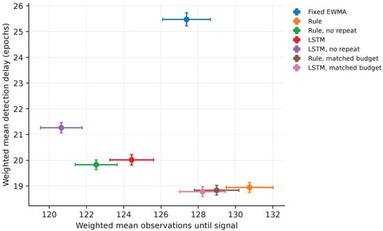
Table 5 summarizes the six-scenario means, and Figure 3 shows the corresponding delay–cost operating points. Across the six equally weighted design scenarios, the matched-budget rule has a mean delay of 18.84 epochs, and the LSTM has a mean delay of 18.78 epochs. The estimated relative reduction is 0.30%, with an approximate 95% Monte Carlo interval of $[-1.13\%,1.73\%]$. The interval does not contain a 10% reduction; this is not a prospectively powered test of that target. Nor does it establish equivalence: no formal equivalence test with a specified margin was conducted. The evidence supports only the narrower statement that a clear incremental detection advantage was not demonstrated in this experiment.

Table 5. Equally weighted means across $c\in \{1.2,1.5,2\}$ and change epochs 1 and 51. Costs are observations after the change.

Policy	$\overline{\mathit{D}}$	MCSE	$\overline{\mathit{C}}$	MCSE
Fixed EWMA	25.47	0.13	127.37	0.65
Rule	18.95	0.10	130.76	0.64
Rule, no repeat	19.83	0.10	122.52	0.58
LSTM	20.02	0.10	124.43	0.60
LSTM, no repeat	21.26	0.10	120.65	0.57
Rule, matched budget	18.84	0.10	128.99	0.61
LSTM, matched budget	18.78	0.10	128.23	0.63

Figure 3. Evaluated delay–cost operating points with approximate marginal 95% Monte Carlo intervals. This finite set is not an estimated global Pareto frontier. Policies also differ in in-control consumption and achieved false-alarm rate.

The ablations expose the role of the additional subgroup. For the selected rule, removing repetition increases weighted delay from 18.95 to 19.83 epochs while decreasing measurement cost from 130.76 to 122.52. For the selected LSTM, the corresponding changes are 20.02 to 21.26 epochs and 124.43 to 120.65 observations. Since limits are recalibrated and the no-repeat policies are not reoptimized, these results describe the evaluated configurations rather than an optimal value of resampling. They nevertheless show why a decision based only on delay would omit a material resource trade-off.

6. Experiment 2: Optimization, Learning-Based Policies, and Operational Sensitivity

6.1. Feedforward Comparator and Optimization-Budget Sensitivity

The additional comparator is a multilayer perceptron (MLP) with three hidden units,

$$H_k=\tanh (A{x}_k+b),A\in {\mathbb{R}}^{3\times 6},$$

(16)

using the same six inputs and the same two linear acquisition heads as the LSTM. Its hidden vector is initialized at zero before the first acquisition. It has 21 hidden-layer parameters, 6 head weights, and 3 thresholds: 30 optimized parameters. It retains the representation of the last acquired input until the next update but has no recurrent hidden-to-hidden connection. Both learning-based policies still receive the memory-bearing EWMA statistic. This comparison therefore examines extra recurrence beyond the common inputs, not all possible forms of temporal memory.

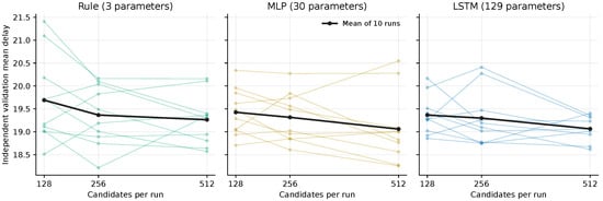
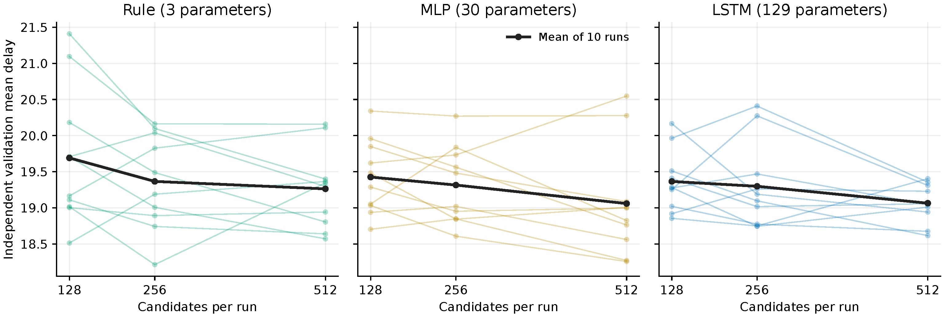
For each of the three families, three independent search runs, each initialized with a different seed, use 16 generations of 8 candidates, giving 384 evaluations per family, four times the budget in Experiment 1. Initialization, pilot sample sizes, and the penalty in Equation (14) are retained. An incumbent is reevaluated with the current generation, so a score from an earlier simulation batch is not compared directly with a new score. Checkpoints after 32, 64, and 128 evaluations per seed are independently validated. Each checkpoint uses ten limit-calibration steps with 1200 trajectories per step, 3000 in-control validation trajectories, and 1000 trajectories per detection scenario. Selection minimizes validated delay among checkpoints whose upper 95% consumption bound is at most five. The MLP, rule, and LSTM are selected separately, before the Experiment 2 test data are generated. Three seeds provide limited precision for estimating optimization variability. Their checkpoint results are supplied in the supplement. Table 6 and Figure 4 summarize the ten independent runs per family in Experiment 3, with checkpoints at 128, 256, and 512 candidates per run. Each checkpoint is calibrated with 2000 trajectories at each of 11 bisection steps, then assessed with 4000 in-control trajectories and 2000 trajectories per change scenario. Section 7 specifies the selection and test protocol. Experiments 2 and 3 use distinct selected configurations and independent final-test samples.

Table 6. Independent validation of ten search runs per family (Experiment 3). Candidates are counted per run; SD and range describe between-run variation in the validation objective. Feasible counts indicate the number of checkpoints whose upper 95% consumption bound does not exceed five. Rows describe fixed checkpoints, before checkpoint selection.

Family	Candidates	Mean D	SD	Range	Feasible
Rule	128	19.691	0.948	[18.513, 21.409]	10/10
Rule	256	19.366	0.663	[18.214, 20.163]	10/10
Rule	512	19.263	0.551	[18.571, 20.159]	10/10
LSTM	128	19.365	0.426	[18.854, 20.166]	9/10
LSTM	256	19.298	0.599	[18.744, 20.409]	10/10
LSTM	512	19.064	0.271	[18.615, 19.403]	10/10
MLP	128	19.426	0.518	[18.703, 20.340]	10/10
MLP	256	19.315	0.538	[18.608, 20.270]	10/10
MLP	512	19.059	0.772	[18.256, 20.548]	10/10

Figure 4. Optimization sensitivity with ten independent runs per family (Experiment 3). Thin colored lines show individual runs; the thick black line is their mean. Increasing the budget from 128 to 512 candidates does not by itself establish convergence. The resource condition is a common ceiling, not exact consumption matching.

Direct parameter search evaluates the complete acquisition policy through simulated trajectories. It does not estimate a value function, train a critic, or use temporal-difference updates. This choice permits a common optimizer across threshold and learning-based policies, but it does not imply that evolutionary search is preferable to reinforcement learning. Increasing search size is a sensitivity experiment, not proof of convergence. Differences between experiments also involve independent seeds and different incumbent handling; they cannot be attributed solely to the candidate count. Candidate counts alone also do not equalize parameter dimension, computation time, or attainable optimization accuracy.

6.2. Calibration and Independent Testing

The three policies selected through optimization, together with the fixed-size and matched-budget configurations from Experiment 1, undergo independent limit calibration: 13 bisection steps with 30,000 in-control trajectories per step. The acquisition weights of the Experiment 1 configurations are retained; only their alarm limits are recalibrated. Limits, policy parameters, and a hash manifest are frozen before testing. For each of six configurations, Experiment 2 uses 20,000 trajectories for each $c\in \{1,1.2,1.5,2\}$ at $\tau =1$ and 10,000 for each $c\in \{1.2,1.5,2\}$ at $\tau =51$: 660,000 test trajectories. No trajectory is censored. These data are independent of the 714,000 test trajectories in Experiment 1. Results are reported separately because the calibrated limits differ between experiments. Table 7 reports the in-control results for Experiment 2.

Table 7. Experiment 2 in-control evaluation, with target $AR{L}_0=370$ and 20,000 in-control trajectories per configuration ($c=1$, $\tau =1$). $|{\mathrm{\Delta }}_0|$ is absolute deviation from the target; the percentage column is signed relative deviation.

Policy	${\widehat{\mathit{ARL}}}_0$	MCSE	95% CI	$|{\mathbf{\Delta }}_0|$	${\mathbf{\Delta }}_0$ (%)	${\widehat{\mathit{ASN}}}_0$
Fixed EWMA	375.95	2.64	[370.77, 381.13]	5.95	+1.61	5.000
Rule, recalibrated	369.97	2.59	[364.90, 375.05]	0.03	−0.01	4.918
LSTM, recalibrated	370.11	2.61	[365.00, 375.23]	0.11	+0.03	4.917
Rule, extended search	368.61	2.54	[363.63, 373.60]	1.39	−0.38	4.838
LSTM, extended search	369.00	2.57	[363.96, 374.03]	1.00	−0.27	4.961
MLP, extended search	375.20	2.65	[370.01, 380.38]	5.20	+1.40	4.815

The simulator also records the number of additional subgroups acquired after the change, $R_{+}$. For all seven Experiment 1 configurations, verification trajectories confirm that recording this extra quantity leaves the other five simulated outputs unchanged. A zero-output MLP reproduces the rule under identical inputs and random seeds. This check verifies a limiting case; it does not imply that trained learning-based policies must agree.

The recalibrated matched-budget pair has nearly identical achieved $AR{L}_0$ values, 369.97 and 370.11, and consumption 4.9177 and 4.9167. Other configurations retain finite calibration error; the largest relative deviation from 370 is approximately 1.61%. The optimization-selected configurations satisfy the observed consumption budget but are not consumption-matched to one another. Consequently, the controlled recurrence comparison remains the recalibrated Experiment 1 pair, whereas the MLP comparison assesses attainable operating points under a common upper budget.

6.3. Detection and Bootstrap Uncertainty

Table 8 summarizes the six-scenario performance estimates, and Table 9 reports the conditional bootstrap contrasts.

Table 8. Experiment 2 test performance, equally weighted over the six detection scenarios. D is measured in epochs and C in individual observations. $R_{+}$ counts additional subgroups only after the change. $T_1=D+R_{+}$ is an additive duration proxy defined below.

Policy	$\overline{\mathit{D}}$	MCSE	$\overline{\mathit{C}}$	${\overline{\mathit{R}}}_{+}$	${\overline{\mathit{T}}}_1$
Fixed EWMA	25.383	0.101	126.92	0.000	25.383
Rule, recalibrated	18.860	0.076	128.81	3.782	22.642
LSTM, recalibrated	18.864	0.077	128.64	3.978	22.843
Rule, extended search	19.918	0.075	123.66	0.000	19.918
LSTM, extended search	19.064	0.076	126.97	2.075	21.138
MLP, extended search	18.874	0.076	127.28	4.322	23.196

Table 9. Bootstrap contrasts from Experiment 2 test trajectories. The 95% CIs are conditional percentile bootstrap confidence intervals; they are exploratory and not adjusted for multiple comparisons.

Contrast	$\mathbf{\Delta }\mathit{D}$	95% CI	R (%)	95% CI (%)
Recalibrated LSTM vs. rule	0.005	[−0.205, 0.216]	−0.03	[−1.16, 1.08]
Extended LSTM vs. MLP	0.190	[−0.017, 0.403]	−1.01	[−2.14, 0.09]

The recalibrated rule and LSTM have weighted delays of 18.860 and 18.864 epochs. At $c=1.5$ and $\tau =1$, their delays are 11.426 and 11.400 epochs, compared with 16.484 for fixed sampling. These scenario-specific reductions should be interpreted alongside the full weighted comparison and acquisition costs.

The 95% confidence intervals (CIs) for the delay contrasts are percentile intervals from 10,000 stratified nonparametric bootstrap replicates. Within each policy–scenario cell, surviving trajectories are independently resampled, and the six scenario means retain equal weights. Each CI is defined by the 2.5th and 97.5th percentiles of the bootstrap contrast. These CIs condition on the selected acquisition parameters, calibrated limits, and survival to the change epoch; they exclude optimization and calibration uncertainty. The same cell-level bootstrap replicates are used for the scenario-weight analysis in Section 6.6. For $\mathrm{\Delta }D={\overline{D}}_{\mathrm{LSTM}}-{\overline{D}}_{\mathrm{comparator}}$, a positive value favors the comparator. For the relative reduction $R=100(1-{\overline{D}}_{\mathrm{LSTM}}/{\overline{D}}_{\mathrm{comparator}})$, a positive value favors the LSTM.

The interval for the recalibrated difference is approximately $[-0.205,0.216]$ epochs; it supports neither a detectable LSTM gain nor formal equivalence. The extended-search LSTM has a weighted delay of 19.064 epochs, compared with 18.874 epochs for the MLP. The confidence interval for the LSTM-minus-MLP difference in weighted delay also includes zero. Thus, a competitive nonrecurrent mapping exists in this experiment, while the evidence remains insufficient to determine the performance attainable by other recurrent policies. The extended rule has a selected repeat threshold above one, so it never requests an additional subgroup before an alarm; its lower measurement cost accompanies a longer delay.

6.4. Measurement and Delay Costs

For measurement price $C_m>0$ and delay price $C_d\ge 0$, define the conditional operational loss

$$L=C_{m}C+C_{d}D,L/C_m=C+\rho D,\rho =C_d/C_m.$$

(17)

Prices are scenario assumptions in measurement-cost units, not estimates from an industrial installation. Table 10 evaluates the same frozen policies without reoptimization. The scripts retain the covariance between trajectory delay and observation count when calculating standard errors of this linear loss. The objective covers detection after a change; it excludes false-alarm intervention expenses, repair costs, training costs, and a long-run economic renewal model.

Table 10. Weighted normalized detection cost $\overline{C}+\rho \overline{D}$ under hypothetical delay prices. These are evaluated operating points, not economically optimized designs.

Policy	$\mathit{\rho }=0$	$\mathit{\rho }=1$	$\mathit{\rho }=5$	$\mathit{\rho }=20$
Fixed EWMA	126.92	152.30	253.83	634.58
Rule, recalibrated	128.81	147.67	223.11	506.01
LSTM, recalibrated	128.64	147.50	222.96	505.93
Rule, extended search	123.66	143.58	223.25	522.02
LSTM, extended search	126.97	146.03	222.29	508.24
MLP, extended search	127.28	146.16	221.65	504.76

The extended rule has lower observation use but longer delay than the recalibrated pair. Its apparent attractiveness therefore depends on the price attached to waiting. Very small differences between the recalibrated rule and LSTM should not be interpreted as economically meaningful without uncertainty analysis and application-specific prices.

6.5. Acquisition Duration Sensitivity

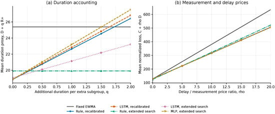
Suppose a base epoch has unit duration and an additional subgroup adds q units. A post-change duration proxy is

$$T_q=(T-\tau +1)+q{R}_{+},\mathbb{E}[T_q\mid T\ge \tau ]=D+q\mathbb{E}[R_{+}\mid T\ge \tau ].$$

(18)

Only additional subgroups acquired after the change enter this expression. Using the total number of repetitions, including those before the change, would overstate delayed-change acquisition overhead. For $q=1$, the extended rule has weighted duration 19.918 units, compared with 22.642 for the recalibrated rule and 22.843 for the recalibrated LSTM. The latter two still improve on the fixed policy’s 25.383 units, but their epoch advantage is reduced.

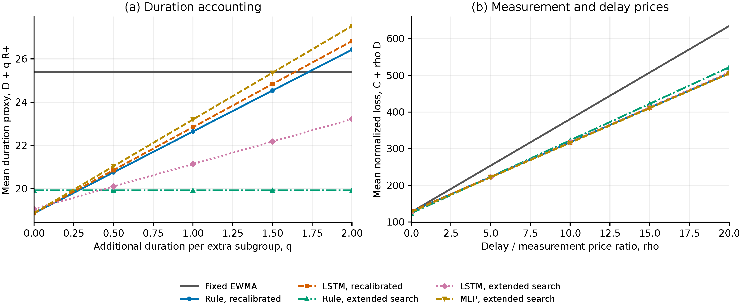
Figure 5 shows two different changes in operational accounting. In panel (a), $q=0$ recovers detection delay in epochs. The fixed and extended-rule lines are horizontal because neither policy acquires an additional subgroup. The recalibrated rule and LSTM start near 18.86 epochs but rise at slopes 3.782 and 3.978. Their duration curves cross the extended rule at approximately $q=0.280$ and $q=0.265$, respectively; these are illustrative break-even values from the estimated means. In panel (b), each curve starts at its mean measurement cost when $\rho =0$. Increasing $\rho$ places greater weight on delay, so the fixed policy’s larger delay produces a steeper line. The cost curves for the recalibrated rule and LSTM intersect the extended-rule curve at approximately $\rho =4.867$ and $\rho =4.721$, respectively. Near-overlap of the recalibrated curves reflects their small estimated differences and should not be read as a demonstrated economic advantage. Both panels transform existing trajectory summaries; they do not add new simulation observations or reoptimize policies.

Figure 5. Operational transformations of the six frozen Experiment 2 policies. (a) Mean duration $\overline{D}+q{\overline{R}}_{+}$: the intercept is epoch delay and the slope is the mean number of extra subgroups after the change. (b) Normalized loss $\overline{C}+\rho \overline{D}$: the intercept is measurement use and the slope is epoch delay. Panel (a) uses Table 8; panel (b) extends Table 10 continuously over $\rho$. Lower values are preferable for the stated assumption. Curves are point estimates, not uncertainty bands.

This calculation is not a simulation of a physical-time process. It assumes constant base-epoch duration regardless of the initial subgroup size, retains the change epoch used in the experiment, and adds serial resampling time after the fact. A model in physical time would also need to account for sample-size-dependent acquisition duration, scheduling, potentially overlapping measurements, and a change time defined on that physical clock.

6.6. Scenario and Weighting Sensitivity

Table 11 disaggregates the frozen-policy results, and the supplement supplies all six policies’ scenario means, costs, survivor counts, and standard errors. No policy is reselected using these tests. For nonnegative weights summing to one, the contrast is $\mathrm{\Delta }{D}_w={\sum }_s{w}_s(D_{\mathrm{LSTM},s}-D_{\mathrm{rule},s})$. Thus, over the complete weight simplex, its estimated value lies between the smallest and largest scenario contrasts, here $-0.195$ and $0.293$ epochs. These bounds describe the retained point estimates; they are not confidence bounds.

Table 11. Experiment 2 scenario-specific delays in epochs. R identifies the recalibrated policies; MLP is the extended-search policy. $\mathrm{\Delta }D$ is recalibrated LSTM minus recalibrated rule, so negative values favor the LSTM.

c	$\mathit{\tau }$	Fixed	Rule (R)	LSTM (R)	MLP	$\mathbf{\Delta }\mathit{D}$
1.2	1	52.419	39.387	39.192	39.872	−0.195
1.2	51	51.666	39.236	39.529	38.915	+0.293
1.5	1	16.484	11.426	11.400	11.512	−0.026
1.5	51	16.205	11.722	11.592	11.595	−0.129
2	1	7.782	5.598	5.644	5.594	+0.046
2	51	7.744	5.789	5.830	5.755	+0.040

The alternative shift weights are $(0.6,0.3,0.1)$ for small-shift emphasis and $(0.1,0.3,0.6)$ for large-shift emphasis, split equally between the two change epochs. Two additional summaries weight only changes at epoch 1 or epoch 51. The contrast changes sign between these time-specific summaries, and all five 95% CIs in Table 12 include zero. For each weight vector, the six scenario means are combined within each of the same 10,000 bootstrap replicates used in Table 9, and the 2.5th and 97.5th percentiles give the CI. Equal weighting therefore yields exactly the same estimate and CI in both tables. These conditional CIs reflect final-test Monte Carlo uncertainty and remain exploratory. The equal-weight mean is therefore one operational criterion, not a universal ranking. A worst-scenario delay ratio to the fixed policy is also supplied for each policy, allowing comparison without averaging raw delay over scenarios.

Table 12. Sensitivity of the recalibrated LSTM–rule contrast to scenario weights. The 95% CIs use the same stratified percentile bootstrap as Table 9, include final-test Monte Carlo error only, and are not adjusted for multiple comparisons.

Weighting	$\mathbf{\Delta }\mathit{D}$	95% CI
Equal	0.005	[−0.205, 0.216]
Small-shift emphasis	0.010	[−0.362, 0.383]
Large-shift emphasis	0.007	[−0.077, 0.090]
Change at epoch 1	−0.059	[−0.289, 0.175]
Change at epoch 51	0.068	[−0.291, 0.418]

7. Experiment 3: Repeated Search, Selection, Calibration, and Testing

7.1. Candidate and Computation Budgets

Ten independent search chains are run for each family, giving 30 optimizations. Ten repetitions characterize seed-to-seed variability within each family but do not constitute a power calculation or a convergence certificate. The architecture, parameter bounds, pilot sample counts, objective, and penalty are held fixed. Each generation contains eight candidates, including a reevaluated incumbent after the first generation. Two budget-based selection rules are applied to each search chain. The candidate-budget rule validates checkpoints after 128, 256, and 512 evaluations. The computation-budget rule uses checkpoints completed within 30 process-CPU seconds and the last complete generation before that limit. Search may continue to serve the other rule, but results obtained beyond the time budget cannot enter the time-budget selection. Each rule selects the feasible checkpoint with the lowest independent validation delay, subject to an upper 95% $AS{N}_0$ bound of five.

The 30 s limit covers proposal generation and pilot simulation, including pilot calibration. It excludes startup, validation, final calibration, and testing; separate stage timings are released. Process-CPU time excludes time spent waiting for processor scheduling. The selected stopping counts depend on hardware and numerical libraries. Recorded stopping generations permit replay with identical candidate counts, whereas enforcing the literal time limit on different hardware can change the evaluated candidate count. Across the ten runs, the cumulative number of candidates evaluated by the last eligible generation ranges from 592 to 632 for the rule, 344 to 376 for the MLP, and 168 to 200 for the LSTM. Matching this measured search budget addresses one aspect of computational fairness, while leaving differences in optimizer suitability and attainable optima unresolved.

Each selected checkpoint receives fresh limit calibration with 12,000 trajectories at each of 13 bisection steps. Testing then uses 20,000 in-control trajectories and 6000 trajectories in each of the six detection scenarios. The two budget rules have independent final-calibration and test streams, although they can select the same acquisition parameters. Frozen parameters, stage-specific seeds, calibration traces, and raw results are retained. All 60 selected policy–calibration combinations are tested, giving 3,360,000 test trajectories. Experiments 2 and 3 use the same C++ simulator. If a development or calibration cell contains a trajectory censored at 15,000 epochs, the entire cell is regenerated from the same seed with a 150,000-epoch cap and must finish without censoring. Such events are logged. No final-test trajectory is censored.

7.2. Variability Across Complete Repetitions

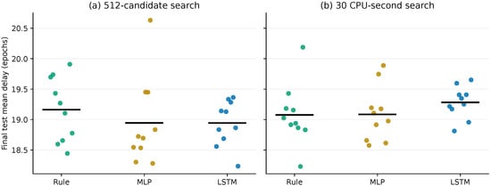
Table 13 and Figure 6 summarize the independent final tests. No chain is removed because it performs poorly. Table 14 pairs family runs by repetition index and reports t intervals with nine degrees of freedom for the mean of ten independently generated differences. Pairing uses the index only: simulation streams are independent across families. These intervals include variability from optimization, checkpoint selection, calibration, and finite final testing. These intervals quantify uncertainty in the mean difference between the specified search procedures. They do not quantify uncertainty in the conditional contrast between the two matched-budget policies in Experiment 2, nor do they provide a prediction interval for an individual future run.

Table 13. Experiment 3 final-test performance over ten independent chains per family and budget rule. SD is the between-chain standard deviation of weighted delay. Ranges show achieved in-control performance. Both budget rules validate checkpoints before testing; the candidate route has a maximum of 512 candidates.

Budget	Family	$\overline{\mathit{D}}$ (SD)	${\mathit{ARL}}_0$ Range	${\mathit{ASN}}_0$ Range
512 candidates	Rule	19.162 (0.528)	[357.6, 373.8]	[4.660, 4.947]
512 candidates	MLP	18.945 (0.720)	[365.2, 379.5]	[4.697, 4.956]
512 candidates	LSTM	18.943 (0.374)	[361.8, 372.6]	[4.675, 4.976]
30 CPU s	Rule	19.076 (0.500)	[363.0, 379.6]	[4.705, 4.942]
30 CPU s	MLP	19.085 (0.449)	[359.0, 377.6]	[4.763, 4.920]
30 CPU s	LSTM	19.282 (0.262)	[364.5, 379.0]	[4.718, 4.891]

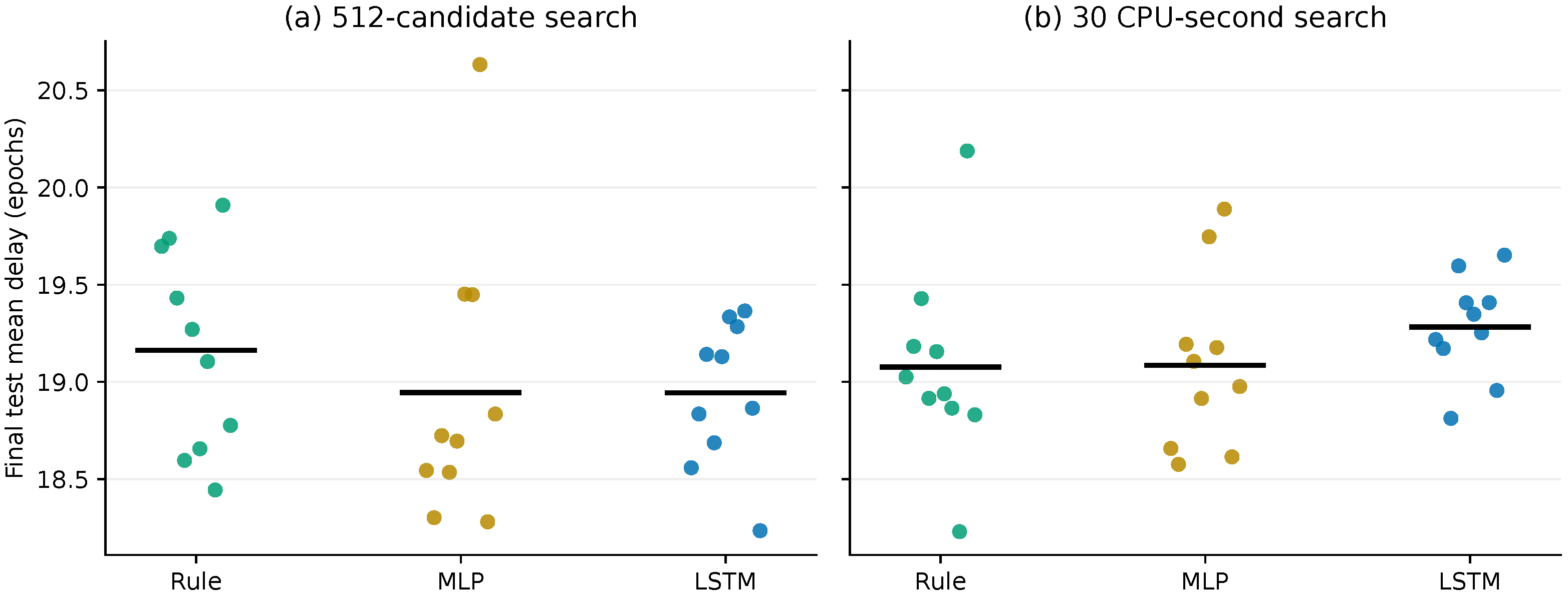
Figure 6. Final-test delay from each complete optimization, selection, and calibration repetition. Each point is one run; horizontal bars mark family means. Panel (a) uses the candidate-budget rule and panel (b) uses the process-CPU budget. The panels share search chains but have independent final-calibration and test streams.

Table 14. Experiment 3 mean delay contrasts with variability across complete repetitions. Negative values favor the LSTM. Intervals are exploratory and unadjusted for multiple comparisons. They apply to the specified finite search and selection procedures.

Budget	Contrast	$\mathbf{\Delta }\mathit{D}$	Across-Run 95% Interval
512 candidates	LSTM–Rule	−0.219	[−0.723, 0.285]
512 candidates	LSTM–MLP	−0.001	[−0.416, 0.413]
30 CPU s	LSTM–Rule	+0.206	[−0.295, 0.708]
30 CPU s	LSTM–MLP	+0.197	[−0.130, 0.524]

Under the candidate-budget rule, the mean LSTM–rule difference is −0.219 epochs (95% interval [−0.723, 0.285]); under the CPU-budget rule it is +0.206 epochs (95% interval [−0.295, 0.708]). The corresponding LSTM–MLP differences are −0.001 epochs (95% interval [−0.416, 0.413]) and +0.197 epochs (95% interval [−0.130, 0.524]). These contrasts are reported alongside achieved $AR{L}_0$ and $AS{N}_0$ because the Experiment 3 runs share a consumption ceiling but are not matched exactly in false-alarm rate or observation use. All observed final-test consumption estimates are below five. The observed differences can therefore reflect both the search procedure and the selected operating point; they cannot be assigned solely to recurrent memory. Increasing candidate counts gives a broader sensitivity analysis, while the remaining variation in Figure 4 prevents a claim that all families reached their attainable optima.

8. Discussion

The framework separates acquisition decisions from alarm generation and makes their resource consequences explicit. In Experiments 1 and 2, the evaluated adaptive configurations have shorter epoch-based delays than the fixed-size reference over the specified scenarios. Their observation and duration costs differ, however, and the policy preferred under one operational criterion can be unattractive under another. This distinction is directly relevant to automated inspection, where measurement opportunities and the time available before intervention are both limited.

The recalibrated matched-budget comparison does not demonstrate an incremental recurrence benefit. The competitive MLP provides additional evidence that the six common inputs can support an effective feedforward policy in this model. These observations do not establish that recurrent memory is unnecessary: both learning-based policies are compact, the optimization budget is finite, and the existing EWMA input already carries historical information. Nonmonotonic budget curves show that optimization uncertainty remains a plausible contributor to the results. Experiment 3 assesses this variability through ten complete repetitions per family and a separate computation-budget rule. Its intervals describe the output of the tested search and selection procedures and must be distinguished from the conditional intervals in Experiment 2. All three experiments evaluate finite procedures and selected operating points rather than the theoretical capacity of each model class. In particular, the Experiment 2 MLP–LSTM confidence interval includes zero and does not establish MLP superiority.

8.1. Position Relative to Published Methods

Haq’s adaptive dispersion EWMA and the sample-size strategy of Abbasi and Noor-ul-Amin [3,4] are relevant external comparators. They adapt different components from the common-detector acquisition experiment conducted here. Their published methods have not been numerically reproduced in this study. Accordingly, every numerical performance conclusion is restricted to the fixed, rule-based, MLP, and LSTM configurations evaluated here. No practical advance in detection efficiency over established adaptive dispersion charts is claimed. The fixed-size reference is an internal baseline and is not a proxy for the state of the art. An external benchmark remains necessary to establish such a practical advance. It would require a verified implementation and compatible initialization, variance-change definitions, false-alarm calibration, and observation accounting. Allowing repeated sampling until a decision, for example, changes the per-epoch action space relative to the one-extra-subgroup limit used here. The coefficient of variation formulation of Ahmadini et al. [5] additionally requires a compatible mean model. Published ARLs cannot be transferred directly between these settings.

Predictive LSTM monitoring for data with time-varying variability [8] addresses another role for learning: prediction and uncertainty modeling. The present network instead controls acquisition for a fixed detector. Similarly, economic-statistical designs [16] motivate explicit prices, but the sensitivity analysis here does not estimate a full economic objective. These distinctions position this study as a contribution to reproducible policy comparison and operational accounting.

Table 15 separates acquisition control from learning the alarm statistic or recognizing patterns. External methods are not assumed to share the observation budget, change definition, or time accounting used here. Their numerical ranking would require compatible implementations and calibration.

Table 15. Position of the study relative to selected literature. Entries identify the monitored quantity, the component being adapted or learned, and the evaluation emphasis described by the cited sources. This is a methodological comparison, not a numerical performance ranking.

Study	Monitored Quantity or Task	Adaptive or Learning Component	Evaluation Emphasis
Haq [3]	Process dispersion	Shift-dependent EWMA smoothing	Run-length behavior over dispersion shifts
Abbasi and Noor-ul-Amin [4]	Process dispersion	Sample-size strategy with quadratic-sigmoid EWMA	Detection sensitivity and run-length comparisons
Ahmadini et al. [5]	Coefficient of variation	Variable sample size in EWMA	Performance under a coefficient-of-variation formulation
Aslam et al. [6]	Process variance	Repetitive sampling with inner and outer limits	ARL and average sample number
Qiu et al. [8]	Predictive monitoring	LSTM prediction intervals	Monitoring with time-varying variability
Zan et al. [9]	Histogram and chart patterns	Bidirectional LSTM feature learning	Pattern-recognition accuracy
Chiu and Fu [10]	Mixture chart patterns	Hybrid CNN–LSTM	Online recognition in autocorrelated processes
Suárez Castro and Ladino Vega [11]	EWMA temperature values	LSTM approximation	Prediction error for individual measurements
Present study	Process variance	Rule-based or learning-based sample sizes; one optional repeat; common EWMA alarm	Independently calibrated ARL; epoch delay; observations; cost and duration sensitivity

8.2. Threats to Validity

Internal validity. Causal sample-size selection, fresh subgroups, and explicit counting are enforced by the simulator. Verification includes the normal-score transformation, bounded resampling, agreement between simulator outputs with and without the additional repetition record, and the fixed-size accounting identity. Finite calibration errors persist outside the closely matched pair. Published adaptive comparators remain unimplemented.

External validity. This study assumes independent normal observations, known reference variance, and permanent variance increases. Estimated parameters, autocorrelation, nonnormality, gradual faults, and industrial data require separate experiments. Estimated-parameter dispersion charts [17] illustrate one such extension. The present evidence does not establish deployment performance.

Construct validity. Epoch delay, individual measurements, and subgroup acquisition duration are distinct quantities. The cost and duration scenarios expose this distinction but use assumed prices and timing. The MLP retains EWMA information and the most recent input representation; it is nonrecurrent at the network level rather than devoid of historical information.

Statistical conclusion validity. Bootstrap intervals condition on frozen policies and calibration. The conditional intervals in Experiment 2 exclude uncertainty across complete optimization and calibration repetitions; the across-run intervals in Experiment 3 address that separate estimand. Neither the three-seed design in Experiment 2 nor the ten-run design in Experiment 3 establishes global optimality or convergence, especially for the 129-parameter LSTM. In Experiment 3, this limitation applies to both the candidate-budget rule, with up to 512 candidate evaluations per run, and the separate computation-budget rule. Experiment 3 quantifies variability across complete search, selection, and calibration repetitions for the same finite algorithm; ten repetitions still provide limited precision for characterizing the sampling distribution of the resulting performance estimates. Selection among validation checkpoints can favor noisy estimates; fresh testing mitigates evaluation bias but does not eliminate optimizer variability. Scenario comparisons remain exploratory, and a nonsignificant difference is not an equivalence result.

9. Conclusions

A causal acquisition framework couples predictable subgroup sizes and at most one additional subgroup per epoch to a common EWMA variance detector. The matched-budget comparison in Experiment 2 gives weighted delays of 18.860 and 18.864 epochs for the recalibrated rule and LSTM; the conditional confidence interval for the difference in their weighted delays includes zero. This result concerns those selected policies. It does not establish equivalence of the policy families or show that recurrence can never be useful.

Ten independent optimization chains per family, broader candidate budgets, independent calibration, and a process-CPU budget provide a more direct assessment of search variability. The resulting contrasts characterize the specified finite procedures and their operating points. Scenario weights, observation prices, and the duration of an extra subgroup affect the interpretation of performance, so neither an equally weighted delay nor the results from a single selected search run establish a universal ranking. The study supports reproducible comparison within the common-detector framework. Numerical comparison with established adaptive dispersion charts and validation under application-specific process and timing models remain necessary to assess a practical advance beyond this framework.

References

- Costa, A.F.B. Charts with Variable Sample Size. J. Qual. Technol. 1994, 26, 155–163. [Google Scholar] [CrossRef] [Scilit]
- Castagliola, P. A New S2-EWMA Control Chart for Monitoring the Process Variance. Qual. Reliab. Eng. Int. 2005, 21, 781–794. [Google Scholar] [CrossRef] [Scilit]
- Haq, A. A new adaptive EWMA control chart for monitoring the process dispersion. Qual. Reliab. Eng. Int. 2018, 34, 846–857. [Google Scholar] [CrossRef] [Scilit]
- Abbasi, A.R.; Noor-ul-Amin, M. Adaptive sample size strategies for process dispersion using EWMA control chart. Qual. Reliab. Eng. Int. 2025, 41, 510–531. [Google Scholar] [CrossRef] [Scilit]
- Ahmadini, A.A.H.; Khan, I.; Alshammari, A.O.; AlQadi, H.; Sumelka, W. Adaptive VSS-EWMA control chart for monitoring the process dispersion. Sci. Rep. 2025, 15, 21795. [Google Scholar] [CrossRef] [Scilit]
- Aslam, M.; Khan, N.; Jun, C.-H. A new S2 control chart using repetitive sampling. J. Appl. Stat. 2015, 42, 2485–2496. [Google Scholar] [CrossRef] [Scilit]
- Tran, P.H.; Ahmadi Nadi, A.; Nguyen, T.H.; Tran, K.D.; Tran, K.P. Application of Machine Learning in Statistical Process Control Charts: A Survey and Perspective. In Control Charts and Machine Learning for Anomaly Detection in Manufacturing; Tran, K.P., Ed.; Springer: Cham, Switzerland, 2022; pp. 7–42. [Google Scholar] [CrossRef] [Scilit]
- Qiu, J.; Lin, Y.; Zwetsloot, I.M. An LSTM-based predictive monitoring method for data with time-varying variability. Int. J. Prod. Res. 2025, 63, 2622–2637. [Google Scholar] [CrossRef] [Scilit]
- Zan, T.; Liu, Z.; Su, Z.; Wang, M.; Gao, X.; Chen, D. Statistical Process Control with Intelligence Based on the Deep Learning Model. Appl. Sci. 2020, 10, 308. [Google Scholar] [CrossRef] [Scilit]
- Chiu, J.-E.; Fu, S.-Z. On-line recognition of mixture control chart patterns using hybrid CNN and LSTM for auto-correlated processes. Comput. Ind. Eng. 2024, 198, 110674. [Google Scholar] [CrossRef] [Scilit]
- Suárez Castro, R.M.; Ladino Vega, I.D. Redes neuronales aplicadas al control estadístico de procesos con cartas de control EWMA. Tecnura 2023, 27, 72–88. [Google Scholar] [CrossRef] [Scilit]
- Banerjee, T.; Veeravalli, V.V. Data-Efficient Quickest Change Detection with On-Off Observation Control. arXiv 2011, arXiv:1105.1361v3. [Google Scholar]
- Nitinawarat, S.; Veeravalli, V.V. Controlled Sensing for Sequential Multihypothesis Testing with Controlled Markovian Observations and Non-Uniform Control Cost. arXiv 2014, arXiv:1310.1844v2. [Google Scholar]
- Hochreiter, S.; Schmidhuber, J. Long Short-Term Memory. Neural Comput. 1997, 9, 1735–1780. [Google Scholar] [CrossRef] [Scilit]
- de Boer, P.-T.; Kroese, D.P.; Mannor, S.; Rubinstein, R.Y. A Tutorial on the Cross-Entropy Method. Ann. Oper. Res. 2005, 134, 19–67. [Google Scholar] [CrossRef] [Scilit]
- Castagliola, P.; Celano, G.; Fichera, S. Economic-statistical design of an S EWMA control chart for monitoring process variability. J. Qual. Maint. Eng. 2007, 13, 304–320. [Google Scholar] [CrossRef] [Scilit]
- Ong, K.; Teh, S.; Soh, K.; Chong, Z.L.; Khoo, M.B. Optimal Design of S2-EWMA Control Chart with Estimated Parameters Based on Median Run Length and Expected Median Run Length. Qual. Reliab. Eng. Int. 2025, 41, 1495–1532. [Google Scholar] [CrossRef] [Scilit]
Disclaimer/Publisher’s Note: The statements, opinions and data contained in all publications are solely those of the individual author(s) and contributor(s) and not of MDPI and/or the editor(s). MDPI and/or the editor(s) disclaim responsibility for any injury to people or property resulting from any ideas, methods, instructions or products referred to in the content. |
© 2026 by the authors. Licensee MDPI, Basel, Switzerland. This article is an open access article distributed under the terms and conditions of the Creative Commons Attribution (CC BY) license.