


Abstract
Ramp metering regulates the rate at which vehicles enter a freeway and can reduce congestion when several entrance ramps compete for limited mainline capacity. Coordinating multiple ramps requires a traffic model that captures how present metering decisions influence later traffic conditions across the corridor. This study develops a coordinated ramp-metering framework based on METANET (Modèle d’Écoulement de Trafic sur Autoroute NETworks), a second-order macroscopic model in which traffic density and average speed evolve dynamically. Minimum and bounding operations are replaced with smooth differentiable approximations while preserving vehicle conservation, nonnegative flows and queues, and physically admissible traffic states. A discrete adjoint formulation computes sensitivities to the full sequence of metering decisions, and the control problem is solved using bound-constrained optimization with penalty continuation. The framework is evaluated on a 12-mile westbound section of Interstate 210 in Pasadena, California, with six metered ramps. The optimized policy reduces total delay by 5.86% relative to uncontrolled operation, compared with 0.27% for a jointly tuned ALINEA benchmark, while maintaining identical vehicle-miles traveled and remaining within the prescribed ramp-storage tolerance. The improvement is driven mainly by temporal redistribution of ramp arrivals and is limited by ramp storage and metering capability.
1. Introduction
A freeway carries a limited amount of traffic during a given period. This limit is commonly referred to as traffic capacity and is typically expressed in vehicles per hour. The traffic attempting to enter the freeway during the same period is referred to traffic demand; congestion can develop when demand approaches or exceeds the available capacity. This situation is particularly important near an on-ramp, where vehicles entering from a local road must merge with vehicles already traveling on the freeway mainline—meaning the continuous roadway through which freeway traffic travels [1]. If the combined mainline and ramp traffic becomes too large, vehicles begin to interact more strongly, average speed decreases, and traffic density, measured as the number of vehicles occupying a unit length of roadway, increases [2]. A persistent, congested region can then form and extend upstream from the location where traffic is restricted [3]. The result is additional travel-time and waiting time for the vehicles using the corridor.
One method for managing this problem is to install a traffic signal on an entrance ramp, known as a ramp meter, which regulates the rate at which vehicles are allowed to enter the freeway [4]. Its control variable is therefore a metering rate of vehicles, expressed in vehicles per hour. Restricting ramp entry for a short period can prevent too many vehicles from reaching an already heavily loaded mainline at the same time. This control, however, creates a competing effect: vehicles that are not immediately released remain on the ramp and form a ramp queue. Each ramp has finite physical storage capacity for this queue of vehicles. If the queue becomes longer than the available storage, it may extend into the adjoining surface-street network. A useful ramp-metering strategy must consequently consider both sides of the problem: reducing congestion on the freeway while preventing excessive waiting and queue growth on the ramps [5].
When several entrance ramps are located along the same freeway corridor, controlling each ramp independently may not provide the most effective overall traffic condition. As illustrated in Figure 1, vehicles entering from an upstream ramp join the freeway mainline and continue toward downstream locations. Their release therefore affects the amount of traffic encountered farther along the corridor [6]. When the combined traffic demand approaches the available freeway capacity, congestion can develop near the merge and propagate upstream. At the same time, restricting ramp entry creates a queue behind the ramp meter, and this queue cannot exceed the limited physical storage available on the ramp. Coordinated ramp metering therefore considers the entrance ramps together so that ramp traffic can be distributed across the corridor without creating excessive mainline congestion or unacceptable ramp queues [5]. The difficulty is that the influence of each ramp’s traffic release on downstream traffic conditions and on the allowable releases from other ramps varies continuously across both space and time. A metering decision made at one ramp changes the traffic entering the main-line and can subsequently influence traffic conditions at downstream locations. Its effect may also continue after the original metering decision has changed. Determining suitable ramp releases therefore requires a traffic model that can represent how traffic moves through the corridor and how current control decisions influence later traffic conditions [5,7].
Figure 1.
Conceptual representation of freeway congestion, ramp metering, and finite ramp-storage constraints.
Coordinated ramp metering has evolved from local feedback control toward corridor- and network-level strategies that account for interactions among multiple entrance ramps and downstream bottlenecks. Recent studies have broadened this scope by considering mixed-autonomy traffic and explicit safety constraints in ramp-metering design [8,9], as well as integrated control frameworks that combine ramp metering with variable speed limits, traffic signals, perimeter control, and other freeway-management measures [10,11,12,13,14]. Parallel developments have introduced data-driven and learning-based coordination, including physics-informed reinforcement learning, causal-effect-based control, demonstration-guided deep reinforcement learning, reinforcement-learning-based freeway control, and attention-based coordinated ramp metering [15,16,17,18,19]. Ramp-control concepts have also been extended to automated and lane-free traffic environments through direct coordination of ramp-vehicle behavior [20]. Although these methods differ substantially in their control structures, they share the objective of coordinating ramp inflows according to conditions beyond an individual entrance ramp.
For model-based coordinated control, determining appropriate ramp releases requires a traffic representation capable of describing how current metering decisions influence later traffic conditions across both location and time. Messmer & Papageorgiou (1990) [21] developed a second-order macroscopic model for motorway networks named METANET (Modèle d’Écoulement de Trafic sur Autoroute NETworks). In a second-order model, both traffic density and average speed evolve dynamically, allowing the model to represent how traffic conditions develop and propagate along the freeway. METANET has subsequently been applied and evaluated for large-scale freeway networks and remains a widely used basis for model-based freeway control [22]. Second-order macroscopic models have also been used directly for coordinated ramp-metering control. Kotsialos (2021) [23], for example, formulated coordinated ramp metering using a multi-class second-order macroscopic model and solved the resulting optimization problem through Differential Evolution. More recently, Chuka et al. (2026) [24] applied METANET within a feedback-linearization and model-predictive-control framework for coordinated ramp metering. These studies demonstrate the continued applicability of second-order models to freeway control, although their solution procedures do not propagate gradients directly through the original nonlinear traffic dynamics.
Gradient-based methods provide another route for solving large-coordinated control problems because they use the sensitivity of traffic performance to make changes in the control decisions. Reilly et al. (2015) [25] derived a discrete adjoint for traffic networks governed by first-order scalar conservation laws and applied it to coordinated ramp metering, demonstrating that sensitivities with respect to many control decisions can be obtained efficiently. For second-order traffic models, Poole & Kotsialos (2016) [26] incorporated automatic differentiation into METANET and used the resulting derivatives for model calibration. These studies establish the usefulness of adjoint-based sensitivities for ramp-metering control and the feasibility of differentiating a METANET implementation, respectively, but they address different traffic-model structures and optimization purposes.
A further difficulty arises because several traffic movements in macroscopic models are governed by multiple physical limits. For example, the actual flow released from an entrance ramp cannot exceed the rate allowed by the ramp-meter, the number of vehicles available on the ramp, or the additional traffic that the downstream freeway can receive. The realized ramp flow is therefore determined by the most restrictive of these limits. Other quantities must similarly remain within physically meaningful ranges. These restrictions are commonly represented by minimum and clipping operations. The main mathematical difficulty is that such hard limiting operations can produce undefined or locally zero derivatives. In a conventional minimum operation, the controlling limit changes abruptly when two competing limits become equal; at that switching point, a unique derivative does not exist, while away from it the noncontrolling limits may contribute no local sensitivity to the result. This behavior can interrupt the propagation of control sensitivities through the simulated traffic trajectory and thereby reduce the reliability of the gradient used to update ramp-metering decisions.
A smooth approximation replaces this abrupt switch with a narrow continuous transition, allowing both the calculated traffic quantity and its derivative to vary continuously as traffic conditions change. Such smoothing techniques are widely used in numerical optimization to replace nonsmoothed relationships with differentiable approximations while retaining their limiting behavior [27,28]. In traffic-control applications, Gu et al. (2022) [29] applied this principle to ramp-metering optimization based on the first-order Cell Transmission Model by replacing hard minimum operators with smooth approximations. The approach has subsequently been extended to coordinated ramp-metering and variable-speed-limit control using smoothed first-order traffic dynamics and co-state-based gradients [30]. These developments are closely related to the present study but remain based primarily on first-order traffic models. A second-order formulation introduces an additional dynamic equation for vehicle speed and therefore requires differentiability to be maintained not only through vehicle-flow relations but also through the evolving speed dynamics and associated physical limits. Recent work has separately addressed the physical admissibility of second-order models. Zhao et al. (2025) [31], for example, developed Bounded-METANET to prevent unrealistic speed values without relying on an external speed-saturation operation. However, its ramp-flow formulation retains a hard minimum among competing physical limits, and the study focuses on traffic-model formulation and calibration rather than differentiable coordinated ramp-control optimization.
Despite these developments, an important methodological gap remains. Smoothing-based ramp-metering optimization has been developed primarily for first-order traffic models, particularly Cell Transmission Model formulations, including recent coordinated ramp-metering and variable-speed-limit control based on smoothed CTM dynamics and co-state gradients. In contrast, second-order METANET-based studies retain explicit speed dynamics but have generally relied on alternative solution approaches rather than differentiating the complete nonlinear traffic evolution. Recent Bounded-METANET improves the physical admissibility of second-order traffic states by inherently bounding speed, but its origin-flow formulation retains hard limiting operations and was developed primarily for traffic-model formulation rather than differentiable coordinated ramp-metering optimization. Thus, the unresolved problem is not second-order modeling, smoothing, or coordinated control individually, but their integration within a physically admissible and differentiable optimization framework over the relevant operating domain. Accordingly, the specific research objective of this study is to determine a coordinated ramp-metering policy that minimizes corridor-wide traffic delay while maintaining ramp-storage and physically admissible traffic-state limits, using a differentiable second-order METANET-family model with discrete-adjoint sensitivity analysis. The resulting policy is evaluated using total delay, peak ramp queue, and total vehicle travel. Total delay measures the reduction in congestion, peak ramp queue assesses operational feasibility under finite storage capacity, and total vehicle travel confirms that the improvement is achieved without reducing the amount of traffic served. Together, these measures determine whether the proposed differentiable second-order optimization framework produces both meaningful traffic-performance improvements and physically implementable coordinated metering decisions.
2. Model Development
Following the stated research objective, the study is carried out through six sequential steps:
- Develop the differentiable traffic model. The conventional hard minimum and clipping operations in the METANET-based formulation are replaced with smooth counterparts while preserving vehicle conservation, nonnegative flows and queues, and physically admissible density and speed trajectories.
- Construct and verify the control gradient. A discrete adjoint formulation is derived to obtain the sensitivity of the objective function to the complete sequence of ramp-metering decisions. The resulting gradient is checked against central finite differences, including the zero-demand and zero-queue boundary condition.
- Determine the coordinated ramp-metering solution. The verified model and gradient are used to optimize the ramp-metering rates subject to the prescribed operating and ramp-storage limits, and the resulting traffic performance is evaluated relative to uncontrolled operation using total delay, peak ramp queue, and vehicle-miles traveled.
- Evaluate the optimized control against the benchmark strategy. The resulting coordinated policy is compared with a jointly tuned ALINEA feedback controller under the same demand, control bounds, objective function, and feasibility requirements.
- Examine the treatment of control bounds. Direct bounded optimization and unconstrained reparameterization are compared using the attained objective value and projected-gradient residual to assess their numerical behavior within the same optimization problem.
- Assess the control mechanism and operational sensitivity. The optimized solution is examined by removing the merge-related speed effect and varying ramp-storage capacity and the metering-rate ceiling to determine the physical mechanism governing the control-benefit and the operational conditions that limit its effectiveness.
The notations are grouped into indices, state variables, decision variables, exogenous data, and parameters, and each symbol is given with its physical unit so that the model can be reproduced in the units used here.
- (a)
- Indices and sets
- Represents mainline segment, numbered in the direction of travel where .
- Indicates metered on-ramp; ramp merges into segment , .
- Uncontrolled off-ramp, located in segment , .
- Time index; the control is applied at .
- (b)
- Traffic flow parameters
- Exponent shaping the speed-density relation.
- Free-flow speed of vehicles (miles/h).
- Critical density, at which flow is greatest (veh/mile/lane).
- Traffic-jam density, at which traffic stops (veh/mile/lane).
- Time drivers take to adjust toward the equilibrium speed (h).
- Anticipation constant (mile2/h).
- Traffic-density constant used to prevent division by zero (veh/mile/lane).
- Merging coefficient governing the merge speed disturbance.
- Fraction of flow diverted at off-ramp .
- Mainline capacity (vehicle/h).
- Physical capacity of ramp (vehicle/h).
- Lower speed clamp used for numerical safety (mile/h).
- Length of one segment (miles).
- Number of Lanes per segment.
- Duration of one control interval (h).
- Number of control intervals in the planning horizon.
- Traffic flow leaving segment (vehicle/h).
- Receiving factor of segment , between zero and one.
- Flow of vehicles admitted from ramp (vehicle/h).
- Flow of vehicles at the mainline entry (vehicle/h).
- Equilibrium speed at density (mile/h).
- Demand of vehicles arriving at the mainline entry (vehicle/h).
- Demand of vehicles arriving at ramp (vehicle/h).
- Vehicle density imposed at the downstream boundary (veh/mile/lane).
- Mainline traffic flow used to initialize the corridor (vehicle/h).
- Smallest and largest permitted metering rates (vehicle/h).
- Storage capacity of ramp (vehicles).
- Storage capacity at the mainline entry (vehicles).
- (c)
- Smoothing, weighting and tolerance parameters
- Sharpness of the smooth minimum.
- Widths of the two smooth saturations.
- Penalty weights on queue and density violation.
- Weight on the control-smoothness term.
- Terminal clearance-time coefficient (h).
- Factor by which penalty weights are raised between continuation steps.
- (d)
- State variables
- Traffic density in segment at time (veh/mile/lane).
- Space-mean speed of vehicle in segment at time (mile/h).
- Number of vehicles queued on ramp at time (vehicles).
- Number of vehicles queued at the mainline entry at time (vehicles).
- (e)
- Decision variables
- Metering rate posted at ramp at time (vehicle/h).
- The variable optimized as normalized metering rate where .
- Unconstrained surrogate used by the logistics-reparameterization (), .
The notation introduced above provides the complete mathematical description of the corridor, traffic-flow dynamics, smoothing parameters, state variables, and control decisions used in the formulation. These quantities are used consistently throughout the model development to represent traffic evolution, operational limits, and ramp-metering control within a unified optimization framework.
2.1. Differentiable Approximation of Nonsmooth Operators
Several traffic flows are restricted simultaneously by more than one physical condition. These restrictions are referred to here as competing flow limits, meaning nonnegative upper bounds on the same traffic flow. For example, a ramp may be permitted to release 600 veh/h by its meter, have enough vehicles available to provide 750 veh/h, but the downstream freeway may currently be able to receive only 500 veh/h. The actual ramp flow cannot exceed any of these values and must therefore be governed by the smallest limit, 500 veh/h. A flow limit can also equal zero, such as when no vehicle is available on an empty ramp. For competing traffic flow-limits , the physically exact relation would be . The hard minimum is suitable for forward simulation, but its derivative changes abruptly when the identity of the smallest argument changes. To obtain a differentiable approximation while retaining the role of the smallest physical limit, the following negative-power smooth minimum is used:
Equation (1) follows from the fact that raising positive numbers to a large negative power emphasizes the smallest number. For example, if , then , and this difference becomes increasingly pronounced as increases. The summation is therefore dominated progressively by the smallest , after which the power returns the result to the original physical unit of the inputs. Consequently, . Thus, is a positive and dimensionless sharpness parameter. There is no finite mathematical upper bound on ; increasing it makes the approximation closer to the hard minimum, although excessively large values can create numerical difficulties. If any , the physical minimum is exactly zero, and Equation (1) is therefore defined to return zero directly. Its conservativeness can be proved directly. Let, and since every , . At least one term is exactly , while at most terms can have that value. Hence, . Taking both sides to the power reverses the inequalities and gives . Therefore, the smooth minimum never exceeds the true minimum. This is important physically because the calculated ramp flow cannot be allowed to exceed the amount permitted by any of its limiting conditions. Therefore, the relative approximation error is the fraction by which the smooth value falls below the true minimum, and from the preceding bound, its maximum possible value is . This bound quantifies only the approximation error introduced by replacing the hard minimum with the smooth-minimum operator; it is not a measure of the total modeling error of the underlying METANET traffic model, parameter specification, demand representation, or numerical experiment.
Equation (1) is mathematically simple but can be difficult to evaluate directly on a computer. If is small and is large, the quantity can become extremely large. If it exceeds the largest number that the computer can represent, numerical overflow occurs. Here, overflow refers only to computer arithmetic; it does not mean traffic or queue spillback. Starting from Equation (1), . If we define , then, and factoring from the summation provided, . Substituting this result into Equation (1) yields,
Since is the smallest , every . Therefore, every exponent in Equation (1) is non-positive and every exponential term is at most one. This prevents excessively large intermediate values and makes Equation (2) numerically more stable than direct evaluation of Equation (1).
Gradient-based optimization also requires the derivative of the realized flow with respect to each competing limit. Let, and . Since, , the derivative becomes
The boundary treatment above addresses the zero-availability case encountered in the present traffic formulation. The differentiability statement made here is therefore restricted to the operating domain considered in the optimization and is not intended as a general result for all possible combinations of simultaneously vanishing competing limits. If is the restrictive flow limit, its derivative is relatively large because changing that limit changes the realized flow. If is much larger than the restrictive limit, its derivative becomes very small because that limit has little immediate influence on the admitted flow. When exactly one argument approaches zero while the others remain positive, the smooth minimum approaches that argument itself, so its limiting derivative with respect to that argument is one. This gives the boundary branch for the unique vanishing argument. This case occurs, for example, when a ramp has neither arriving demand nor stored vehicles.
2.2. Smooth Approximation of Bounded Traffic States
The smooth minimum is used when a traffic quantity is restricted by several competing upper limits. A different situation arises when a quantity must remain within a specified physical range. For example, the receiving factor must remain between 0 and 1, while vehicle speed must remain between its prescribed lower limit and the free-flow speed. In a conventional traffic model, a value falling below the lower limit is replaced by the lower limit, a value exceeding the upper limit is replaced by the upper limit, and a value between the two limits is left unchanged. Although this procedure keeps the quantity within its admissible range, the transition at either limit is not differentiable, which is undesirable for the gradient-based optimization considered here. To retain the same bounded behavior with a continuously differentiable relation, the present formulation adopts a smooth bounding construction based on the SoftPlus(.) function, an established smooth approximation of the positive-part function [32] (Dugas et al., 2000). Combining two shifted SoftPlus functions has also been used to construct differentiable approximations of hard clipping or bounded transformations [33,34]. Accordingly, the smooth bounding function used here is
Here, SoftPlus function, is the SoftPlus function used in this study. and are the lower and upper bounds respectively and controls the width of the smooth transition. A smaller produces a sharper transition and more closely reproduces the conventional bounded relation. Saturation function (Equation (4)) keeps selected model quantities within their allowable numerical range. However, operational limits such as maximum ramp storage also need to be identified explicitly during optimization. Let quantity have an upper limit , its excess above the limit is . When , , so there is no violation. When , , and the positive value gives the magnitude of the violation which leads to
Value of is exactly zero when the limit is respected and grows quadratically when it is exceeded.
2.3. Traffic Flow Dynamics
The freeway is divided into consecutive mainline segments of length miles, each having lanes. At each time step , segment is represented by its density (veh/mile/lane) and mean speed (mile/h). On-ramps add traffic to selected segments, while off-ramps remove part of the traffic. The following relations are based on the second-order METANET formulation (Kotsialos et al., 2002; Messmer & Papageorgiou, 1990; Papageorgiou et al., 1991) [21,35,36].
Even if upstream traffic is available, a downstream segment cannot receive unlimited traffic [37]. When its density is at or below the critical density , it is treated as having full receiving ability. As density rises from toward the jam density , the available receiving ability should decline from one toward zero. A simple normalized expression having exactly these endpoint values is . At , this ratio equals to one and while at , it equals zero. Values outside this range are smoothly restricted to using Equation (4), giving
Hence is a dimensionless receiving factor: approximately one means that the segment can receive traffic freely, while a value approaching zero means that the segment is approaching jam conditions. METANET defines the equilibrium speed at density as which is introduced formally in Equation (13). Combining this relation with Equation (6), the equilibrium flow-density relation is and differentiating with respect to gives a maximum at . At this density, . Substituting and this speed into the flow identity yields the mainline capacity
Thus, Equation (8) follows directly from evaluating the METANET equilibrium flow at the critical density, where that flow is maximal. The flow entering the freeway from ramp is governed by three simultaneous limits. The first is the posted metering rate, (veh/h). The second is the maximum flow physically available from the ramp. During one interval of duration hours, the existing queue could supply (veh/h), while new vehicles arrive at rate . The total available rate is therefore The third limit represents the ability of the downstream segment to accept ramp traffic. If is the physical ramp capacity, then multiplying it by the receiving factor gives
The realized flow must satisfy all three conditions simultaneously, so it is represented by their smooth minimum:
Equation (9) is obtained by applying the smooth-minimum function defined in Equation (1) to the three competing ramp-flow limits: the posted metering rate, the available-vehicle rate, and the downstream receiving rate. The parameter is the same dimensionless sharpness parameter introduced in Equation (1).
At time , the ramp contains vehicles. During the next interval , the number arriving is and the number released is Therefore, or
Equation (10) follows directly from the conservation of vehicles on the ramp. The upstream entrance follows the same conservation principle, but there is no ramp meter. Its entering flow is limited only by the traffic available at the entrance and the amount that the first freeway segment can receive. The available rate is and the receiving rate is Thus, .
Applying the smooth-minimum function defined in Equation (1) to these two limits gives the admitted mainline-entry flow, where is the same smooth-minimum sharpness parameter used throughout the formulation. The vehicles that are not admitted remain in the entry queue, giving
Therefore, both parts of Equation (11) follow from the same two principles used for the ramp: a receiving limit and conservation of vehicles. The number of vehicles stored in segment is During one time interval, the vehicle balance is Traffic arriving from the upstream segment is where is the fraction leaving through the associated off-ramp. Ramp flow entering segment is , and mainline traffic leaving the segment is . Hence, Dividing both sides with yields
Equation (12) is therefore a direct discrete conservation equation: density rises when more vehicles enter than leave and falls when more vehicles leave than enter. The equilibrium speed-density relation is not newly derived in this study; it is adopted from the METANET family [21]. It is
Its role can nevertheless be explained physically. At very low density, so traffic approaches free-flow speed. As density increases, the exponential term decreases, representing the reduction in desired traffic speed under increasingly crowded conditions. The parameter controls the shape of this speed-density relationship.
However, METANET does not assume that vehicle speed changes instantaneously to . Instead, the speed in each segment changes dynamically in response to four mechanisms: relaxation toward equilibrium speed, transport of upstream speed conditions, anticipation of downstream density, and disturbance from merging traffic. Starting from the current speed , these four changes are added over the interval :
The first term represents relaxation which means if the current speed is below the equilibrium speed, it is positive and vehicles accelerate; if the current speed is above equilibrium, it is negative and vehicles decelerate. The second is the convection term (). It transfers the effect of upstream speed differences into the current segment. is the anticipation term. When downstream density exceeds current density, the numerator is positive and the term reduces speed, representing drivers responding to denser traffic ahead. The parameter prevents division by very small density values. represents the effect of merging traffic. The merge effect [38] is represented by
This form makes the disturbance increase with ramp inflow , more entering vehicles create greater interaction with mainline traffic. It also increases with the prevailing speed , since merging disturbances become more pronounced when entering traffic interacts with faster mainline vehicles. The denominator scales the disturbance by the traffic occupancy of the segment, while controls its strength.
Equation (14) first produces an unconstrained candidate speed . Since this numerical update could otherwise produce a value outside the permissible speed range, Equation (4) is applied using lower limit and upper limit :
Equation (16) therefore follows directly from the smooth saturation developed earlier. It ensures that the speed used at the next simulation step remains within the specified physical range without introducing the derivative discontinuity of a hard clip. The total number of vehicles represented by the model at time is The first term counts vehicles on the mainline, the second counts vehicles waiting on the ramps, and the third counts vehicles waiting at the upstream entrance. If Equation (12) is summed over all freeway segments, the internal flows cancel and traffic leaving one segment becomes traffic entering the next. Adding the ramp balances from Equation (10) cancels the ramp flows , because those vehicles simply move from the ramp queue into the freeway. Adding the entry balance in Equation (11) similarly cancels .
The only flows that remain are vehicles entering the complete system through external demand and vehicles leaving through off-ramps or the downstream boundary. Consequently,
Equation (17) is therefore not an additional modeling assumption. It is the conservation identity obtained by summing the preceding vehicle-balance equations. To show that the density update cannot generate a negative value, substitute Equation (6), into Equation (12). This gives Collecting the terms involving ,
The second term is nonnegative because traffic flows are nonnegative. The first term is also nonnegative if Since Equation (16) ensures , it is sufficient to require The speed-relaxation component in Equation (14) also behaves without over-relaxation when Combining the two conditions gives,
Equation (19) is a sufficient positivity and relaxation time-step restriction for the adopted discrete update. It is not intended as a general stability condition for the full nonlinear system or as a convergence condition toward a continuous PDE representation.
2.4. Objective Function
The physical vehicle metering rate must satisfy For numerical optimization, it is convenient to use a dimensionless variable The linear transformation mapping to and to is,
Thus, all decision variables use the same numerical range even though the actual control is measured in veh/h. The number of vehicles occupying segment at time is Adding all mainline vehicles and all queued vehicles gives the total number of vehicles present in the modeled system at that instant: If this number of vehicles remains in the system for one interval of duration hours, it contributes that number multiplied by in vehicle-hours. Summing over the complete horizon gives:
Therefore, Equation (21) is obtained directly by integrating, in discrete time, the number of vehicles present in the system. However, a finite simulation horizon creates a potential problem: an optimizer could improve Equation (21) by postponing congestion until just beyond the final time. Vehicles still present at must therefore receive a terminal cost. The approximate free-flow travel time across the entire corridor is Multiplying this time by the number of vehicles remaining in the system gives [39]
Equation (22) should be described as an approximate terminal clearance penalty, not as the exact remaining travel time of every vehicle, because vehicles located at different positions would require different clearance times. For ramp , the excess above its storage limit is Equation (5) converts this quantity to zero when the constraint is satisfied and to a positive quadratic penalty when it is violated. Summing across all ramps and times gives the queue violation measure. Similarly, density exceeding is represented by Thus,
Equation (23) is therefore obtained simply by accumulating the violation function from Equation (5) over every location and time step at which a physical limit must be checked. Large changes in metering rate between adjacent control intervals are undesirable. The change from interval to is Its squared Euclidean norm measures the combined magnitude of these changes across all ramps, Summing over adjacent time intervals gives
Since is dimensionless, this penalty is also dimensionless and can be weighted independently in the objective. The overall objective combines four quantities: the traffic time accumulated during the horizon, the terminal cost of vehicles remaining at the end, penalties for physical-limit violations, and a penalty for rapid control changes. Consequently, There are ramp decisions at each of the control intervals, so The complete problem is therefore
The traffic states are not independent optimization variables because—once is specified—Equations (6)–(16) determine the entire trajectory through forward simulation.
The queue and density penalty weights are scaled relative to the uncontrolled total time spent (TTS) so that violations expressed in different physical units contribute comparably to the objective function. Let and represent the reference exceedances for ramp storage and traffic density, respectively, and let denote the prescribed fraction of the uncontrolled TTS assigned to these violations. The corresponding penalty weights are
These expressions scale the queue and density penalties according to the number of locations and time steps over which violations may occur. The control-smoothness weight is specified separately as where the coefficient defines the relative importance assigned to temporal changes in the metering rates.
2.5. Solution Methodology
Since Equations (6)–(16) uniquely determine the traffic state once the metering sequence is specified, the state variables do not need to be optimized independently. The objective function in Equation (25) can therefore be treated as a bound-constrained nonlinear problem in the control variables alone. For the adjoint derivation, the complete one-step traffic update defined previously by Equations (6)–(16) is written compactly as where is only shorthand for the previously defined traffic equations and does not introduce a new model.
Let denote the state-dependent contribution to the objective at time , and let denote the terminal contribution. The objective can then be written as To obtain the gradient efficiently, define the discrete Lagrangian
Differentiating this expression with respect to the state variables and choosing the adjoint variables so that the state-sensitivity terms cancel gives and, for ,
Thus, Equation (27) is not an assumed relation; it follows directly from differentiating the discrete Lagrangian. This is the standard discrete-adjoint construction and has previously been applied to coordinated ramp-metering optimization by Reilly et al. (2015) [25].
After the state-sensitivity terms have been eliminated through Equation (27), differentiation with respect to the control gives
The second term appears because the control-smoothness penalty in Equation (24) depends directly on neighboring metering decisions rather than through the traffic state. Equations (27) and (28) therefore provide the gradient of the complete control sequence through one forward traffic simulation followed by one backward adjoint sweep. In contrast, a complete central finite-difference gradient for control variables would require approximately additional forward simulations. The computational advantage of the adjoint method for large-coordinated ramp-metering problems has been demonstrated by Reilly et al. (2015) [25]. Two treatments of the control bounds are considered. In direct bounded optimization, the normalized control remains the decision variable with and the bounds are supplied directly to L-BFGS-B. L-BFGS-B was developed specifically for large nonlinear optimization problems with simple bounds and combines gradient projection with a limited-memory BFGS approximation [40].
For comparison, the bounds can be removed by introducing an unconstrained variable and applying the logistic transformation Since, the chain rule gives
where denotes elementwise multiplication. Equation (29) therefore follows directly from differentiation of the logistic transformation. As approaches either 0 or 1, the factor approaches zero, which reduces the gradient magnitude in the unconstrained variable near the control bounds. To evaluate both bound treatments using the same first-order criterion, the projected-gradient residual is defined as
where denotes projection onto the feasible control interval and is the reference uncontrolled objective used to nondimensionalize the gradient. Equation (30) provides a first-order stationarity diagnostic for the penalized box-constrained problem at the current penalty weights. Its equivalence to the box-constrained first-order KKT conditions applies to the control bounds . For each control component , first-order optimality under requires and also These conditions are exactly equivalent to for any positive scaling . Therefore, if, and only if, the box-constrained first-order KKT conditions are satisfied. Gradient-projection methods form the basis of L-BFGS-B and related bound-constrained optimization methods.
The ramp-storage and density restrictions enter Equation (25) through quadratic penalties rather than as explicit hard constraints. In the reported application, the density restriction remains inactive at the fixed density-penalty weight; the final trajectory reaches only 58.63 veh/mile/lane compared with the prescribed limit of 200 veh/mile/lane. Penalty continuation is therefore required only for the queue-storage penalty. After each optimization, both queue and density criteria are evaluated, and the trajectory is accepted only when the prescribed numerical acceptance conditions are satisfied. The continuation procedure reported here is consequently a queue-storage continuation procedure for the present application rather than a general simultaneous queue-and-density penalty continuation method. The resulting trajectory is accepted when
where and are the allowable numerical tolerances for queue storage and density, respectively. Equation (31) is not a theoretical result requiring proof; it defines the numerical acceptance criterion adopted in this study. Separate tolerances are required because queue length and traffic density have different physical units.
Algorithm 1 summarizes the complete solution procedure, including forward traffic simulation, adjoint-gradient computation, bound-constrained optimization, penalty continuation, and comparison with the tuned ALINEA benchmark. Since the resulting nonlinear control problem is nonconvex, the computed solution is not claimed to be a certified global optimum. The term optimal control refers to the optimization formulation, whereas the particular trajectory obtained numerically is referred to below as the optimized policy.
| Algorithm 1. Adjoint-based coordinated ramp-metering optimization |
| Input: corridor geometry and lane configuration; demand profiles; model parameters ; smoothing parameters ; initial penalty weights , , ; continuation factor ; feasibility tolerances and ; maximum number of continuation levels ; L-BFGS-B settings. Output: optimized DBO policy ; objective and traffic-performance measures; tuned ALINEA benchmark; parameterization-comparison results; diagnostic measures. Stage 1: Model initialization 1: Read the corridor geometry, the model parameters, and the demand data; construct the off-ramp split representation . 2: Obtain the initial density from the equilibrium flow relation evaluated at the prescribed initialization flow. 3: Set and for ; set for and . 4: Generate the mainline, ramp, and downstream-boundary demand profiles. 5: Set and run a warm-up simulation of time steps under base demand. 6: Set the initial state equal to the terminal warm-up state and record the final warm-up drift. 7: With , simulate the neutral policy over and compute . 8: Initialize and from Equation (26) and set . Stage 2: Numerical verification 9: Verify the discrete-adjoint gradient of Equations (27) and (28) against central finite differences for the DBO and UR parameterizations. 10: Verify the zero-demand and zero-queue branch of the smooth minimum used in Equation (9). 11: Verify vehicle conservation in Equation (17), numerical compliance with the prescribed physical domain, the time-step condition , and the smooth-minimum approximation error . Stage 3: Primary optimization with penalty continuation 12: Set . 13: for do 14: Solve by L-BFGS-B using the discrete-adjoint gradient, starting from ; let denote the solution. 15: Simulate forward and record , , and . 16: if then 17: return FAIL_density. 18: else if and then 19: ; break. 20: else if then 21: return FAIL_queue. 22: else 23: . 24: . 25: end if 26: end for 27: Fix at their final values. Stage 4: Controller benchmark 28: Evaluate the uncontrolled policy under the final penalty weights. 29: for each do 30: Simulate the causal ALINEA controller with queue override through the same traffic dynamics and evaluate the same objective . 31: end for 32: Select the minimum-objective combination and separately identify the feasible combination with minimum delay. 33: Compare the uncontrolled policy, the tuned ALINEA benchmark, and the optimized DBO policy . Stage 5: DBO–UR parameterization comparison 34: At the fixed final penalty weights, define the common starting controls , , and . 35: for each start AND parameterization do 36: Solve the problem and record the objective value, the TTS, the iteration count, and the projected-gradient residual of Equation (30). 37: end for 38: Compare the best DBO run with the best UR run. These runs are diagnostic and do not replace . Stage 6: Additional analyses 39: Evaluate ramp-storage sensitivity at the prescribed storage levels. 40: Compute the actuator activity of . 41: Re-evaluate the optimized problem with the merge coefficient set to for the mechanism-ablation analysis. 42: Assess control-solution flatness using the two best DBO solutions obtained from different initializations in Stage 5. 43: return , the traffic-performance measures, the tuned ALINEA benchmark, and the diagnostic measures. |
The density constraint remains inactive in the reported application; therefore, is fixed and penalty continuation is applied only to . A density violation or failure to satisfy the queue-storage criterion within terminates the procedure unsuccessfully. Algorithm 1 computes an optimized ramp-metering plan by treating the complete simulation horizon as a differentiable function of the control sequence and using adjoint-based gradients to reduce the objective. Queue and density limits enter the objective through penalty terms; with penalty continuation used until the prescribed numerical acceptance criterion is satisfied. The subsequent DBO–UR runs from multiple initializations are diagnostic comparisons and do not replace the primary continuation solution. The ALINEA benchmark is evaluated over the prescribed joint grid of feedback gain, density set point, and queue-override threshold, and the minimum-objective combination is retained for comparison.
3. Numerical Experiment Design
The numerical experiment uses a model-based freeway corridor corresponding to a 12-mile westbound subsection of Interstate 210 in Pasadena, California. The corridor geometry provides a realistic configuration for evaluating the proposed optimization framework; however, the traffic model is not calibrated or validated against site-specific measured flow, density, or speed data. Synthetic demand profiles and literature- or guidance-based traffic parameters are used for the numerical experiment.
The corridor is a 12-mile directional subsection of Interstate 210 westbound in Pasadena, California, a site long used for freeway control studies. It is represented by 24 segments of half a mile, each carrying four general-purpose lanes, with six metered on-ramps and three off-ramps. The horizon is 90 min at a 10 s control interval, giving 3240 decision variables. Table 1 summarizes the configuration and identifies the source of every parameter. Geometric and fundamental-diagram values follow the Highway Capacity Manual; metering rate bounds follow the Federal Highway Administration ATDM guidance; ramp storage follows the Caltrans design rule of seven percent of the peak-hour ramp volume; the traffic dynamics parameters are the standard METANET values converted to United States customary units.
Table 1.
Corridor configuration, model parameters, and data sources.
The prescribed demand profiles generate a pronounced peak-period congestion scenario in the uncontrolled simulation. As reported in Section 4, the resulting trajectory reaches a peak density of 94.9 veh/mile/lane and develops a sustained congested region around the downstream metered ramps, demonstrating that the control problem operates under substantial freeway congestion. The initial state is obtained by a warm-up simulation under the neutral policy rather than by assuming an equilibrium; the residual drift at the end of the warm-up is , confirming that the trajectory has settled.
4. Results
Table 2 reports the verification protocol. For the DBO and UR gradient checks, 20 control components were selected using a fixed random seed and compared with central finite differences using a perturbation . The reported discrepancy is the maximum absolute componentwise difference between the finite-difference and adjoint derivatives. The zero-availability boundary branch was verified separately for eight sampled components using a one-sided perturbation , with the same maximum-absolute-error measure.
Table 2.
Numerical verification of the model and gradient.
The adjoint gradient agrees with central finite differences to within for direct bounded optimization and for the reparameterized formulation, confirming that the analytic gradient is the true gradient of the simulated objective for both. The boundary branch of the smooth minimum, which is active precisely when a ramp has neither demand nor stored queue, is verified separately and agrees to ; this case is the one that a naive implementation returns as an indeterminate form. Vehicle conservation is evaluated at every simulation step using Equation (17), and the reported residual is the maximum absolute discrepancy between the change in total modeled vehicle inventory and the corresponding net external vehicle flow over the complete simulation horizon. This maximum residual is vehicles, which is at machine precision; hence, the reduction in total time spent is not attributable to numerical vehicle leakage. The trajectory remains inside the physical domain; with minimum density 18.7 veh/mile/lane and speeds confined to 44.6–59.9 mph. The time step satisfies both the Courant and the relaxation restrictions.
Table 3 documents the penalty continuation. At the initial weight the optimizer returns a trajectory whose peak ramp queue is 62.5 vehicles against a storage limit of 60 and is therefore inadmissible. Multiplying the queue penalty weight by five reduces the excess to 60.9 vehicles, still inadmissible; a further factor of five yields 60.3 vehicles, which lies within the stated half-vehicle tolerance and is accepted. The objective changes by 0.06 in 2448 across the three levels, so admissibility is obtained at negligible cost in performance. The behavior is consistent with an active storage limitation under the adopted penalty treatment, as the peak queue approaches the prescribed acceptance threshold with increasing queue-penalty weight.
Table 3.
Penalty continuation to recover an admissible trajectory.
At the final continuation level, the primary solution attained a projected-gradient residual of , below the prescribed first-order tolerance. L-BFGS-B reached the 200-iteration limit; nevertheless, the reported projected-gradient criterion was satisfied. The peak ramp queue was 60.317 vehicles, corresponding to an exceedance of 0.317 vehicles and remaining within the prescribed 0.5-vehicle numerical tolerance. The peak density was 58.63 veh/mile/lane, with no violation of the prescribed density limit. Table 4 compares three policies on the identical objective and scenario: no control, a jointly tuned ALINEA feedback controller with queue override, and the optimized policy. The ALINEA benchmark was jointly tuned over 24 parameter combinations formed from feedback gains , density set points , and queue-override thresholds . For the baseline values veh/mile/lane and vehicles, these correspond to density set points of 42.5, 47.5, and 50 veh/mile/lane and override thresholds of 45 and 54 vehicles. Each of the combinations were also ranked directly by delay subject to the prescribed feasibility criterion. All 24 configurations were feasible, and the minimum-delay configuration was identical to the minimum-objective configuration with , veh/mile/lane, and a queue-override threshold of 54 vehicles. This configuration yielded a delay of 593.90 vehicle-hours and . Thus, selection by the composite objective does not alter the reported ALINEA delay benchmark over the tested tuning grid. The commanded ALINEA rate was restricted to the same 240–900 veh/h bounds as the optimized controller, with the queue override setting the release rate to 900 veh/h when the selected queue threshold was exceeded.
Table 4.
Controller comparison on the identical objective and scenario.
The optimized policy reduces total delay from 595.48 to 560.57 vehicle-hours, a reduction of 5.86 percent, while holding the peak ramp queue at 60.3 vehicles and therefore remaining admissible. The tuned benchmark achieves 0.27 percent on the same corridor; the optimized policy is 5.61 percent better in delay. Peak density falls from 94.9 to 58.6 veh/mile/lane, that is, from well above the critical value of 50 to just below it, which is the intended effect of the control. Two aspects of Table 4 merit comment. First, vehicle-miles traveled are identical to five significant figures across all three policies at 109,687 vehicle-miles. The optimized policy therefore does not serve fewer vehicles or divert them; the saving is a genuine reduction in delay and not an artifact of throughput accounting. Second, the objective of the benchmark (3323.7) exceeds its total time spent by far more than the optimized policy does, because the override mechanism switches the release rate between its bounds and thereby incurs a large control-smoothness penalty. The benchmark is competitive in travel time but produces a control signal that would be unattractive to implement. Figure 2 shows the space-time density field for the three policies. Under no control, a congested region forms around the fourth and fifth metered ramps and propagates upstream between 40 and 70 min, reaching densities near 95 veh/mile/lane. The benchmark reduces but does not remove it. Under the optimized policy the congested region is largely absent, and density remains close to or below the critical value throughout. Figure 3 presents the same comparison in terms of speed, where the uncontrolled field shows a deep low-speed region around segments 15 to 20 that the optimized policy substantially removes.
Figure 2.
Space-time density field under no control, the tuned ALINEA benchmark, and the optimized policy. Dotted lines mark the metered on-ramps.
Figure 3.
Space-time speed fields under uncontrolled and optimized operation where light shading denotes free-flow speed.
Figure 4 shows how the two controllers achieve their results. The optimized release rates decline smoothly as the peak develops, reach their minimum at different times at different ramps, the downstream ramps restrain earliest and most deeply and recover as demand subsides. The benchmark, by contrast, alternates between its bounds once the override engages, producing the switching pattern visible in the center panel. The right panel shows the ramp queues under the optimized policy: five of the six ramps reach the 60-vehicle storage limit and are held there, while the most upstream ramp peaks near 33 vehicles. The storage constraint is thus active at most ramps, which is the signature of a control problem limited by storage rather than by control authority.
Figure 4.
Optimized release rates, benchmark release rates, and ramp queue trajectories under the optimized policy.
Figure 5 summarizes Table 4 graphically. The delay panel shows the ordering clearly, and the total time spent panel shows why delay is the appropriate metric: because total time spent includes free-flow travel time that no controller can reduce, the same result appears as a 1.53 percent change on that scale rather than 5.86 percent. The queue panel confirms that both controllers respect the storage limit, the benchmark at 55.2 vehicles and the optimized policy at 60.3.
Figure 5.
Controller comparison in delay, total time spent, and peak ramp queue. The dashed line marks the storage limit.
4.1. Comparison of the Two Control Parameterizations
Table 5 compares direct bounded optimization with the logistic reparameterization from three common starting points at fixed penalty weights. Neither method satisfied the projected-gradient acceptance tolerance of within the 200-iteration budget, and all six runs are therefore reported as terminated rather than converged. Within that budget, direct bounded optimization attains a residual of against for the reparameterization, roughly a factor of nineteen closer to first-order optimality and returns the lowest objective overall.
Table 5.
Comparison of the two control parameterizations at fixed penalty weights. All runs terminated at the 200-iteration limit.
The comparison is, however, more nuanced than the aggregate figures suggest, and Figure 6 makes the nuance visible. The left panel traces the optimality gap from the common mid-range start. The reparametrized formulation descends further than direct bounded optimization and terminates at the lower objective—2449.091 against 2449.516. The advantage of direct bounded optimization in Table 5 comes from the near-neutral start, at which the reparameterization performs worst of all six runs (2464.749). This is consistent with the structure of the logistic map: its derivative vanishes as a component approaches a bound, so a start placed near a bound leaves the reparametrized problem with very little gradient information in exactly those components that should move. The right panel of Figure 6 shows the same picture in terms of the first-order residual, where the reparameterization is between one and two orders of magnitude further from optimality at every start.
Figure 6.
Objective gap and projected-gradient residual at each start against the acceptance tolerance.
Within the adopted 200-iteration computational budget, the reparameterization provides no consistent numerical advantage over direct bounded optimization and exhibits greater sensitivity to initialization near the control bounds. The best attained objectives differ by only 0.227 in approximately 2449, which is immaterial for the traffic-performance conclusions; the more relevant distinction within the tested runs is that direct bounded optimization attains substantially smaller projected-gradient residuals across the three initializations. These results characterize the numerical behavior observed under the prescribed initialization set and computational budget and are not presented as a comparison of fully converged optimizers.
4.2. Storage Sensitivity and Control Mechanism
Table 6 varies ramp-storage capacity while holding the remaining conditions fixed. The attained delay reductions are 5.05%, 5.86%, 6.36%, and 6.52% for storage capacities of 40, 60, 100, and 150 vehicles per ramp, respectively. As discussed below, the 40-vehicle case is marginally outside the prescribed feasibility tolerance, and the diminishing-return interpretation is therefore based on the admissible cases.
Table 6.
Sensitivity of the control benefit to ramp storage capacity.
According to Table 6, all four storage cases attain projected-gradient residuals below the prescribed tolerance, providing comparable first-order optimization quality. The 60, 100, and 150 vehicle cases also satisfy the prescribed queue-feasibility criterion. The 40-vehicle case reaches a peak queue of 40.503 vehicles and exceeds the numerical acceptance threshold by only 0.003 vehicle; it is therefore conservatively classified as marginally inadmissible. Accordingly, the diminishing-return interpretation is based on the admissible cases. Increasing storage from 60 to 100 vehicles per ramp raises the delay reduction from 5.86% to 6.36%, whereas a further increase to 150 vehicles raises it only to 6.52%, indicating progressively smaller incremental gains over the tested admissible storage range.
The left panel of Figure 7 illustrates the storage response. Among the admissible cases, increasing storage from 60 to 100 vehicles per ramp increases the delay reduction from 5.86% to 6.36%, while a further increase to 150 vehicles raises it only to 6.52%, indicating progressively smaller incremental gains over the tested admissible range. The 40-vehicle case is shown for numerical comparison only because it is marginally outside the prescribed queue-feasibility tolerance.
Figure 7.
Representation of delay and total-time-spent (TTS) reduction as a function of ramp storage capacity and actuator activity by ramp and time.
4.3. Control Activity, Mechanism, and Near-Equivalent Control Solutions
Three diagnostics were computed on the optimized trajectory. The posted metering rate was the dominant term in the admitted-flow relation at 51.9 percent of all ramp-interval pairs, principally during the demand peak, with demand or receiving capacity governing the remainder; the sensitivity of admitted flow to the posted rate ranged from 3.11 × 10−61, where a ramp has no demand and an empty queue and the actuator has no local influence, to a value indistinguishable from unity in double precision, the exact shortfall there being of order 10−39. Replacing the optimized policy by the neutral policy, in which every meter is held at its maximum rate, raised the objective by 33.70 and increased total delay from 560.57 to 595.48 vehicle-hours, confirming that the control accounts for the entire 5.86 percent improvement reported above. The mechanism producing the improvement was further examined by ablation. Removing the merge-induced speed-disturbance term from the speed dynamics changed the delay reduction from 5.86% to 5.86% at the reported precision. The observed control benefit therefore does not depend materially on this particular modeled merge disturbance. Instead, the policy primarily acts by temporally redistributing ramp arrivals so that excessive simultaneous mainline loading is reduced during the peak period.
The storage sensitivity reported above corroborates this independently, since a mechanism that operates by holding vehicles back should be bound by the storage available to hold them. Finally, the two best solutions obtained from different starting points differed by up to 0.0463 in normalized control, about 31 vehicles per hour in posted rate, while the objective varied by only 4.91 × 10⁻² along the segment joining them, roughly 0.002% of its value. The control landscape is therefore mildly flat over the examined solutions: although the two trajectories differ in their detailed metering rates, their corridor-level objective values are essentially indistinguishable. From an engineering perspective, this indicates that the traffic system can accommodate modest differences in the timing and magnitude of ramp releases without materially changing overall performance. Consequently, the optimized trajectory should be interpreted as one representative member of a family of near-equivalent metering schedules rather than as a unique control sequence.
5. Sensitivity Analysis
The general one-at-a-time sensitivity analysis varies seven parameters about the baseline configuration, while ramp-storage sensitivity is examined separately in Section 4.2. The parameters comprise two traffic-model calibration parameters, two design or policy parameters, and three numerical smoothing parameters. Each configuration is re-solved in full and re-based against its own uncontrolled case.
The enlarged-bound cases at 1000 and 1200 veh/h (Table 7) were retained only as optimization diagnostics. In both cases, neutral-start optimization returned essentially unchanged delays of 595.29 veh-h, corresponding to approximately 0% delay reduction, with inactive actuator behavior and projected-gradient residuals of and 0.00, respectively. Because the control trajectory obtained at 900 veh/h remains feasible under these enlarged bounds, these outcomes are excluded from the physical sensitivity ranking and are not interpreted as physical responses to increasing the metering-rate ceiling.
Table 7.
Impact of different parameters on the delay reduction.
Figure 8 summarizes the ranges of the numerically attained delay reductions across the tested one-at-a-time cases. Figure 9 gives the underlying response curves grouped by parameter type. Three findings emerge which are described as follows:
Figure 8.
Tornado diagram summarizing the range of numerically attained delay reductions across the tested one-at-a-time parameter values.
Figure 9.
One-at-a-time response of the control benefit, grouped by parameter type where the horizontal axis is normalized by the baseline value.
1. The metering-rate ceiling affects both actuator behavior and numerical control sensitivity: The metering-rate ceiling affects the attained control benefit over the physically interpreted cases. Reducing from 900 to 800 veh/h decreases the delay reduction from 5.87% to 2.56% (Table 8), reflecting the additional restriction on ramp discharge. The enlarged-bound cases at 1000 and 1200 veh/h are reported separately as optimization diagnostics. In both cases, neutral-start optimization converges to an inactive-actuator solution with essentially zero delay reduction. Since the control trajectory obtained at 900 veh/h remains feasible when the upper bound is enlarged, these solutions are not interpreted as physical sensitivity to and are excluded from the physical sensitivity ranking and response curves.
Table 8.
Range of numerically attained delay reductions over the tested parameter values.
2. The control benefit depends on the underlying traffic-flow regime: The fundamental-diagram exponent
and critical density influence the attainable delay reduction by altering corridor capacity and congestion severity. The response to is non-monotonic: at the higher tested value, uncontrolled congestion becomes substantially milder, leaving less delay for the controller to recover. A similar non-monotonic response is observed for peak demand, where the benefit is greatest near the baseline condition and decreases when demand is either lighter, because congestion is reduced, or heavier, because the available ramp storage and flow constraints become more restrictive.
3. The optimized performance is insensitive to the smoothing parameters over the tested ranges: The three numerical smoothing parameters have limited influence on the optimized performance (Figure 10). Varying the smooth-minimum sharpness from 50 to 1000 changes the delay reduction by only about 0.01 percentage points, while variation in the supply-saturation width produces essentially no change. The wider speed-saturation case produces a somewhat larger change, with the delay reduction decreasing from approximately 5.87% to 5.57%, because the smoothing width becomes sufficiently large to affect the modeled speed dynamics rather than merely approximate the bounding operation. These results support numerical insensitivity to the selected smoothing parameters over the tested ranges and should not be interpreted as a statistical robustness or uncertainty analysis.
Figure 10.
Insensitivity of the optimized performance to the smoothing parameters over the tested one-at-a-time ranges.
6. Discussion
The differentiable reformulation is supported by several verification results. The resulting gradients agree with finite-difference approximations under both parameterizations, including the boundary case for which a naïve implementation would yield an indeterminate derivative. Vehicle conservation is maintained to machine precision, and the optimized solution remains largely insensitive to the tested smoothing-parameter ranges. This latter result is particularly important because a primary concern with smoothing a traffic-flow model is that the optimum may be an artifact of the smoothing approximation. The observed limited sensitivity therefore supports the numerical credibility of the proposed formulation. The optimization framework also achieves a substantially greater reduction in total delay than the feedback benchmark. The optimized policy reduces total delay by 5.86%, compared with 0.27% for a jointly tuned ALINEA controller with queue override, while maintaining equal throughput and satisfying the same feasibility requirements. This difference should, however, be interpreted carefully. The optimized policy is open-loop and uses the complete demand trajectory over the horizon, whereas ALINEA is causal and relies only on current measurements. The comparison therefore reflects the potential value of anticipatory control on this corridor rather than a direct prediction of field performance. The results suggest that a substantial portion of the achievable benefit arises from anticipating peak congestion rather than reacting after it develops.
The storage analysis, the tendency of five of the six ramp queues to approach their storage limits, and the finding that removal of the merge-induced speed-disturbance term produces no material change collectively indicate that the dominant mechanism is the redistribution of arrivals subject to finite ramp-storage capacity. Among the admissible storage cases, delay reduction increases from 5.86% at 60 vehicles per ramp to 6.36% at 100 vehicles and 6.52% at 150 vehicles, indicating progressively smaller incremental gains over the tested admissible range. For corridors with similar characteristics, further gains may therefore depend more on available ramp storage than on additional refinement of the control law. The logistic reparameterization provides no consistent advantage over direct bound-constrained optimization. Although it performs comparably from interior initial conditions and attains a slightly lower objective from the mid-range start, its performance deteriorates near the bounds because the derivative of the logistic transformation approaches zero. It also remains approximately one to two orders of magnitude farther from first-order optimality across the tested starting points. Within the tested initializations and computational budget, the direct bound-constrained formulation therefore exhibits more reliable numerical behavior near the control bounds.
Several limitations define the scope of these findings. First, the optimized policy assumes perfect knowledge of demand over the control horizon; therefore, its advantage over the feedback benchmark should be interpreted as an illustrative model-based indication of the potential value of anticipation under the prescribed demand scenario rather than as a forecast of field performance or a certified upper bound. Second, the mildly flat control landscape observed in the near-equivalent-solution analysis indicates that multiple metering schedules can yield essentially equivalent corridor-level performance. Accordingly, the reported trajectory should be viewed as a representative near-optimized policy rather than a unique control sequence, and modest variations in individual ramp releases may have little effect on aggregate performance. Moreover, the numerical experiment is not a site-specific field validation. Accordingly, the reported performance represents model-based evidence under the prescribed demand and parameter settings rather than a prediction of realized field performance on I-210. Finally, the analysis is limited to a single corridor, demand profile, and peak period, and the one-at-a-time sensitivity analysis does not capture interaction effects among simultaneously varying parameters.
7. Conclusions
This study developed an adjoint-based coordinated ramp-metering framework using a differentiable second-order METANET-family traffic-flow model. Nondifferentiable minimum and clipping operations were replaced with smooth approximations while preserving vehicle conservation, nonnegative flows and queues, and physically admissible traffic states. A discrete-adjoint formulation was then derived to efficiently compute gradients over the complete control horizon. The gradients were verified against central finite differences for both direct bounded optimization and logistic reparameterization, including the zero-demand/zero-queue boundary condition. Numerical tests further confirmed vehicle conservation to machine precision, compliance with the prescribed physical and time-step conditions, and limited sensitivity of the optimized solution to the smoothing parameters. These results indicate that the obtained solution reflects the underlying traffic-control problem rather than artifacts introduced by the differentiable reformulation. Application to the model-based I-210 corridor scenario demonstrated the numerical performance of the framework under the prescribed traffic-model and demand conditions. The optimized coordinated policy reduced total delay by 5.86% relative to uncontrolled operation while satisfying the prescribed ramp-storage acceptance criterion within the numerical tolerance and maintaining identical vehicle-miles traveled. Under the same demand, objective, actuator bounds, and feasibility criteria, the jointly tuned ALINEA benchmark achieved a 0.27% reduction. Direct bounded optimization also exhibited more reliable first-order behavior than logistic reparameterization across the tested initializations. The mechanism analysis showed that the control benefit was primarily attributable to the temporal redistribution of ramp arrivals to limit excessive mainline loading rather than suppression of the modeled merge-induced speed disturbance. The achievable improvement was constrained by ramp storage; among the admissible cases, delay reduction increased from 5.86% at 60 vehicles per ramp to 6.36% at 100 vehicles and 6.52% at 150 vehicles, indicating progressively smaller incremental gains over the tested admissible storage range. Overall, the proposed framework provides a computationally verifiable approach for gradient-based coordinated ramp-metering optimization using second-order traffic dynamics and offers practical insight into the roles of ramp storage and metering-rate limits in achievable corridor performance.
Author Contributions
Conceptualization, A.M.; methodology and mathematical analysis, A.M.; Visualization, A.M.; writing—original draft preparation, A.M.; software, A.M.; validation, A.M.; writing—review and editing, A.M. and B.R.S.; supervision, B.R.S. All authors have read and agreed to the published version of the manuscript.
Funding
The authors acknowledge the financial support provided for this study by the Transportation Infrastructure Precast Innovation Center (TRANS-IPIC) through the University Transportation Center program of the US Department of Transportation, Office of the Assistant Secretary for Research and Technology (OST-R) under Grant No. 69A3552348333.
Data Availability Statement
No empirical traffic data were used in this study. The numerical experiments use synthetic demand profiles and literature- or guidance-based parameters described in the manuscript.
Acknowledgments
During the preparation of this manuscript/study, the both authors used ChatGPT (GPT-5.6 Sol) for the purposes of rephrasing the texts. The authors have reviewed and edited the output and take full responsibility for the content of this publication.
Conflicts of Interest
The authors declare no conflicts of interest.
Abbreviations
| METANET | Modèle d’Écoulement de Trafic sur Autoroute NETworks |
| TTS | Total Time Spent |
| ALINEA | Asservissement Linéaire d’Entrée Autoroutière |
| L-BFGS-B | Limited-memory Broyden–Fletcher–Goldfarb–Shanno algorithm |
| KKT | Karush–Kuhn–Tucker |
| DBO | Direct Bounded Optimization |
| UR | Unconstrained Reparameterization |
| HCM | Highway Capacity Manual |
| FHWA | Federal Highway Administration |
| ATDM | Active Transportation and Demand Management; an FHWA program |
| RMDM | Ramp Metering Design Manual |
References
- Cassidy, M.J.; Rudjanakanoknad, J. Increasing the capacity of an isolated merge by metering its on-ramp. Transp. Res. Part B Methodol. 2005, 39, 896–913. [Google Scholar] [CrossRef] [Scilit]
- Chung, K.; Rudjanakanoknad, J.; Cassidy, M.J. Relation between traffic density and capacity drop at three freeway bottlenecks. Transp. Res. Part B Methodol. 2007, 41, 82–95. [Google Scholar] [CrossRef] [Scilit]
- Cassidy, M.J.; Bertini, R.L. Some traffic features at freeway bottlenecks. Transp. Res. Part B Methodol. 1999, 33, 25–42. [Google Scholar] [CrossRef] [Scilit]
- Papageorgiou, M.; Kotsialos, A. Freeway ramp metering: An overview. IEEE Trans. Intell. Transp. Syst. 2002, 3, 271–281. [Google Scholar] [CrossRef] [Scilit]
- Papamichail, I.; Kotsialos, A.; Margonis, I.; Papageorgiou, M. Coordinated ramp metering for freeway networks—A model-predictive hierarchical control approach. Transp. Res. Part C Emerg. Technol. 2010, 18, 311–331. [Google Scholar] [CrossRef] [Scilit]
- Wang, Y.; Kosmatopoulos, E.B.; Papageorgiou, M.; Papamichail, I. Local Ramp Metering in the Presence of a Distant Downstream Bottleneck: Theoretical Analysis and Simulation Study. IEEE Trans. Intell. Transp. Syst. 2014, 15, 2024–2039. [Google Scholar] [CrossRef] [Scilit]
- Kotsialos, A.; Papageorgiou, M.; Diakaki, C.; Pavlis, Y.; Middelham, F. Traffic flow modeling of large-scale motorway networks using the macroscopic modeling tool METANET. IEEE Trans. Intell. Transp. Syst. 2002, 3, 282–292. [Google Scholar] [CrossRef] [Scilit]
- Shang, M.; Wang, S.; Stern, R.E. Extending ramp metering control to mixed autonomy traffic flow with varying degrees of automation. Transp. Res. Part C Emerg. Technol. 2023, 151, 104119. [Google Scholar] [CrossRef] [Scilit]
- Pooladsanj, M.; Savla, K.; Ioannou, P.A. Ramp metering to maximize freeway throughput under vehicle safety constraints. Transp. Res. Part C Emerg. Technol. 2023, 154, 104267. [Google Scholar] [CrossRef] [Scilit]
- He, Z.; Wang, L.; Su, Z.; Ma, W. Integrating variable speed limit and ramp metering to enhance vehicle group safety and efficiency in a mixed traffic environment. Physica A Stat. Mech. Its Appl. 2024, 641, 129754. [Google Scholar] [CrossRef] [Scilit]
- Farabi, A.A.; Mohebifard, R.; Niroumand, R.; Hajbabaie, A.; Hadi, M.; Elefteriadou, L. Integrated corridor management by cooperative traffic signal and ramp metering control. Comput.-Aided Civ. Infrastruct. Eng. 2024, 39, 2439–2456. [Google Scholar] [CrossRef] [Scilit]
- He, Z.; Han, Y.; Guo, W.; Ji, Y.; Liu, P. Perimeter Control-Based Coordinated Ramp Metering with Linked Queue Management for Freeway Networks. Transp. Res. Rec. 2025, 2679, 338–358. [Google Scholar] [CrossRef] [Scilit]
- Ding, H.; Meng, Y.; Zheng, N.; Zheng, X.; Huang, W.; Qin, C. Ramp layout optimization and integrated control for mixed networks of freeways and arterial roads in an intelligent connected vehicle environment. Transp. Res. Part C Emerg. Technol. 2025, 176, 105124. [Google Scholar] [CrossRef] [Scilit]
- Lu, W.; Yi, Z.; Ran, B.; Yang, H. Refined synergistic optimization control method for mitigating congestion near bottleneck via deep reinforcement learning in a connected environment. Transp. Res. Part C Emerg. Technol. 2026, 185, 105582. [Google Scholar] [CrossRef] [Scilit]
- Han, Y.; Wang, M.; Li, L.; Roncoli, C.; Gao, J.; Liu, P. A physics-informed reinforcement learning-based strategy for local and coordinated ramp metering. Transp. Res. Part C Emerg. Technol. 2022, 137, 103584. [Google Scholar] [CrossRef] [Scilit]
- Peng, C.; Xu, C. A coordinated ramp metering framework based on heterogeneous causal inference. Comput.-Aided Civ. Infrastruct. Eng. 2023, 38, 1365–1380. [Google Scholar] [CrossRef] [Scilit]
- Hu, Z.; Ma, W. Demonstration-guided deep reinforcement learning for coordinated ramp metering and perimeter control in large scale networks. Transp. Res. Part C Emerg. Technol. 2024, 159, 104461. [Google Scholar] [CrossRef] [Scilit]
- ElSamadisy, O.; Smirnov, I.; Wang, X.; Abdulhai, B. Deep Reinforcement Learning Freeway Controller Chooses Ramp Metering Over Variable Speed Limits. Transp. Res. Rec. J. Transp. Res. Board 2025, 2679, 194–213. [Google Scholar] [CrossRef] [Scilit]
- Yu, S.; Han, Y. Coordinated Ramp Metering Strategy Based on Deep Reinforcement Learning Incorporating Attention Mechanism. IEEE Trans. Intell. Transp. Syst. 2026, 27, 2794–2806. [Google Scholar] [CrossRef] [Scilit]
- Malekzadeh, M.; Papamichail, I.; Papageorgiou, M.; Bogenberger, K. Ramp metering for lane-free traffic of automated vehicles via ramp vehicle speed control. Transp. Res. Part C Emerg. Technol. 2025, 179, 105302. [Google Scholar] [CrossRef] [Scilit]
- Messmer, A.; Papageorgiou, M. Metanet: A Macroscopic Simulation Program for Motorway Networks. Traffic Eng. Control 1990, 31, 9. [Google Scholar]
- Wang, Y.; Yu, X.; Guo, J.; Papamichail, I.; Papageorgiou, M.; Zhang, L.; Hu, S.; Li, Y.; Sun, J. Macroscopic traffic flow modelling of large-scale freeway networks with field data verification: State-of-the-art review, benchmarking framework, and case studies using METANET. Transp. Res. Part C Emerg. Technol. 2022, 145, 103904. [Google Scholar] [CrossRef] [Scilit]
- Kotsialos, A. A varying parameter multi-class second-order macroscopic traffic flow model for coordinated ramp metering with global and local environmental objectives. Transp. Res. Part C Emerg. Technol. 2021, 128, 103106. [Google Scholar] [CrossRef] [Scilit]
- Chuka, R.; Chavoshi, K.; Kouvelas, A. Microscopic Simulation for Coordinated Ramp Metering in Antwerp Ring Road: Combined Feedback Linearization and Model Predictive Control Approach. Transp. Res. Rec. J. Transp. Res. Board 2026, 2680, 438–453. [Google Scholar] [CrossRef] [Scilit]
- Reilly, J.; Samaranayake, S.; Delle Monache, M.L.; Krichene, W.; Goatin, P.; Bayen, A.M. Adjoint-Based Optimization on a Network of Discretized Scalar Conservation Laws with Applications to Coordinated Ramp Metering. J. Optim. Theory Appl. 2015, 167, 733–760. [Google Scholar] [CrossRef] [Scilit]
- Poole, A.; Kotsialos, A. Second order macroscopic traffic flow model validation using automatic differentiation with resilient backpropagation and particle swarm optimisation algorithms. Transp. Res. Part C Emerg. Technol. 2016, 71, 356–381. [Google Scholar] [CrossRef] [Scilit]
- Chen, C.; Mangasarian, O.L. A class of smoothing functions for nonlinear and mixed complementarity problems. Comput. Optim. Applic 1996, 5, 97–138. [Google Scholar] [CrossRef] [Scilit]
- Nesterov, Y. Smooth minimization of non-smooth functions. Math. Program. 2005, 103, 127–152. [Google Scholar] [CrossRef] [Scilit]
- Gu, C.; Wu, C.; Teo, K.L.; Wu, Y.; Wang, S. A Smoothing Method for Ramp Metering. IEEE Trans. Intell. Transp. Syst. 2022, 23, 13358–13371. [Google Scholar] [CrossRef] [Scilit]
- Gu, C.; Wu, C.; Teo, K.L.; Zhou, T. Coordinating ramp metering and variable speed limits: A cell transmission model approach. Discret. Contin. Dyn. Syst. 2026, 27, 83–105. [Google Scholar] [CrossRef] [Scilit]
- Zhao, W.; Roncoli, C.; Yildirimoglu, M. Bounded-METANET: A new discrete-time second-order macroscopic traffic flow model for bounded speed. Transp. Res. Part C Emerg. Technol. 2025, 180, 105345. [Google Scholar] [CrossRef] [Scilit]
- Dugas, C.; Bengio, Y.; Bélisle, F.; Nadeau, C.; Garcia, R. Incorporating Second-Order Functional Knowledge for Better Option Pricing. Adv. Neural Inf. Process. Syst. 2000, 13, 472–478. [Google Scholar]
- Klimek, M.; Perelstein, M. Neural network-based approach to phase space integration. SciPost Phys. 2020, 9, 053. [Google Scholar] [CrossRef] [Scilit]
- Weiß, C.H.; Jahn, M. Soft-clipping INGARCH models for time series of bounded counts. Stat. Model. 2024, 24, 295–319. [Google Scholar] [CrossRef] [Scilit]
- Kotsialos, A.; Papageorgiou, M.; Mangeas, M.; Haj-Salem, H. Coordinated and integrated control of motorway networks via non-linear optimal control. Transp. Res. Part C Emerg. Technol. 2002, 10, 65–84. [Google Scholar] [CrossRef] [Scilit]
- Papageorgiou, M.; Hadj-Salem, H.; Blosseville, J.-M. Alinea: A Local Feedback Control Law for On-Ramp Metering. Transp. Res. Rec. 1991, 1320, 58–67. [Google Scholar]
- Daganzo, C.F. The cell transmission model, part II: Network traffic. Transp. Res. Part B Methodol. 1995, 29, 79–93. [Google Scholar] [CrossRef] [Scilit]
- Byrd, R.H.; Lu, P.; Nocedal, J.; Zhu, C. A Limited Memory Algorithm for Bound Constrained Optimization. SIAM J. Sci. Comput. 1995, 16, 1190–1208. [Google Scholar] [CrossRef] [Scilit]
- Nocedal, J.; Wright, S.J. Numerical Optimization, 2nd ed.; Springer Series in Operations Research and Financial Engineering; Springer: New York, NY, USA, 2006. [Google Scholar]
- Dowling, R.G.; Margiotta, R.A.; Cohen, H.; Skabardonis, A. Guide for Highway Capacity and Operations Analysis of Active Transportation and Demand Management Strategies. Available online: https://rosap.ntl.bts.gov (accessed on 5 September 2026).
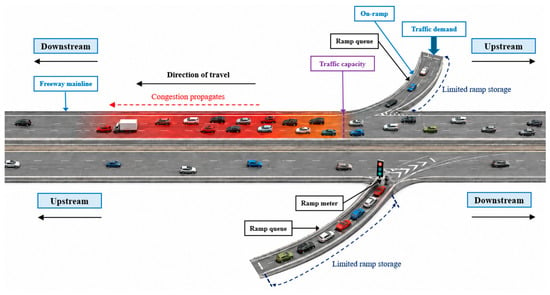
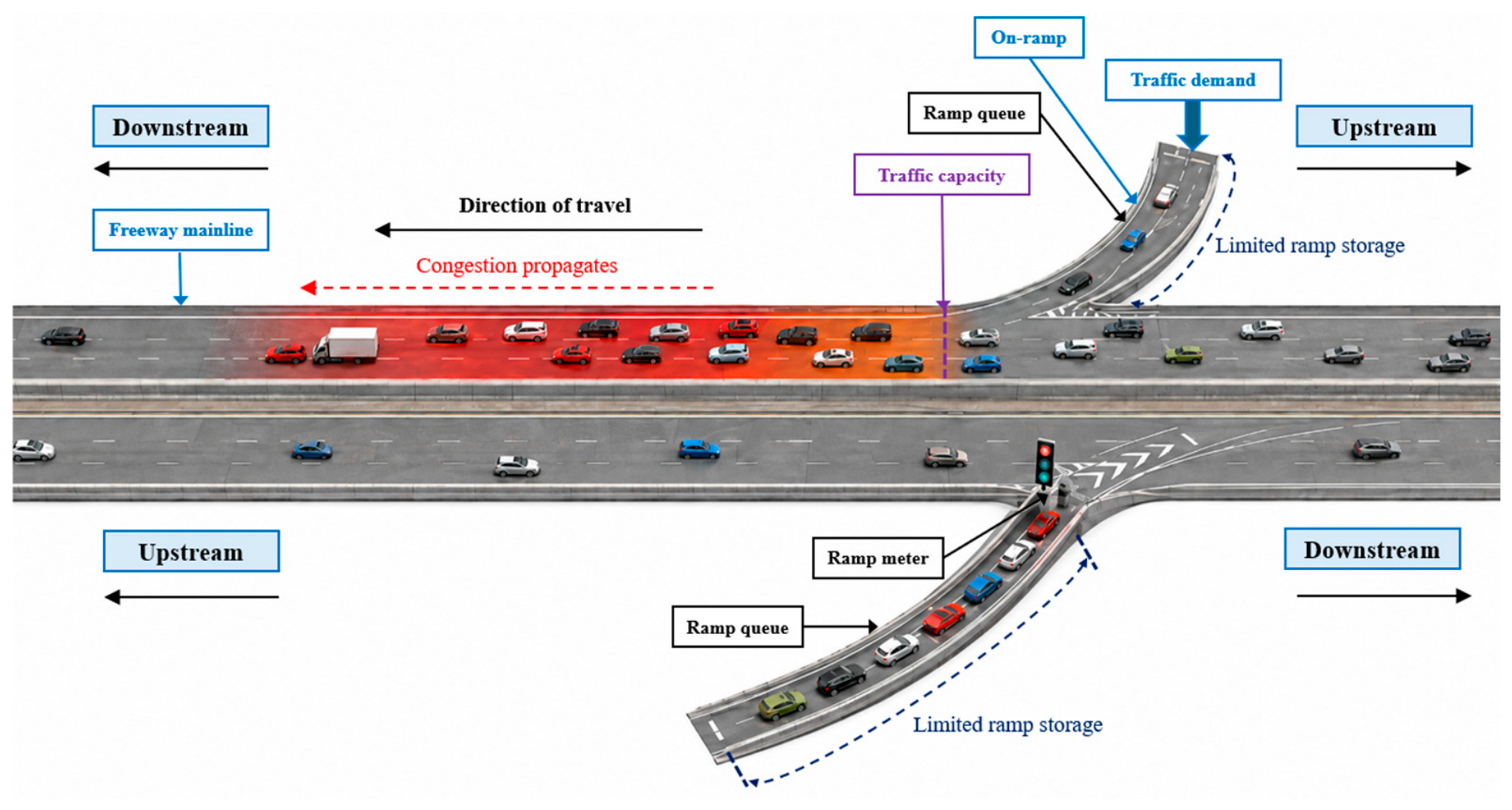
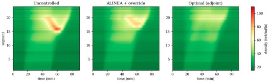
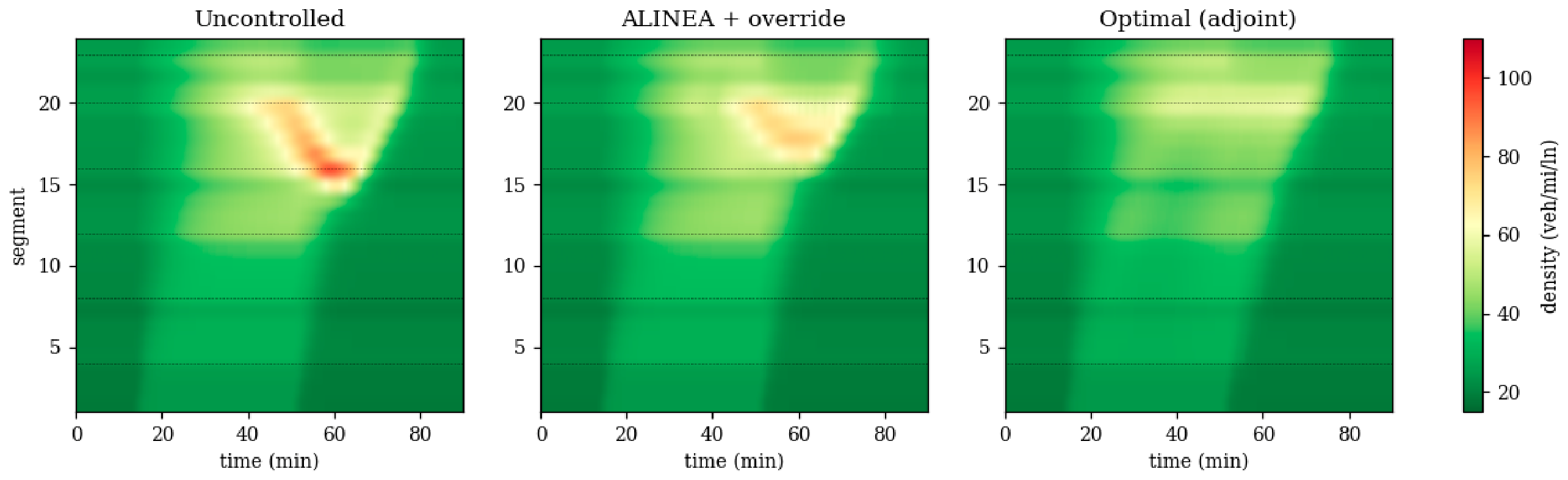
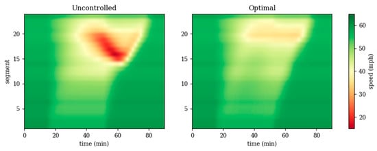
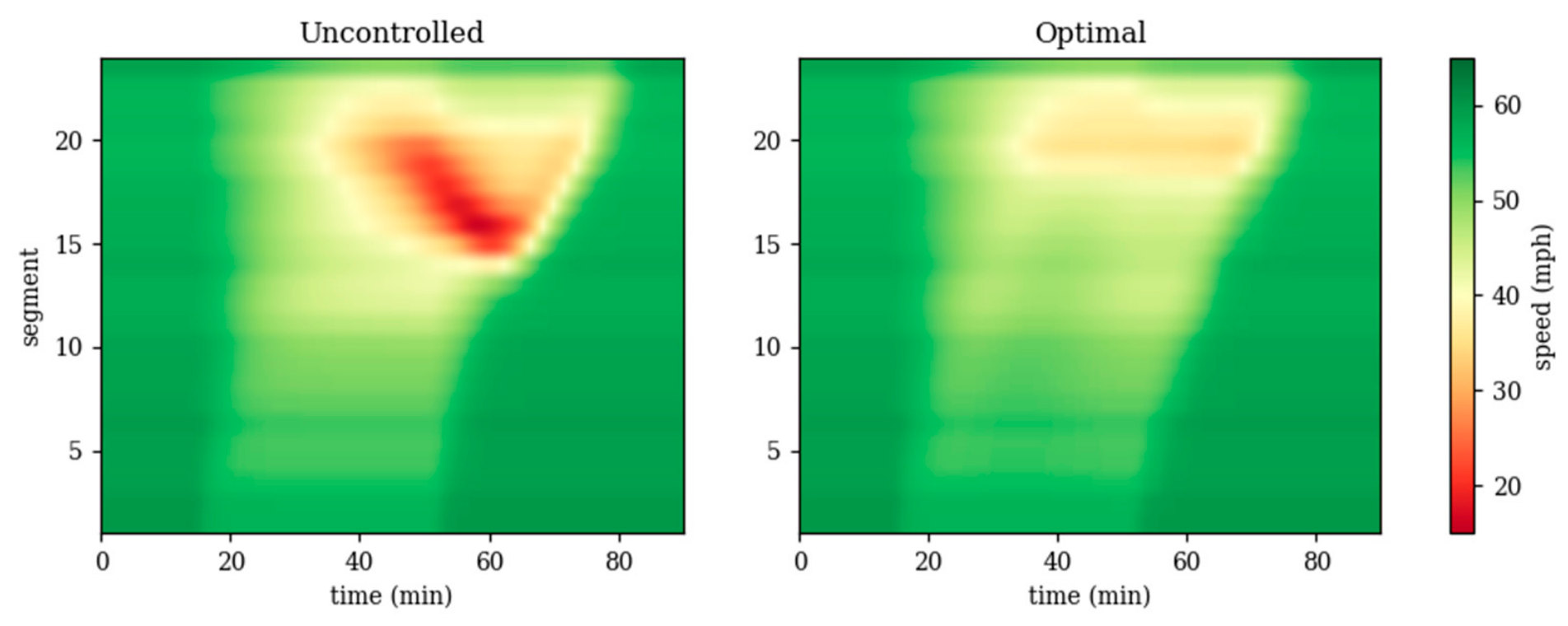
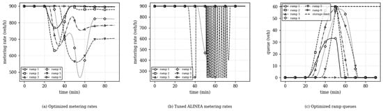
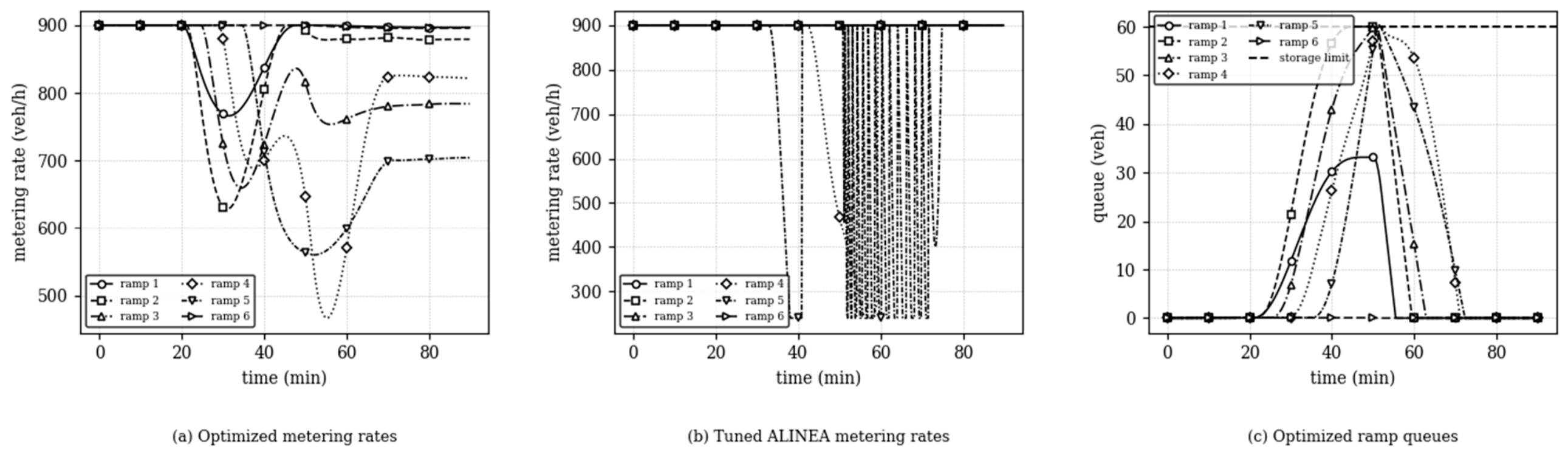
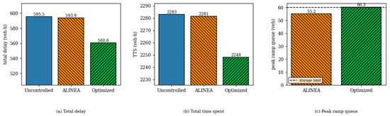
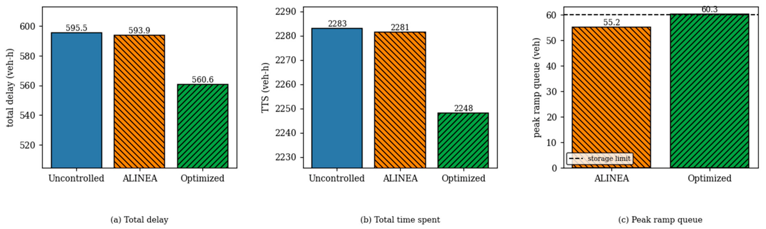
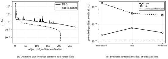
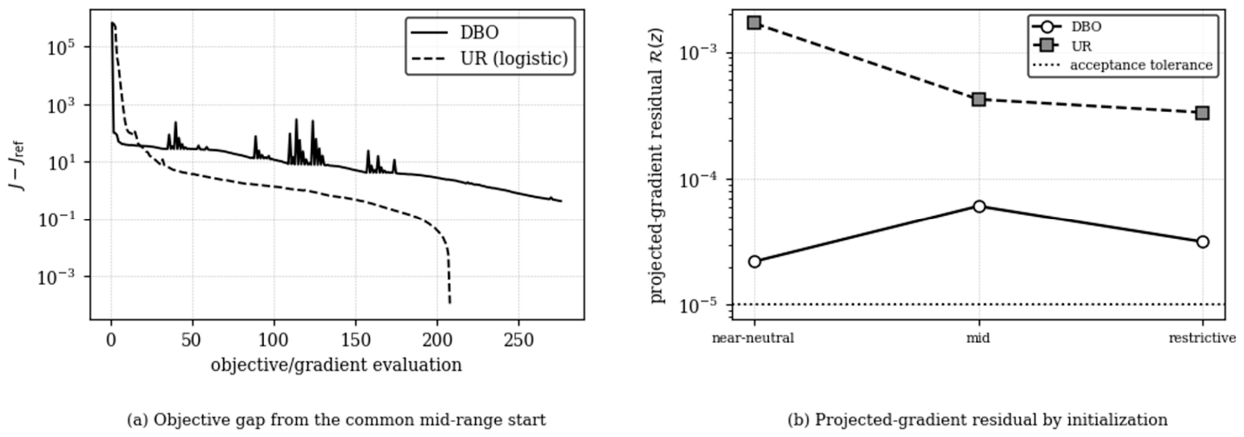
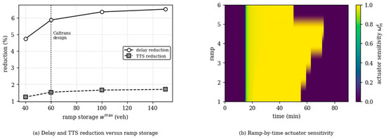
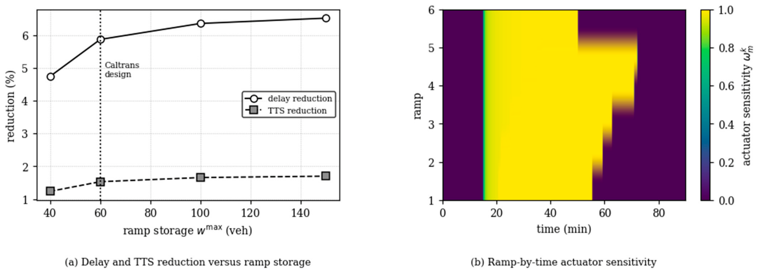
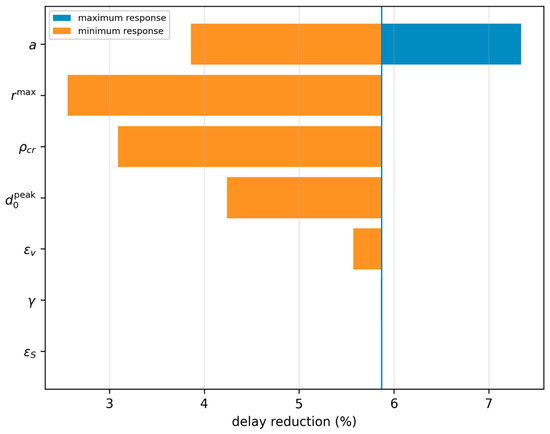
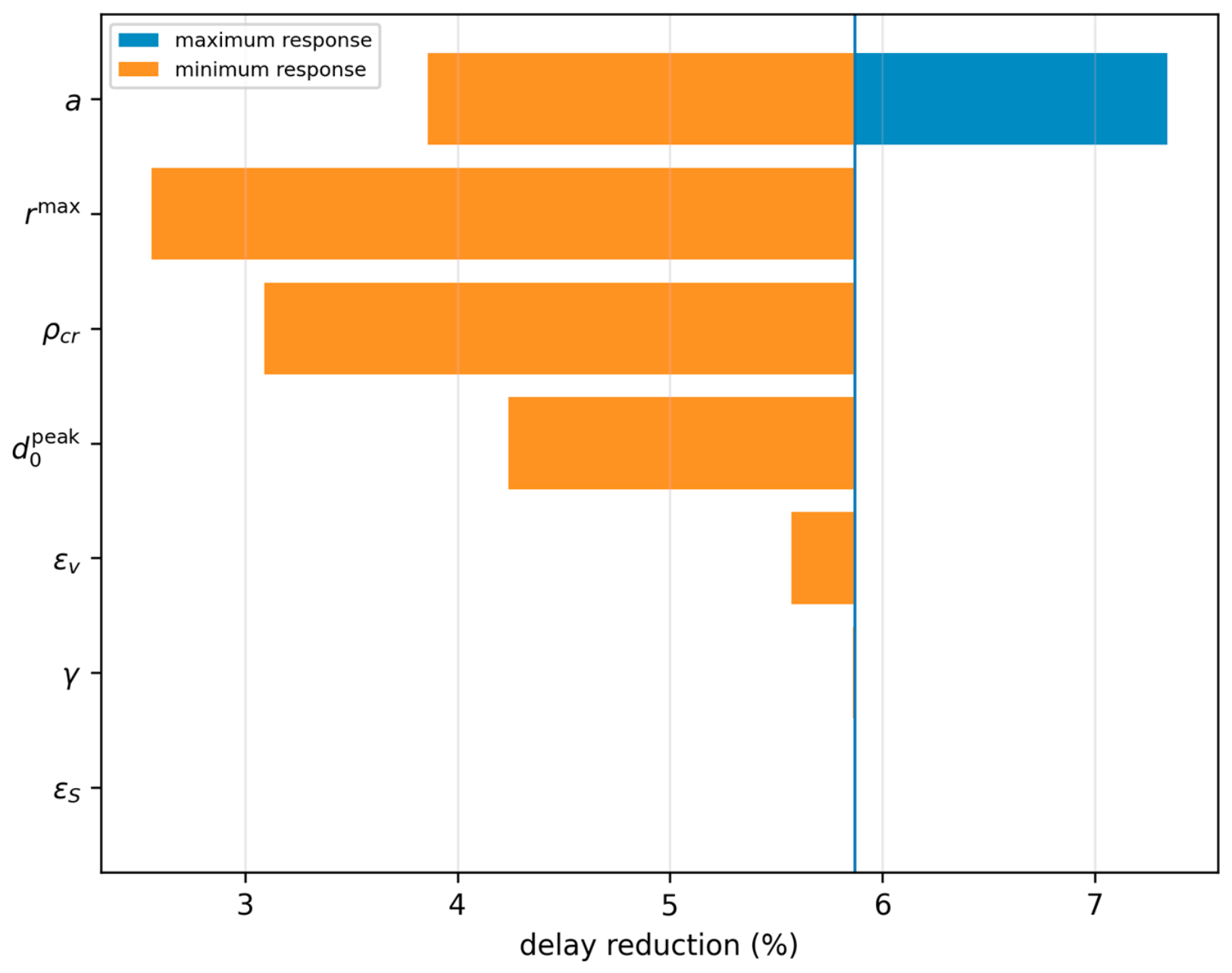
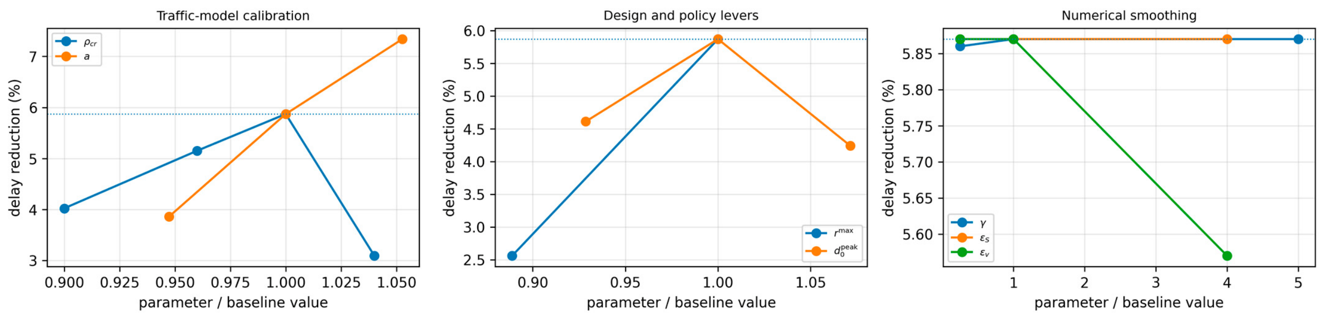
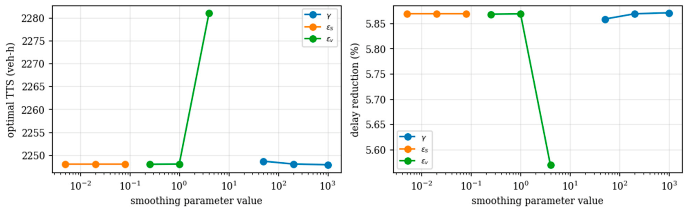

Disclaimer/Publisher’s Note: The statements, opinions and data contained in all publications are solely those of the individual author(s) and contributor(s) and not of MDPI and/or the editor(s). MDPI and/or the editor(s) disclaim responsibility for any injury to people or property resulting from any ideas, methods, instructions or products referred to in the content. |
© 2026 by the authors. Licensee MDPI, Basel, Switzerland. This article is an open access article distributed under the terms and conditions of the Creative Commons Attribution (CC BY) license.