A Non-Traditional Inerter-Based Dynamic Vibration Absorber with Negative Stiffness: Electromechanical Analogies and Optimal Design

Abstract

This paper proposes a non-traditional inerter-based dynamic vibration absorber with negative stiffness (NSIDVA). Its optimal design is determined based on two widely used calibration strategies: the extended fixed-points technique and the stability maximization criterion, each suited respectively to harmonic and transient excitation. The superior performance of the proposed NSIDVA is demonstrated through a comparison with the non-traditional dynamic vibration absorber (DVA) and inerter-based DVA, revealing the benefits of incorporating negative stiffness into mechanical vibration absorbers for enhancing vibration attenuation in both steady-state and transient regimes. Finally, this paper establishes complete electromechanical analogies between piezoelectric shunt dampers and mechanical vibration absorbers (including the proposed NSIDVA), based on which high-performance mechanical vibration absorbers can be realized piezoelectrically, thereby facilitating their implementation in lightweight, space-restricted circumstances.

1. Introduction

The control of mechanical vibrations is of paramount importance in a wide range of engineering applications, including structural engineering, precision manufacturing, aerospace systems and energy harvesting for Internet of Things devices [1,2]. Renowned for its simplicity, efficiency, and reliability, the dynamic vibration absorber (DVA) [3] is a classical device for suppressing mechanical vibrations, with applications reported across a wide range of engineering fields [4,5,6,7]. The classic DVA [3] is a single-degree-of-freedom (SDOF) mass–spring–damper oscillator, in which the absorber mass is connected to the host structure via a spring and a viscous damper in parallel. The non-traditional DVA was first proposed in Ref. [8], in which the absorber mass was supported solely by the spring and linked to the ground through a viscous damper. Compared with the classic DVA, the non-traditional DVA offers marginally better control performance; moreover, it is advantageous when a heavy damper is required or a pendulum-type absorber is to be used. Furthermore, an additional advantage of the non-traditional configuration will be revealed in this paper. To achieve the best possible performance, the parameters of vibration absorbers should be properly tuned according to specific optimization criteria. The first tuning method is the fixed-points technique (FPT) proposed by Den Hartog [3], which approximately minimizes the peak amplitude of the frequency response function (FRF) characterizing the displacement response of the primary system to the excitation force. Clearly, this empirical approach targets the optimization of the steady-state frequency response. To suppress transient vibration in the shortest possible time, however, the absorber should be tuned according to the stability maximization criterion (SMC) [9], which places all poles of the coupled system as far as possible from the imaginary axis in the left half of the complex plane.

To further improve the vibration-control performance of DVA, Hu and Chen [10] replaced the sole damper with a mechanical network comprising a viscous damper, a spring, and an inerter, giving rise to the so-called inerter-based dynamic vibration absorber (IDVA). Herein, it is worth recalling that unlike the mass element, the inerter [11] is a lightweight, two-terminal mechanical element that generates a resisting force proportional to the relative acceleration between its two terminals and enables the establishment of a complete analogy between mechanical and electrical networks. By solving numerically the $H_{\infty }$ and $H_2$ optimization problem of different IDVAs, Hu and Chen [10] showed that, compared with the DVA, the incorporation of inerter-based mechanical networks introduced an additional resonance into the dynamics of the coupled system, yielding a significant improvement in both $H_{\infty }$ and $H_2$ control performance. Later, Barredo et al. [12] extended the classical fixed-point technique to handle the $H_{\infty }$ optimization problem of IDVAs (characterized by four fixed points) and successfully derived closed-form expressions for the optimal parameters. Inspired by the non-traditional DVA, Zhou et al. [13] proposed the non-traditional IDVA, in which the tuned mass is connected to the ground by an inerter-based mechanical network. In this study [13], ready-to-use formulae for the optimal parameters of the non-traditional IDVA were derived using the extended fixed-point technique and the stability maximization criterion, respectively, and the feasibility of realizing the inertial mechanical network via an electromagnetic transducer was also examined. By using a different inerter-based mechanical network, Barredo et al. [14] proposed and investigated another configuration of the non-traditional IDVA. Kendo-Nouja et al. [15] investigated the $H_{\infty }$ and $H_2$ control performance of novel grounded IDVAs. Dogan et al. [16,17,18] numerically and experimentally validated the possibility of using IDVAs to suppress chatter in machine tools so as to increase machining stability.

Another possibility for enhancing the damping efficiency of a DVA is to employ a negative stiffness element in the vibration absorber. Negative stiffness devices originated in the domain of vibration isolation with the objective of addressing the trade-off between the need for high static stiffness and low dynamic stiffness [19,20,21,22]. Unlike these aforementioned devices featuring strong nonlinearity, Acar and Yilmaz [23] conceived a linear negative stiffness mechanism composed of a rigid link and a pre-compressed spring, in which the spring could only deform in a direction perpendicular to the translational DOF of interest. As pointed out in [23], a linear negative stiffness is achieved when the pre-compression of the spring is equal to the length of the rigid link. While in the domain of vibration control, Shen et al. [24] improved the non-traditional DVA by placing a linear negative stiffness between the tuned mass and the ground, numerically proving its significant outperformance compared to the DVA. Later, a thorough analysis of both classical and non-traditional DVAs with negative stiffness was performed by Zhou et al. [9], in which the two aforementioned calibration strategies were employed, and the allowable interval for the magnitude of negative stiffness was clarified in each case. Wang et al. [25] proposed four types of DVAs in conjunction with an inerter and negative stiffness, both grounded, drawing the conclusion that the simultaneous use of an inerter and negative stiffness does enhance the vibration-control performance of all four DVAs, while finding that their contribution cannot be simply superposed in the cases where the damper of the DVA is grounded. Research has also been devoted to using negative stiffness to enhance the vibration-isolation performance of tuned inerter dampers [26,27], the vibration mitigation of cables [28,29] and the vibration-control performance of passive dampers [30,31].

Despite the aforementioned advances, several research gaps remain to be addressed. First, while the inerter and negative stiffness have each been shown to enhance the performance of DVAs, their combined effect in the non-traditional configuration has not been systematically investigated through analytical optimization. Second, existing electromechanical analogies are limited to traditional configurations where a physical tuned mass is still required, constraining their applicability in lightweight and space-restricted scenarios. Third, the non-traditional configuration, which places the dissipative mechanism between the tuned mass and the ground, offers a unique advantage in establishing complete electromechanical analogies, yet this potential remains unexplored. The present work aims to fill these gaps.

This present paper will propose a vibration absorber, referred to as the non-traditional IDVA with negative stiffness (NSIDVA), in which both the inerter-based mechanical network and the linear negative stiffness are positioned between the tuned mass and the ground. The optimal design of the NSIDVA is determined according to the extended fixed-point technique and the stability maximization criterion, respectively. Such a device is expected to combine the benefits of both mechanical components and to exhibit superior control performance. In addition, existing studies on electromechanical analogies have focused on replacing parts of mechanical absorbers with electromechanical shunt circuits to replicate similar dynamics [32,33,34]; however, a physical tuned mass is still required in such devices, so their applications remain limited by physical constraints such as mass and space. To address this issue, another main contribution of this paper is to show that mechanical absorbers with a non-traditional configuration—i.e., with the dissipative mechanism placed between the tuned mass and the ground—can be mapped onto piezoelectric shunt circuits in a completely analogous manner. It is worth mentioning that, in this context, piezoelectric shunt dampers exactly equivalent to some existing or newly proposed inerter-involved mechanical devices could be designed. This is of great interest, since a mechanical model can be validated by testing its analogous shunt damper, and, conversely, the development of higher-performance mechanical absorbers can inspire the design of more efficient shunt circuits.

To the best of the authors’ knowledge, the present work differs from prior studies in the following three fundamental aspects: First, although Wang et al. [25] investigated four types of DVAs with the inerter and negative stiffness both grounded, the analytical optimization (including the derivation of closed-form expressions for all tuning parameters) of the non-traditional IDVA configuration C3 with simultaneous grounded inerter-based network and negative stiffness has not been reported. Second, the non-traditional configuration, in which the dissipative mechanism is placed between the tuned mass and the ground, enables a complete electromechanical analogy that cannot be achieved by the traditional configuration. Third, this paper establishes a comprehensive table of electromechanical analogies covering both existing absorbers and the newly proposed NSIDVA, providing a theoretical basis for piezoelectric realization.

This paper is organized as follows: The next section formulates the mathematical model of an SDOF primary system coupled with the proposed NSIDVA and establishes the electromechanical analogies. In Section 3, the parameters of the NSIDVA are optimally tuned according to the two calibration strategies in turn. Section 4 presents numerical simulations and analyses comparing the three mechanical absorbers and examining the effect of negative stiffness on vibration-control performance. Finally, the main conclusions of this study are drawn in Section 5.

2. Mathematical Modelling and Electromechanical Analogy

2.1. Description of Proposed NSIDVA

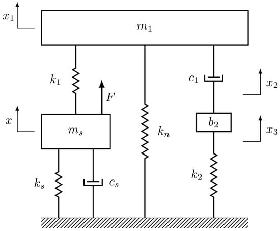
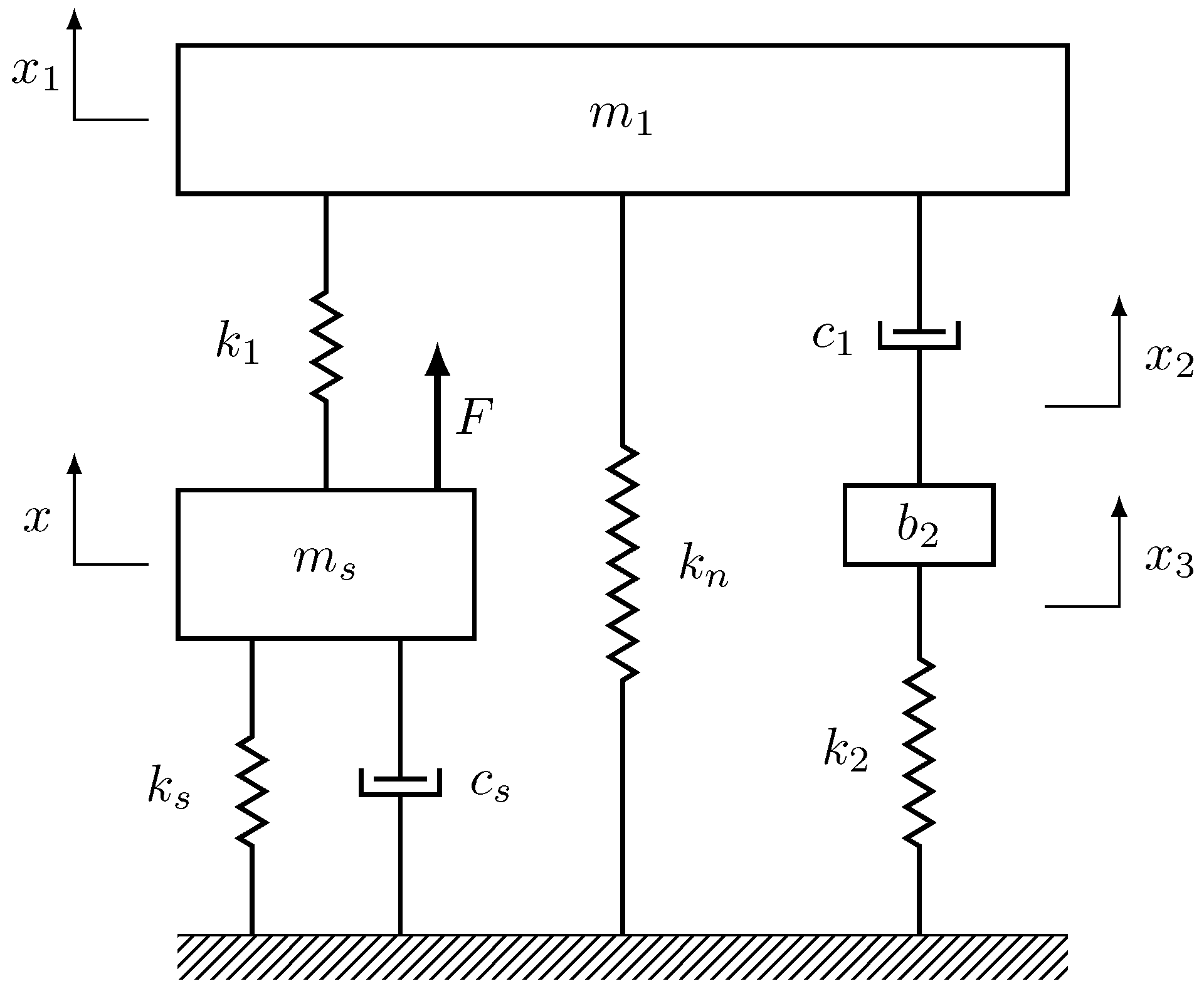
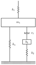
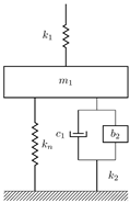
Figure 1 shows an SDOF primary system controlled by the proposed NSIDVA under direct force excitation. The mass, damping coefficient, and stiffness of the primary system are denoted $m_s$, $c_s$ and $k_s$, respectively. The tuned mass $m_1$ is mounted on the primary system by the supporting spring $k_1$ and is linked to the ground by the negative stiffness $k_n$ and the inerter-based mechanical network, which is a series connection of the damper $c_1$, the inerter $b_2$ and the spring $k_2$.

Figure 1. Mechanical model of an SDOF primary system coupled with the proposed NSIDVA under direct force excitation.

It is worth noting that the damper $c_1$, the inerter $b_2$, and the spring $k_2$ are connected in series, forming a Maxwell-type inerter network. This series configuration is adopted for the following reasons: First, unlike a parallel arrangement, the series connection introduces additional internal degrees of freedom (characterized by the displacements $x_2$ and $x_3$), thereby extending the coupled system from 2 DOFs to 3 DOFs and generating an additional resonance peak that broadens the effective vibration suppression bandwidth. Second, this configuration follows the IDVA-C3 design proposed by Hu and Chen [10], which has been shown to achieve superior $H_{\infty }$ and $H_2$ control performance compared with traditional parallel configurations. Third, the impedance structure of the series network is amenable to both analytical optimization and piezoelectric shunt circuit realization.

In practice, the linear negative stiffness element $k_n$ can be realized through several mechanisms. The rigid link and pre-compressed spring mechanism proposed by Acar and Yilmaz [23] provide a compact, linear negative stiffness when the spring pre-compression equals the length of the rigid link. Alternatively, bistable beam and compliant constant-force mechanisms can also generate negative stiffness, as demonstrated in the context of quasi-zero-stiffness isolators [35]. The magnitude of negative stiffness can be adjusted by varying the spring pre-compression or the geometric parameters of the mechanism, enabling the practical tuning of the negative stiffness ratio to match the optimal design.

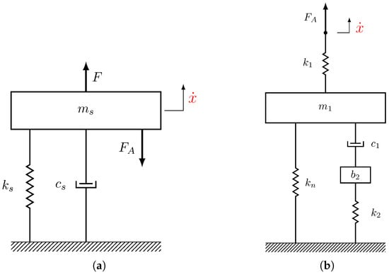
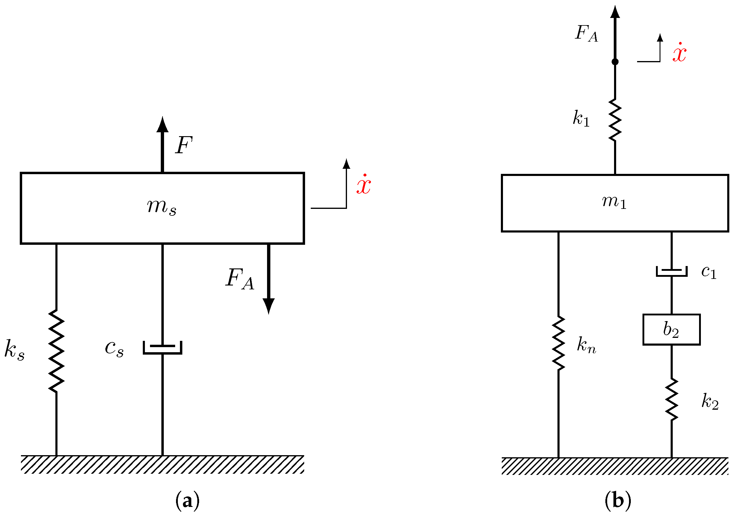
Owing to the non-traditional configuration, the structure in question can be partitioned into two substructures, namely the primary system in Figure 2a and the absorber in Figure 2b, which share the same velocity at their two extremities. Therefore, the overall dynamics of the coupled system could be expressed as:

$$\begin{array}{c}\hfill Z_s·\dot{x}+F_A=F\end{array}$$

(1)

where $\dot{x}$ is the velocity common across the two substructures, where the dot over the symbol denotes differentiation with respect to time t. In addition, $Z_s=m_{s}s+c_s+k_s/s$ stands for the structural impedance of the primary system, where $s=j\omega$ is the Laplace variable, $\omega$ is the angular frequency and $j=\sqrt{-1}$. Finally, $F_A=Z_A·\dot{x}$ is the resisting force exerted by the mechanical absorber with $Z_A$ being its structural impedance. For the NSIDVA, $Z_A$ can be easily formulated according to the addition laws of mechanical impedances:

$$Z_A^{-1}={\displaystyle \frac{s}{k_1}}+{\displaystyle \frac{1}{m_{1}s+{\displaystyle \frac{k_n}{s}}+{\displaystyle \frac{1}{{\displaystyle \frac{1}{c_1}}+{\displaystyle \frac{s}{k_2}}+{\displaystyle \frac{1}{b_{2}s}}}}}}$$

(2)

To mimic the dynamics of the proposed NSIDVA, the piezoelectric shunt damper should lead to the same form of governing Equations (1) and (2), which will be discussed in the next subsection.

Figure 2. Partition of coupled system in question: (a) host structure and (b) mechanical absorber. Two substructures have same velocities at two extremities.

2.2. Equivalent Piezoelectric Shunt Damper

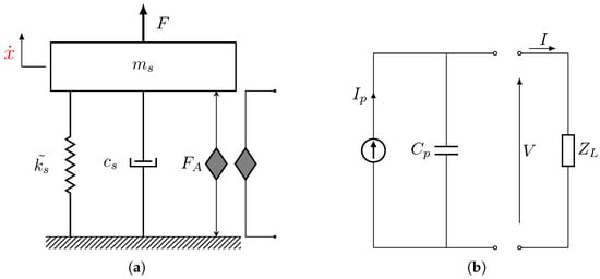
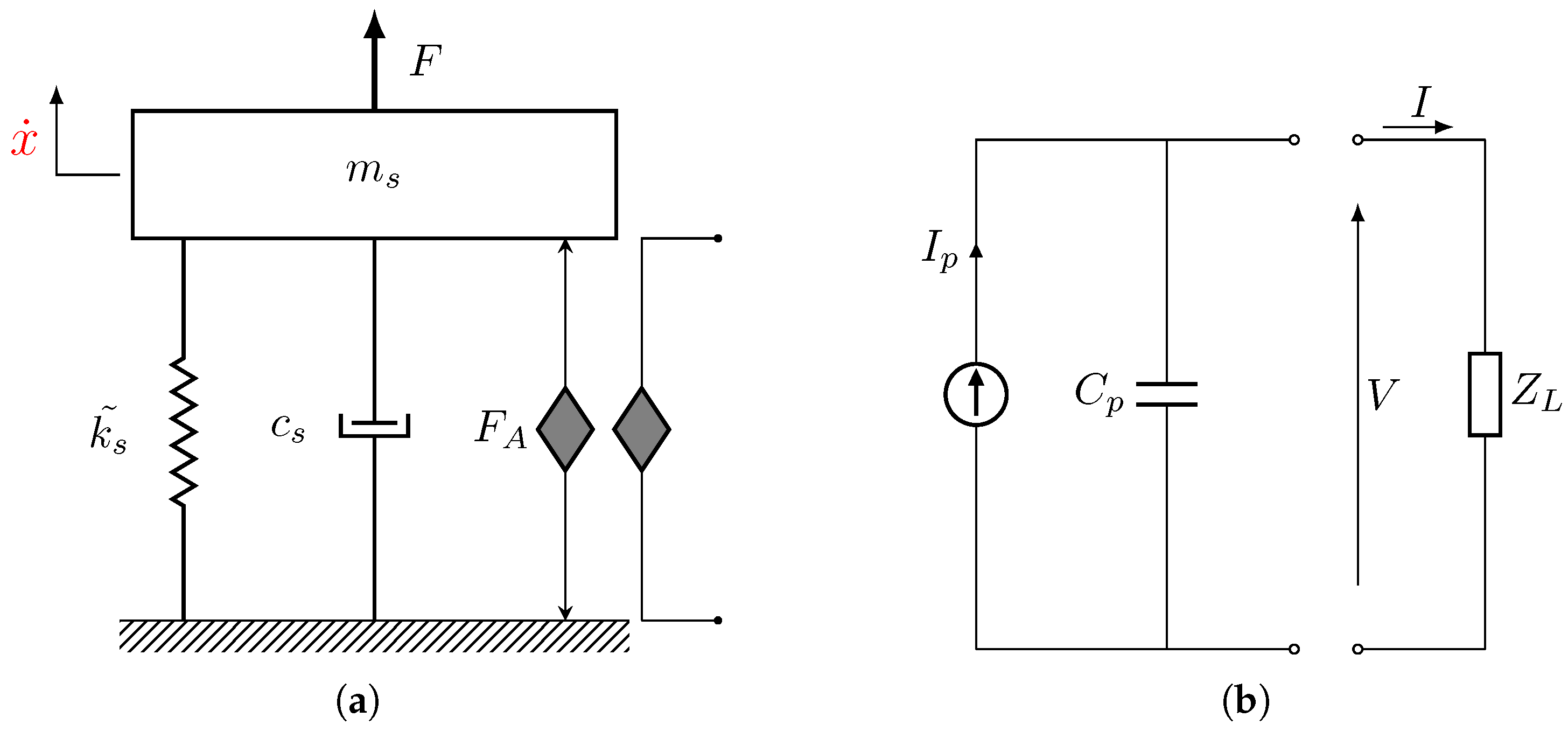
Let us consider the SDOF primary system being controlled by a piezoelectric shunt damper, as shown in Figure 3a. The equivalent circuit representation of the shunted piezoelectric is schematized in Figure 3b, where the piezoelectric transducer is modelled as a current source $I_p$ and $Z_L$ is the general electrical impedance.

Figure 3. (a) Mechanical model of an SDOF primary system controlled by a piezoelectric shunt damper. (b) The equivalent circuit representation of the piezoelectric shunt damper enclosed by a general electrical impedance $Z_L$.

The equivalent circuits are presented alongside the mechanical models to demonstrate the one-to-one correspondence between the non-traditional mechanical absorbers and their piezoelectric shunt counterparts. This complete electromechanical analogy constitutes a core contribution of this paper, as it establishes that mechanical absorbers with a non-traditional configuration can be fully synthesized by piezoelectric shunt circuits without the need for a physical tuned mass, thereby facilitating practical applications in scenarios subject to mass and space constraints.

The dynamics of the electromechanical system can be governed by the equations of motion [36]:

$$\begin{array}{cc}\hfill \widetilde{Z_s}·\dot{x}+F_A& =F\hfill \\ \hfill \left(I_p-C_{p}s·V\right)·Z_L& =V\hfill \end{array}$$

(3)

with

$$\begin{array}{cccc}\hfill F_A& =\varphi ·V,\hfill & \hfill I_p& =\varphi ·\dot{x}.\hfill \end{array}$$

(4)

where $\widetilde{Z_s}=m_{s}s+c_s+\widetilde{k_s}/s$ and $\widetilde{k_s}=k_s+k_p$ is the total mechanical stiffness of the primary system and piezoelectric transducer. $\varphi$ is the electromechanical coupling factor of the piezoelectric element and $C_p$ refers to its inherent capacitance. Then, Equation (3) can be alternatively expressed as:

$$\widetilde{Z_s}·\dot{x}+{\displaystyle \frac{{\varphi }^2}{C_{p}s+Z_L^{-1}}}·\dot{x}=F$$

(5)

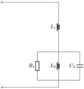
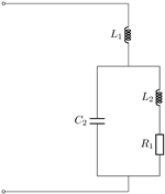
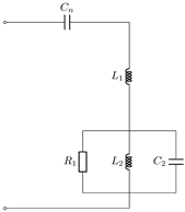
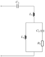
To establish a completely analogous relationship, it is evident upon inspection of Equations (1), (2) and (5) that the piezoelectric capacitance $C_p$ is analogous to the reciprocal of the mechanical stiffness $k_1$ of NSIDVA. Moreover, the general electrical load should be formulated as:

$$Z_L=L_{1}s+{\displaystyle \frac{1}{C_{n}s}}+{\displaystyle \frac{1}{{\displaystyle \frac{1}{R_1}}+C_{2}s+{\displaystyle \frac{1}{L_{2}s}}}}$$

(6)

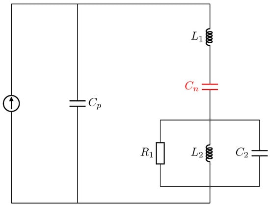
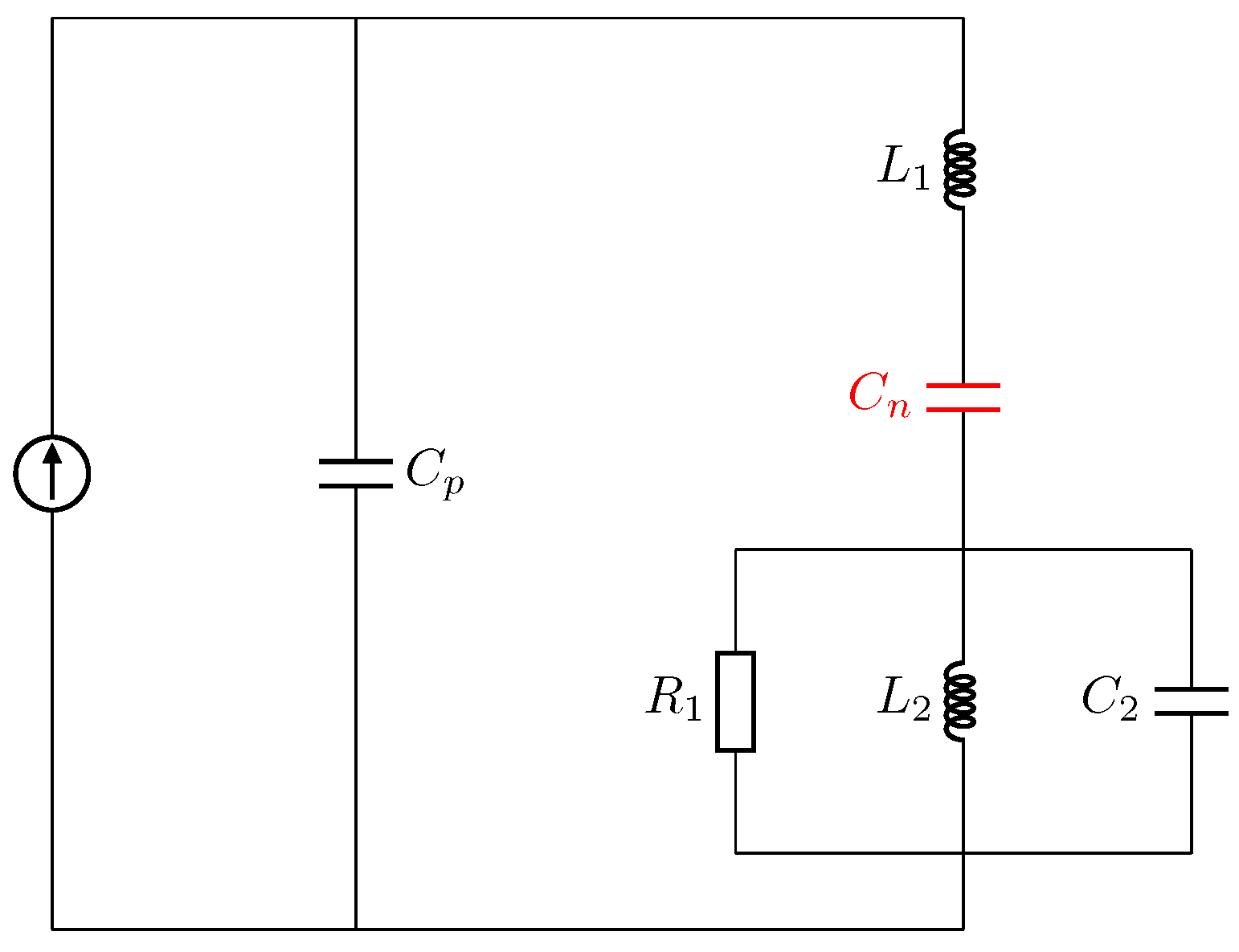
According to the addition laws of electrical impedances, the external shunt $Z_L$ should be an inductor $L_1$ and a negative capacitor $C_n$ in series, which is further joined by the parallel connection of a resistor $R_1$, a capacitor $C_2$ and an inductor $L_2$, as shown in Figure 4. Meanwhile, the electrical components are related to their equivalent mechanical quantities by:

$$\begin{array}{cccccc}\hfill L_1& ={\displaystyle \frac{m_1}{{\varphi }^2}},\hfill & \hfill L_2& ={\displaystyle \frac{b_2}{{\varphi }^2}},\hfill & \hfill R_1& ={\displaystyle \frac{c_1}{{\varphi }^2}},\hfill \\ \hfill C_p& ={\displaystyle \frac{{\varphi }^2}{k_1}},\hfill & \hfill C_2& ={\displaystyle \frac{{\varphi }^2}{k_2}},\hfill & \hfill C_n& ={\displaystyle \frac{{\varphi }^2}{k_n}}.\hfill \end{array}$$

(7)

Figure 4. The piezoelectric shunt circuit completely analogous to the NSIDVA.

Clearly, one may purposely add an additional capacitance in parallel with the transducer so as to achieve the required amount of equivalent stiffness. Finally, it should be noted that, in the case of an electromechanical system, the natural frequency is altered by the presence of the piezoelectric element, which should be taken into consideration.

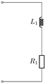
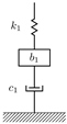
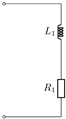
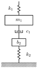
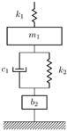
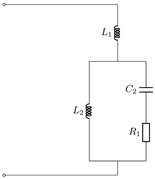
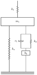
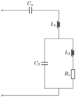
Following the same procedure, electrical analogues of four types of mechanical devices have been identified, as summarized in Table 1. First, the Maxwell damper can be realized by a resistively shunted piezoelectric; meanwhile, the non-traditional DVA of Ren [8] could be paralleled by the series resistive–inductive (RL) shunt, which has also been noted by Gripp and Rade [37]. Furthermore, the parallel and series RL shunt circuits are exactly equivalent to the inerter-based isolators of types C4 and C5 developed by Hu et al. [38], respectively. Finally, further insight can be gained by comparing the non-traditional DVA with the inerter-based isolator of type C5. As is evident from Table 1, these two devices are equivalent from the perspective of their electrical analogue. In other words, they exhibit the same vibration-control or isolation performance when the tuned mass $m_1$ is equal to the inertance $b_1$. Nevertheless, the advantage claimed for the inerter-based isolator over the non-traditional DVA lies in the fact that the inerter can generate an inertance up to two orders of magnitude larger than its physical mass [39]. Thus, the inerter-based isolator is preferable for lightweight applications.

Table 1. Piezoelectric shunt circuits exactly equivalent to the Maxwell damper, the non-traditional DVA and two types of inerter-based isolators developed in Ref. [38].

	Mechanical Model	Equivalent Piezoelectric Shunt
Maxwell damper
Non-traditional DVA
Inerter-based isolator (type C4 in Ref. [38])
Inerter-based isolator (type C5 in Ref. [38])

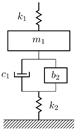
Table 2 provides the equivalent piezoelectric shunt dampers of three types of IDVAs. These mechanical devices are in fact the non-traditional versions of the IDVAs proposed by Hu and Chen [10] (of types C3, C4 and C6, respectively). It can be inferred that, when properly tuned, these high-order shunt circuits are more effective than the commonly used series or parallel RL shunts. Finally, an observation can be made in conjunction with Figure 4 and Table 2 that the negative stiffness $k_n$ relating the tuned mass to the ground can be realized in an analogous manner by adding a negative capacitance $C_n$ in the main branch, i.e., in series with the inductance $L_1$. In this way, the piezoelectric shunt dampers equivalent to three types of NSIDVAs with the non-traditional configuration are summarized in Table 3.

Table 2. Piezoelectric shunt circuits exactly equivalent to three types of non-traditional IDVAs (with the designations of C3, C4 and C6, originating from Ref. [10]).

	Mechanical Model	Equivalent Piezoelectric Shunt
IDVA-C3
IDVA-C4
IDVA-C6

Table 3. Piezoelectric shunt circuits exactly equivalent to three types of non-traditional IDVAs with negative stiffness (with the designations of C3, C4 and C6, originating from Ref. [10]).

	Mechanical Model	Equivalent Piezoelectric Shunt
NSIDVA-C3
NSIDVA-C4
NSIDVA-C6

It should be clarified that Table 1, Table 2 and Table 3 are not intended for performance comparison among the different absorber configurations. Rather, their purpose is to establish a complete electromechanical analogy between various mechanical vibration absorbers (including existing devices and the newly proposed NSIDVA) and their equivalent piezoelectric shunt circuits. This analogy serves two purposes: (1) it enables the validation of mechanical models through electrical circuit experiments, and (2) it provides theoretical guidance for realizing high-performance mechanical absorbers as lightweight piezoelectric shunt dampers suitable for space-constrained applications.

In this paper, the type C3 NSIDVA is selected for in-depth investigation for the following reasons: First, the series connection of the damper, inerter, and spring in the C3 configuration yields a Maxwell-type inerter network whose impedance structure is amenable to both the extended fixed-point technique and the stability maximization criterion, each yielding closed-form solutions. Second, the C3 configuration is the most widely studied non-traditional IDVA in the literature [10,13], facilitating direct and fair comparison with existing results. Third, the characteristic equations of the C4 and C6 configurations exhibit different structural forms, and the direct application of the present analytical optimization procedure to these configurations encounters technical challenges that require separate treatment, which is left for future research.

2.3. Dimensionless Equations of Motion

In an effort to derive closed-form solutions for tuning parameters, zero damping is necessarily assumed for the host structure, i.e., $c_s=0$. Therefore, the overall dynamics of the system in Figure 1 should be governed by:

$$\begin{array}{cc}\hfill m_s\ddot{x}+k_{s}x+k_1(x-x_1)& =F\left(t\right)\hfill \end{array}$$

(8a)

$$\begin{array}{cc}\hfill m_1{\ddot{x}}_1+c_1({\dot{x}}_1-{\dot{x}}_2)+k_1(x_1-x)+k_n{x}_1& =0\hfill \end{array}$$

(8b)

$$\begin{array}{cc}\hfill b_2({\ddot{x}}_3-{\ddot{x}}_2)+c_1({\dot{x}}_1-{\dot{x}}_2)& =0\hfill \end{array}$$

(8c)

$$\begin{array}{cc}\hfill b_2({\ddot{x}}_2-{\ddot{x}}_3)-k_2{x}_3& =0\hfill \end{array}$$

(8d)

where $x_1$, $x_2$ and $x_3$ are the displacements of absorber mass $m_1$ and those at upper and lower terminals of inerter $b_2$, respectively. To facilitate the analytical optimization, dimensionless parameters are introduced as follows:

$$\begin{array}{cccccccccccc}\hfill \mu & ={\displaystyle \frac{m_1}{m_s}},\hfill & \hfill \nu & ={\displaystyle \frac{b_2}{m_s}},\hfill & \hfill \xi & ={\displaystyle \frac{c_1}{2\sqrt{k_1{m}_1}}},\hfill & \hfill \alpha & ={\displaystyle \frac{{\omega }_1}{{\omega }_s}},\hfill & \hfill \beta & ={\displaystyle \frac{{\omega }_2}{{\omega }_s}},\hfill & \eta & ={\displaystyle \frac{k_n}{k_s}}.\end{array}$$

(9)

with $\eta \le 0$ and the definition of three natural frequencies given by:

$$\begin{array}{cccccc}\hfill {\omega }_s& =\sqrt{{\displaystyle \frac{k_s}{m_s}}},\hfill & \hfill {\omega }_1& =\sqrt{{\displaystyle \frac{k_1}{m_1}}},\hfill & \hfill {\omega }_2& =\sqrt{{\displaystyle \frac{k_2}{b_2}}}.\hfill \end{array}$$

(10)

In this study, the mass ratio $\mu$ and the negative stiffness ratio $\eta$ are user-defined parameters; therefore, one aims to find the optimal values of the inertance-to-mass ratio $\nu$, mechanical damping ratio $\xi$ and frequency tuning ratios $\alpha$ and $\beta$ as a function of $\mu$ and $\eta$. By rescaling the time t by ${\omega }_s$, i.e., $\tau ={\omega }_{s}t$, the equations of motion (8) are transformed into:

$$\begin{array}{cc}\hfill x^{″}+x+\mu {\alpha }^2(x-x_1)& =F\left(\tau \right)/k_s\hfill \end{array}$$

(11a)

$$\begin{array}{cc}\hfill \mu x_1^{″}+2\xi \mu \alpha (x_1^{\prime }-x_2^{\prime })+\mu {\alpha }^2(x_1-x)+\eta x_1& =0\hfill \end{array}$$

(11b)

$$\begin{array}{cc}\hfill \nu (x_3^{″}-x_2^{″})+2\xi \mu \alpha (x_1^{\prime }-x_2^{\prime })& =0\hfill \end{array}$$

(11c)

$$\begin{array}{cc}\hfill x_2^{″}-x_3^{″}-{\beta }^2{x}_3& =0\hfill \end{array}$$

(11d)

where the prime indicates differentiation with respect to the rescaled time $\tau$. Denoting the complex magnitudes of x and $F\left(\tau \right)$ by X and F, the FRF from the static deformation to the displacement of the primary system has the form of:

$${\displaystyle \frac{X}{F/k_s}}={\displaystyle \frac{N_4{\overline{s}}^4+N_3{\overline{s}}^3+N_2{\overline{s}}^2+N_1\overline{s}+N_0}{D_6{\overline{s}}^6+D_5{\overline{s}}^5+D_4{\overline{s}}^4+D_3{\overline{s}}^3+D_2{\overline{s}}^2+D_1\overline{s}+D_0}}$$

(12)

where $\overline{s}=j\omega /{\omega }_s$, and the coefficients of its numerator and denominator are given in Appendix A.

3. Analytical Optimization of NSIDVA

In this section, the parameters of the NSIDVA are optimized with the objective of minimizing the peak amplitude of the displacement FRF and the decay time of the transient response. Therefore, the optimal design is determined according to the extended fixed-point technique and the stability maximization criterion, respectively.

The FPT and SMC are analytical optimization methods that provide closed-form expressions for all tuning parameters, which facilitate parametric design, sensitivity analysis, and physical interpretation of the results. While data-driven approaches such as machine learning offer complementary advantages for complex nonlinear systems, the analytical nature of the present methods ensures the transparency and generalizability of the optimal design.

3.1. Calibration Based on the Extended Fixed-Points Technique

By substituting $\overline{s}=j\lambda$ into Equation (12), the displacement amplitude of the primary system normalized by its static displacement can be retrieved as:

$$\begin{array}{ccc}\hfill G\left(\lambda \right)& =\left|{\displaystyle \frac{X}{F/k_s}}\right|\hfill & \hfill =\sqrt{{\displaystyle \frac{4{\xi }^2·A(\lambda ,\mu ,\eta ,\nu ,\alpha ,\beta )+B(\lambda ,\mu ,\eta ,\nu ,\alpha ,\beta )}{4{\xi }^2·C(\lambda ,\mu ,\eta ,\nu ,\alpha ,\beta )+D(\lambda ,\mu ,\eta ,\nu ,\alpha ,\beta )}}}\end{array}$$

(13)

where $\lambda =\omega /{\omega }_s$ is the frequency of excitation force $F\left(t\right)$ normalized by the natural frequency of the host structure, while expressions of functions, $A(\lambda ,\mu ,\eta ,\nu ,\alpha ,\beta )$, $B(\lambda ,\mu ,\eta ,\nu ,\alpha ,\beta )$, $C(\lambda ,\mu ,\eta ,\nu ,\alpha ,\beta )$ and $D(\lambda ,\mu ,\eta ,\nu ,\alpha ,\beta )$, can be found in Appendix A.

3.1.1. Optimal Values of $\nu$, $\alpha$ and $\beta$

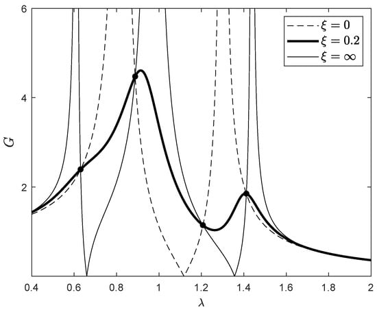
As shown in Figure 5, the frequency response curves under different damping levels always intersect at four invariant positions. Thus, one may locate these fixed points by equating the vibration amplitudes of the primary system under different damping levels, and an efficient and classical approach is to consider two extreme cases, i.e., $\xi =0$ and $\xi \to \infty$. In this way, one has

$$G{|}_{\xi =0}=\sqrt{{\displaystyle \frac{B}{D}}}=\sqrt{{\displaystyle \frac{A}{C}}}=G{|}_{\xi \to \infty }$$

(14)

yielding a fourth-order polynomial in ${\lambda }^2$:

$${\displaystyle \sum _{k=0}^4}{a}_k(\mu ,\eta ,\nu ,\alpha ,\beta )·{\left({\lambda }^2\right)}^k=0$$

(15)

To achieve more equality conditions, one may intentionally introduce a new variable h which designates the square of vibration amplitude at fixed points, i.e., $h=G^2{|}_{\xi =0}=G^2{|}_{\xi \to \infty }$. Subsequently, another fourth-order polynomial in ${\lambda }^2$ could be obtained:

$${\displaystyle \sum _{k=0}^4}{b}_k(\mu ,\eta ,\nu ,\alpha ,\beta ,h)·{\left({\lambda }^2\right)}^k=0$$

(16)

The coefficients before the terms in Equations (15) and (16) are both detailed in Appendix A. In order to yield the same group of fixed points, the coefficients related to the like power of ${\lambda }^2$, $a_k$ and $b_k$ with $k=0,\dots ,3$ should be constrained by the following relationship:

$${\displaystyle \frac{a_k}{a_4}}={\displaystyle \frac{b_k}{b_4}},k=0,\dots ,3.$$

(17)

At this point, one has four equality conditions associated with four variables, i.e., $\nu$, $\alpha$, $\beta$ and h. The combination of all four conditions cumulates into a quadratic equation solely in terms of ${\alpha }^2$ as follows:

$${\mu }^2{\alpha }^4+(2\eta \mu -\eta {\mu }^2-{\mu }^2){\alpha }^2+{\eta }^2-\eta \mu =0$$

(18)

from which two possible solutions for $\alpha$ could exist:

$$\begin{array}{cccc}\hfill {\alpha }_1& =\sqrt{{\displaystyle \frac{\mu (1+\eta )-2\eta -\sqrt{{\mu }^2{(1+\eta )}^2-4\mu {\eta }^2}}{2\mu }}},\hfill & \hfill {\alpha }_2& =\sqrt{{\displaystyle \frac{\mu (1+\eta )-2\eta +\sqrt{{\mu }^2{(1+\eta )}^2-4\mu {\eta }^2}}{2\mu }}}.\hfill \end{array}$$

(19)

It is apparent that when the negative stiffness is removed, i.e., $\eta =0$, ${\alpha }_1$ will reduce to zero while ${\alpha }_2$ will be equal to unity. Thus, the second possible solution should be retained as the optimal frequency tuning ratio ${\alpha }_{\mathrm{fpt}}$, namely:

$${\alpha }_{\mathrm{fpt}}=\sqrt{{\displaystyle \frac{\mu (1+\eta )-2\eta +\sqrt{{\mu }^2{(1+\eta )}^2-4\mu {\eta }^2}}{2\mu }}}$$

(20)

Meanwhile, the optimal inertance-to-mass ratio ${\nu }_{\mathrm{fpt}}$ can be formulated as a function of $\alpha$ in such a way that:

$${\nu }_{\mathrm{fpt}}={\displaystyle \frac{2{\mu }^3{\alpha }^4\left[(\mu -{\mu }^2){\alpha }^2+\eta -\mu \right]}{{\mu }^4{\alpha }^6-(2\mu \eta -2\eta +\mu -2){\mu }^2{\alpha }^4+2\mu ({\eta }^2-2\mu \eta +2\eta -\mu ){\alpha }^2+2{\eta }^2-2\mu \eta }}$$

(21)

Similarly, the optimal frequency tuning ratio ${\beta }_{\mathrm{fpt}}$ is obtained with the knowledge of $\alpha$ and $\nu$:

$${\beta }_{\mathrm{fpt}}=\sqrt{{\displaystyle \frac{\mu +{\mu }^2{\alpha }^2}{\mu +\nu }}}$$

(22)

Finally, the optimized squared amplitude at fixed points, $h_{\mathrm{fpt}}$, is given by the following expression:

$$h_{\mathrm{fpt}}={\displaystyle \frac{\mu }{\eta (1-{\beta }^2)+\mu {\alpha }^2(1+\eta -{\beta }^2)}}$$

(23)

Figure 5. Existence of fixed points in the FRF of an SDOF undamped primary system controlled by an NSIDVA for $\mu =0.05$, $\eta =-0.05$, $\alpha =1.5$, $\beta =0.8$ and $\nu =0.03$. Dash line: $\xi =0$; thick solid line: $\xi =0.2$; thin solid line: $\xi =\infty$.

3.1.2. Optimal Value of $\xi$

Given the optimal values of $\nu$, $\alpha$, $\beta$ and h, the mechanical damping ratio $\xi$ can be calculated by recasting Equation (13) into the following form:

$$\xi =\sqrt{{\displaystyle \frac{1}{4}}·{\displaystyle \frac{B-hD}{hC-A}}}$$

(24)

where the optimal value of $\xi$ is dictated by the frequency $\lambda$, which should be carefully chosen. Differently from the classical fixed-point technique, Barredo et al. [12] suggested that the optimal mechanical damping ratio should be chosen as the root mean square of the damping values evaluated at three reference frequencies, ${\lambda }_1$, ${\lambda }_2$ and ${\lambda }_3$, which are exactly the real poles of $G{|}_{\xi =0}$ and $G{|}_{\xi \to \infty }$, respectively. For the former dynamical system, its characteristic equation is a quadratic polynomial in ${\lambda }^2$

$$\mu {\lambda }^4-[({\mu }^2+\mu ){\alpha }^2+\mu +\eta ]{\lambda }^2+(1+\eta )\mu {\alpha }^2+\eta =0$$

(25)

which yields the expressions of reference frequencies ${\lambda }_1$ and ${\lambda }_2$, as follows:

$$\begin{array}{cc}\hfill {\lambda }_1& =\sqrt{{\displaystyle \frac{({\mu }^2+\mu ){\alpha }^2+\mu +\eta -\sqrt{{({\mu }^2+\mu )}^2{\alpha }^4-2\mu (1-\mu )(\mu -\eta ){\alpha }^2+{(\mu -\eta )}^2}}{2\mu }}},\hfill \\ \hfill {\lambda }_2& =\sqrt{{\displaystyle \frac{({\mu }^2+\mu ){\alpha }^2+\mu +\eta +\sqrt{{({\mu }^2+\mu )}^2{\alpha }^4-2\mu (1-\mu )(\mu -\eta ){\alpha }^2+{(\mu -\eta )}^2}}{2\mu }}}.\hfill \end{array}$$

(26)

Meanwhile, the characteristic equation of $G{|}_{\xi \to \infty }$ is a third-order polynomial in ${\lambda }^2$:

$$\mu {\lambda }^6-[\mu +\eta +({\mu }^2+\mu ){\alpha }^2+(\mu +\nu ){\beta }^2]{\lambda }^4+[({\mu }^2+\mu \nu +\mu ){\alpha }^2{\beta }^2+(\eta \mu +\mu ){\alpha }^2+(\mu +\nu +\eta ){\beta }^2+\eta ]{\lambda }^2-{\beta }^2[(1+\eta )\mu {\alpha }^2+\eta ]=0$$

(27)

Among its six roots, the one which is real and satisfies the inequality ${\lambda }_1<\lambda <{\lambda }_2$ should be retained as the reference frequency ${\lambda }_3$. However, the expression of ${\lambda }_3$ is too sophisticated to be appended, so is omitted in this paper. Finally, the optimal value of the mechanical damping ratio, ${\xi }_{\mathrm{fpt}}$, can be evaluated by the formula:

$${\xi }_{\mathrm{fpt}}=\sqrt{{\displaystyle \frac{{\xi }^2{|}_{{\lambda }_1}+{\xi }^2{|}_{{\lambda }_2}+{\xi }^2{|}_{{\lambda }_3}}{3}}}$$

(28)

Since the use of negative stiffness could potentially destabilize the entire system, a thorough stability analysis is performed in detail and appended in Appendix B.1. In this case, the negative stiffness ratio $\eta$ is constrained by:

$$\eta \ge {\eta }_{\mathrm{fpt}}^{-}={\displaystyle \frac{\mu -(2-\mu )\sqrt{\mu }}{4-\mu }}$$

(29)

3.1.3. Optimal Value of $\eta$

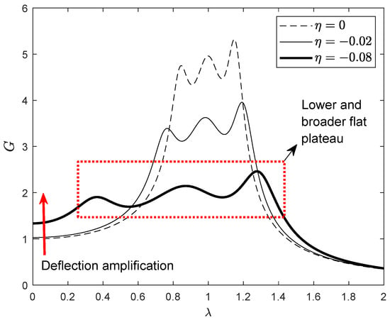
As depicted in Figure 6, the employment of negative stiffness does enhance the overall vibration-control performance, leading to a lower and broader flat plateau near the resonance region. However, it simultaneously deteriorates the vibration behaviour in the extremely low-frequency zone. One may easily obtain the expression of the normalized static amplitude of the primary system by imposing $\lambda =0$ and substituting the optimal values of $\nu$ and $\beta$ into Equation (13), leading to

$$G_{\mathrm{st}}={\displaystyle \frac{\eta +\mu {\alpha }^2}{\eta +\mu (1+\eta ){\alpha }^2}}$$

(30)

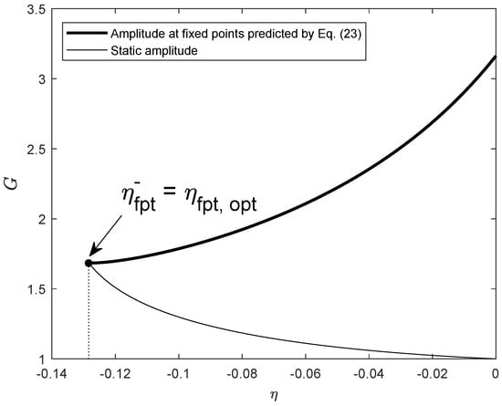
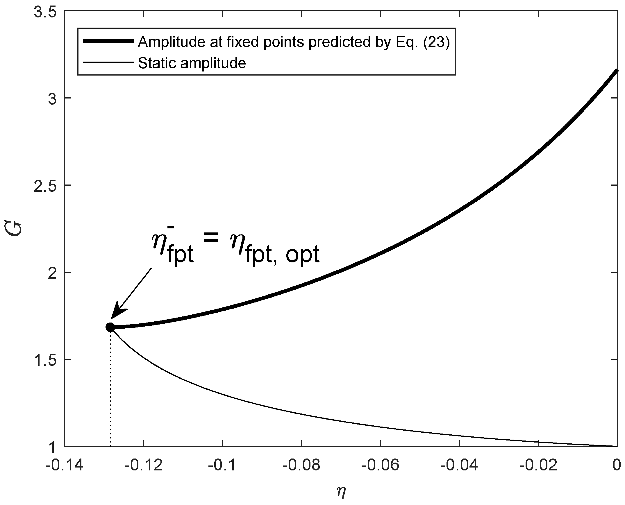
As demonstrated in Figure 7, $G_{\mathrm{st}}$ (indicated by the thin solid line) increases monotonically as the negative stiffness ratio $\eta$ decreases to its lower threshold, which is opposite to that of the normalized vibration amplitude at fixed points (the thick solid line). Therefore, an optimal value of the negative stiffness ratio $\eta$ is herein defined as the one that equates the amplitude at fixed points and static deflection. By imposing $G_{\mathrm{st}}=\sqrt{h_{\mathrm{fpt}}}$, one may easily find that the optimal value of the negative stiffness ratio $\eta$ is exactly the same as its allowable minimum, i.e., ${\eta }_{\mathrm{fpt},\mathrm{opt}}={\eta }_{\mathrm{fpt}}^{-}$, which is also evidenced by Figure 7.

Figure 6. FRFs of the primary system coupled with an NSIDVA optimized by the FPT for the negative stiffness ratio $\eta =0,-0.02,-0.08$.

Figure 7. Evolution of the normalized vibration amplitude at fixed points (thick line) and the normalized static amplitude (thin line) of the primary system with respect to the negative stiffness ratio $\eta$ when optimized by the FPT with a mass ratio $\mu =0.1$.

3.2. Calibration Based on the Stability Maximization Criterion

In this subsection, the parameters of the NSIDVA are calibrated using the stability maximization criterion so as to accelerate the response to transient disturbances. For a classical problem in which an SDOF structure is controlled by an SDOF mechanical absorber, the design objective of optimally shaping the transient response is achieved by coinciding the two pairs of complex conjugate eigenvalues of the coupled system [9]. The structure in question, as sketched out in Figure 1, has three DOFs and six distinct poles, as is evident from its characteristic equation, i.e., the denominator in Equation (12). It has been postulated and theoretically proven in Ref. [13] that for such a coupled system of three DOFs, the transient response of the host structure is optimized when it has three coalesced pairs of conjugate poles. Therefore, one may suppose the optimized eigenvalues have the form of ${\overline{s}}_1={\overline{s}}_3={\overline{s}}_5=-p+j\sqrt{r^2-p^2}$ and ${\overline{s}}_2={\overline{s}}_4={\overline{s}}_6=-p-j\sqrt{r^2-p^2}$, where the positive p and r denote, respectively, the absolute value of the real part and the complex magnitude of all six poles. Thus, the optimized characteristic equation could be recast into the following factorized form and further rearranged as

$$\begin{array}{cc}\hfill f_1\left(\overline{s}\right)& =(\overline{s}-{\overline{s}}_1)·(\overline{s}-{\overline{s}}_2)·(\overline{s}-{\overline{s}}_3)·(\overline{s}-{\overline{s}}_4)·(\overline{s}-{\overline{s}}_5)·(\overline{s}-{\overline{s}}_6)\hfill \\ \hfill & ={\overline{s}}^6+E_5{\overline{s}}^5+E_4{\overline{s}}^4+E_3{\overline{s}}^3+E_2{\overline{s}}^2+E_1\overline{s}+E_0\hfill \end{array}$$

(31)

with the coefficients before terms given by:

$$\begin{array}{cccccc}\hfill E_5& =6p,\hfill & \hfill E_4& =12p^2+3r^2,\hfill & \hfill E_3& =8p^3+12p{r}^2,\hfill \\ \hfill E_2& =12p^2{r}^2+3r^4,\hfill & \hfill E_1& =6p{r}^4,\hfill & \hfill E_0& =r^6.\hfill \end{array}$$

(32)

Meanwhile, the characteristic equation of the concerned system, i.e., the denominator in Equation (12), can be altered into the form of a monic polynomial, i.e.,

$$f_2\left(\overline{s}\right)={\overline{s}}^6+F_5{\overline{s}}^5+F_4{\overline{s}}^4+F_3{\overline{s}}^3+F_2{\overline{s}}^2+F_1\overline{s}+F_0$$

(33)

with its six coefficients defined as:

$$F_k={\displaystyle \frac{D_k}{D_6}},k=0,1,\dots ,5.$$

(34)

Clearly, the optimal scenario occurs when $f_2\left(\overline{s}\right)=f_1\left(\overline{s}\right)$, which is equivalent to:

$$E_k=F_k,k=0,1,\dots ,5.$$

(35)

Up to now, one has six equality conditions (35) associated with the six unknown variables $\nu$, $\alpha$, $\beta$, $\xi$, p and r. Upon further dissection of the expressions of $F_k$, one may find the existence of a linear constraint among $F_0$, $F_1$ and $F_5$ that

$$F_0{F}_5-{\beta }^2{F}_1=0$$

(36)

which is equivalent to $E_0{E}_5-{\beta }^2{E}_1=0$, yielding the formula of the optimal frequency tuning ratio ${\beta }_{\mathrm{smc}}$:

$${\beta }_{\mathrm{smc}}=r$$

(37)

By back substituting Equation (37) into Equation (35) and by solving them simultaneously, the optimal parameters of the NSIDVA can be analytically formulated as a function of the mass ratio $\mu$, negative stiffness ratio $\eta$ and complex magnitude of magnitude r, as follows:

• The natural frequency ratio between the absorber and primary system, $\alpha$, is equal to:

  $${\alpha }_{\mathrm{smc}}=\sqrt{{\displaystyle \frac{\mu r^4-\eta }{\mu (1+\eta )}}}$$

  (38)
• The inertance-to-mass ratio $\nu$ is expressed as:

  $${\nu }_{\mathrm{smc}}={\displaystyle \frac{8\left[\left({\mu }^2+\mu \right)r^4-2\mu \left(1+\eta \right)r^2+\mu +{\eta }^2\right]}{r^2\left(1+\eta \right)}}$$

  (39)
• The mechanical damping ratio $\xi$ is given by:

  $${\xi }_{\mathrm{smc}}={\displaystyle \frac{4\sqrt{3}}{9}}\sqrt{{\displaystyle \frac{\left({\mu }^2+\mu \right)r^4-2\mu \left(1+\eta \right)r^2+\mu +{\eta }^2}{\mu r^4-\eta }}}$$

  (40)
• The absolute value of the real part of all poles, p, is formulated as:

$$p_{\mathrm{smc}}=\sqrt{{\displaystyle \frac{3}{4}}·{\displaystyle \frac{\left({\mu }^2+\mu \right)r^4-2\mu \left(1+\eta \right)r^2+\mu +{\eta }^2}{\mu \left(1+\eta \right)}}}$$

(41)

Finally, the optimal value of r is the root of the following quadratic equation in $r^2$:

$$\mu r^4-\left(1+\eta \right)r^2+1=0$$

(42)

which yields two possible solutions for $r^2$, i.e.,

$$\begin{array}{cccc}\hfill r_1^2& ={\displaystyle \frac{1+\eta -\sqrt{{\left(1+\eta \right)}^2-4\mu }}{2\mu }},\hfill & \hfill r_2^2& ={\displaystyle \frac{1+\eta +\sqrt{{\left(1+\eta \right)}^2-4\mu }}{2\mu }}.\hfill \end{array}$$

(43)

As required by the complex pole assumption, the magnitude of the real part should never be greater than the complex magnitude, namely $p\le r$, imposing an inequality condition on $r^2$:

$$\begin{array}{c}\hfill 3({\mu }^2+\mu )r^4-10\mu \left(1+\eta \right)r^2+3{\eta }^2+3\mu \le 0\end{array}$$

(44)

Therefore, the value of $r^2$ should be bounded by $r^2\in [r_{-}^2,r_{+}^2]$, with the lower and upper thresholds corresponding to:

$$\begin{array}{cc}\hfill r_{-}^2& ={\displaystyle \frac{5\mu \left(1+\eta \right)-\sqrt{\mu \left[\left(16\mu -9\right){\eta }^2+50\mu \eta +\mu \left(16-9\mu \right)\right]}}{3({\mu }^2+\mu )}},\hfill \\ \hfill r_{+}^2& ={\displaystyle \frac{5\mu \left(1+\eta \right)+\sqrt{\mu \left[\left(16\mu -9\right){\eta }^2+50\mu \eta +\mu \left(16-9\mu \right)\right]}}{3({\mu }^2+\mu )}}.\hfill \end{array}$$

(45)

When the negative stiffness is excluded, i.e., $\eta =0$, one may find that $r_{-}^2<r_1^2<r_{+}^2$ and $r_2^2>r_{+}^2$ always hold for $\mu <0.25$, beyond which engineering solutions become impractical. Therefore, the closed-form solution to r is eventually expressed as:

$$r_{\mathrm{smc}}=\sqrt{{\displaystyle \frac{1+\eta -\sqrt{{\left(1+\eta \right)}^2-4\mu }}{2\mu }}}$$

(46)

Similarly, the stability requirement imposes a condition on the allowable value of the negative stiffness ratio $\eta$ that

$$\eta \ge {\eta }_{\mathrm{smc}}^{-}={\displaystyle \frac{9\mu -(6-14\mu )\sqrt{3\mu }}{9-12\mu }}$$

(47)

whose detailed derivation is described in Appendix B.2.

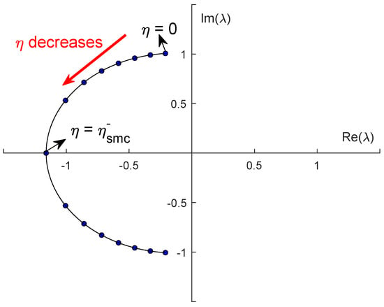
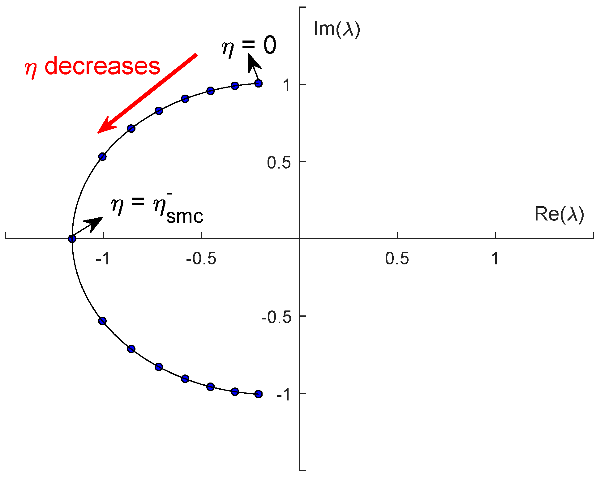
Figure 8 plots the change in complex eigenvalues of the optimized coupled system with respect to the negative stiffness ratio $\eta$. One can infer that as the magnitude of negative stiffness becomes larger, the corresponding complex conjugate eigenvalues move far away from the imaginary axis and get closer to the real axis, representing a better performance in terms of attenuating transient responses. In the extreme case where $\eta ={\eta }_{\mathrm{smc}}^{-}$, the constraint $p\le r$ is satisfied with equality, and all six eigenvalues lose their imaginary parts and become real numbers, indicating that the system reaches a critical state of optimal stability.

Figure 8. Evolution of the root loci of the primary system coupled with an NSIDVA versus the negative stiffness ratio $\eta$ in the SMC-based optimal scenario with a mass ratio $\mu =0.05$.

From a practical standpoint, the negative stiffness ratio $\eta$ can be adjusted by varying the pre-compression of the spring in the rigid link-spring mechanism [23], modifying the geometric parameters of the bistable beam, or employing adjustable electromagnetic negative stiffness mechanisms. It should be emphasized that the value of $\eta$ is bounded by the stability constraint ($\eta \ge {\eta }_{\mathrm{smc}}^{-}$), and the optimal value defined in this paper ($\eta ={\eta }_{\mathrm{smc}}^{-}$) represents the performance limit. In practical design, a margin should be reserved between the employed negative stiffness ratio and its theoretical lower threshold to ensure system robustness.

4. Numerical Simulation and Analyses

In this section, the performance of the proposed NSIDVA is assessed by comparing it with the classical mechanical dampers reported in the literature, namely the non-traditional DVA and the non-traditional IDVA. Both harmonic and transient excitation scenarios will be considered and the corresponding frequency- and time-domain responses generated in order to achieve a better and more comprehensive understanding of the effect of negative stiffness on the overall vibration-control capability. Unless otherwise specified, the mass ratio used for simulation is set as: $\mu =0.05$.

4.1. Frequency-Domain Analyses

It should be noted that the displacement amplification factor $G\left(\lambda \right)=|{\displaystyle \frac{X}{F/k_s}}|$ employed throughout this paper is equivalent to the displacement transmissibility ratio under direct force excitation. The FRFs presented in Figure 9 therefore characterize the frequency-domain transmissibility of the primary system. The extension of the present optimization framework to base excitation scenarios, where the displacement transmissibility ratio $T={\displaystyle \frac{X_{\mathrm{output}}}{X_{\mathrm{input}}}}$ is the standard index, is planned for future work.

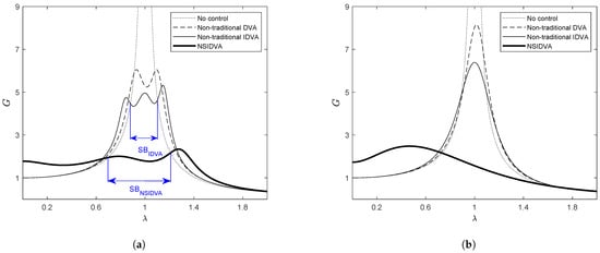
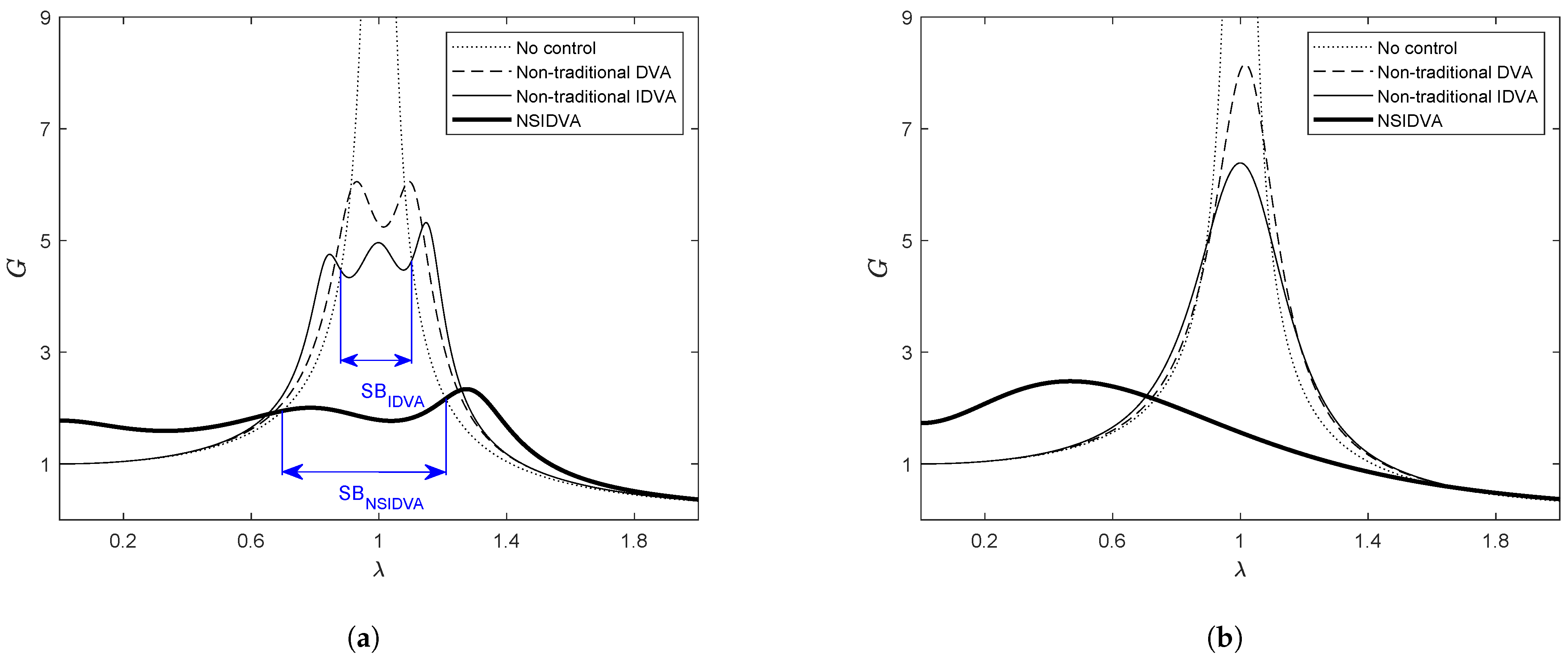
Figure 9. FRFs of primary system controlled by non-traditional DVA (dash line), non-traditional IDVA (thin solid line) or NSIDVA (thick solid line) whose parameters are tuned by: (a) FPT; (b) SMC. Suppression bandwidths normalized by fundamental frequency of primary system are, respectively, ${\mathrm{SB}}_{\mathrm{DVA}}=0.170$, ${\mathrm{SB}}_{\mathrm{IDVA}}=0.223$, ${\mathrm{SB}}_{\mathrm{NSIDVA}}=0.512$.

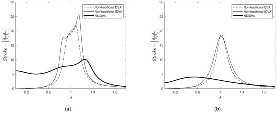
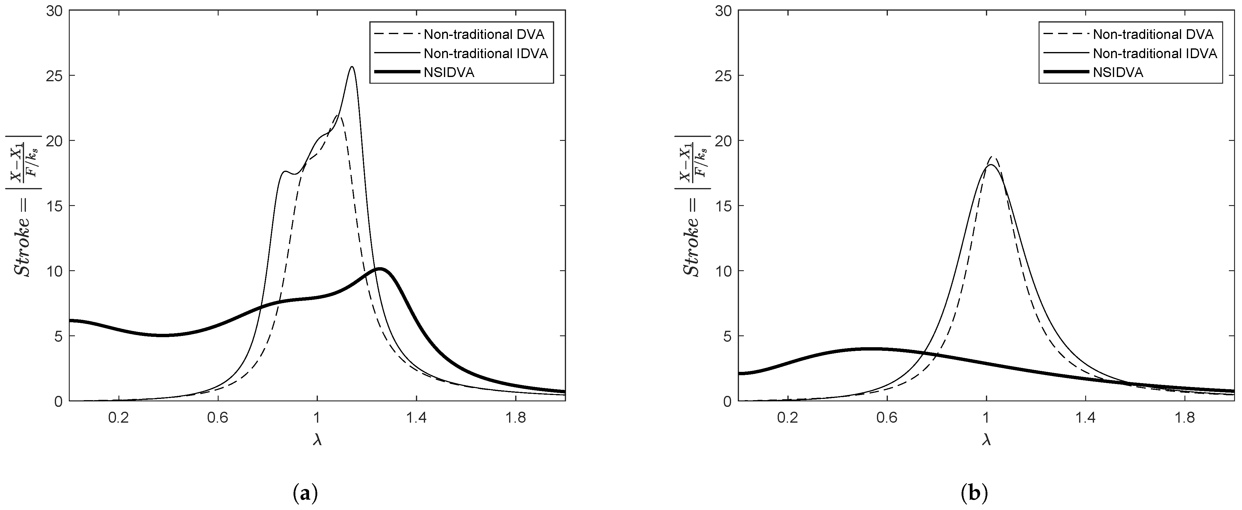
Figure 9 shows the FRFs of the primary system when controlled by the non-traditional DVA (dashed line), the non-traditional IDVA (thin solid line), or the proposed NSIDVA (thick solid line). Figure 9a corresponds to the responses under the FPT-based optimal design, in which the peak amplitudes of the primary system with different types of damper are $6.05$, $5.32$ and $2.34$, respectively, while the suppression bandwidths are $0.170$, $0.223$ and $0.512$, respectively. By comparing the non-traditional IDVA and NSIDVA, the employment of negative stiffness contributes to reducing the peak amplitude by $56\%$ and widening the effective bandwidth of vibration control by $129.6\%$. In general, one can observe that the novel NSIDVA with an optimal negative stiffness ratio exhibits the best control performance in terms of minimizing the peak vibration amplitude and broadening the suppression bandwidth of vibration confinement, while the non-traditional DVA performs the worst. In the case of SMC-based optimal design (Figure 9b), the same phenomenon is also observed; therefore, the previous remark remains valid. Finally, one can conclude from the comparison in Figure 9a,b that the FPT is preferable to the SMC for tuning the parameters of vibration absorbers when the aim is to optimally shape the frequency response of the primary system, i.e., to confine the peak amplitude of steady-state vibration and widen the effective bandwidth of vibration suppression. The advantage of employing negative stiffness resides not only in confining the vibration amplitude of the primary system, but also in controlling the stroke amplitude (i.e., the relative displacement between the primary system and main absorber mass). As shown in Figure 10a, the FPT-based NSIDVA can confine the stroke amplitude under the level of $10.14$, achieving a significant vibration reduction of $53.8\%$ and $60.5\%$ relative to the non-traditional DVA and IDVA, respectively. The improvement in stroke amplitude control with the use of negative stiffness is even more pronounced when the absorber parameters are tuned by the SMC, as shown in Figure 10b, in which the stroke reduction ratio increases to more than $77\%$ with respect to non-traditional DVA and IDVA.

Figure 10. FRFs of relative displacement between primary system and main absorber mass (termed as stroke amplitude) when controlled by non-traditional DVA (dash line), non-traditional IDVA (thin solid line) or NSIDVA (thick solid line), whose parameters are tuned by: (a) FPT; (b) SMC.

4.2. Time-Domain Analyses

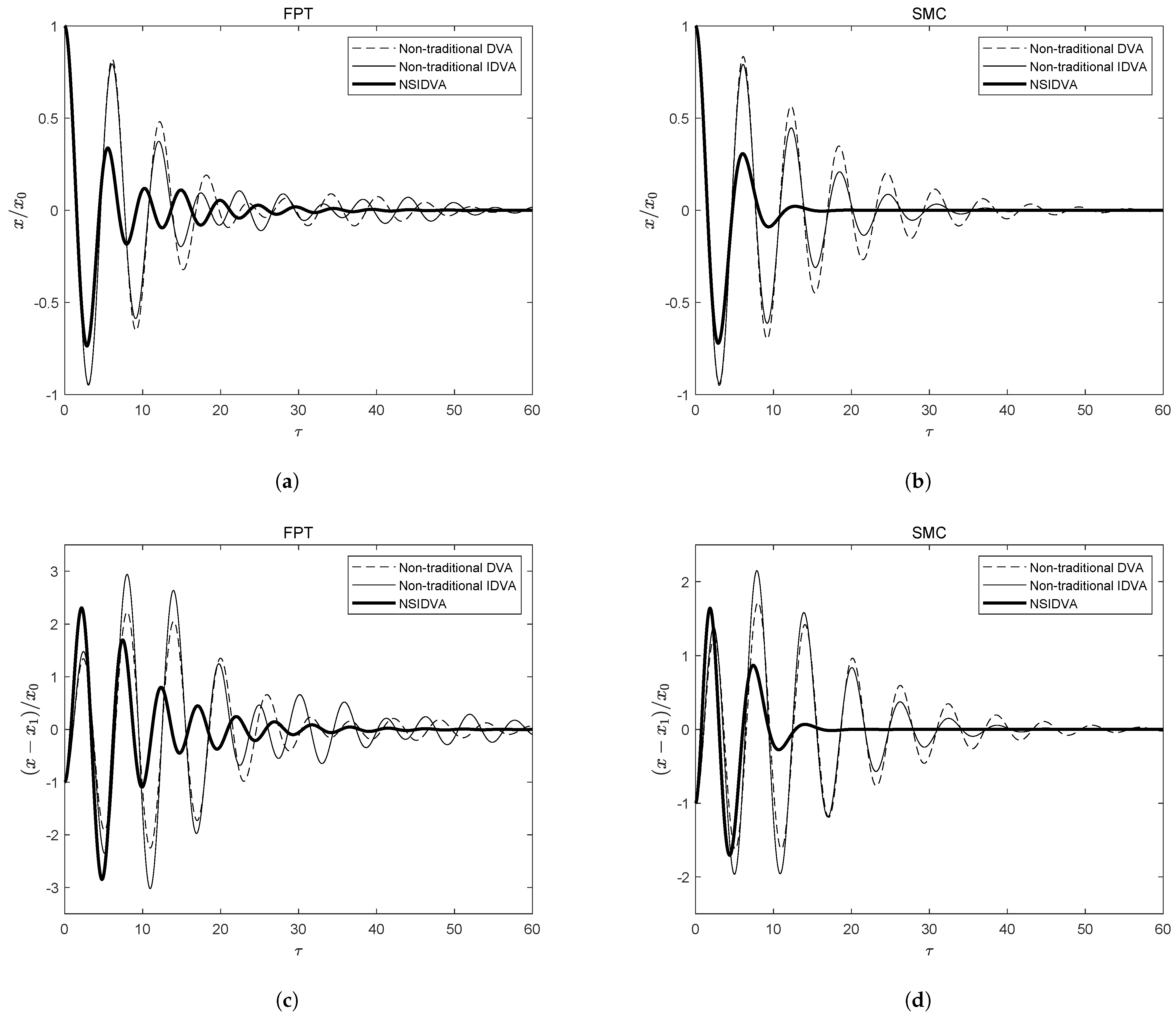
In this subsection, the performance of the different absorbers in controlling transient vibration is investigated. To this end, the temporal responses of the different coupled systems are generated by directly solving their dimensionless equations of motion via the fourth-order Runge–Kutta integration method implemented in Matlab R2023a. The negative stiffness ratio of the NSIDVA is set to $-0.08$, and the time span used for simulation is 60 periods with a time step fixed at $d\tau ={10}^{-4}$. Moreover, the transient vibration is engendered by releasing the mass of the primary system, $m_s$, from a given position while keeping the other parts at rest (i.e., zero displacement and velocity). In this study, the initial displacement of the primary system is set to $x_0=0.1m$.

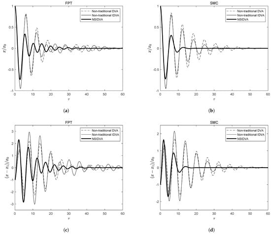
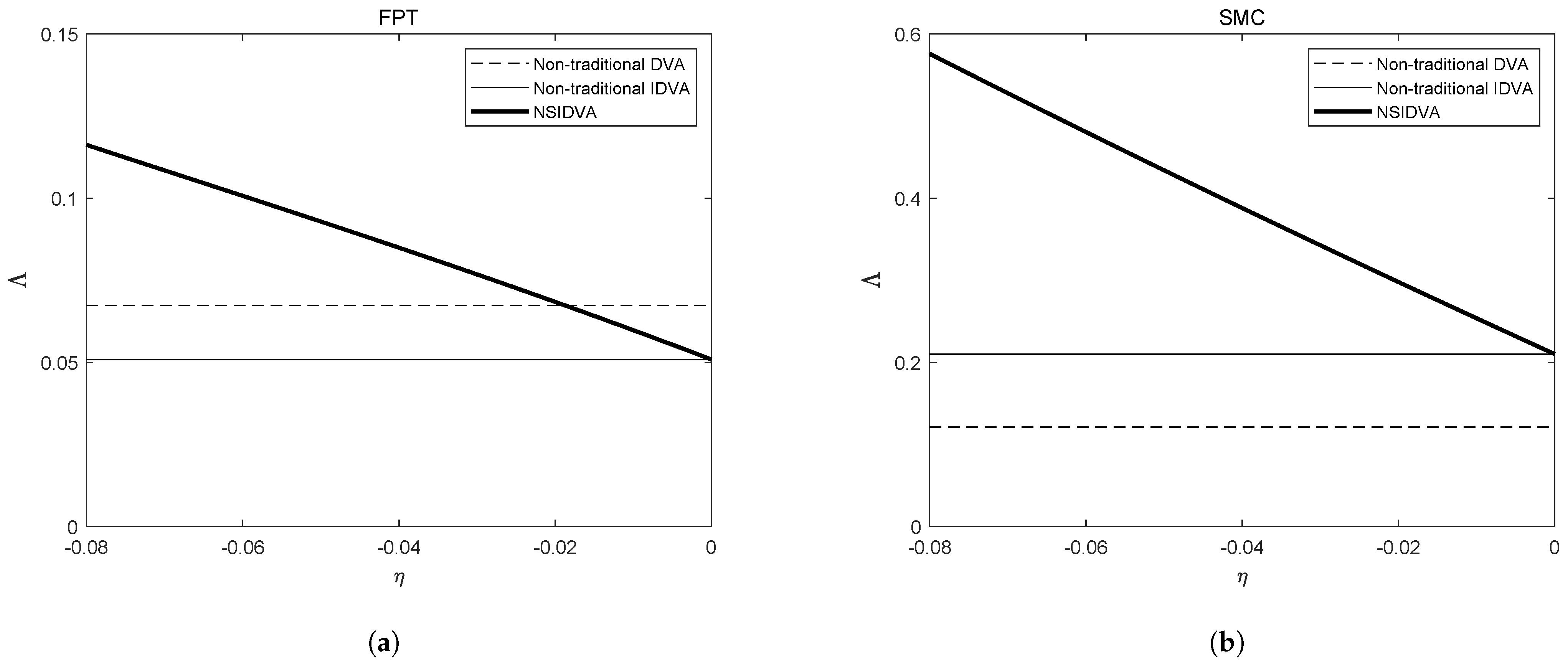
Figure 11 depicts the normalized transient responses of the primary system (Figure 11a,b) and stroke vibration (Figure 11c,d). First, a general conclusion can be drawn by inspecting these figures: the NSIDVA outperforms its two counterparts significantly in attenuating both the transient oscillation of the primary system and the stroke vibration. Secondly, the SMC-based NSIDVA can decay the transient vibration to zero in less than 20 periods, whereas that tuned by the FPT requires more than 50 periods to achieve this. Thus, the SMC is preferable to the FPT when the transient vibration is to be attenuated in the shortest possible time. Finally, an interesting phenomenon is observed: when tuned by the FPT, the non-traditional IDVA attenuates the transient vibrations slightly more slowly than the non-traditional DVA, whereas the opposite holds when it is tuned by the SMC. This could be quantitatively explained by the performance index $\mathsf{\Lambda }$, defined as the minimum absolute value of the real parts of all eigenvalues, namely:

$$\mathsf{\Lambda }=\underset{i}{\min }\left\{\left|\mathrm{Re}\right({\lambda }_i\left)\right|\right\},i=1,2,\dots 6.$$

(48)

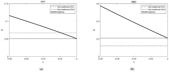
Also termed the degree of stability, the performance index $\mathsf{\Lambda }$ quantifies the overall decay rate of transient oscillation experienced by the coupled system. Figure 12 plots the evolution of $\mathsf{\Lambda }$ against the negative stiffness ratio $\eta$. The performance indices of the non-traditional DVA and IDVA when tuned by the FPT are $0.067$ and $0.051$, and they further increase to $0.121$ and $0.210$, respectively, when calibrated by the SMC, which fully explains this seemingly contradictory behaviour. Furthermore, the performance index of the NSIDVA increases monotonically with the magnitude of the negative stiffness ratio $\eta$, clearly indicating that the use of negative stiffness contributes to accelerating the decay rate of transient vibration in addition to improving the vibration-control performance in the steady state.

Figure 11. Temporal responses of normalized displacement of primary system (a,b) and normalized stroke vibration (c,d). Initial displacement of primary system is set as $x_0=0.1$, negative stiffness ratio $\eta =-0.08$ and other parameters are tuned by: (a,c) FPT; (b,d) SMC.

Figure 12. Evolution of performance index $\mathsf{\Lambda }$ against the negative stiffness ratio $\eta$ when tuned by: (a) the FPT; (b) the SMC.

5. Conclusions

In this work, a novel model of the non-traditional IDVA with negative stiffness is proposed, and its optimal design determined according to two widely used optimization strategies, namely the FPT and the SMC. The analytical expressions of the tuning parameters are derived and formulated in terms of the mass ratio $\mu$ and negative stiffness ratio $\eta$, and a thorough stability analysis is conducted, yielding the allowable limit on the magnitude of negative stiffness.

The merits of the proposed NSIDVA are demonstrated by comparing it with two existing dampers, the non-traditional DVA and IDVA. The numerical results, obtained under a mass ratio of $\mu =0.05$ and a negative stiffness ratio of $\eta =-0.08$, show that, compared with the non-traditional IDVA, the NSIDVA with the optimal negative stiffness ratio can further reduce the peak amplitude by $56\%$ and widen the effective bandwidth of vibration suppression by $129.6\%$, which outperforms the non-traditional DVA by a much larger margin. It should be noted that these quantitative improvements are specific to the aforementioned parameter settings, and the actual degree of improvement depends on the mass ratio and the magnitude of negative stiffness employed. Nevertheless, as evidenced by Figure 12, the performance index $\mathsf{\Lambda }$ increases monotonically with the magnitude of the negative stiffness ratio, suggesting a consistent trend of improvement across the allowable parameter range. The advantages of employing negative stiffness in the mechanical absorber lie not only in confining the steady-state vibration of the primary system and the stroke vibration more efficiently, but also in the fact that it can increase the system damping level, thereby accelerating the decay of transient vibration.

This work also establishes complete electromechanical analogies between mechanical damping devices (including the classical absorbers reported in the literature and the newly proposed NSIDVA) and piezoelectric shunt dampers. Based on the proposed electromechanical analogies, mechanical absorbers can be fully synthesized by their equivalent piezoelectric shunt dampers, facilitating their practical application in scenarios subject to physical constraints, such as space and weight.

This work conducted optimization only under direct force excitation; thus, further research could be devoted to the optimal design under base excitation with an objective other than the displacement of the primary system.

Appendix B.1. Tuning According to the Extended Fixed-Points Technique

• Non-negative constraint on design parameters.
  • Optimal frequency tuning ratio ${\alpha }_{\mathrm{fpt}}$. To have a real and positive value for $\alpha$, its governing Equation (18) should have a non-negative discriminant, namely $\mathsf{\Delta }={\mu }^2·{\mathsf{\Delta }}_1={\mu }^2\left[{\mu }^2{(1+\eta )}^2-4\mu {\eta }^2\right]\ge 0$, yielding the first lower bound on $\eta$:

    $$\eta \ge {\eta }_{\mathrm{fpt},1}^{-}={\displaystyle \frac{\mu -2\sqrt{\mu }}{4-\mu }}$$

    (A7)
  • Optimal inertance-to-mass ratio ${\nu }_{\mathrm{fpt}}$. The non-negativity of ${\nu }_{\mathrm{fpt}}$ leads to an inequality condition, as follows:

    $$m_0·\sqrt{{\mathsf{\Delta }}_1}+m_1\ge 0$$

    (A8)

    with $m_0$ and $m_1$ given by:

    $$\begin{array}{cc}\hfill m_0& =\left(-{\mu }^4+9{\mu }^3-27{\mu }^2+30\mu -9\right){\eta }^3+\left(-3{\mu }^4+17{\mu }^3-25{\mu }^2+6\mu +1\right){\eta }^2\hfill \\ & +\left(-3{\mu }^4+9{\mu }^3-4{\mu }^2\right)\eta -{\mu }^4+{\mu }^3\hfill \\ \hfill m_1& =\left(-{\mu }^5+11{\mu }^4-43{\mu }^3+70{\mu }^2-41\mu +4\right){\eta }^4+\left(-4{\mu }^5+30{\mu }^4-68{\mu }^3+44{\mu }^2\right){\eta }^3\hfill \\ & +\left(-6{\mu }^5+28{\mu }^4-31{\mu }^3+6{\mu }^2-\mu \right){\eta }^2+\left(-4{\mu }^5+10{\mu }^4-4{\mu }^3\right)\eta -{\mu }^5+{\mu }^4\hfill \end{array}$$

    (A9)
    With the help of Maple, it is clear that for $\mu \in [0,0.25]$ and $\eta \in [-1,0]$, which cover the most practical engineering applications, $m_0\ge 0$ always holds while $m_1\le 0$ is mostly encountered, except for regions extremely close to $\eta =-1$. Therefore, the inequality (A8) could be recast into the condition $m_0^2·{\mathsf{\Delta }}_1-m_1^2\ge 0$, which results in a quadratic polynomial in $\eta$:

    $$(4-\mu ){\eta }^2-2\mu \eta +{\mu }^2-\mu \le 0$$

    (A10)
    Thus, a second lower limit of the negative stiffness ratio is obtained:

    $$\eta \ge {\eta }_{\mathrm{fpt},2}^{-}={\displaystyle \frac{\mu -(2-\mu )\sqrt{\mu }}{4-\mu }}$$

    (A11)
  Meanwhile, the non-negativity of ${\beta }_{\mathrm{fpt}}$, ${\xi }_{\mathrm{fpt}}$ and $h_{\mathrm{fpt}}$ is automatically secured as the above two constraints are satisfied.
• The stability requirement. As evident from Equation (A6), $d_0$, $d_1$ and $d_2$ should be no less than zero given that all design parameters are non-negative. Other constraints on negative stiffness are then specified so as to render $d_3$, $d_4$, $d_5$ and $d_6$ non-negative.
  • $d_3$. By substituting the expression of ${\alpha }_{\mathrm{fpt}}$, $d_3={\nu }^2{\beta }^2\left(\sqrt{{\mathsf{\Delta }}_1}+\mu (1+\eta )\right)/2(\mu +\nu )\ge 0$ always holds.
  • $d_4$ and $d_5$. Their non-negativity imposes the same inequality $m_2·m_3\ge 0$, with the two polynomials expressed as:

    $$\begin{array}{cc}\hfill m_2& =(4-\mu ){\eta }^2-2\mu \eta +{\mu }^2-\mu \hfill \\ \hfill m_3& =\left(-{\mu }^2+4\mu -4\right){\eta }^4+\left(-6{\mu }^2+4\mu \right){\eta }^2+4\eta {\mu }^3-{\mu }^4-{\mu }^2\hfill \end{array}$$

    (A12)

    in which $m_3\le 0$ is always met for $\mu \in [0,0.25]$ and $\eta \in [-1,0]$. Thus, $m_2\le 0$ should be satisfied, which is exactly the condition in (A10).
  • $d_6$. $d_6\ge 0$ is rewritten as $m_4·\sqrt{{\mathsf{\Delta }}_1}+m_5\ge 0$ with $m_4=1+\eta$ and $m_5=\mu {(1+\eta )}^2-2{\eta }^2$. Given $m_4\ge 0$, there exist two possible cases derived from this inequality, as discussed one by one below. Case I: $m_5\le 0$ and $m_4·\sqrt{{\mathsf{\Delta }}_1}\ge -m_5\ge 0$. However, one may find immediately that $m_4^2·{\mathsf{\Delta }}_1-m_5^2=-4{\eta }^4\le 0$. Thus, this case is unrealistic, and $m_5$ should never be inferior to zero. Case II: $m_5\ge 0$. In this scenario, the concerned inequality condition is naturally satisfied while $m_5\ge 0$ engenders a third lower threshold for the negative stiffness ratio:

    $$\eta \ge {\eta }_{\mathrm{fpt},3}^{-}={\displaystyle \frac{\mu -\sqrt{2\mu }}{2-\mu }}$$

    (A13)

In conclusion, an acceptable value of the negative stiffness ratio $\eta$ should be located within the allowable interval, i.e., $[{\eta }_{\mathrm{fpt}}^{-},0]$, whose lower limit is defined as:

$${\eta }_{\mathrm{fpt}}^{-}=\max \left\{{\eta }_{\mathrm{fpt},1}^{-},{\eta }_{\mathrm{fpt},2}^{-},{\eta }_{\mathrm{fpt},3}^{-}\right\}={\displaystyle \frac{\mu -(2-\mu )\sqrt{\mu }}{4-\mu }}$$

(A14)

Appendix B.2. Tuning According to the Stability Maximization Criterion

In addition to the two constraints previously mentioned, there exists an additional constraint on the negative stiffness arising from the complex pole assumption adopted in this pole-based optimization, which stipulates that the magnitude of the real part of any pole should never exceed its complex magnitude.

• Non-negative constraint on design parameters.
  • Optimal complex magnitude $r_{\mathrm{smc}}$ (also the frequency tuning ratio ${\beta }_{\mathrm{smc}}$). To have a real and positive value for r, a non-negative discriminant should be preserved for its governing Equation (42). In this context, ${\mathsf{\Delta }}_2={(1+\eta )}^2-4\mu \ge 0$ should be satisfied and one can obtain a first lower bound on $\eta$:

    $$\eta \ge {\eta }_{\mathrm{smc},1}^{-}=2\sqrt{\mu }-1$$

    (A15)
  • Optimal frequency tuning ratio ${\alpha }_{\mathrm{smc}}$. Its non-negativity is assured if $n_0·\sqrt{{\mathsf{\Delta }}_2}+n_1\le 0$ with $n_0=1$ and $n_1=2\mu -\eta -1$. It is equivalent to have $n_1\le 0$ and $n_1^2-n_0^2·{\mathsf{\Delta }}_2=4\mu (\mu -\eta )\ge 0$, in which the latter condition is always satisfied for any negative $\eta$, while the former one results in:

    $$\eta \ge {\eta }_{\mathrm{smc},2}^{-}=2\mu -1$$

    (A16)
  • Optimal inertance-to-mass ratio ${\nu }_{\mathrm{smc}}$ (also the mechanical damping ratio ${\xi }_{\mathrm{smc}}$ and magnitude of the real part of pole $p_{\mathrm{smc}}$). Their non-negativity imposes identically that $n_2·\sqrt{{\mathsf{\Delta }}_2}+n_3\le 0$ with $n_2=1-\mu$ and $n_3=3\mu -1-(1+\mu )\eta$. Similar to the previous case, the equivalent conditions are $n_3\le 0$ and $n_3^2-n_2^2·{\mathsf{\Delta }}_2=4\mu {(\mu -\eta )}^2\ge 0$, suggesting a third lower threshold of $\eta$:

    $$\eta \ge {\eta }_{\mathrm{smc},3}^{-}={\displaystyle \frac{3\mu -1}{\mu +1}}$$

    (A17)
• Requirement of complex pole assumption (i.e., $p_{\mathrm{smc}}\le r_{\mathrm{smc}}$). This requirement equivalently imposes that $n_4·\sqrt{{\mathsf{\Delta }}_2}+n_5\le 0$ with $n_4=7\mu -3$ and $n_5=(3-\mu )\eta +3-13\mu$. For $\mu \in [0,0.25]$, $n_4<0$. Again, two possible scenarios may exist for this condition. First, $n_5$ should be non-positive and the current inequality is fulfilled naturally. However, $n_5\le 0$ imposes $\eta \le (13\mu -3)/(3-\mu )$, which contrasts sharply with cases previously discussed and should thus be neglected. Hence, one should have $n_5\ge 0$ and $n_4^2·{\mathsf{\Delta }}_2-n_5^2=(12\mu -9){\eta }^2+18\mu \eta +12\mu -49{\mu }^2\ge 0$, each of which imposes a constraint on the negative stiffness ratio:

  $$\begin{array}{cccc}\hfill \eta & \ge {\eta }_{\mathrm{smc},4}^{-}={\displaystyle \frac{13\mu -3}{3-\mu }},\hfill & \hfill \eta & \ge {\eta }_{\mathrm{smc},5}^{-}={\displaystyle \frac{9\mu -(6-14\mu )\sqrt{3\mu }}{9-12\mu }}.\hfill \end{array}$$

  (A18)
• The stability requirement. In this case, only $d_3$ should be carefully considered while the other elements remain non-negative. The non-negativity of $d_3$ leads to $n_6·\sqrt{{\mathsf{\Delta }}_2}+n_7\le 0$ with $n_6=1$ and $n_7=2\mu -1-(2\mu +1)\eta$. Clearly, it is equivalent to have $n_7\le 0$ and $n_7^2-n_6^2·{\mathsf{\Delta }}_2=4\mu (\mu {\eta }^2+{\eta }^2+\mu -2\mu \eta )\ge 0$. Clearly, the latter condition is fulfilled for any negative $\eta$, while the former yields a sixth lower limit on $\eta$:

$$\eta \ge {\eta }_{\mathrm{smc},6}^{-}={\displaystyle \frac{2\mu -1}{2\mu +1}}$$

(A19)

Finally, the lower threshold of the negative stiffness ratio when calibrated by the stability maximization criterion, ${\eta }_{\mathrm{smc}}^{-}$, should be chosen as:

$${\eta }_{\mathrm{smc}}^{-}=\max \left\{{\eta }_{\mathrm{smc},1}^{-},{\eta }_{\mathrm{smc},2}^{-},{\eta }_{\mathrm{smc},3}^{-},{\eta }_{\mathrm{smc},4}^{-},{\eta }_{\mathrm{smc},5}^{-},{\eta }_{\mathrm{smc},6}^{-}\right\}={\displaystyle \frac{9\mu -(6-14\mu )\sqrt{3\mu }}{9-12\mu }}$$

(A20)

References

- Yu, Y.; Wang, C.; Wang, W.; Lu, K.; Chen, Z.; Zhao, D.; Ju, B.F.; Zhou, S. Determination of elastic constants in unidirectional CFRP laminates using neural networks and laser ultrasonic bulk waves. Compos. Part A Appl. Sci. Manuf. 2026, 10, 109827. [Google Scholar] [CrossRef] [Scilit]
- Wu, X.; Dong, J.; Bao, W.; Zou, B.; Wang, L.; Wang, H. Augmented intelligence of things for emergency vehicle secure trajectory prediction and task offloading. IEEE Internet Things J. 2024, 11, 36030–36043. [Google Scholar] [CrossRef] [Scilit]
- Ormondroyd, J.; Hartog, J. The theory of dynamic vibration absorber. J. Appl. Mech. 1928, 50, 9–22. [Google Scholar]
- Zhu, S.; Yang, J.; Yan, H.; Zhang, L.; Cai, C. Low-frequency vibration control of floating slab tracks using dynamic vibration absorbers. Veh. Syst. Dyn. 2015, 53, 1296–1314. [Google Scholar] [CrossRef] [Scilit]
- Shen, Y.; Chen, L.; Yang, X.; Shi, D.; Yang, J. Improved design of dynamic vibration absorber by using the inerter and its application in vehicle suspension. J. Sound Vib. 2016, 361, 148–158. [Google Scholar] [CrossRef] [Scilit]
- Liu, Y.; Wang, X.; Xue, Y.; Deng, E.; Wang, Y.; Song, C.; Feng, Q. Dynamic analysis of quasi-zero stiffness vibration isolation system coupled with frequency adjustable dynamic vibration absorber. Arch. Appl. Mech. 2022, 92, 3631–3647. [Google Scholar] [CrossRef] [Scilit]
- Zhou, S.; Jean-Mistral, C.; Chesne, S. Influence of inerters on the vibration control effect of series double tuned mass dampers: Two layouts and analytical study. Struct. Control Health Monit. 2019, 26, e2414. [Google Scholar] [CrossRef] [Scilit]
- Ren, M.Z. A variant design of the dynamic vibration absorber. J. Sound Vib. 2001, 245, 762–770. [Google Scholar] [CrossRef] [Scilit]
- Zhou, S.; Jean-Mistral, C.; Chesné, S. Closed-form solutions to optimal parameters of dynamic vibration absorbers with negative stiffness under harmonic and transient excitation. Int. J. Mech. Sci. 2019, 157–158, 528–541. [Google Scholar] [CrossRef] [Scilit]
- Hu, Y.; Chen, M.Z.Q. Performance evaluation for inerter-based dynamic vibration absorbers. Int. J. Mech. Sci. 2015, 99, 297–307. [Google Scholar] [CrossRef] [Scilit]
- Smith, M.C. Synthesis of mechanical networks: The inerter. IEEE Trans. Autom. Control 2002, 47, 1648–1662. [Google Scholar] [CrossRef] [Scilit]
- Barredo, E.; Blanco, A.; Colín, J.; Penagos, V.M.; Abúndez, A.; Vela, L.G.; Meza, V.; Cruz, R.H.; Mayén, J. Closed-form solutions for the optimal design of inerter-based dynamic vibration absorbers. Int. J. Mech. Sci. 2018, 144, 41–53. [Google Scholar] [CrossRef] [Scilit]
- Zhou, S.; Jean-Mistral, C.; Chesné, S. Optimal design of an inerter-based dynamic vibration absorber connected to ground. J. Vib. Acoust. 2019, 141, 051017. [Google Scholar] [CrossRef] [Scilit]
- Barredo, E.; Larios, J.M.; Colín, J.; Mayén, J.; Flores-Hernández, A.; Arias-Montiel, M. A novel high-performance passive non-traditional inerter-based dynamic vibration absorber. J. Sound Vib. 2020, 485, 115583. [Google Scholar] [CrossRef] [Scilit]
- Kendo-Nouja, B.; Baduidana, M.; Kenfack-Jiotsa, A.; Nzengwa, R. Vibration reduction of primary structure using optimum grounded inerter-based dynamic vibration absorber. Arch. Appl. Mech. 2024, 94, 137–156. [Google Scholar] [CrossRef] [Scilit]
- Dogan, H.; Sims, N.D.; Wagg, D.J. Design, testing and analysis of a pivoted-bar inerter device used as a vibration absorber. Mech. Syst. Signal Process. 2022, 171, 108893. [Google Scholar] [CrossRef] [Scilit]
- Dogan, H.; Sims, N.D.; Wagg, D.J. Implementation of inerter-based dynamic vibration absorber for chatter suppression. J. Manuf. Sci. Eng. 2023, 145, 084502. [Google Scholar] [CrossRef] [Scilit]
- Dogan, H.; Ozsoy, M.; Ozturk, E.; Wagg, D.J.; Sims, N.D. Analysis of virtual inerter-based passive absorber for active chatter control. J. Sound Vib. 2024, 578, 118359. [Google Scholar] [CrossRef] [Scilit]
- Wang, M.; Du, X.L.; Sun, F.F.; Nagarajaiah, S.; Li, Y.W. Fragility analysis and inelastic seismic performance of steel braced-core-tube frame outrigger tall buildings with passive adaptive negative stiffness damped outrigger. J. Build. Eng. 2022, 52, 104428. [Google Scholar] [CrossRef] [Scilit]
- Chong, X.; Wu, Z.; Li, F. Vibration isolation properties of the nonlinear X-combined structure with a high-static and low-dynamic stiffness: Theory and experiment. Mech. Syst. Signal Process. 2022, 179, 109352. [Google Scholar] [CrossRef] [Scilit]
- Zhang, Y.; Liu, Q.; Lei, Y.; Cao, J.; Liao, W.H. Halbach high negative stiffness isolator: Modeling and experiments. Mech. Syst. Signal Process. 2023, 188, 110014. [Google Scholar] [CrossRef] [Scilit]
- Chen, L.; Liu, Z.; Zou, Y.; Wang, M.; Nagarajaiah, S.; Sun, F.; Sun, L. Practical negative stiffness device with viscoelastic damper in parallel or series configuration for cable damping improvement. J. Sound Vib. 2023, 560, 117757. [Google Scholar] [CrossRef] [Scilit]
- Acar, M.; Yilmaz, C. Design of an adaptive–passive dynamic vibration absorber composed of a string–mass system equipped with negative stiffness tension adjusting mechanism. J. Sound Vib. 2013, 332, 231–245. [Google Scholar] [CrossRef] [Scilit]
- Shen, Y.; Peng, H.; Li, X.; Yang, S. Analytically optimal parameters of dynamic vibration absorber with negative stiffness. Mech. Syst. Signal Process. 2017, 85, 193–203. [Google Scholar] [CrossRef] [Scilit]
- Wang, X.; He, T.; Shen, Y.; Shan, Y.; Liu, X. Parameters optimization and performance evaluation for the novel inerter-based dynamic vibration absorbers with negative stiffness. J. Sound Vib. 2019, 463, 114941. [Google Scholar] [CrossRef] [Scilit]
- Gao, H.; Wang, Z.; Jia, J.; Cheng, Z. The negative stiffness electromagnetic tuned inerter damper for damping enhancement of stay cables. Eng. Struct. 2023, 292, 116542. [Google Scholar] [CrossRef] [Scilit]
- Zhou, S.; Bao, B. A lever-enhanced tuned inerter damper for controlling vibrations due to rotary unbalance and bounded parametric uncertainty: Classic and robust equal-peak optimization. J. Sound Vib. 2025, 596, 118777. [Google Scholar] [CrossRef] [Scilit]
- Wang, Z.H.; Cheng, Z.P.; Yin, G.Z.; Shen, W. A magnetic negative stiffness eddy-current inertial mass damper for cable vibration mitigation. Mech. Syst. Signal Process. 2023, 188, 110013. [Google Scholar] [CrossRef] [Scilit]
- Shi, X.; Guan, X.; Shen, W.; Xing, L. A control strategy using negative stiffness and semi-active viscous damping for fully tracking active control force for bridge cables: Principles and simulations. Struct. Control Health Monit. 2022, 29, e2989. [Google Scholar] [CrossRef] [Scilit]
- Zhao, Z.; Chen, Q.; Hu, X.; Zhang, R. Enhanced energy dissipation benefit of negative stiffness amplifying dampers. Int. J. Mech. Sci. 2023, 240, 107934. [Google Scholar] [CrossRef] [Scilit]
- Xiao, L.; Bursi, O.S.; Wang, M.; Nagarajaiah, S.; Sun, F.; Du, X.L. Metamaterial beams with negative stiffness absorbers and rotation: Band-gap behavior and band-gap merging. Eng. Struct. 2023, 280, 115702. [Google Scholar] [CrossRef] [Scilit]
- Høgsberg, J. Vibration control by piezoelectric proof-mass absorber with resistive-inductive shunt. Mech. Adv. Mater. Struct. 2021, 28, 141–153. [Google Scholar] [CrossRef] [Scilit]
- Yamada, K.; Asami, T. Passive vibration suppression using 2-degree-of-freedom vibration absorber consisting of a beam and piezoelectric elements. J. Sound Vib. 2022, 532, 116997. [Google Scholar] [CrossRef] [Scilit]
- Zhou, S.; Bao, B. Investigation on high-order resonant electromagnetic shunt dampers for vibration control: Methodology and optimum tuning. Struct. Control Health Monit. 2022, 29, e3094. [Google Scholar] [CrossRef] [Scilit]
- Ding, B.; Li, X.; Chen, S.C.; Li, Y. Modular quasi-zero-stiffness isolator based on compliant constant-force mechanisms for low-frequency vibration isolation. J. Vib. Control 2024, 30, 3006–3020. [Google Scholar] [CrossRef] [Scilit]
- Kim, S.M.; Wang, S.; Brennan, M.J. Dynamic analysis and optimal design of a passive and an active piezo-electrical dynamic vibration absorber. J. Sound Vib. 2011, 330, 603–614. [Google Scholar] [CrossRef] [Scilit]
- Gripp, J.; Rade, D. Vibration and noise control using shunted piezoelectric transducers: A review. Mech. Syst. Signal Process. 2018, 112, 359–383. [Google Scholar] [CrossRef] [Scilit]
- Hu, Y.; Chen, M.Z.; Shu, Z.; Huang, L. Analysis and optimisation for inerter-based isolators via fixed-point theory and algebraic solution. J. Sound Vib. 2015, 346, 17–36. [Google Scholar] [CrossRef] [Scilit]
- Marian, L.; Giaralis, A. Optimal design of a novel tuned mass-damper–inerter (TMDI) passive vibration control configuration for stochastically support-excited structural systems. Probabilistic Eng. Mech. 2014, 38, 156–164. [Google Scholar] [CrossRef] [Scilit]
Disclaimer/Publisher’s Note: The statements, opinions and data contained in all publications are solely those of the individual author(s) and contributor(s) and not of MDPI and/or the editor(s). MDPI and/or the editor(s) disclaim responsibility for any injury to people or property resulting from any ideas, methods, instructions or products referred to in the content. |
© 2026 by the authors. Licensee MDPI, Basel, Switzerland. This article is an open access article distributed under the terms and conditions of the Creative Commons Attribution (CC BY) license.