Modelling Study for Turbulent Combustion of Carbon Deposits Collected from Coke-Oven Walls

Abstract

Accumulation of carbon deposits on coke-oven walls is an inherent challenge. The air injection technique for removing them is becoming widely adopted in coke-oven operations. A physical model that simulates the turbulent reacting flow of this carbon-deposit removal process is necessary to serve as a numerical analysis tool. Due to a lack of available measurement data for the rate of carbon deposit removal in coke ovens, benchmark data from thermogravimetric experiments were used to validate a developed turbulent combustion model. This study compares the simulation performance of one-film and two-film models for the reaction of carbon deposits and air, as well as turbulence–reaction interactions, these being the eddy dissipation model and a beta-shape probability density function (PDF) method. The physical model using the SST k-ω turbulence model, the two-film model for carbon–air reactions, and a beta-shape PDF method can account for turbulence–reaction interactions and simulate turbulent burning carbon-deposit tests in TG experiments. This model can simulate carbon deposit removal in coke ovens through air injection.

1. Introduction

1.1. Background and Industrial Relevance

Coke plays an indispensable dual role in blast furnaces for ironmaking, serving as both the primary fuel and a crucial reducing agent. The production of metallurgical coke involves pyrolyzing coal blends and then carbonizing them at high temperatures in coke-oven chambers. During this process, volatile matter composed predominantly of hydrocarbons is released from the charged coal. Thermal decomposition of these volatiles, in the high-temperature free space above the coal bed, can produce undesirable carbon deposits on the furnace refractory walls or in the gas offtake system. A second mechanism also contributes to this buildup. Fine coal particles entrained during charging are deposited on the furnace walls and subsequently carbonized into compact layers. Nakagawa et al. [1] showed that fine coal particles entrained under coal moisture control (CMC) operation increased the deposit mass by 45 to 75 percent in laboratory tests. This finding highlights the role that entrained fine coal particles play in deposit formation under a specific operational process.

These deposits form a complex composite material consisting of two distinct carbonaceous phases. One is a dense, graphitic pyrolytic carbon formed from cracking of the coke-oven gas. The other is a more porous char resulting from devolatilization of the entrained fine particles. Their progressive accumulation, cycle after cycle, creates significant operational challenges for the coke oven. These include clogging of the pusher ram’s path, which increases the required pushing force and impedes discharge of the finished coke, and choking of the ascension pipes, which hinders outflow of the coke-oven gas. Research by Sugiura et al. [2] quantitatively linked carbon deposition to increased pushing loads. This elevates the risk of mechanical damage to the pusher machine and the refractory lining. It also causes frequent production downtime to clean deposited carbon, which reduces coke production. Progressive accumulation of carbon deposits reduces the heat transfer coefficients on the walls between each coke-oven chamber and its two neighboring combustion chambers. It then increases fuel consumption in the two neighboring combustion chambers to maintain the same carbonization process.

Identifying an efficient removal strategy for these carbon deposits, rather than relying on traditional manual removal during maintenance downtime, is essential. This strategy helps maintain optimal coke-oven performance, ensures operational safety, and prolongs the equipment’s lifespan. In practice, deposit removal occurs during the inter-cycle period, when the oven chamber is empty, by introducing an oxygen-containing gas such as air. This is done through natural convection, by opening the charging holes and oven doors, or through forced convection, using a specialized air-blowing lance. Importantly, these methods’ ability to remove deposits within an operating coke oven has been the subject of little experimental or numerical research to date. During carbonization, operating conditions vary substantially between different coke ovens, so the resulting wall adhesion distribution and its effect on pushing load depend strongly on the individual chamber structure and operating history [3].

Table 1 summarizes the relevant patents from six companies worldwide, spanning 1996 to 2025, showing the continuous development of air-injection carbon removal techniques. The technological developments range from early studies on nozzle design [4,5] and the orientation of lance placement [6] to systems that integrate real-time CO/CO₂ exhaust-gas monitoring to guide the removal operation [7,8]. Recent patents extend these control strategies to the scale of an entire coke-oven battery and to alternative delivery hardware [9,10,11,12]. A very recent patent specifies an explicit fluid-dynamic operating criterion and a sustained wall temperature above 1800 °F ($\approx 982°\mathrm{C}$), together with a turbulent oxidizing jet (Reynolds number greater than 4000) at the lance outlet [13]. This progress implies that carbon-deposit removal by air injection is a popular choice for use in real-world coke ovens. However, the removal performance of these methods within an operating coke oven has received little experimental or numerical study to date. A numerical analysis tool would greatly facilitate searching for and advancing optimal operating parameters for the carbon-deposit removal process via the air injection technique for a given coke chamber rather than an in situ trial-and-error method.

Table 1. Summary of patents on removing carbon deposits from coke-oven walls by air injection.

Patent	Year	Applicant/Country	Key Claims/Focus
JP2561787B2 [4]	1996	Kawasaki Steel Co./Japan	Clearing apparatus with a nozzle blowing air at the charging hole to remove deposited carbon near the top of the chamber.
JP3247288B2 [5]	2002	Nippon Steel Co./Japan	Spraying air from a nozzle installed on the upper part of the pusher during the coke-extrusion step.
JP4760388B2 [6]	2011	Sumitomo Metal Ind./Japan	Comparing the removal effect of a downward-installed air-exit nozzle with that of a symmetric, horizontally installed nozzle.
JP4736400B2 [7]	2011	JFE Steel Co./Japan	Monitoring O2 and CO2 in the combustion exhaust gas to control the air-lance flow rate for a precise removal endpoint.
JP4676875B2 [8]	2011	Nippon Steel Co./Japan	Monitoring CO2 and correlating it with pushing loads; warning if over-removal of carbon deposits could damage the oven’s brick seals.
JP6278185B2 [9]	2018	Nippon Steel & Sumitomo Metal Co./Japan	Monitoring CO2 to achieve more accurate control of the appropriate residual thickness of deposited carbon.
JP6769225B2 [10]	2020	Nippon Steel Co./Japan	Group-zoned method for managing removal of carbon deposits across an entire battery system of coke ovens.
TWI762408B [11]	2022	China Steel Co./Taiwan	A coke-oven door constructed to blow in air for carbon-deposit removal without an air lance, simplifying the removal operation.
JP2024016577A [12]	2024	Nippon Steel Co./Japan	Controlling the depth of residual carbon deposits on the oven walls; measuring CO in the exhaust gas of the neighboring combustion chamber to check for chamber-wall leakage.
US12305119B2 [13]	2025	SunCoke Technology and Development LLC/USA	Sustaining oven temperature above 1800 °F for over 12 h; inserting lances that deliver a turbulent oxidizing jet (Reynolds number > 4000 at the lance outlet) directly at the carbon deposits after a coking cycle.

1.2. Modeling Considerations for Turbulent Carbon-Deposit Combustion

Thermogravimetry (TG) is usually regarded as a benchmark laboratory technique for determining solid-state and solid–gas reaction kinetics. It precisely and continuously measures mass loss under controlled conditions of temperature and atmosphere [14]. The combustion characteristics of carbonaceous deposits in air have been the subject of several experimental investigations using this technique. Mianowski et al. [15] used thermogravimetric analysis to derive three-parameter Arrhenius kinetic descriptions under static air conditions for samples of brick-shaped carbon deposits, metallurgical coke, and electrographite. They found notable differences in combustion kinetics among them. Zymla and Honnart [16] characterized the composition of carbon deposits sampled from different coke-oven locations, as shown in Table 2. They conducted a series of thermogravimetric tests that simulated real coke-oven operating conditions at temperatures around 1000 K by controlling the airflow rate. They found that the carbon removal rate was governed predominantly by the airflow rate—particularly whether the flow was laminar or turbulent—and by the operating temperature. These experimental studies provide valuable data for understanding the fundamental processes of carbon-deposit combustion. They can also validate theoretical modeling formulated for this process. Krebs et al. [17] tracked the multi-stage growth and layered microstructure of pyrolytic carbon deposits in a laboratory reactor, characterizing carbon deposit formation. Collectively, these studies showed that fixed carbon dominates the deposit composition regardless of formation mechanism or sampling location.

Table 2. Typical proximate analyses (wt. %) of carbon deposits in a coke oven [16].

Sample Locations	Roof	Charging Hole	Side Wall	Gooseneck
Volatile matter	0.3	0.5	0.5	10
Ash	1.5	1.8	1.7	4.5
FC	98.2	97.7	97.8	85.5

For modeling chemical reactions, the material properties of carbon deposits in the coke oven are treated as fixed carbon (FC), neglecting the ash and other minor components, which typically comprise less than 5 wt.% in total [4,5,6]. Table 2 compiles typical experimental results from Zymla and Honnart [16]. It presents proximate analysis data for carbon deposits collected from various locations within a coke-oven chamber, showing a very high FC content everywhere except at the gooseneck (in the ascension pipe), which was attributed to the adhesion of entrained fine coal particles during the charging stage.

Two reaction models for FC combustion are available in the literature [18]: the one-film model and the two-film model. Each combines heterogeneous and homogeneous reactions. The two-film model is expressed below.

Heterogeneous reactions:

$$2{\mathrm{C}}_{\left(\mathrm{s}\right)}+{\mathrm{O}}_{2\left(\mathrm{g}\right)}\to 2{\mathrm{C}\mathrm{O}}_{\left(\mathrm{g}\right)}, \hspace{1em}\Delta \mathrm{H}=-394 \mathrm{M}\mathrm{J}/\mathrm{k}\mathrm{m}\mathrm{o}\mathrm{l}$$

(R1)

$${\mathrm{C}}_{\left(\mathrm{s}\right)}+{\mathrm{O}}_{2\left(\mathrm{g}\right)}\to {{\mathrm{C}\mathrm{O}}_2}_{\left(\mathrm{g}\right)}, \hspace{1em}\Delta \mathrm{H}=-111 \mathrm{M}\mathrm{J}/\mathrm{k}\mathrm{m}\mathrm{o}\mathrm{l}$$

(R2)

$${\mathrm{C}}_{\left(\mathrm{s}\right)}+{\mathrm{C}\mathrm{O}}_{2\left(\mathrm{g}\right)}\to 2{\mathrm{C}\mathrm{O}}_{\left(\mathrm{g}\right)}, \hspace{1em}\Delta \mathrm{H}=+172 \mathrm{M}\mathrm{J}/\mathrm{k}\mathrm{m}\mathrm{o}\mathrm{l}$$

(R3)

Homogeneous reaction:

$${2\mathrm{C}\mathrm{O}}_{\left(\mathrm{g}\right)}+{\mathrm{O}}_{2\left(\mathrm{g}\right)}\to 2{\mathrm{C}\mathrm{O}}_{2\left(\mathrm{g}\right)}, \hspace{1em}\Delta \mathrm{H}=-283 \mathrm{M}\mathrm{J}/\mathrm{k}\mathrm{m}\mathrm{o}\mathrm{l}$$

(R4)

In contrast to the two-film model, the one-film model considers only the R1 heterogeneous reaction, together with the same R4 homogeneous reaction used in the two-film model.

The physical criterion for the selection of one-film or two-film models was first developed by Adomeit et al. [19]. They solved a set of boundary-layer conservation equations by considering the finite-rate homogeneous $\mathrm{C}\mathrm{O}$ oxidation on an FC surface, which was exposed to a laminar, axisymmetric stagnation flow, under two limiting cases, termed frozen and infinitely fast reactions, respectively. Their analysis results identified two parameters to justify which model has the best fit: the wall temperature and the imposed air velocity gradient. When the ratio, calculated as the residence time available for the homogeneous $\mathrm{C}\mathrm{O}-{\mathrm{O}}_2$ reaction within the boundary layer and its chemical reaction time, is less than unity, the one-film model with frozen-like behavior is favored. Otherwise, when this ratio is greater than unity, the two-film model with flame-sheet-like behavior is favored. Gao et al. [20] later confirmed this criterion experimentally on graphite in a two-dimensional stagnation flow and demonstrated that the combustion behavior departed from the frozen mode (namely, the one-film solution) in the temperature range of about 1200 to 2000 K, as identified by Adomeit et al. [19]. The selection between one-film and two-film models should depend on the local wall temperature and flow condition (namely, laminar or turbulent regimes) in the simulated problem.

A recent study by Shaddix [21] reported that a chemisorbed surface–oxide complex forms at temperatures of approximately 1900 to 2000 K during carbon oxidation processes. This occurs when spontaneous thermal decomposition of oxygen molecules and the release of oxygen atoms do not contribute to $\mathrm{C}\mathrm{O}$ or $\mathrm{C}{\mathrm{O}}_2$ formation. However, the temperature of the sample surface for carbon-deposit removal processes using air injection technology in practical coke ovens is around 1100 to 1300 K, which remains well below the threshold of 1900 K. Only the one-film or two-film reaction models are considered for the present modeling study.

The kinetics of each reaction are described using an empirical n-th order reaction-rate formula, with the rate coefficient expressed in Arrhenius form. The reaction temperatures in this study reached 1300 K, placing them within the film-diffusion regime of the Arrhenius diagram [22]. The pre-exponential factors and activation energies for reactions R1–R4, taken from the work of Gu et al. [23], are summarized in Section 3.1.

Because heterogeneous reactions occur on the wall surfaces, the first grid points in the gas-phase computational mesh must be positioned close to these surfaces. Hang et al. [24] and Wang et al. [25] used the realizable $k-ϵ$ turbulence model [26] with the enhanced wall function [27], for which the first grid points lie within the buffer sublayer ($10<y_p^{+}<30$) of the boundary layer. Here,$y_p^{+}$ denotes the dimensionless normal distance to the wall ($y_p$) in terms of the wall shear stress ($u_{\tau }$) and the kinematic viscosity ($\upsilon$), defined as follows:

$$y_p^{+}=y_p{u}_{\tau }/\upsilon$$

(1)

Our previous study [28] compared two two-equation Reynolds-averaged Navier–Stokes (RANS) turbulence models: the realizable $k-ϵ$ model with the enhanced wall function and the SST $k-\omega$ model [29]. The first grid points were all located at $y_p^{+}$ < 2 within the viscous sublayer of the boundary layer. Notable differences between the two turbulence models were observed, particularly in the flow subregions near the carbon-deposited walls, showing that a near-wall turbulence model such as SST $k-\omega$ should be adopted for accurate simulation of the burning-off process for carbon-deposit removal. The dimensionless wall distance $y_p^{+}$ was monitored on the reacting surfaces throughout the transient calculation, ensuring that it remained below 2.0 to maintain the validity of the low-Reynolds-number formulation in the SST model.

Unlike heterogeneous reactions on carbon-deposited walls, where turbulent eddies decay to negligible levels, the homogeneous R4 reaction occurs within the turbulent flow field; then, the turbulence–reaction interactions must be accounted. This is because the fuel ($\mathrm{C}\mathrm{O}$) and oxidizer (${\mathrm{O}}_2$) can coexist at the same location but at different times during turbulent combustion. Several methods have been developed to represent the fluctuating characteristics of scalar properties, including species concentrations and enthalpy, in turbulent combustion problems [30]. Hang et al. [24] used the eddy-dissipation model developed by Magnussen and Hjertager [31] to account for turbulence–reaction interactions in their simulation. The eddy-dissipation model is a mixed-is-burned approximation that works well for fuels that burn quickly, with a reaction rate controlled by turbulent mixing, such as in a premixed flame. Because burning of carbon deposit is of non-premixed flame, Chung and Chang [28] represented the turbulence–reaction interaction using an assumed-shape probability density function (PDF) in terms of two parameters: the mixture fraction (f) and its variance (g). The beta-shape PDF, reported to yield satisfactory predictions in simulations of diffusion flames [32,33], was selected for this modeling study. The formulation of this PDF-weighted averaging is given in Section 3.1.

Although we developed a comprehensive turbulent-combustion model for removing carbon deposits in coke ovens through the air injection technique [28], it has not yet been rigorously validated. This is because direct, in situ measurements of the burning rate of deposited carbon on walls and near-wall species concentrations in a real coke oven have remained almost impossible. This is because the interior coking chamber temperature is very high (usually exceeding 800 °C) during the burning of carbon deposits. Abe and Sugiura used an indirect measurement approach [3]. They measured thermal images of the wall surface using a heat-resistant apparatus associated with a line-scanning camera before and after (not during) the air-injection removal operation. The final local removal results of carbon deposits on the scanned walls could not be obtained, and the experimental results were limited to a specific coking chamber [3].

Thus, this study was conducted to validate the developed, comprehensive turbulent-combustion model for removing carbon deposits through the air injection technique using benchmark data from available thermogravimetric experiments in the literature. The carbon-deposit removal process with the air injection technique in a coke chamber uses a turbulent reacting flow; therefore, only cases conducted under turbulent regimes in the TG experiments of Zymla and Honnart [16] were selected for simulation and validation of the developed model. Two turbulence–reaction interaction models (i.e., the eddy-dissipation model and the beta-shape probability density function model) and two reaction models for burning carbon deposits (i.e., the one-film and two-film models) are examined to understand their pros and cons in the model formulation.

2. Test Problem

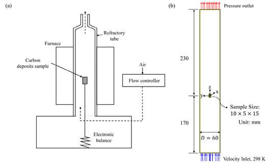
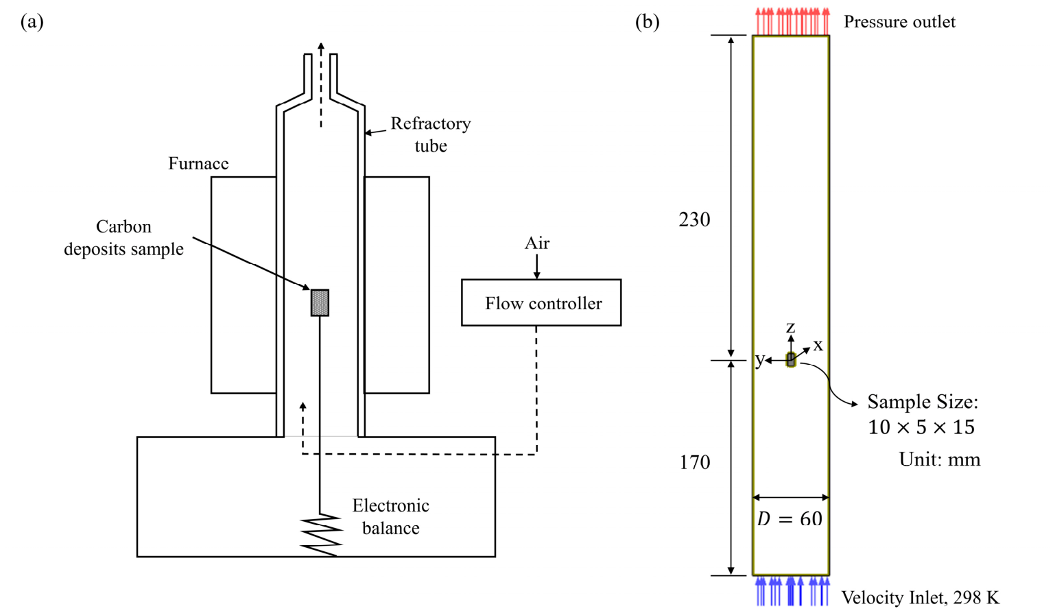
Among the available TG datasets in the literature, those of Zymla and Honnart [16] are particularly well-suited to this study. Their carbon-deposit samples were obtained directly from the walls of an industrial coke oven, so the material properties of the test examples are representative of carbon deposits from the practical coke oven. Their tests were conducted under controlled air flows rather than static air, more closely reproducing the convective environment of the intended application in a coke oven. The TG tube (see Figure 1a) is a vertical cylindrical tube, 400 mm in length ($L$) and 60 mm in diameter ($D$). A rectangular carbon-deposit sample (10 mm ($h$) × 5 mm ($w$) × 15 mm ($l$), as x $\times$ y $\times$ z) is placed within it in the central region, as shown schematically in Figure 1b. The origin of a Cartesian coordinate system is set at the center of the sample. The sample was initially heated to the setting temperature ($T_{ref}$) under an inert nitrogen environment in the TG tube. After temperature stabilization, uniform ambient air at room temperature ($T_{in}$ = 298 K), with a composition of 23.3% $O_2$ and 76.7% $N_2$ by weight, was blown into the TG tube from the bottom to replace the nitrogen. The flue gas was then released as exhaust from the top of the tube.

Figure 1. Schematics of (a) the TG system and (b) the TG tube for the experiment of burning carbon deposits.

Since this study addresses cases of turbulent combustion, only the series conducted under turbulent conditions with the air flow rates ($G$) of 600 and 1000 LPM (equivalent to 0.711 and 1.185 kg/min, respectively) and isothermal conditions (outlet temperatures of 923, 1023, 1123, and 1173 K) in the experiments [16] were selected for this study’s tests. The seven tests are summarized in Table 3, which records the Grashof number (Gr), Reynolds number (Re), and Richardson number (Ri, defined below) for each case.

$$Ri=Gr{Re}^2$$

(2)

Table 3. Flow characterizations in the seven selected TG experiments.

$\mathit{G}$ (kg/min)	${\mathit{T}}_{\mathit{r}\mathit{e}\mathit{f}}$ (K)	$\mathit{G}\mathit{r}$	$\mathit{R}\mathit{e}$	$\mathit{R}\mathit{i}$
0.711	923	$2.31{\times 10}^8$	4028	14.26
	1023	$1.90{\times 10}^8$	3529	15.29
	1123	$1.59{\times 10}^8$	3138	16.17
1.185	923	$2.31{\times 10}^8$	6713	5.13
	1023	$1.90{\times 10}^8$	5881	5.50
	1123	$1.59{\times 10}^8$	5231	5.82
	1173	$1.46{\times 10}^8$	4944	5.97

Here, $Gr$ and $Re$ are defined, respectively, as follows:

$$Gr={\displaystyle \frac{g\beta (T_{out}-T_{in})L^3}{{\upsilon }^2}}$$

(3)

$$Re={\displaystyle \frac{4G}{\pi \upsilon D}}$$

(4)

Here, $\beta$ and $\upsilon$ are evaluated at the mean temperature, $T_{mean}=(T_{in}+T_{out})/2$. Since the $Re$ values for all seven tests exceed 2300, the selected tests in the TG tube fell within the turbulent flow regime. The parameter $Ri$, the ratio of natural to forced convection, identifies the dominant convection type for each test. According to the criterion of Metais and Eckert [34], the $Ri$ values shown in Table 3, ranging from 5.13 to 16.17, indicate a mixed-convection regime in which buoyancy and forced convection are comparably significant. The present validation, covering seven selected tests, was therefore conducted under turbulent, mixed-convection conditions. This contrasts with the laminar, purely forced-convection stagnation flows which are usually considered in past carbon–surface combustion studies in the literature.

3. Problem Modeling and Numerical Aspects

The test problem is a three-dimensional turbulent reacting flow. Solving it requires the conservation equations for continuity, momentum, energy, and species continuity, as well as turbulent transport equations and the equation of state. Heterogeneous chemical reactions occur on the wall surfaces. The molecular-level terms that become dominant in the near-wall subregions must therefore be considered in all equations of the model formulation.

3.1. Modeling Aspects

We recently developed a rigorous formulation for the turbulent carbon-deposit combustion process [28], referred to hereafter as Model 1. This combines the SST k-ω turbulence model, the two-film reaction model for carbon deposits on walls and oxygen in the gaseous mixture, and a beta-shape PDF method that accounts for turbulence–reaction interactions. This PDF method is expressed in terms of the mixture fraction (f, defined below) and its variance (g), each solved from its own transport equation. The mixture fraction is defined by the following:

$$f={\displaystyle \frac{Y_{o_2-}{Y}_{o_{2,air}}}{Y_{o_{2,deposted carbon}-}{Y}_{o_{2,air}}}}$$

(5)

where $Y_{o_2,air}$= 0.233, corresponding to a molar basis of 21% $O_2$ and 79% $N_2$ in air, and $Y_{o_2,depositedcarbon}$ = 0. Equation (5) is thus rewritten as follows:

$$f=1-{\displaystyle \frac{1}{0.233}}{Y}_{o_2},\hspace{1em}\hspace{1em}and\hspace{1em}0\le f\le 1$$

(6)

The mean values of all scalar transport variables (denoted Φ) are calculated by weighting with this assumed-shape function P(f), as follows:

$$\overline{\mathsf{\Phi }}={\int }_0^{1}PDF\left(f\right)\mathsf{\Phi }\left(f\right)df$$

(7)

The beta-shape PDF is expressed as follows:

$$PDF\left(f\right)={\displaystyle \frac{f^{\alpha -1}{(1-f)}^{\beta -1}}{{\int }_0^1{f}^{\alpha -1}{(1-f)}^{\beta -1}df}}$$

(8)

where

$$\alpha =f\left[{\displaystyle \frac{f\left(1-f\right)}{g}}-1\right]$$

(9)

$$\beta =\left(1-f\right)\left[{\displaystyle \frac{f\left(1-f\right)}{g}}-1\right]$$

(10)

The governing equations for all transport variables in Model 1 can be translated into the general form shown below and are summarized in Table 4.

$${\displaystyle \frac{\partial }{\partial t}}\left(\rho \varphi \right)+{\displaystyle \frac{\partial }{\partial xj}}\left(\rho u_j\varphi \right)={\displaystyle \frac{\partial }{\partial xj}}\left({\Gamma }_{\phi }{\displaystyle \frac{\partial }{\partial xj}}\varphi \right)+S$$

(11)

Table 4. Governing transport equations expressed in the general form of Equation (11).

Transport Equation			$\mathsf{\varphi }$	${\mathsf{\Gamma }}_{\mathsf{\varphi }}$	$\mathit{S}$
Continuity			1	$-$	$-$
Momentum			$u_i$	$\mu +{\mu }_t$	${\displaystyle \frac{\partial }{\partial x_j}}\left[(\mu +{\mu }_t)\left(2S_{ij}-{\displaystyle \frac{2}{3}}{\delta }_{ij}{\displaystyle \frac{\partial u_k}{\partial x_k}}\right)-{\displaystyle \frac{2}{3}}\rho {\delta }_{ij}k\right]-{\displaystyle \frac{\partial p}{\partial x_i}}+\rho g_i$
Turbulent kinetic energy			$k$	$\mu +{\sigma }_k{\mu }_t$	$P_k+P_b-\rho {\beta }^{*}k\omega$
Specific turbulent dissipation rate			$\omega$	$\mu +{\sigma }_{\omega }{\mu }_t$	$P_{\omega }+P_b+2\left(1-F_1\right)\rho {\sigma }_{\omega }{\displaystyle \frac{1}{\omega }}{\displaystyle \frac{\partial k}{\partial x_i}}{\displaystyle \frac{\partial \omega }{\partial x_i}}-\rho \widehat{\beta }k{\omega }^2$
Enthalpy			$h$	${\displaystyle \frac{\lambda }{C_p}}+{\displaystyle \frac{{\mu }_t}{{Pr}_t}}$	${\displaystyle \frac{\partial }{\partial x_j}}\left({\sum }_k{h}_k{\overline{\mathcal{J}}}_k\right)+{\displaystyle \frac{Dp}{Dt}}+S_R$
Model 1, Model 2
Species		CO	${\mathrm{Y}}_{CO}$	$\rho D_{m,CO}+{\displaystyle \frac{{\mu }_t}{{Sc}_t}}$	${\displaystyle \frac{\partial }{\partial x_j}}\left({\displaystyle \frac{D_{T,CO}}{T}}{\displaystyle \frac{\partial T}{\partial x_j}}\right)+\overline{R_{CO,4}}$
		CO2	${\mathrm{Y}}_{{CO}_2}$	$\rho D_{{\mathrm{m},\mathrm{C}\mathrm{O}}_2}+{\displaystyle \frac{{\mu }_t}{{Sc}_t}}$	${\displaystyle \frac{\partial }{\partial x_j}}\left({\displaystyle \frac{D_{T,{CO}_2}}{T}}{\displaystyle \frac{\partial T}{\partial x_j}}\right)+\overline{R_{{\mathrm{C}\mathrm{O}}_2,4}}$
Mixture fraction			f	$\rho D_{m,O_2}+{\displaystyle \frac{{\mu }_t}{{Sc}_t}}$	$0.233\left\{-{\displaystyle \frac{\partial }{\partial x_j}}\left({\displaystyle \frac{D_{T,O_2}}{T}}{\displaystyle \frac{\partial T}{\partial x_j}}\right)+\overline{R_{{\mathrm{O}}_2,4}}\right\}$
Variance of mixture fraction			g	$\rho D_{m,O_2}+{\displaystyle \frac{{\mu }_t}{{\sigma }_g}}$	$2\left({\displaystyle \frac{{\mu }_t}{{Sc}_t}}-\mathsf{\rho }{D}_{m,O_2}\right){\displaystyle \frac{\partial f}{\partial x_j}}{\displaystyle \frac{\partial f}{\partial x_j}}-C_d{C}_{\mu }\rho \omega g$
Model 3
Species	CO		${\mathrm{Y}}_{CO}$	$\rho D_{m,CO}+{\displaystyle \frac{{\mu }_t}{{Sc}_t}}$	${\displaystyle \frac{\partial }{\partial x_j}}\left({\displaystyle \frac{D_{T,CO}}{T}}{\displaystyle \frac{\partial T}{\partial x_j}}\right)+\widetilde{R_{CO,4}}$
	CO2		${\mathrm{Y}}_{{CO}_2}$	$\rho D_{{\mathrm{m},\mathrm{C}\mathrm{O}}_2}+{\displaystyle \frac{{\mu }_t}{{Sc}_t}}$	${\displaystyle \frac{\partial }{\partial x_j}}\left({\displaystyle \frac{D_{T,{CO}_2}}{T}}{\displaystyle \frac{\partial T}{\partial x_j}}\right)+\stackrel{~}{R_{{\mathrm{C}\mathrm{O}}_2,4}}$
	O2		${\mathrm{Y}}_{O_2}$	$\rho D_{{\mathrm{m},\mathrm{O}}_2}+{\displaystyle \frac{{\mu }_t}{{Sc}_t}}$	${\displaystyle \frac{\partial }{\partial x_j}}\left({\displaystyle \frac{D_{T,O_2}}{T}}{\displaystyle \frac{\partial T}{\partial x_j}}\right)+\stackrel{~}{R_{{\mathrm{O}}_2,4}}$

The source term SR in the enthalpy equation of Table 4 consists of two contributions, including the heat released by the homogeneous R4 reaction, expressed as follows:

$$R_{reaction}=-\Delta H_4\overline{R_4}$$

(12)

The second contribution is the heat of thermal radiation. Two factors justify treating the radiative field with the P1 model. First, $\mathrm{C}{\mathrm{O}}_2$, a combustion product present in the flow field, makes the field optically thick and diffusive. Second, the radiative field is relatively isotropic, since the carbon-deposit sample is centrally located within a cylindrical configuration. Under these conditions, the P1 radiation transport model [35] is applicable [36]. The heat of thermal radiation is therefore determined using the P1 model, the same one adopted in our previous work [28]. $\overline{R_4}$ in Equation (12) denotes the reaction rate for the homogeneous R4 reaction. It is expressed in terms of the mean values of species mass fraction and temperature, calculated using Equation (15), as follows:

$$\overline{R_4}={\overline{\rho }}^3\overline{k_4} {\overline{Y_{CO}}}^2\overline{Y_{O_2}}$$

(13)

where the mean density ($\overline{\rho }$) and mean rate coefficient ($\overline{k_4}$) are likewise calculated from the mean species mass fractions and temperature. The source terms for the two species mass fractions and the mixture fraction in Table 4 are determined from the stoichiometric relationship:

$$\overline{R_4}=-{\displaystyle \frac{1}{2}}\overline{R_{CO,4}}=-\overline{R_{O_2,4}}={\displaystyle \frac{1}{2}}\overline{R_{C{O}_2,4}}$$

(14)

Information on the formulation of Model 1 can be found in our previous study [28] and is not repeated here.

The rate of reaction R_m for the m-th reaction is expressed as follows:

$$R_m=k_{\mathrm{m}}(T){\rho }^n{\prod }_{k=1}^n{Y}_n^{a_k}$$

(15)

where n is the number of gaseous reactants in the reaction, $a_k$ is the stoichiometric coefficient of the k-th gaseous reactant, and k_m is the reaction-rate coefficient, expressed in Arrhenius form as follows:

$$k_{\mathrm{m}}(T)=A_{m}exp\left(-{\displaystyle \frac{E_m}{R}}{\displaystyle \frac{1}{T}}\right)$$

(16)

The corresponding values of A_m and E_m/R for reactions R1–R4 are summarized in Table 5.

Table 5. Summary of the values of $A$ and $E/R$ shown in the Arrhenius formula, Equation (16), for reactions R1–R4 [23].

Reaction	${\mathit{A}}_{\mathit{m}}\times {10}^{-3}$	$\frac{{\mathit{E}}_{\mathit{m}}}{\mathit{R}}\times {10}^{-4}$ (K)
R1	1.813 $\left(m{s}^{-1}\right)$	1.31
R2	1.225 $\left(m{s}^{-1}\right)$	1.20
R3	7.351 $\left(m{s}^{-1}\right)$	1.66
R4	70.0 $\left(m^3{kg}^{-1}{s}^{-1}\right)$	0.80

The boundary conditions are specified as follows: No-slip conditions are applied at the TG tube wall, with $k_w$ = $g_w$ = 0, $f_w$ = 1 and zero gradients of ω, $Y_{CO}$, and $Y_{C{O}_2}$. The wall temperature is set to the specified isothermal value. No-slip conditions with $k_w$ = $g_w$ = 0, $f_w$ = 1, and zero gradients of ω are also applied on the sample surfaces. The boundary conditions for the $\mathrm{C}\mathrm{O}$ and $\mathrm{C}{\mathrm{O}}_2$ mass fractions and for temperature are instead set from the mass and energy balances of the three heterogeneous reactions, R1 to R3:

$$\mathsf{\rho }{D}_{m,CO}({\displaystyle \frac{d Y_{CO}}{d n}}{)}_{wall}=R_{CO,1}+R_{CO,3}$$

(17)

$$\mathsf{\rho }{D}_{m,C{O}_2}({\displaystyle \frac{d Y_{C{O}_2}}{d n}}{)}_{wall}=R_{C{O}_2,2}+R_{C{O}_2,3}$$

(18)

and

$$-\mathsf{\lambda }{\left({\displaystyle \frac{d T}{d n}}\right)}_{wall}={\displaystyle \sum _{m=1}^3}\Delta H_m{R}_m+q_{r,w}$$

(19)

where $n$ denotes the normal distance from the surface. The radiative boundary condition, $q_{r,w}$, is calculated using the P1 radiation model [36]. Note that $g_w$ = 0 results in PDF($f$) = 1. All reaction rates in Equations (17)$-$(19) are therefore expressed in terms of $\varphi$, since Equation (1) is reduced to $\overline{\varphi }$ = $\varphi$ on the sample surfaces.

The inlet conditions, air at 298 K with $Y_{O_2}$ = 0.233 and $Y_{N_2}$ = 0.767, are assumed to be uniform for all transport variables in Table 4, as follows:

$$u_{in}=u_0\mathrm{and}{v}_{in}=w_{in}=0$$

(20)

$$k_{in}=0.002u_0^2$$

(21)

$${\omega }_{in}=0.1 {\displaystyle \frac{\rho }{\mu }}{k}_{in}$$

(22)

$$f_{in}=g_{in}=0$$

(23)

Zero-gradient conditions are used for all transport variables in Table 4 at the tube outlet, consistent with a fully developed flow state. The initial conditions in the computational domain are a quiescent nitrogen gas atmosphere at the specified temperature.

To compare the one-film and two-film models for turbulent combustion of carbon deposits, the two-film model in Model 1 is replaced by the one-film model. This variant is referred to hereafter as Model 2. All governing equations in Table 4, and the associated boundary and initial conditions, are the same as in Model 1. The only exceptions are the boundary conditions for the $\mathrm{C}\mathrm{O}$ mass fraction and temperature, Equations (17) and (19), which are replaced by the following:

$$\mathsf{\rho }{D}_{m,CO}({\displaystyle \frac{d Y_{CO}}{d n}}{)}_{wall}=R_{CO,1}$$

(24)

$$-\mathsf{\lambda }{\left({\displaystyle \frac{d T}{d n}}\right)}_{wall}=\Delta H_1{R}_1+q_{r,w}$$

(25)

In addition, a zero-gradient boundary condition is set for the $\mathrm{C}{\mathrm{O}}_2$ mass fraction, since no $\mathrm{C}{\mathrm{O}}_2$ is produced by the one-film model on the sample surfaces.

Hang et al. [24] and Chung and Chang [28] used two different models for turbulence–reaction interactions. To compare their predictions, the beta-shape PDF method of Equation (8), used in Model 1 to represent turbulent fluctuations, is replaced here by the eddy-dissipation model used by Hang et al. [24]. This variant is referred to hereafter as Model 3.

The mean reaction rate for the homogeneous R4 reaction using the eddy-dissipation model is determined by the following [31]:

$$\widetilde{R_4}=min(R_{EBU},R_4)$$

(26)

$$R_4={\rho }^3{k}_4 Y_{CO}^2 Y_{O_2}$$

(27)

$$R_{EBU}=\mathsf{\rho }({\displaystyle \frac{\epsilon }{k}})A_{4}min\left({\displaystyle \frac{Y_{CO}}{{\upsilon }_{CO}^{\prime }}},{\displaystyle \frac{Y_{O_2}}{{\upsilon }_{O_2}^{\prime }}},{\displaystyle \frac{Y_{C{O}_2}}{{\upsilon }_{C{O}_2}^{″}}}\right)$$

(28)

Here, the stoichiometric coefficients for the homogeneous R4 reaction on a mass basis are defined by the following:

$${\upsilon }_{CO}^{\prime }\mathrm{C}{\mathrm{O}}_{\left(\mathrm{g}\right)}+{\upsilon }_{O_2}^{\prime }{\mathrm{O}}_{2\left(\mathrm{g}\right)}\to {\upsilon }_{{CO}_2}^{″}\mathrm{C}{\mathrm{O}}_{2\left(\mathrm{g}\right)}$$

(29)

Setting the $\mathrm{C}\mathrm{O}$ coefficient to 1 gives an ${\mathrm{O}}_2$ coefficient of 0.572 and a $\mathrm{C}{\mathrm{O}}_2$ coefficient of 1.572. The original eddy-dissipation model was developed with the k-ε turbulence model. Introducing the transformation $\epsilon /k=C_{\mu }\omega$ into Equation (28) gives the following:

$$R_{EBU}=\mathsf{\rho }{C}_{\mu }\omega A_{4}min\left({\displaystyle \frac{Y_{CO}}{1}},{\displaystyle \frac{Y_{O_2}}{0.572}},{\displaystyle \frac{Y_{C{O}_2}}{1.572}}\right)$$

(30)

While using the eddy-dissipation model, the reaction rate for each species follows the stoichiometric relationship for R4:

$$\widetilde{R_4}=-{\displaystyle \frac{1}{2}}\widetilde{R_{CO,4}}=-\widetilde{R_{O_2,4}}={\displaystyle \frac{1}{2}}\widetilde{R_{C{O}_2,4}}$$

(31)

Model 3 therefore requires no transport equations for f and g. Instead, a transport equation for the ${\mathrm{O}}_2$ mass fraction is solved together with those for $\mathrm{C}\mathrm{O}$ and $\mathrm{C}{\mathrm{O}}_2$, as shown in Table 4. The boundary and initial conditions are all the same as those used in Model 1.

3.2. Numerical Aspects

The governing equations in Table 4 can be solved using the CFD code ANSYS 2024 R2 [37]. The convective and diffusion terms are discretized using the second-order upwind and central schemes, respectively. The SIMPLEC algorithm [38] accounts for velocity–pressure coupling in the momentum equations. The time-derivative term is discretized using the first-order implicit scheme. A time step of 5 × 10⁻⁴ s is used, which is much smaller than the reaction time scales for R1 to R4 (about 8 × 10⁻⁴ s or greater). This avoids the numerical stiffness that would otherwise arise from the fast chemical kinetics of the present reactions. At each time step, the convergence criterion requires the residuals of all solved transport variables in the computational domain to reach their own asymptotic values.

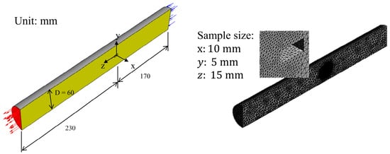
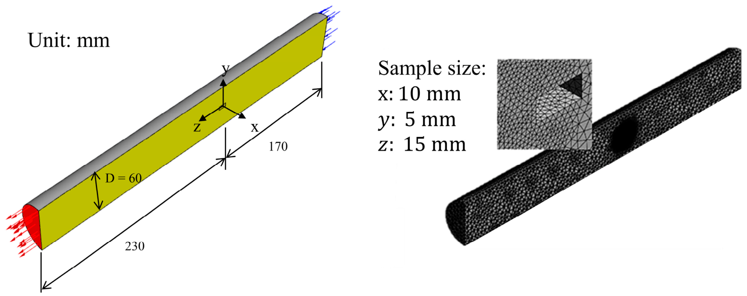
Figure 2 shows the employed computational domain and mesh for the TG tube. The tube dimensions and the inlet (blue arrows) and outlet (red arrows) boundaries are shown with a magnified view of the surface mesh. This is locally refined in the subregion near the carbon-deposit sample to resolve steep near-wall gradients of flow properties induced by the heterogeneous surface reactions.

Figure 2. Computational domain and mesh of the TG tube with a magnified view of the locally refined surface mesh near the carbon-deposit sample.

A grid independence test is performed using three meshes, coarse, medium, and dense, containing 74,508, 124,180, and 163,918 grid cells, respectively. For all three meshes, the first grid points from the surfaces are positioned to satisfy $y_p^{+}$ < 2, ensuring that they fall within the viscous sublayer of the boundary layer. The mean combustion rate ($\overline{r_s}$), defined below, is used to assess prediction accuracy in the grid independence test.

$$r_s=-{\displaystyle \frac{1}{A}}{\displaystyle \frac{dm}{dt}}={\sum }_{m=1}^3{R}_{m}dA$$

(32)

$$\overline{r_s}={\displaystyle \frac{1}{t_{2-t_1}}}{\int }_{t_1}^{t_2}{r}_{s}dt$$

(33)

The method used to determine the mean combustion rate is discussed in the next section. Table 6 summarizes the results for the grid independence test. Here, the relative difference, calculated with respect to the dense-mesh result, decreases asymptotically to a near-negligible value. Although the medium mesh already agrees with the dense-mesh result to within 0.868%, well within an acceptable tolerance, the dense mesh was retained for all subsequent computations to better resolve the localized gradients of species and temperature near the sample (reacting) surfaces.

Table 6. Grid independent tests for the case at $T_{out}=1123\mathrm{K}$ and $G=1.185\mathrm{k}\mathrm{g}/\mathrm{m}\mathrm{i}\mathrm{n}$.

Mesh Elements	Mean Combustion Rate ($\overline{{\mathit{r}}_{\mathit{s}}}$) ($\frac{\mathbf{g}}{{\mathbf{c}\mathbf{m}}^2\mathbf{s}}\times {10}^{-4}$)	Relative Error on Base of Dense Grid Case (%)
74,508	$1.303$	3.742
124,180	$1.245$	0.868
163,918	$1.256$	$-$

4. Results and Discussion

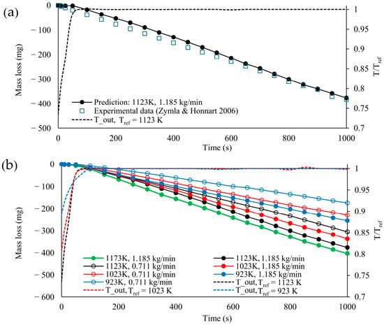
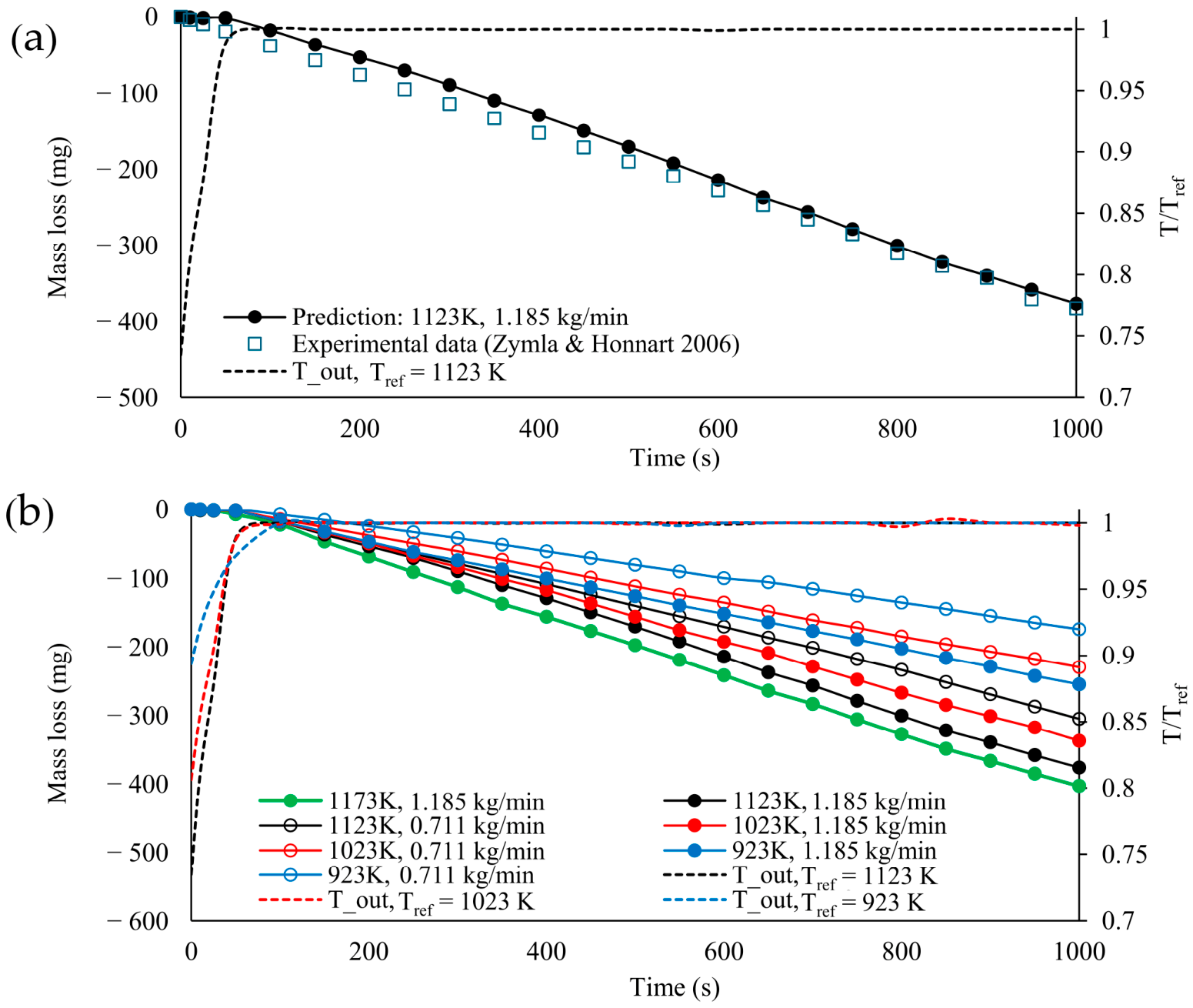
The combustion of the carbon-deposit sample in the TG tube occurred in three stages. In the first stage, nitrogen was replaced by ambient air, and ignition occurred. In the second stage, the combustion rate remained nearly steady, and in the third, the sample approached burnout, and the combustion rate gradually slowed. The test at an air flow rate of 1.185 kg/min and a temperature of 1123 K is taken as a representative example to illustrate this process. Model 1 was used for the simulation. Figure 3a shows the predicted mass loss of the carbon deposit versus time, from ignition to 1000 s, and the experimental results of Zymla and Honnart [16] for comparison. The dotted curve in Figure 3a represents rapid heating to the set outlet temperature of 1123 K for this isothermal test. The experimental data were recorded from the onset of combustion in the experiments of Zymla and Honnart, that is, from the ignition phase.

Figure 3. (a) Validation of isothermal TG simulation for cases at 1123 K and 1.185 kg/min, and (b) predicted mass loss curves for all cases in the preheating and nearly steady combustion stages.

Mianowski et al. [15] found that the reaction rate coefficient at the point of initial oxidation depends on the ignition temperature and should be expressed using a three-parameter function:

$$k_{\mathrm{m}}\left(T\right)=A_m{T}^{{\alpha }_m}exp\left(-{\displaystyle \frac{E_m}{R}}{\displaystyle \frac{1}{T}}\right)$$

(34)

Accurate simulation of the ignition phase therefore requires a three-parameter kinetic function of this kind. However, three-parameter rate coefficients for the three heterogeneous reactions (R1 to R3) are not available in the literature. Instead, the present simulation uses the two-parameter Arrhenius formulation in Equation (15) and Table 5 for the entire combustion process, including the ignition phase. As a result, the predicted mass loss is slightly overestimated for a period of time after the initial oxidation, compared with the experimental data.

Zymla and Honnart observed that the mass loss rate became nearly invariant; that is, one stage had a nearly constant combustion rate at about 10 min after ignition, which lasted about 35 min before the sample reached complete combustion (see their Figure 14 in [16]). The predicted mass loss fits the experimental data well at t > 600 s for the stage of nearly invariant mass loss rate. Only a portion of the results, up to 1000 s, is shown in Figure 3a. The values of $t_1$ and $t_2$ used to calculate the mean combustion rate in Equation (33) are set to 600 s and 1000 s, respectively, in this study. Figure 3b shows the combustion processes predicted using Model 1 for all seven selected tests (Table 3). Two trends are apparent, as shown in Figure 3b. The mean combustion rate of carbon deposits increases with a higher air flow rate or a higher outlet temperature.

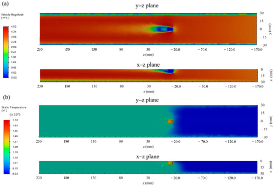
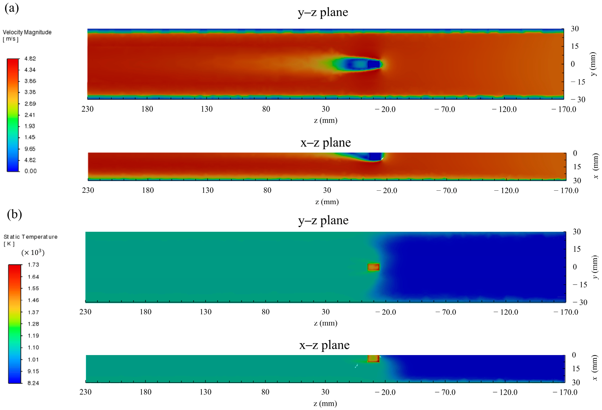
Figure 4a,b show the stream-wise velocity and temperature distributions in the TG tube, plotted from two view angles at t = 800 s, representing the nearly steady combustion stage. High temperatures are distributed around the sample and, in turn, produce a flow region that causes significant buoyancy downstream of the sample. This corroborates the earlier characterization, based on the $Ri$ number, of a turbulent flow with a mixed pattern of forced and free convection.

Figure 4. Distribution of (a) stream-wise velocity and (b) temperature in the TG tube for cases at 1123 K and 1.185 kg/min at 800 s.

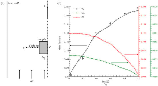
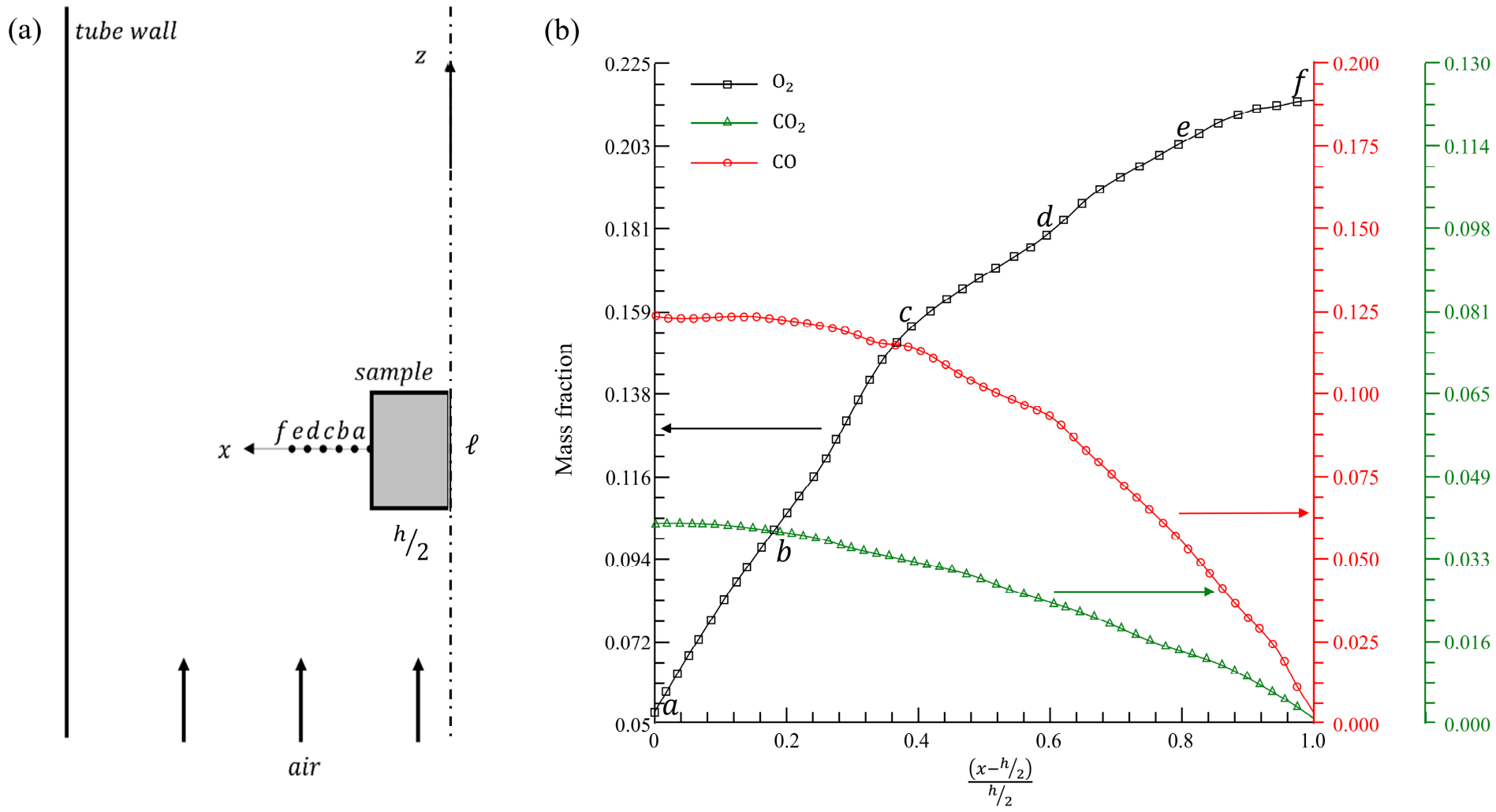
Figure 5 illustrates the mass fraction distributions of three species, $O_2$, $CO$, and $C{O}_2$, along the x-axis close to the sample surface on planes y = 0 and z = 0 at t = 800 s. The mass fraction scales in Figure 5b differ for each species. According to the two-film reaction model, $CO$ is produced through the two heterogeneous reactions R1 and R3, while $C{O}_2$ is produced through R2 and consumed simultaneously through R3. As a result, the $CO$ mass fractions in Figure 5b are higher than those of $C{O}_2$.

Figure 5. (a) Illustration of 6 selective locations in TG tube and (b) sectional distributions of mass fraction for three species obtained with Model 1.

To examine the effect of turbulence–reaction interactions, Table 7 records the $O_2$ mass fractions at six selected locations along the x-axis close to the sample surface, on planes y = 0 and z = 0, at t = 800 s (see Figure 5a). These values, obtained directly from the $O_2$ transport equation, are compared with the mean values obtained from Equation (7) using the beta-PDF. The two values differ except at location f, which is adjacent to the free air stream, though these differences are not significant. They are equal at location $f$ because this location lies in a region where no chemical reaction occurs.

Table 7. Comparison of mass fractions of oxygen with and without the PDF model at six selected locations for cases at 1123 K and 1.185 kg/min.

Location	${\mathit{Y}}_{{\mathit{O}}_2}$	$\mathit{f}$	$\mathit{g}$	$\mathit{\alpha }$	$\mathit{\beta }$	$\overline{{\mathit{Y}}_{{\mathit{O}}_2}}$
point a	0.00049	0.9979	0.0001	19.944	0.042	0.00047
point b	0.080	0.6567	0.001	147.392	77.068	0.079
point c	0.151	0.3562	0.0034	23.671	42.779	0.150
point d	0.170	0.2704	0.0061	8.532	23.022	0.174
point e	0.211	0.0987	0.0005	17.466	159.471	0.212
point f	0.232	0.0043	0.0004	0.042	9.642	0.232

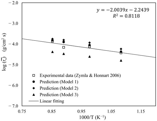
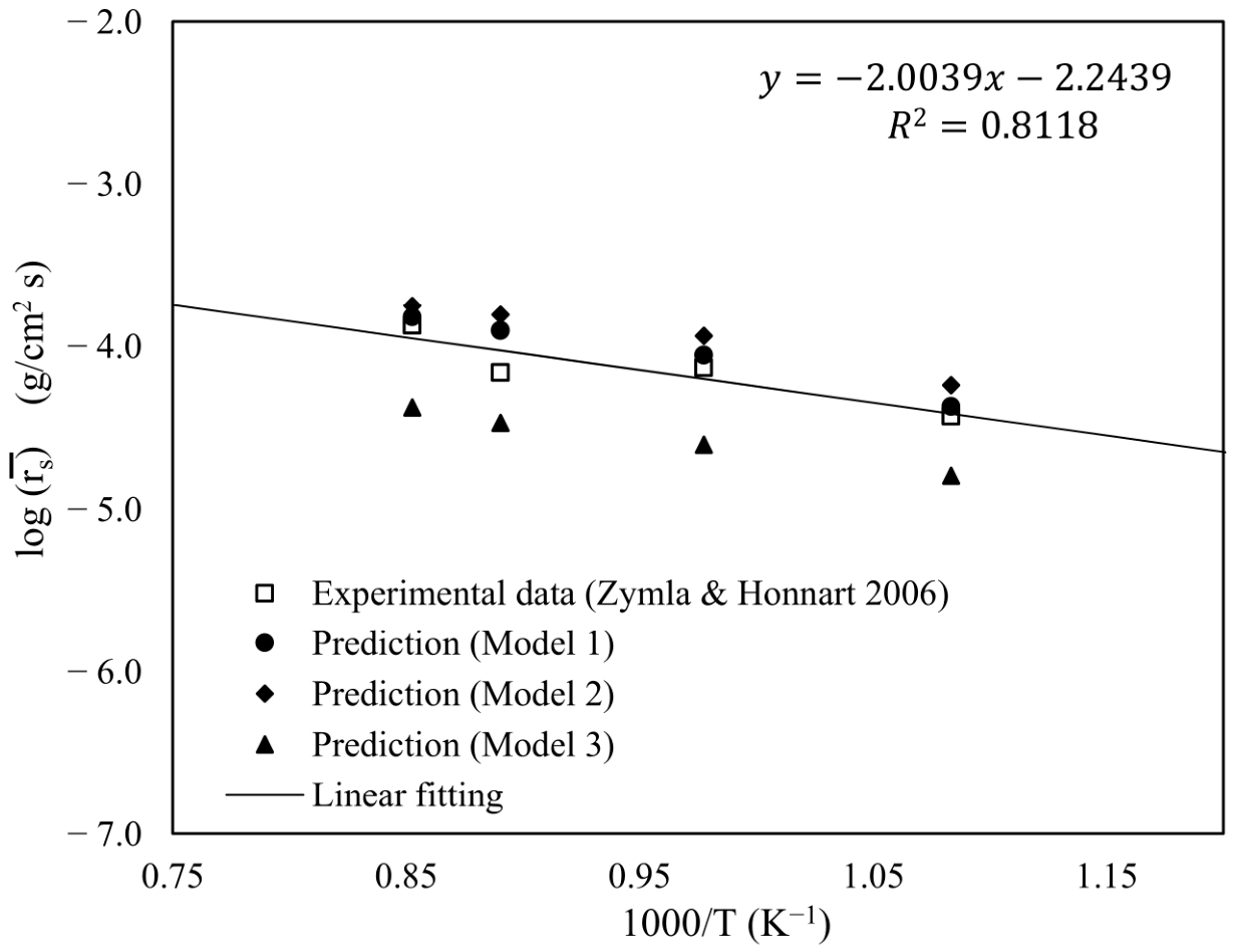
Table 8 and Figure 6 compare the mean combustion rates predicted by Model 1, calculated using Equations (32) and (33), against the available experimental data from a turbulent flow regime in the study of Zymla and Honnart [16]. Four isothermal temperatures (923, 1023, 1123, and 1173 K) were used with an air flow rate of 1.185 kg/min. The comparison shows good agreement between the Model 1 predictions and the experimental data, with the deviation for each case remaining below 3.5% (see Table 8).

Table 8. Comparison of the predicted combustion rates using Model 1 with experimental data [16].

Temperature (K)	Experimental Combustion Rate ($\frac{\mathbf{g}}{{\mathbf{c}\mathbf{m}}^2\mathbf{s}}$)	Predicted Combustion Rate ($\frac{\mathbf{g}}{{\mathbf{c}\mathbf{m}}^2\mathbf{s}}$)	Percentage Difference * (%)
923	$-$4.415	$-$4.371	$-$0.996
1023	$-$4.203	$-$4.056	$-$3.497
1123	$-$4.028	$-$3.905	$-$3.054
1173	$-$3.952	$-$3.821	$-$3.315

* difference = $\left[\left({\displaystyle \frac{prediction}{experimentaldata}}\right)-1\right]\times 100\%.$

Figure 6. Comparison between the experimental data and the predicted mean combustion rates using the three investigated models for the cases with a flow rate of 1.185 kg/min.

The same four tests, at a flow rate of 1.185 kg/min, were re-simulated using Model 2, which replaces the two-film reaction model with the one-film model to examine the effect of the reaction model on the predictions. These results are presented in Figure 6. The one-film model appears to underpredict the combustion rate in the temperature range investigated compared to the experimental data. This shows that the two-film reaction model should be used to correctly predict the combustion of carbon deposits. Adomeit et al. [19] used the ratio ($r_{\tau }$) between the residence time for the homogeneous reaction (R4) within the boundary layer of mass transport and its reaction time to justify which chemical reaction model (one-film or two film) would perform better for the combustion of carbon deposits. When the ratio is greater than unity, it favors the two-film model; otherwise, it favors the one-film model. The sectional profile for CO in Figure 5b for the case at 1123 K and1.185 kg/min of air flow rate was used to estimate this ratio as an example. The boundary layer for mass transport on the sample surface along the x axis is defined from the surface $\left(x={\displaystyle \frac{h}{2}}\right)$ to the position $x_0$ where $y_{CO}$/$y_{CO,max}=5\%$. Based on this definition, $x_0={\displaystyle \frac{h}{2}}+0.454h$, as located in Figure 5a, and the all six points (a–f) marked in Figure 5a are located within the boundary layer. Values of ${\mu }_t$/$\mathsf{\mu }$ were in the range 3–10 for the points from b to f marked in Figure 5a, indicating that it is indeed a turbulent boundary layer. At the point of a in Figure 5a, ${\mu }_t$/$\mathsf{\mu }$ $\approx 0.$4, implying that this point is located in the buffer zone of the boundary layer since O(${\mu }_t)$ = O($\mathsf{\mu }$). Note that the first grid was placed with the condition of $x_p^{+}<2$ in the computational mesh.

Evaluation of $r_{\tau }$ can be approximated as:

$$r_{\tau }={\displaystyle \frac{r_s}{J}}$$

(35)

where J is the turbulent mass diffusive flux of CO species shown in Table 4; that is, J = ${\displaystyle \frac{{\mu }_t}{{Sc}_t}}$ ${\displaystyle \frac{\partial Y_{CO}}{\partial x}}$. J values can be estimated with $J\approx (\mu ₜ/Scₜ)(\Delta Yco/\Delta x)$, where $Scₜ=0.7$ is the turbulent Schmidt number, for the segments of b–c, c–d, d–e, and e–f, with the result of $Y_{CO}$ recorded in Figure 5b. The corresponding combustion rate of carbon deposits is r_s = 39.05 kg/(m²·s (see Table 8). The calculated results are tabulated below.

All the estimated $r_{\tau }$ values in Table 9 are much greater than unity. According to the criterion of Adomeit et al. [19], the two-film model would be superior than the one-film model in the present tested case. The results shown in Table 9 help interpret why the predictions using the two-film model were better than those using the one-film model, as shown in Figure 6.

Table 9. Summary of $r_{\tau }$ values estimated at four segments.

Segment	Δ${\mathbf{Y}}_{\mathbf{C}\mathbf{O}}$	Δ${\mathbf{Y}}_{\mathbf{C}\mathbf{O}}$/Δx (m−1)	J (kg/(m2·s))	${\mathbf{r}}_{\mathbf{s}}$/J = ${\mathit{r}}_{\mathit{\tau }}$
b → c	0.0079	158	0.0226	1730.1
c → d	0.0219	438	0.0626	624.1
d → e	0.0394	788	0.1126	346.9
e → f	0.0498	996	0.1423	274.4

The same four tests were re-simulated using Model 3, which replaces the beta-shape PDF with the eddy-dissipation model (EDM) to account for turbulence–reaction interactions. Predictions of the mean combustion rate are shown in Figure 6. The EDM overpredicts the combustion rate in the investigated temperature range compared with the experimental data. This result makes sense because the EDM was developed under an assumption of a premixed flame; in other words, a mixed-is-burned approximation. However, the present problem uses a diffusion-dominant flame. The beta-shape PDF model is therefore more appropriate than the EDM for representing turbulence–reaction interactions in this study.

The four experimental combustion rates recorded in Table 8 are correlated with temperature by the following function:

$$log\left(\overline{r_s}\right)=-2.0039\left({\displaystyle \frac{1000}{T}}\right)-2.2439$$

(36)

The coefficient of determination ($R^2$) for this fit is 0.8118, indicating good agreement between the experimental data and the correlation. The correlation curve is also plotted in Figure 6.

To quantify the goodness of fit for all data in Figure 6, root-mean-square errors (RMSEs) were calculated relative to Equation (36) for the experimental data [16] and for the predictions of Models 1, 2, and 3. These values are recorded in Table 10. To some extent, the RMSE of experimental data can be regarded as a measure of experimental uncertainty. As a result, Model 1’s RMSE falls within the experimental uncertainty range reported by Zymla and Honnart [16], supporting Model 1’s good predictive performance for carbon-deposit combustion in air.

Table 10. Comparison of the root-mean-square deviations based on the fitting correlation for the experimental data and the various combustion models used to simulate TG tube experiments with ${\displaystyle \frac{1000}{T}}$ = 0.853 $-$ 1.083 (${\mathrm{K}}^{-1}$).

	Experimental Data [5]	Predictions
		Model 1	Model 2	Model 3
RMSE	0.121	0.106	$0.216$	0.177

5. Conclusions

The air injection technique is becoming widely adopted to remove carbon deposits in coke-oven operations [4,5,6,7,8,9,10,11,12,13]. A physical model for simulating the turbulent reacting flow of this carbon-deposit removal process is necessary for numerical analysis. However, there is a lack of in situ measurement data available for the removal rate of carbon deposits via air injection in practical coke ovens. Thus, benchmark data obtained from turbulent flow regimes performed in TG experiments in the literature were used to validate the comprehensive turbulent combustion model developed in this study.

Three models were examined. Considering heterogeneous reactions occurring on the surface of the FC sample, the SST k-$\omega$ turbulence model was employed in all three tested models to ensure accurate near-wall predictions of flow properties. After comparing this with the performances of Model 2, which employs the one-film model for carbon–air reactions together with a beta-shape PDF method to account for turbulence–reaction interactions, and Model 3, which employs the EDM method to account for turbulence–reaction interactions with the two-film model for carbon–air reactions, Model 1, which employs both the two-film model and a beta-shape PDF method, was found capable of simulating the turbulent combustion tests of carbon-deposit samples in the benchmarked TG experiments.

This model can simulate carbon deposit removal in coke ovens through air injection.

References

- Nakagawa, K.; Kato, K.; Naito, T. Growth rate of carbon deposit by pyrolysis reaction of carbonization gas. In Proceedings of the International Congress on the Science and Technology of Ironmaking (ICSTI), Osaka, Japan, 26–30 November 2006; pp. 406–409. Available online: https://www.researchgate.net/publication/242736865_Carbon_Deposition_Mechanism_in_Coke_Oven_Chamber_Influence_of_Fine_Particles_on_Formation_Rate_of_Carbon_Deposits (accessed on 29 July 2026).
- Sugiura, M.; Nakagawa, T.; Arima, T.; Kato, K.; Sakaida, M.; Morizane, Y.; Sano, A.; Irie, K. Quantitative influence of coke oven wall irregularity on pushing force. ISIJ Int. 2013, 53, 583–589. [Google Scholar] [CrossRef] [Scilit]
- Abe, Y.; Sugiura, M. Behavior of carbon adhesion on aged coking-chamber walls to pushing load. ISIJ Int. 2022, 62, 64–73. [Google Scholar] [CrossRef] [Scilit]
- Takahashi, T.; Uchida, T.; Matsuda, K. Clearing Apparatus for Deposited Carbon in Carbonizing Chamber of Coke Oven. Japan Patent JP2561787B2, 11 December 1996. [Google Scholar]
- Ota, Y.; Okanishi, K.; Kikuchi, A. Removal of Carbon Attached to Space Part at Top of Furnace of Carbonizing Chamber of Coke Oven. Japan Patent JP3247288B2, 15 January 2002. [Google Scholar]
- Suzuki, K.; Nakamura, O.; Shinohara, K. Lance for Burning to Remove Carbon in Carbonizing Chamber of Coke Oven. Japan Patent JP4760388B2, 31 August 2011. [Google Scholar]
- Oishi, H.; Ishioka, M. Method for Removing Adhered Carbon in Carbonization Chamber of Coke Oven. Japan Patent JP4736400B2, 27 July 2011. [Google Scholar]
- Fukazawa, Y.; Koga, M.; Tsutsumi, T.; Ito, K.; Sakai, K. Method for Incinerating Carbon Attached to Coke Oven Carbonization Chamber. Japan Patent JP4676875B2, 27 April 2011. [Google Scholar]
- Nakamura, T. Method of Burning Removal of Deposit Carbon in Carbonization Chamber of Coke Oven. Japan Patent JP6278185B2, 14 February 2018. [Google Scholar]
- Umeda, K. Method of Removing Adhered Carbon on Furnace Wall of Coking Chamber During Operation of Coke Oven. Japan Patent JP6769225B2, 14 October 2020. [Google Scholar]
- Wang, D.H.; Wu, Y.L. Method for Burning-Off Deposited Carbon Inside Coke Oven. Taiwan Patent TWI762408B, 21 April 2022. [Google Scholar]
- Yoshimori, Y.; Yatsugayo, K.; Takeo, S.; Ikemoto, S. Deposit Carbon Removal Method in Coke Oven Carbonization Chamber. Japan Patent JP2024016577A, 7 February 2024. [Google Scholar]
- Quanci, J.F.; Charles, D.C.; West, G.D.; Evatt, S.; Ball, M.A.; Crum, J.F. Decarbonization of Coke Ovens and Associated Systems and Methods. U.S. Patent US12305119B2, 20 May 2025. [Google Scholar]
- Vyazovkin, S.; Chrissafis, K.; Di Lorenzo, M.L.; Koga, N.; Pijolat, M.; Roduit, B.; Sbirrazzuoli, N.; Suñol, J.J. ICTAC Kinetics Committee recommendations for collecting experimental thermal analysis data for kinetic computations. Thermochim. Acta 2014, 590, 1–23. [Google Scholar] [CrossRef] [Scilit]
- Mianowski, A.; Bigda, R.; Zymla, V. Study on kinetics of combustion of brick-shaped carbonaceous materials. J. Therm. Anal. Calorim. 2006, 84, 563–574. [Google Scholar] [CrossRef] [Scilit]
- Zymla, V.; Honnart, F. Coke oven carbon deposits growth and their burning off. ISIJ Int. 2007, 47, 1422–1431. [Google Scholar] [CrossRef] [Scilit]
- Krebs, V.; Marêché, J.F.; Furdin, G.; Dumay, D. Contribution to the study of carbon deposition in coke ovens. Fuel 1994, 73, 1904–1910. [Google Scholar] [CrossRef] [Scilit]
- Turns, S.R. An Introduction to Combustion: Concepts and Applications, 3rd ed.; McGraw-Hill: New York, NY, USA, 2012. [Google Scholar]
- Adomeit, G.; Hocks, W.; Henriksen, K. Combustion of a carbon surface in a stagnation point flow field. Combust. Flame 1985, 59, 273–288. [Google Scholar] [CrossRef] [Scilit]
- Gao, Z.H.; Xu, J.J.; Qian, Y.H.; Li, M.S. Effects of surface temperature, flow velocity and ambient pressure on the oxidation of graphite at 1400–2000 °C in O2. Corros. Sci. 2014, 78, 269–275. [Google Scholar] [CrossRef] [Scilit]
- Shaddix, C.R. An improved semi-global intrinsic kinetics model for high temperature carbon oxidation. Proc. Combust. Inst. 2024, 40, 105339. [Google Scholar] [CrossRef] [Scilit]
- Yi, F.; Fan, J.; Ki, D.; Lu, S.; Luo, K. Three-dimensional time-dependent numerical simulation of a quiescent carbon combustion in air. Fuel 2011, 90, 1522–1528. [Google Scholar] [CrossRef] [Scilit]
- Gu, M.; Chen, G.; Zhang, M.; Huang, D.; Chaubal, P.; Zhou, C.Q. Three-dimensional simulation of the pulverized coal combustion inside blast furnace tuyere. Appl. Math. Model. 2010, 34, 3536–3546. [Google Scholar] [CrossRef] [Scilit]
- Hang, J.G.; Chang, K.C.; Hsu, U.K.; Wang, D.H. Feasibility study of burning-off carbon deposits in coke oven by means of air injection process. J. Chin. Soc. Mech. Eng. 2015, 36, 233–240. Available online: https://www.researchgate.net/publication/283425528_Feasibility_Study_of_Burning-Off_Carbon_Deposits_in_Coke_Oven_by_Means_of_Air_Injection_Process (accessed on 29 July 2026).
- Wang, D.H.; Chuang, Y.W.; Tsai, C.H. The simulation of burning-off the deposited carbon in a coke oven. China Steel Technol. Rep. 2017, 30, 12–19. [Google Scholar]
- Shih, T.H.; Liou, W.W.; Shabbir, A.; Yang, Z.; Zhu, J. A new k-ε eddy viscosity model for high Reynolds number turbulent flows. Comput. Fluids 1995, 24, 227–238. [Google Scholar] [CrossRef] [Scilit]
- Jongen, T. Simulation and Modeling of Turbulent Incompressible Flows. Ph.D. Thesis, École Polytechnique Fédérale de Lausanne, Lausanne, Switzerland, 1995. [Google Scholar]
- Chung, Y.D.; Chang, K.C. Aspects on numerical modeling of the burning-off process for the removal of deposited carbon in a coke-oven chamber. J. Aeronaut. Astronaut. Aviat. 2024, 56, 857–878. [Google Scholar] [CrossRef]
- Menter, F.R. Two-equation eddy-viscosity turbulence models for engineering applications. AIAA J. 1994, 32, 1598–1605. [Google Scholar] [CrossRef] [Scilit] [PubMed]
- Jones, W.P.; Whitelaw, J.H. Modeling and measurements in turbulent combustion. Symp. Int. Combust. 1984, 20, 233–249. [Google Scholar] [CrossRef] [Scilit]
- Magnussen, B.F.; Hjertager, B.H. On mathematical modeling of turbulent combustion with special emphasis on soot formation and combustion. Symp. Int. Combust. 1977, 16, 719–729. [Google Scholar] [CrossRef] [Scilit]
- Pope, S.B. PDF methods for turbulent reacting flows. Prog. Energy Combust. Sci. 1985, 11, 119–192. [Google Scholar] [CrossRef] [Scilit]
- Soong, H.C.; Chang, K.C. Examination of interaction between turbulence and combustion in diffusion flame. Int. J. Turbo Jet-Engines 1992, 9, 227–238. [Google Scholar] [CrossRef] [Scilit]
- Metais, B.; Eckert, E.R.G. Forced, mixed, and free convection regimes. J. Heat Transf. 1964, 86, 295–296. [Google Scholar] [CrossRef] [Scilit]
- Larsen, E.W.; Thömmes, G.; Klar, A.; Seaïd, M.; Götz, T. Simplified PN approximations to the equations of radiative heat transfer and applications. J. Comput. Phys. 2002, 183, 652–675. [Google Scholar] [CrossRef] [Scilit]
- Howell, J.R.; Siegel, R.; Mengüç, M.P. Thermal Radiation Heat Transfer, 5th ed.; CRC Press: Boca Raton, FL, USA, 2011. [Google Scholar] [CrossRef] [Scilit]
- ANSYS Inc. ANSYS Fluent User’s Guide, Release 2024 R2; ANSYS, Inc.: Canonsburg, PA, USA, 2024. [Google Scholar]
- Van Doormaal, J.P.; Raithby, G.D. Enhancements of the SIMPLE method for predicting incompressible fluid flows. Numer. Heat Transf. 1984, 7, 147–163. [Google Scholar] [CrossRef] [Scilit]
Disclaimer/Publisher’s Note: The statements, opinions and data contained in all publications are solely those of the individual author(s) and contributor(s) and not of MDPI and/or the editor(s). MDPI and/or the editor(s) disclaim responsibility for any injury to people or property resulting from any ideas, methods, instructions or products referred to in the content. |
© 2026 by the authors. Licensee MDPI, Basel, Switzerland. This article is an open access article distributed under the terms and conditions of the Creative Commons Attribution (CC BY) license.