Physics-Informed Neural Networks for Dissipative Micropolar Nanofluid Flow with Microrotation Dynamics and Zero Nanoparticle Mass Flux

Abstract

This research presents a physics-informed deep learning framework for investigating the magnetohydrodynamic flow of a dissipative non-Newtonian micropolar nanofluid induced by a stretching sheet, incorporating Stefan blowing, internal heat generation, and the zero nanoparticle mass flux condition. The physical model consists of the interplay between the microrotation dynamics, resistance of porosity on the microrotation, Brownian diffusion, and thermophoretic transport phenomenon. The numerical solutions for the nonlinear yielded equations that result from the above interaction are obtained by employing a PINN that considers the laws of physics and boundary conditions. With this technique, the flow behavior, temperature, concentration, and microrotation fields can be predicted accurately without requiring huge datasets. This shows the ability of PINNs to numerically treat highly-coupled nonlinear transport equations in a very efficient manner compared to other traditional methods. The important discoveries from this study include that the porous and magnetic factors increased the skin friction coefficient, but the magnetic effect and viscous dissipation decreased the rate of heat transfer, and the thermophoresis effect decreased the rate of mass transfer while the Brownian effect increased it. The precision of the PINN algorithm is confirmed by comparison of the results with the earlier findings, which proves very high accuracy and hence the robustness of the current computing framework. Results of this research are useful for the development of some thermal management systems, energy converters, cooling methods, chemical reaction processes, fuel cell technology, porous media reactors, and ocean engineering involving the transport of complicated non-Newtonian nanofluids.

1. Introduction

The micropolar nanofluids belong to an advanced category of non-Newtonian fluids that consist of nanofluid particles in a micropolar fluid, wherein the microstructure of the fluid influences the flow behavior of the fluid. The micropolar nanofluids are different from the traditional nanofluids in the sense that they consider the rotational degree of freedom of the micro-elements present in the fluid. Therefore, micropolar nanofluids have high potential in modeling various rheological phenomena, because of their increased thermal conductivity, higher heat transfer rate, and microrotation features. Thus, micropolar nanofluids possess immense importance in many fields of engineering because of their unique properties. Micropolar nanofluids have enormous importance in many maritime applications such as thermal management of ships propulsion, heat transfer of submarine equipment, and heat exchanger design for offshore structures. They can also be used in engineering devices such as biomedical devices, electronics cooling system, nuclear reactors, and energy harvesters. There have been several contributions to the field in the recent past. Tayebi et al. [1] analyzed thermal free convection and entropy generation for micropolar nanofluid flow in an inclined I-shape enclosure with two heated cylinders, which is very important to understand the effects of buoyancy-induced flow and thermodynamic irreversibility. Bhatti and Zafar [2] studied the effects of combined Dufour and Soret on MHD micropolar nanofluid flow in presence of heat source and nonlinear radiation, making further contributions to understand the mass and heat transport processes. Ahmad and Jamil [3] considered heat transfer analysis in a Darcy-Forchheimer porous medium with thermal radiation, showing the effect of interaction between porosity and radiation effect. Chaudhary and Khan [4] analyzed the thermal performance of micropolar nanofluid in a porous channel with variable thermal conductivity. The researchers Farooq and Ahmed [5] have provided a numerical simulation for the micropolar nanofluid over a porous sheet considering the influence of viscous dissipation and radiation, thereby showing significant improvements in thermal performance for these cases. Very recently, the researchers Thabet et al. [6] performed a detailed numerical analysis for the case of MHD micropolar nanofluid over an inclined surface considering the effects of thermophoresis, Brownian motion, and thermal performance.

The Stefan blowing process is the mass transfer based phenomenon of transpiration which occurs because of the creation of normal flow due to diffusion of species at the interface. As compared to the injection and suction processes, Stefan blowing happens naturally due to the concentration gradients, and hence, this process has immense importance for coupled heat and mass transport phenomena. The process can be observed in many practical cases like evaporation and condensation processes, drying systems, fuel cells, coating processes, polymerization, etc. The phenomenon of Stefan blowing has been investigated widely in the field of nanofluids. Manjunatha et al. [7] have investigated the joint role of Stefan blowing, convective heating, and chemical reaction on the flow of nanofluid over a curved stretching surface, where it is clearly seen that the relationship between mass transfer and thermal transport is quite strong. Next, Haider et al. [8] have analyzed unsteady MHD flow of nanofluid considering Stefan blowing along with electrical field, thermal radiation, and activation energy. Dey et al. [9] have made further analysis considering Thomson-Troian slip condition along with shear flow. They found that Stefan flow impacts both the momentum and thermal transport phenomenon. Quite recently, Zhang et al. [10] have made a study on the mixed convection of internally heated Jeffrey nanofluid with convective heating and thermal radiation, which provides a better understanding of the effects of Stefan blowing in complex nanofluid system. In another study, Dey and Mukhopadhyay [11] have studied Stefan blowing problem with variable fluid property.

Whereas deep learning techniques have achieved notable successes in modeling complex physical phenomena, their application often requires huge volumes of training data. However, in many scientific and engineering problems, such data are rare or costly to obtain. An alternative solution to this problem can be found in physics-informed neural networks (PINNs). Physics-informed neural networks involve knowledge of the underlying physical laws directly into the optimization problem. In other words, partial differential equations along with the initial and boundary conditions are included in the cost function and help steer the learning process towards physically feasible results. The use of physics-based approaches helps decrease reliance on vast amounts of data and makes it possible to make reliable predictions based on small amounts of data. Thus, PINNs have become a promising computational technique that allows efficiently modeling complex nonlinear PDEs and transport processes [12]. Combining physics principles with neural networks has led to the development of a new class of computational techniques that are able to solve complex engineering and science problems in a more accurate and efficient manner. Integrating the governing equations into the learning process, physics-informed neural networks (PINNs) have broadened the range of applications of deep learning in fluid mechanics, heat transfer, and multiphysics systems. In this regard, Cai et al. [13] published a review that focused on the basic theory and applications of PINNs to fluid mechanics. Then, Nguyen et al. [14] used PINNs for studying the thermo-mechanical behaviors of non-Newtonian fluids in the case of rubber calendering processes. Moreover, Zhong et al. [15] used PINNs to develop models for low-temperature plasma simulations, thus showing the ability of these networks to describe complicated physical interactions. Finally, Mekheimer et al. [16] applied physics-informed deep learning to the study of magnetohydrodynamic particle-fluid suspension flow with heat transfer in a porous annular-sector duct, proving the reliability of PINNs as an efficient solution to transport phenomena.

In spite of the abundant literature on micropolar nanofluids, and Stefan blowing phenomenon, there is very limited literature available on the effects of Stefan blowing, viscous dissipation, zero nanoparticle mass flux, and porosity resistance on microrotation of dissipative micropolar nanofluids. Furthermore, the existing literature mostly uses numerical techniques to address such problems, whereas there is vast potential yet to be discovered in applying physics-informed neural networks to analyze the transport phenomena involved in such problems. Unlike conventional numerical methods, the proposed PINN provides a physics-guided surrogate model capable of delivering fast, accurate, and generalizable predictions over a broad range of parametric conditions without requiring repeated numerical simulations. With an aim of filling this knowledge gap, the current study aims at developing a mathematical and computational approach in which all the mentioned effects are taken into account and a physics-informed neural network is applied to solve the nonlinear equations governing the problem. The results obtained from the developed framework will give new insights into the coupled flow, heat, mass transfer, and microrotation properties of micropolar nanofluids in reality. The findings of this study will find applications in the design and optimization of thermal management, porous energy systems, chemical engineering, coating and drying operations, fuel cells, and maritime heat-transfer systems.

2. Theoretical Framework and Flow Equations

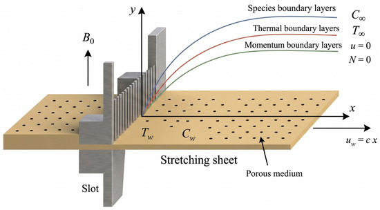
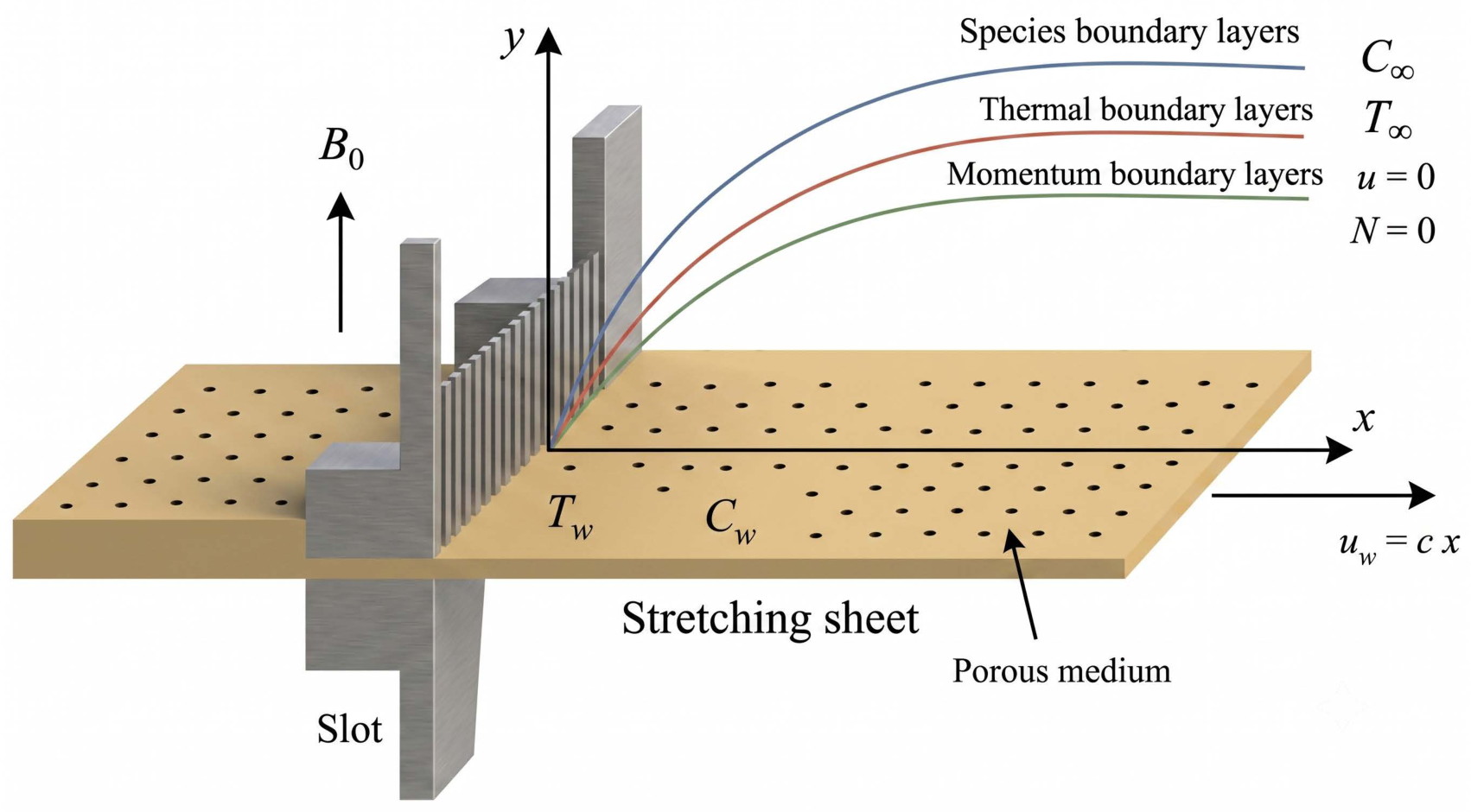
This study presents a mathematical model for a two-dimensional steady flow of a micropolar nanofluid over a stretching surface embedded in a Darcy porous medium. A key feature is the zero nanoparticle mass flux boundary condition, which physically prevents nanoparticle diffusion across the surface under combined Brownian motion and thermophoresis effects, offering a more realistic closure than prescribed concentration. The thermal model incorporates viscous dissipation, Joule heating, thermophoresis, and Brownian motion, while mass transport accounts for chemical reactions and nanoparticle diffusion. The governing conservation laws cover mass, linear and angular momentum, thermal energy, and species concentration, where u and v denote streamwise and transverse velocities, and N represents microrotation. The porous medium resistance is controlled by permeability k, while the transverse magnetic field $B_0$ applied in the y-direction induces electromagnetic damping through electrical conductivity $\sigma$, as shown in Figure 1.

Figure 1. Physical Model and Fluid Transport Description.

The governing equations describing mass, momentum, angular momentum, energy, and species conservation are shaped by several key parameters, the chemical reaction parameter ${{\rm Y}}_1$, ambient concentration $C_{\infty }$ and temperature $T_{\infty }$, thermophoretic diffusion coefficient $D_T$, Brownian diffusion coefficient $D_B$, heat generation factor $Q_0$, thermal conductivity $\kappa$, and specific heat capacity $c_p$. The micropolar nature of the fluid is captured by the vortex viscosity parameter K, where the micro-inertia density is $j=\nu /c$, and the spin-gradient viscosity is defined as $\gamma =\left(\mu +{\displaystyle \frac{K}{2}}\right)j$. Drawing from the described physics, the model equations read [17]:

$${\displaystyle \frac{\partial u}{\partial x}}+{\displaystyle \frac{\partial v}{\partial y}}=0,$$

(1)

$$u{\displaystyle \frac{\partial u}{\partial x}}+v{\displaystyle \frac{\partial u}{\partial y}}=\left({\displaystyle \frac{\mu +K}{\rho }}\right){\displaystyle \frac{{\partial }^{2}u}{\partial y^2}}+{\displaystyle \frac{K}{\rho }}{\displaystyle \frac{\partial N}{\partial y}}-{\displaystyle \frac{1}{\rho }}\left(\sigma B_0^2+{\displaystyle \frac{\mu }{k}}\right)u,$$

(2)

$$\rho j\left(u{\displaystyle \frac{\partial N}{\partial x}}+v{\displaystyle \frac{\partial N}{\partial y}}\right)=\gamma {\displaystyle \frac{{\partial }^{2}N}{\partial y^2}}-\left(K{\displaystyle \frac{\partial u}{\partial y}}+2KN+{\displaystyle \frac{\mu j}{k}}N\right),$$

(3)

$$\begin{array}{cc}\hfill \rho c_p\left(u{\displaystyle \frac{\partial T}{\partial x}}+v{\displaystyle \frac{\partial T}{\partial y}}\right)=& \kappa {\displaystyle \frac{{\partial }^{2}T}{\partial y^2}}+D_B{\displaystyle \frac{\partial C}{\partial y}}{\displaystyle \frac{\partial T}{\partial y}}+{\displaystyle \frac{D_T}{T_{\infty }}}{\left({\displaystyle \frac{\partial T}{\partial y}}\right)}^2+Q_0(T-T_{\infty })\hfill \\ & +{\displaystyle \frac{\partial u}{\partial y}}\left[(\mu +K){\displaystyle \frac{\partial u}{\partial y}}+KN\right]+\sigma B_0^2{u}^2,\hfill \end{array}$$

(4)

$$u{\displaystyle \frac{\partial C}{\partial x}}+v{\displaystyle \frac{\partial C}{\partial y}}=\left(D_B{\displaystyle \frac{{\partial }^{2}C}{\partial y^2}}+{\displaystyle \frac{D_T}{T_{\infty }}}{\displaystyle \frac{{\partial }^{2}T}{\partial y^2}}\right)-{{\rm Y}}_1(C-C_{\infty }).$$

(5)

The governing system (1)–(5) is completed by prescribing [18]:

$$u=cx,{\displaystyle \frac{\partial u}{\partial y}}=-\left({\displaystyle \frac{N}{\omega }}\right)\mathrm{at}y=0,$$

(6)

$$T=T_w,v=\left({\displaystyle \frac{D_B}{C_w-1}}\right){\displaystyle \frac{\partial C}{\partial y}},{\displaystyle \frac{\partial C}{\partial y}}=-\left({\displaystyle \frac{D_T}{D_B{T}_{\infty }}}\right){\displaystyle \frac{\partial T}{\partial y}},\mathrm{at}y=0,$$

(7)

$$(u,N,T,C)\to (0,0,T_{\infty },C_{\infty })\mathrm{as}y\to \infty .$$

(8)

It should be noted that the last term in Equation (7) represents the zero nanoparticle mass flux condition, which implies that no net nanoparticle transport occurs across the wall because the Brownian diffusion and thermophoretic diffusion fluxes exactly balance each other at the boundary. Building on the governing system above, similarity transformations are applied to cast the equations into dimensionless form, yielding [19]:

$$\eta =y\sqrt{{\displaystyle \frac{c}{\nu }}},u=cx{f}^{\prime }\left(\eta \right),v=-\sqrt{c\nu }f\left(\eta \right),$$

(9)

$$\theta ={\displaystyle \frac{T-T_{\infty }}{T_w-T_{\infty }}},\varphi ={\displaystyle \frac{C-C_{\infty }}{C_w-C_{\infty }}},\phi ={\displaystyle \frac{1}{cx}}\sqrt{{\displaystyle \frac{\nu }{c}}}N,$$

(10)

where $\eta$ is the similarity variable, while $\phi$, $\varphi$, and $\theta$ denote dimensionless microrotation, concentration, and temperature, respectively. Substituting (9)–(10) into (1)–(5) automatically satisfies continuity and reduces the system to the following coupled nonlinear ODEs:

$$(1+\Omega )f^{‴}+\Omega {\phi }^{\prime }+f{f}^{″}=f^{\prime }\left(f^{\prime }+M+\chi \right),$$

(11)

$$\left(1+{\displaystyle \frac{\Omega }{2}}\right){\phi }^{″}=(f^{\prime }+\chi +2\Omega )\phi +\Omega f^{″}-f{\phi }^{\prime },$$

(12)

$${\displaystyle \frac{{\theta }^{″}}{Pr}}+f{\theta }^{\prime }+\Gamma \theta +Ec{f}^{″}\left(\Omega f^{″}+\Omega \phi \right)+EcM{f}^{\prime 2}=-\left(G_t{\theta }^{\prime 2}+G_b{\theta }^{\prime }{\varphi }^{\prime }\right),$$

(13)

$${\displaystyle \frac{1}{Le}}{\varphi }^{″}+f{\varphi }^{\prime }={\rm Y}\varphi -{\displaystyle \frac{G_t}{G_b}}{\theta }^{″}.$$

(14)

Equations (11)–(14) are subject to:

$${\varphi }^{\prime }\left(0\right)=-{\displaystyle \frac{G_t}{G_b}}{\theta }^{\prime }\left(0\right),\theta \left(0\right)=1,f^{\prime }\left(0\right)=1,\phi \left(0\right)=-\omega f^{″}\left(0\right),f\left(0\right)={\displaystyle \frac{\delta }{Le}}{\varphi }^{\prime }\left(0\right),$$

(15)

$$\left(f^{\prime },\theta ,\varphi ,\phi \right)\to \left(0,0,0,0\right)\mathrm{as}\eta \to \infty .$$

(16)

These transformed governing equations constitute a strongly coupled and highly nonlinear system of ordinary differential equations. Owing to the complex interactions among the nonlinear terms, variable thermophysical properties, and boundary conditions, obtaining a closed-form analytical solution is generally infeasible. Consequently, an accurate numerical framework is required to determine the solution. In the present study, a Physics-Informed Neural Network (PINN) is employed as the computational solver. Unlike conventional numerical techniques, the PINN incorporates the governing physical laws directly into the training process by minimizing the residuals of the differential equations while simultaneously enforcing the prescribed boundary conditions. The model is characterized by the following eleven dimensionless groups:

$$\left\{\begin{array}{cc}Pr={\displaystyle \frac{\mu c_p}{\kappa }}\hfill & \mathrm{Prandtl}\mathrm{number},\hfill \\ M={\displaystyle \frac{\sigma B_0^2}{\rho c}}\hfill & \mathrm{Magnetic}\mathrm{number},\hfill \\ Le={\displaystyle \frac{\nu }{D_B}}\hfill & \mathrm{Lewis}\mathrm{number},\hfill \\ Ec={\displaystyle \frac{u_w^2}{c_p(T_w-T_{\infty })}}\hfill & \mathrm{Eckert}\mathrm{number},\hfill \\ \chi ={\displaystyle \frac{\nu }{ck}}\hfill & \mathrm{Porous}\mathrm{factor},\hfill \\ \delta ={\displaystyle \frac{C_w-C_{\infty }}{1-C_w}}\hfill & \mathrm{Stefan}\mathrm{blowing},\hfill \\ G_b={\displaystyle \frac{D_B(C_w-C_{\infty })}{\mu c_p}}\hfill & \mathrm{Brownian}\mathrm{motion}\mathrm{factor},\hfill \\ G_t={\displaystyle \frac{D_T(T_w-T_{\infty })}{\mu c_p{T}_{\infty }}}\hfill & \mathrm{Thermophoresis}\mathrm{factor},\hfill \\ {\rm Y}={\displaystyle \frac{{{\rm Y}}_1}{c}}\hfill & \mathrm{Chemical}\mathrm{reaction}\mathrm{factor},\hfill \\ \Omega ={\displaystyle \frac{K}{\mu }}\hfill & \mathrm{Vortex}\mathrm{viscosity}\mathrm{coefficient},\hfill \\ \Gamma ={\displaystyle \frac{Q_0}{\rho c_{p}c}}\hfill & \mathrm{Heat}\mathrm{generation}/\mathrm{absorption}\mathrm{factor}.\hfill \end{array}\right.$$

Four engineering quantities of practical interest are examined, the skin-friction coefficient $C{f}_x$, wall couple stress $M_x$, Sherwood number $S{h}_x$, and Nusselt number $N{u}_x$, expressed as:

$$C{f}_{x}R{e}^{{\displaystyle \frac{1}{2}}}=-\Omega \left(\phi +f^{″}\right),S{h}_{x}R{e}^{-{\displaystyle \frac{1}{2}}}=-{\varphi }^{\prime }\left(0\right),$$

(17)

measuring the surface drag due to viscous resistance and reflecting the wall mass flux of nanoparticles; respectively. Further, both the following equations

$$M_{x}Re=-\left(1+{\displaystyle \frac{\Omega }{2}}\right){\phi }^{\prime }\left(0\right),N{u}_{x}R{e}^{-{\displaystyle \frac{1}{2}}}=-{\theta }^{\prime }\left(0\right),$$

(18)

capturing micro-scale rotational effects at the surface and quantifying the convective heat transfer rate.

3. PINN Solution

Firstly, we must mention here that the proposed PINN is employed to solve the transformed system of ordinary differential Equations (11)–(14) subject to the prescribed boundary conditions (15)–(16). Unlike conventional data-driven neural networks, the proposed PINN is fundamentally grounded in physical laws, with the governing equations and boundary conditions explicitly enforced during the training process. The PINN is designed to serve as a single, continuous surrogate that captures the behavior of a tightly coupled, nonlinear ODE system across an 8-dimensional parameter space eliminating the need to re-solve the governing equations each time a parameter change. The network takes as input the dimensionless coordinate $\eta$ alongside seven physical parameters, and produces four solution profiles as output. Formally, the input and output vectors are defined as:

$${\mathbf{h}}^{\left(1\right)}={\sigma }_1\left({\mathbf{W}}^{\left(1\right)}\mathbf{x}+{\mathbf{b}}^{\left(1\right)}\right).$$

(19)

For the subsequent hidden layers ($l=2,\dots ,L$), the input injection is applied via vector concatenation:

$${\mathbf{h}}^{\left(l\right)}={\sigma }_1\left({\mathbf{W}}^{\left(l\right)}\left[{\mathbf{h}}^{(l-1)},\mathbf{x}\right]+{\mathbf{b}}^{\left(l\right)}\right).$$

(20)

The final predicted physical fields are generated through a linear output layer $(L+1)$:

$$\widehat{\mathbf{u}}={\mathbf{W}}^{(L+1)}{\mathbf{h}}^{\left(L\right)}+{\mathbf{b}}^{(L+1)},$$

(21)

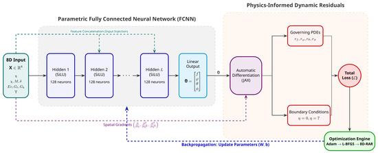
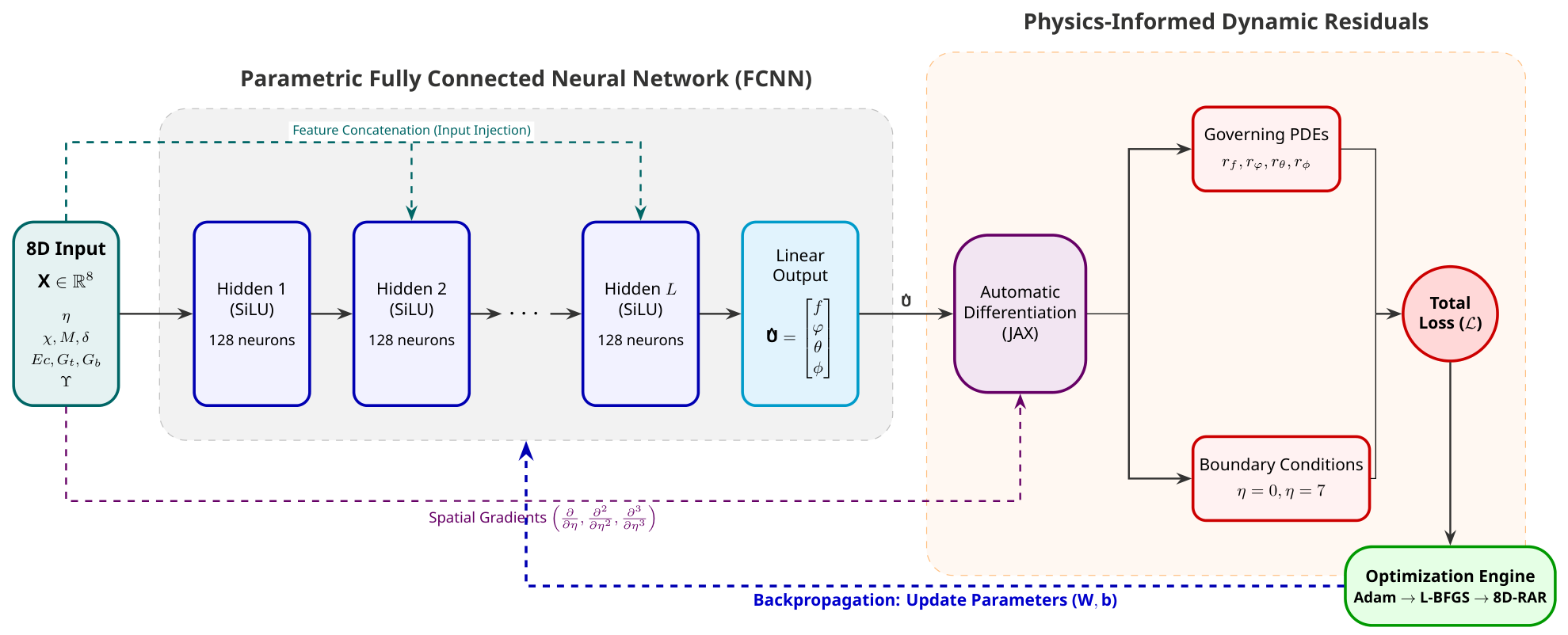
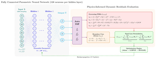
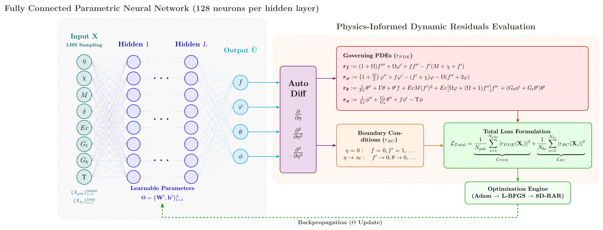
where ${\mathbf{W}}^{\left(l\right)}$ and ${\mathbf{b}}^{\left(l\right)}$ represent the learnable weight matrices and bias vectors of the l-th layer, respectively, and $[·,·]$ denotes the concatenation operation. The PINN consists of hidden layers with 128 neurons each, initialized via He-Normal scaling to ensure stable early training [20]. To preserve numerical integrity throughout the high-dimensional optimization process, all network computations and automatic differentiation operations are enforced in 64-bit floating-point precision (Float64), guarding against underflow and ensuring accuracy in higher-order derivative evaluations, which are particularly susceptible to truncation errors. The complete architecture encompassing input injection, automatic differentiation, and physics-based loss construction is illustrated in Figure 2. As shown, spatial gradients extracted from the network output are directly channeled into the physics-informed residual block, ensuring that the underlying governing equations actively constrain the learning process during backpropagation. Here, we must mention that we employ the Sigmoid Linear Unit (SiLU) across all PINN hidden layers to ensure surrogate model differentiability. SiLU’s smooth and infinitely differentiable ($C^{\infty }$) properties are essential for computing the required third-order spatial derivatives via automatic differentiation, avoiding the zero-gradient issues associated with non-smooth functions.

Figure 2. Schematic representation of the proposed Parametric Physics-Informed Neural Network (PINN) framework.

3.1. Physics-Based Dynamic Loss Construction

As shown in Figure 3, the PINN’s core learning mechanism relies on a residual-based loss that enforces physical consistency. Rather than learning from labeled data, the network operates unsupervised, penalizing any deviation from the governing equations and boundary conditions. Spatial derivatives of the predicted fields with respect to the dimensionless coordinate $\eta$ are computed via forward-mode Automatic Differentiation, a deliberate choice over finite difference schemes, which introduce truncation errors [21]. Since all required gradients involve a single independent variable, $\eta$, forward-mode AD is computationally optimal in the present framework. Within JAX, the chain rule is applied at the compiler level, yielding machine-precision derivatives. Using these exact derivatives, the governing nonlinear ODEs are reformulated as residual functions [22]. It is worth noting that the governing parameters are fixed thermophysical constants associated with the fluid model and remain unchanged throughout the parametric domain. Let ${\eta }_i$ denote the i-th collocation point. The residuals corresponding to the momentum ($r_f$), microrotation ($r_{\phi }$), energy ($r_{\theta }$), and concentration ($r_{\varphi }$) equations are defined as follows:

$$r_f=(1+\Omega )f^{‴}+\Omega {\phi }^{\prime }+f{f}^{″}-f^{\prime }(M+\chi +f^{\prime }),$$

(22)

$$r_{\phi }=\left(1+{\displaystyle \frac{\Omega }{2}}\right){\phi }^{″}+f{\phi }^{\prime }-(f^{\prime }+\chi )\phi -\Omega (f^{″}+2\phi ),$$

(23)

$$r_{\theta }={\displaystyle \frac{1}{\mathrm{Pr}}}{\theta }^{″}+\Gamma \theta +{\theta }^{\prime }f+EcM{\left(f^{\prime }\right)}^2+Ec(\Omega \phi +\Omega f^{″})f^{″}+(G_b{\varphi }^{\prime }+G_t{\theta }^{\prime }){\theta }^{\prime },$$

(24)

$$r_{\varphi }={\displaystyle \frac{1}{Le}}{\varphi }^{″}+{\displaystyle \frac{G_t}{G_b}}{\theta }^{″}+f{\varphi }^{\prime }-{\rm Y}\varphi .$$

(25)

Beyond the interior physics, the MLP is further constrained by wall $\eta =0$ and far-field ($\eta \to \infty$) boundary conditions. In practice, the far-field is truncated at a finite boundary ${\eta }_{\infty }=7.0$ large enough to capture the asymptotic decay accurately. The corresponding boundary residual vectors are given by:

$${\mathbf{r}}_{bco}:=\left[f^{\prime }\left(0\right)-1,f\left(0\right)-{\displaystyle \frac{\delta }{Le}}{\varphi }^{\prime }\left(0\right),\phi \left(0\right)+\omega f^{″}\left(0\right),{\varphi }^{\prime }\left(0\right)+{\displaystyle \frac{G_t}{G_b}}{\theta }^{\prime }\left(0\right),\theta \left(0\right)-1\right]\mathrm{at}\eta =0,$$

(26)

$${\mathbf{r}}_{bc\infty }:=\left[f^{\prime },\phi ,\theta ,\varphi \right]\mathrm{at}\eta ={\eta }_{\infty }.$$

(27)

The overall optimization objective is to find the optimal set of network parameters ${\theta }^{\ast }$ that minimizes the total composite loss function ${\mathcal{L}}_{Total}$. This formulation aggregates the Mean Squared Error (MSE) of the physics residuals (${\mathcal{L}}_{PDE}$) and the boundary condition residuals (${\mathcal{L}}_{BC}$):

$${\mathcal{L}}_{Total}={\mathcal{L}}_{PDE}+{\mathcal{L}}_{BC},$$

(28)

$${\mathcal{L}}_{PDE}={\displaystyle \frac{1}{N_{pde}}}{\displaystyle \sum _{i=1}^{N_{pde}}}\left({\left|r_f\left({\mathbf{x}}_i\right)\right|}^2+{\left|r_{\phi }\left({\mathbf{x}}_i\right)\right|}^2+{\left|r_{\theta }\left({\mathbf{x}}_i\right)\right|}^2+{\left|r_{\varphi }\left({\mathbf{x}}_i\right)\right|}^2\right),$$

(29)

$${\mathcal{L}}_{BC}={\displaystyle \frac{1}{N_{bc}}}{\displaystyle \sum _{j=1}^{N_{bc}}}\left({∥{\mathbf{r}}_{bc0}\left({\mathbf{x}}_j\right)∥}_2^2+{∥{\mathbf{r}}_{bc\infty }\left({\mathbf{x}}_j\right)∥}_2^2\right),$$

(30)

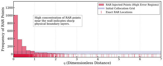
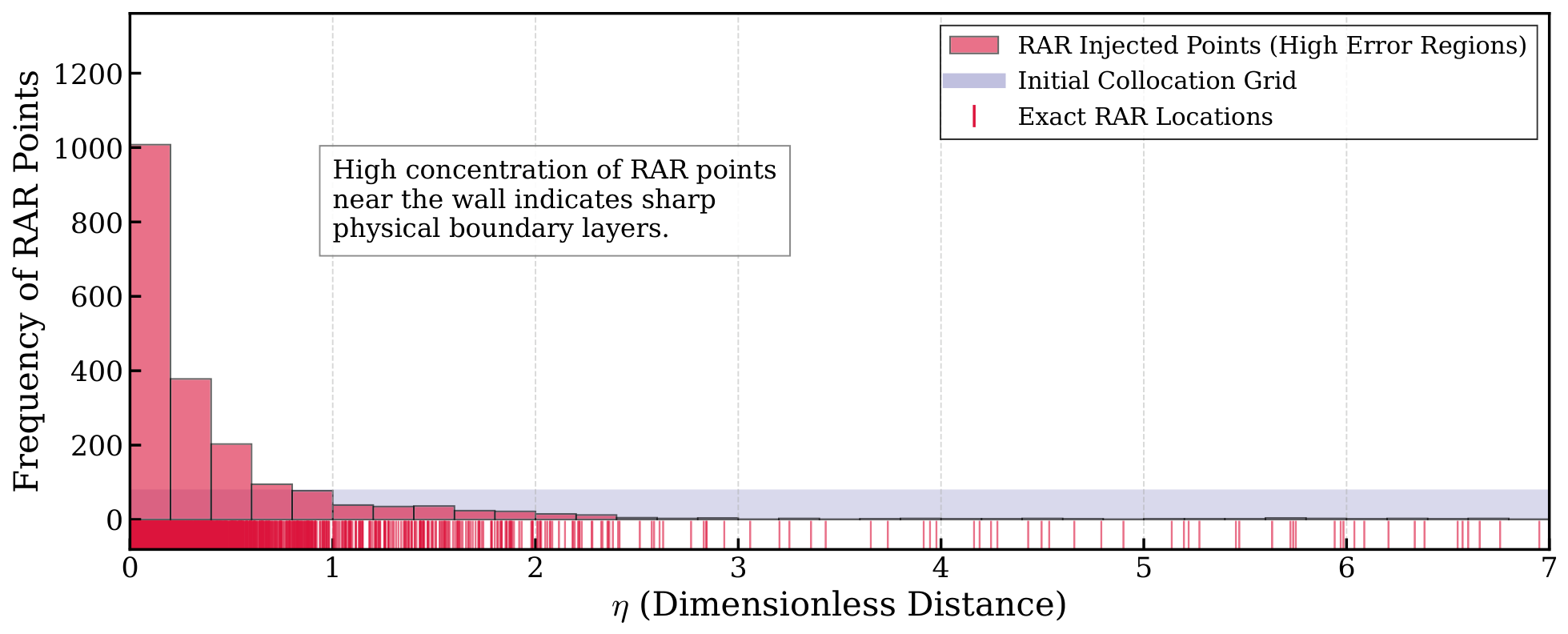
where ${\mathbf{x}}_i$∈${\mathbb{R}}^8$, $N_{pde}$ and $N_{bc}$ are the total number of parametric collocation points sampled inside the domain and at the boundaries, respectively. Additionally, training the PINN over a high-dimensional parametric space is addressed using Latin Hypercube Sampling (LHS), which ensures uniform, space-filling coverage of the domain. The initial dataset comprises interior and boundary collocation points at both the wall and far-field. To further resolve sharp near-wall gradients inherent to stretching sheet flows, a one-shot Residual-based Adaptive Refinement (RAR) strategy is applied following an initial hybrid optimization phase [23]. New candidate points are drawn across the full parameter space, and since the optimizer has already reduced the global loss substantially, a single refinement step is sufficient to capture the remaining boundary layer features without iterative resampling. The spatial distribution of these added points is shown in the following Figure 4.

Figure 3. Detailed schematic of the physics-informed residual evaluation within the PINN framework.

Figure 4. Spatial distribution histogram of the collocation points appended by the 8D-RAR algorithm.

3.2. Hybrid Optimization and Convergence Analysis

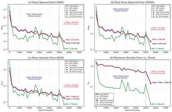
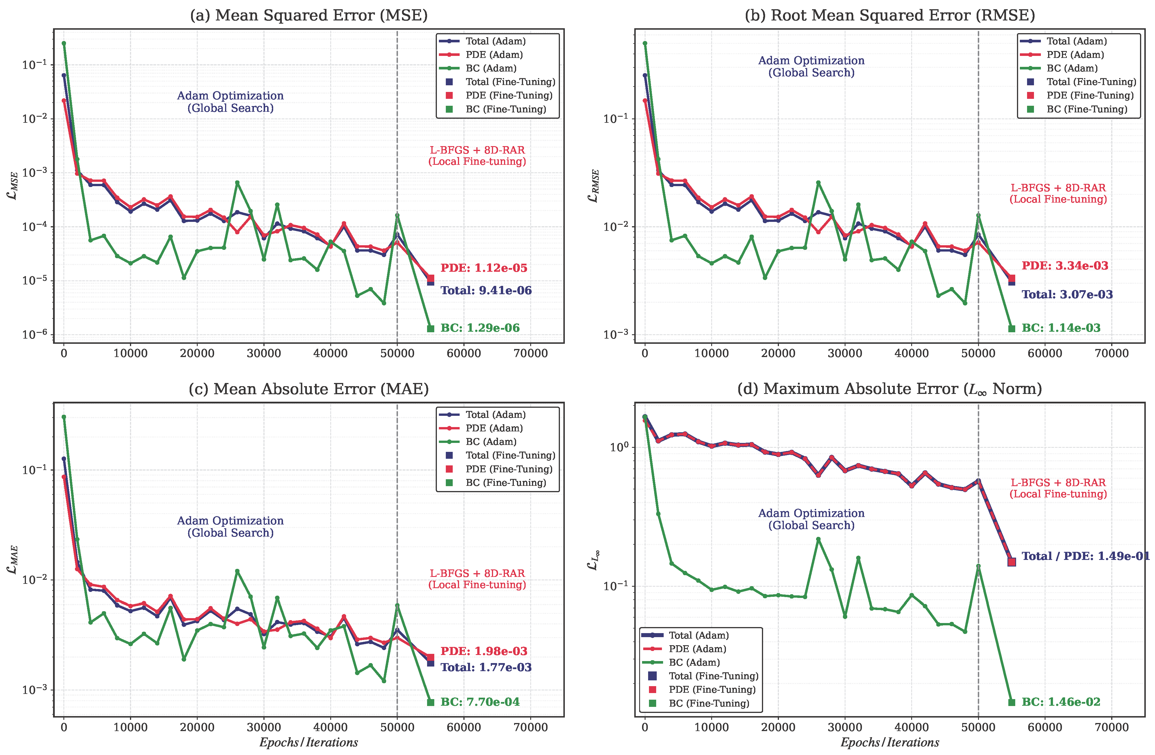
This section evaluates the predictive performance and accuracy of the proposed framework through a comprehensive error analysis based on several standard statistical metrics. Therefore, Figure 5a–d present the error assessment of the proposed model using four widely adopted statistical indicators: Mean Squared Error (MSE), Root Mean Squared Error (RMSE), Mean Absolute Error (MAE), and Maximum Absolute Error ($L_{\infty }$ norm). Figure 5a illustrates the variation of MSE, reflecting the average squared deviation between the predicted and reference solutions. Figure 5b depicts the RMSE values, providing an error measure in the same units as the target variable and offering a more intuitive interpretation of prediction accuracy. Figure 5c shows the MAE distribution, which quantifies the average magnitude of absolute deviations without emphasizing large errors. Finally, Figure 5d presents the maximum absolute error ($L_{\infty }$ norm), highlighting the worst-case discrepancy observed across the computational domain. Collectively, these metrics demonstrate the predictive reliability and numerical robustness of the proposed framework.

Figure 5. Convergence histories of the comprehensive error metrics during the hybrid optimization process across the 8D parametric space: (a) Mean Squared Error (MSE), (b) Root Mean Squared Error (RMSE), (c) Mean Absolute Error (MAE), and (d) Maximum Absolute Error.

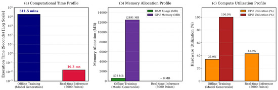
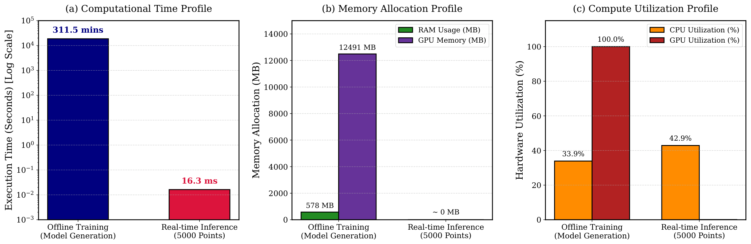
Finally, Figure 6a–c compare the computational requirements of the proposed framework during the offline training stage and the real-time inference stage. Figure 6a presents the execution time on a logarithmic scale, highlighting the substantial reduction in computational cost achieved during inference. Figure 6b illustrates the corresponding GPU and RAM allocations, providing insight into memory consumption across both phases. Figure 6c shows the hardware utilization percentages, reflecting the efficiency of resource usage during model generation and deployment. Overall, the results demonstrate that the computationally intensive offline training process enables highly efficient real-time predictions with minimal resource demands.

Figure 6. Computational resource profiling of the PINN framework. The bar charts contrast offline model generation against real-time inference across: (a) execution time, (b) GPU/RAM consumption, and (c) Hardware utilization.

4. Physics-Informed Neural Network Validation

The correctness of the developed Physics-Informed Neural Network (PINN) technique is verified through Table 1, which provides a comparison of the wall shear coefficient, $-f^{″}\left(0\right)$, and the corresponding values obtained by the finite-element method that presented previously by Kumar [24]. A good correspondence is achieved over the whole domain of the vortex viscosity parameter $\Omega$, showing the validity of the developed computational scheme. The differences between the datasets under consideration are very low, the maximum relative deviation reaching $0.0038\%$ at $\Omega =0.5$ and the minimum relative error being about $0.00004\%$ at $\Omega =0.0$.

Table 1. $-f^{″}\left(0\right)$ values in changing $\Omega$ with $\omega =M=0.5,$ $\delta =0.0$ and $\chi =0.0$.

$\mathbf{\Omega }$	Kumar ([24])	Present Work
0.0	1.1890	1.18899952147
0.5	1.0590	1.05895978902
1.0	0.9676	0.96757975839
2.0	0.8424	0.84238819547

5. Numerical Results and Discussion

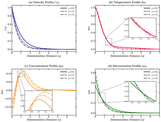
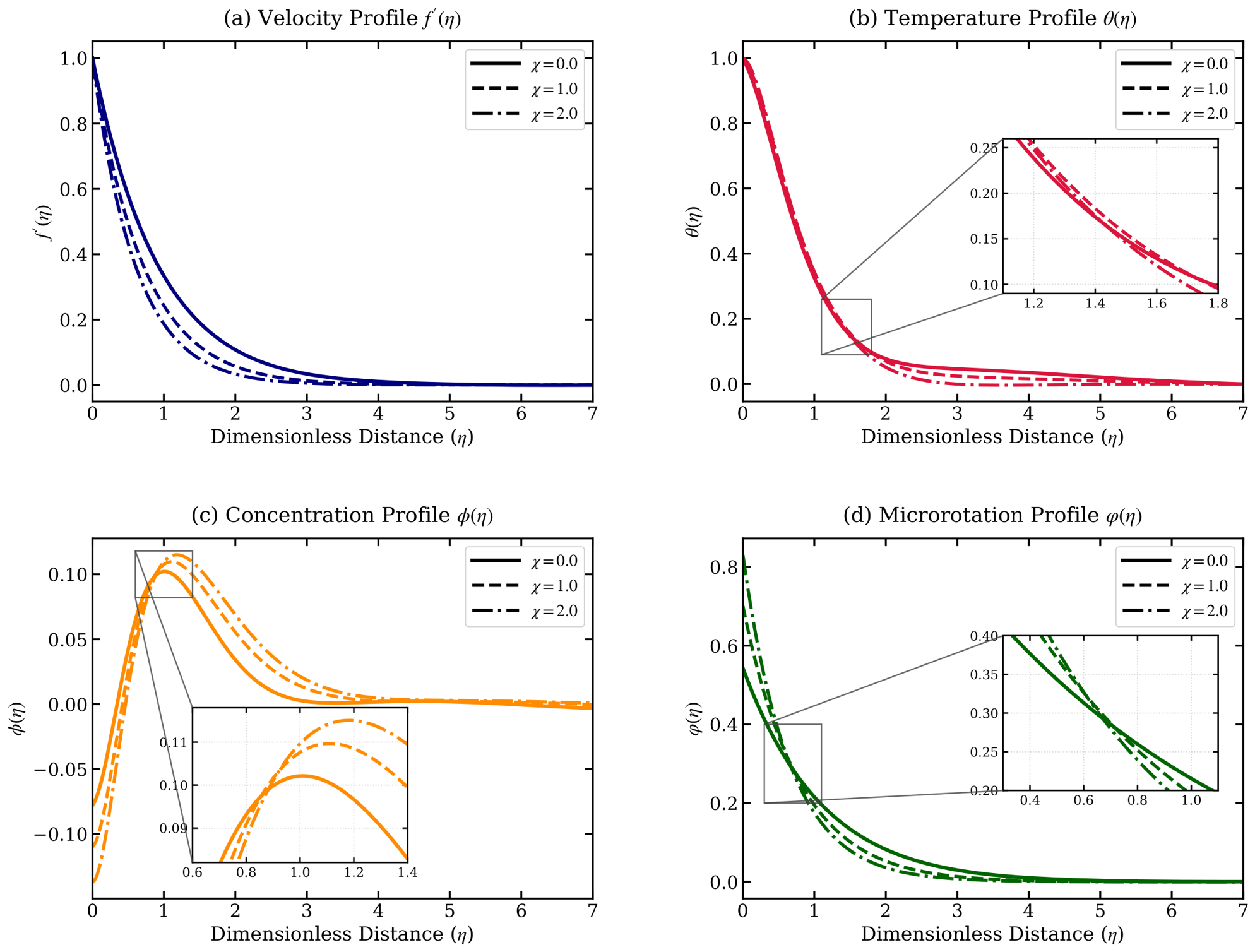
This section presents a comprehensive numerical investigation of the proposed mathematical model using the Physics-Informed Neural Network (PINN) solution. The obtained results are analyzed to illustrate the influence of the governing physical parameters on the flow, thermal, microrotation and concentration characteristics of the system. Particular attention is given to the accuracy, stability, and predictive capability of the PINN framework in capturing the underlying physical behavior. The numerical findings provide valuable insights into the complex interactions among the model parameters and demonstrate the effectiveness of the proposed approach in solving the governing nonlinear equations. Figure 7 comprehensively illustrates the response of the dimensionless velocity $f^{\prime }\left(\eta \right)$, temperature $\theta \left(\eta \right)$, concentration $\varphi \left(\eta \right)$, and microrotation $\phi \left(\eta \right)$ profiles to variations in the porous factor $\chi$. As depicted in Figure 7a,d, an increment in $\chi$ induces a profound deceleration in both the primary fluid velocity $f^{\prime }\left(\eta \right)$ and the microrotation $\phi \left(\eta \right)$. It is worth noting that the microrotation profile exhibits a similar trend to the velocity profile far from the stretching sheet; however, in the vicinity of the sheet, this behavior is reversed. Physically, increasing $\chi$ reduces the medium’s permeability, strengthening the Darcy resistive drag that opposes the flow. This resistance hinders fluid motion near the stretching sheet, leading to a thinner hydrodynamic boundary layer. Consequently, the weakened velocity field suppresses the micro-rotational momentum of the suspended particles, causing the angular velocity to decay more rapidly. Further, the corresponding thermodynamic and concentration boundary layer responses are portrayed in Figure 7b,c. The influence of the porous parameter $\chi$ on the thermal profile $\theta \left(\eta \right)$ reveals a notable spatial contrast that deserves careful attention. In the immediate vicinity of the stretching sheet, increasing $\chi$ produces a marginal rise in fluid temperature, whereas far from the sheet, the opposite trend emerges with considerably greater intensity. Physically, near the sheet surface, the increased flow resistance induced by higher permeability reduction traps thermal energy within the fluid, causing a slight local temperature elevation. However, as the distance from the sheet grows, the severely attenuated velocity field weakens convective heat transport away from the surface, allowing the thermal boundary layer to thin more rapidly in the outer region, which ultimately drives the temperature down at locations far from the sheet. Also, a particularly noteworthy feature arises from the imposition of the zero nanoparticle mass flux condition at the sheet surface, which drives the concentration profile $\varphi \left(\eta \right)$ into negative territory in the near-wall region. In this zone, increasing $\chi$ further suppresses the concentration values. Far from the sheet, however, the trend reverses, and the concentration rises noticeably with growing $\chi$. Physically, the zero mass flux condition drives nanoparticles away from the surface, creating a concentration deficit near the wall. The porous medium further enhances this depletion by restricting particle transport toward the sheet, whereas the slower flow in the outer region increases particle residence time, leading to a gradual concentration accumulation away from the surface.

Figure 7. Influence of the porous factor $\chi$ on (a) the velocity $f^{\prime }\left(\eta \right)$, (b) the temperature $\theta \left(\eta \right)$, (c) the concentration $\varphi \left(\eta \right)$, and (d) the microrotation $\phi \left(\eta \right)$ profiles.

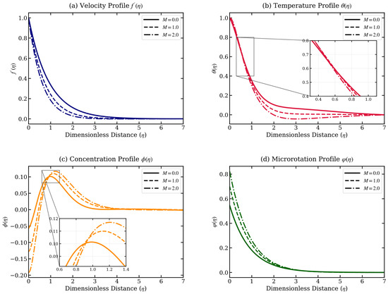
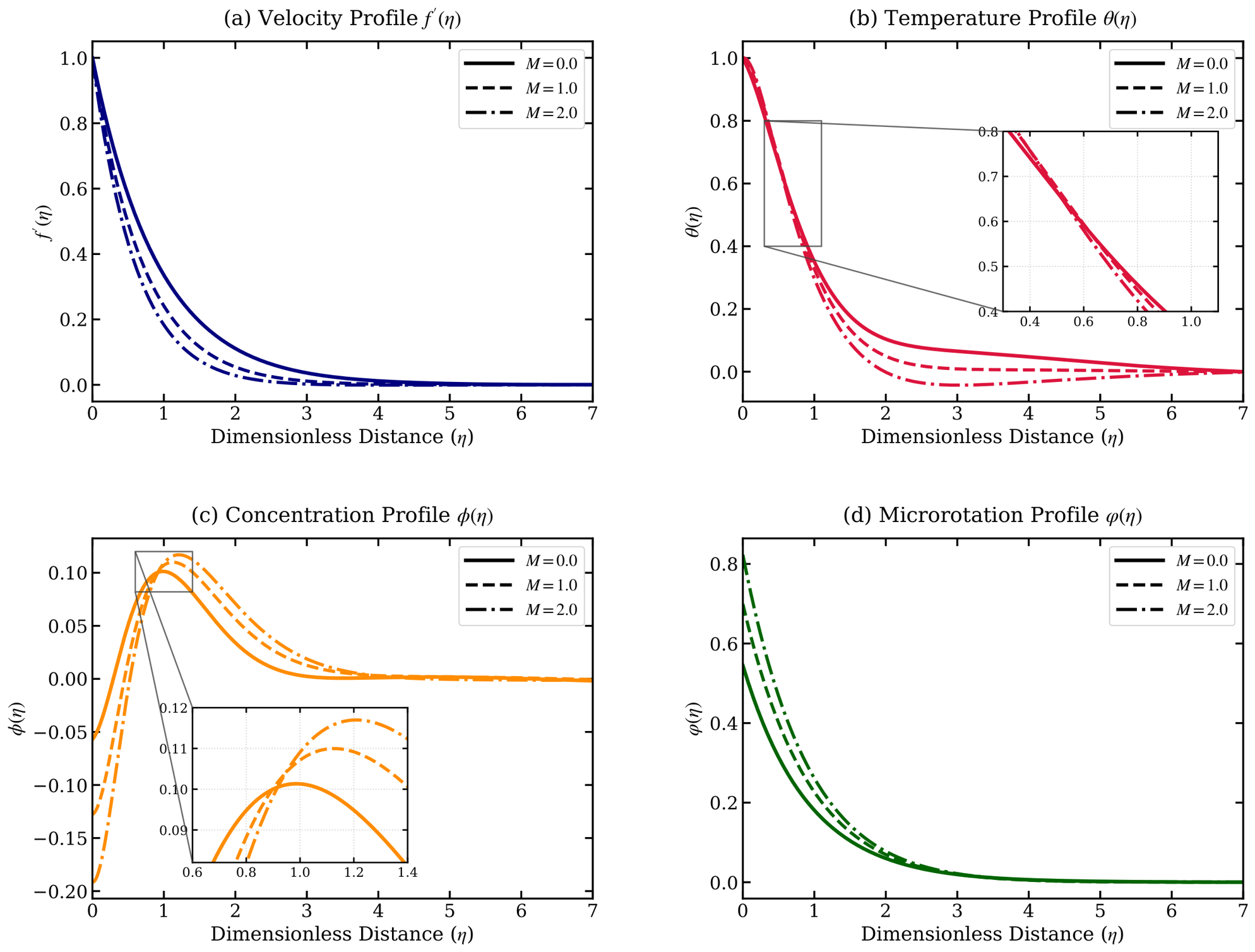
Figure 8 comprehensively delineates the physical impact of the magnetic parameter M on the fundamental boundary layer profiles $f^{\prime }\left(\eta \right)$, $\varphi \left(\eta \right)$, $\theta \left(\eta \right)$ and $\phi \left(\eta \right)$. As shown in Figure 8a, strengthening the magnetic field progressively decelerates the fluid velocity $f^{\prime }\left(\eta \right)$, owing to the retarding Lorentz force that acts perpendicular to the flow direction. Interestingly, the microrotation profile $\phi \left(\eta \right)$ responds in the opposite manner, exhibiting a clear enhancement with rising M, since the suppressed translational motion redirects rotational momentum toward the suspended micro-elements. Regarding the thermal response in Figure 8b, the magnetic parameter produces a slight temperature rise near the stretching sheet, where Joule dissipation locally accumulates thermal energy, while far from the surface the temperature drops markedly as the weakened convective transport fails to sustain the thermal boundary layer in the outer region. A particularly interesting behavior emerges in the concentration field $\varphi \left(\eta \right)$, as shown in Figure 8c, under the zero nanoparticle mass flux condition. Near the sheet, where concentration values already begin in the negative range, increasing M further deepens this deficit by restricting particle replenishment through the attenuated flow. Away from the surface, however, the trend reverses noticeably, as the decelerated outer flow extends particle residence time, leading to a measurable concentration buildup in that region.

Figure 8. Influence of the magnetic parameter M on (a) the velocity $f^{\prime }\left(\eta \right)$, (b) the temperature $\theta \left(\eta \right)$, (c) the concentration $\varphi \left(\eta \right)$, and (d) the microrotation $\phi \left(\eta \right)$ profiles.

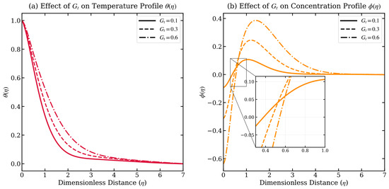
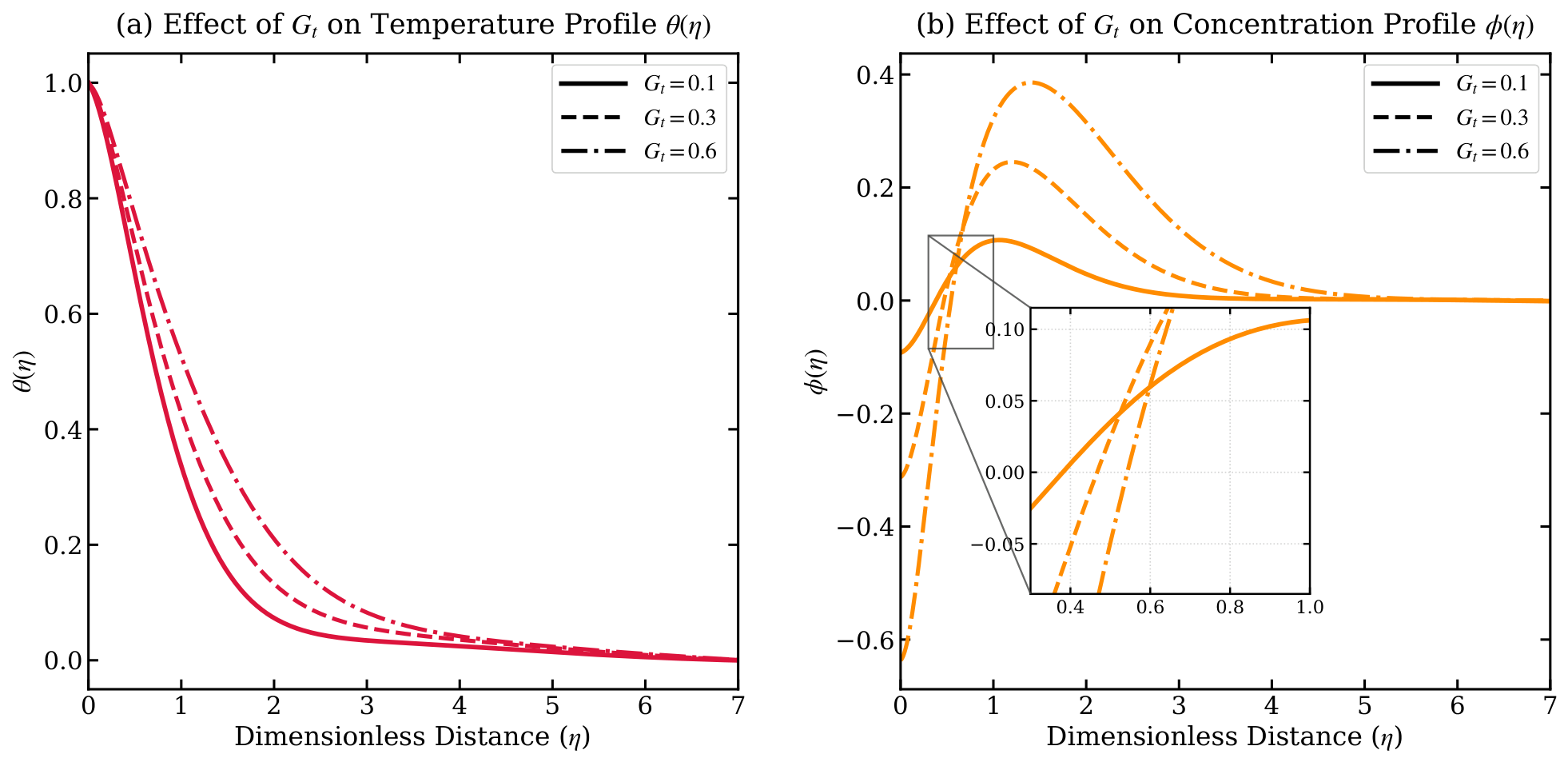
The inclusion of nanoscale effects, specifically thermophoresis phenomenon though the factor $D_t$, critically governs the coupled heat and mass transfer characteristics within nanofluids. Therefore, the distinct physical implications of this mechanism are systematically isolated and evaluated in Figure 9. Clearly that the thermophoresis parameter plays a significant role in governing both the thermal and concentration fields across the boundary layer. As $D_t$ increases, the temperature distribution is enhanced throughout the entire boundary layer thickness, which is physically attributed to the thermophoretic force that drives nanoparticles from hot regions near the sheet toward cooler regions away from it, thereby intensifying heat transfer and elevating the thermal boundary layer. The influence of $D_t$ on the concentration profile, however, exhibits a more intriguing and non-uniform behavior. Far from the sheet, the concentration distribution follows a trend analogous to that of the temperature, increasing with rising values of $D_t$ since the thermophoretic migration of nanoparticles accumulates them in the outer region of the boundary layer. In contrast, in the vicinity of the sheet surface, the effect is completely reversed; the concentration values are observed to decrease and notably begin with negative magnitudes near the wall. This seemingly counterintuitive behavior is a direct consequence of the zero nanoparticle mass flux condition imposed at the plate surface, which physically means that no nanoparticles are allowed to penetrate or accumulate at the wall. Under this condition, the thermophoretic flux pushing particles away from the hot wall must be exactly balanced by the Brownian diffusion flux directed toward the wall, resulting in a reduced and even negative nanoparticle concentration gradient near the surface.

Figure 9. Influence of the thermophoresis parameter $D_t$ on (a) the temperature $\theta \left(\eta \right)$, and (b) concentration $\varphi \left(\eta \right)$ profiles.

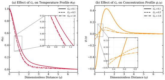
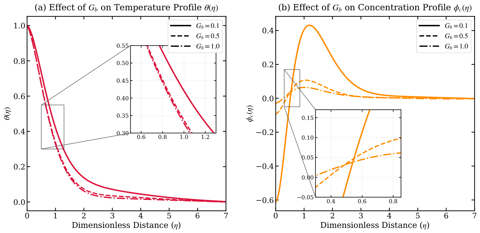
Figure 10 is dedicated to isolating and examining the sole physical contribution of Brownian motion, characterized by the parameter $D_b$, to the intertwined heat and mass transfer behavior inherent to nanofluid systems. Elevating $D_b$ progressively attenuates the thermal boundary layer, as more vigorous random particle motion redistributes thermal energy more uniformly, eroding the temperature gradient. The concentration field, however, responds in a spatially split manner, far from the plate, broader nanoparticle dispersal mirrors the thermal suppression, while near the wall the trend inverts sharply concentration rises with $D_b$ yet departs from negative wall values. This sign reversal is a direct fingerprint of the zero nanoparticle mass flux condition, which compels Brownian diffusion and thermophoretic flux into exact mutual cancellation at the surface, leaving the immediate wall region depleted of nanoparticles.

Figure 10. Influence of the Brownian motion parameter $D_b$ on (a) the temperature $\theta \left(\eta \right)$, and (b) concentration $\varphi \left(\eta \right)$ profiles.

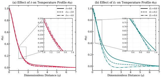
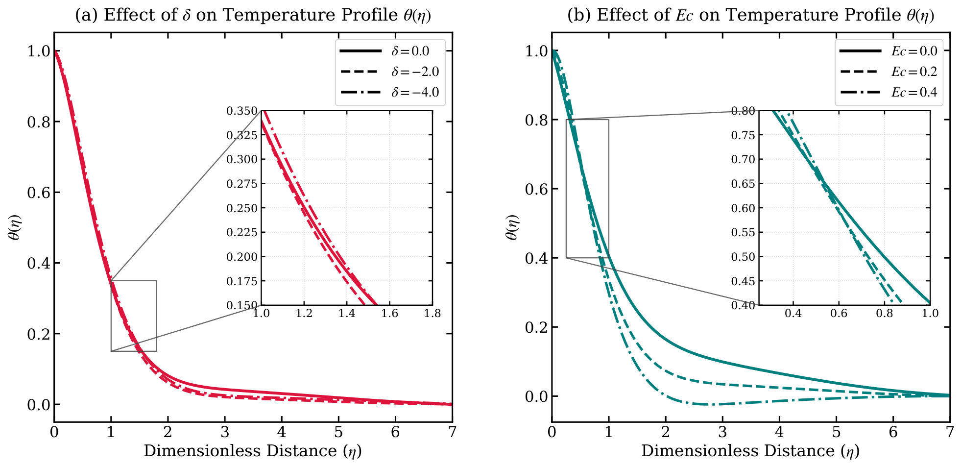
Figure 11 isolates and contrasts the effects of the Stefan blowing parameter $\delta$ and the Eckert number $Ec$ on the dimensionless temperature profile $\theta \left(\eta \right)$. Strengthening the Stefan blowing magnitude acts as a thermal suppressant, with its cooling footprint becoming increasingly pronounced away from the stretching sheet, as the outward mass injection drives a convective sweep that expels heat from the wall and starves the far-field region of thermal energy. The Eckert number, by contrast, imprints a spatially split thermal signature, where near the wall, viscous dissipation converts mechanical energy into heat, nudging the temperature modestly upward, yet this wall-anchored mechanism loses its grip with distance, and in the outer layer, stronger fluid inertia takes over as an effective coolant, producing a dramatic temperature drop that completely overshadows the near-wall warming trend.

Figure 11. Thermodynamic response of the temperature profile $\theta \left(\eta \right)$ to variations in (a) the thermal stratification parameter $\delta$ and (b) the Eckert number $Ec$.

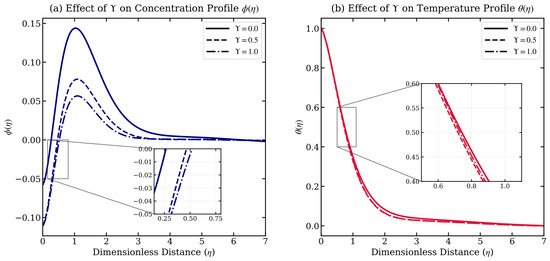
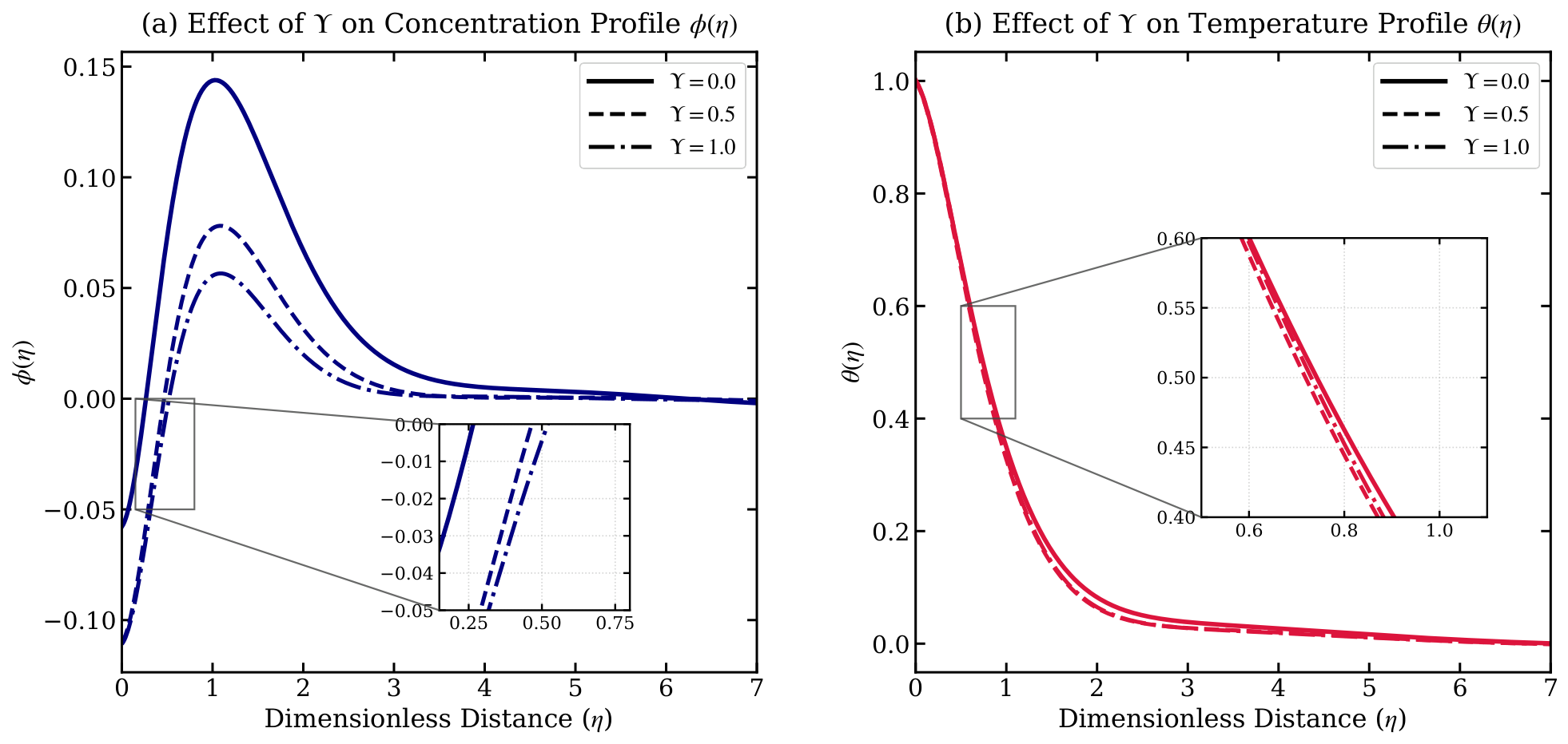
Figure 12 comprehensively delineates the physical impact of the chemical reaction parameter ${\rm Y}$ on both the concentration $\varphi \left(\eta \right)$ and thermal $\theta \left(\eta \right)$ fields. The chemical reaction parameter ${\rm Y}$ exerts a dominant and highly pronounced suppressive effect on the concentration field throughout the boundary layer. This strong attenuation is physically direct and expected, since this parameter appears explicitly in the concentration governing equation, where a destructive chemical reaction continuously consumes nanoparticles as reactants, depleting their local concentration and steepening the concentration gradient toward the wall. The thermal field, however, is not entirely immune to this parameter’s influence. A mild yet discernible reduction in temperature distribution is also observed with increasing ${\rm Y}$, albeit of considerably smaller magnitude compared to the dramatic concentration suppression. This subtle thermal damping is physically indirect, as the chemical reaction depletes the nanoparticle concentration, the capacity of the nanofluid to carry and retain thermal energy is marginally weakened, leading to a modest but measurable cooling effect on the temperature profile across the boundary layer.

Figure 12. Influence of the chemical reaction parameter ${\rm Y}$ on (a) the concentration $\varphi \left(\eta \right)$, and (b) the temperature $\theta \left(\eta \right)$ profiles.

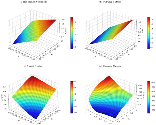
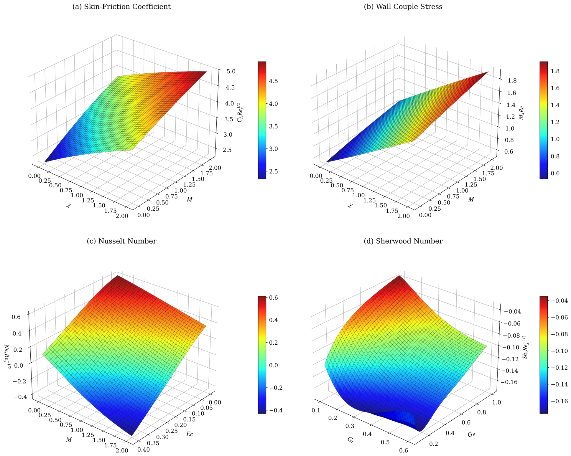
As shown in Figure 13a, both the porous factor $\chi$ and the magnetic parameter M show an increasing influence on the skin friction coefficient. The physical reasoning behind this observation is the fact that an increase in the porous parameter increases the drag force exerted on the fluid by the porous medium, whereas an increase in the magnetic parameter creates a drag force due to the Lorentz force created against the fluid flow. As such, these two parameters increase the drag force experienced by the fluid flow. In Figure 13b, we notice that the same two parameters have an increasing effect on the wall couple stress as well; but compared with the skin friction coefficient, the increment is quite small. The reason for this can be attributed to the fact that wall couple stress is dependent on the microrotation of the fluid, which is not as strongly influenced by magnetic and porous drag forces compared with the translational velocity field. It can be seen clearly from Figure 13c that both the magnetic field parameter and the Eckert number play an important role in the reduction of the Nusselt number. The reasons for such behavior are physical and may be explained by the following considerations. On the one hand, with the increase of the magnetic field parameter, the presence of the Lorentz force caused by the applied magnetic field opposes the flow of the fluid and results in the additional Ohmic dissipation of the fluid, and consequently, in its heating. As the result, the thermal gradient between the wall and the surrounding fluid becomes smaller, and the rate of heat exchange decreases causing the Nusselt number to become smaller as well. On the other hand, the larger value of the Eckert number means a more important role of viscous dissipation phenomena in the conversion of the mechanical energy to thermal one. This phenomenon of heating of the fluid again leads to a decrease of the thermal gradient near the wall surface and results in the reduction of the convective heat exchange and the decrease of the Nusselt number. Further, as illustrated in Figure 13d below, the thermophoresis and Brownian motion coefficients have contrasting influences on the local Sherwood number. The higher values of the thermophoresis coefficient cause gradual increase in the value of the Sherwood number because thermophoresis causes the nanoparticles to move from the wall towards the cold surface, hence reducing the concentration gradient and mass transfer process. On the other hand, an increase in the value of the Brownian motion coefficient results in the enhancement of the value of the Sherwood number due to increased diffusion process.

Figure 13. Impact of $\chi$ and M on (a) skin friction and (b) wall couple stress, M and $Ec$ on (c) Nusselt number, and $G_b$ and $G_t$ on (d) Sherwood number.

6. Concluding Remarks

This study demonstrates the effectiveness of physics-informed neural networks in solving the proposed physical model. The obtained results exhibit good agreement with benchmark data, confirming the accuracy and reliability of the proposed framework. The findings reveal the capability of PINNs to efficiently capture complex nonlinear transport phenomena while significantly reducing dependence on conventional numerical solvers. Owing to its accuracy and computational efficiency, the proposed approach offers a promising tool for advanced thermal, energy, and porous-media engineering applications. The main outcomes of this study may be concisely outlined as follows:

• The combined impact of resistance due to porous media and magnetic parameters leads to an increasing retardation of flow, seen in terms of higher values of skin friction coefficients and higher values of wall couple stress, and their main impact is on the velocity behavior.
• Efficiency in heat transfer is greatly reduced under the influence of strong magnetic field and high viscous dissipation as evidenced by reduced Nusselt Number. Thermophoresis increase the efficiency in mass transfer by reducing the Sherwood number, while Brownian Motion increases the efficiency of molecular diffusion by increasing the Sherwood Number.
• As the porous parameter grows larger, the permeability of the medium diminishes, intensifying Darcy resistance and consequently attenuating both the velocity and microrotation profiles, with notable alterations observed in the boundary layer structure.
• A rise in the thermophoresis parameter broadens the thermal distribution while giving rise to intricate, spatially varying nanoparticle concentration patterns throughout the boundary layer, driven by the directed migration of particles along temperature gradients.
• Leveraging transfer learning substantially cuts down the computational time required for model training.
• PINNs offer a reliable and efficient framework for tackling such class of problems.

References

- Tayebi, T.; Dogonchi, A.; Chamkha, A.J.; Hamida, M.B.B.; El-Sapa, S.; Galal, A.M. Micropolar nanofluid thermal free convection and entropy generation through an inclined I-shaped enclosure with two hot cylinders. Case Stud. Therm. Eng. 2022, 31, 101813. [Google Scholar] [CrossRef] [Scilit]
- Bhatti, M.M.; Zafar, M. Dufour and Soret effects on MHD micro polar nanofluid flow with heat source and nonlinear radiation. J. Mol. Liq. 2024, 385, 122345. [Google Scholar]
- Ahmad, T.; Jamil, M. Heat transfer analysis of micro polar nanofluids in a Darcy Forchheimer porous medium with thermal radiation. Heat Transf. Eng. 2024, 45, 211–223. [Google Scholar]
- Chaudhary, M.A.; Khan, M. Thermal performance of micro polar nanofluid flow through a porous channel under variable thermal conductivity. Int. J. Heat Mass Transf. 2024, 204, 123478. [Google Scholar]
- Farooq, M.; Ahmed, W. Micro polar nanofluid over a porous surface: A numerical simulation with viscous dissipation and radiation. Alex. Eng. J. 2025, 64, 145–158. [Google Scholar]
- Thabet, E.N.; Khan, Z.; Abd-Alla, A.M.; Bayones, F.S. Thermal enhancement, thermophoretic diffusion, and Brownian motion impacts on MHD micropolar nanofluid over an inclined surface: Numerical simulation. Numer. Heat Transf. Part A Appl. 2025, 86, 871–890. [Google Scholar]
- Manjunatha, P.T.; Chamkha, A.J.; Gowda, R.J.P.; Kumar, R.N.; Prasannakumara, B.C.; Naik, S.M. Significance of Stefan blowing and convective heat transfer in nanofluid flow over a curved stretching sheet with chemical reaction. J. Nanofluids 2021, 10, 285–291. [Google Scholar] [CrossRef] [Scilit]
- Haider, S.M.A.; Ali, B.; Wang, Q.; Zhao, C. Stefan blowing impacts on unsteady MHD flow of nanofluid over a stretching sheet with electric field, thermal radiation and activation energy. Coatings 2021, 11, 1048. [Google Scholar] [CrossRef] [Scilit]
- Dey, S.; Mukhopadhyay, S.; Begum, M. Stefan flow of nanofluid and heat transport over a plate in company of Thompson and Troian slip and uniform shear flow. Forces Mech. 2022, 9, 100129. [Google Scholar] [CrossRef] [Scilit]
- Zhang, R.; Zaydan, M.; Alshehri, M.; Raju, C.S.K.; Wakif, A.; Shah, N.A. Further insights into mixed convective boundary layer flows of internally heated Jeffery nanofluids: Stefan’s blowing case study with convective heating and thermal radiation impressions. Case Stud. Therm. Eng. 2024, 55, 104121–104143. [Google Scholar] [CrossRef] [Scilit]
- Dey, S.; Mukhopadhyay, S. Stefan flow of nano liquid passing a plate surface with changeable fluid properties. Partial Differ. Equ. Appl. Math. 2024, 9, 100632. [Google Scholar] [CrossRef] [Scilit]
- Raissi, M.; Perdikaris, P.; Karniadakis, G.E. Physics-informed neural networks: A deep learning framework for solving forward and inverse problems involving nonlinear partial differential equations. J. Comput. Phys. 2019, 378, 686–707. [Google Scholar] [CrossRef] [Scilit]
- Cai, S.; Mao, Z.; Wang, Z.; Yin, M.; Karniadakis, G.E. Physics-informed neural networks (PINNs) for fluid mechanics: A review. Acta Mech. Sin. 2021, 37, 1727–1738. [Google Scholar] [CrossRef] [Scilit]
- Nguyen, T.N.K.; Dairay, T.; Meunier, R.; Mougeot, M. Physics-informed neural networks for non-Newtonian fluid thermo-mechanical problems: An application to rubber calendering process. Eng. Appl. Artif. Intell. 2022, 114, 105176. [Google Scholar] [CrossRef] [Scilit]
- Zhong, L.; Wu, B.; Wang, Y. Low-temperature plasma simulation based on physics-informed neural networks:frameworks and preliminary applications. Phys. Fluids 2022, 34, 087116. [Google Scholar] [CrossRef] [Scilit]
- Mekheimer, K.S.; Mohamed El-Sayed, M.O.; Akbar, N.S.; Gouda, A.A. Physics-informed deep learning study for MHD particle-fluid suspension flow with heat transfer in porous annular-sector duct. Heat Transf. 2024, 53, 1749–1769. [Google Scholar] [CrossRef] [Scilit]
- Abbas, N.; Shatanawi, W. Heat and mass transfer of micropolar-Casson nanofluid over vertical variable stretching Riga sheet. Energies 2022, 15, 4945. [Google Scholar] [CrossRef] [Scilit]
- Mahmoud, M.A.A.; Waheed, S.E. MHD flow and heat transfer of a micropolar fluid over a nonlinear stretching surface with variable surface heat flux and heat generation. Can. J. Chem. Eng. 2011, 89, 1408–1415. [Google Scholar] [CrossRef] [Scilit]
- Ishak, A. Thermal boundary layer flow over a stretching sheet in a micropolar fluid with radiation effect. Meccanica 2010, 45, 367–373. [Google Scholar]
- Elfwing, S.; Uchibe, E.; Doya, K. Sigmoid-weighted linear units for neural network function approximation in reinforcement learning. Neural Netw. 2018, 107, 3–11. [Google Scholar] [CrossRef] [Scilit] [PubMed]
- Karniadakis, G.E.; Kevrekidis, I.G.; Lu, L.; Perdikaris, P.; Wang, S.; Yang, L. Physics-informed machine learning. Nat. Rev. Phys. 2021, 3, 422–440. [Google Scholar] [CrossRef] [Scilit]
- Baydin, A.G.; Pearlmutter, B.A.; Radul, A.A.; Siskind, J.M. Automatic differentiation in machine learning: A survey. J. Mach. Learn. Res. 2018, 18, 143. [Google Scholar]
- Lu, L.; Meng, X.; Mao, Z.; Karniadakis, G.E. DeepXDE: A deep learning library for solving differential equations. SIAM Rev. 2021, 63, 208–228. [Google Scholar] [CrossRef] [Scilit]
- Kumar, L. Finite element analysis of combined heat and mass transfer in hydromagnetic micropolar flow along a stretching sheet. Comput. Mater. Sci. 2009, 46, 841–848. [Google Scholar] [CrossRef] [Scilit]
Disclaimer/Publisher’s Note: The statements, opinions and data contained in all publications are solely those of the individual author(s) and contributor(s) and not of MDPI and/or the editor(s). MDPI and/or the editor(s) disclaim responsibility for any injury to people or property resulting from any ideas, methods, instructions or products referred to in the content. |
© 2026 by the authors. Licensee MDPI, Basel, Switzerland. This article is an open access article distributed under the terms and conditions of the Creative Commons Attribution (CC BY) license.