Improved WCSPH-DEM Coupling for Analyzing Fluid–Solid Interactions

Abstract

Fluid–structure interaction (FSI) research is crucial for applications in fields such as naval engineering, geological hazards, and biomechanics. Traditional grid-based methods (such as CFD) often face challenges in simulating large-deformation flow fields and complex boundary conditions, where mesh distortion can compromise simulation accuracy. Building upon the DualSPHysics5.2 framework, this study leverages the strengths of weakly compressible SPH (WCSPH) in modeling free surface flows and large-deformation fluids, as well as the discrete element method (DEM), for accurately describing particle collisions and fragmentation behaviors. We propose an improved MSPH-DEM coupling algorithm that incorporates moving least squares (MLS) correction for kernel function gradient optimization. This algorithm utilizes MLS-based gradient correction to achieve smoother fluid surfaces as well as bidirectional coupling between fluids and particles. Experimental validation demonstrates that in dam break simulations, this method reduces pressure errors. In the dam break impacting a cube experiment, it enhances accuracy, while in the dam break impacting a baffle experiment, the horizontal displacement of marker points closely aligns with the experimental values from Liao et al. This approach effectively improves the accuracy of the simulations of FSI problems, offering a more reliable numerical simulation methodology for engineering applications such as geological hazard prevention.

1. Introduction

Fluid–structure interaction (FSI) involves studies of the interaction between fluids and solids, holding significant application value in fields such as ship and ocean engineering, geological hazards (e.g., landslide surges), and biological fluid mechanics. The accurate numerical simulation of these complex mechanical behaviors has long been a key research focus and challenge in related disciplines.

Traditional numerical methods, such as computational fluid dynamics (CFD), often face limitations when solving complex FSI problems due to issues like mesh distortion and difficulties in simulating large deformations, making it hard to meet the demands of practical engineering and scientific research for accurately characterizing complex FSI phenomena. In recent years, meshless methods have garnered widespread attention from academia and the engineering community due to their inherent advantages in simulating large deformations, free-surface flows, and interactions involving granular materials. Among these, smoothed particle hydrodynamics (SPH) and the discrete element method (DEM) are two highly representative approaches.

The SPH method originated for simulating celestial phenomena such as neutron stars and planetary collisions in astrophysics. Pioneering scholars like Benz [1], Monaghan [2], and Frederic [3] first applied it to such problems, with Lee [4] further performing numerical simulations of black hole and neutron star mergers. Subsequently, the method gradually expanded into multiple fields, including electromagnetism, heat conduction, nuclear physics, molecular mechanics, computational solid mechanics, and computational fluid dynamics. Despite its wide application, traditional SPH suffers from limitations such as finite accuracy and poor numerical stability. The weakly compressible SPH (WCSPH) method avoids some of these issues to a certain extent. As an improved form of SPH, MLS-SPH, significantly enhances the interpolation accuracy and numerical stability of the particle field by introducing the local weighted fitting concept of Moving least squares (MLS) to replace the traditional SPH kernel function interpolation. Its core lies in performing high-order polynomial fitting on the physical quantities of local particles, preserving the meshless advantages of SPH while addressing the accuracy loss problems of traditional SPH at boundaries and in regions with large gradients. This is particularly evident in its strong adaptability for simulating interfaces in fluid–structure interactions, such as fluid–solid or fluid–particle contact interfaces. WCSPH [5] is a particle-based numerical method that directly solves pressure using an equation of state, avoiding the computational complexity associated with solving the pressure Poisson equation. It is especially suitable for simulating problems involving large deformations and free-surface flows. However, the WCSPH method is more applicable for describing the mechanical behavior of continuously deforming solids (like elastic or plastic bodies) or fluids. When the subject of study is a discrete granular system, such as sand, gravel, or powder, its limitations become apparent. The core “smoothing kernel function” of SPH tends to excessively smooth the inherently discrete contact behaviors between particles, such as rigid collisions and sliding friction, making it difficult to accurately model these crucial behaviors and failing to faithfully replicate the real mechanical response of discrete systems.

In contrast to SPH, DEM is specifically designed for simulating discrete particle systems and can effectively compensate for SPH’s shortcomings in modeling discrete particles. DEM [6] is a numerical method used to simulate the dynamic behavior of discrete particle systems. By tracking the motion of each particle and explicitly calculating inter-particle contact forces (e.g., elastic, damping, and frictional forces) and moments, it can accurately reproduce the motion, collision, and accumulation behaviors of particle systems. This method is widely used in fields such as geomechanics, chemical engineering, and mining engineering. It demonstrates significant advantages, especially when studying granular flow, fragmentation, mixing, and fluid–structure interaction problems. By explicitly solving the equations of motion for each particle, it captures the microscopic mechanical characteristics of particle systems, providing support for understanding their macroscopic behaviors.

In summary, while WCSPH can accurately simulate dynamic fluid behaviors, its ability to model contact behaviors in discrete particle systems is insufficient. Conversely, DEM can effectively characterize discrete properties such as the fragmentation and collision of solid particles or structures but struggles to accurately describe fluid flow characteristics and the interactions between fluids and particles. To overcome the limitations of individual methods and achieve more accurate simulations of complex fluid–structure interaction problems, this paper proposes a coupled MSPH-DEM method for constructing a numerical simulation framework that combines reduced numerical noise with improved accuracy. This coupled method addresses pressure oscillation issues by including a density diffusion term into the continuity equation while effectively simulating free-surface flows and large deformation phenomena. Combined with DEM’s precise capture of contact mechanics, it provides a more reliable numerical approach for solving complex fluid–structure interaction problems. This work is not a simple combination of MLS-SPH and DEM; instead, it unifies and integrates three components within the DualSPHysics framework: the MLS kernel gradient correction, the density diffusion term, and the improved DEM damping coefficient based on Hertz theory.

2. Related Work

Traditional smoothed particle hydrodynamics (SPH) is a meshless Lagrangian particle method independently proposed by Gingold and Monaghan (1977) [7] and Lucy (1977) [8], originally used for astrophysical simulations. SPH discretizes continuous fluids into particles carrying physical quantities, such as mass, density, and velocity, and numerically simulates fluid dynamic behaviors by tracking particle motion. Govender et al. [9] developed Blaze-DEM, a GPU-accelerated modular DEM framework that supports efficient simulation of arbitrary polyhedral particles. Canelas and Crespo [10] proposed a coupled SPH-DCDEM model for simulating interactions between solids and fluids of arbitrary geometries under free surfaces. You [11] used the DEM to simulate the motion behavior of spherical and non-spherical particles on an inclined vibrating plate. However, the computational cost of these methods increases sharply with geometric complexity. This paper employs a spherical particle model to reduce computational complexity. Bambauer and Wirtz [12] used a coupled CFD-DEM method to numerically study three-phase gas–solid–liquid flow in a blast furnace. Shen and Wang [13] developed a resolved, coupled CFD-DEM model to investigate interactions between irregular particles and two-phase fluids. Ma and Zhou [14] reviewed the theoretical and application advances in non-spherical particle CFD-DEM research. Dhairya and Cummins [15] proposed the collisional SPH method, which improves contact modeling and accurately predicts particle rebound and surface deformation. However, CFD methods require solving the Navier–Stokes equations on grids, while the DEM (discrete element method) needs to track the motion of each solid particle. When coupled, the time steps must match (the DEM typically requires smaller time steps), leading to enormous computational costs, especially for large-scale particle motion. Peng et al. [16] constructed a three-dimensional fully resolved model to simulate suspension systems containing non-Newtonian fluids and arbitrarily shaped particles. Zhang and Wang [17] conducted numerical simulations and experimental validations of fluid–structure interactions involving elastic structures based on SPH. Islam [18] developed a fluid–structure interaction model for finite deformation and rupture within an SPH framework. Wang and Chen [19] systematically explored methods for pressure solving, boundary conditions, and surface tension modeling for incompressible fluids in SPH. Zheng and Chen [20] performed SPH simulations of multiphase flows with large density ratios, complex interfaces, and strong impact conditions. Fernandez-Gutierrez and Zohdi [21] introduced Voronoi diagrams into SPH to enhance interface resolution. Chen and Zhang [22] proposed an SPH boundary treatment technique combining virtual particle boundaries with the normal flux method. Gao and Qiu [23] developed a block-based adaptive particle refinement SPH method to improve the efficiency of fluid–structure interaction modeling. Khayyer and Shimizu [24] proposed a three-dimensional fully Lagrangian SPH-FSI solver, achieving Hamiltonian SPH modeling of anisotropic structures for the first time. Zou and Sun [25] used a DEM model to study the interaction mechanisms of freely falling spheres of different sizes in water. However, all these methods suffer from numerical noise when particle distributions are uneven.

MSPH-DEM introduces MLS (moving least squares) correction to the kernel function gradient and adopts a more physically rigorous, nonlinear model based on Hertzian contact theory. This model also utilizes equivalent mass, equivalent elastic modulus, and equivalent radius (Equations (17)–(19)), enhancing the computational accuracy of particle–fluid coupling under complex flow conditions.

3. The SPH Method

3.1. Momentum Equation

$${\displaystyle \frac{\mathrm{d}v}{dt}}=-{\displaystyle \frac{1}{\rho }}\nabla P+g+\mathrm{\Gamma }$$

(1)

In the equation, $\mathrm{\Gamma }$ represents the energy loss during fluid motion (i.e., the dissipation term), and $g$ denotes the gravitational acceleration. The discretized form of the momentum equation is as follows:

$${\displaystyle \frac{d{v}_a}{dt}}=-{\displaystyle \sum _b{m}_b\left(\frac{P_b+P_a}{{\rho }_b\cdot {\rho }_a}\right){\nabla }_a{W}_{ab}+g+\mathrm{\Gamma }}$$

(2)

$P_a$ and ${\rho }_a$ denote the pressure and density corresponding to particle $a$, respectively, which are calculated at the location of particle $a$ or $b$, and $m_b$ represents the mass of particle $b$.

3.2. Continuity Equation

Throughout the SPH simulation process, the mass of the particles remains constant, while the density undergoes fluctuations. These density variations are calculated based on mass conservation or the SPH formulation of the continuity equation, expressed as follows:

$${\displaystyle \frac{\mathrm{d}{\rho }_a}{dt}}={\rho }_a{\displaystyle \sum _b\frac{m_b}{{\rho }_b}}{v}_{ab}\cdot {\nabla }_a{W}_{ab}$$

(3)

4. MSPH-DEM Method

The WCSPH (weakly compressible smoothed particle hydrodynamics) method is a smoothed particle hydrodynamics (SPH)-based approach that aims to maintain weak compressibility through an equation of state. As an improvement over traditional SPH methods, WCSPH is particularly well-suited for simulating the interactions between fluid and solid interfaces, such as the interaction of water flows with dams, ship hulls, or other obstacles.

Although the WCSPH method calculates pressure explicitly based on Monaghan’s [26] artificial compressibility equation, it still suffers from numerical noise. To mitigate this, we introduce a density diffusion term into the continuity equation. Additionally, we integrate the DEM to simulate fluid–particle interactions. MSPH-DEM enhances accuracy by correcting kernel function gradients using a least squares approach and, through coupling with the DEM, realistically captures the driving effect of fluids on solid particles as well as the corresponding reaction of the solid particles on the fluid.

4.1. Equation of State

According to Monaghan’s research, the fluids in the WCSPH formulation are treated as weakly compressible, and an equation of state is used to determine the fluid pressure based on the particle density. To adjust compressibility, the speed of sound is artificially reduced, limiting it to at least ten times the maximum fluid velocity. This ensures that density variations remain below 1%, thereby avoiding significant deviations from incompressible methods. Following Monaghan [27], the relationship between pressure and density is expressed as:

$$P=b\left[{\left({\displaystyle \frac{\rho }{{\rho }_0}}\right)}^{\gamma }-1\right]$$

(4)

where $\gamma =7$, $b=c_0^2{\rho }_0/\gamma$, ${\rho }_0=1000 \mathrm{kg}/{\mathrm{m}}^3$ for reference density, $c_0$ is the speed of sound.

4.2. Moving Least Squares (MLS) Correction of Kernel Function Gradients

The core concept of moving least squares (MLS) is replacing the direct kernel function interpolation of traditional SPH with locally weighted polynomial fitting, enabling the high-precision estimation of physical quantities and their derivatives. This method does not rely on regular particle distributions. Instead, it dynamically fits sample points within the neighborhood of the target particle, effectively reducing the numerical errors caused by boundary effects and uneven particle distributions. It is particularly suitable for regions with sharp gradients in physical quantities, such as fluid–structure interaction interfaces.

Compared to traditional SPH kernel interpolation, MLS correction offers two main advantages: first, the fitting process accounts for the spatial position weights of neighboring particles, making the results more aligned with the local physical field distribution; second, by controlling the polynomial order, the accuracy of gradient calculations can be systematically improved, providing more reliable foundational data for subsequent force transmission in fluid–structure coupling.

In standard SPH, the gradient formula is typically derived based on convolution properties. For a scalar field $u$, its gradient is approximated as:

$$<\nabla u\left(x\right)> ={\displaystyle \sum _a{u}_a}{V}_a\nabla W\left(x-x_a,h\right)$$

(5)

where W is the smoothing kernel function, $x-x_a$ is the distance between particles, h is the smoothing length, $u_a$ is the field value of particle a, $V_a$ is the volume of particle a, $\nabla W$ is the gradient of the kernel function. However, the accuracy of this formula deteriorates near boundaries or under irregular particle distributions.

MLS improves the computational accuracy of first-order derivatives by introducing local polynomial fitting to correct the kernel gradient. Its basic form can be expressed as:

$$<\nabla u\left(x\right){>}_{MSL}=M^{-1}\left(x\right){\displaystyle \sum _a\left(u_a-u\left(x\right)x_{ab}W\left(x-x_a,h\right)\right)}{V}_a$$

(6)

where $M\left(x\right)={\displaystyle \sum _a{x}_{ab}}{x}_{ab}^{T}W\left(x-x_a,h\right)V_a$ is the local matrix, $x_{ab}=x_a-x_b$.

4.2.1. Taylor Expansion and Error Minimization

Perform a first-order Taylor expansion around particle $x_a$ of the field:

$$u\left(x_a\right) \approx u_b+\nabla {\left.u\right|}_{x_b}·\left(x_a-x_b\right)$$

(7)

Definition: $u_{ab}=u_a-u_b$, with the truncation error given by $e_{ab}=\nabla {\left.u\right|}_{x_b}·x_{ab}-u_{ab}$.

4.2.2. Weighted Least Squares Optimization

Define the weighted mean squared error:

$$<E_{\mathrm{a}}{>}^2={{\displaystyle \sum _a{e}_{ab}}}^2{w}_{ab}$$

(8)

where $w_{ab}$ is the weight function. If we take $w_{ab}=V_a{W}_{ab}$, a connection with the SPH kernel function is established. To minimize the error, differentiate with respect to $\nabla {\left.u\right|}_{x_b}$ and set the derivative to zero:

$${\displaystyle \frac{\partial E_{\mathrm{b}}}{\partial \nabla {\left.u\right|}_{x_b}}}=0$$

(9)

Obtain a linear system:

$$M_b\nabla {\left.u\right|}_{x_b}={\displaystyle \sum _a{u}_{ab}}{x}_{ab}{w}_{ab}$$

(10)

where $M_b={\displaystyle \sum _a{x}_{ab}{x}_{ab}^T}{w}_{ab}$, $M_b$ is a symmetric matrix, referred to as the local matrix. $w_{ab}$ is typically taken as $V_{ab}{W}_{ab}$, representing the SPH kernel function weighted volume.

4.2.3. MLS Gradient Formula

Solving this linear system yields the MLS gradient formula:

$$\nabla u\left(x_b\right)={\displaystyle \sum _a{u}_{ab}}{M}_b^{+}{x}_{ab}{V}_a{W}_{ab}$$

(11)

where $M_b^{+}$ is the pseudo-inverse of $M_b$, and the kernel gradient is corrected as:

$$\overline{\nabla }{W}_{ab}=M_b^{+}{x}_{ab}{W}_{ab}$$

(12)

This corrected gradient can be used to replace $\nabla W_{ab}$ in the standard SPH formula, thereby enhancing the accuracy of gradient calculations while preserving the mesh-free advantage of SPH, particularly near boundaries and interfaces.

Compared with the standard SPH gradient calculation, the MLS-corrected gradient is more accurate at boundaries and in regions with large physical gradients. It effectively reduces the numerical errors caused by irregular particle distributions and maintains better consistency near the fluid–structure interface.

The steps for implementing MLS gradient correction are as follows:

(1)

Search for neighboring particles within the support domain for each target particle.

(2)

Construct the local matrix M and compute its pseudo-inverse M⁺ according to Equations (8)–(10).

(3)

Substitute the corrected kernel gradient into the SPH governing equations to replace the standard gradient.

4.3. Improved DEM Method

The discrete element method (DEM) is a Lagrangian-based discrete particle simulation technique. It discretizes objects into multiple units (particles) and calculates the interactions between particles to analyze their motion and mechanical behavior. The DEM is particularly suitable for modeling the behavior of granular materials, such as collisions, friction, and flow.

The coupled SPH-DEM method enables the accurate simulation of particle motion in fluids, including sedimentation, suspension, and transport. By accounting for the forces of fluids on particles—such as drag, buoyancy, and pressure gradient forces—as well as the reaction forces of particles on the fluid, the dynamic behavior of particle–fluid systems can be more realistically represented. For further information, refer to [6].

In the linear spring–dashpot model proposed by Sharen J. Cummins [28], the damping coefficient depends only on the restitution coefficient (Equations (17)–(19)) and is independent of core physical parameters such as the particle’s elastic modulus, radius, and mass. In contrast, this study adopts a more physically rigorous nonlinear model based on Hertzian contact theory. This model similarly relates damping to core physical parameters like the elastic modulus, radius, and mass through an equivalent mass (Equation (16)), thereby directly enhancing the accuracy and applicability of discrete element method (DEM) simulations.

When solid particles collide with fluid particles, an interaction force is generated, which becomes particularly significant during interactions between solid particles and other solid particles. This force can be decomposed into $F_n$ and $F_t$, with the total force further resolved into a repulsive force $F_t$ arising from elasticity and the deformation of the material, and a damping force $F_d$.

The normal force is given by:

$$F_{\mathrm{n},ab}=F_n^r+F_n^d=k_{n,ab}{\delta }_{ab}^{3/2}{e}_{ab}^n-{\gamma }_{n,ab}{\delta }_{ab}^{1/2}\stackrel{·}{{\delta }_{ab}}{e}_{ab}^n$$

(13)

${\delta }_{ab}$ represents the magnitude of normal overlap, and $\stackrel{·}{{\delta }_{ab}}$ denotes the normal relative velocity vector. The stiffness is given by the following expression:

$$k_{n,ab}={\displaystyle \frac{4}{3}}{E}^{\ast }\sqrt{R^{\ast }}$$

(14)

The damping coefficient is

$${\gamma }_{n,ab}=-{\displaystyle \frac{\ln e_n}{\sqrt{{\pi }^2+{\left(\ln e_n\right)}^2}}}$$

(15)

where $e_n$ denotes the coefficient of restitution. Since the damping coefficient is only determined by the coefficient of restitution and has no direct correlation with the intrinsic physical properties of particles, this leads to deviations in simulation accuracy, limited adaptability to different scenarios, and a disconnect from real physical mechanisms. For this reason, we modify the damping coefficient as follows:

$${\gamma }_{n,ab}=-C_n\sqrt{6M^{\ast }{E}^{\ast }\sqrt{R^{\ast }}}$$

(16)

$$M^{\ast }={\displaystyle \frac{{\mathrm{m}}_a{m}_b}{m_a+m_b}}$$

(17)

${\gamma }_{n,ab}$ represents the damping coefficient, $C_n$ denotes the damping constant, and m indicates the mass of the particle. Here, $e_{ab}^n$ is the unit vector between the centers of particles a and b.

$$R^{\ast }={\left({\displaystyle \frac{1}{R_1}}+{\displaystyle \frac{1}{R_2}}\right)}^{-1}$$

(18)

$$E^{\ast }=\left({\displaystyle \frac{1-v_{p^1}^2}{E_1}}+{\displaystyle \frac{1-v_{p^2}^2}{E_2}}\right)$$

(19)

where $R_a$ denotes the particle radius, $E_a$ represents Young’s modulus, and $v_p$ indicates Poisson’s ratio coefficient of material a.

Regarding tangential contact, friction is modeled using the same approach:

$$F_{t,ab}=F_t^r+F_t^d=k_{t,ab}{\delta }_{ab}^t{e}_{ab}^t-{\gamma }_{t.ab}{\delta }_{ab}^t\stackrel{·}{{\delta }_{ab}{e}_{ab}^t}$$

(20)

${\delta }_{ab}^t$ represents the magnitude of tangential overlap. The stiffness and damping constants are given by:

$$k_{t,ab}=2/7k_{n,ab}$$

(21)

$${\gamma }_{t.ab}=2/7{\gamma }_{n.ab}$$

(22)

To ensure internal consistency between the temporal scales of the normal and tangential components, this mechanism models static and dynamic friction through a penalty method. Objects do not exhibit static adhesion at contact points but are instead constrained by a spring-damper system. This force must be bound by the Coulomb friction law while being modified by a sigmoidal function to achieve continuity as the tangential velocity approaches zero.

$$F_{t,ab}=\min \left({\mu }_{ab}{F}_{n,ab}\tanh \left(8{\delta }_{ab}^t\right)e_{ab}^t,F_{t,ab}\right)$$

(23)

where ${\mu }_{ab}$ represents the average coefficient of friction between objects a and b.

4.4. SPH-DEM Coupling

4.4.1. Spatial Discretization and Particle Definition

(1)

Fluid Domain

• The fluid is discretized using MLS-SPH (weakly compressible SPH with moving least squares).
• Kernel function: Wendland kernel function
• State equation: $P=b\left[{\left({\displaystyle \frac{\rho }{{\rho }_0}}\right)}^{\gamma }-1\right]$. The speed of sound $c_0$ ensures the weakly compressible condition.

(2)

Solid Domain

• Geometry: spherical DEM particles.
• Surface discretization: solid particles are discretized using DEM spheres, with each particle treated as a rigid body or breakable unit.

(3)

Coupling Interface

The interaction between SPH and DEM particles is mediated through contact force mapping: SPH fluid particles exert drag forces on DEM particles, while DEM particles react by transferring momentum back to the fluid phase.

4.4.2. Two-Way Force/Motion Transfer Mechanism

(1)

Fluid → Solid (DEM)

The Morris formula is employed to calculate the drag force.

$$F_{d,a}={\displaystyle \frac{1}{2}}{C}_d{\rho }_f\pi R^2\left|u_f-v_p\right|\left(u_f-v_p\right)$$

(24)

where $F_{d,a}$ represents the drag force, $C_d$ denotes the drag coefficient related to the Reynolds number (modeled using the Schiller–Naumann approach), ${\rho }_f$ indicates the fluid density, $R$ signifies the particle radius, $u_f$ corresponds to the fluid velocity, and $v_p$ represents the particle velocity. This resistance acts on the particle surface and needs to be discretized via the SPH method, then distributed to the fluid particles in the vicinity of the solid particle to achieve two-way coupling.

$$f_{fluid}={\displaystyle \sum \nabla p{V}_a+}{\displaystyle \sum F_{d,a}}$$

(25)

where $f_{fluid}$ represents the force exerted by the fluid on the solid, and $\nabla p$ denotes the pressure gradient.

(2)

Solid → Fluid (SPH)

The forces acting on DEM particles are distributivity transferred to the surrounding SPH particles through the kernel function, ensuring momentum conservation.

$$f_s={\displaystyle {\sum }_{k\in DEM}{F}_{k}W\left(r-r_k,h\right)}$$

(26)

where $f_s$ represents the force exerted by the solid on the fluid, $F_k$ denotes the total coupling force acting on the k-th DEM particle, $r$ indicates the position of a fluid particle, and $r_k$ signifies the position of a particle. The smoothing length is defined as 2h. A spatial grid partitioning scheme is adopted for neighbor searching: the computational domain is divided into uniform grids with a side length of 2h. Only fluid particles located in the grid where the solid particle resides and its adjacent grids are traversed, which significantly reduces the search complexity.

(3)

Contact Force Coupling (Solid–Solid)

Inter-particle collisions between DEM particles are modeled using Hertz–Mindlin contact theory, incorporating rolling friction. SPH-DEM interactions are resolved by calculating repulsive forces based on a virtual overlap metric (implemented via a linear spring–damper model). The detailed computation of contact forces is addressed in the DEM section.

To clarify the momentum-conserving implementation in two-way coupling, the detailed algorithm of distributive transfer is described:

(1)

Calculate the total force exerted by fluid on solid particles using drag force and pressure gradient force.

(2)

Distribute the reaction force from solid to fluid particles weighted by the Wendland kernel function.

(3)

Ensure momentum conservation by satisfying the action–reaction principle: the sum of forces from solid to fluid is equal and opposite to the force from fluid to solid.

(4)

Use a grid-based neighbor search scheme with cell size 2h to accelerate force distribution and improve efficiency.

4.4.3. Time Integration and Coupling Time Step

(1)

SPH time step: $\Delta t_{SPH}\le \min \left({\displaystyle \frac{CFL·h}{c_0+\left|u\right|\max }}\right)$, CFL = 0.2, $u$ denotes the fluid velocity;

(2)

DEM time step: $\Delta t_{DEM}\le 2\pi \sqrt{{\displaystyle \frac{m_{\min }}{k_{\max }}}}$, $m_{\min }$ represents the minimum particle mass, and $k_{\max }$ denotes the maximum stiffness coefficient;

(3)

Subcycling strategy: the DEM substep is typically smaller, with the DEM integrated multiple times within a single SPH time step to maintain stability.

5. Experimental Tests

5.1. Dam Break Experiment

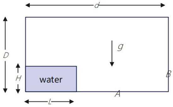
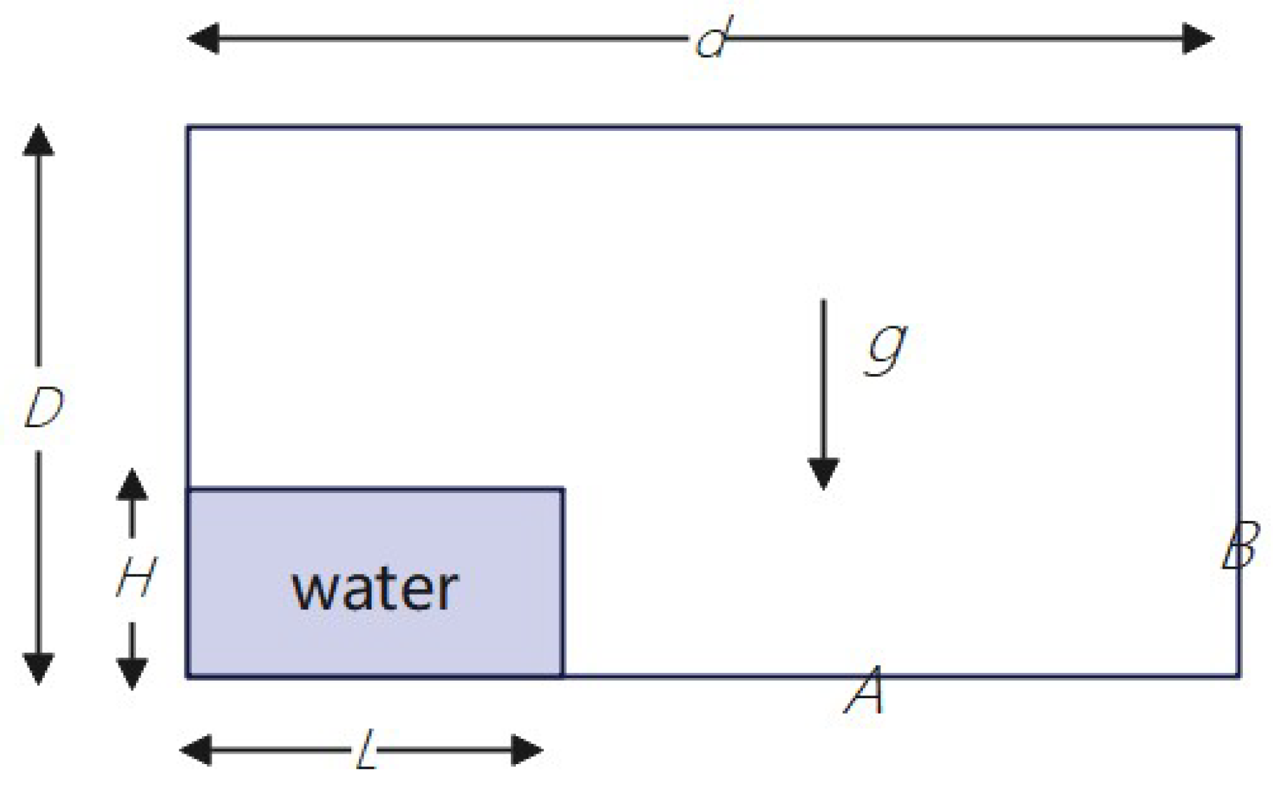
This dam break experiment is based on the theoretical framework proposed by Colagrossi et al., employing a two-dimensional numerical modeling approach that has become a widely adopted standard benchmark case in the field of dam break flow simulation. In computational fluid dynamics, simulation results can often be refined, for instance, by introducing artificial viscosity [29] or normalized density [30]. The initial state and computational model of the two-dimensional dam break are illustrated in Figure 1. Dimensionless time T is used to describe the fluid dynamics process. This study focused on analyzing water level variations at point A (3.721H, 0) and pressure fluctuations at point B (5.366H, 0.192H), comparing them with the numerical simulation results from DualSPHysics, JOSEPHINE [31], and Colagrossi [32], as well as experimental data from Zhou [33]. Key parameter settings included gravitational acceleration g of 9.81 m/s² and a water density of 1000 kg/m³.

Figure 1. Dam break experiment model diagram.

Figure 1 illustrates the initial configuration, with dam height of H and length L = 2H. The rectangular container has dimensions of length d = 5.366H and height D = 3H. This study examined the water level variation at point A and pressure fluctuations at point B.

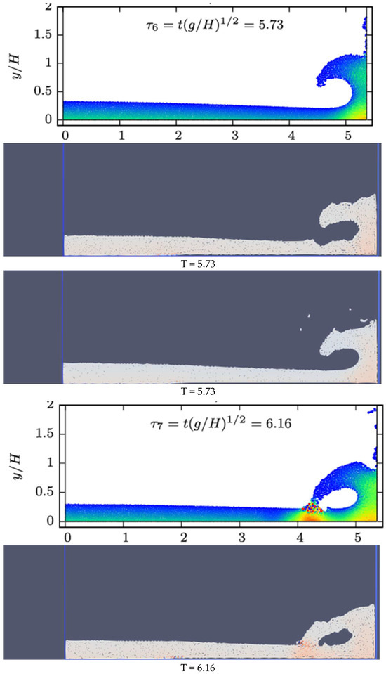
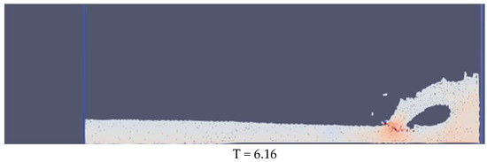
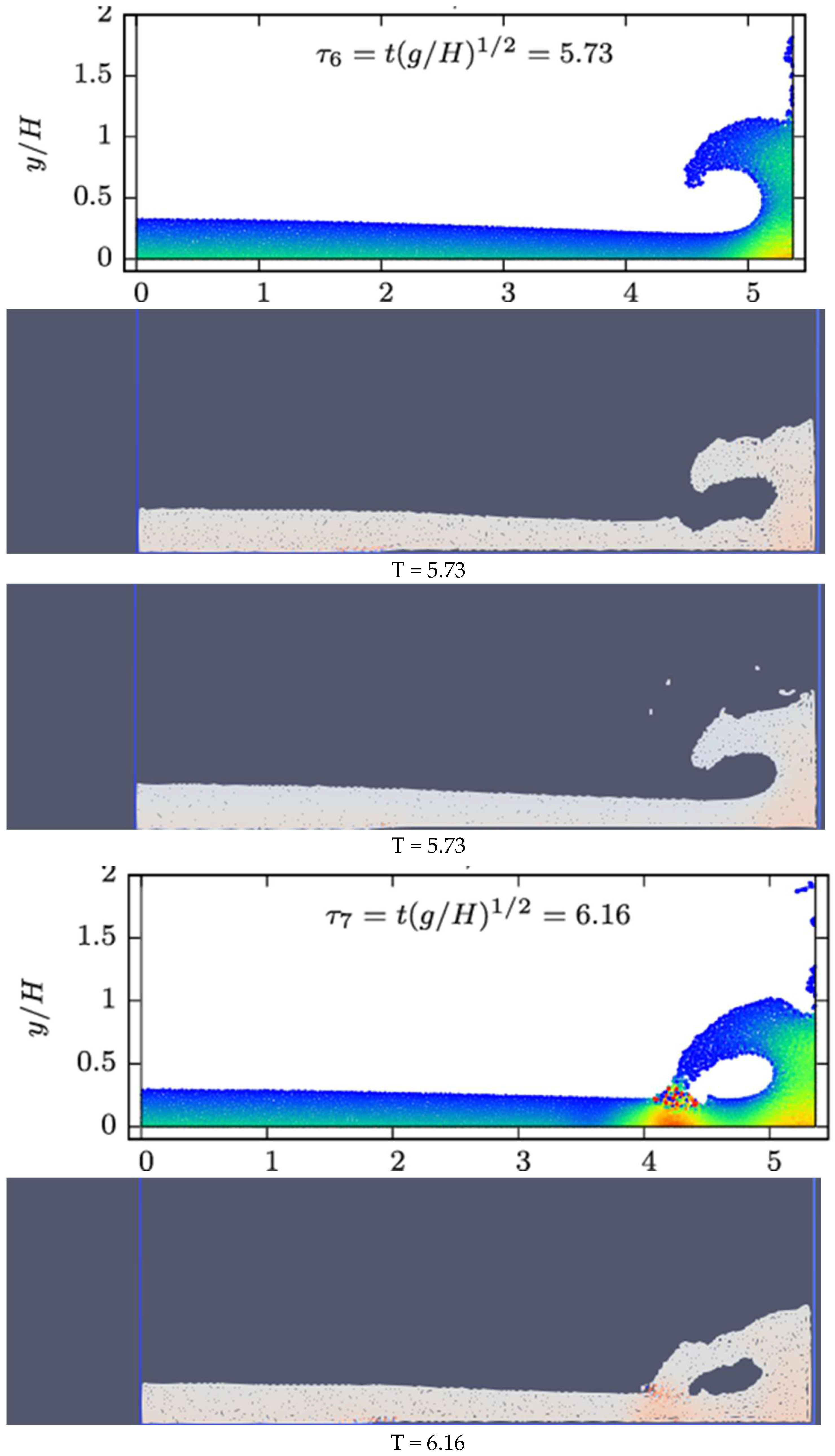
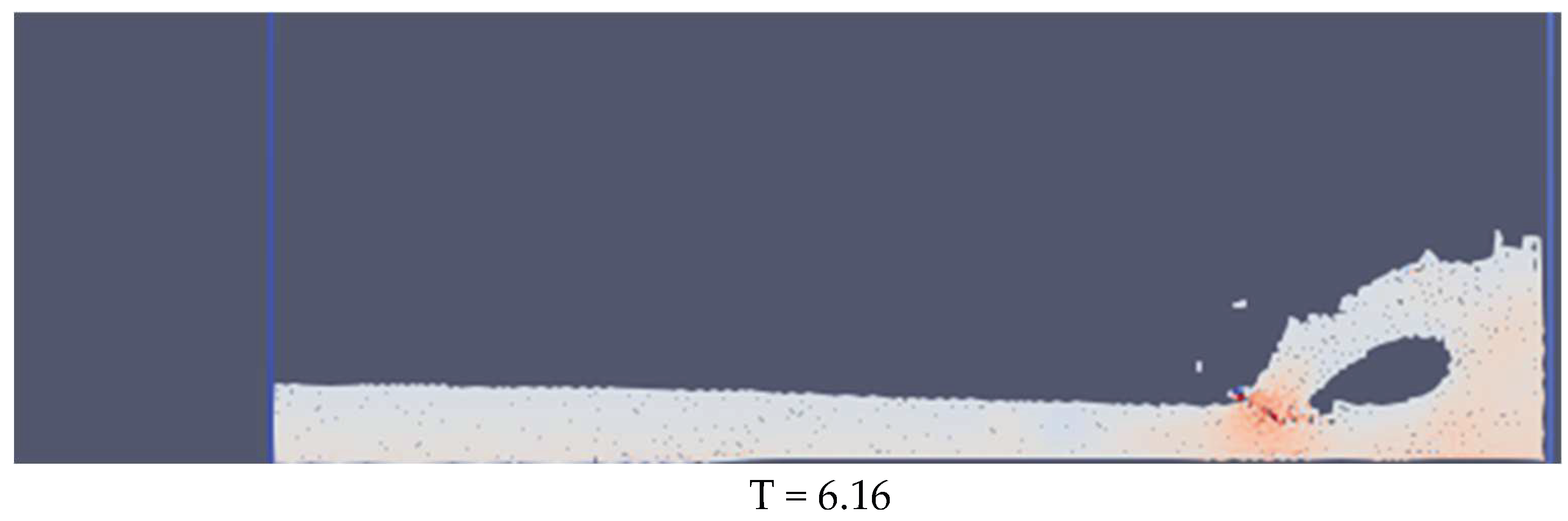
Figure 2 illustrates the state of the fluid at dimensionless time parameters of 5.73 and 6.16. From top to bottom, the results correspond to simulations from JOSEPHINE, DualSPHysics, and MSPH-DEM. It can be observed that the MSPH-DEM simulation results exhibit a closer alignment with experimental data in terms of cavity surface characteristics.

Figure 2. Comparison of dam break experiment results.

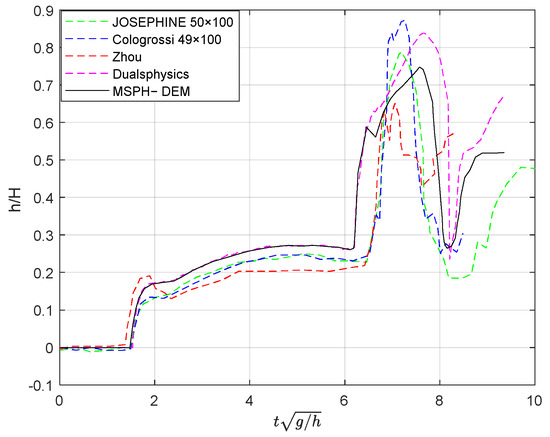
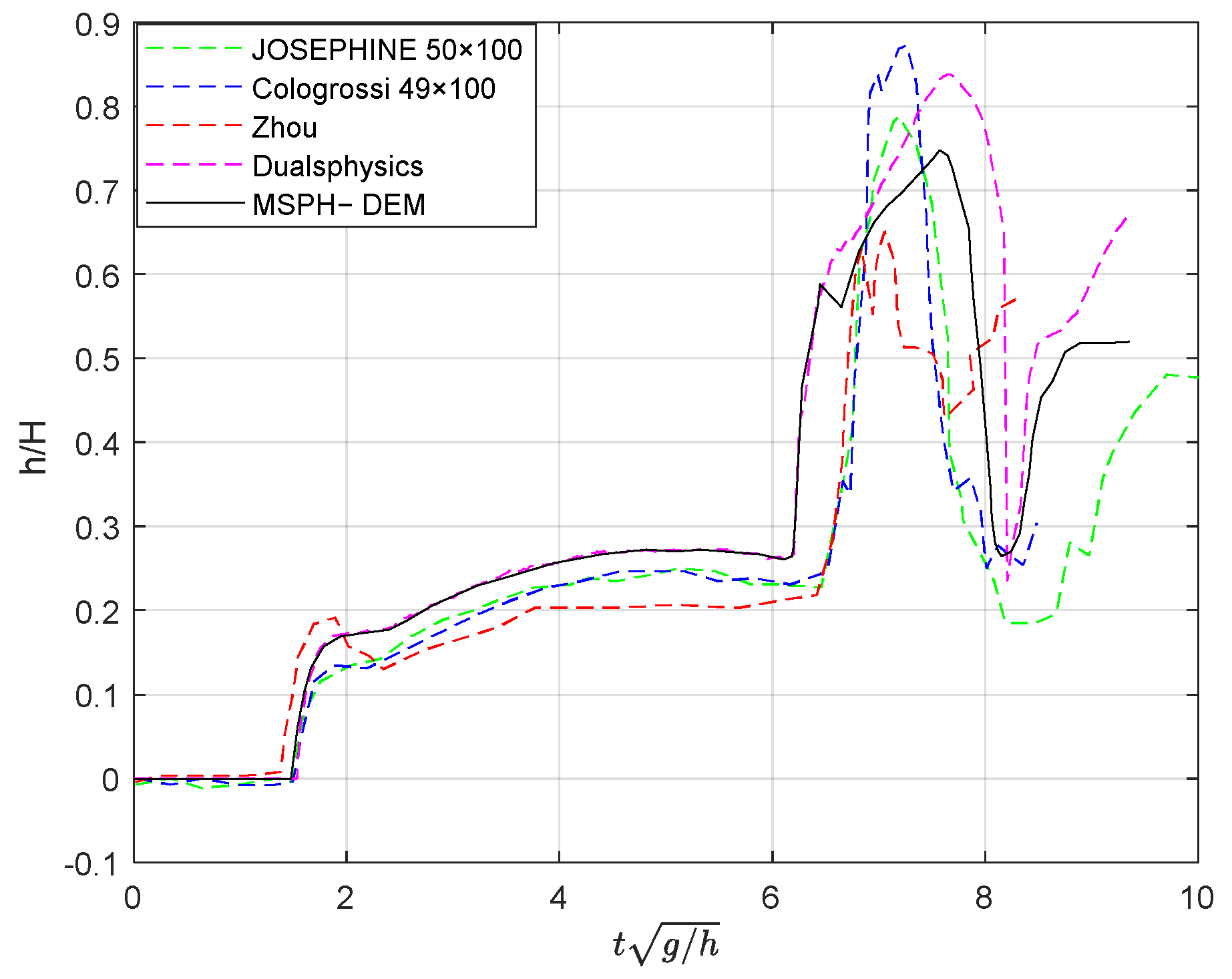
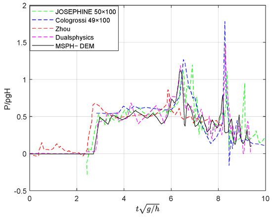
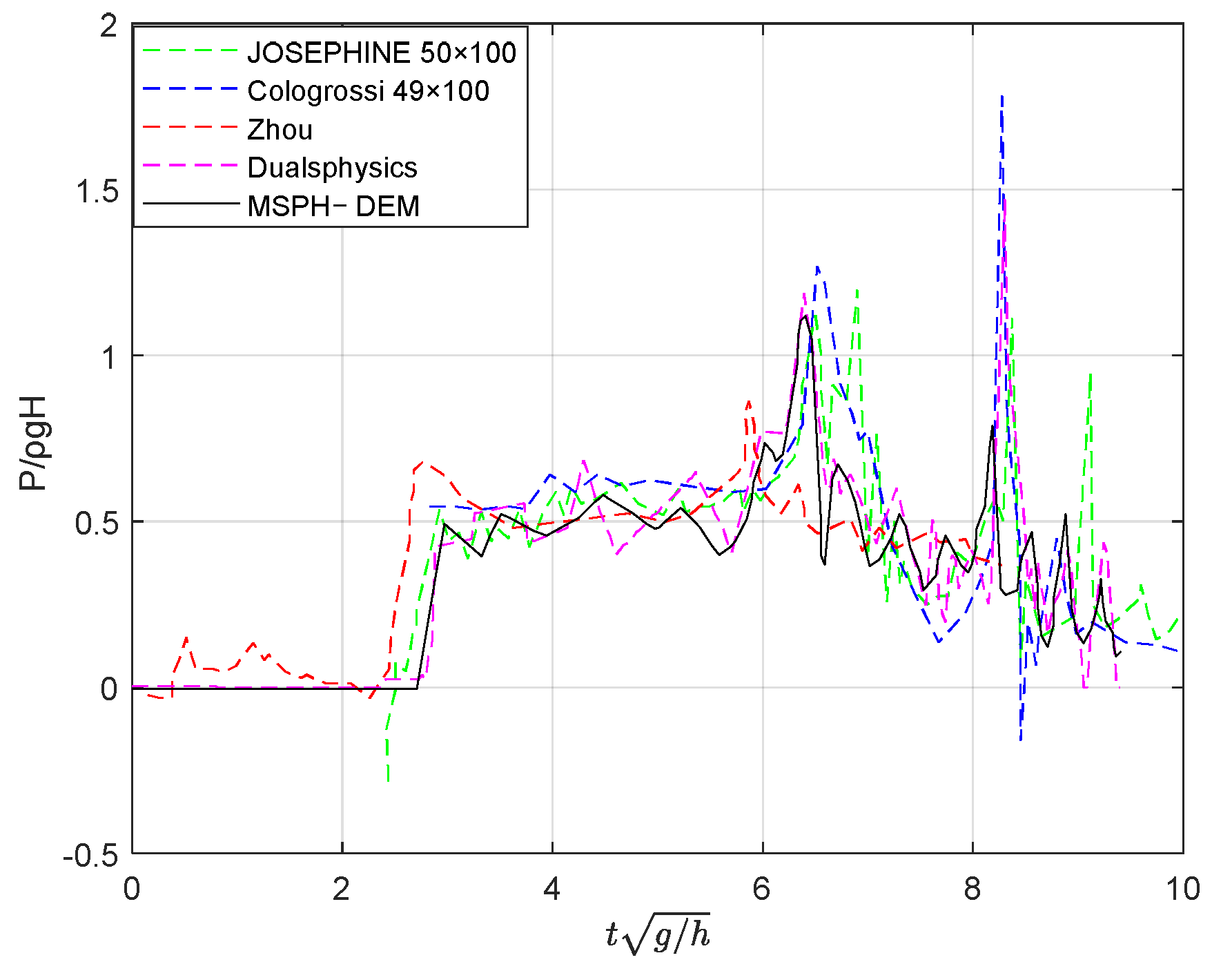
Figure 3 presents the numerical simulation results of the water level at point A, and Figure 4 shows the comparison of pressure data at point B, where the black solid line denotes the MSPH-DEM numerical simulation. The numerical simulation results indicate that MSPH-DEM exhibits excellent computational performance in the simulation of hydraulic characteristics. As reflected by the water level data comparison, the simulated values agree well with the experimental data. In terms of pressure characteristic simulation, MSPH-DEM successfully reproduces the transient conversion process from fluid kinetic energy to pressure energy, and the predicted pressure peak values are in good agreement with the experimental data.

Figure 3. Water level data comparison.

Figure 4. Pressure data comparison.

Specifically, taking the Cologrossi 49 × 100 case as the benchmark, in the prediction of the peak water level value, the peak prediction of the benchmark model is 0.87, that of the JOSEPHINE method is 0.78, while the proposed method improves it to 0.84. Compared with the JOSEPHINE method, the average relative error of the water level prediction is lower by 24.95%. For pressure prediction, the peak value predicted by the benchmark model is 1.78. In view of the deficiency of the JOSEPHINE method in predicting the second pressure peak (with a predicted value of 1.12), the proposed method optimizes it to 1.47, with the average relative error of pressure prediction reduced by 15.98%. This verifies its effect on improving computational accuracy. Such improvements are mainly attributed to the method optimizing numerical stability and computational precision.

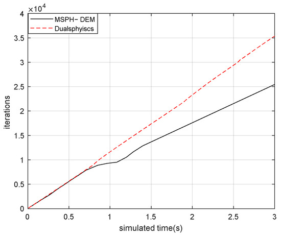
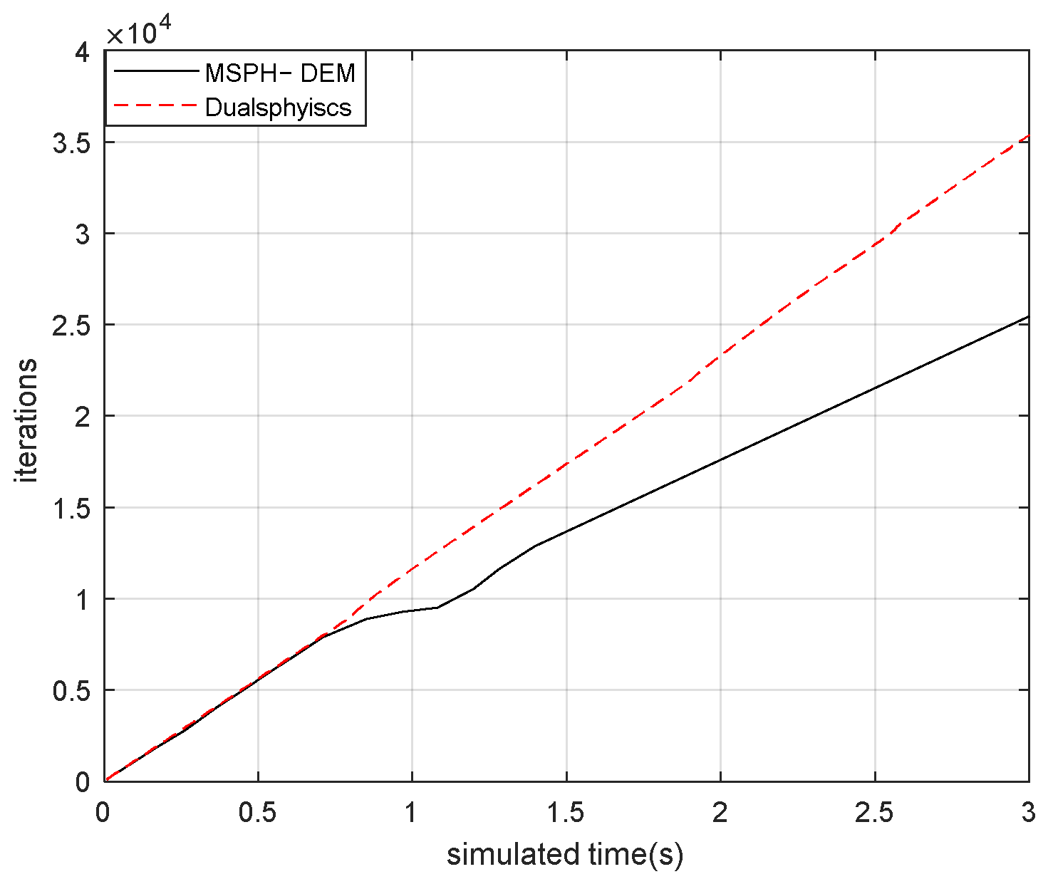
Figure 5 compares the curves of iteration number versus simulation time for two methods in dam break numerical simulation. The red dashed line represents the DualSPHysics method, and the black solid line denotes MSPH-DEM. The iteration number of MSPH-DEM is remarkably lower than that of the DualSPHysics method, and the gap between the two methods continues to widen as the simulation time increases. When the simulation time reaches 3 s, the total iteration number of the DualSPHysics method is approximately 35,388, while that of MSPH-DEM is only 25,497, achieving a reduction of 28.6%.

Figure 5. Comparison of dam break iteration number and simulation time.

5.2. Experimental Dam Impacting Cubic Structure

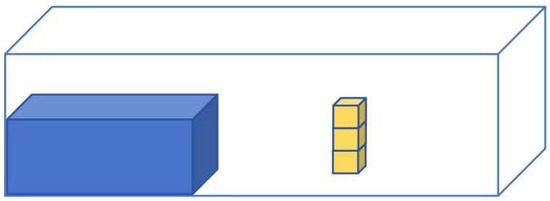
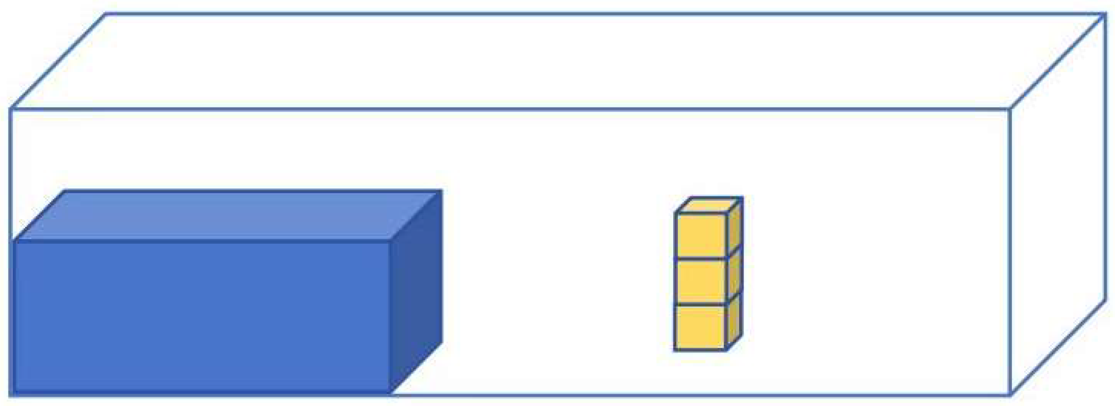
This experiment focused on the impact of a dam break on a cubic structure. To validate the coupled MSPH-DEM, the fluid–structure interaction process of the dam impacting the cube was simulated. Based on the studies by Shunying Ji (2019) [34] and Canelas et al. (2016) [10], the cube was positioned 1.7 m away from the initial water body, as illustrated in Figure 6. The simulation parameters are summarized in Table 1.

Figure 6. Dam break impacting block experiment. Blue represents water, and yellow represents the building block.

Table 1. Simulation parameters of dam impacting blocks.

Parameter	Value
Water tank: length × height × width	8 m × 0.7 m × 1 m
Cube size	0.15 m × 0.15 m ×0.15 m
Dilated radius of cube	0.01 m
Density of cube	800 kg/m3
Distance between cubes to water	1.7 m
Friction coefficient of water tank	0.35
Friction coefficient of cube	0.45
Poisson’s ratio of cube	0.3
Water size	3.5 m × 0.7 m × 0.4 m

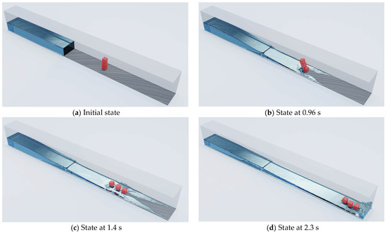
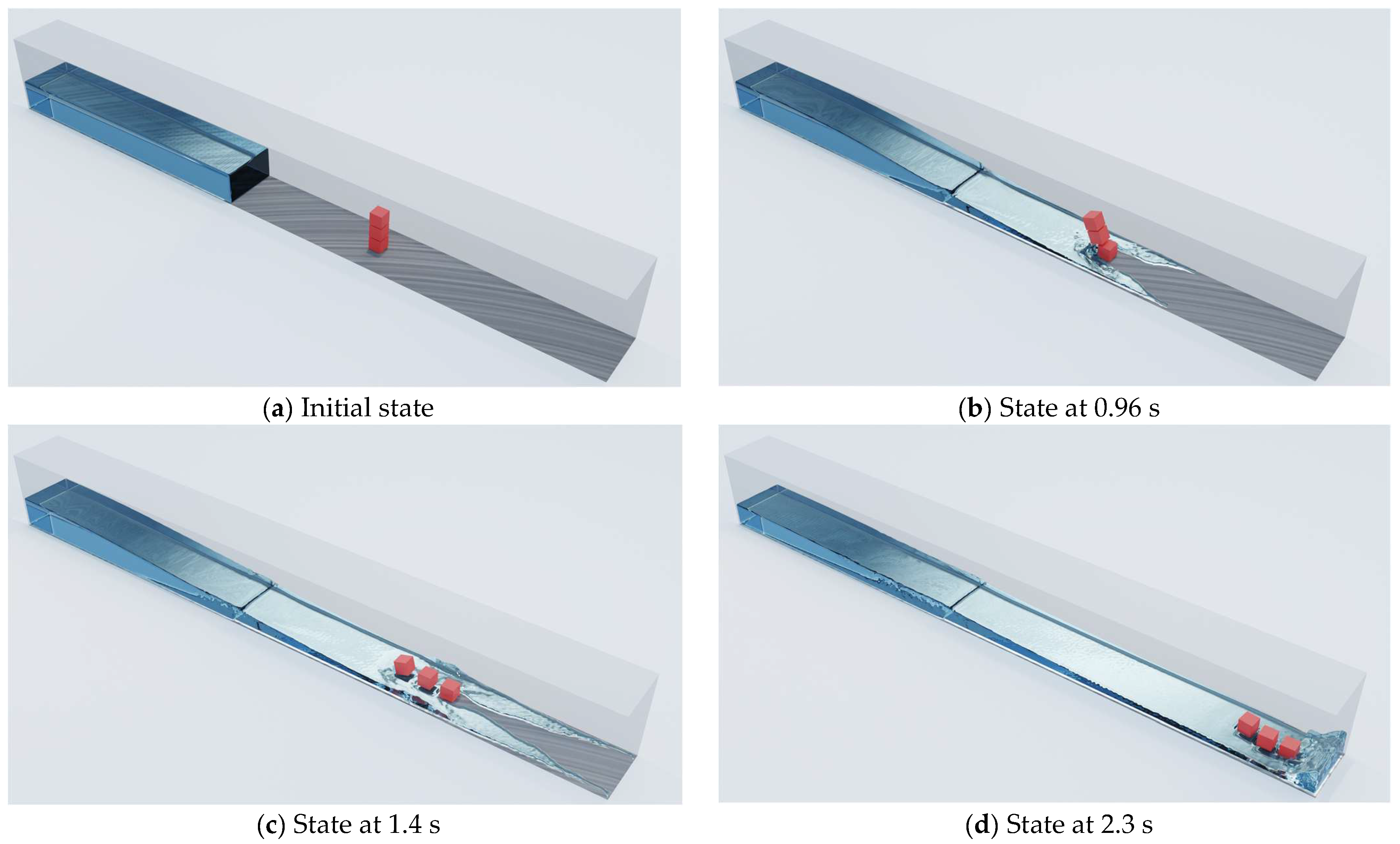
Figure 7 shows the process of a dam break flow impacting three cubic structures, simulated using MSPH-DEM. In the figure, Figure 7a–d correspond to the simulated states at four time instants: 0 s, 0.96 s, 1.4 s, and 2.3 s, respectively. Under the impact of the fluid, the cubic structures collapse and subsequently undergo gradual sliding displacement due to the sustained flow action.

Figure 7. Simulation results of dam break with three cubes.

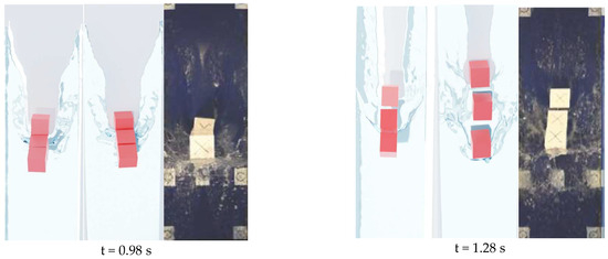
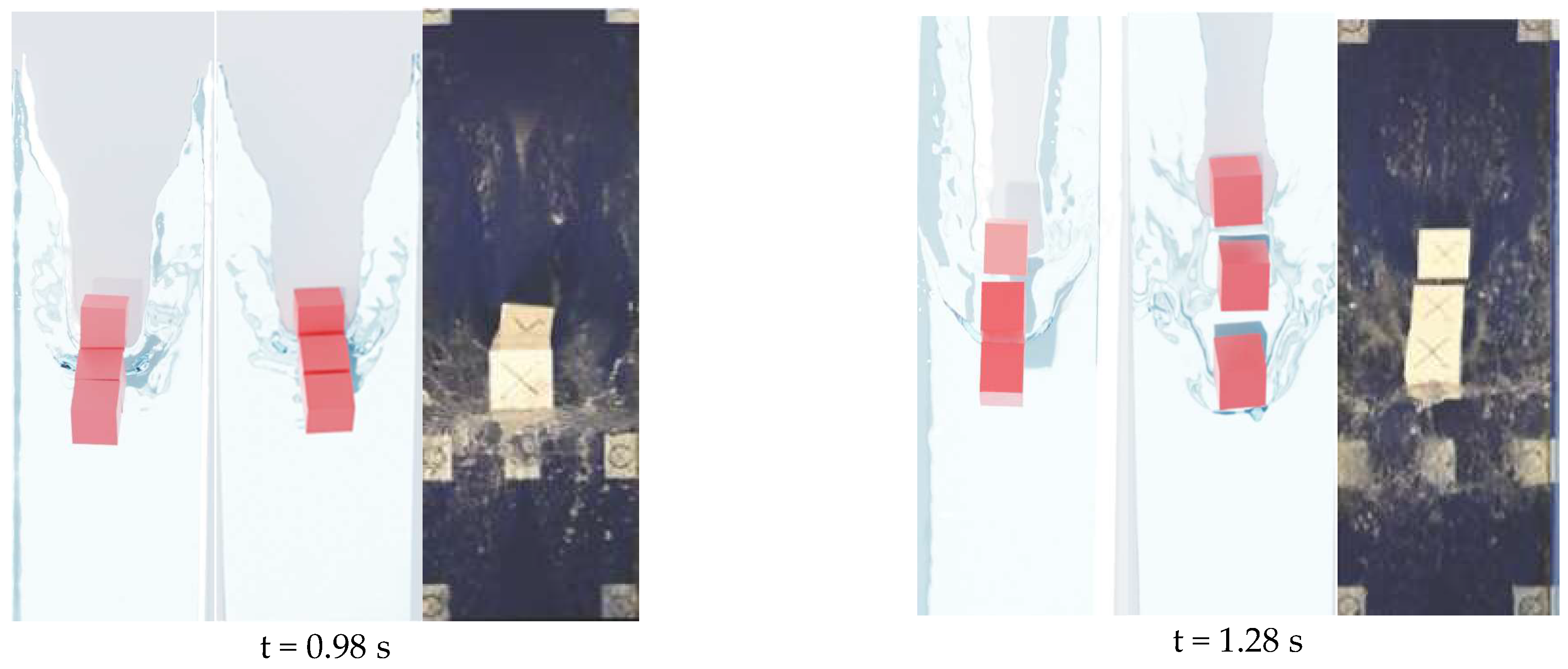
Figure 8 displays a comparison between MSPH-DEM and DualSPHysics simulation results alongside the experimental data from Canelas et al. (2016) [10] at two different time points, arranged from left to right. It can be observed that the fluid–structure interaction phenomena simulated by MSPH-DEM align more closely with the experimental results of Canelas.

Figure 8. Top view of dam break impact on blocks.

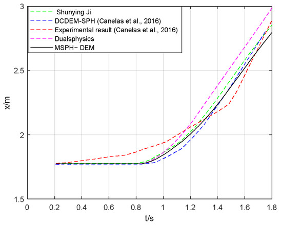
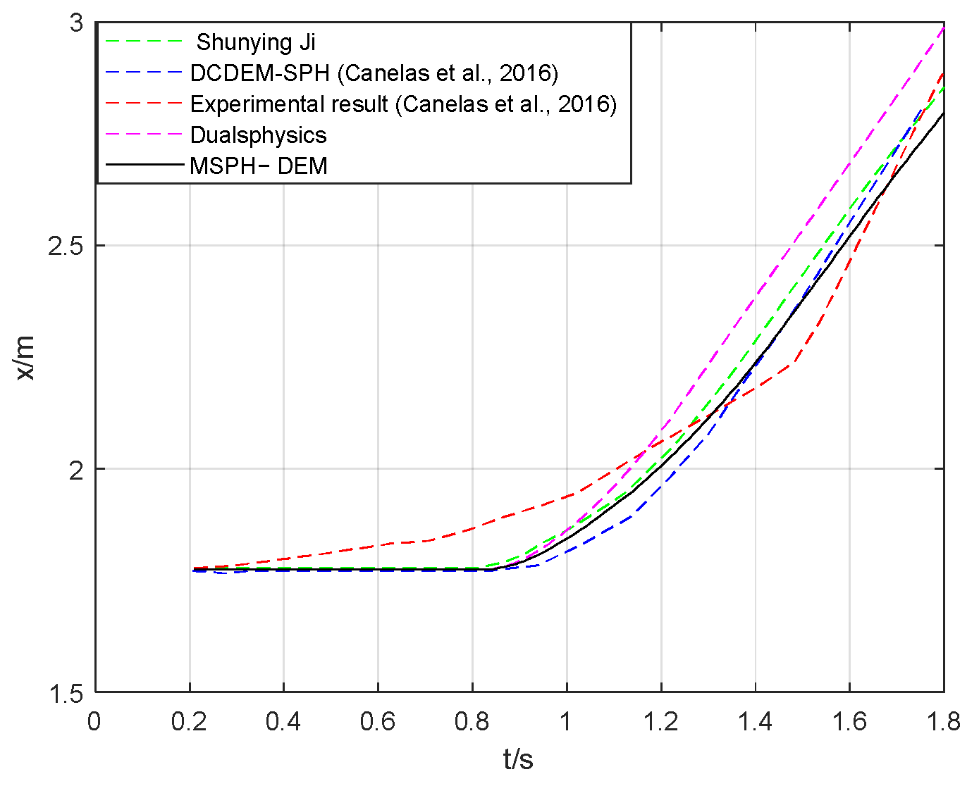
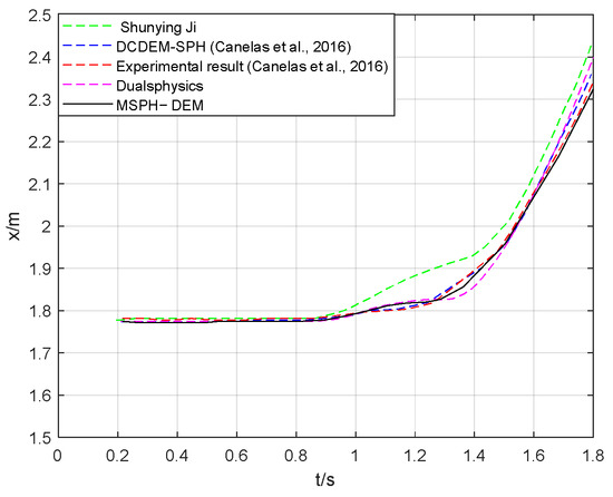
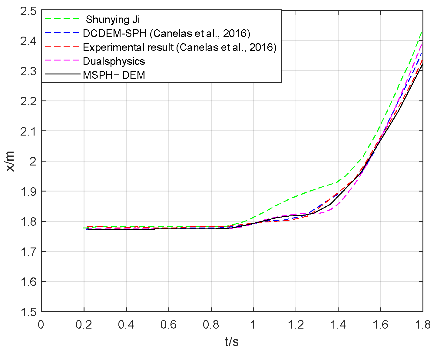
Figure 9 and Figure 10 present comparisons between the simulation results and experimental data for the displacement in the x-direction of the bottom and top cubes, respectively. In the figures, the black solid line represents the simulation results from MSPH-DEM, while the red dashed line corresponds to the experimental results from Canelas. The results indicate that after approximately 0.8 s, when the fluid impacts the cubes, the cubes move with a constant acceleration under the force of the water flow. While some discrepancies exist in the displacement of the bottom cube due to the combined effects of the interactions between the cubes and the tank, the MSPH-DEM results generally align more closely with Canelas’ experimental data than the simulation results from DualSPHysics.

Figure 9. Bottom block value.

Figure 10. Top block value.

5.3. Dam Break Impact on a Baffle Experiment

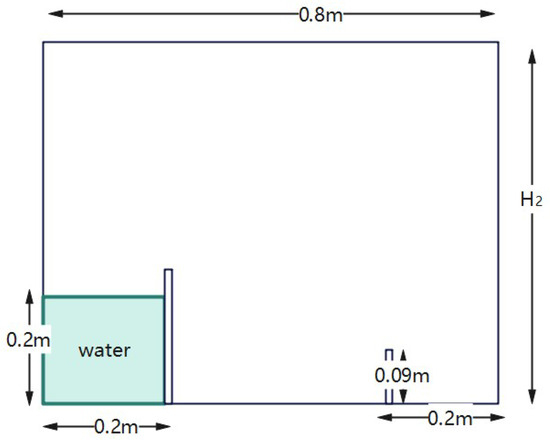
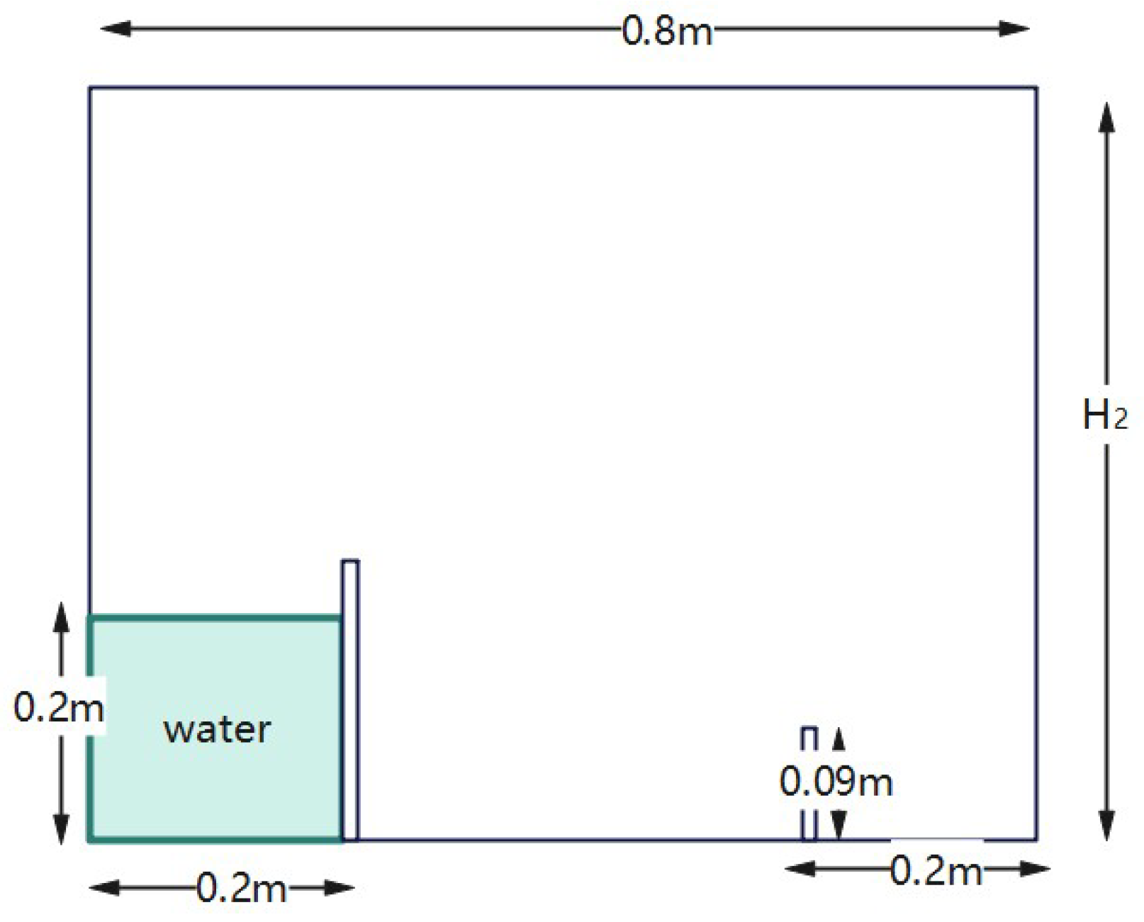
This experiment focused on the multiphase fluid–structure interaction phenomenon of dam break flow impacting an elastic baffle with an initial water depth of H = 0.2 m. The experimental setup is based on the design by Liao et al. [35]. The total length of the flume was 0.8 m, and the elastic baffle was fixed on the right side of the flume, 0.2 m away from the vertical wall. H2 was greater than the water depth. The baffle was made of rubber with a density of 1161.54 kg/m³, a Young’s modulus of 3.50 MPa, and a Poisson’s ratio of 0.45, as shown in Figure 11.

Figure 11. Model diagram of dam break impacting plate.

During the initial stage of the experiment, the water in the left section of the flume was blocked by a gate, which was gradually lifted following a specific motion pattern to trigger the dam-break flow. After forming a water tongue, the flow moved toward the right-side elastic baffle and impacted it. Subsequently, the flow overtopped the baffle and struck the right wall of the flume, forming trapped bubbles between the baffle, the right wall, and the flow. During the experiment, by recording the horizontal displacements of two markers at different heights (Marker 1 at 0.0875 m and Marker 2 at 0.065 m from the flume bottom) along the centerline of the baffle, combined with the observation of the flow morphology, the characteristics of the flow during the initial impact stage, the process of bubble entrapment and collapse, and the elastic response of the baffle were analyzed.

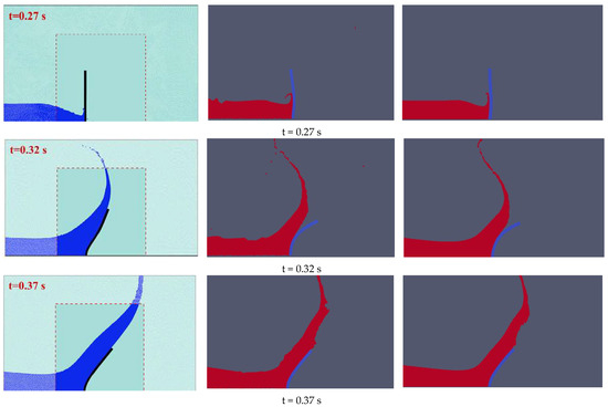
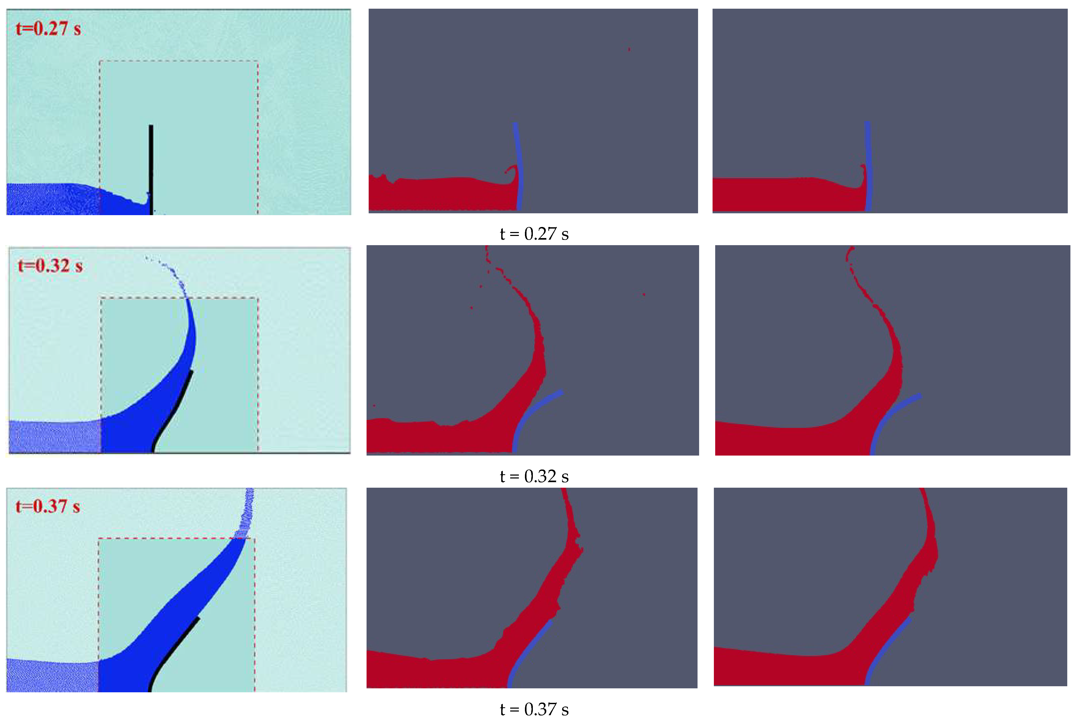
Figure 12 shows the simulated states at 0.27 s, 0.32 s, and 0.37 s. From top to bottom, the images represent the simulation diagrams produced with Sun, DualSPHysics, and MSPH-DEM. It can be observed from the figure that the surface of the MSPH-DEM simulation diagram is smoother than that of DualSPHysics and closer to the simulation result of Sun.

Figure 12. Comparison of simulation results for dam break impacting plate model.

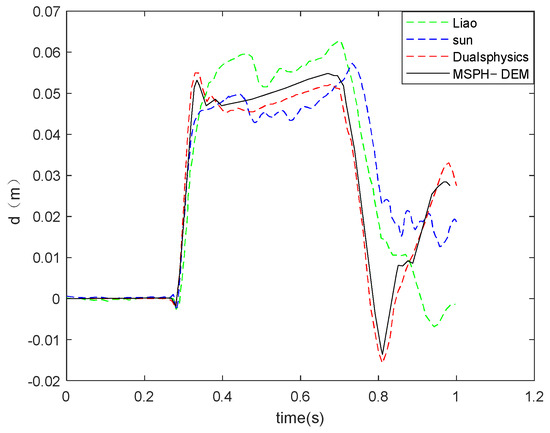
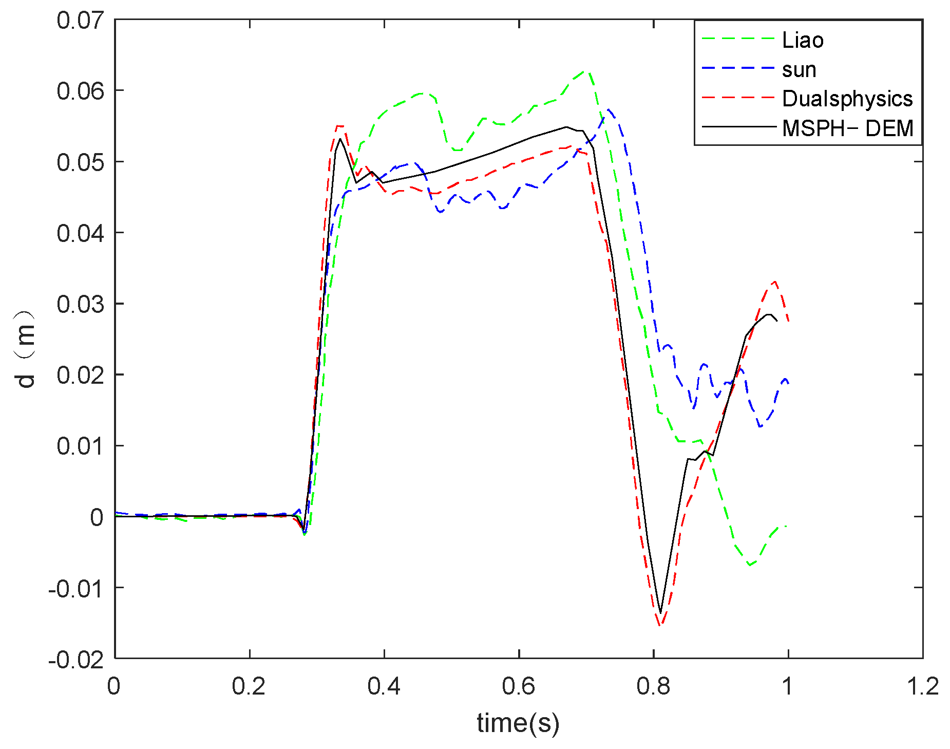
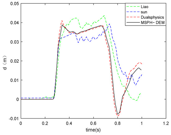
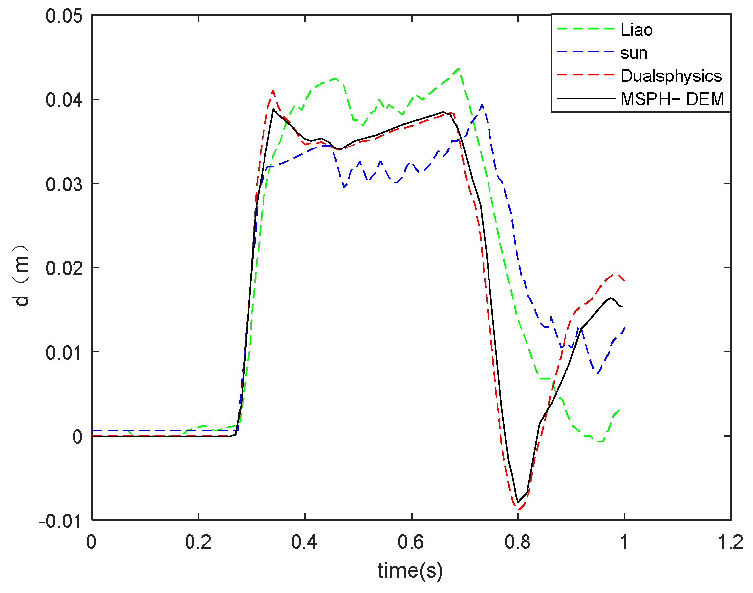
The analysis of numerical simulation results indicates that MSPH-DEM can effectively simulate the dam break impacting a baffle experiment. As shown in Figure 13 and Figure 14, the MSPH-DEM simulation results, represented by the black solid line, are compared with the experimental results of Liao et al. [35], the simulation results of Sun et al. [36], and the DualSPHysics simulation results. The MSPH-DEM simulation accurately reproduces the temporal evolution of the horizontal displacements at Marker 1 and Marker 2. Although slight deviations exist between the simulation and experimental data, the overall dynamic response trend is consistent with the experimental observations. In Figure 13, taking the SUN experimental data as the reference true value, the calculated average relative error of the DualSPHysics simulation results is 18.72%, while that of the MSPH-DEM simulation results is only 6.35%. MSPH-DEM exhibits a much lower average relative error than the DualSPHysics method and achieves a higher overall agreement with the experimental data. Moreover, it shows better consistency in numerical trends as well as key peak and valley values. With significantly improved simulation accuracy, MSPH-DEM can better reproduce the real physical process.

Figure 13. Horizontal displacement variation for Marker 1.

Figure 14. Horizontal displacement variation for Marker 2.

It is worth noting that the simulation successfully captures the variations in the horizontal displacement of the elastic baffle. This result demonstrates that, compared to DualSPHysics, MSPH-DEM exhibits higher agreement in simulating fluid–structure interaction problems and can accurately reflect the dynamic response behavior of elastic structures under fluid action.

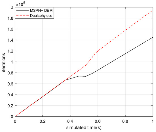
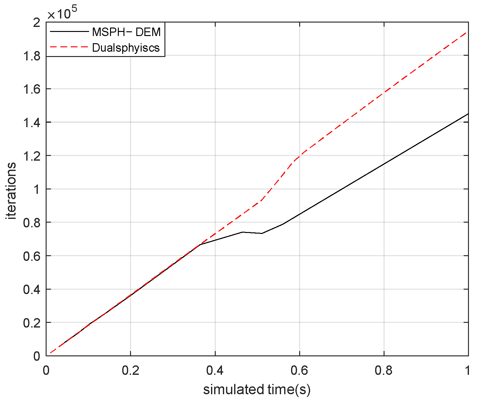
From Figure 15, MSPH-DEM significantly outperforms the DualSPHysics method in terms of computational efficiency in dam break numerical simulations. Although the number of iterations for both methods increases with simulation time, the growth rate of iterations for MSPH-DEM is markedly slower, and the gap between the two methods continues to widen as the simulation progresses. At a simulation time of 1 s, the number of iterations for the DualSPHysics method is 2 × 10⁵, while that of MSPH-DEM is 1.45 × 10⁵. This demonstrates that MSPH-DEM can substantially reduce computational iteration costs while advancing the simulation process, effectively improving the overall efficiency of numerical simulations. It exhibits a clear efficiency advantage when dealing with long-duration fluid or fluid–structure interaction problems, making it more suitable for large-scale and long-term engineering numerical simulation scenarios.

Figure 15. Comparison diagram of time and iteration number for dam-break impact on single plate.

5.4. Visual Effects of 3D Fluid–Structure Interaction

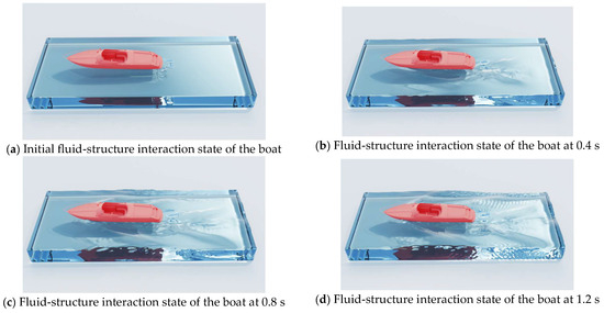
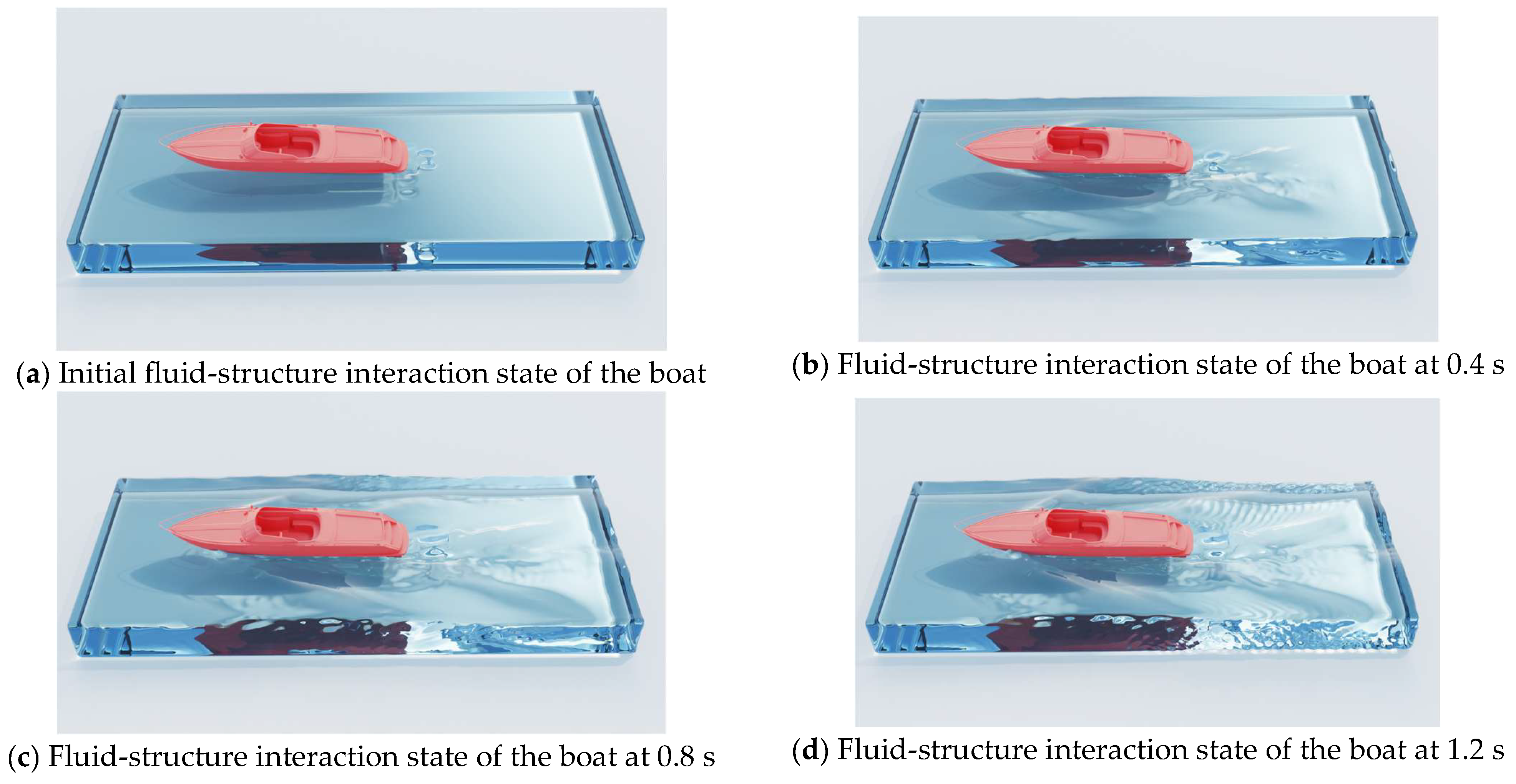
An analysis of the graphical results demonstrates the capability of MSPH-DEM in simulating three-dimensional fluid–structure interaction problems. In Figure 16, Figure 16a–d represent the simulated states at time instants of 0 s, 0.4 s, 0.8 s, and 1.2 s, respectively. The method successfully reproduces the fluid–structure interaction process of ship motion under the influence of free inflow (1.5 m/s), clearly capturing wave generation at both the bow and stern as the vessel advances, and accurately reflects the impact of the fluid on the hull as well as its dynamic response.

Figure 16. Fluid–structure interaction between water flow and small boat.

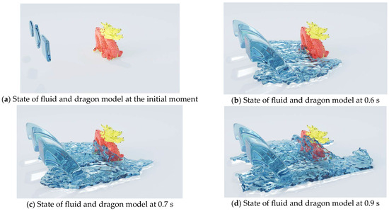
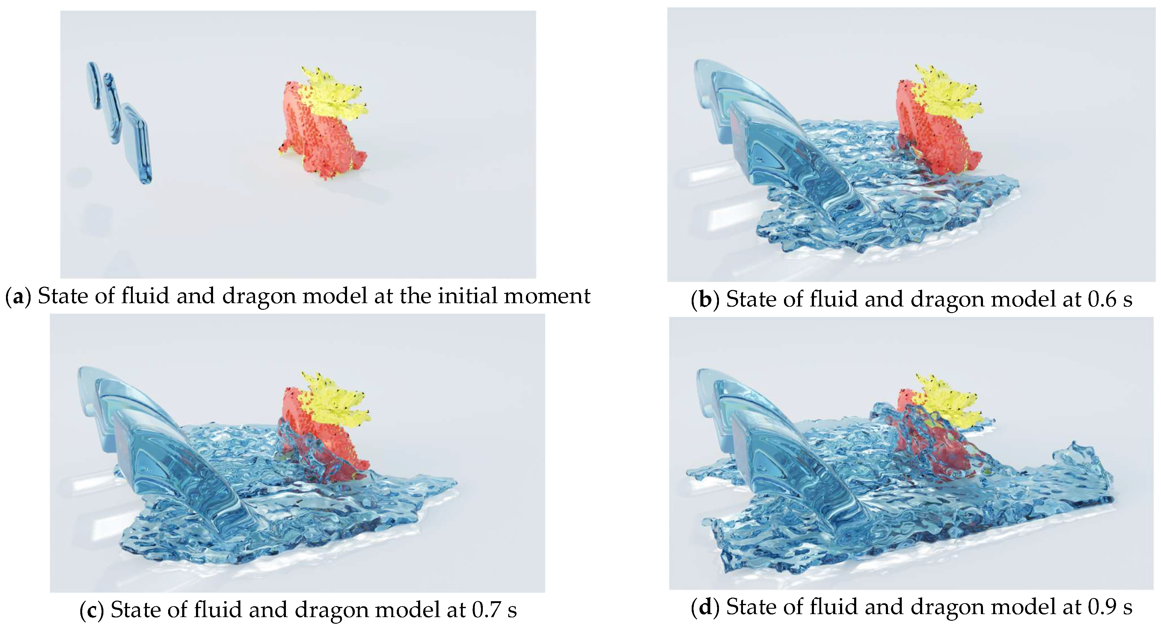
Figure 17 presents a fluid impact simulation of a dragon-shaped solid model using three different inlet configurations (square, diamond, and circular), aiming to investigate the dynamic response mechanisms of complex biological geometries under fluid–structure interaction. The dragon model features multiscale curvature and asymmetric geometric characteristics. By impacting the dragon-shaped model, the patterns of the fluid acting on the solid surface were analyzed, providing a theoretical basis for bionic design and fluid–structure interaction control. In Figure 17, Figure 17a–d correspond to the simulated states at four time instants: 0 s, 0.6 s, 0.7 s, and 0.9 s.

Figure 17. Fluid–structure interaction between water flow and dragon model.

6. Conclusions

MSPH-DEM, proposed in this study, effectively mitigates issues such as pressure oscillations by integrating the moving least squares (MLS) method within the DualSPHysics framework. While maintaining weakly compressible characteristics, the simulation results demonstrate closer agreement with experimental data. The numerical experiments indicate that (1) the stability of the pressure field is improved in dam break simulations; (2) the results of the dam break case show good agreement with the experimental data from Canelas et al.; and (3) the horizontal displacements of the two marker points in the dam break impacting a baffle experiment closely match the experimental results from Liao et al. Theoretically, this method can accurately correct the kernel function gradient and precisely solve the coupling phenomena in fluid–structure interaction. However, in practical applications, further optimization is still required due to influences such as boundary effects. The current method is applicable to engineering problems such as debris flows and particle screening, but, for complex scenarios involving ultrafine particles or high-speed flows, extended research incorporating turbulence models or non-Newtonian fluid constitutive equations is needed. However, the proposed MSPH-DEM still has some limitations. For complex 3D geometries with multi-curvature surfaces and non-spherical particles, the contact detection and coupling accuracy need to be further improved. In addition, the method is sensitive to parameters such as smoothing length and contact stiffness, which may affect the stability of pressure and displacement results. Future research will focus on improving 3D coupling for complex geometries and non-spherical DEM particles and conducting more experimental validation for engineering scenarios such as debris flows and landslide surges.

References

- Benz, W.; Hills, J. Three-dimensional hydro-dynamical simulations of colliding stars. III: Collisions and tidal captures of unequal-mass main-sequence stars. Astrophys. J. 1992, 389, 546–557. [Google Scholar] [CrossRef] [Scilit]
- Monaghan, J.J.; Gingold, R. Shock simulation by the particle method SPH. J. Comput. Phys. 1983, 52, 374–389. [Google Scholar] [CrossRef] [Scilit]
- Frederic, A.; James, C. Smoothed particle hydrodynamics calculations of stellar interactions. J. Comput. Appl. Math. 1999, 109, 213–230. [Google Scholar] [CrossRef] [Scilit]
- Lee, C.; Lee, H.; Ann, H.; Kwon, K.H. Smoothed particle hydrodynamic simulations of Galactic gaseous disk with bar: Distribution and kinematic structure of molecular clouds toward the Galactic center. Astrophys. J. 1999, 513, 242–251. [Google Scholar] [CrossRef] [Scilit]
- Becker, M.; Teschner, M. Weakly compressible SPH for free surface flows. In Proceedings of the Eurographics/ACM SIGGRAPH Symposium on Computer Animation, San Diego, CA, USA, 2–4 August 2007; pp. 209–217. [Google Scholar]
- Canelas, R.B.; Domínguez, J.M.; Crespo, A.J.C.; Gómez-Gesteira, M.; Ferreira, R.M.L. A Smooth Particle Hydrodynamics discretization for the modelling of free surface flows and rigid body dynamics. Int. J. Numer. Methods Fluids 2015, 78, 581–593. [Google Scholar] [CrossRef] [Scilit]
- Gingold, J.J.; Monaghan, J.J. Smoothed particle hydrodynamics: Theory and application to non-spherical stars. Mon. Not. R. Astron. Soc. 1977, 181, 375–389. [Google Scholar] [CrossRef] [Scilit]
- Lucy, L.B. A numerical approach to the testing of the fission hypothesis. Astron. J. 1977, 82, 1013–1024. [Google Scholar] [CrossRef] [Scilit]
- Govender, N.; Wilke, D.N.; Kok, S. Blaze-DEMGPU: Modular high performance DEM framework for the GPU architecture. SoftwareX 2016, 5, 62–66. [Google Scholar] [CrossRef] [Scilit]
- Canelas, R.B.; Crespo, A.J.C.; Domínguez, J.M.; Ferreira, R.M.L.; Gómez-Gesteira, M. SPH–DCDEM model for arbitrary geometries in free surface solid–fluid flows. Comput. Phys. Commun. 2016, 202, 131–140. [Google Scholar] [CrossRef] [Scilit]
- You, Y.; Ma, H.; Xu, L. Investigation of the vibration sorting of non-spherical particles based on DEM simulation. Powder Technol. 2018, 325, 316–332. [Google Scholar] [CrossRef] [Scilit]
- Bambauer, F.; Wirtz, S.; Scherer, V. Transient DEM-CFD simulation of solid and fluid flow in a three-dimensional blast furnace model. Powder Technol. 2018, 334, 53–64. [Google Scholar] [CrossRef] [Scilit]
- Shen, Z.; Wang, G.; Huang, D. A resolved CFD-DEM coupling model for modeling two-phase fluids interaction with irregularly shaped particles. J. Comput. Phys. 2022, 448, 110695. [Google Scholar]
- Ma, H.; Zhou, L.; Liu, Z. A review of recent development for the CFD-DEM investigations of non-spherical particles. Powder Technol. 2022, 412, 117972. [Google Scholar]
- Dhairya, R.V.; Cummins, S.J.; Rudman, M. Collisional SPH: A method to model frictional collisions with SPH. Appl. Math. Model. 2021, 94, 13–35. [Google Scholar] [CrossRef] [Scilit]
- Peng, C.; Zhan, L.; Wu, W. A fully resolved SPH-DEM method for heterogeneous suspensions with arbitrary particle shape. Powder Technol. 2021, 387, 509–526. [Google Scholar] [CrossRef] [Scilit]
- Zhang, J.; Wang, B. Numerical simulation and experimental study of fluid–structure interactions in elastic structures based on the SPH method. Ocean Eng. 2024, 301, 117523. [Google Scholar] [CrossRef] [Scilit]
- Islam, M.R.I. SPH-based framework for model-ling fluid–structure interaction problems with finite deformation and fracturing. Ocean Eng. 2024, 294, 116722. [Google Scholar] [CrossRef] [Scilit]
- Zhi-Bin, W.; Rong, C.; Hong, W. An overview of smoothed particle hydrodynamics for simulating multiphase flow. Appl. Math. Model. 2016, 40, 9625–9655. [Google Scholar] [CrossRef] [Scilit]
- Zheng, B.X.; Chen, Z. A multiphase smoothed particle hydro dynamics model with lower numerical diffusion. J. Comput. Phys. 2019, 382, 177–201. [Google Scholar] [CrossRef] [Scilit]
- Fernández-Gutiérrez, D.; Zohdi, T.I. Delta Voronoi smoothed particle hydrodynamics, δ-VSPH. J. Comput. Phys. 2020, 401, 109000. [Google Scholar] [CrossRef] [Scilit]
- Chen, C.; Zhang, A.-M. SPH simulations of water entry problems using an improved boundary treatment. Ocean Eng. 2021, 238, 109679. [Google Scholar] [CrossRef] [Scilit]
- Gao, T.; Qiu, H. A block-based adaptive particle refinement SPH method for fluid–structure interaction problems. Comput. Methods Appl. Mech. Eng. 2022, 399, 115356. [Google Scholar] [CrossRef] [Scilit]
- Khayyer, A.; Shimizu, Y. A 3D SPH-based entirely Lagrangian meshfree hydroelastic FSI solver for anisotropic composite structures. Appl. Math. Model. 2022, 112, 560–613. [Google Scholar] [CrossRef] [Scilit]
- Zou, L.; Sun, J.Z.; Sun, Z. Study of two free-falling spheres interaction by coupled SPH–DEM method. Eur. J. Mech. B/Fluids 2022, 92, 49–64. [Google Scholar] [CrossRef] [Scilit]
- Monaghan, J.J. Smoothed particle hydrodynamics. Annu. Rev. Astron. Astrophys. 1992, 30, 543–574. [Google Scholar] [CrossRef]
- Monaghan, J.J.; Kos, A. Solitary waves on a Cretan beach. J. Waterw. Port. Coast. Ocean Eng. 1999, 125, 145–154. [Google Scholar] [CrossRef] [Scilit]
- Cummins, S.J.; Cleary, P.W. Using distributed contacts in DEM. Appl. Math. Model. 2011, 35, 1904–1914. [Google Scholar] [CrossRef] [Scilit]
- Colagrossi, A.; Landini, M. Numerical simulation of interfacial flows by smoothed particle hydrodynamics. J. Comput. Phys. 2003, 191, 448–475. [Google Scholar] [CrossRef] [Scilit]
- Bonet, J.; Lok, T.-S.L. Variational and momentum preservation aspects of smooth particle hydrodynamic formulations. Comput. Methods Appl. Mech. Eng. 1999, 180, 97–115. [Google Scholar] [CrossRef] [Scilit]
- Cherfils, J.M.; Pinon, G.; Rivoalen, E. JOSEPHINE: A parallel SPH code for free-surface flows. Comput. Phys. Commun. 2012, 183, 1468–1480. [Google Scholar] [CrossRef] [Scilit]
- Molteni, D.; Colagrossi, A. A simple procedure to improve the pressure evaluation in hydrodynamic context using the SPH. Comput. Phys. Commun. 2009, 180, 861–872. [Google Scholar] [CrossRef] [Scilit]
- Zhou, Z.Q.; De Kat, J.O.; Buchner, B. A nonlinear 3-d approach to simulate green water dynamics on deck. In Proceedings of the 7th International Conference on Numerical Ship Hydrodynamics, Nantes, France, 19–22 July 1999. [Google Scholar]
- Ji, S.; Chen, X.; Liu, L. Coupled DEM-SPH Method for Interaction between Dilated Polyhedral Particles and Fluid. Math. Probl. Eng. 2019, 2019, 4987801. [Google Scholar] [CrossRef] [Scilit]
- Liao, K.; Hu, C.; Sueyoshi, M. Free surface flow impacting on an elastic structure: Experiment versus numerical simulation. Appl. Ocean Res. 2015, 50, 192–208. [Google Scholar] [CrossRef] [Scilit]
- Sun, P.N.; Le, T.D.; Zhang, A.-M. Study of a complex fluid-structure dam-breaking benchmark problem using a multiphase SPH method with APR. Eng. Anal. Bound. Elem. 2019, 104, 240–258. [Google Scholar] [CrossRef] [Scilit]
Disclaimer/Publisher’s Note: The statements, opinions and data contained in all publications are solely those of the individual author(s) and contributor(s) and not of MDPI and/or the editor(s). MDPI and/or the editor(s) disclaim responsibility for any injury to people or property resulting from any ideas, methods, instructions or products referred to in the content. |
© 2026 by the authors. Licensee MDPI, Basel, Switzerland. This article is an open access article distributed under the terms and conditions of the Creative Commons Attribution (CC BY) license.