A Novel Lithology Recognition Framework Based on Auxiliary Classification-Guided Denoising Diffusion and Multi-Scale Deep Learning

Abstract

Lithology identification is a key task in petroleum geological exploration and development, essential for evaluating sweet spots and characterizing reservoirs. A significant challenge in lithology identification is the insufficient accuracy of traditional machine learning methods due to the uneven distribution of geological data categories. To address this, we propose a novel lithology identification framework combining a denoising diffusion model with auxiliary classification, a neural network with channel attention mechanisms, and a bidirectional Gated Recurrent Unit (GRU). The proposed framework first employs the Auxiliary Classification Denoising Diffusion Probabilistic Model (A-CDPM) to generate high-quality well log data, effectively balancing the data classes. Secondly, it utilizes a multi-scale convolutional model with channel attention mechanisms and a Bidirectional GRU classification model, which automatically adjusts feature weights and effectively integrates information from different well log data. Experimental results demonstrate that our method significantly improves lithology identification accuracy, achieving 86.66% on datasets from the Hugoton and Panoma fields in Kansas, USA. Compared to traditional methods, this framework substantially enhances recognition precision, providing a novel and effective solution for lithology identification in petroleum geological exploration.

1. Introduction

Lithology identification is a critical aspect of petroleum exploration and development, playing a vital role in sweet spot evaluation, reservoir characterization, reservoir interval division, and development planning [1,2,3,4]. In practical oil and gas exploration and development, lithology identification is challenged by strong formation heterogeneity, complex depositional structures, overlapping well-log responses, limited core availability, insufficient lithology labels, and uneven lithological distributions [5,6]. Reliable lithology labels are usually obtained from core observations, laboratory analysis, mud logging interpretation, or expert geological interpretation, which are costly, time-consuming, and difficult to obtain continuously along the whole well interval [7,8,9]. As a result, available labeled samples are often limited, and minority lithologies may be seriously underrepresented in the training dataset. In many reservoirs, these minority lithologies may occur only in thin interbeds or transitional zones, but they can still strongly influence reservoir connectivity, fluid migration, and reservoir quality [10]. Therefore, inaccurate identification of these lithologies may lead to biased reservoir characterization and unreliable sweet spot evaluation [11]. These practical challenges highlight the need for robust lithology identification methods capable of handling heterogeneous, label-limited, and imbalanced well-log data. Accordingly, improving lithology identification under complex and imbalanced well-log conditions is not merely a classification problem, but is directly related to the reliability of reservoir characterization, sweet spot prediction, and subsequent development decision-making.

Traditional lithology identification primarily relies on core analysis and well-log cross-plot analysis [12,13]. Core analysis involves geological experts examining core or lithology samples under a microscope and conducting physicochemical experiments to determine lithology [14]. While this method provides accurate information, it is costly and time-consuming. The well-log cross-plot analysis infers lithology by analyzing the relationships among multiple well-log curves. However, its accuracy is often limited by overlapping logging responses and formation heterogeneity, particularly in complex formations, where the errors in the intersection diagrams are significant, leading to lower classification accuracy [15,16].

In recent years, machine learning methods, especially deep learning techniques, have attracted increasing attention for data-driven lithology identification because they can automatically extract lithology-related features from large-scale well-log data and reduce reliance on manual interpretation [17]. Techniques such as Support Vector Machines (SVM) [18], decision trees, and random forests have shown promising results in some lithology classification tasks [19]. However, traditional machine learning models and methods are constrained by data quality, with model predictions tending to be biased toward the majority class and failing to capture the minority classes comprehensively. To address this issue, researchers have proposed various approaches, such as oversampling, undersampling, and SMOTE [20,21,22]. Nevertheless, these methods notably suffer from poor sample quality and generate data that often deviates from geological consistency. While generative adversarial networks (GANs) have been widely applied in well-log data augmentation [23,24,25,26], training instability and mode collapse remain longstanding issues.

In recent years, diffusion models [27] have gained widespread application in the geosciences due to their excellent generative capabilities. Diffusion models have demonstrated higher stability and expressive power compared to traditional generative models in geophysical data modeling and inversion. For example, in multivariate subsurface property generation and probabilistic inversion tasks, diffusion models are capable of modeling multi-attribute geological bodies under complex lithological conditions, improving the detail and accuracy of subsurface descriptions [28,29,30]. In well-log reconstruction and data augmentation, diffusion models have also been employed to reconstruct incomplete logging curves and generate geologically plausible samples [31,32,33], effectively mitigating errors caused by data incompleteness. However, despite these advances, existing studies have mainly focused on data reconstruction or general data generation, while their application to lithology identification under limited and imbalanced well-log data conditions remains insufficiently explored. In particular, the integration of class-guided diffusion-based augmentation with discriminative deep feature learning for complex lithology classification is still lacking.

Although these studies demonstrate the potential of diffusion models in geophysical data generation and reconstruction, most of them are generation- or reconstruction-oriented. Their primary goal is to generate geologically plausible data or reconstruct incomplete geophysical records. In contrast, this study is classification-oriented and focuses on lithology identification under label-limited and imbalanced well-log data conditions. The proposed A-CDPM does not aim to denoise or impute original well-log curves. Instead, it introduces lithology labels and an auxiliary classifier into the diffusion process to guide sample generation toward the target lithology class, thereby improving the class consistency of generated minority samples. This design enables the generated samples to better serve the subsequent lithology classification task.

Moreover, the lithology identification classifier is designed to improve discriminative feature learning from complex well-log responses. It incorporates multi-scale convolution, channel attention, and a bidirectional gated recurrent unit (BiGRU). The BiGRU is an extension of the gated recurrent unit (GRU), a type of recurrent neural network (RNN) that allows for both forward and backward information processing. Specifically, multi-scale convolution captures logging-response patterns at different depth scales, channel attention adaptively recalibrates informative feature channels, and BiGRU models depth-wise contextual dependencies.

To address the above issues, this paper proposes an A-CDPM-MSBG (Auxiliary Classification Denoising Diffusion Probabilistic Model with Multi-Scale Convolution, Channel Attention, and BiGRU) framework for lithology identification under complex and imbalanced data conditions. The framework combines auxiliary-classifier-guided diffusion augmentation with a discriminative lithology identification classifier based on multi-scale convolution, channel attention, and BiGRU. The main contributions of this paper are as follows:

(1)

A lithology-oriented auxiliary-classifier-guided diffusion framework, termed Auxiliary Classification Denoising Diffusion Probabilistic Model (A-CDPM), is developed to generate class-consistent well-log samples for minority lithologies, thereby alleviating lithology-label scarcity and class imbalance in lithology identification.

(2)

A discriminative lithology identification classifier integrating multi-scale convolution, channel attention, and BiGRU is developed to capture logging-response patterns at different depth scales, recalibrate informative feature channels, and model depth-wise contextual dependencies, thereby improving lithology identification performance in complex formations.

The remainder of this paper is organized as follows. Section 2 introduces the overall workflow of the proposed A-CDPM-MSBG framework and presents the dataset, with emphasis on well-log data balancing and lithological feature extraction. Section 3 reports the results of the ablation and comparative experiments. Section 4 discusses the experimental findings. Section 5 concludes the paper and outlines future work.

2. Materials and Methods

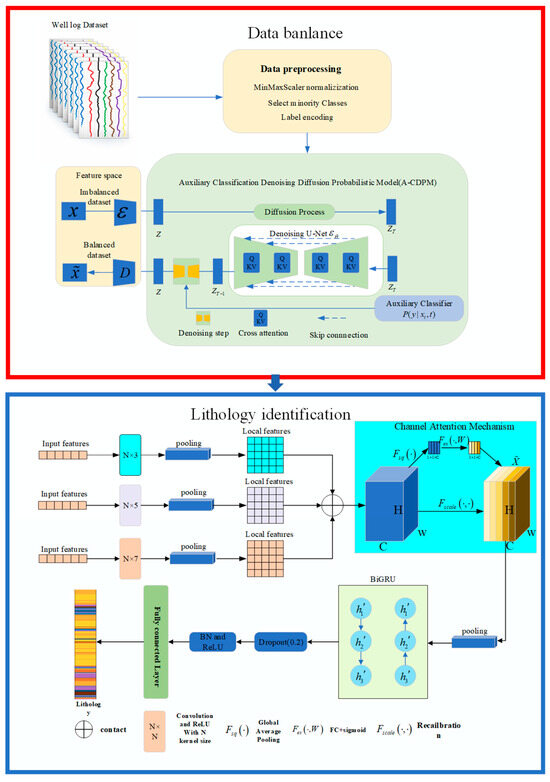
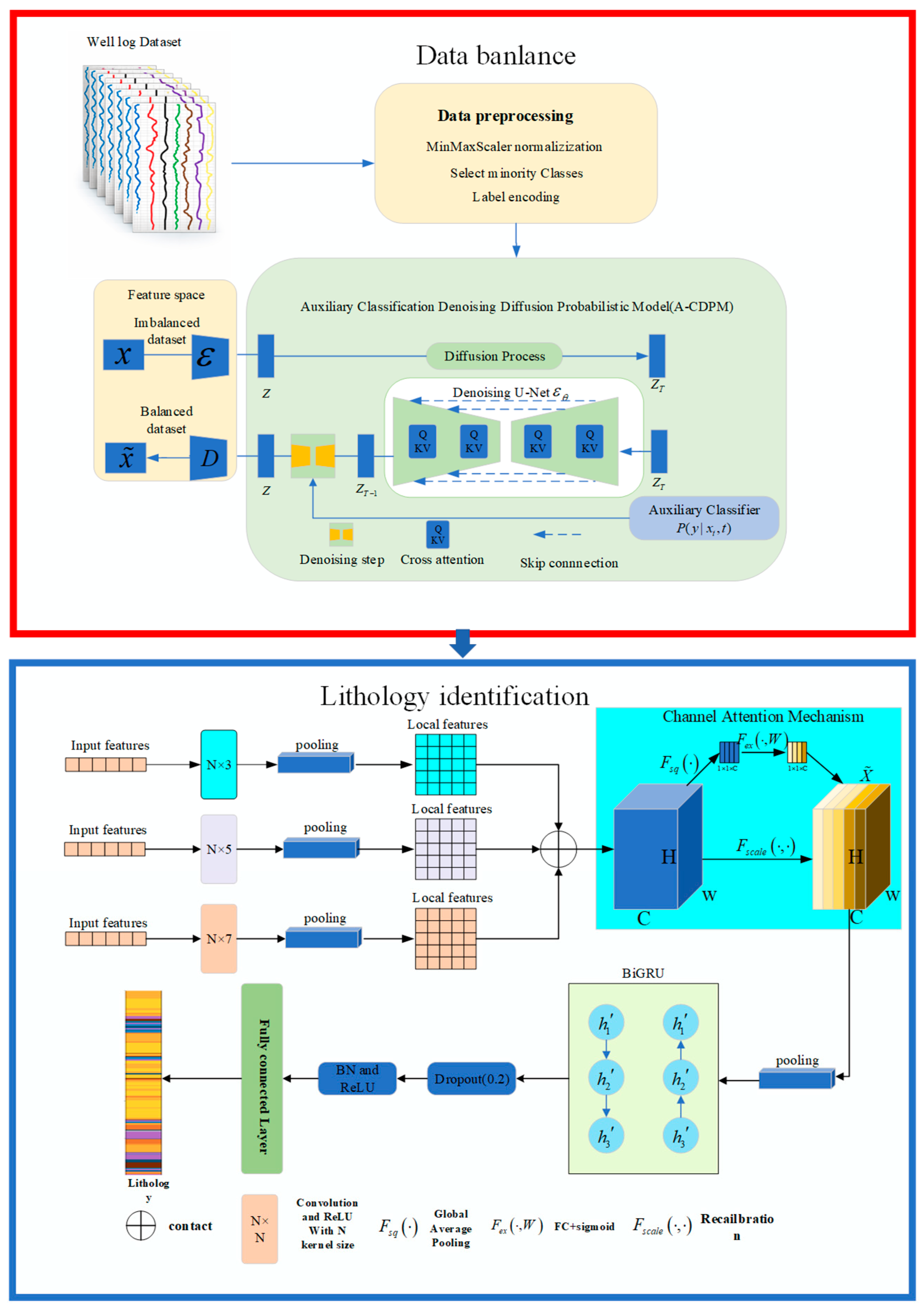
The workflow of the proposed A-CDPM-MSBG framework is illustrated in Figure 1, which mainly consists of two stages: data balancing and lithology identification. In the data balancing stage, A-CDPM is employed to generate well-log samples for minority classes, thereby alleviating data imbalance. In the lithology identification stage, a multi-scale convolutional network incorporating a channel attention mechanism is used to identify lithology.

Figure 1. The workflow of the (A-CDPM-MSBG). Data balancing addresses how to balance imbalanced datasets, while lithology identification explains how the network recognizes lithology.

2.1. Dataset Preparation and Description

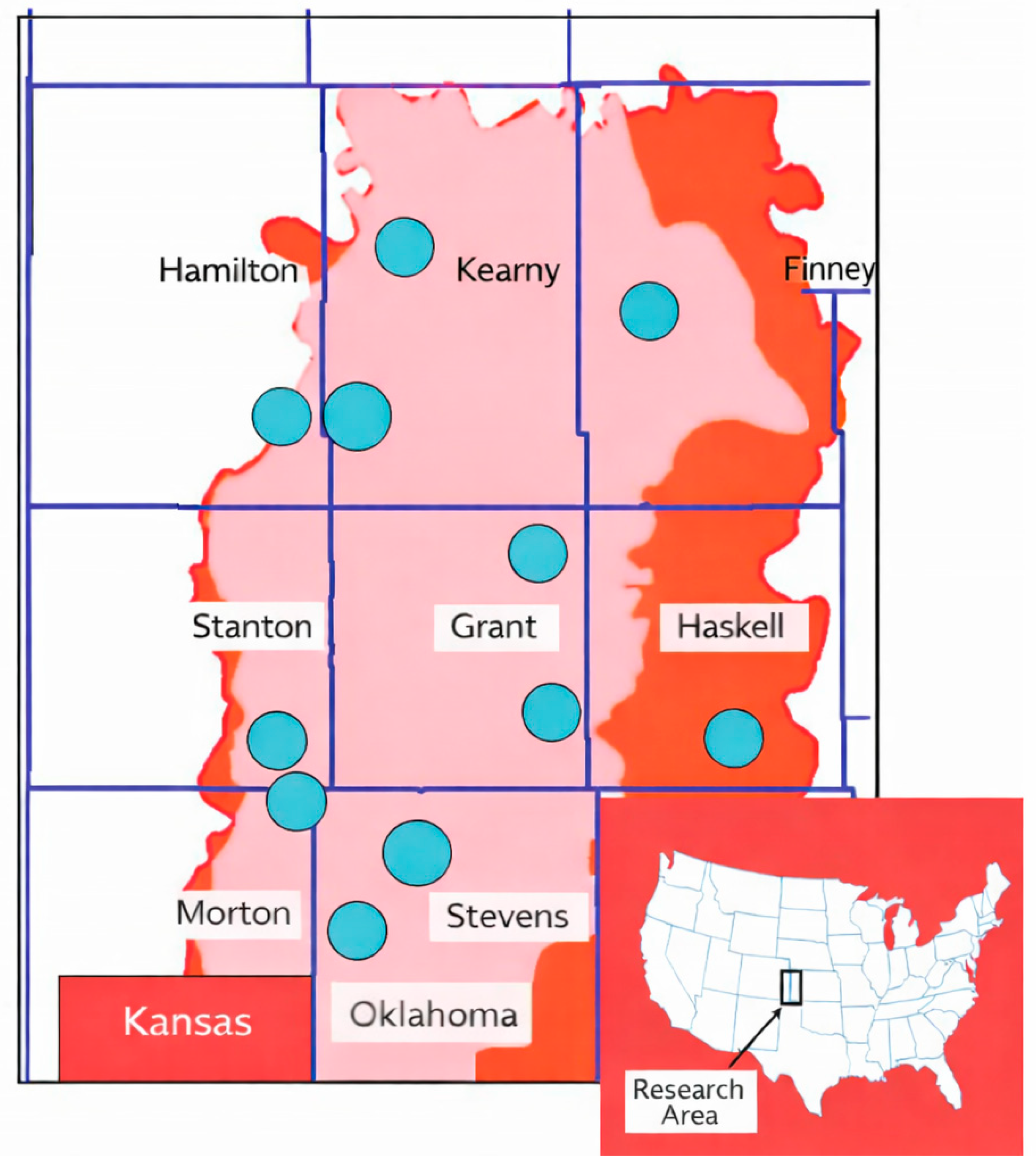
The study area of this experiment is located in the Hugoton and Panoma oil fields, situated in the southwestern part of Kansas and the northwestern part of Oklahoma, USA [34]. This region is one of the largest oil and gas fields in North America, with a total natural gas production of 9.63 × 10⁸ m³.

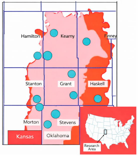
The experimental dataset is derived from core sample analysis of twelve wells in the region: SHRIMPLIN, ALEXANDER D, SHANKLE, LUKE G U, KIMZEY A, CROSS H, CATTLE NOLAN, Recruit F9, NEWBY, CHURCHMAN BIBLE, STUART, and CRAWFORD. The locations of the twelve wells are shown in Figure 2. The dataset includes well log data with a sampling interval of 0.5 m. The features of the well log data include natural gamma (GR), photoelectric factor (PE), deep resistivity (ILD), neutron density porosity (DeltaPHI), and average neutron density porosity (PHIND). Geological constraint variables include marine and non-marine indices (NM_M) and relative positions (RELPOS).

Figure 2. The locations of 12 oil wells in the Hugoton and Panoma oil fields of the study area [34].

2.2. Well Log Data Balancing Method

The input format of the well log data for the diffusion model is represented as (batch_size, num_channels, sequence_length), where batch_size refers to the number of samples in a batch, num_channels represents the number of well log channels, indicating the different well log features, and sequence_length refers to the number of sampling data points.

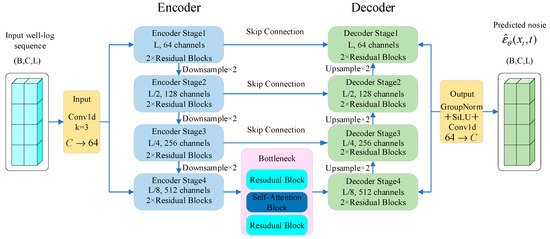
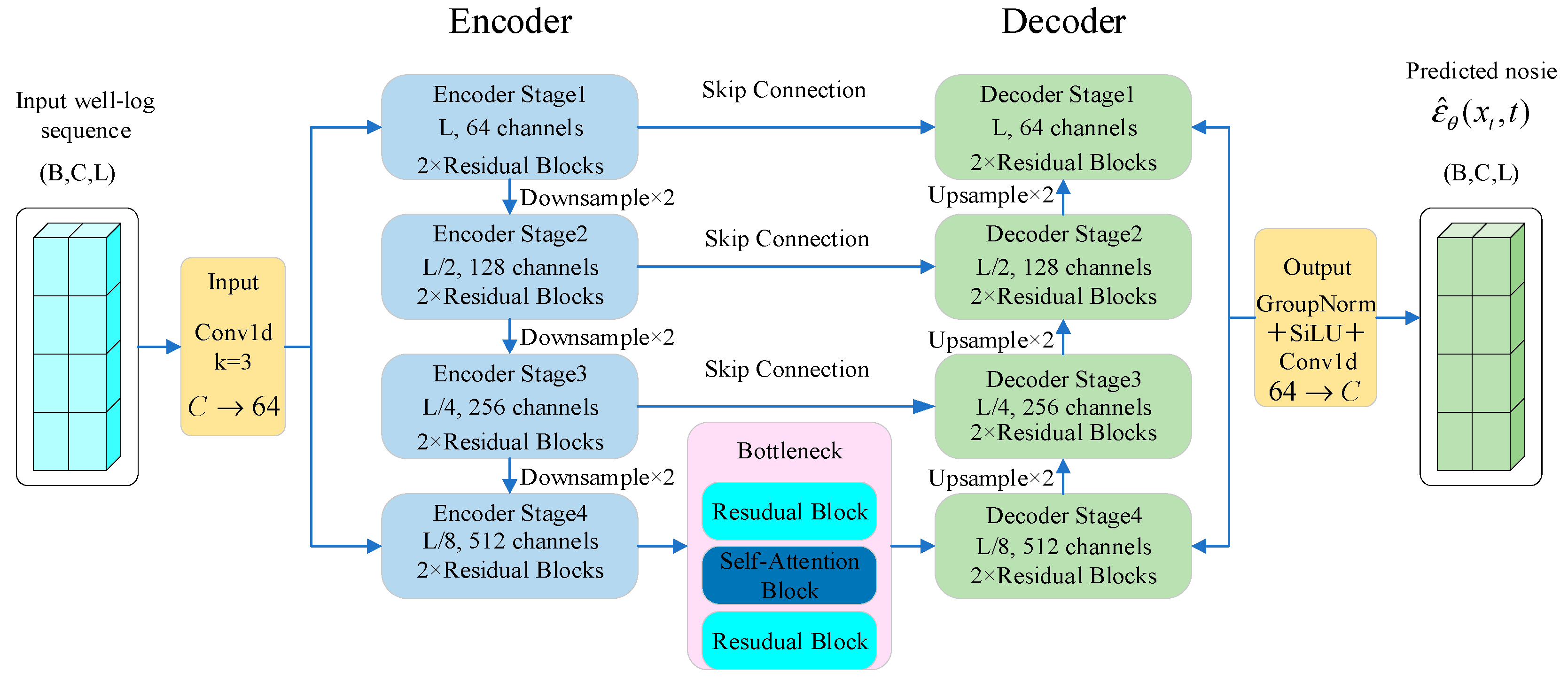
The model proposed in this paper, based on the auxiliary classifier and DDPM, consists of two main stages: the diffusion stage and the sampling generation stage. In the diffusion stage, noise is gradually injected into the well log data through a controlled noise-adding process, which corrupts the data in a stepwise manner, allowing the neural network to learn from it. The backbone network of the diffusion model typically uses MLP (Multilayer Perceptron) or U-net [35]. Among these, U-net is preferred for its encoder–decoder structure and skip connections, which make it highly suitable for handling one-dimensional sequential data, such as well log data. The 1D-Unet predicts the noise distribution at each diffusion step, guiding the data generation during the sampling process. Additionally, an auxiliary classifier is trained in the diffusion stage to help the network generate correct lithology samples during the sampling process. The classifier assists in maintaining category consistency, ensuring more accurate sample generation. The structure of the 1D-Unet network is shown in Figure 3. The input tensor is formatted as $\left(B,C,L\right)$, where $B$, $C$, and $L$ denote the batch size, the number of input well-log channels, and the sequence length, respectively. As shown in Figure 3, the 1D U-Net backbone adopts an encoder–decoder architecture with skip connections to extract and reconstruct multi-scale sequential features. The input projection layer maps the input channels to 64 feature channels using a 1D convolution with a kernel size of 3. The encoder consists of four stages with channel sizes of 64, 128, 256, and 512, corresponding to channel multipliers of [1, 2, 4, 8]. Each stage contains two residual blocks, and down-sampling with a factor of 2 is performed between consecutive stages. The bottleneck contains two residual blocks with one self-attention block inserted between them. The decoder mirrors the encoder and progressively restores the sequence resolution through up-sampling. GroupNorm and SiLU activation are used in the output head, and the time embedding dimension is set to 256.

Figure 3. Architecture of the 1D U-Net backbone. The network adopts an encoder–decoder structure with skip connections. The encoder and decoder contain four stages with channel multipliers of [1, 2, 4, 8], and each stage includes two residual blocks. A self-attention block is inserted at the bottleneck.

Diffusion Process:

The diffusion stage is a Markov chain that maps $x_0$ to $x_t$, progressively adding noise to the well-log data over $T$ time steps. This process can be represented as:

$$x_t=\sqrt{1-{\beta }_t}{x}_{t-1}+\sqrt{{\beta }_t}{\epsilon }_{t-1}$$

(1)

where $x_t$ represents the state of the well-log data at time step $t$, ${\beta }_t$ is the noise scaling factor, and ${\epsilon }_{t-1}$ is Gaussian noise sampled from a normal distribution. The noisy well-log data $x_t$ and time step $t$ are then input into the 1D U-Net network to predict the noise at each diffusion step.

To help the model distinguish different diffusion states, the time step $t$ is encoded using sine and cosine positional encoding:

$$T^{(2i)}=\sin \left({\displaystyle \frac{t}{{10000}^{\raisebox{1ex}{$2i$}\!\left/ \!\raisebox{-1ex}{$d$}\right.}}}\right)$$

(2)

$$T^{(2i+1)}=\cos \left({\displaystyle \frac{t}{{10000}^{\raisebox{1ex}{$2i$}\!\left/ \!\raisebox{-1ex}{$d$}\right.}}}\right)$$

(3)

where $2i$ and $2i+1$ denote the even and odd positions in the positional encoding, respectively, and $d$ represents the model dimension. The model is trained by minimizing the noise prediction error. The loss function can be formulated as follows:

$$\mathcal{L}=E{x}_0,t,{\epsilon }_t\left[{||{\epsilon }_{\theta }\left(x_t,t\right)-{\epsilon }_t||}^2\right]$$

(4)

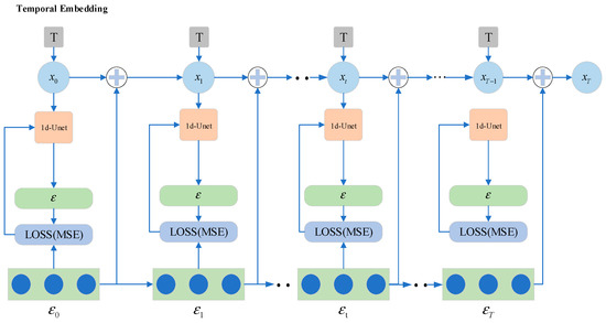
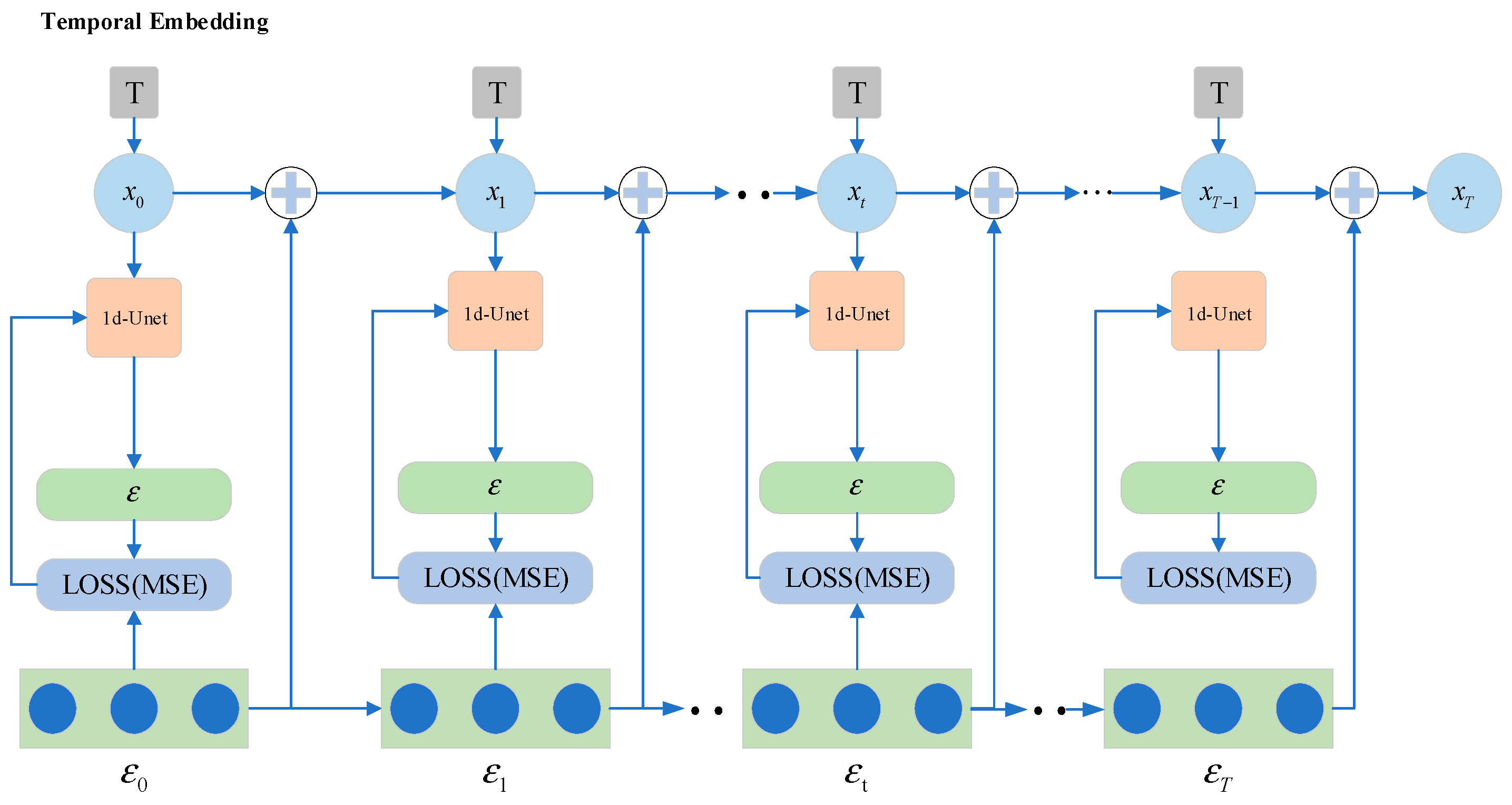
where $x_0$ represents the original clean data, $x_t$ represents the noisy data at time step t, and ${\epsilon }_t$ is the noise. The model predicts the noise ${\epsilon }_{\theta }\left(x_t,t\right)$ from the noisy data $x_t$ and compares it with the actual noise ${\epsilon }_t$ using the mean squared error (MSE) loss function. The diffusion process is shown in Figure 4.

Figure 4. Diffusion process. From left to right, $x_0$ is gradually transformed into $x_t$ by adding noise according to Equation (1). From bottom to top, the 1D U-Net is applied at each diffusion step to predict the noise distribution $\epsilon$, thereby guiding the sampling process. The loss is computed using the mean squared error (MSE) to ensure that the generated data align with the true data distribution, and the network parameters are updated accordingly.

Sampling Process:

The auxiliary classifier estimates the conditional probability distribution $p_{\varphi }(y\mid x_t,t)$ from the noisy data $x_t$ and the time variable $t$:

$$p_{\varphi }\left(y|x_t,t\right)=soft\max \left(f_{\varphi }\left(x_t,t\right)\right)$$

(5)

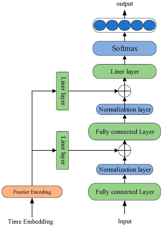
The architecture of the auxiliary classifier is shown in Figure 5. The resulting conditional probability gradient guides the reverse sampling process, encouraging the generated samples to match the target class label. The DDPM reverse process is expressed as follows:

$$x_{t-1}={\displaystyle \frac{1}{\sqrt{{\alpha }_t}}}(x_t-{\displaystyle \frac{1-{\alpha }_t}{\sqrt{1-\overline{{\alpha }_t}}}}{\epsilon }_{\theta }(x_t,t))+{\delta }_{t}z,z~\mathcal{N}(0,I)$$

(6)

$${\alpha }_t=1-{\beta }_t$$

(7)

where ${\epsilon }_{\theta }\left(x_t,t\right)$ denotes the predicted noise, and $z\sim \mathcal{N}(0,I)$ is a random noise term used to maintain sampling variability.

Figure 5. Architecture of the Auxiliary Classifier.

In classifier-guided diffusion sampling, the classifier gradient is used to guide the reverse denoising process toward the target class. According to Bayes’ rule, the conditional score can be decomposed as:

$${\nabla }_{x_t}\log p(x_t\mid y,t)={\nabla }_{x_t}\log p(x_t|t)+{\nabla }_{x_t}\log p_{\varphi }(y\mid x_t,t)$$

(8)

Under the $\epsilon -$ parameterization of DDPM, the unconditional score is related to the predicted noise by:

$${\nabla }_{x_t}\log p(x_t|t)\approx -{\displaystyle \frac{{ϵ}_{\theta }(x_t,t)}{\sqrt{1-{\overline{\alpha }}_t}}}$$

(9)

Substituting Equation (9) into Equation (8) gives:

$${\nabla }_{x_t}\log p(x_t|y,t)\approx -{\displaystyle \frac{{ϵ}_{\theta }(x_t,t)}{\sqrt{1-{\overline{\alpha }}_t}}}+{\nabla }_{x_t}\log p_{\varphi }(y|x_t,t)$$

(10)

Rewriting the conditional score in terms of a guided noise prediction ${\widehat{\epsilon }}_{\theta }(x_t,t,y)$ gives:

$${\nabla }_{x_t}\log p(x_t|y,t)\approx -{\displaystyle \frac{{\widehat{ϵ}}_{\theta }(x_t,t,y)}{\sqrt{1-{\overline{\alpha }}_t}}}$$

(11)

By comparing Equation (10) and Equation (11), the classifier-guided noise prediction is obtained as:

$${\widehat{\epsilon }}_{\theta }(x_t,t,y)={\epsilon }_{\theta }(x_t,t)-\lambda \sqrt{1-{\overline{\alpha }}_t}\nabla x_t\log p_{\varphi }(y|x_t,t)$$

(12)

where $\lambda$ is a tunable hyperparameter controlling the strength of the classifier guidance. The negative sign before the classifier-gradient term results from the conversion between the score function and the $\epsilon$-parameterized noise prediction, rather than from reversing the guidance direction. This formulation guides the generated samples toward the target lithology class while preserving the stochasticity of the reverse diffusion process.

The reverse sampling process is then updated as:

$$x_{t-1}={\displaystyle \frac{1}{\sqrt{{\alpha }_t}}}\left(x_t-{\displaystyle \frac{1-{\alpha }_t}{\sqrt{1-\overline{{\alpha }_t}}}}{\widehat{\epsilon }}_{\theta }\left(x_t,t,y\right)\right)+{\delta }_{t}z$$

(13)

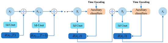
This process continues until the final sample $x_0$ is generated, which represents the denoised version of the initial noisy sample. The classifier-guided sampling process is illustrated in Figure 6.

Figure 6. Sampling Process Guided by an Auxiliary Classifier: From left to right, the noise predicted by DDPM is refined under the guidance of the auxiliary classifier, and the well-log data are then iteratively updated from $x_T$ to $x_0$.

The process of generating well-log data using the A-CDPM is shown in Algorithm 1. The training procedure of the auxiliary classifier is presented in Algorithm 2.

Algorithm 1: Process for Generating Well log Data with the A-CDPM

Input: Imbalanced well-log dataset $D_{imb}={\{(x_i,y_i)\}}_{i=1}^N$, Minority class set $C_{\min }$, Output: Balanced dataset $D_{bal}$ 1: $D_{bal}\leftarrow D_{imb}$ 2: Train the denoising network ${\epsilon }_{\theta }$ and the auxiliary classifier $p_{\varphi }$ separately. 3: for each class c in $C_{\min }$ do 4: Compute the required number of generated samples Mc 5:   for i = 1 to Mc do 6:  Sample $x_T\sim \mathcal{N}(0,I)$ 7:  for t = T down to 1 do 8:    Compute guided the noise estimate ${\widehat{\epsilon }}_{\theta }(x_t,t,y)$ according to Equation (12) 9:    Update $x_{t-1}$ from $x_t$ according to Equation (13) 10:   end for 11:   $D_{bal}\leftarrow D_{bal}\cup \{(x_0,c)\}$ 12: end for 13: end for 14: return $D_{bal}$

Algorithm 2: Auxiliary classifier training algorithm

1: Input: Noisy well-log data $x_t$, Lithology labels, $y$ timestep $t$, Model parameters $\varphi$ number of iterations $N$, 2: Output: trained auxiliary classifier $p_{\varphi }\left(y∣x_t,t\right)$, 3: for i = 1 to N 4:   Convert the time vector $t$ into a time encoding $T$ 5:   Pass T through multiple linear layers to obtain intermediate features $T_1,T_2\dots T_m$ 6:   Feed $T_1,T_2\dots T_m$ and the data $x_t$ into the model to compute the output $p_{\varphi }(y\mid x_t,t)$ 7:   Compute the cross-entropy loss based on the predicted results and the true labels. 8:   Update the network parameters using an optimizer according to the loss $\mathcal{L}$ 9: end for 10: return $p_{\varphi }(y\mid x_t,t)$

2.3. Lithology Identification Framework

Based on the lithology identification model, traditional lithology identification methods face challenges such as insufficient feature extraction and information loss when handling complex formation data. To address these issues, this paper proposes a lithology identification model that integrates multi-scale convolution, channel attention mechanisms, and bidirectional GRU.

2.3.1. Multi-Scale Convolutional Neural Network

In conventional convolutional neural networks for logging feature extraction, fixed-size convolutional kernels are typically employed [36]. However, such fixed-scale designs exhibit limited capacity in capturing geological features at varying spatial scales, particularly in structurally complex stratigraphic environments. To overcome this limitation, we propose a multi-scale convolutional module comprising parallel branches with different kernel sizes, specifically (kernel sizes = 3), (kernel sizes = 5), and (kernel sizes = 7). This architecture enables the simultaneous extraction of fine-grained local details and broad contextual representations, thereby enhancing the model’s ability to perceive multi-scale lithological patterns. In the present study, the 3-5-7 combination was adopted as a commonly used empirical multi-scale configuration for one-dimensional well-log sequences, aiming to capture local fluctuations, intermediate lithological transitions, and relatively broader contextual dependencies simultaneously. This setting was used to balance feature diversity, model complexity, and training stability.

2.3.2. Improved Channel Attention Mechanism Method

The attention mechanism can be categorized into spatial domain, channel domain, layer domain, hybrid domain, and temporal domain based on the different attention focus areas [37]. To account for the complexity of time and the compatibility with multi-scale convolutions, a channel-domain-based compression and excitation network (SE Net) [38] is employed to implement the attention mechanism. This module learns channel-wise weights in an end-to-end manner during model training.

After feature extraction, average pooling and max pooling are applied along the depth dimension to obtain compact channel descriptors, as follows:

$$\left\{\begin{array}{l}{z}_{avg}^c={\displaystyle \frac{1}{T}}{\displaystyle \sum _{t=1}^T{X}_t^c}\hfill \\ z_{max}^c=\underset{t\in [1,T]}{\max }{X}_t^c\hfill \end{array}\right.$$

(14)

where $X_t^c$ denotes the feature value of channel $c$ at depth index $t$, T is the sequence length, and $z_{avg}^c$ and $Z_{max}^c$ represent the average and maximum responses of channel c, respectively. The two channel descriptors are concatenated and passed through two fully connected layers and a sigmoid activation function to generate the channel-wise attention weight:

$$s_c=\sigma \left(W_2\cdot \delta \left(W_1\cdot \left[z_{avg}^c;z_{max}^c\right]+b_1\right)+b_2\right)$$

(15)

where $W_1$ and $W_2$ are trainable weight matrices, $b_1$ and $b_2$ are bias terms, $\delta$ represents the activation function, and the reduction ratio is set to 8. The original feature maps are then recalibrated by multiplying them with the learned channel weights:

The channel weight $s_c$ is multiplied by the channel features, completing the enhancement of lithological features and channel strength. The calculation formula is as follows:

$$y_t^c=X_t^c\cdot s_c$$

(16)

where $y_t^c$ represents the recalibrated feature of channel $c$ at depth index $t$. Through this process, informative feature channels are enhanced, while less relevant channel responses are suppressed.

2.3.3. BiGRU Model Algorithm

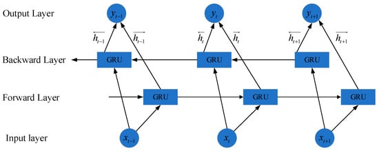
The BiGRU model extends the standard GRU by introducing both forward and backward recurrent layers. This structure enables the model to capture contextual information from both previous and subsequent well-log sequences, thereby improving sequential feature representation for lithology classification. The structure of the BiGRU model is illustrated in Figure 7.

Figure 7. The structure diagram of the BiGRU (Bidirectional GRU) unit.

At each time step $t$, the forward GRU processes the sequence from time step 1 to $T$, while the backward GRU processes the sequence in the reverse direction. The hidden states of the two directions are computed as follows:

$$\overrightarrow{h_t}=GRU(x_t,\overrightarrow{h_{t-1}})$$

(17)

$$\overleftarrow{h_t}=GRU(x_t,\overleftarrow{h_{t-1}})$$

(18)

The final hidden representation is obtained by concatenating the forward and backward hidden states:

$$h_t=[{\overrightarrow{h}}_t;{\overleftarrow{h}}_t]$$

(19)

where ${\overrightarrow{h}}_t$ and ${\overleftarrow{h}}_t$ denote the forward and backward hidden states at time step $t$, respectively. This bidirectional structure allows the model to integrate contextual dependencies in both directions and provides richer sequential features for subsequent lithology classification.

3. Results

3.1. Dataset Analysis and Preprocessing

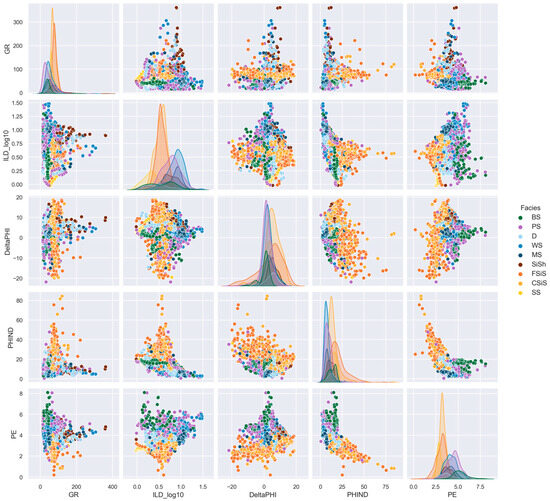
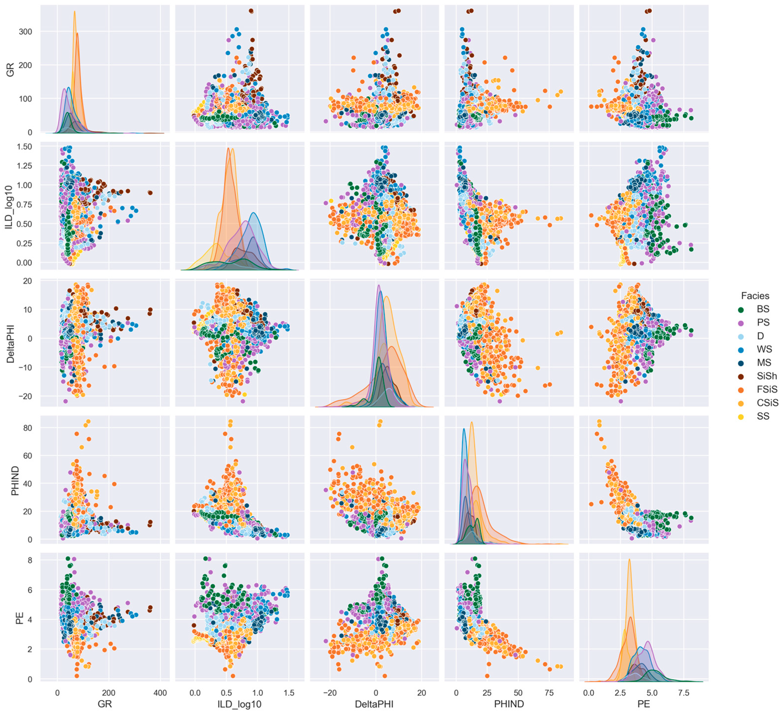
To illustrate the relationship between well-log features and lithology classes, Figure 8 presents cross-plots that visualize the distributions of different well-log features. Table 1 provides a summary of the relevant information for each lithology class. As shown in Table 1, the dataset exhibits significant class imbalance among lithology samples. Figure 8 also indicates that different lithologies have varying sensitivity to the well-log parameters. However, considerable overlap and unclear boundaries remain between different lithology groups. This overlap complicates the interpretation and discrimination of individual lithologies, increasing the difficulty of lithology identification.

Figure 8. The cross-plots of the logging curves for nine lithologies in the Hugoton and Panoma oilfield.

Table 1. Lithological information.

Lithology	Label	Number	Sample Size	Proportion
Nonmarine sandstone	SS	0	279	6.87%
Nonmarine coarse siltstone	CSiS	1	897	22.08%
Nonmarine fine siltstone	FSiS	2	769	18.93%
Marine siltstone and shale	SiSh	3	249	6.13%
Mudstone	MS	4	266	6.55%
Wackestone	WS	5	589	14.50%
Dolomite	D	6	124	3.06%
Packstone–grainstone	PS	7	710	17.48%
Phylloid-algal bafflestone	BS	8	179	4.41%

To improve the stability and convergence speed of model training, reduce the scale differences among different well-log features, and enhance the quality of the generated data as well as the classification performance, we first applied min-max normalization to the data. This operation linearly scales each feature to the range of [0, 1], as shown in Equation (20)

$$y={\displaystyle \frac{x-x_{\min }}{x_{\max }-x_{\min }}}$$

(20)

where $x$ is the original well-log data, $x_{min}$ is the minimum value of the data, $x_{max}$ is the maximum value of the data, and $y$ represents the normalized data.

3.2. Model Evaluation Metrics

In imbalanced datasets, we evaluate the effectiveness of the lithology classification model using accuracy, precision, recall, and F1 score.

$$A\mathrm{ccurary}={\displaystyle \frac{TP+TN}{TP+TN+FP+FN}}$$

(21)

$$\mathrm{Re}call={\displaystyle \frac{TP}{TP+TN}}$$

(22)

$$\mathrm{Pr}ecision={\displaystyle \frac{TP}{TP+FP}}$$

(23)

$$F1=2\cdot {\displaystyle \frac{precision\cdot recall}{precision+recall}}$$

(24)

Here, TP refers to the number of correctly identified lithology samples, FN refers to the number of incorrectly predicted lithology samples, FP refers to the lithology samples incorrectly predicted as the correct class, and TN refers to the lithology samples incorrectly predicted as the negative class.

3.3. A-CDPM Training Process

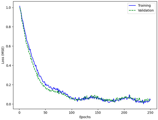
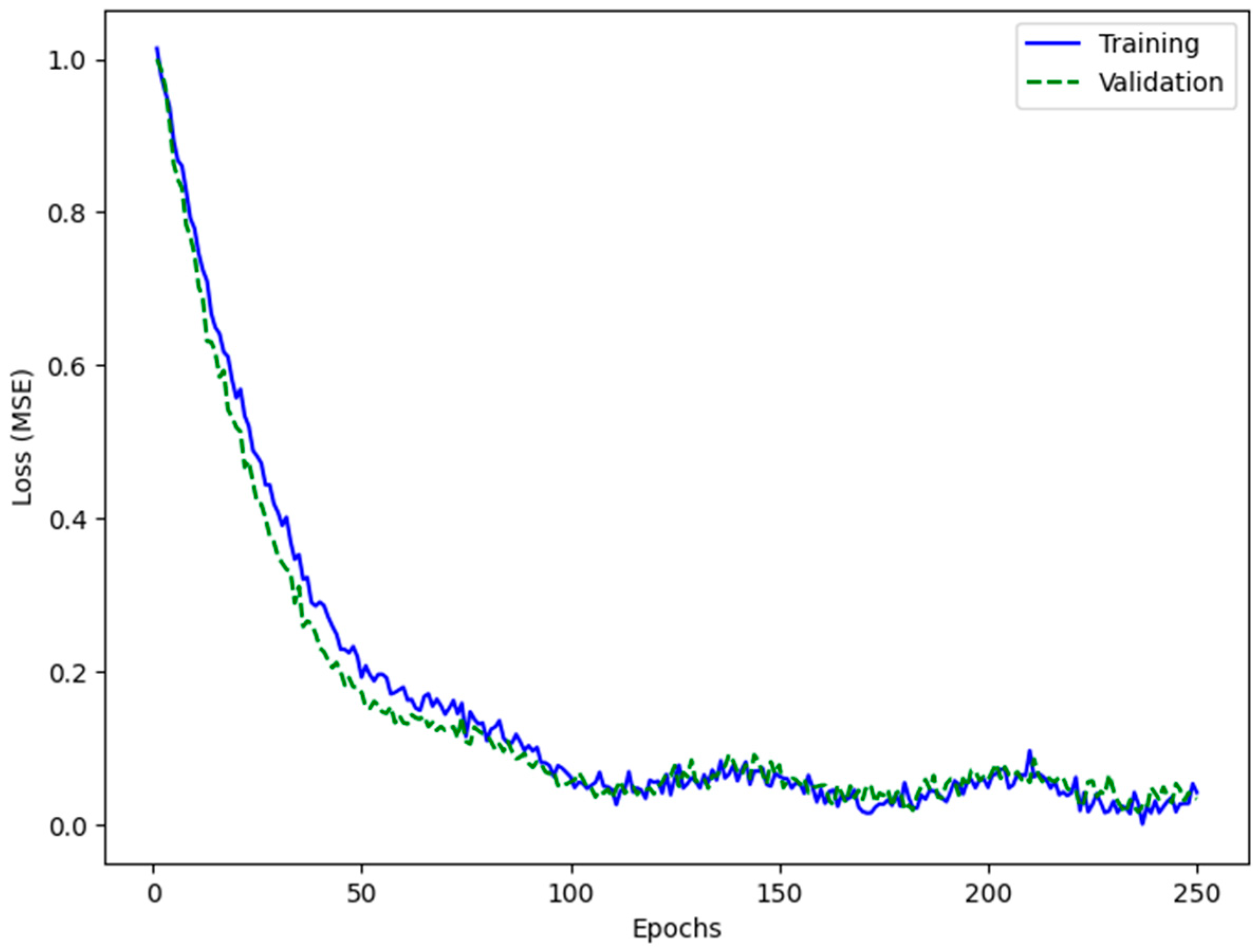
The experimental process of A-CDPM is as follows: The training and validation sets are divided in an 8:2 ratio. AdamW is used as the optimizer for A-CDPM. AdamW is a variant of the Adam optimizer with the addition of a weight decay term. The learning rate is set to 1 × 10⁻⁴, and the weight decay is set to 0.01, with default parameters and a cosine annealing learning rate schedule. The batch size is 32, and the training runs for 250 epochs, with a dropout rate of 0.2. Figure 9 shows the change in the loss function during the training process.

Figure 9. The training and validation loss curves during the A-CDPM training process.

As shown in Figure 9, both the training loss and validation loss decreased rapidly in the initial stage and then gradually reached a stable state. After about 100 epochs, both curves fluctuated slightly at a low level. Moreover, the validation loss remained close to the training loss throughout the training process, indicating that the model achieved good convergence and did not exhibit obvious overfitting.

3.4. Evaluation of Generated Data Quality

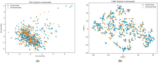
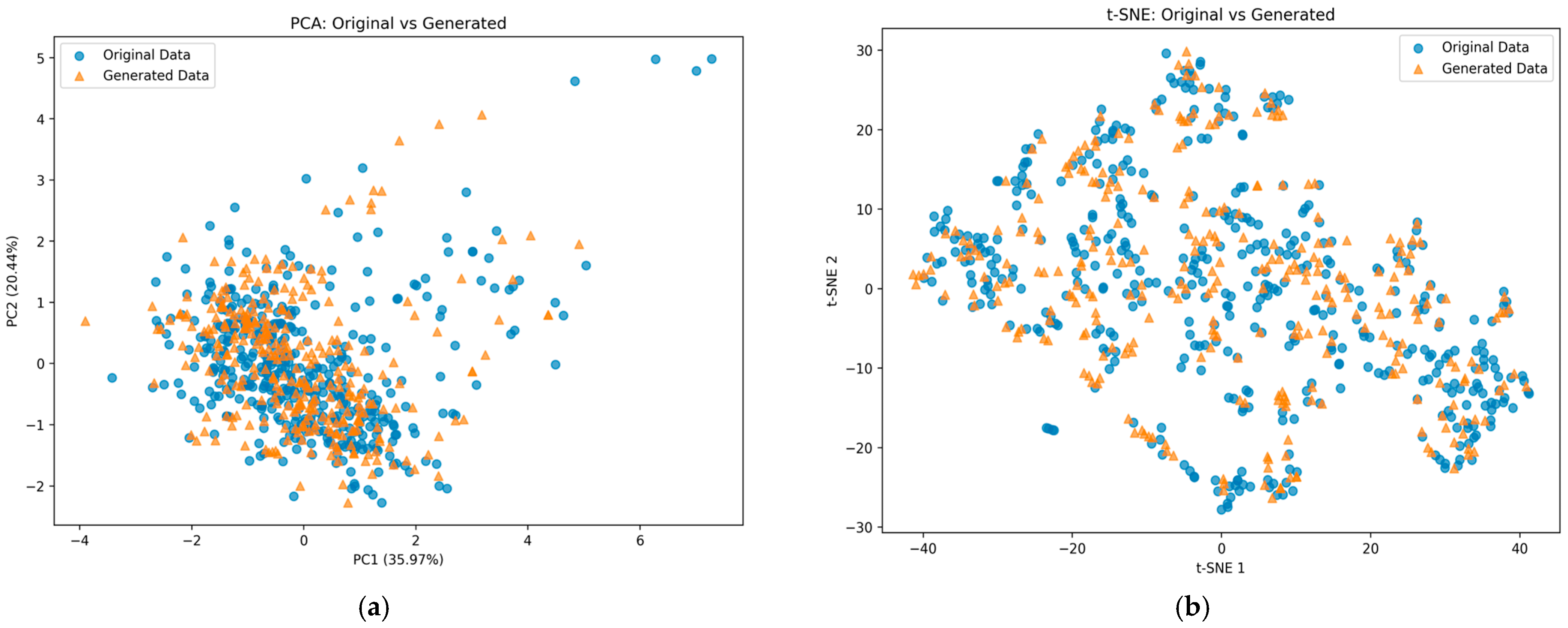
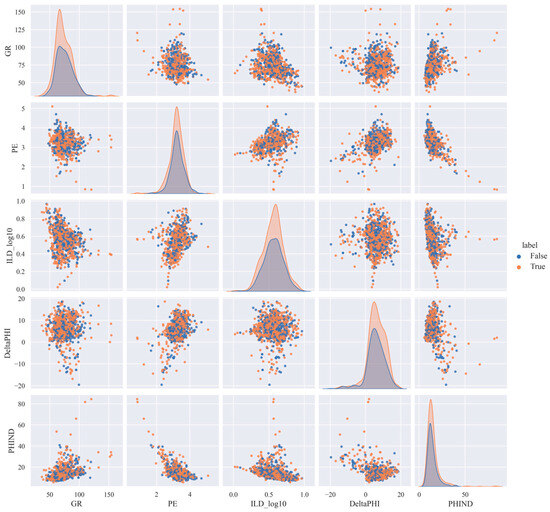
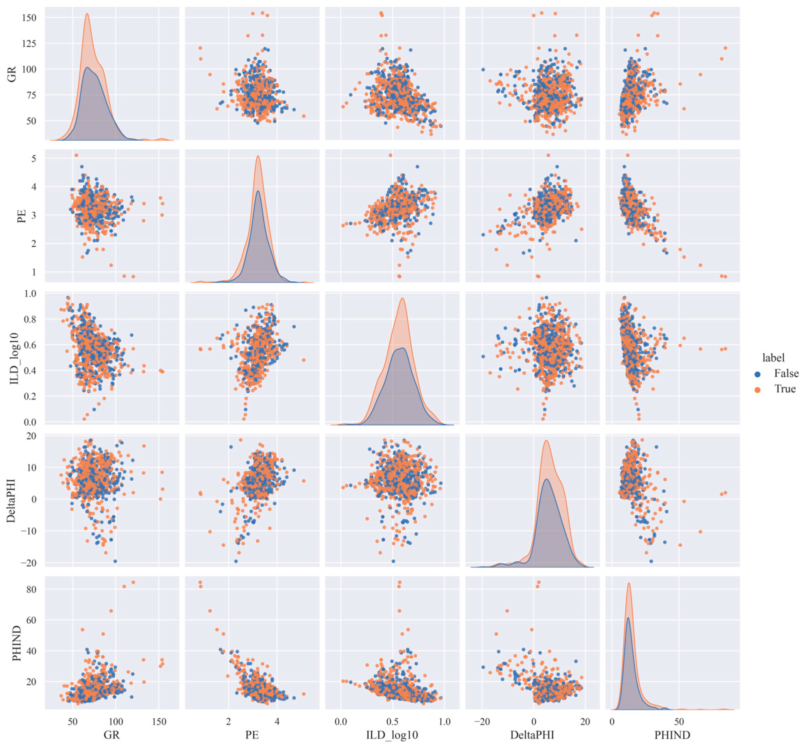
To visually evaluate the quality of the well-log-generated data, we compared the generated and original samples from two perspectives: low-dimensional distribution structure and multi-feature relationships. PCA and t-SNE were employed to assess the similarity between the two datasets, where PCA reflects the preservation of the global distribution structure and t-SNE reveals the consistency of local neighborhood patterns. In addition, pairwise feature distributions were examined to compare the joint relationships among multiple well-log variables. As shown in Figure 10, the generated and original data exhibit substantial overlap in both PCA and t-SNE spaces, indicating that the generated samples preserve not only the global distribution characteristics of the original data but also their local manifold structure. Figure 11 further shows that the generated data are generally consistent with the original data in terms of marginal distributions and pairwise feature relationships, suggesting that the proposed method can effectively reproduce the main statistical characteristics of the well-log data.

Figure 10. Comparison of the distribution of generated data and original data in the reduced-dimensional space. (a) PCA plot comparing the distribution of the original and generated data. (b) t-SNE plot comparing the distribution of the original and generated data.

Figure 11. Shows the distribution of the generated data and the original data, where the original data is labeled as “True”, and the generated data is labeled as “False”.

3.5. Effectiveness Validation

To thoroughly validate the effectiveness of the proposed denoising diffusion model guided by auxiliary classification and the intelligent lithology recognition framework for classification accuracy on imbalanced datasets, multiple ablation and comparison experiments on the same dataset were designed to verify the results.

In the main experiment, the original dataset was first stratified into training, validation, and test sets with a ratio of 8:1:1. The validation and test sets retained their original real-sample distributions, while data augmentation was applied only to the training set. To alleviate class imbalance, minority lithologies in the training set were augmented to match the size of the largest class in the training set. The lithology-wise sample counts for the train/validation/test split and the augmented training set are reported in Table 2.

Table 2. Distribution of lithology samples in the training, validation, and test.

Lithology	Train	Validation	Test	Augmented Train
SS	223	28	28	718
CSiS	718	90	89	718
FSiS	615	77	77	718
SiSh	199	25	25	718
MS	213	27	26	718
WS	471	59	59	718
D	99	12	13	718
PS	568	71	71	718
BS	143	18	18	718

3.5.1. Comparison Experiment

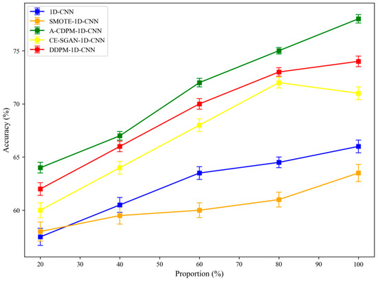
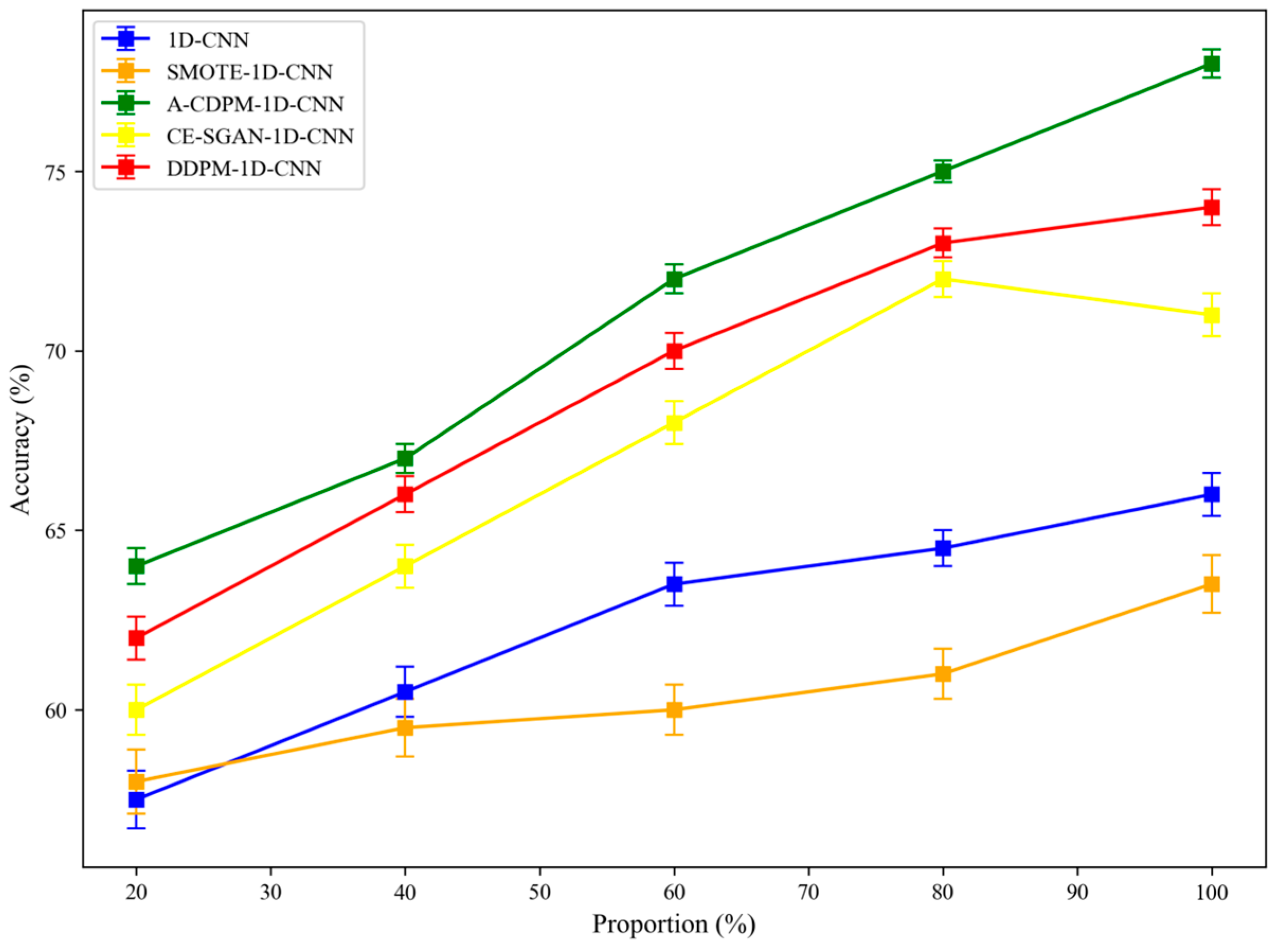
To evaluate the classification enhancement effect of A-CDPM compared to other data augmentation methods, datasets with different sampling ratios were used to simulate lithological imbalance. To account for the randomness in data sampling, each experiment was repeated ten times, and the results are reported as the mean with error bars to reflect variability, as shown in Figure 12.

Figure 12. The accuracy of different data augmentation models, with the extraction of varying proportions of data from the dataset to control the number of minority samples.

3.5.2. Ablation Experiment

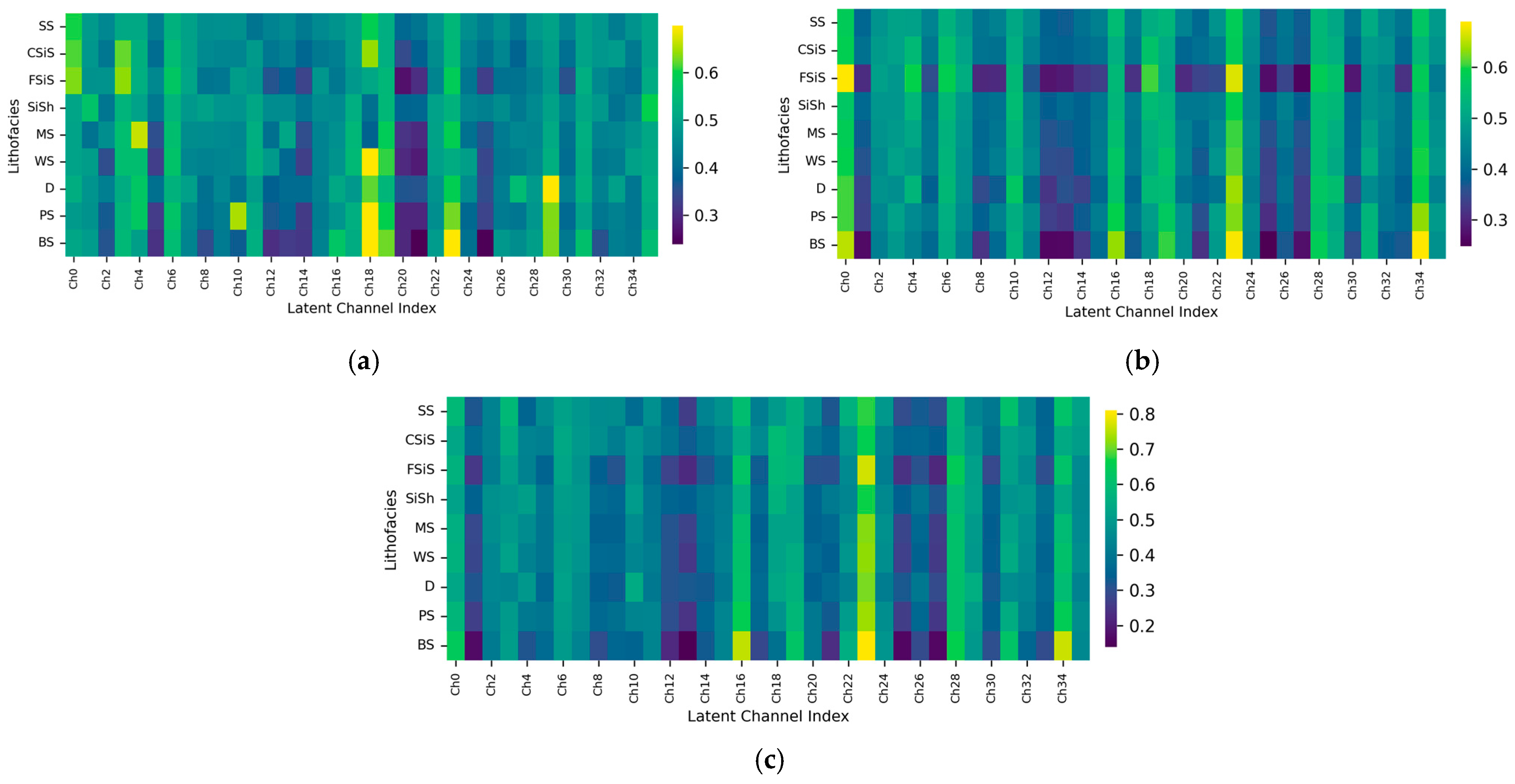
To verify the necessity of integrating average pooling and max pooling in the channel attention module, we compared three pooling strategies: average pooling only, max pooling only, and combined average-and-max pooling. Since the aim of this ablation study was to evaluate the contribution of the pooling strategy itself rather than the effect of diffusion-based data augmentation, the comparison was conducted on the original real dataset. All other network structures, training settings, and data splits were kept identical to ensure a fair comparison. Table 3 presents the results of the ablation study on different pooling strategies in the channel attention module. Figure 13 shows the distributions of channel attention weights across lithofacies under three pooling strategies.

Table 3. Ablation study of different pooling strategies in the channel attention module.

Model	Accuracy (%)	Precision (%)	Recall (%)	F1 Score (%)
Avg Pooling	74.05	66.15	66.75	63.28
Max Pooling	75.32	71.54	66.45	65.33
Avg Pooling + Max Pooling	80.13	79.27	78.34	78.90

Figure 13. Visualization of channel attention weight distributions across lithofacies under three pooling strategies. (a) Combination of Average Pooling and Max Pooling. (b) Max Pooling. (c) Average Pooling.

Table 3 shows the combined pooling strategy achieved the best performance on all evaluation metrics, with Accuracy, Precision, Recall, and F1 Score reaching 80.13%, 79.27%, 78.34%, and 78.90%, respectively. Compared with average pooling alone, the combined strategy improved Accuracy, Precision, Recall, and F1 Score by 6.08%, 13.12%, 11.59%, and 15.62%, respectively. Compared with max pooling alone, the corresponding improvements were 4.81%, 7.73%, 11.89%, and 13.57%. These results indicate that a single pooling strategy is insufficient to fully characterize the importance of different lithologic channels, whereas the combined pooling strategy provides a more effective channel representation and significantly improves lithology classification performance.

As shown in, compared with single pooling strategies, the combination of max pooling and average pooling exhibits a clearer and more stable channel-weight distribution pattern. While preserving inter-channel differences, this strategy presents a more continuous response structure, and the weight variations in different lithofacies across several key latent channels become more distinct and easier to differentiate. In addition, this strategy more stably highlights highly responsive channels while suppressing weakly responsive ones, thereby forming a more discriminative channel attention distribution.

To validate the contribution of each component in the proposed model to the recognition performance, we conducted ablation experiments, evaluating the effect of the A-CDPM data augmentation model, as well as the impact of multi-scale convolution, BiGRU, and the channel attention mechanism on lithology recognition performance. The results are presented in Table 4.

Table 4. Results of the ablation experiment using the Hugoton–Panoma dataset.

Model	Accuracy (%)	Precision (%)	Recall (%)	F1 Score (%)
MCNN	64.58	62.36	64.08	63.28
MCNN-BiGRU	64.64	64.82	64.46	64.64
A-CDPM-MCNN-BiGRU	76.68	75.67	74.38	74.99
MCNN-BiGRU-channel attention	80.13	79.27	78.34	78.80
A-CDPM-MCNN-BiGRU-channel attention	86.66	85.44	84.78	85.11

As shown in Table 4, the ablation results reveal clear differences in the contributions of individual modules to lithology identification performance. The baseline MCNN achieved an Accuracy, Precision, Recall, and F1 Score of 64.58%, 62.36%, 64.08%, and 63.28%, respectively. After introducing BiGRU, the performance improved only marginally, indicating that sequence modeling alone provides limited benefit under the current data conditions. In contrast, the incorporation of A-CDPM-based data augmentation led to a substantial improvement, with A-CDPM-MCNN-BiGRU achieving 76.68% Accuracy, 75.67% Precision, 74.38% Recall, and 74.99% F1 Score, demonstrating that diffusion-based augmentation effectively alleviates the impact of data imbalance. With the further introduction of the channel attention mechanism, the model performance was improved again. In particular, MCNN-BiGRU-channel attention achieved an Accuracy of 80.13%, highlighting the positive effect of channel recalibration on feature representation. The full model, A-CDPM-MCNN-BiGRU-channel attention, achieved the best overall performance, with Accuracy, Precision, Recall, and F1 Score reaching 86.66%, 85.44%, 84.78%, and 85.11%, respectively. These results indicate that A-CDPM-based augmentation and channel attention exhibit a clear complementary effect, jointly enhancing lithology identification performance in complex settings.

3.5.3. Comparison with Other Models

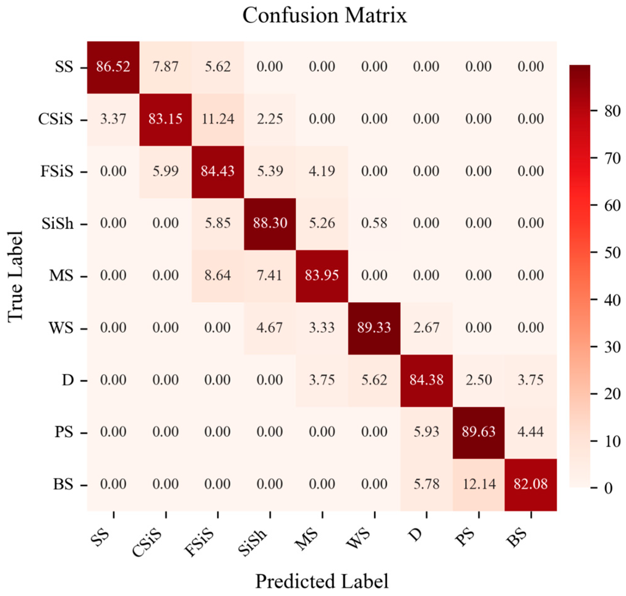
To validate the superiority of the method proposed in this paper, the proposed method was compared with other previous models on the same dataset. Figure 14 presents the confusion matrix for each lithology of the A-CDPM-MSBG model on the test set. The comparative results with other models are presented in Table 5.

Figure 14. Confusion matrix of A-CDPM-MSBG on the test set.

Table 5. Comparison of Lithology Identification using Different Models in Hugoton–Panoma.

Model	Accuracy (%)	Precision (%)	Recall (%)	F1 Score (%)
GDBT	56.64	58.10	51.45	54.56
XGBoost	57.71	60.06	57.71	59.04
RF	61.45	64.05	61.44	62.72
SVM	63.13	61.73	63.13	62.22
KNN	71.33	69.89	71.02	75.53
1D-CNN (Adagrad) [39]	74.58	74.93	75.57	74.25
1D-CNN (Adadelta) [39]	73.37	71.89	72.55	72.22
1D-CNN (Adamax) [39]	76.87	74.93	75.57	74.25
CE-SGAN [23]	79.88	78.93	80.62	84.56
LSTM [39]	62.59	60.85	61.66	66.26
RNN [39]	57.38	55.52	54.86	52.88
A-CDPM-MSBG (ours)	86.66	85.44	84.78	85.11

3.5.4. Comparison of Adjacent Blind Wells

To evaluate the model’s predictive capability in different regions, we designed the Blind Well Test. Specifically, the trained lithology recognition model was applied to data from adjacent wells that were not involved in the training or testing phases for lithology prediction. This method validates the model’s prediction accuracy on new wells and tests its generalization performance. We evaluated the proposed A-CDPM-MSBG model against other commonly used models. The experimental results of the adjacent blind well evaluation on the Hugoton–Panoma datasets are presented in Table 6.

Table 6. Blind Well Comparison Experiment Results.

Model	Accuracy (%)	Precision (%)	Recall (%)	F1 Score (%)
GDBT	58.66	56.48	58.72	56.18
RF [39]	61.45	64.05	61.44	62.72
SVM [39]	60.13	52.62	62.43	62.08
KNN [39]	63.73	65.66	64.73	64.69
1D-CNN (Adagrad) [39]	66.52	65.82	68.98	62.12
CE-SGAN [23]	68.83	64.72	69.22	63.91
MS-CGAN [24]	69.82	69.96	69.52	63.91
LSTM [39]	56.32	54.15	58.62	56.22
A-CDPM-MSBG (ours)	75.66	78.56	73.29	77.78

3.6. Visualization

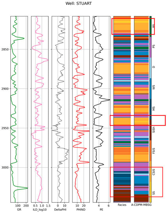
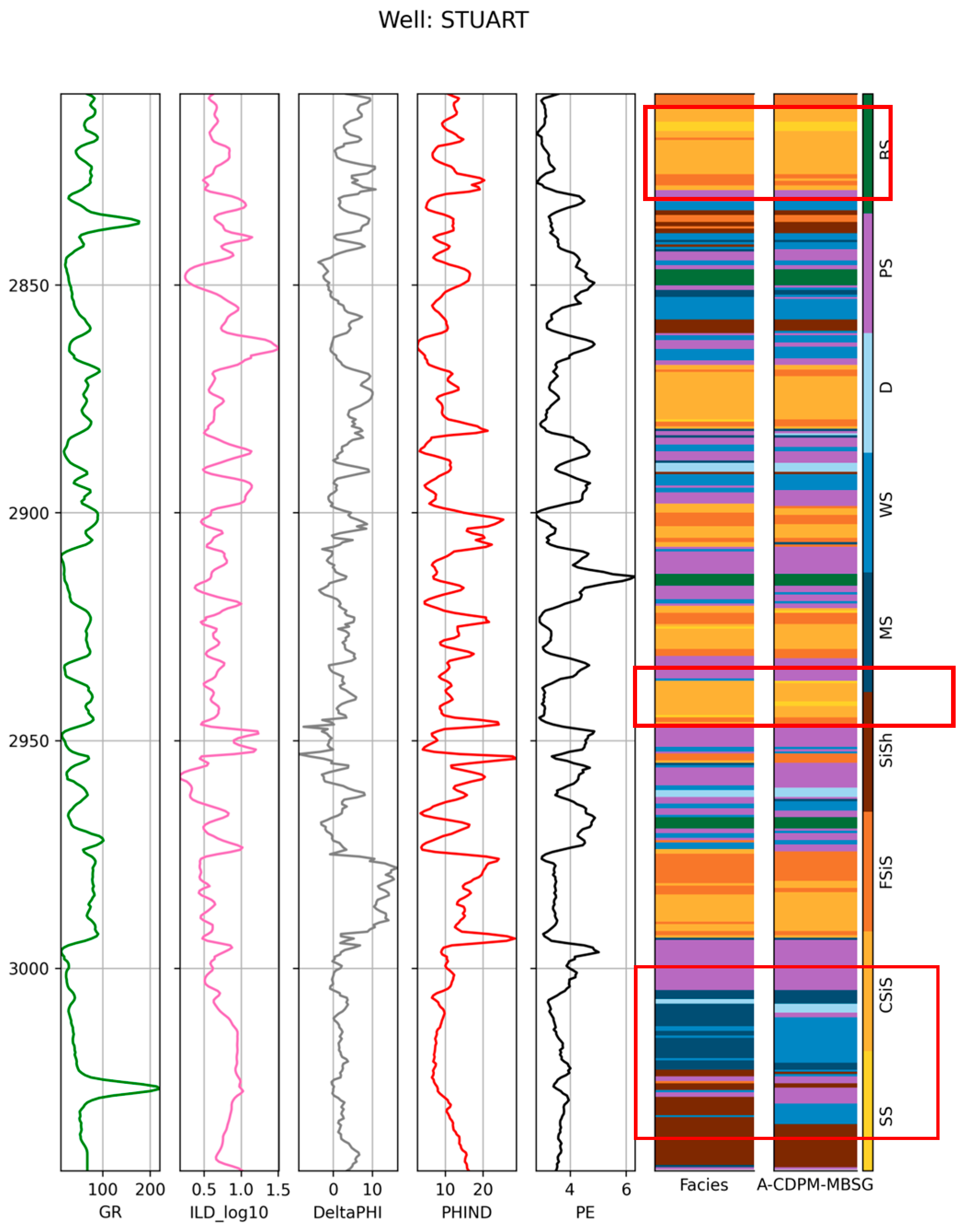
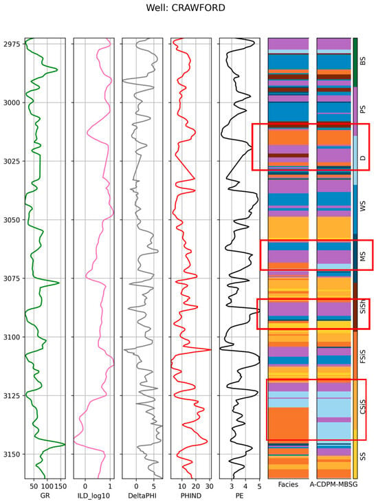
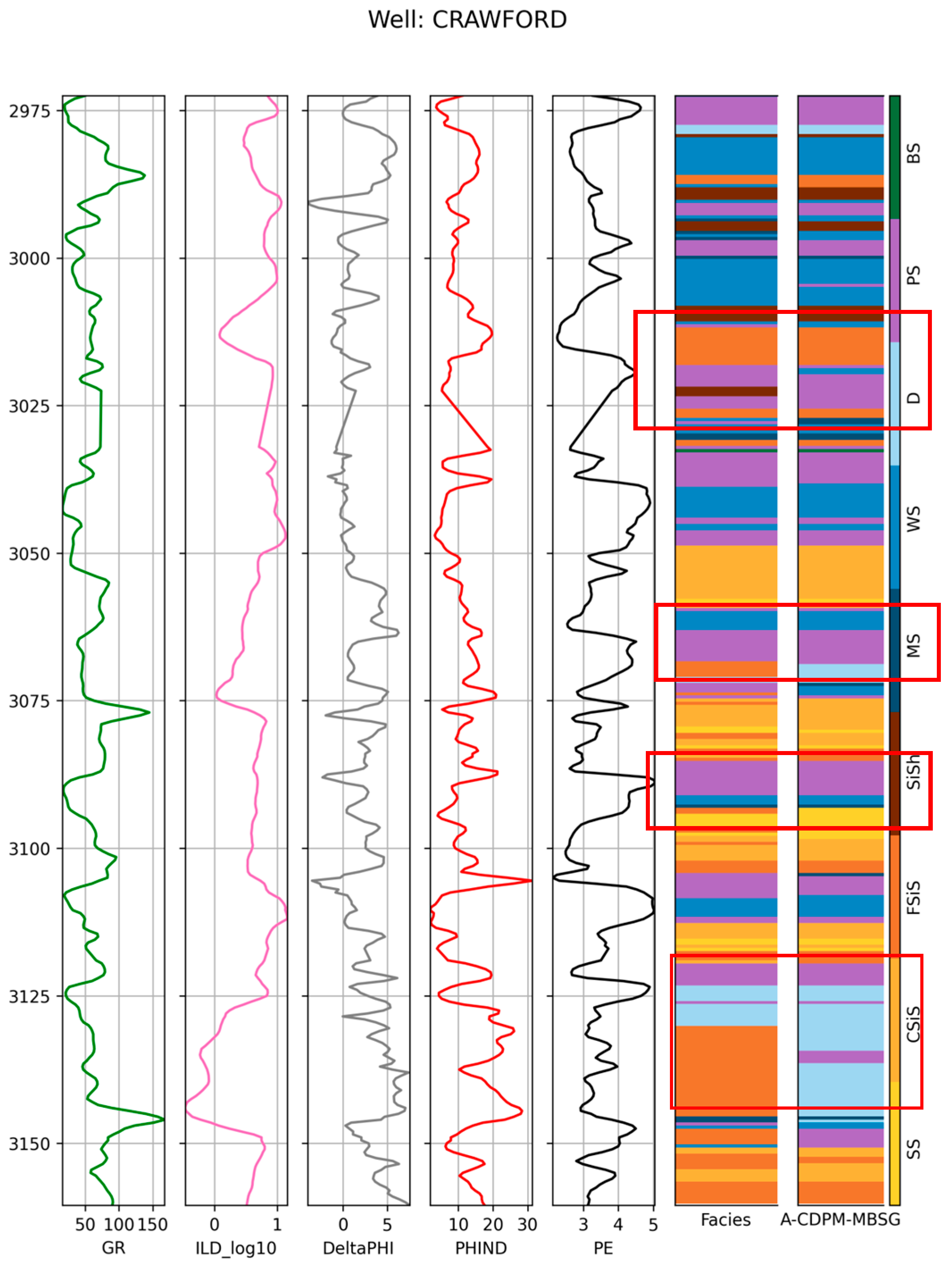
To visually illustrate the lithology recognition performance of the proposed model, Figure 15 and Figure 16 show the prediction results of the A-CDPM-MSBG model for the two blind wells, CRAWFORD and STUART, in which the misclassified intervals are explicitly annotated.

Figure 15. Visualization of Lithology Identification Results for the STUART Well.

Figure 16. Visualization of Lithology Identification Results for the CRAWFORD Well.

3.7. Computing Environment

The training and evaluation phases of the entire model were executed in a Python 3.9 environment, utilizing the PyTorch 1.12.0 deep learning framework on a Windows 11 operating system, with computations accelerated by a GeForce RTX 1050 Ti GPU.

4. Discussion

4.1. Effectiveness of A-CDPM for Data Augmentation

As shown in Figure 12, the proposed A-CDPM achieved better classification performance than the other data augmentation methods. Compared with conventional unconditional DDPM, the auxiliary classifier introduces lithology label information into the sampling process, enabling the generated well-log samples to better match specific lithology classes and the real data distribution. This class-guided generation is particularly beneficial for minority lithologies and transitional intervals, where unconditional generation is more likely to produce ambiguous samples.

The visualization results in Figure 10 and Figure 11 further support this finding. The substantial overlap between the generated and original samples in both PCA and t-SNE spaces suggests that A-CDPM preserves the dominant global structure and the main local neighborhood relationships of the original data. Such consistency helps the augmented samples improve classification performance without causing severe distributional distortion.

Compared with previous lithology-identification studies based on conventional resampling methods and GAN-based augmentation frameworks, the present results suggest that diffusion-based, class-guided generation provides a more stable and effective way to improve minority-class representation while preserving the dominant structure of the original well-log distribution. This finding extends previous generative lithology-identification studies by showing that conditional diffusion augmentation can serve not only as a data balancing tool but also as a mechanism for improving geological consistency in complex and imbalanced well-log classification tasks.

However, some limitations remain. The generated samples still show insufficient coverage in sparse and boundary regions and appear slightly more concentrated than the original data, indicating limited diversity in complex transition areas. Moreover, the first two principal components explain only 35.97% and 20.44% of the total variance, respectively, with a cumulative explained variance of 56.41%. This suggests that the two-dimensional PCA projection cannot fully reflect the similarity between the generated and original samples in the complete high-dimensional feature space. Therefore, although A-CDPM effectively preserves the dominant distribution patterns of the original data, further improvement is still needed to enhance sample diversity and better characterize complex lithological transitions.

4.2. Effect of Channel Attention on Lithology Discrimination

Figure 13 shows that the channel attention weights are unevenly distributed across latent channels for different lithologies, indicating that the model does not treat all extracted features equally but instead adaptively emphasizes more informative responses. Some channels remain highly activated across multiple lithologies, suggesting that they capture shared discriminative patterns, whereas others show clear lithology-dependent variations, reflecting enhanced class-specific representations.

This adaptive channel reweighting is particularly important for complex lithology classification. In well-log data, subtle inter-class differences are often obscured by overlapping responses, noise, and local fluctuations. Under such conditions, channel attention helps preserve weak but discriminative signals and suppress less relevant feature responses, thereby improving the recognition of rare lithologies and easily confused classes. This interpretation is consistent with the ablation results, where the introduction of channel attention increased the Accuracy, Precision, Recall, and F1-score from 76.68%, 75.67%, 74.38%, and 74.99% to 86.66%, 85.44%, 84.78%, and 85.11%, respectively. The large performance gain indicates that insufficient channel-wise feature utilization was a major limitation of the baseline model.

It should be noted that the channels in Figure 13 correspond to latent feature maps rather than the original logging variables, and therefore, they should not be directly interpreted as specific logs. Instead, these channels may encode integrated hidden responses associated with shale content, mineral composition, pore structure, and electrical properties. From this perspective, channel attention improves lithology discrimination by strengthening the discriminative capacity of combined hidden representations under complex geological conditions.

Compared with previous lithology-identification models that mainly rely on direct feature extraction without explicit channel recalibration, the present results indicate that channel attention contributes not only to global accuracy improvement but also to the enhanced recognition of rare and easily confused lithologies. This suggests that, in complex well-log classification tasks, improving channel-wise feature utilization is an important complement to data augmentation, and that the combination of generation enhancement and discriminative feature refinement is a key reason for the superior performance of the proposed framework.

4.3. Generalization Performance in Blind Well

Although the proposed model achieved the best performance in blind-well testing, its Accuracy, Precision, Recall, and F1-score were still lower than those in the main experiment, decreasing from 86.66%, 85.44%, 84.78%, and 85.11% to 75.66%, 78.56%, 73.29%, and 77.78%, respectively. Among these metrics, Recall showed the largest decline, indicating that the model was more likely to miss some lithology samples in the unseen wells, especially minority lithologies, thin interbeds, and boundary intervals.

This performance reduction may be related to inter-well heterogeneity. Differences in depositional background, diagenetic conditions, lithological assemblages, and logging-response characteristics between the training wells and the blind wells may introduce distribution discrepancies, which can weaken the transferability of the learned discriminative patterns. Consequently, the decision boundaries learned from the training wells may not generalize sufficiently to unseen wells, particularly in intervals with limited sample support or complex lithological transitions.

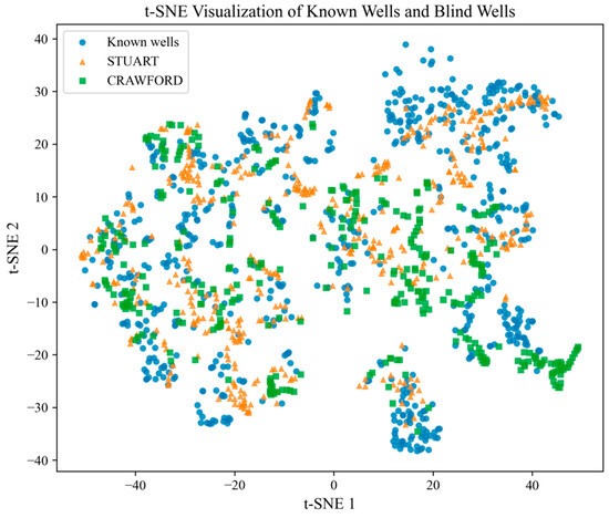
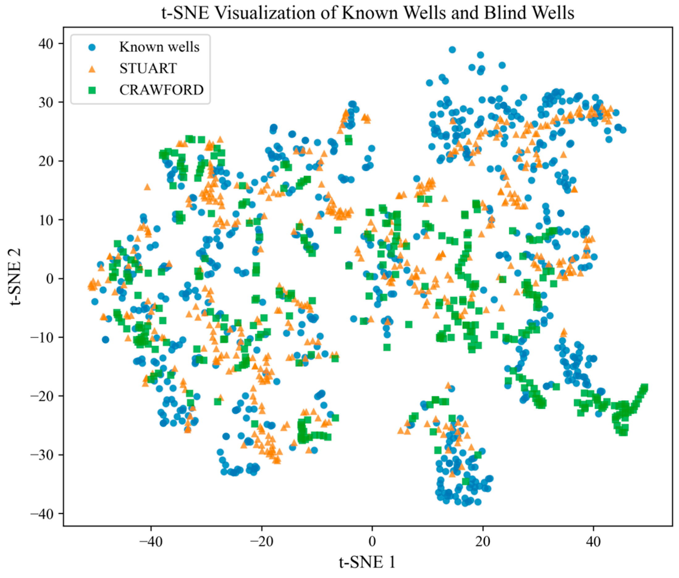
To further examine this explanation, a t-SNE visualization was added to compare the feature-space distributions of the known wells and the blind wells. As shown in Figure 17, the samples from STUART and CRAWFORD partially overlap with those from the known wells, suggesting that they share some common logging-response patterns. However, clear local distribution shifts can also be observed. In particular, CRAWFORD forms several relatively separated clusters in the projected feature space, indicating that its logging-response distribution differs from that of the known wells. This feature-space discrepancy provides visual evidence that inter-well heterogeneity may partly explain the reduced Recall in blind-well testing.

Figure 17. t-SNE Projection of Feature Distributions for Known and Blind Wells.

Nevertheless, the model still maintained relatively stable overall performance in blind-well testing, indicating that the proposed framework has promising generalization capability. These results suggest that the combination of data augmentation and feature optimization is effective in improving robustness. Future work will further investigate cross-well feature-space discrepancies using quantitative distribution-shift measurements and develop methods to enhance adaptability to potential cross-well distribution shifts, especially for boundary and minority lithologies.

5. Conclusions

This study demonstrates that the integration of auxiliary classification-guided diffusion-based data augmentation, multi-scale feature extraction, and channel-wise feature optimization can effectively improve lithology recognition under imbalanced well-log data conditions. The main findings of this study can be summarized as follows:

Compared with several representative augmentation methods, including the interpolation-based SMOTE method, the GAN-based CE-SGAN method, and the diffusion-based DDPM method, A-CDPM consistently achieved higher classification accuracy under different sampling proportions. This indicates that auxiliary classification-guided diffusion generation can better improve minority-class representation and provide more stable data supplementation for imbalanced well-log datasets.

When combined with the proposed multi-scale convolutional recognition model with channel attention and BiGRU, the final framework achieved an Accuracy of 86.66%, a precision of 85.44%, a recall of 84.78%, and an F1-score of 85.11%. The ablation results further show that the introduction of the channel attention mechanism increased Accuracy from 76.68% to 86.66%, corresponding to an improvement of 9.98 percentage points. These results confirm that the proposed framework improves lithology recognition from both the data level and the feature level: A-CDPM alleviates class imbalance through class-guided diffusion augmentation, while the channel-attention-based multi-scale model enhances key feature extraction and lithology discrimination.

Overall, the proposed framework provides an effective solution for lithology recognition in complex and imbalanced well-log datasets. Future work will focus on improving the diversity and geological consistency of generated samples, enhancing cross-well generalization ability under blind-well conditions, and extending the proposed framework to other geophysical interpretation tasks.

References

- Ismail, A.; Raza, A.; Gholami, R.; Rezaee, R. Reservoir characterization for sweet spot detection using color transformation overlay scheme. J. Pet. Explor. Prod. Technol. 2020, 10, 2313–2334. [Google Scholar] [CrossRef] [Scilit]
- Jin, H.; Yutong, C.; Xuan, L. Research status and prospects of intelligent logging lithology identification. Meas. Sci. Technol. 2025, 36, 012010. [Google Scholar] [CrossRef] [Scilit]
- Radhi, F.A.; Al-Fatlawi, O.; Kadkhodaie, A. Lithology and minerals identification from well logs for Mishrif Formation in Ratawi oilfield. Iraqi J. Chem. Pet. Eng. 2025, 26, 129–138. [Google Scholar] [CrossRef] [Scilit]
- Ashraf, U.; Zhang, H.; Thanh, H.V.; Anees, A.; Ali, M.; Duan, Z.; Mangi, H.N.; Zhang, X. A robust strategy of geophysical logging for predicting payable lithofacies to forecast sweet spots using digital intelligence paradigms in a heterogeneous gas field. Nat. Resour. Res. 2024, 33, 1741–1762. [Google Scholar] [CrossRef] [Scilit]
- Zhang, Y.-S.; Fu, J.-L.; Wu, K.-Y.; Wang, W.-R.; Jiang, Y.-H.; Zhang, S.-Q.; Li, J.; Wang, H.; Deng, L.-B.; Xu, Z.-M. Lithofacies division and intelligent identification of the lacustrine mixed rocks in the Upper Xiaganchaigou Formation in Yingxi area of the Qaidam Basin, northwestern China. J. Palaeogeogr. 2025, 14, 100270. [Google Scholar] [CrossRef] [Scilit]
- Liao, W.; Zhao, B.; Gao, C.; Wang, H.; Zhu, H. Application of domain-adaptive network with data augmentation in lithology identification of buried hill igneous rocks. Geoenergy Sci. Eng. 2025, 251, 213848. [Google Scholar] [CrossRef] [Scilit]
- Wang, J.; Li, J.; Li, K.; Li, Z.; Kang, Y.; Chang, J.; Lv, W. Borehole lithology modelling with scarce labels by deep transductive learning. Comput. Geosci. 2024, 192, 105706. [Google Scholar] [CrossRef] [Scilit]
- Zhu, X.; Zhang, H.; Ren, Q.; Zhang, L.; Ge, Y. Cost-focused intelligent reservoir logging interpretation: Evaluation of cost-sensitive active learning strategies. Eng. Appl. Artif. Intell. 2025, 158, 111630. [Google Scholar] [CrossRef] [Scilit]
- Li, H.; Sun, Y.; Qiao, S. Enhanced lithology identification with few-shot well-logging data using a confidence-enhanced semi-supervised meta-learning approach. Measurement 2025, 247, 116762. [Google Scholar] [CrossRef] [Scilit]
- Wang, A.; Zhao, S.; Xie, K.; Wen, C.; Tian, H.-l.; He, J.-B.; Zhang, W. Attention mechanism-enhanced graph convolutional neural network for unbalanced lithology identification. Sci. Rep. 2024, 14, 17319. [Google Scholar] [CrossRef] [Scilit]
- Hasnan, H.K.; Sheppard, A.; Hassan, M.H.A.; Knackstedt, M.; Abdullah, W.H. Digital core analysis: Improved connectivity and permeability characterization of thin sandstone layers in heterolithic rocks. Mar. Pet. Geol. 2020, 120, 104549. [Google Scholar] [CrossRef] [Scilit]
- Cao, M.; Gao, Z.; Yuan, Y.; Yan, Z.; Zhang, Y. A Visualization and Analysis Method by Multi-Dimensional Crossplots from Multi-Well Heterogeneous Data. Energies 2022, 15, 2575. [Google Scholar] [CrossRef] [Scilit]
- Gaafar, G.R.; Tewari, R.D.; Zain, Z.M. Overview of advancement in core analysis and its importance in reservoir characterisation for maximising recovery. In Proceedings of the SPE Asia Pacific Enhanced Oil Recovery Conference, Kuala Lumpur, Malaysia, 11–13 August 2015. D011S003R009. [Google Scholar] [CrossRef] [Scilit]
- Partovi, S.M.A.; Sadeghnejad, S. Geological boundary detection from well-logs: An efficient approach based on pattern recognition. J. Pet. Sci. Eng. 2019, 176, 444–455. [Google Scholar] [CrossRef] [Scilit]
- Liu, M.; Hu, S.; Zhang, J.; Zou, Y. Methods for identifying complex lithologies from log data based on machine learning. Unconv. Resour. 2023, 3, 20–29. [Google Scholar] [CrossRef] [Scilit]
- Ren, X.; Hou, J.; Song, S.; Liu, Y.; Chen, D.; Wang, X.; Dou, L. Lithology identification using well logs: A method by integrating artificial neural networks and sedimentary patterns. J. Pet. Sci. Eng. 2019, 182, 106336. [Google Scholar] [CrossRef] [Scilit]
- Schaller, S.; Becerra, P.; Beraus, S.; Buechi, M.W.; Mair, D.; Abadi, M.S.; Schuster, B.; Anselmetti, F.S. Data-driven lithofacies prediction of unconsolidated sediments from wireline logs. Sedimentologika 2025, 3, e31. [Google Scholar] [CrossRef] [Scilit]
- Al-Anazi, A.; Gates, I.D. On the Capability of Support Vector Machines to Classify Lithology from Well Logs. Nat. Resour. Res. 2010, 19, 125–139. [Google Scholar] [CrossRef] [Scilit]
- Shi, Y.; Liao, J.; Gan, L.; Tang, R. Lithofacies Prediction from Well Log Data Based on Deep Learning: A Case Study from Southern Sichuan, China. Appl. Sci. 2024, 14, 8195. [Google Scholar] [CrossRef] [Scilit]
- Liu, J.; Tian, F.; Zhao, A.; Zheng, W.; Cao, W. Logging Lithology Discrimination with Enhanced Sampling Methods for Imbalance Sample Conditions. Appl. Sci. 2024, 14, 6534. [Google Scholar] [CrossRef] [Scilit]
- Zhu, X.; Zhang, H.; Ren, Q.; Zhang, D.; Zeng, F.; Zhu, X.; Zhang, L. An automatic identification method of imbalanced lithology based on Deep Forest and K-means SMOTE. Geoenergy Sci. Eng. 2023, 224, 211595. [Google Scholar] [CrossRef] [Scilit]
- Mesroua, C.; Lahouel, I.; Hamrouni, B.; Bouanane, K.; Zidouni, F.; Kafi, W. Enhancing Lithology Prediction through Preprocessing Techniques and Machine Learning Models. CyberSystem J. 2025, 2, 65–70. [Google Scholar] [CrossRef] [Scilit]
- Zhao, F.; Yang, Y.; Kang, J.; Li, X. CE-SGAN: Classification enhancement semi-supervised generative adversarial network for lithology identification. Geoenergy Sci. Eng. 2023, 223, 211562. [Google Scholar] [CrossRef] [Scilit]
- Zhang, P.; Ren, J.; Zhao, F.; Li, X.; He, H.; Jia, Y.; Shao, X. MS-CGAN: Fusion of conditional generative adversarial networks and multi-scale spatio-temporal features for lithology identification. J. Appl. Geophys. 2024, 230, 105531. [Google Scholar] [CrossRef] [Scilit]
- Qian, H.; Geng, Y.; Wang, H. Lithology identification based on ramified structure model using generative adversarial network for imbalanced data. Geoenergy Sci. Eng. 2024, 240, 213036. [Google Scholar] [CrossRef] [Scilit]
- Zhao, F.; Lv, H.; Zhao, Z.; Li, X.; Liu, M. Lithology identification method combining attribute generation group and generative adversarial network. Earth Sci. Inform. 2025, 18, 375. [Google Scholar] [CrossRef] [Scilit]
- Ho, J.; Jain, A.; Abbeel, P. Denoising diffusion probabilistic models. Adv. Neural Inf. Process. Syst. 2020, 33, 6840–6851. [Google Scholar]
- Lee, D.; Ovanger, O.; Eidsvik, J.; Aune, E.; Skauvold, J.; Hauge, R. Latent diffusion model for conditional reservoir facies generation. Comput. Geosci. 2025, 194, 105750. [Google Scholar] [CrossRef] [Scilit]
- Xu, M.; Song, S.; Mukerji, T. DiffSim: Denoising diffusion probabilistic models for generative facies geomodeling. Int. Meet. Appl. Geosci. Energy Expand. Abstr. 2024, 43, 1660–1664. [Google Scholar] [CrossRef] [Scilit]
- Ovanger, O.; Lee, D.; Eidsvik, J.; Hauge, R.; Skauvold, J.; Aune, E. A statistical study of latent diffusion models for geological facies modeling. Math. Geosci. 2025, 57, 1135–1159. [Google Scholar] [CrossRef] [Scilit]
- Meng, H.; Lin, B.; Zhang, R.; Jin, Y. A missing well-logs imputation method based on conditional denoising diffusion probabilistic models. SPE J. 2024, 29, 2165–2180. [Google Scholar] [CrossRef] [Scilit]
- Zhao, F.; Zhao, Z.; Lv, H.; Zhang, P.; Li, X. Lithology identification of imbalanced well log data based on diffusion model and multiscale CNN. Math. Geosci. 2025, 57, 1283–1304. [Google Scholar] [CrossRef] [Scilit]
- Sun, W.; Zhao, J.; Peng, S.; Huang, W.; Li, H. Physically consistent joint prediction of porosity and shale volume via core-calibrated deep learning in well-consolidated sandstones. Sci. Rep. 2025, 15, 31326. [Google Scholar] [CrossRef] [Scilit]
- Dubois, M.K.; Bohling, G.C.; Chakrabarti, S. Comparison of four approaches to a rock facies classification problem. Comput. Geosci. 2007, 33, 599–617. [Google Scholar] [CrossRef] [Scilit]
- Ronneberger, O.; Fischer, P.; Brox, T. U-Net: Convolutional Networks for Biomedical Image Segmentation. In Proceedings of the International Conference on Medical Image Computing and Computer-Assisted Intervention, Munich, Germany, 5–9 October 2015; pp. 234–241. [Google Scholar] [CrossRef] [Scilit]
- Lecun, Y.; Bottou, L.; Bengio, Y.; Haffner, P. Gradient-based learning applied to document recognition. Proc. IEEE 1998, 86, 2278–2324. [Google Scholar] [CrossRef] [Scilit]
- Liu, Y.; Huang, L.; Li, J.; Zhang, W.; Sheng, Y.; Wei, Z. Multi-task learning based on geometric invariance discriminative features. Appl. Intell. 2023, 53, 3505–3518. [Google Scholar] [CrossRef] [Scilit]
- Hu, J.; Shen, L.; Sun, G. Squeeze-and-excitation networks. In Proceedings of the IEEE Conference on Computer Vision and Pattern Recognition, Salt Lake City, UT, USA, 18–23 June 2018; pp. 7132–7141. [Google Scholar] [CrossRef] [Scilit]
- Imamverdiyev, Y.; Sukhostat, L. Lithological facies classification using deep convolutional neural network. J. Pet. Sci. Eng. 2019, 174, 216–228. [Google Scholar] [CrossRef] [Scilit]
Disclaimer/Publisher’s Note: The statements, opinions and data contained in all publications are solely those of the individual author(s) and contributor(s) and not of MDPI and/or the editor(s). MDPI and/or the editor(s) disclaim responsibility for any injury to people or property resulting from any ideas, methods, instructions or products referred to in the content. |
© 2026 by the authors. Licensee MDPI, Basel, Switzerland. This article is an open access article distributed under the terms and conditions of the Creative Commons Attribution (CC BY) license.