Abstract
Stable attitude control of unmanned or autonomous operations of vehicles moving in three spatial dimensions is essential for safe and reliable operations. Rigid body attitude control is inherently a nonlinear control problem, as the Lie group of rigid body rotations is a compact manifold and not a linear (vector) space. Prior research has shown that the largest possible domain of convergence is provided by smooth attitude feedback control laws are obtained using a Morse function on as a measure of the attitude stabilization or tracking error. A polar Morse function on has four critical points, which precludes the possibility of global convergence of the attitude state. When used as part of a Lyapunov function on the state space (the tangent bundle ) of attitude and angular velocity, it gives a globally continuous state-dependent feedback control scheme with the minimum of the Morse function as the almost globally asymptotically stable (AGAS) attitude state. In this work, we explore the use of explicitly time-varying gains for Morse functions for rigid body attitude control. This strategy leads to discrete switching of the indices of the three non-minimum critical points that correspond to the unstable equilibria of the feedback system. The resulting time-varying feedback controller is proved to be AGAS, with the additional desirable property that the time-varying gains destabilize the (locally) stable manifolds of these unstable equilibria. Numerical simulations of the feedback system with appropriate time-varying gains show that a trajectory starting from an initial state close to the stable manifold of an unstable equilibrium, converges to the desired stable equilibrium faster than the corresponding feedback system with constant gains.
1. Introduction
Vehicles moving in three spatial dimensions, which include aerial, space and underwater vehicles, require attitude control. The vehicles can be modeled as a rigid body with actuators that are used for attitude and translational motion. In this work, we consider control of the attitude motion for maneuverable vehicles without any constraints on the motion. Rigid body attitude is uniquely and globally represented on the Lie group , which is a compact manifold and not a vector (linear) space. This makes control of rigid body rotational motion on the state space , the tangent bundle of consisting of all attitudes (orientations) and angular velocities, an inherently nonlinear control problem. Prior research on attitude stabilization and control has shown that global stabilization on with continuous state feedback is not possible [1,2,3].
Instead, the best possible outcome with continuous state feedback is almost global asymptotic stability of desired trajectories or states on [2,3,4]. This best possible outcome is achieved by use of Morse or Morse-Bott functions on , as part of Lyapunov functions on the state space . Consequently, Morse and Morse–Bott functions are necessary to design Lyapunov functions for rigid body control and estimation with guarantees of almost global domains of convergence. Polar Morse functions on have a critical set with cardinality four, while Morse-Bott functions on have a connected set of critical points; the sets of critical points for both these types of functions are of zero (Lebesgue) measure on . Their use as part of Lyapunov functions produce feedback systems whose equilibria on correspond to the critical points (attitudes) of the Morse (or Morse–Bott) function on . The existence of multiple equilibria precludes global asymptotic stability of a single equilibrium state of the continuous state feedback system. By formulating the function appropriately, one can obtain almost global asymptotic stability (AGAS) for the desired attitude state as an equilibrium, while the other equilibria are confined to a set of measure zero in .
Designs using constant gain Morse functions have a limitation in applications that involve large rotations but need fast convergence to a desired attitude. The control approach given in this work is also robust to external disturbance torques due to its rapid convergence and large domain of attraction. In this sense, it is complementary to our previous work on attitude control on using integral feedback [5]. Another use case for the control scheme given here is for attitude synchronization of multi-agent rigid body systems (MARBS), where certain network topologies admit stable but undesirable non-consensus equilibria that correspond to critical points of the Morse or Morse-Bott function that prevent convergence to the consensus configuration for the MARBS network [6,7]. Constant gains fix the Hessian of the Morse function at each critical point, and therefore limit our ability to alter stability properties of the critical point without changing the function’s continuity and resorting to hybrid switching strategies. A backstepping-based approach for rigid body control using Morse-Lyapunov functions appeared in [8]. Recent work on feedback reshaping [6,9,10], decentralized consensus protocol [11] for relative attitude control, and hybrid strategies for trajectory tracking control [12] have demonstrated the need for more flexible approaches to avoid or destabilize undesired equilibria.
In this work, we design and analyze a new class of polar Morse functions that have continuously time-varying positive gains, for stable and robust attitude control. The principal motivations are two-fold. The time-dependence of gains in the Morse function modifies the local properties (the gradient and Hessian) of the non-minimum critical points, and this changes the properties of the dynamics near the equilibria corresponding to these critical points, without altering the global stability properties or using discontinuous or hybrid control. The second motivation of practical interest is the use of these functions for attitude synchronization in multi-agent systems. We hypothesize that using time-varying Morse functions for relative attitude measure in a network of rigid bodies can destabilize or remove undesirable non-consensus and partial consensus [7] equilibria arising from certain graph topologies, and thus recover almost global synchronization without hybrid switching or discontinuous control. Preliminary related ideas have appeared in feedback-reshaping and time-varying formation control literature [13,14,15], but a systematic analysis of Morse functions with continuous time-varying gains for single rigid body control is, to the best of our knowledge, unexplored. This work, which concentrates on developing important fundamental results for single rigid-body attitude control with a continuous time-varying state feedback, can serve as a foundation for future work on attitude synchronization and control of MARBS.
The remainder of this article is organized as follows. Section 2 defines the problem statement followed by Section 3 containing analysis and some basic results from prior research using (constant gain) Morse functions. It also introduces time-varying Morse functions, establishes some important results, and contrasts it with results obtained using constant Morse functions. This section lays the groundwork for the attitude control approach presented in this article. Next, Section 4 formulates a time-varying controller using a Morse function with time-varying gains for attitude control. This is followed by Section 5, which provides numerical simulation results for the designed controller, highlighting the advantages of the proposed time-varying Morse function. Lastly, Section 6 concludes this article by summarizing contributions and giving planned future directions.
2. Problem Statement
Consider a rigid body with a body-fixed coordinate frame centered at the center of mass. Let R be the rotation matrix from frame to an inertial coordinate frame . The attitude kinematics and dynamics are described by:
where is the angular velocity of the rigid body in frame , is the inertia-like matrix of the rigid body, and is the control torque acting on that rigid body in frame . If denotes a trajectory on , the tangent vector at is given by:
where and is the Lie algebra of , represented by skew-symmetric matrices. This Lie algebra corresponds to the three-dimensional Euclidean vector space , with the angular velocity vector being mapped by the map. This map is a vector space isomorphism from 3D vectors in to skew-symmetric matrices in , and the cross superscript is used as this is equivalent to the cross product operator matrix, i.e., for vectors . The attitude dynamics (2) generates trajectories in the state space . Consider attitude control of the rigid body with a control law designed for to stabilize the attitude trajectory to .
3. Morse Function on SO(3) with Time-Varying Gains
Let denote the trace inner product defined by:
where denotes the trace of a matrix. Consider a polar Morse function defined on the Lie group as:
where is a rotation matrix, and is a constant positive diagonal matrix with . A variation of R on is given by:
where and is the skew-symmetric cross-product operator matrix associated with .
3.1. First Variation of the Morse Function
The first variation of is given by:
Using the commutative property of trace operator and orthogonality of symmetric and skew-symmetric matrices under the trace inner product, Equation (6) simplifies to:
and is the inverse of the cross-product operator map . The following result is used in our main result in the next section, and its detailed proof is given in [16]. For brevity, we omit the proof in this paper.
Lemma 1.
Now consider , a time-varying positive diagonal matrix. Then the Morse function becomes:
Next we evaluate the first variation of U, due to variations in R. That is, we compute:
where is a curve on with and , for some . Thus, the first variation of U with respect to R is:
As the Morse function in (10) varies explicitly with time, its gradient on also varies explicitly with time.
3.2. Analysis of Equilibria on
Using the identity: , Equation (12) simplifies to
where and is as defined by Equation (7). It can be readily verified by inspection that
where , are the column vectors of the identity matrix.
The necessary condition for critical points of the Morse function in Equation (10) is , which implies that , or equivalently , at the critical points. Therefore, the set of critical points is
Moreover, from Equation (15), implies that . Therefore, set in Equation (16) is given by its elements as:
, , and denote ( rad) rotations about the body frame’s first, second and third coordinate axes, respectively. Note that this set of critical points with time-varying is identical to that obtained with constant K, which can be readily obtained by setting the right side of Equation (7) to zero. The second variation of Equation (10) is obtained by applying the variation operator to Equation (12), as:
where denotes the differential of . Using the trace orthogonality property of symmetric and skew-symmetric matrices, Equation (18) further simplifies to
The following result gives the Hessian matrices for each element in the set of critical points of .
Proposition 1.
The Hessian matrices for the critical points of the Morse-function with time-varying gains , are given by:
Proof.
Evaluating the second variation of the Morse function given by Equation (10) on the set at an instant of time t, gives:
Evaluating Equation (21) at each of the four critical points, we get:
We evaluate the Hessian matrix evaluated for by taking second partial derivatives of with respect to . This is obtained as:
where . For , we get:
because the critical values are diagonal matrices. In addition, , which leads to the following expression for the Hessian matrices evaluated at these critical points:
Substituting for , based on Equation (23) evaluated at each of the critical points into Equation (24), leads to the Hessian matrices given explicitly by Equation (20) at these critical points. □
Equation (20) reveals that the Hessian of the Morse function evaluated at critical points in the set (16) depends on time because of ; this is unlike the case with constant K. This directly affects the indices of these critical values on , which in turn influences the stability properties of the equilibria on that these critical points correspond to in the feedback system. This is due to the fact that the eigenvalues of for are time-varying and may be positive, negative or even momentarily zero depending on the relative values of the . The only critical point that has a positive definite Hessian and therefore a zero index for all time is the identity , which corresponds to the desired equilibrium state . In summary, the time-varying positive diagonal gain matrix ensures that the non-minimum critical points of the Morse function that are in the set , have time-varying indices.
Remark 1.
The index of a critical point (of the Morse function) is the number of negative eigenvalues of its Hessian, , for . If is constant, then the indices of and are 0, 1, 2 and 3, respectively with the minimum attained at , given that . However, when is time-varying, the number of positive and negative eigenvalues of the Hessian at any of the three non-minimum critical points of the Morse function (i.e., any point in the set ), may switch with time depending on . As the index values can vary with time for , the dimensions of stable and unstable manifolds associated with these critical points also switch with time. As can be seen from Equation (20), a switch in the index of one of these three critical points occurs when for , . This results in discrete switching of the index values at these critical points depending on the instantaneous inequality constraint between the elements of the positive diagonal matrix . The indices of the critical points give the dimensions of the stable manifolds of the equilibria of the feedback system corresponding to these critical points. The dimension of the stable manifold is calculated as , where 6 is the total dimension of the state-space . Therefore, the stable manifolds and their dimensions vary over time for the equilibrium points corresponding to the critical points of .
4. AGAS Attitude Control Law
The following statement gives a feedback control law on the state space to asymptotically stabilize the desired attitude and angular velocity state . It uses a particular design of the time-varying gains to obtain this result.
Theorem 1.
Consider a positive diagonal time-varying such that where are diagonal and , , and is continuous, non-negative, and time-periodic with period T. Consider the attitude control law for the rigid body given by:
where , . This control law makes the state almost globally asymptotically stable (AGAS) and locally exponentially stable.
Proof.
The proof is given in two steps. The first step considers the velocity kinematics, where we define a desired angular velocity profile that is guaranteed to steer the attitude towards the identity attitude I. In the second step, the attitude dynamics is considered, where we formulate the control torque law that forces the true angular velocity of the rigid body to follow the desired angular velocity with finite-time stable (FTS) convergence.
Consider the polar Morse function on given by
which depends on the constant part of as defined in the statement. The time derivative of (26) is given by
where and is the inverse of the cross-product operator map defined by Equation (2). A kinematic control law that leads to almost global asymptotically stable (AGAS) convergence of R to described by (1) is given by
where according to the properties of . Setting the true angular velocity equal to the desired angular velocity , and substituting (28) into the expression (27) for the time derivative of , gives:
Simplifying (29) using (28) and the observation that the vectors , are mutually orthogonal, leads to:
Given that both is positive and is non-negative diagonal (i.e., , ), Equation (30) leads to the conclusion that:
In inequality (31), the time derivative of the constant gain Morse function when . The only (global) minimum of is at , while and are saddle points with indices 1 and 2 respectively. The global maximum of over is attained at . Therefore, with the kinematic control law (28), all trajectories on that do not start on the stable manifolds of and , or at , converge to . This leads to being the AGAS equilibrium for this kinematic (velocity level) control system on . In addition, applying Lemma 1 to inequality (31), we see that in the neighborhood of given by Equation (9). This leads to local exponential stability of the kinematic control law (28) at .
The next step of this control scheme is to track the desired angular velocity profile given by the kinematic-level control law (28) so that the true angular velocity converges to this desired profile in a finite time interval. For this, we define the angular velocity tracking error as . Consider the attitude dynamics of the body given by the second of Equation (1), where is the inertia matrix. Define the following energy-like Lyapunov function of the angular velocity tracking error:
The time derivative of this Lyapunov function along the trajectories of (1) is given by:
Substituting the finite-time stable control law (25) into expression (33) for and using the relation results in,
Therefore, from (34) and [17], we conclude that in finite time, with the settling time upper-bounded as follows:
where is the initial value of the Lyapunov function in (32) and is the initial tracking error in angular velocity. In summary, the control law (25) ensures FTS convergence of to , which in turn ensures AGAS convergence of to according to the kinematic control law (28). □
For numerical simulation studies, this work considers a particular structure of given by:
where , , is the oscillation frequency and is an initial phase, for . In Equation (36), as the diagonal elements are periodically modulated positive functions, the conditions ; ; are satisfied at most at isolated instants in time for almost all choices of . Therefore, the relative ordering among the diagonal elements of changes repeatedly as time evolves. These changes lead to discrete switching of the indices of the three non-minimum critical points as explained in Remark 1 of Section 3. As a result, the stable manifolds of the unstable equilibria corresponding to these critical points , or have changing dimensions and changing structures, and the feedback system cannot settle into these stable manifolds for all time.
5. Numerical Simulation Results
In this section, a comparative set of numerical simulations with constant gain K and time-varying gain of the Morse function is presented. The continuous time dynamics is discretized for numerical simulations in computer. The resulting discrete time dynamics is in the form of a Lie group variational integrator (LGVI) [18], obtained by applying the discrete Lagrange–d’Alembert principle [19,20,21]. Consider an interval of time separated into N equal-length subintervals for , with and is the time step size. The discrete-time equations are:
For the time-varying gains of the Morse function, we choose the as described in (36), with:
For the constant gain Morse function, the gains are selected as . The simulated time period is 150 s. The gain matrix for the dynamic level controller (25) is with . The inertia tensor of the rigid body is kg·m2. Figure 1, Figure 2 and Figure 3 show comparative simulation results for constant K versus time-varying with initial attitudes of the rigid body given by , and , respectively. The initial angular velocity is chosen as for all three cases. Figure 1a, Figure 2a and Figure 3a show the principal rotation angle profiles for time-varying converging to zero (corresponding to identity attitude ), whereas with the constant K it remains trapped at the initial attitude , , , respectively. This behavior arises because the time-varying induces discrete switching of the critical points of the Morse function, thereby preventing the system response from being trapped at the initial attitude, unlike in the constant K case. Figure 1b, Figure 2b and Figure 3b show the norm of angular velocity profiles, and Figure 1c, Figure 2c and Figure 3c shows the variation of norm of control torque. The small differences in the peak magnitudes of the control torque in Figure 1c, Figure 2c and Figure 3c are due to the selections of the diagonal entries of the time-varying and the inertia matrix . These numerical simulation demonstrate the usefulness of time-varying gains for the Morse function as an attitude measure, and the role of the resulting time-varying state feedback controller in destabilizing the local stable manifolds of unstable equilibria.
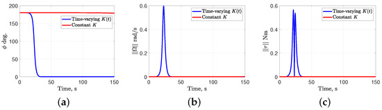
Figure 1.
Comparative simulation results with time-varying and constant gain Morse functions with . (a) Principal rotation angle; (b) Norm of angular velocity; (c) Norm of control torque.
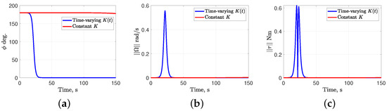
Figure 2.
Comparative simulation results with time-varying and constant gain Morse functions with . (a) Principal rotation angle; (b) Norm of angular velocity; (c) Norm of control torque.
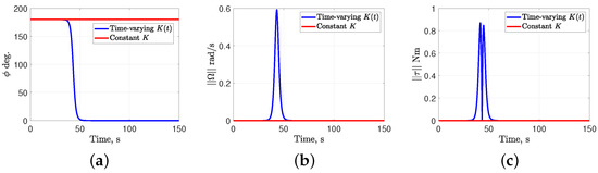
Figure 3.
Comparative simulation results with time-varying and constant gain Morse functions with . (a) Principal rotation angle; (b) Norm of angular velocity; (c) Norm of control torque.
6. Conclusions
This work provides a continuous time-varying state dependent feedback attitude controller on based on Morse functions with time-varying gains. As a result, the stable manifolds of the undesirable equilibria for the feedback system of the rigid body are disrupted because the indices of the non-minimum critical points corresponding to these equilibrium points switch discretely in time. The only always stable equilibrium on is the identity attitude with zero angular velocity. Simulation results confirm that the time-varying Morse function can prevent the system response from “getting stuck" near the undesired equilibria of the feedback system and can achieve convergence to the identity attitude. Future work will extend these results to coordinated relative-attitude control for networks of unmanned aerial vehicles modeled as multi-agent rigid-body systems (MARBS). A key direction is the design of distributed, time-varying gain matrices that shape agent-wise Morse functions and prevent the formation of undesired equilibria in the MARBS network. Another planned future research topic in this direction, is to analyze MARBS with complex but more practical graph topologies of the communications network, such as for MARBS with nearest neighbor communication.
Author Contributions
Conceptualization, A.K.S.; methodology, A.K.S. and N.S.; software, N.S.; validation, N.S. and A.K.S.; formal analysis, A.K.S.; investigation, N.S.; resources, A.K.S.; data curation, N.S.; writing—original draft preparation, N.S.; writing—review and editing, A.K.S.; visualization, N.S.; supervision, A.K.S.; project administration, A.K.S.; funding acquisition, A.K.S. All authors have read and agreed to the published version of the manuscript.
Funding
This research was funded by US National Science Foundation (NSF) grant numbers 2132799 and 2343062.
Data Availability Statement
Data, including computer codes used for simulations reported in this paper, will be made available through the US NSF Public Access Repository (NSF PAR) as part of project reports for the projects under which this research was supported. This data will be publicly accessible.
Acknowledgments
The authors acknowledge insights provided by helpful discussions with Eric Butcher at the University of Arizona.
Conflicts of Interest
The authors declare no conflict of interest.
References
- Bhat, S.; Bernstein, D. A Topological Obstruction to Continuous Global Stabilization of Rotational Motion and the Unwinding Phenomenon. Syst. Control Lett. 2000, 39, 63–70. [Google Scholar] [CrossRef]
- Chaturvedi, N.; McClamroch, N. Almost global attitude stabilization of an orbiting satellite including gravity gradient and control saturation effects. In Proceedings of the American Control Conference, Minneapolis, MN, USA, 14–16 June 2006. [Google Scholar] [CrossRef]
- Chaturvedi, N.; Sanyal, A.; McClamroch, N. Rigid-body attitude control. Control Syst. IEEE 2011, 31, 30–51. [Google Scholar] [CrossRef]
- Koditschek, D.E. The application of total energy as a Lyapunov function for mechanical control systems. Contemp. Math. 1989, 97, 131. [Google Scholar] [CrossRef]
- Eslamiat, H.; Wang, N.; Hamrah, R.; Sanyal, A.K. Geometric Integral Attitude Control on SO(3). Electronics 2022, 11, 2821. [Google Scholar] [CrossRef]
- Butcher, E.A.; Maadani, M. Rigid Body Attitude Cluster Consensus Control on Weighted Cooperative-Competitive Networks. In Proceedings of the 2024 American Control Conference (ACC), Toronto, ON, Canada, 10–12 July 2024; pp. 3049–3054. [Google Scholar] [CrossRef]
- Srinivasu, N.; Hashkavaei, N.S.; Sanyal, A.K.; Butcher, E.A. Coordinated Relative Attitude Control and Synchronization of a Multi-body Network of Vehicles. In Proceedings of the 2025 American Control Conference (ACC), Denver, CO, USA, 8–10 July 2025; pp. 1198–1203. [Google Scholar] [CrossRef]
- Nazari, M.; Maadani, M.; Butcher, E.A.; Yucelen, T. Morse-Lyapunov-Based Control of Rigid Body Motion on TSE(3) via Backstepping. In Proceedings of the 2018 AIAA Guidance, Navigation, and Control Conference, Kissimmee, FL, USA, 8–12 January 2018. [Google Scholar] [CrossRef]
- Maadani, M.; Butcher, E.A. Pose consensus control of multi-agent rigid body systems with homogenous and heterogeneous communication delays. Int. J. Robust Nonlinear Control 2022, 32, 3714–3736. [Google Scholar] [CrossRef]
- Mathavaraj, S.; Butcher, E.A. Rigid-body attitude control, synchronization, and bipartite consensus using feedback reshaping. J. Guid. Control Dyn. 2023, 46, 1095–1111. [Google Scholar] [CrossRef]
- Butcher, E.A.; Spaeth, V. Decentralized Consensus Protocols on SO(4)N and TSO(4)N with Reshaping. Entropy 2025, 27, 743. [Google Scholar] [CrossRef] [PubMed]
- Casau, P.; Sanfelice, R.G.; Cunha, R.; Silvestre, C. A globally asymptotically stabilizing trajectory tracking controller for fully actuated rigid bodies using landmark-based information. Int. J. Robust Nonlinear Control 2015, 25, 3617–3640. [Google Scholar] [CrossRef]
- Dong, X.; Yu, B.; Shi, Z.; Zhong, Y. Time-varying formation control for unmanned aerial vehicles: Theories and applications. IEEE Trans. Control Syst. Technol. 2014, 23, 340–348. [Google Scholar] [CrossRef]
- Dong, X.; Hu, G. Time-varying formation control for general linear multi-agent systems with switching directed topologies. Automatica 2016, 73, 47–55. [Google Scholar] [CrossRef]
- Maadani, M.; Butcher, E.A. 6-DOF consensus control of multi-agent rigid body systems using rotation matrices. Int. J. Control 2022, 95, 2667–2681. [Google Scholar] [CrossRef]
- Bohn, J.; Sanyal, A.K. Almost global finite-time stabilization of rigid body attitude dynamics using rotation matrices. Int. J. Robust Nonlinear Control 2016, 26, 2008–2022. [Google Scholar] [CrossRef]
- Bhat, S.; Bernstein, D. Finite-Time Stability of Continuous Autonomous Systems. SIAM J. Control Optim. 2000, 38, 751–766. [Google Scholar] [CrossRef]
- Nordkvist, N.; Sanyal, A.K. A Lie Group Variational Integrator for Rigid Body Motion in SE(3) with Applications to Underwater Vehicle Dynamics. In Proceedings of the 49th IEEE Conference on Decision and Control (CDC), Atlanta, GA, USA, 15–17 December 2010; pp. 5414–5419. [Google Scholar] [CrossRef]
- Marsden, J.; West, M. Discrete mechanics and variational integrators. Acta Numer. 2001, 10, 357–514. [Google Scholar] [CrossRef]
- Hairer, E.; Lubich, C.; Wanner, G. Structure-preserving algorithms for ordinary differential equations. In Geometric Numerical Integration, 2nd ed.; Springer Series in Computational Mathematics; Springer: Berlin/Heidelberg, Germany, 2006; Volume 31, pp. xviii+644. [Google Scholar] [CrossRef]
- Schmitt, J.M.; Leok, M. Properties of Hamiltonian variational integrators. IMA J. Numer. Anal. 2018, 38, 377–398. [Google Scholar] [CrossRef]


Disclaimer/Publisher’s Note: The statements, opinions and data contained in all publications are solely those of the individual author(s) and contributor(s) and not of MDPI and/or the editor(s). MDPI and/or the editor(s) disclaim responsibility for any injury to people or property resulting from any ideas, methods, instructions or products referred to in the content. |
© 2025 by the authors. Licensee MDPI, Basel, Switzerland. This article is an open access article distributed under the terms and conditions of the Creative Commons Attribution (CC BY) license (https://creativecommons.org/licenses/by/4.0/).