Bumper Impact Test Damage and Static Structural Characterization in Hybrid Composite Aided by Numerical Simulation and Machine Learning Analysis

Abstract

Modern automotive design has increasingly embraced plastics for bumper construction; however, it can lead to material degradation. To overcome these limitations, the automotive industry is turning to fiber–resin material, namely carbon–epoxy composites. Our research focuses on determining the effects of fiber orientation and angle alignment on the structural stress of the car bumper, examining the hybrid material (carbon–epoxy reinforced by CFRP) in static structural tests, and performing dynamic impact tests at various speeds, applying the Tsai–Wu criterion as a basic failure model. However, Tsai–Wu’s failure in numerical analysis highlights the limitation of not being able to experimentally distinguish between failure modes and their interaction coefficients. To address this issue, we employ ANSYS^® 2024 R1 with a Fortran program, which enables more accurate estimation of failure behavior, resulting in an average error of 13.19%. To identify research gaps, machine learning (ML) plays a vital role in predicting parameter values and assessing data normality using various algorithms. By combining ML and FEA simulations, the result shows strong data performance. Bridging from 2 mm mesh sizing of 50% carbon–epoxy woven/50% CFRP laminate in 6 mm thickness at 0° orientation shows the most distributed shear stresses and deformation, which converged toward stable values. For comprehensive research, total deformation was included in ML analysis as a second target to build a multivariate analysis. Overall, Random Forest (RF) is the best-performing model, indicating superior robustness for modeling shear stress and total deformation.

1. Introduction

Road traffic accidents remain one of the leading causes of injury and mortality worldwide [1]. With rapid urbanization and a growing global population, personal and commercial transportation have become increasingly indispensable, leading to an exponential increase in the number of vehicles on our roads. Technological advancements have enabled drivers to cover greater distances in less time. Yet, this very capability, when coupled with lapses in attention and habitual speeding, has dramatically elevated the risk of collisions. As cars cruise at ever-higher speeds, the likelihood of severe and often fatal crashes intensifies, driving road traffic fatalities to alarming levels. Based on the World Health Organization data through Chang et al.’s [2] research, fatalities from road traffic collisions have climbed markedly over the past two decades, rising from approximately 1.15 million in 2000 to around 1.35 million by 2018. These figures mean that of the roughly 56.9 million people who die each year, nearly 2.4% succumb to injuries sustained in vehicle crashes, making traffic accidents the eighth leading cause of death worldwide. Beyond the human toll, these losses carry significant economic and social costs, disproportionately affecting young adults and low and middle income countries [3,4]. The growing magnitude of this public health crisis underscores the imperative for enhanced vehicle safety technologies, more rigorous enforcement of traffic regulations, and coordinated global efforts such as the UN’s Decade of Action for Road Safety, with the target of preventing at least 50% of road traffic deaths and injuries by 2030 [5]. By focusing on vehicle safety technologies to support safety regulation, the most affected component in such incidents is the car bumper, which plays a vital role in absorbing and dissipating kinetic energy during crashes, thereby improving safety and enhancing the car’s performance [6]. As the first line of defense in frontal and rear-end collisions, the bumper is crucial not only in minimizing damage to the vehicle’s body but also in reducing the force transmitted to passengers, thereby lowering the risk of severe injury or death. However, the increasing frequency of high-impact accidents underscores the need for more resilient, efficient bumper designs.

Modern automotive design has increasingly embraced plastics for bumper construction, leveraging their unique blend of functional and aesthetic benefits. Unlike traditional metal counterparts, plastic bumpers can be engineered from recyclable polymers, aligning with environmental sustainability goals and facilitating end-of-life material recovery [7]. Their inherent flexibility allows for cost-effective repairs; minor dents and scratches can often be remedied with simple heat treatments or plastic fillers rather than full panel replacements [8], thereby reducing maintenance expenses for vehicle owners. Furthermore, advanced plastic composites now match or even exceed the energy-absorbing performance of steel, as demonstrated by Tsirogiannis et al. [9], dissipating collision forces effectively to protect both the vehicle’s structure and its occupants. Beyond these practical merits, plastics offer designers a broader palette of textures, colors, and form factors [10], enabling sleek, aerodynamic profiles that enhance a vehicle’s visual appeal without compromising safety.

Over time, repeated exposure to ultraviolet light and temperature fluctuations can lead to material degradation, causing discoloration, surface cracking, and embrittlement that compromise appearance and structural integrity [11]. Additionally, conventional thermoplastics, such as polypropylene bumpers, may lack sufficient stiffness and strength for high-energy impacts [12], sometimes transferring more force to the underlying vehicle structures and occupants. To overcome these limitations, the automotive industry is increasingly turning to fiber–resin-reinforced composites [13], such as carbon fiber laminates, which combine a polymer matrix with high fiber compatibility [14]. These hybrid materials not only retain the lightweight, form-flexible advantages of plastics but also deliver superior specific stiffness and strength, enhanced fatigue resistance, and improved crashworthiness through tailored layups that dissipate energy more efficiently. By adopting composite bumpers, manufacturers can achieve a harmonious balance of aesthetics, sustainability, and safety, providing vehicles with durable bumpers that withstand harsh environmental conditions and enhanced protection in severe collisions.

Several relevant studies demonstrate the potential of virtual testing for composite bumper crash evaluation. However, limitations in scope and discussion create this gap. Rajan et al. [15] examined primarily static structural response rather than dynamic impact (impact test), and their use of E-glass fiber as a stainless-steel alternative yielded limited performance insights for high-energy events. In contrast, our work targets carbon–epoxy composite materials with substantially higher specific stiffness/strength and introduces hybridization with CFRP as a core novelty in dynamic tests. Moreover, Yeshanew et al. [16] further relied on von Mises stress, which is generally unsuitable for identifying failure in anisotropic laminates, and did not report fiber orientations; both omissions are explicitly addressed in our methodology. Furthermore, Abrar et al. [17] share key shortcomings: they did not clearly model or visualize the wall–bumper contact interface in their contour results and omitted time-resolved (dynamic) visualizations of the impact event. In this work, we address these gaps by using a linear elastic constitutive model and anisotropic failure criterion (Tsai–Wu) to measure shear-stress response during a crash event, implementing an explicit wall–bumper contact definition with reported parameters and providing visualizations to capture the evolution of damage under dynamic loading (various speed tests with constant time). However, based on Jian et al.’s [18] explanation, the linear elastic model is a straightforward model and cannot capture the complex constitutive properties (rate-dependent behavior, progressive damage, delamination, and nonlinear failure evolution), thus limiting its application and accuracy. Although limited, Koochi & Abadyan [19] mention that linear behavior can be assumed for simplicity since it is difficult to adjust the specific interlaminar configuration of the composite and relate it to collision simulations, and because this approach incurs high computational costs. Moreover, Tsai–Wu’s failure criterion in numerical analysis cannot distinguish between different failure modes and has difficulty in determining their interaction coefficients experimentally [20]. To address this issue, we used the latest version of ANSYS software that combines the finite element (FE) method with Fortran programming, resulting in more accurate estimates of failure behavior [21]. Eventually, the linear constitutive model and Tsai–Wu failure criterion offer a theoretically robust, computationally efficient, and initial estimate of the stress–strain distribution, which can help set up more complex analyses.

To produce unique outcomes, this study closes these gaps by (1) quantifying the effect of fiber orientation and angle alignment on material performance, (2) assessing how material combinations in various relative fractions modulate static shear stress and deformation, and (3) conducting dynamic impact tests through explicit dynamics at controlled speed and harmonic response on a carbon–epoxy/CFRP hybrid configuration as promising material. In addition, we reinforce the analysis with machine learning (multiple algorithms) as a second novelty to impute missing values, reduce noise, and enhance reliability. Bivariate analyses are used to integrate multi-feature relationships and predict the target responses (shear stress and total deformation), providing a rigorous, data-driven complement to the finite-element results.

Based on our purpose, an optimally selected bumper material was evaluated in explicit dynamics simulations for low- and high-speed impacts to assess frontal impact performance. Using finely meshed finite-element models and realistic boundary conditions, each crash scenario was modeled to capture nonlinear material behavior, large deformations, and contact interactions during collisions. Key performance metrics, which include peak impact force, energy dissipated, and average displacement, were recorded for comparison across speed regimes. By analyzing how the chosen material’s stress–strain response evolves with varying impact velocities, we verified its suitability for real-world crashworthiness applications and identified thresholds beyond which additional reinforcement or hybridization may be necessary. This comprehensive simulation framework thus provides critical insight into material performance under dynamic loading and guides the development of safer, lighter bumper systems.

2. Materials and Methods

2.1. Bumper Design Overview

The car bumper is the very front of the vehicle, designed to absorb impact energy during a low-speed collision, thereby protecting internal components such as the engine bay and vehicle safety systems from physical damage [22]. In addition, the front bumper also serves to reduce damage to the vehicle and improve pedestrian safety in some modern designs [23]. Front bumper design involves several aspects. The bumper design should effectively absorb impact energy through plastic deformation of the bumper beam and an energy absorber, so that the impact force is not directly transmitted to the vehicle’s main structure. Bumpers consist of an energy absorber and bumper reinforcement. The materials used vary from steel, aluminum, and ABS plastic to composite materials such as glass fiber or natural fiber to reduce weight and increase energy absorption [24].

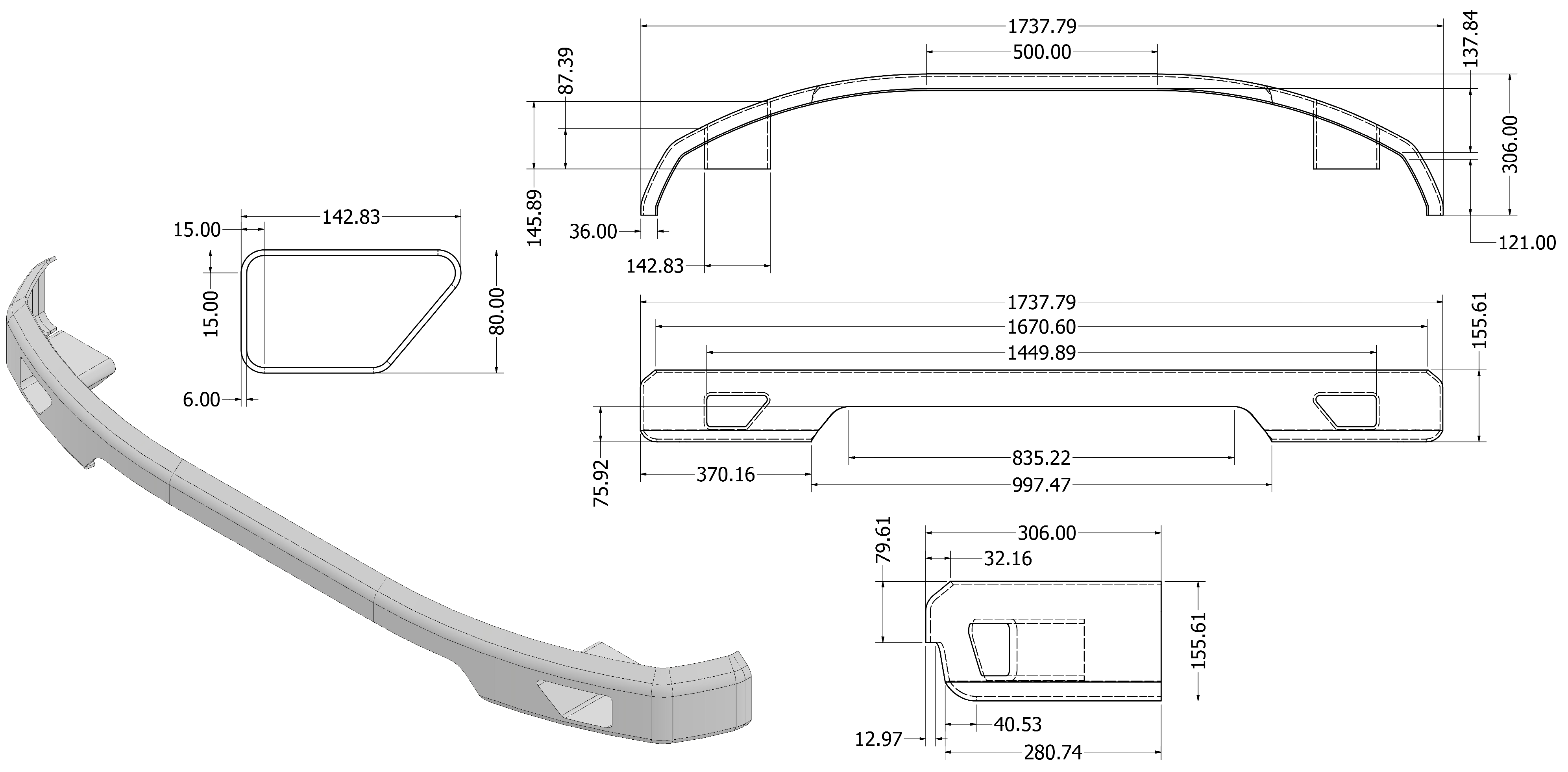
The cross-sectional geometry model significantly affects crashworthiness, the ability to absorb energy, and resistance to deformation in a crash. In addition, the front bumper has a significant function in protecting passengers and minimizing pedestrian injuries [25]. In this study, the simulated front bumper geometry is a hollow cross-section. Closed Hollow models are used to increase strength and ease of integration of towing devices. Figure 1 shows the geometric dimensions of the low bumper type, including bumper height and width, which provide safer pedestrian foot protection. The dominant value of low bumper dimensions in the clearance between the car and the ground reduces the risk of foot injuries [26]. Front Profile front bumpers feature a low, sloped profile. This profile was chosen because it significantly reduces the risk of pedestrian fatalities compared to the high profile. The optimal thickness of the front bumper in this study ranged from 2 to 6 mm, depending on the composite ply thickness.

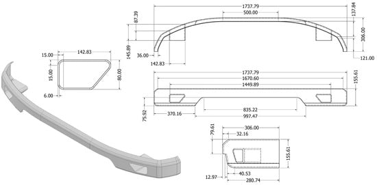
Figure 1. Car bumper design with detailed dimensions (mm).

Autodesk Inventor software is used to create the geometry of front bumper with a surface model. The geometry is exported, and the thickness is defined based on the number of composite laminates using ANSYS ACP. Furthermore, the static structural analysis is performed to assess the reliability of the model’s shear stress and total deformation.

2.2. Assigned Materials

This study critically evaluated the selection of bumper materials, focusing on carbon-fiber-reinforced epoxy and carbon-fiber-reinforced polyamide (CFRP), which demonstrated superior performance. We used the same material as reported by Lotfy et al. [27] and Mahmoud [28], where the 10 properties in Table 1 were adopted from that study. By employing lightweight composites, this study highlights their potential as a promising alternative to conventional metals, improving impact resistance, enabling high-performance automotive design without compromising structural integrity, and supporting improvements in fuel efficiency.

Table 1. Comparison of mechanical properties from previous studies.

Properties	Unidirectional [27]	Woven [27]	CFRP [28]	Unit
Density	1490	1420	1764	kg/m3
Young modulus in X	121,000	61,340	230,000	MPa
Young modulus in Y	8600	61,340	17,900	MPa
Young modulus in Z	8600	6900	17,900	MPa
Poisson ratio in XY	0.27	0.04	0.22	-
Poisson ratio in YZ	0.4	0.3	0.3	-
Poisson ratio in XZ	0.27	0.3	0.22	-
Shear modulus in XY	4700	3300	11,790	MPa
Shear modulus in YZ	3100	2700	6880	MPa
Shear modulus in XZ	4700	2700	11,790	MPa

2.3. Mesh Convergence

The mesh modeling process begins with importing a 3D CAD model into a mesh reconstruction network, which produces a deformation map. This map is used to reshape a predefined template mesh to fit the desired geometry while generating a preliminary low-resolution texture. Following this, the CAD model, deformation map, and low-resolution texture are fed into a texture reconstruction network, which synthesizes a detailed, high-resolution texture [29]. During the training phase, the mesh reconstruction network is refined by comparing its rendered outputs with the ground-truth meshes. The reconstruction loss, calculated by evaluating differences between the rendered object, the predicted mesh, and the annotated ground truth, provides feedback to enhance both the geometric precision and the texture quality of the resulting mesh. In this study, the frame structure was discretized using different body sizes (2–5 mm) at linear element order, resulting in varying numbers of elements.

Figure 2 shows a full-mesh of quadrilateral elements covering the bumper geometry, with a uniform distribution. At a body sizing element size of 2 mm, the mesh is sufficiently fine to capture even subtle curvature and cutout features, resulting in a high total element count and a smooth surface approximation. Notice how the element edges closely conform to the geometry, with minimal distortion, ensuring that critical load paths and stress concentration zones are resolved accurately in subsequent analyses. Meanwhile, the bottom views zoom in on a localized region: on the left, the magnified mesh illustrates consistent element sizing and a clean, orthogonal pattern around a complex cut-out profile, while on the right, the red ellipse highlights a typical quadrilateral patch. Here, each quad element displays nearly equal edge lengths and interior angles close to 90°, a hallmark of good mesh quality that helps avoid numerical stiffness and solution artifacts. The smooth gradation from smaller quads around geometric details to slightly larger quads on flatter areas also demonstrates a well-implemented mesh-sizing strategy that balances accuracy with computational efficiency.

Figure 2. Generated mesh strategy.

2.4. Defining Composite Layers

This study examined five stacking layers composed of carbon–epoxy composites, as illustrated in Figure 3. Each configuration was subjected to two types of orientations, including unidirectional (UD) and woven, and five angles to consistently compare static structural features and specific energy absorption (internal and kinetic) in explicit dynamics. The composite definition was examined for a 6 mm layup comprising six layers, each 1 mm thick. This configuration is relevant to a prior finding conducted by Ren et al. [30] who provided the insight into research on the exact configuration of a bumper for a spacecraft shield application.

Figure 3. Configuration of carbon–epoxy composite specimens (6 mm) in simulation testing.

Figure 3 shows the full range of laminate architectures evaluated in this study, highlighting the influence of fiber orientation and stacking angle. For each layer count, alternating plies were sequentially stacked using either unidirectional or woven reinforcement; single-angle layups (0°, 45°, or 90°) and double-angle configurations (45°/−45° and 0°/90°) were employed to capture variations in in-plane stiffness and interlaminar behavior. By systematically varying the layer angle alongside the fiber architecture, we achieved a specimen that enables a comprehensive assessment of governing mechanical performance, damage initiation, and failure progression.

All simulations were conducted in the ANSYS ACP environment within Mechanical APDL following a structured workflow. Constituent material properties for fiber and matrix phases, such as elastic moduli, Poisson’s ratios, and strengths, were entered into the engineering data module and combined to create orthotropic laminate definitions. The specimen geometry was then imported and assigned a composite section. In ACP, a new layup was created for each test configuration: the total ply count was specified (6 layers), and each layer was defined by its material, thickness (6 mm), orientation angle (0°, ±45°, 90°), and fiber architecture (unidirectional or woven). After confirming the stacking sequence in the layup viewer, the model was discretized using SHELL281 elements (composite option enabled) with mesh controls set to capture expected stress gradients. Boundary conditions were applied to simulate grip and symmetrical constraints, and mechanical loads (forces and displacements) were applied to the appropriate faces. A static structural analysis was specified, and output requests were configured for interlaminar shear stress and failure indices based on the Tsai–Wu criterion (see Section 2.5.3). The analysis was executed, and post-processing in ACP Failure produced a ply-by-ply map of failure initiation. At the same time, global response metrics (deformation and stress distributions) were extracted in Mechanical APDL to evaluate the effects of fiber orientation on laminate performance.

As shown in Figure 4, the outlines a five-stage, parameter-driven workflow in which the ACP (Pre) system defines the composite layup, material properties, and detailed mesh, then passes that exact ply-resolved model into a static structural analysis to impose pre-loads and establish the service-state stress field, and transfers the pre-stressed configuration into a modal analysis to determine the appropriate frequency as the input for harmonic response. At this stage, harmonic response determines a structure’s steady-state response to sinusoidal or harmonic loads over a range of frequencies. Finally, it is connected to the explicit dynamics simulation to capture the high-rate impact response. All five stages draw from a standard parameter set. By leveraging a unified parameter set, we can run a range of loading or boundary condition variables in a single run, automating hundreds of cases and slashing manual setup and overall turnaround time while guaranteeing consistent geometry, mesh, and material definitions across all stages.

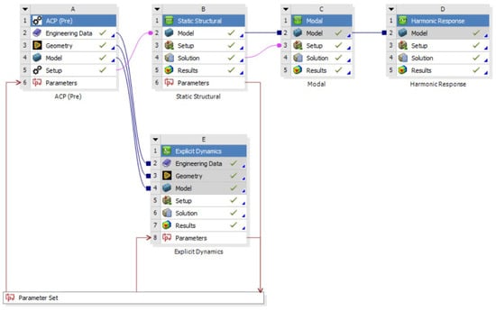
Figure 4. ANSYS workbench simulation flow, blue lines (shared data), pink lines (transfer data).

2.5. Basic Calculations

Through a simulation study, mathematical operations are used to represent real systems in virtual models. However, this methodology has significant limitations, particularly in numerical approaches, due to simplifying assumptions and computational constraints that can introduce numerical errors and reduce accuracy under certain conditions. Therefore, the results should be interpreted with caution, as they depend on the chosen numerical scheme and parameter settings. Below are some approaches, presented as follows.

2.5.1. Linear Elastic Constitutive Model

In numerical simulation, despite its limitations in minimal strains and a limited range of deformation rates [31], linear elasticity is considered one of the valuable and simple approaches in material studies [32]. Therefore, this study clarifies the fundamental assumptions consisting of linearity (proportional stress and strain), perfect elasticity (no permanent deformation), and slight deformation (small displacement and strain). This study uses a theory based on linear anisotropic constitutive relations in the commercial FEM package ANSYS. As shown by Vlach et al. [33], the linear formulation of stress ($\tilde{\sigma }$) and strain ($\epsilon$) are shown by Equations (1) and (2) as follows.

$$\left\{\tilde{\sigma }\right\}=\left[C^0\right].\left\{\epsilon \right\}$$

(1)

$$\left[C^0\right]=\left[\begin{array}{ccccc}{\displaystyle \frac{E_1^0}{1-v_{12}^0{v}_{21}^0}}& {\displaystyle \frac{{v_{21}E}_1^0}{1-v_{12}^0{v}_{21}^0}}& 0& 0& 0\\ {\displaystyle \frac{{v_{12}E}_1^0}{1-v_{12}^0{v}_{21}^0}}& {\displaystyle \frac{E_2^0}{1-v_{12}^0{v}_{21}^0}}& 0& 0& 0\\ 0& 0& G_{12}^0& 0& 0\\ 0& 0& 0& G_{13}^0& 0\\ 0& 0& 0& 0& G_{23}^0\end{array}\right]$$

(2)

where $C^0$ is the initial stiffness matrix of the composite without the damaged effect, $E_1^0$ and $E_2^0$ are the elastic modulus of non-damaged material in specific directions, $v^0$ is Poisson’s ratio of undamaged material, $G_{12}^0$ is the shear modulus of non-damaged material, and $G_{13}^0$ and $G_{23}^0$ are transverse shear modulus of non-damaged material.

To provide a specific case in shear stress, the stress calculation of the damaged composite layer ($\sigma$) is performed using Equations (3) and (4), where $C^d$ represents a stiffness matrix with consolidated damage factor in a specific direction ($d_1$, $d_2$, $d_{12}$, $d_{13}$, and $d_{23}$).

$$\left\{\sigma \right\}=\left[C^d\right].\left\{\epsilon \right\}$$

(3)

$$\left[C^d\right]=\left[\begin{array}{ccccc}{\displaystyle \frac{(1-d_1)E_1^0}{1-(1-d_1)(1-d_2) v_{12}^0{v}_{21}^0}}& {\displaystyle \frac{\left(1-d_1\right)\left(1-d_2\right) v_{21}^0{E}_1^0}{1-(1-d_1)(1-d_2)v_{12}^0{v}_{21}^0}}& 0& 0& 0\\ {\displaystyle \frac{(1-d_1)(1-d_2){v_{12}^{0}E}_2^0}{1-(1-d_1)(1-d_2)v_{12}^0{v}_{21}^0}}& {\displaystyle \frac{(1-d_2)E_2^0}{1-(1-d_1)(1-d_2)v_{12}^0{v}_{21}^0}}& 0& 0& 0\\ 0& 0& (1-d_{12})G_{12}^0& 0& 0\\ 0& 0& 0& {(1-d_{13})G}_{13}^0& 0\\ 0& 0& 0& 0& {(1-d_{23})G}_{23}^0\end{array}\right]$$

(4)

Furthermore, the degree of shear damage can be expressed in Equation (5), where $d_1^{+}$, $d_1^{-}$, $d_2^{+}$, and $d_2^{-}$ represent the rates of damage in tension and pressure, and $d_s$ indicates consolidated shear damage factor.

$$d_s=d_{23}=d_{13}=d_{12}=1-(1-d_1^{+})(1-d_1^{-})(1-d_2^{+})(1-d_2^{-})$$

(5)

With $d_1$, $d_2$ and their relation to the effective shear stress is expressed in Equations (6) and (7) as follows.

$$d_1=\left\{\begin{array}{c}{d}_1^{+}, {\widehat{\sigma }}_{11}\ge 0\\ d_1^{-}, {\widehat{\sigma }}_{11}<0\end{array}\right.$$

(6)

$$d_2=\left\{\begin{array}{c}{d}_2^{+}, {\widehat{\sigma }}_{22}\ge 0\\ d_2^{-}, {\widehat{\sigma }}_{22}<0\end{array}\right.$$

(7)

$\widehat{\sigma }$ is the nonlinear notation. Eventually, both equations calculate stresses using a linear expression that is equivalent to the nonlinear formulation. Therefore, the linear elastic method remains robust for shear-stress analysis in both static and explicit dynamics.

2.5.2. Linear Structural Dynamic Model

In accordance with the linear elastic model, dynamic simulation is used to provide a comprehensive discussion of deformation and shear stress. In particular, for modal analysis and harmonic response, the baseline of the FE dynamic database is defined in terms of the modal matrix, as shown by Menga et al. [34]. The dynamic equilibrium in the frequency domain can be expressed in Equation (8) as follows.

$$\left[-M.{\omega }^2+j\left(\omega C+G\right)+K\right]u\left(\omega \right)=F\left(\omega \right)$$

(8)

where $M$ is the mass matrix, $C$ and $G$ are the structural damping, $K$ is the stiffness matrix, $u$ is the field of displacement, and $F$ is the applied force. Moreover, $u$ is expressed as the linear combination of the eigenvectors, which are associated with the system as shown in Equation (9).

$$u\left(\omega \right)=FRF\left(\omega \right)=\Phi q\left(\omega \right)$$

(9)

According to the frequency response functions (FRFs), the modal matrix ($\Phi$) can be multiplied by the transpose (${\Phi }^T)$ system that becomes Equations (10) and (11).

$$\left[\tilde{R}+j\left(\omega \tilde{C}+\tilde{G}\right)\right]q\left(\omega \right)=\tilde{F}\left(\omega \right)$$

(10)

$$\tilde{R}=\left[-{\Phi }^{T}M\Phi {\omega }^2+{\Phi }^{T}K\Phi \right]=[-I{\omega }^2+\Lambda ]$$

(11)

Therefore, the unitary matrix ($I$), damping matrix ($\tilde{C}$), ($\tilde{G}$), and normalized stiffness matrix ($\Lambda$) are the results of final FRFs, as shown in Equation (12).

$$FRF\left(\omega \right)=\Phi q\left(\omega \right)=\Phi {[\tilde{R}+j\left(\omega \tilde{C}+\tilde{G}\right)]}^{-1}\tilde{F}(\omega )$$

(12)

2.5.3. Tsai–Wu Failure Criterion

To predict the failure of composite materials, the Tsai–Wu criterion uses a quadratic polynomial that accounts for anisotropic material properties in the stress components. The selection of the Tsai–Wu method in numerical simulation is based on its ability to integrate various stress components into a single comprehensive failure index, thereby facilitating the prediction of failure initiation points in composite materials [35]. It combines normal and shear stress into a single scalar index, with coefficients derived from experimental strength parameters. The inclusion of interaction terms (notably F12) allows the criterion to account for the combined effects of different stress components.

However, the empirical determination of these coefficients remains a challenge [36,37] due to the difficulty in determining experimental interactions. To address this issue, integrating FE with a Fortran algorithm within numerical software provides a significant advantage, particularly the ability to analyze damage development in fiber orientation, which can serve as a reference for improving the reliability of composite structures [38]. Based on the observations of Rahimi et al. [39], the Tsai–Wu criterion yielded a lower average error of 13.19% compared to the previous ANSYS approach, which yielded 16%. Thus, the modification provides more accurate and efficient predictions for applications in static structures and impact testing. Generally, the Tsai-Wu failure criterion was expressed by Tsai and Wu [40] and reported by Takács et al. [41] as shown in Equation (13).

$$k={\displaystyle \frac{{\sigma }_1^2}{X_t X_c}}+{\displaystyle \frac{{\sigma }_2^2}{Y_t Y_c}}+{\displaystyle \frac{{\tau }_{12}^2}{S_{12}^2}}+\left({\displaystyle \frac{{\sigma }_1}{X_t}}-{\displaystyle \frac{{\sigma }_1}{X_c}}\right)+\left({\displaystyle \frac{{\sigma }_2}{Y_t}}-{\displaystyle \frac{{\sigma }_2}{Y_c}}\right)+{\displaystyle \frac{2F_{12}^{*}{\sigma }_1{\sigma }_2}{\sqrt{X_t{X}_c{Y}_t{Y}_c}}}$$

(13)

* At failure boundary ($FI$) = 1.0.

$X_t$ and $Y_t$ denote tensile strengths in the $x_1$ (fiber-oriented) and $x_2$ (fiber-perpendicular) directions, $X_c$ and $Y_c$ the corresponding compressive strengths, and $S_{12}$ the shear strength in the $x_1-x_2$ plane. The sixth quantity, the interaction coefficient, is written as $F_{12}^{*}$. Hence, the Tsai–Wu parameter vector can be written as $\theta =[X_t, X_c, Y_t, Y_c, S_{12}, F_{12}^{*}]$.

Each stress can be assumed to be factored by the strength ratio ($SR$) to achieve the failure boundary, which is expressed in Equation (14).

$$0.0=\left[{\displaystyle \frac{{\sigma }_1^2}{X_t X_c}}\right.+{\displaystyle \frac{{\sigma }_2^2}{Y_t Y_c}}+2F_{12}^{*}{\sigma }_1{\sigma }_2+\left.{\displaystyle \frac{{\tau }_{12}^2}{S_{12}^2}}\right]{SR}^2+\left[{\sigma }_1\left[{\displaystyle \frac{1}{X_t }}-{\displaystyle \frac{1}{X_C }}\right]+{\sigma }_2\left[{\displaystyle \frac{1}{Y_t }}-{\displaystyle \frac{1}{Y_C }}\right]\right]SR-1.0$$

(14)

Currently, the quadratic equation in SR uses linear scaling for each stress term, so it can be used directly to achieve the desired stress level. Mathematically, these criteria are represented by a second-order (quadratic) polynomial in the stress or strain components into a single scalar expression. Note that the coefficient $F_{12}$ cannot be inferred directly from uniaxial failure stresses; to obtain reliable values, it should be measured under biaxial loading. In practical use, it is typically reported as a dimensionless interaction parameter in Equation (15).

$$F_{12}^{*}={\displaystyle \frac{F_{12}}{\sqrt{\left(F_{11}{F}_{22}\right)}}}$$

(15)

where $F_{11}$ and $F_{22}$ can be expressed as Equations (16) and (17).

$$F_{11}={\displaystyle \frac{1}{X_t X_c}}$$

(16)

$$F_{22}={\displaystyle \frac{1}{Y_t Y_c}}$$

(17)

To guarantee that the failure surface is a closed cone, the coefficient $F_{12}^{*}$ must lie inside a prescribed interval of −1 < $F_{12}^{*}$ < 1; in practice, the admissible interval that produces physically realistic behavior is even narrower. A commonly adopted value of ½ from this family makes the generalized von Mises form. Since the von Mises stress is not applicable for anisotropic material, the Tsai–Wu constant reduces to −1. Therefore, Equation (13) can be transformed into Equation (18), yielding the Tsai–Wu 3D expression.

$$\begin{gathered} k={\displaystyle \frac{-{\sigma }_1^2}{X_t X_c}}-{\displaystyle \frac{{\sigma }_2^2}{Y_t Y_c}}-{\displaystyle \frac{{\sigma }_3^2}{Z_t Z_c}}+{\displaystyle \frac{{\tau }_{12}^2}{S_{xy}^2}}+{\displaystyle \frac{{\tau }_{13}^2}{S_{xz}^2}}+{\displaystyle \frac{{\tau }_{23}^2}{S_{yz}^2}}-1.0{\displaystyle \frac{{\sigma }_1{\sigma }_2}{\sqrt{X_t{X}_c{Y}_t{Y}_c}}}-1.0{\displaystyle \frac{{\sigma }_2{\sigma }_3}{\sqrt{Y_t{Y}_c{Z}_t{Z}_c}}} \\ \hspace{1em}-1.0{\displaystyle \frac{{\sigma }_1{\sigma }_3}{\sqrt{X_t{X}_c{Z}_t{Z}_c}}}+{\sigma }_1\left({\displaystyle \frac{1}{X_t}}-{\displaystyle \frac{1}{X_c}}\right)+{\sigma }_2\left({\displaystyle \frac{1}{Y_t}}-{\displaystyle \frac{1}{Y_c}}\right)+{\sigma }_3\left({\displaystyle \frac{1}{Z_t}}-{\displaystyle \frac{1}{Z_c}}\right) \end{gathered}$$

(18)

In software simulation, the other interaction terms may be treated in the same manner as

• XY = $2F_{12}$;
• XZ = $2F_{13}$;
• YZ = $2F_{23}$.

2.6. Bumper Impact Test Through Static Structural and Explicit Dynamics

To perform the bumper impact test, we employ both static structural analysis and explicit dynamics as complementary tools. The static model establishes baseline stiffness and deflection under static (stable) conditions, while the explicit dynamics model then captures the full transient (dynamic) event under prescribed impact velocities. Both analyses share the same geometry, layups, and material properties, and their outputs include total deformation, shear stress, and failure indices, providing a consistent framework for assessing crashworthiness.

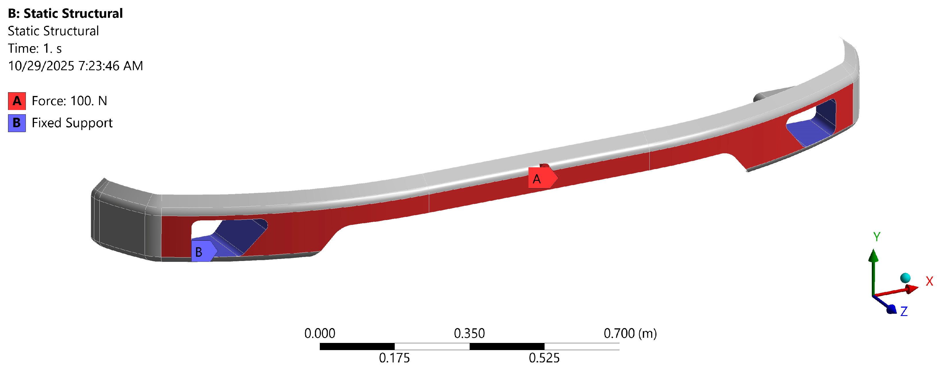
For static structural simulation on the front bumper, the boundary condition is first defined (see Figure 5). The boundary condition definition is performed in two stages, particularly the fixed support and load definition. In the simulation, the fix support is defined on the right and left intake ducts, which correspond to the car bumper holder, while the load is applied as a force at the front cross-sectional surface. The static force acts on the front cross-section with a force of 100 Newtons. It is essential to know how responsive and elastic the bumper is before receiving a large load [42]. These force tests are used to measure shear stress. These data are essential for designing bumpers that can absorb impact energy without immediate damage.

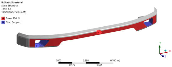
Figure 5. Boundary condition of the static structural test.

On the other hand, impact testing is a test method used to assess the resistance and performance of a structure or component to impact loads. The test procedure typically involves applying an impact load of a specified energy, velocity, or force to the test object and then measuring the response, such as deformation, stress, or damage, to ensure that the component meets safety and functionality requirements [43]. Explicit dynamics simulation can be used to predict design failures using impact test schemes. Explicit dynamics is a finite element-based numerical method for analyzing the response of structures to very fast dynamic loads, such as impact or explosion, accounting for material nonlinearity, contact, and large deformations. In these simulations, time is divided into small steps, and solutions are calculated explicitly at each step, making them particularly suitable for short-duration events and extreme changes in conditions [44]. These simulations enable detailed predictions of structural behavior without the need for repeated physical tests, thereby speeding up the design and optimization process and reducing development costs.

Impact simulation using explicit dynamics for a car front bumper begins by modeling the bumper’s geometry and related components in Autodesk Inventor and then importing them into ANSYS for preprocessing. Next, the contact between the bumper and the collision object is defined in Figure 6. The contact surface is defined as a rigid wall by specifying the relevant materials. The main boundary conditions that need to be set include fixation of the bumper mounting points by locking translation and rotation in the area and defining the velocity or impact force on the bumper surface according to the frontal impact scenario [45]. Velocity varies in three speeds based on NHTSA Tests [46]: Code TC 1.1.3 with a velocity of 80 km/h = 22.222 m/s, code TC 1.1.2 with a velocity of 56.2 km/h = 15.611 m/s, and code TC 1.1.1 with a velocity of 40 km/h = 11.111 m/s. After that, mesh with element sizes ranging from 6 mm to 10, and then calculate the mesh convergence rate to obtain accurate results in the minimum time. The selection of a mesh size of 6–11 mm is recommended for structural analysis, which requires a balance between detailed results and computation time, with further customization based on the specific needs of the geometry [47].

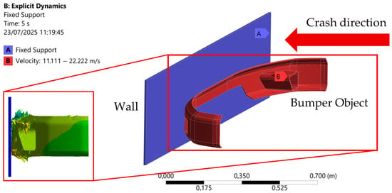
Figure 6. Boundary condition of explicit dynamics test.

To ensure transparency and reproducibility of the workflow, the finite-element input parameters are summarized in Table 2. This table clarifies the simulation process for both the static structural and explicit dynamics analyses.

Table 2. Finite element analysis (FEA) parameters input.

Properties	Value	Unit
Load definition	100	Newton
Number of plies	6	-
Angle alignment	0, 45, 90, 45/−45, 0/90	-
Thickness of each layer	1	mm
Body sizing	2–5 mm	mm
Bumper material	Carbon–epoxy, CFRP	-
Wall material	Structural steel	-
Meshing method	Quadrilateral dominant	-
Failure mechanism	Tsai–Wu	-
Carbon–epoxy volume fraction	0–100%	-
Controlled speeds	11.11, 15.61, 22.22	m/s
End time	10	s
Maximum number of cycles	500,000	-
Reference energy cycle	6000	-

The analysis of explicit dynamics simulation results for automobile front bumpers focuses on several key parameters, including deformation, energy absorption, stress distribution, and impact acceleration. This simulation allows real-time visualization of the structure’s deformation during impact, enabling identification of the most severely damaged areas and how the bumper material absorbs the impact energy. The simulation results show the average deformation value and maximum shear stress, which are crucial for assessing the effectiveness of the design in protecting the components behind it [48]. In addition, analyzing internal and kinetic energy helps evaluate how much impact energy is effectively absorbed by the bumper, which is directly related to crashworthiness. The simulation results also compare the design performance at various speeds, further supporting the design. Thus, the analysis of explicit dynamics simulation results provides a comprehensive picture of structural behavior during impact and serves as an essential tool in developing vehicle safety systems.

2.7. Machine Learning-Driven Analysis

Machine learning (ML) has emerged as a powerful approach to this problem, offering feature selection, enhanced predictive performance, validation of results, greater computational efficiency, and improved model interpretability and data quality.

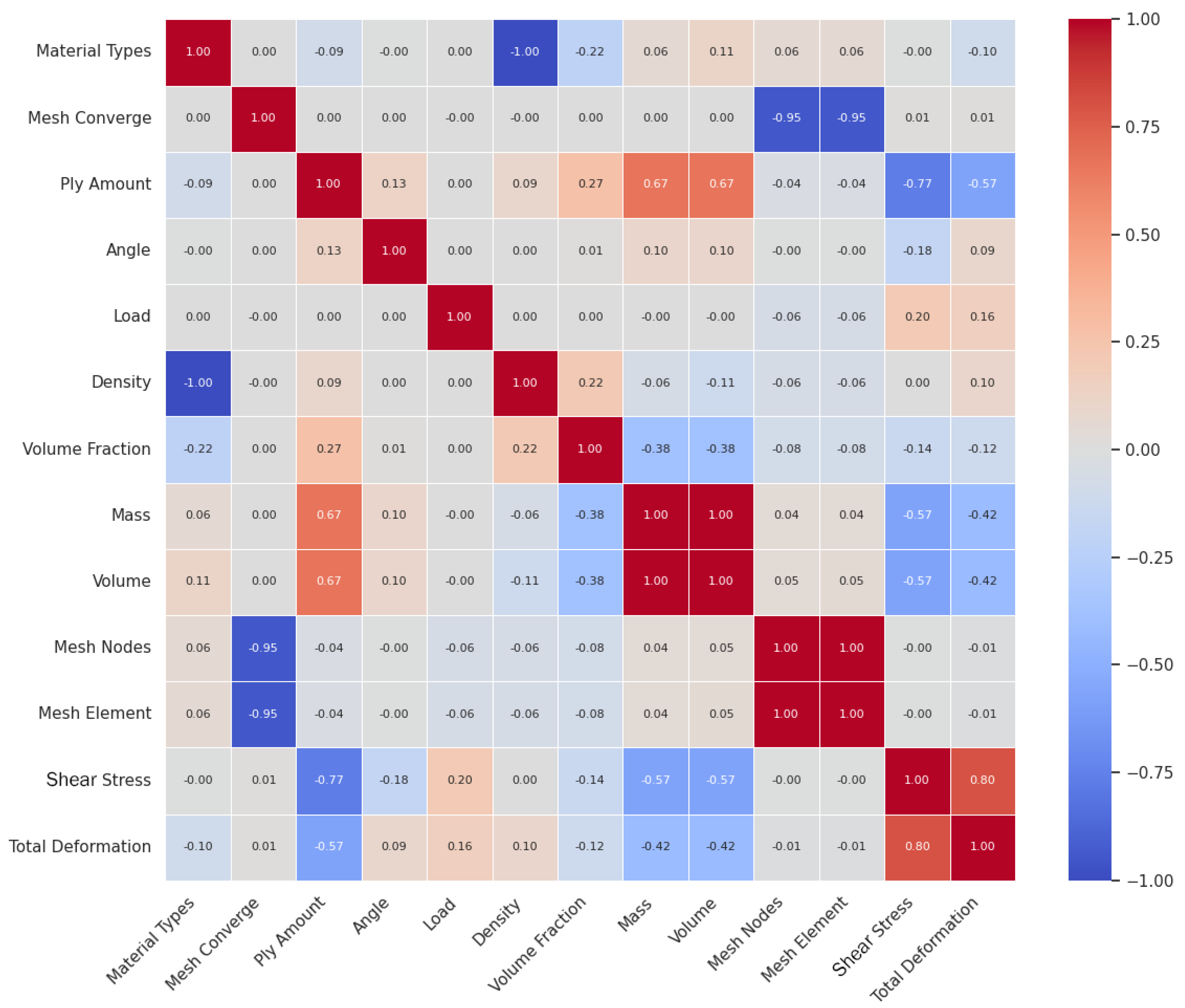
A supervised machine learning approach was employed to forecast and assess the normality of ANSYS simulation results. The model was trained on a dataset consisting of 11 variables (see Figure 7), designated as input features, and two parameters (shear stress and total deformation) as prediction targets, with a size of 13 × 1450. Here, features consist of standardized data points that share a common coordinate framework and inform the model, while targets represent the specific outcomes the research aims to predict. The workflow followed a typical machine learning pipeline: beginning with data preprocessing and exploratory data analysis, proceeding to model training and evaluation, and concluding with results visualization. Since our dataset contains multiple targets, we performed multivariate analysis on various performance targets.

Figure 7. Heatmap correlation of features.

We quantified inter-variable associations using a correlation matrix in Figure 7. Correlation coefficients range from −1 to +1, where positive (“+”) values indicate a direct relationship (both variables tend to increase or decrease together) and negative (“−”) values indicate an inverse relationship (one increases as the other decreases). The magnitude (|r|) reflects strength (0 weak, ≥0.5 moderate, ≥0.7 strong), whereas the sign reflects direction, but the correlation does not imply causation.

2.7.1. Data Preprocessing

Data preprocessing is a critical step that readies the dataset for effective learning by removing irrelevant variables, converting data types, handling missing values, and performing column and row cleaning, feature coding, and data normalization [49]. In our dataset, load and safety factor each had 18 missing entries, while speed, internal energy, and kinetic energy were missing in 1430 out of 1450 cases. Because the latter three variables had more than 98% missingness and were only applicable in specialized scenarios, we dropped them entirely. For load and safety factors under 1.3%, we applied median imputation. After these actions, we performed multivariate validation by inspecting pairwise correlations to uncover unexpected dependencies, applying outlier detection to flag anomalous observations, and checking distributional consistency across subgroups. These steps ensure that the remaining features are complete, coherent, and representative before model training.

2.7.2. Exploratory Data Analysis

EDA is an essential step in the data analysis process that uses statistical and visualization techniques to examine datasets, discover patterns, find anomalies, test hypotheses, and check assumptions [50]. Features and targets constitute the core elements of the dataset, which captures how multiple variables influence the mechanical performance. This dataset, generated from simulation studies conducted in all ANSYS simulations, includes 12 input features (material types, mesh convergence, ply amount, angle, load, speed, density, volume fraction, mass, volume, mesh nodes, mesh element), and five response variables (shear stress, total deformation, safety factor, internal energy, kinetic energy). Exploratory data analysis (EDA) plays a critical role, employing statistical summaries, and graphical techniques to reveal underlying patterns, detect outliers, validate assumptions, and guide hypothesis testing [51].

The statistical profile of our dataset consists of 1450 numbers, reporting for each variable its meaning, standard deviation, and key percentiles (0%, 5%, 50%, 95%, and 100%). The first six entries (material type, mesh convergence, ply count, fiber angle, applied load, and density) characterize the composite geometry and boundary conditions. Volume fraction, mass, and the overall component volume are shown, along with mesh resolution metrics (total nodes and elements). Furthermore, the 11 selected features (except speed) and two impactful targets (shear stress and total deformation) quantify the primary structural responses under quasistatic loading. Therefore, we have excluded some variables, such as speed, safety factors, internal energy, and kinetic energy, from further analysis because each had over 50% missing values and appeared only in specific subsets rather than consistently across all simulation scenarios.

2.7.3. Multivariate Analysis

Multivariate analysis is a statistical technique that simultaneously evaluates several outcome measures, such as various adverse events, while accounting for multiple predictors in one comprehensive model, enabling unbiased and precise estimation of each parameter [52]. Multivariate analysis is a statistical technique that simultaneously evaluates several outcome measures, such as adverse events, while accounting for multiple predictors in a comprehensive model, enabling unbiased and precise estimation of each parameter. To verify the assumptions underlying this approach, we examine the distributions of each response variable using histograms and quantile–quantile (Q–Q) plots: histograms reveal the empirical frequency distribution of each outcome, while Q–Q plots compare observed quantiles with those of a theoretical normal distribution. Together, these graphical diagnostics confirm whether the multivariate targets satisfy the normality assumption required for valid inference and guide any necessary transformations before modeling fitting.

2.7.4. Train–Test and Model Evaluation

The model’s performance was evaluated using mean squared error (MSE) and the coefficient of determination (R²). This research demonstrated various regression techniques. Chicco et al. [53] defined their metrics using MSE and R² to assess regression accuracy. This concise report focuses solely on R² to measure predictive quality. MSE represents the average squared difference between predicted and actual values that is accounted for by the independent variables, as defined in Equation (19).

$$MSE= {\displaystyle \frac{1}{m}}{\sum }_{i=1}^m{\left(X_i-Y_i\right)}^2$$

(19)

In essence, R² quantifies the fraction of variability in the dependent variable that is accounted for by the independent variables, as defined in Equation (20).

$$R^2=1-{\displaystyle \frac{{\sum }_{i=1}^m{(X_i-Y_i)}^2}{{\sum }_{i=1}^m{(\overline{Y}-Y_i)}^2}}$$

(20)

(Desired value: MSE = 0, R² = 1, closer is better.)

In this expression, X_i and Y_i represent the observed and predicted values of the response variable for the i-th sample, respectively. It is common practice to allocate 80% of the data for model training and reserve the remaining 20% for testing, which helps visualize and evaluate model performance.

Python (version 3.12.12) scripts were implemented to enable fast, reproducible prediction and assessment across a suite of regression algorithms tailored to our tabular dataset. Four primary models, (1) linear regression as an interpretable baseline establishing a lower bound and quantifying linear trends; (2) Random Forest for capturing nonlinearities and high-order interactions with built-in out-of-bag validation and feature importance; (3) support vector regressor (SVR) to handle small-to-moderate samples in high-dimensional spaces via kernel mappings and margin maximization; and (4) k-nearest neighbors (KNN) as a nonparametric local learner that exploits neighborhood structure without assuming a global functional form. This mix was chosen to balance bias–variance trade-offs, perform nonparametric behaviors, and probe model stability under distributional shifts. The Python pipeline standardizes preprocessing, cross-validation, and hyperparameter search, ensuring methodical comparisons while preserving traceability and ease of replication.

3. Results and Discussion

3.1. Effect of Single- and Double-Angle Layers on Shear Stress

Building on our selection of six composite layers with a default mesh at a specific thickness (6 mm) as the baseline for its proven convergence and computational efficiency, we present the first investigation of off-axis fiber orientations. In this section, we conduct a systematic comparison between single-angle (0°, 45°, or 90°) and double-angle (45°/−45° and 0°/90°) laminate sequences. We continue to include the UD and woven layups. By retaining these baseline composites, we can more clearly quantify the benefits of off-axis fiber orientations in redistributing loads and reducing peak shear stresses relative to established UD and woven architectures in the crash test. This analysis will inform trade-offs between manufacturing simplicity and mechanical performance, guiding the selection of optimal laminate architectures for applications that demand balanced strength and stiffness.

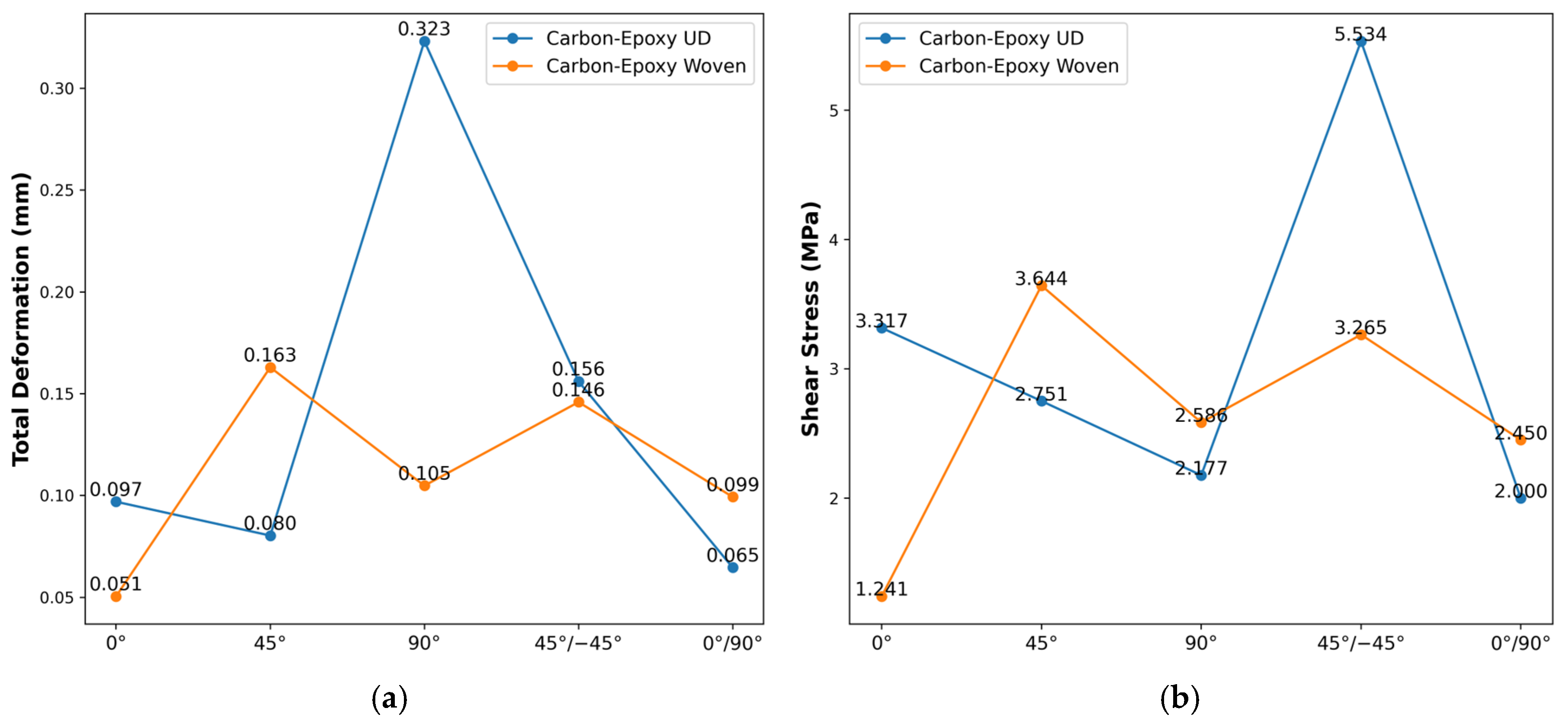
In Figure 8a, UD laminates exhibit their lowest deformation at 0°/90° orientation, reflecting the lowest axial stiffness of fibers oriented perpendicular to the load. As the fiber angle approaches 45°, deformation initially increases slightly to 0.080 mm for the UD orientation, before peaking at 90° to 0.323 mm. By contrast, the lowest deformation in woven was observed at 0° orientation, with a value of 0.051 mm, and a peak of 0.163 mm was observed at 45° orientation, where shear loads produce the highest stress concentration. At the highest point, the UD laminate shows a more pronounced peak than the woven due to its unidirectional nature, accentuating shear-driven stress peaks at off-axis angles. In contrast, the woven fabric’s crisscross architecture moderates these spikes. As a result, the 0°/90° orientation (quasi-isotropic laminate) returns to intermediate stress levels, with values of 0.099 mm and 0.065 mm for UD and woven, respectively.

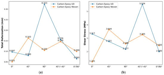
Figure 8. Static structural tests between various layer angle configurations on different materials at 100 N; (a) total deformation (average), (b) shear stress (maximum).

Under the shear-stress examination (see Figure 8b), the almost identical trends are amplified: the UD 45°/−45° laminate reaches the highest stress (5.534 MPa), a 59% jump over its 0° value, while the woven 45°/−45° stack peaks at a more modest 3.265 MPa. The pure transverse (90°) case remains the lowest for UD materials (2.177 MPa), and the 0° orientation shows a 3.317 MPa stress in UD versus only 1.241 MPa in the woven. The larger load accentuates the UD laminate’s sensitivity to off-axis shear, driving its stress further above that of the woven counterpart, whose bidirectional laminate paths continue to smooth stress gradients. This comparison underscores how fiber orientation complexity and fabric architecture jointly influence stress magnitudes at higher loading levels.

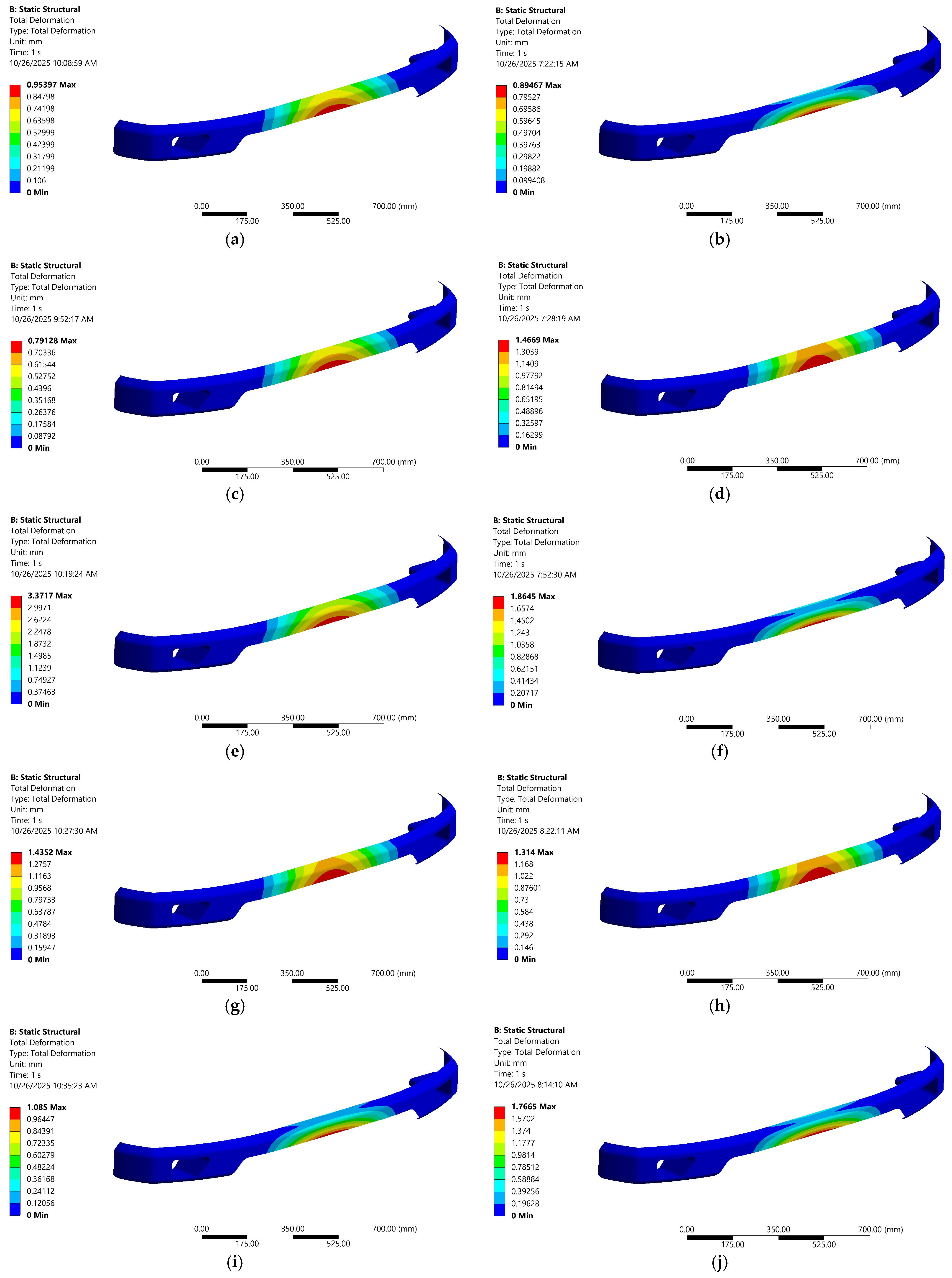
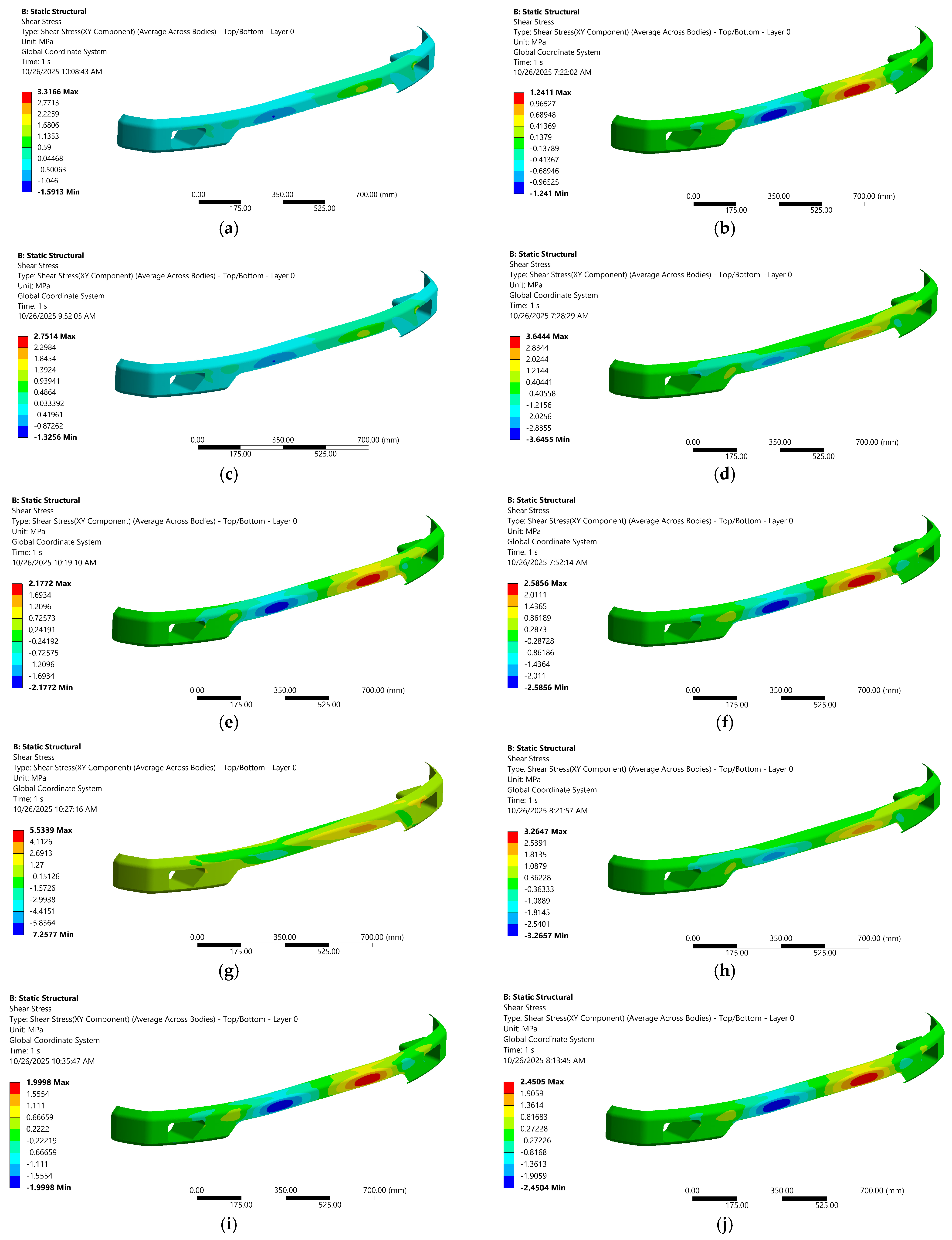
To further clarify the fiber architecture under static load, the contour visualizations of deformation and shear stress are shown in Figure 9 and Figure 10, respectively. Those contours indicate an effective stiffness–compliance trade-off and efficient load transfer. Focusing on comparative deformation and stress contours (see Figure 9b and Figure 10b), the woven carbon–epoxy composite at 0° angle clearly offers the most balanced performance, combining low shear stress, stable web convergence, and enhanced damage tolerance by representing deformation. Moreover, this is reinforced by the statement of Amir et al. [54], who revealed that woven fibers with an orientation of α = 0° are a good alternative compared to 45° and 90° orientations, and the anisotropic materials are better for applications that need strength or other properties in a specific direction [55]. Therefore, the authors decided to continue using woven carbon–epoxy composites oriented at 0° for all subsequent design analysis and optimization in the next section.

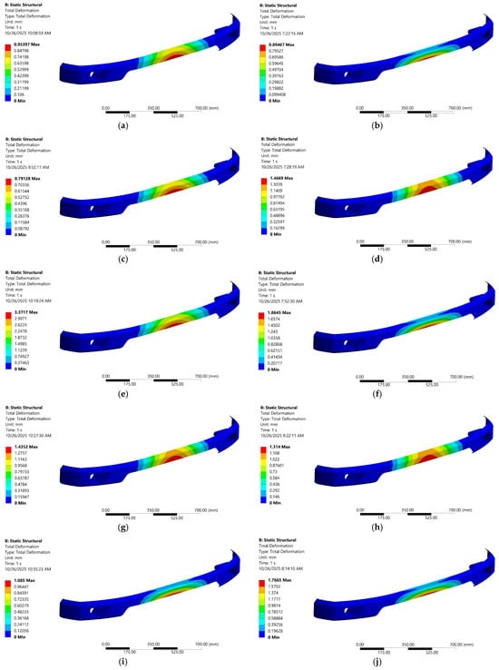
Figure 9. Deformation contour at different angles and architecture; (a) UD—0°, (b) woven—0°, (c) UD—45°, (d) woven—45°, (e) UD—90°, (f) woven—90°, (g) UD—45°/−45°, (h) woven—45°/−45°, (i) UD—0°/90°, (j) woven—0°/90°.

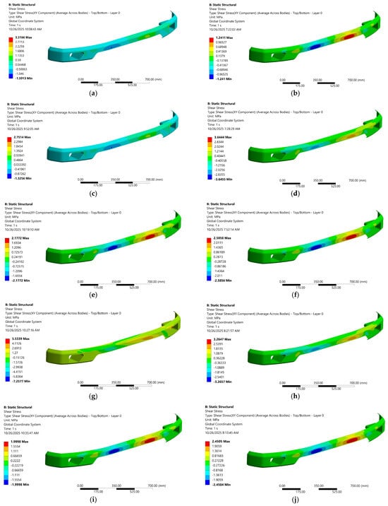
Figure 10. Shear-stress contour at different angles and architecture; (a) UD—0°, (b) woven—0°, (c) UD—45°, (d) woven—45°, (e) UD—90°, (f) woven—90°, (g) UD—45°/−45°, (h) woven—45°/−45°, (i) UD—0°/90°, (j) woven—0°/90°.

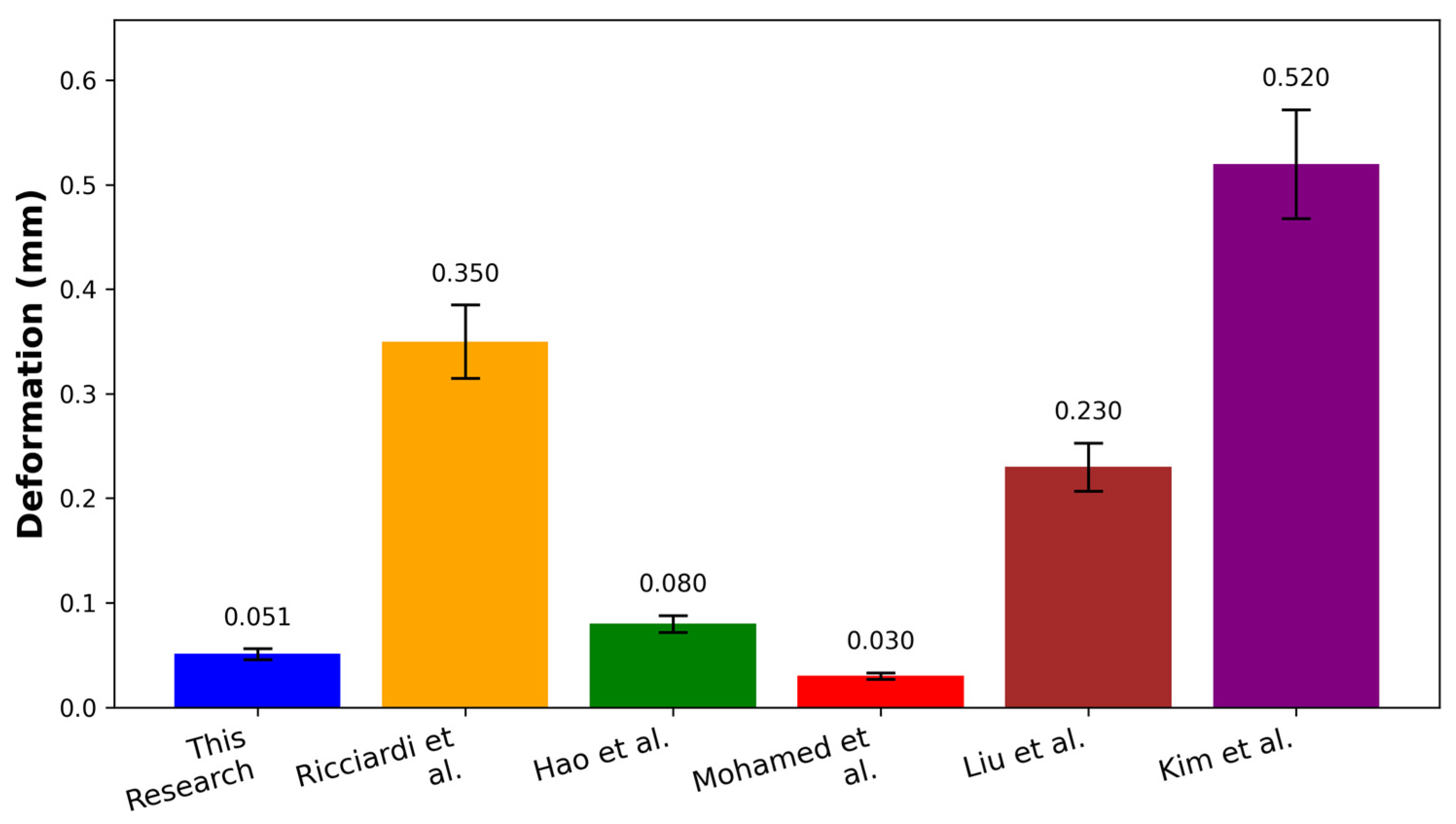
In order to strengthen the analysis and discussion, quantitative benchmarking (see Figure 11) was conducted toward similar studies that justify the deformation of carbon–epoxy composites at 100 N loading and unidirectional configurations based on the findings in Figure 8. Under the prescribed static load, the 0° woven carbon/epoxy laminate used in this work exhibits a deformation of 0.051 mm, which is substantially lower than values reported by Ricciardi et al. [56] (0.350 mm), Hao et al. [57] (0.080 mm), Liu et al. [58] (0.230 mm), and Kim et al. [59] (0.520 mm), while remaining above Mohamed et al. [60] (0.030 mm). This placement at the lower end of the literature range is consistent with the deformation and shear-stress contours, which show efficient load transfer and suppressed shear localization for the 0° architecture.

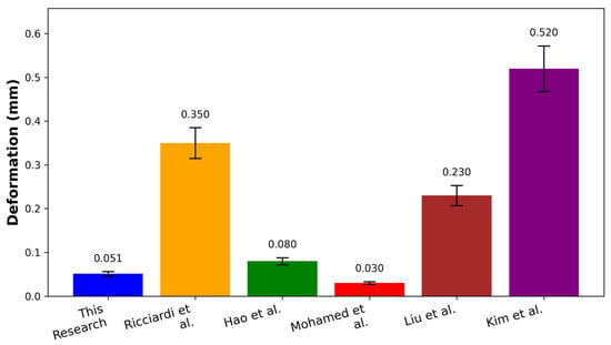
Figure 11. Comparison of our deformation results with some of the research literature at a load of 100 N.

3.2. Optimum Mesh Configuration for Convergent Simulation

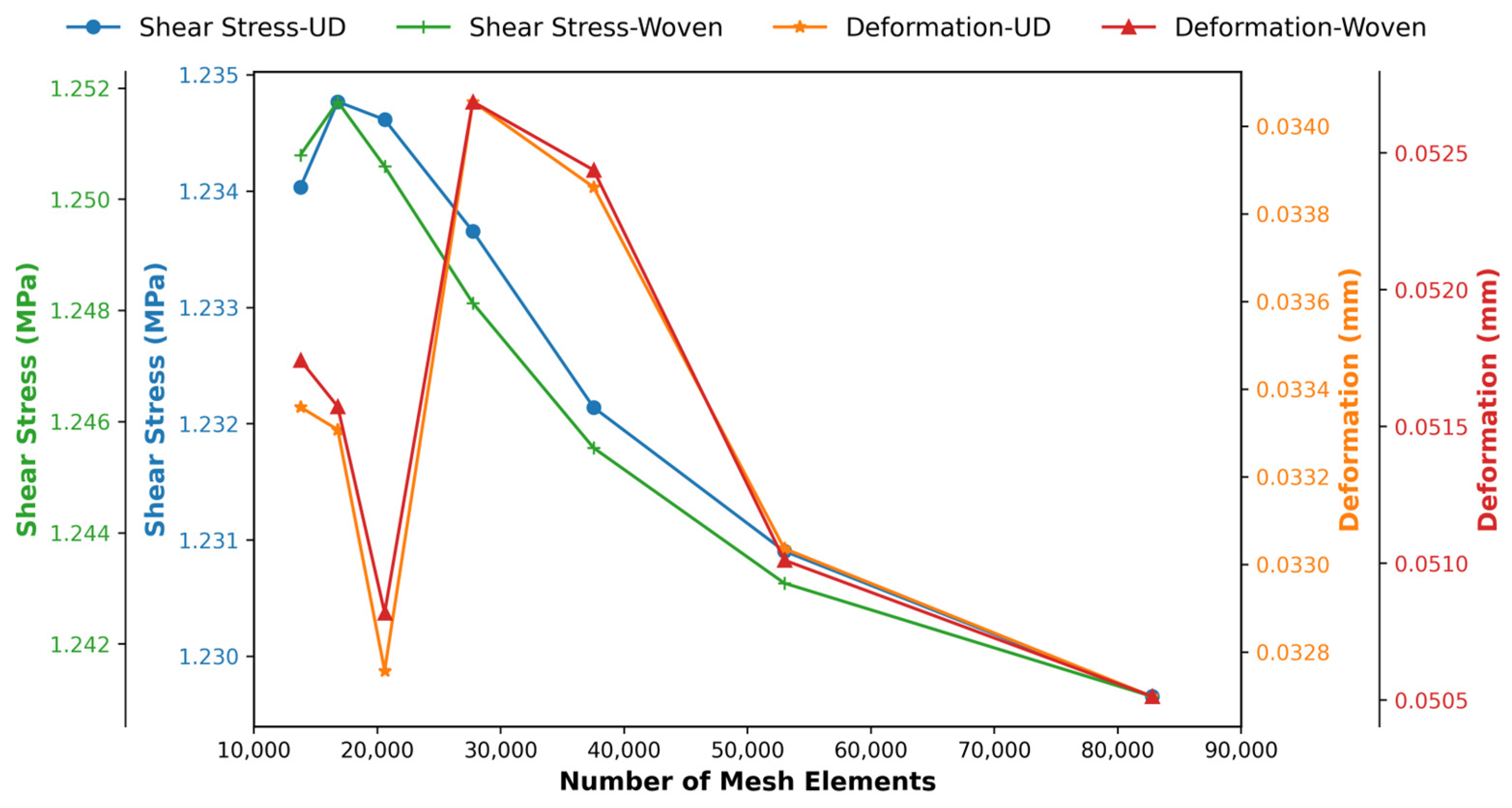
To ensure that the simulation results were not significantly affected by mesh density or overly high computational costs, a mesh independence study was conducted. We investigate how varying the number of mesh elements influences the shear-stress distributions under different mesh densities to ensure solution convergence. Specimens with six plies were modeled using a sequence of quadrilateral meshes from coarse to fine and subjected to identical loading and boundary conditions. A controlled mesh configuration (2–5 mm) was initially applied. Furthermore, Table 3 and Figure 12 are presented to show a good correlation between mesh count and maximum shear stress.

Table 3. Mesh configuration profile against generated mesh elements.

Body Sizing (mm)	Mesh Nodes	Mesh Element
2	83,664	82,793
2.5	53,755	52,978
3	38,164	37,525
3.5	28,302	27,739
4	21,077	20,597
4.5	17,237	16,794
5	14,149	13,769

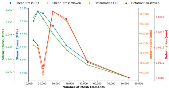
Figure 12. Mesh convergence in various body sizing on 6 laminates at 0° orientation.

Table 3 illustrates the inverse relationship between the body sizing element size (mm) and the number of generated mesh features in a mesh or finite element model. As the body sizing element size increases from 2.0 mm to 5.0 mm, the number of generated nodes and elements significantly decreases. The mesh size directly influences both the accuracy of the simulation results and the total number of generated mesh features during the meshing process [61]. This trend reflects a typical meshing behavior in computational modeling: smaller element sizes lead to a finer mesh and, consequently, a higher number of nodes and elements, improving accuracy but increasing computational cost. Conversely, larger element sizes reduce the mesh density, lowering computational demand but potentially compromising result precision.

As mesh refinement progressed (see Figure 12), peak shear stresses converged toward stable values. This trend shows a clear net convergence trend for shear stress. As the number of mesh elements increases, the calculated shear stress decreases slowly and steadily, indicating that the solution approaches mesh independence with mesh refinement. On the other hand, the deformation history is more volatile. It reduces on refinement from coarse to medium, shows a striking peak at medium mesh density, and then decreases again with further refinement. This behavior is consistent with the web’s sensitive capture of local gradients and stress concentrations, where medium webs may inadvertently align element boundaries with high-stress regions, resulting in interpolation/locking, or inadequately integrate curvature and boundary conditions, all of which temporarily amplify predicted displacements.

The relationship between the two responses is not strictly linear: globally, the two quantities converge in a downward direction as the mesh fidelity increases (overall negative trend), but locally, the intermediate deformation peaks coincide with small perturbations in the shear stress, suggesting a short-range positive coupling when local discretization errors amplify both strain and stress measures; once the mesh is sufficiently refined, this discretization-induced correlation disappears and the fields separate towards the proper solution. Overall, the largest mesh is the most justifiable choice for reporting physical results: it produces the least deformations, the most stable shear stresses, and therefore the strongest numerical evidence of convergence. Despite the higher computational cost, it is the best choice for reliable, publication-quality results.

Based on these convergence studies, a 0° configuration woven on a 2 mm mesh with six layers emerged as the optimal compromise between accuracy and computational efficiency. By selecting that for all subsequent investigations, the authors ensured that peak shear stresses were resolved with high fidelity without incurring excessive solution times associated with finer discretization. This choice provides a solid foundation for more in-depth parametric studies and design optimization of composite structures.

3.3. Investigation of Volume Fraction in Carbon Composite Combinations

Having established a 0° woven carbon–epoxy laminate at 2 mm mesh as the base material, we now turn to optimizing its layer ratio to maximize mechanical performance by combining it with other materials. This section investigates how varying the carbon–epoxy laminate fraction, from 20% to 100%, affects deformation and shear stress. Through a combination of micromechanical modeling and finite element simulations at each volume fraction, we aim to investigate the effect of incorporating additional substrates and quantify their optimal proportions, ensuring the selected configuration meets the structural and manufacturing constraints for advanced composite applications. To elucidate the impact of combining additional materials with woven reinforcement on the mechanical response of hybrid composites, this study combines a 6 mm woven carbon–epoxy fabric with carbon-fiber-reinforced polyamide (CFRP) layers in various proportions. At 100% a pure woven laminate is indicated, while 80% indicates that four-fifths of the total reinforcement layer is woven fabric, and only the remaining 20% is CFRP material. Thus, the lower percentage reflects a decrease in the volume fraction of the woven component and a compensatory increase in the CFRP fraction.

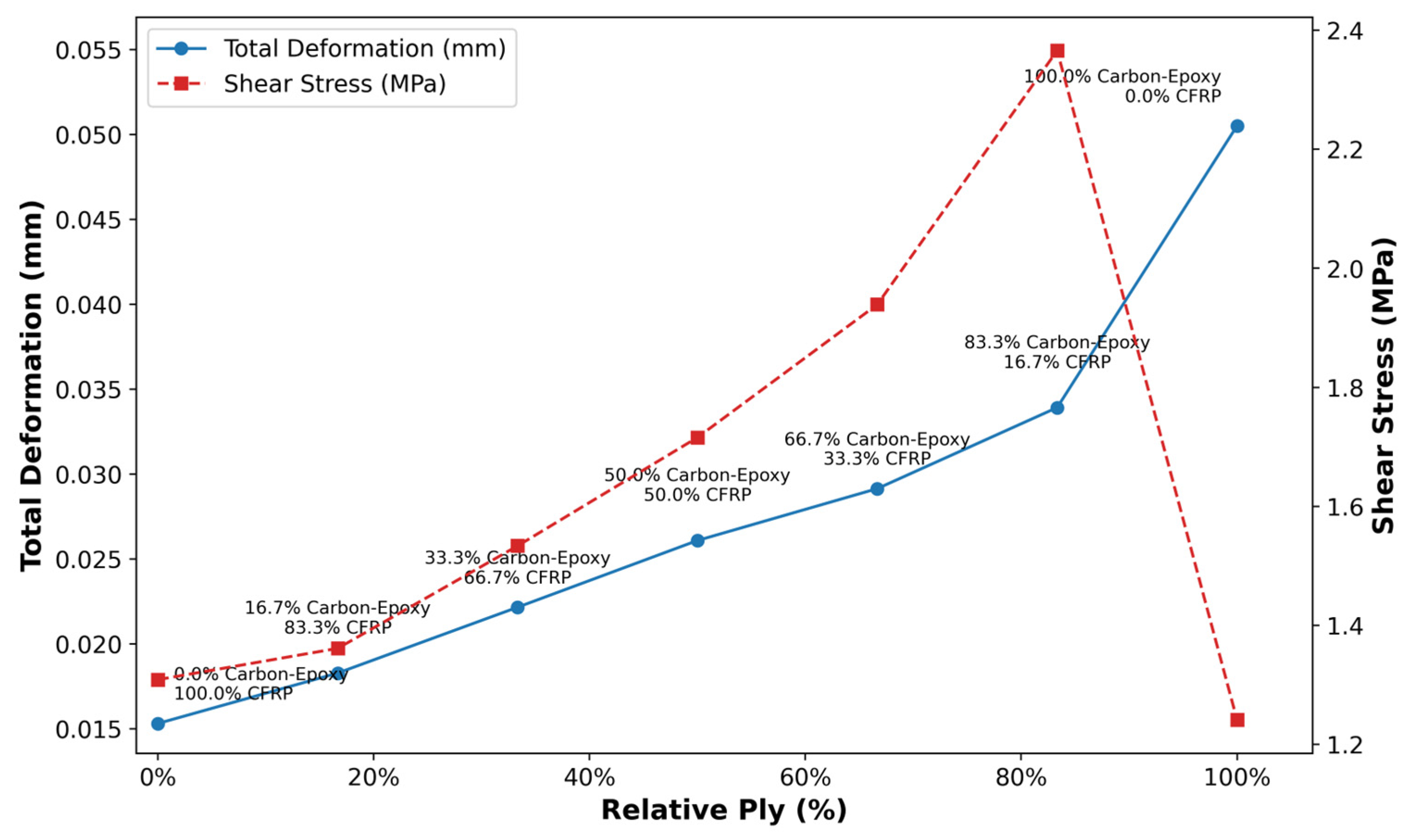
Figure 13 summarizes the mechanical response as the relative fraction of carbon–epoxy plies increases (replacing the baseline CFRP plies). Total deformation rises steeply from 0.015 mm at 0% carbon–epoxy to 0.051 mm at 100%, indicating a steady reduction in global bending stiffness with increasing CFRP content. In contrast, the shear-stress response is non-monotonic, rising from 1.3 MPa at 0% to a clear maximum of 2.36 MPa at 83.3% carbon–epoxy, then dropping abruptly to 1.25 MPa at 100%. Thus, while compliance increases continuously with carbon–epoxy fraction, peak shear stress is highest in hybrid laminates just shy of full carbon–epoxy substitution.

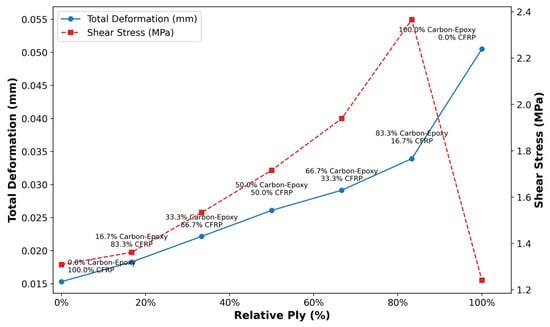
Figure 13. Effect of the fraction between carbon–epoxy and carbon-fiber-reinforced polyamide on shear stress and deformation at 100 N.

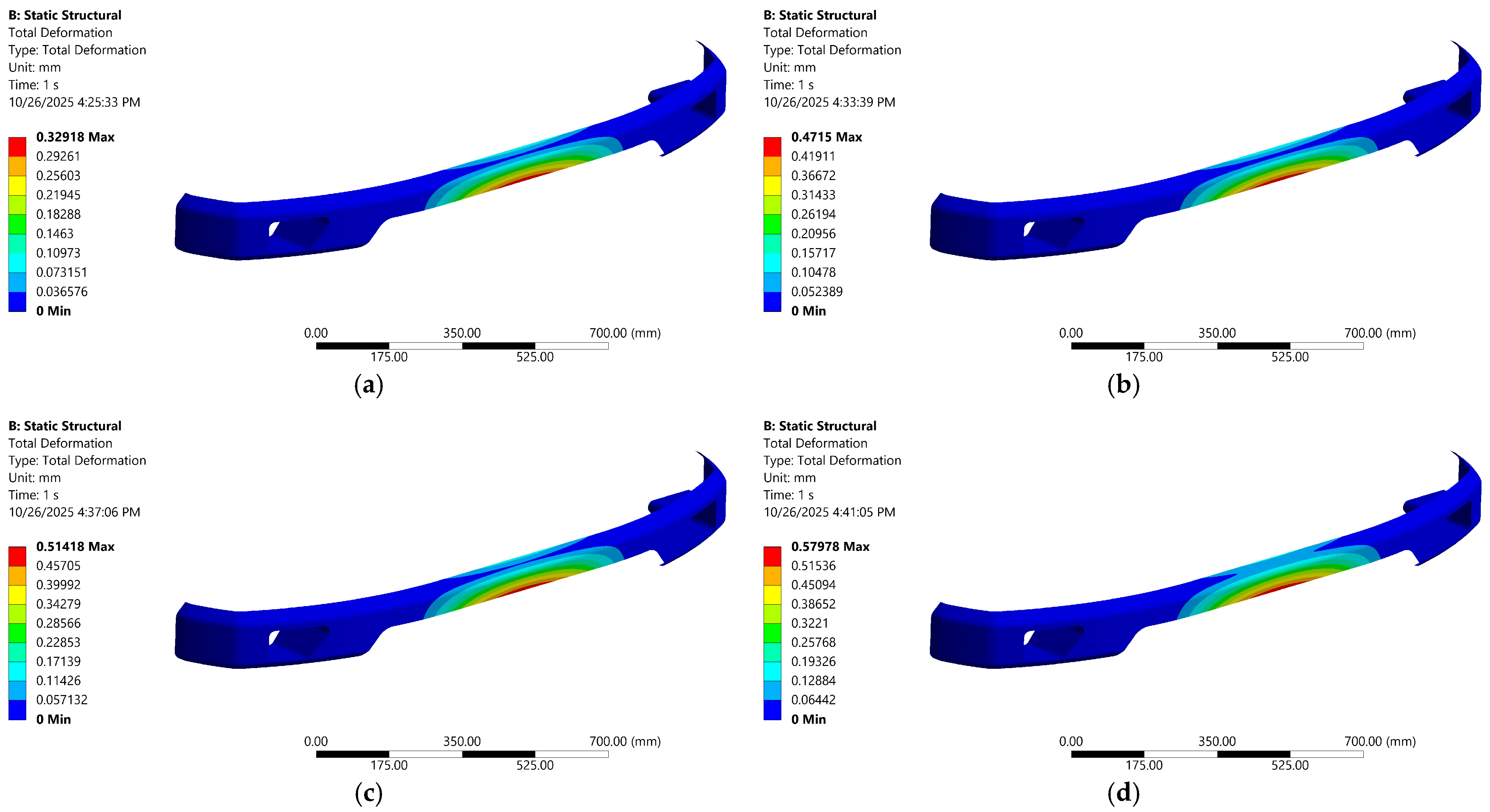
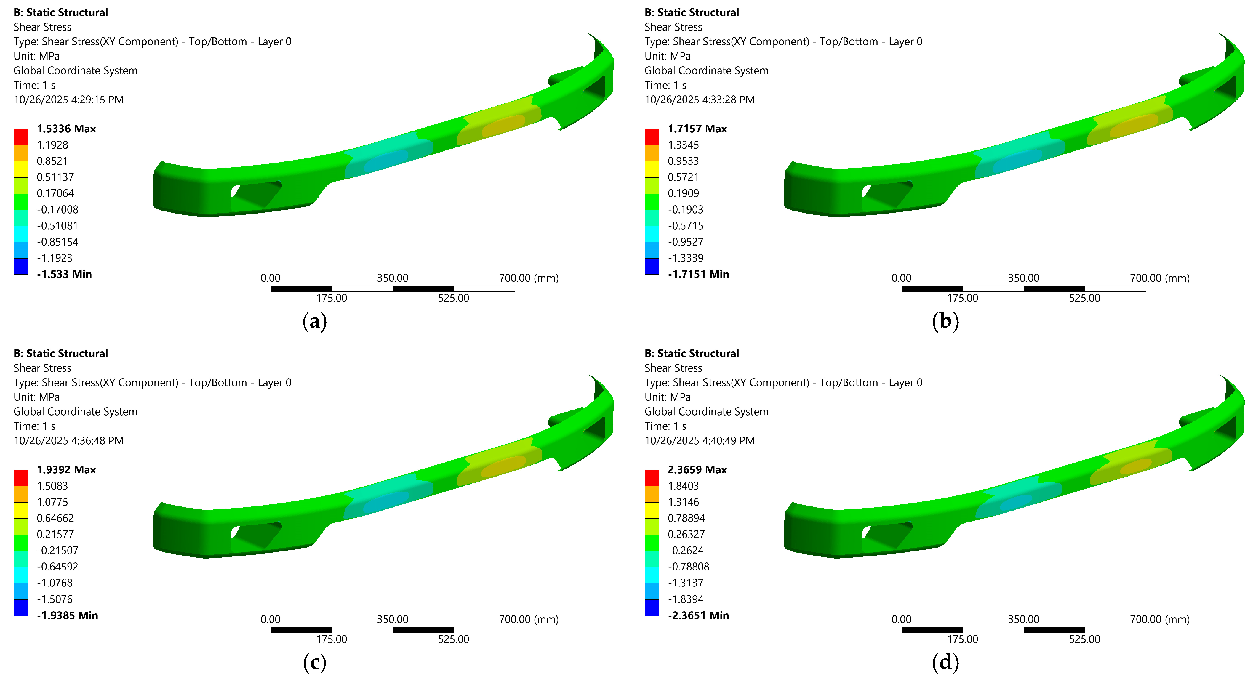
The 100% carbon–epoxy laminate deforms the most because it has the lowest effective stiffness, so under the same external load, it develops larger global and through-thickness strains. However, its shear stress is the weakest because the stack is materially homogeneous, where there are no stiffness mismatches between plies to create interlaminar stress concentrations, and because shear-stress scales with the shear modulus (τ = G·γ). In a compliant laminate, γ (shear strain) increases, but the much smaller G of carbon–epoxy limits τ, and the uniformity of properties spreads the load more evenly across the thickness. The net effect is high deformation but low peak shear stress, in contrast to hybrid layups where the modulus contrast follows a linear trend between interfacial shear and average deformation, as shown in the distribution contour (see Figure 14 and Figure 15).

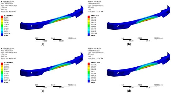
Figure 14. Distribution of total deformation in hybrid bumper material across different volume fractions of carbon–epoxy laminates; (a) 33.3%, (b) 50%, (c) 66.7%, (d) 83.3%.

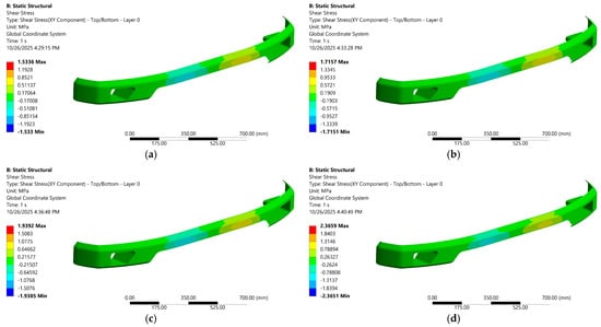
Figure 15. Shear-stress distribution in hybrid bumper material across different volume fractions of carbon–epoxy laminates; (a) 33.3%, (b) 50%, (c) 66.7%, (d) 83.3%.

Deformation trends indicate that replacing some positions in the carbon–epoxy laminate with CFRP layers progressively increases the laminate’s effective flexural modulus, resulting in lower deflections and shear stress under the same load. On the other hand, the shear behavior of carbon–epoxy laminates indicates interlayer interactions, which at a blend between 16.7 and 83.3%, strengthen interlaminar shear transfer with CFRP. Once the stack is fully carbon–epoxy (100%), the laminate becomes more homogeneous in thickness. These results demonstrate a trade-off: a lower carbon–epoxy fraction minimizes deformation and reduces shear-stress points. In contrast, a fully carbon–epoxy configuration offers the lowest shear concentration at the expense of the highest deformation. Ultimately, based on our findings, we elect to further investigate the combination of carbon–epoxy and CFRP reinforcement at a 50% volume fraction, where deformation and stress are balanced. Furthermore, it is clarified by Sharma et al. [62], who incorporated unidirectional carbon fiber in an epoxy with CFRP laminates. Moreover, Kaplan et al. [63] reported that the CFRP surface is compatible with epoxy resin, thereby increasing joint strength in hybrid joints.

3.4. Advanced Dynamic Analysis

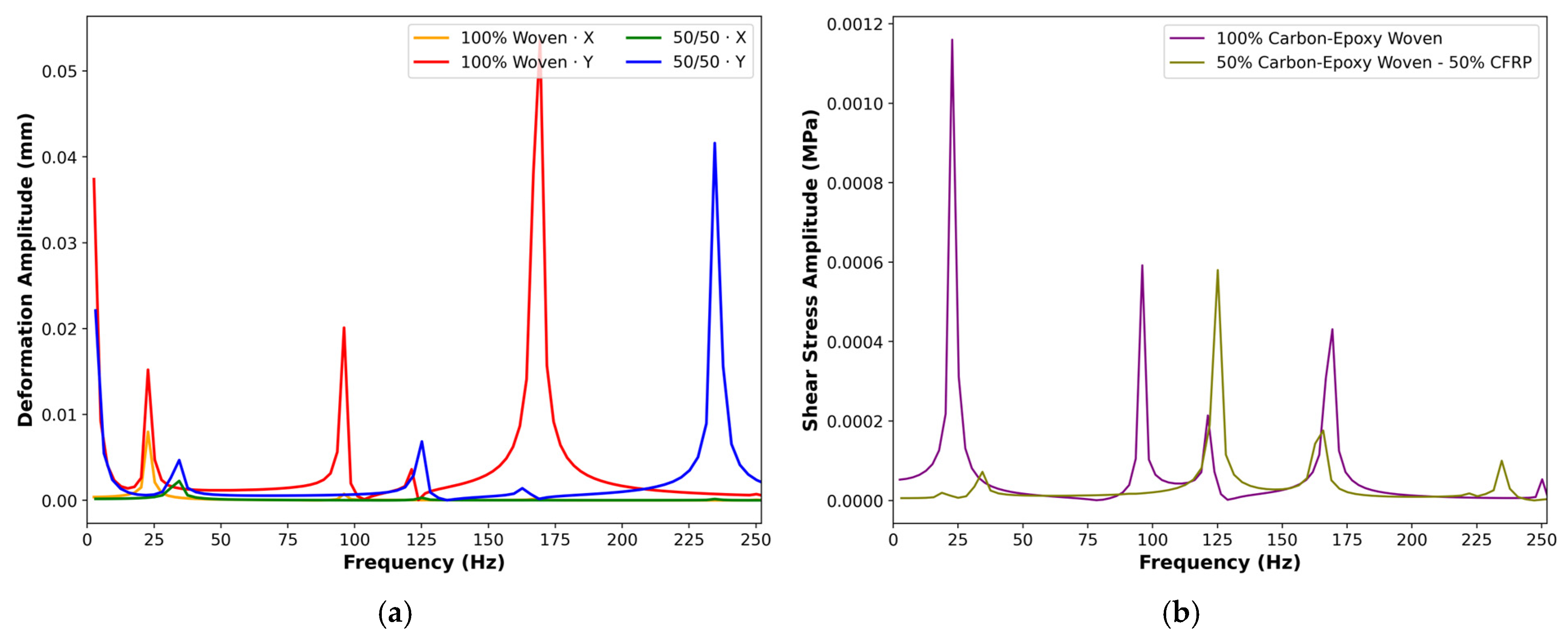
Extending the static analyses, we examined the frequency-domain (transient) response to understand how small operational vibrations could excite structural resonances. Using the same geometry, layups, and material properties, we applied a linear sweep. We recorded amplitudes of total deformation in the in-plane X and Y directions, and shear-stress amplitudes in the XY direction. Two architectures were compared on 100% woven carbon–epoxy and a 50/50 woven carbon–epoxy–CFRP hybrid.

The deformation spectra show (see Figure 16a) distinct resonant bands: a low-frequency peak, a mid-band resonance, and a high-frequency peak. The 100% woven laminate exhibits sharper and larger amplification, particularly in the Y direction, where one dominant mid-to-high-frequency mode surges well above the others. The 50/50 hybrid retains the same modal family but reduces peak amplitudes and subtly shifts/ broadens the resonances, indicating greater damping/energy spreading and a slightly stiffer effective response along one axis. Directional differences between X and Y further underscore the role of in-plane anisotropy in setting mode shapes and amplification.

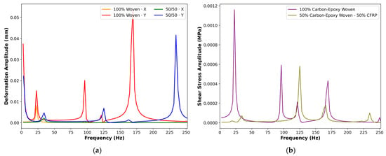
Figure 16. Response harmonic across different targets; (a) total deformation, (b) shear stress.

Meanwhile, shear-stress harmonics (see Figure 16b) mirror these trends. The entirely woven laminate shows higher stress amplitudes at each resonance, whereas the hybrid consistently suppresses peak shear and narrows stress hot spots. Together with the static findings, the harmonic results suggest that while woven layups aligned with load can control static deflection, hybridization with CFRP provides superior vibration robustness, lowering dynamic amplification and associated shear demands.

3.5. Frontal Impact Test Through Explicit Dynamics Analysis

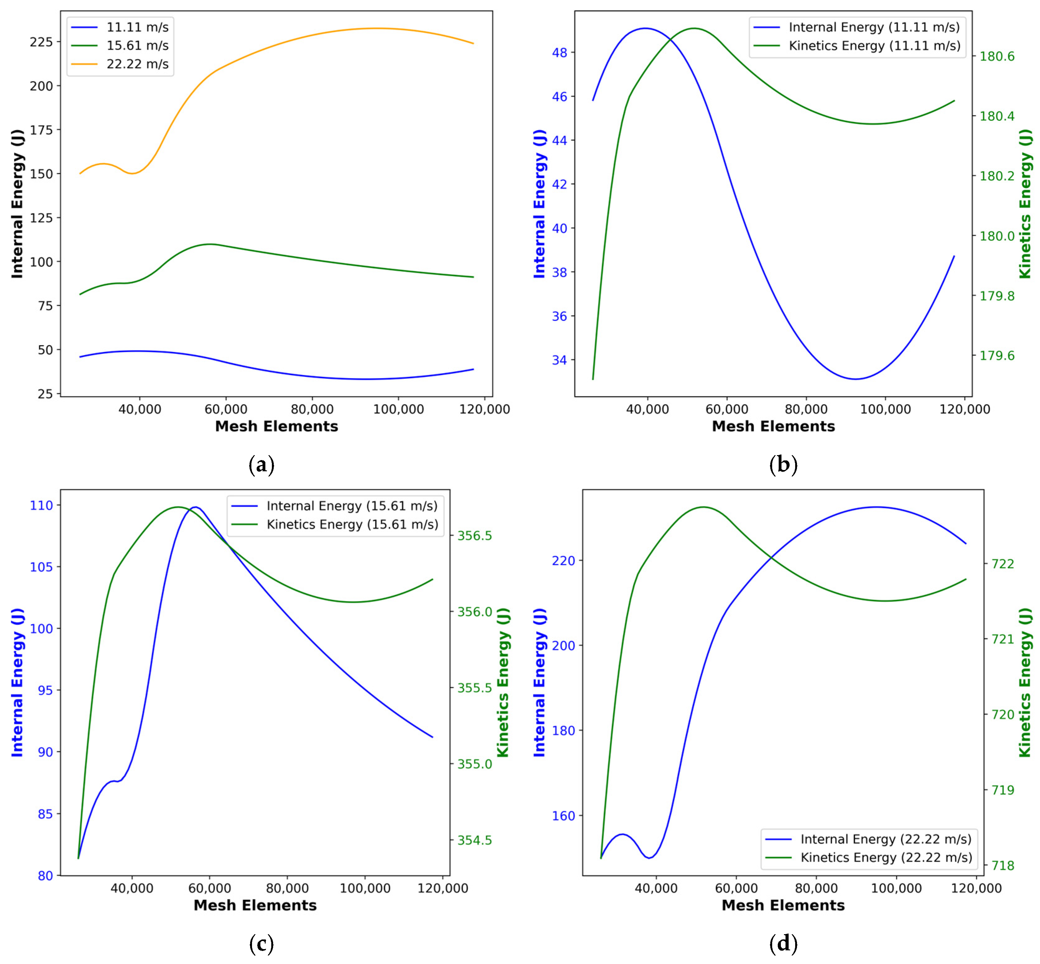
Bridging from 50% fractional volume levels in 6 mm thickness on a hybrid-composite of carbon–epoxy woven and CFRP as critical baselines, we now extend our investigation to dynamic loading by subjecting these hybrid laminates to frontal impact simulations via explicit dynamics at three distinct speeds, 11.11 m/s, 15.61 m/s, and 22.22 m/s. To identify an optimal discretization, we evaluated element sizes ranging from 6 mm to 11 mm, achieving convergence errors of 3–5% while avoiding excessive computational time. This setup captures stress-wave propagation and energy absorption (both internal and kinetic), revealing how the hybrid composite governs impact resistance and failure progression. For a detailed view of the resulting energy characteristics, see Figure 17.

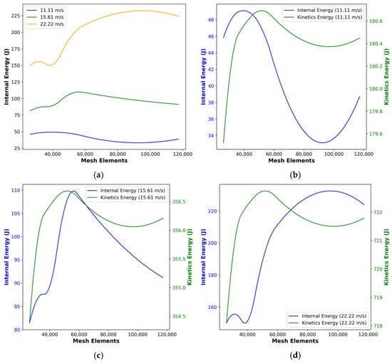
Figure 17. Energy absorption of bumper impact test; (a) internal energy in each speed test, and internal vs. kinetic energy correspond to mesh convergence in every speed test, (b) 11.11 m/s, (c) 15.61 m/s, (d) 22.22 m/s.

Figure 17a presents the mesh-refinement study of internal energy for frontal impact simulations at 11.11 m/s, 15.61 m/s, and 22.22 m/s. For all three speeds, the computed internal energy rises sharply as the mesh is refined from 25,000 to 55,000, then levels off or declines slightly beyond 80,000 elements. Specifically, the lowest speed (11.11 m/s) converges to 34–48 J of internal energy, while the mid-range speed (15.61 m/s) levels off near 80–110 J, and the highest speed (22.22 m/s) around 150–230 J. This non-monotonic behavior highlights an optimal mesh density (50,000 elements) that captures the bulk of damage and energy absorption without over-stiffening the response at extreme refinement.

Meanwhile, the next figures compare internal versus kinetic energy for each impact speed across the same mesh range. At 11.11 m/s (see Figure 17b), the internal energy peak (48 J) corresponds to a complementary dip in kinetic energy (180 J), after which both energies stabilize within ±0.5 J above 60,000 elements. The 15.61 m/s case (see Figure 17c) shows a broader internal energy maximum (110 J) and kinetic energy trough (356 J), indicating efficient conversion and dissipation at mid-mesh refinement. At 22.22 m/s (see Figure 17d), the energy exchange is most pronounced: internal energy climbs to 230 J as kinetic energy drops from 722 J, then both metrics reach a near-constant value past 70,000 elements. These convergence trends confirm that a mesh of 60,000–80,000 elements adequately resolve impact dynamics and energy partitioning for all tested speeds.

Based on the convergence trends by reviewing all in Figure 17, where internal and kinetic energies stabilize. Once it moves beyond roughly 60,000 elements, it is best to target a mesh of about 60,000. In practice, this corresponds to an element size of 7 mm. The intermediate-coarse element is enough to keep runtimes reasonable but fine enough to capture the bulk of stress-wave propagation and damage evolution with minimal error. For further visualization, bumper crash tests were performed via the explicit dynamics feature in Figure 18 as follows.

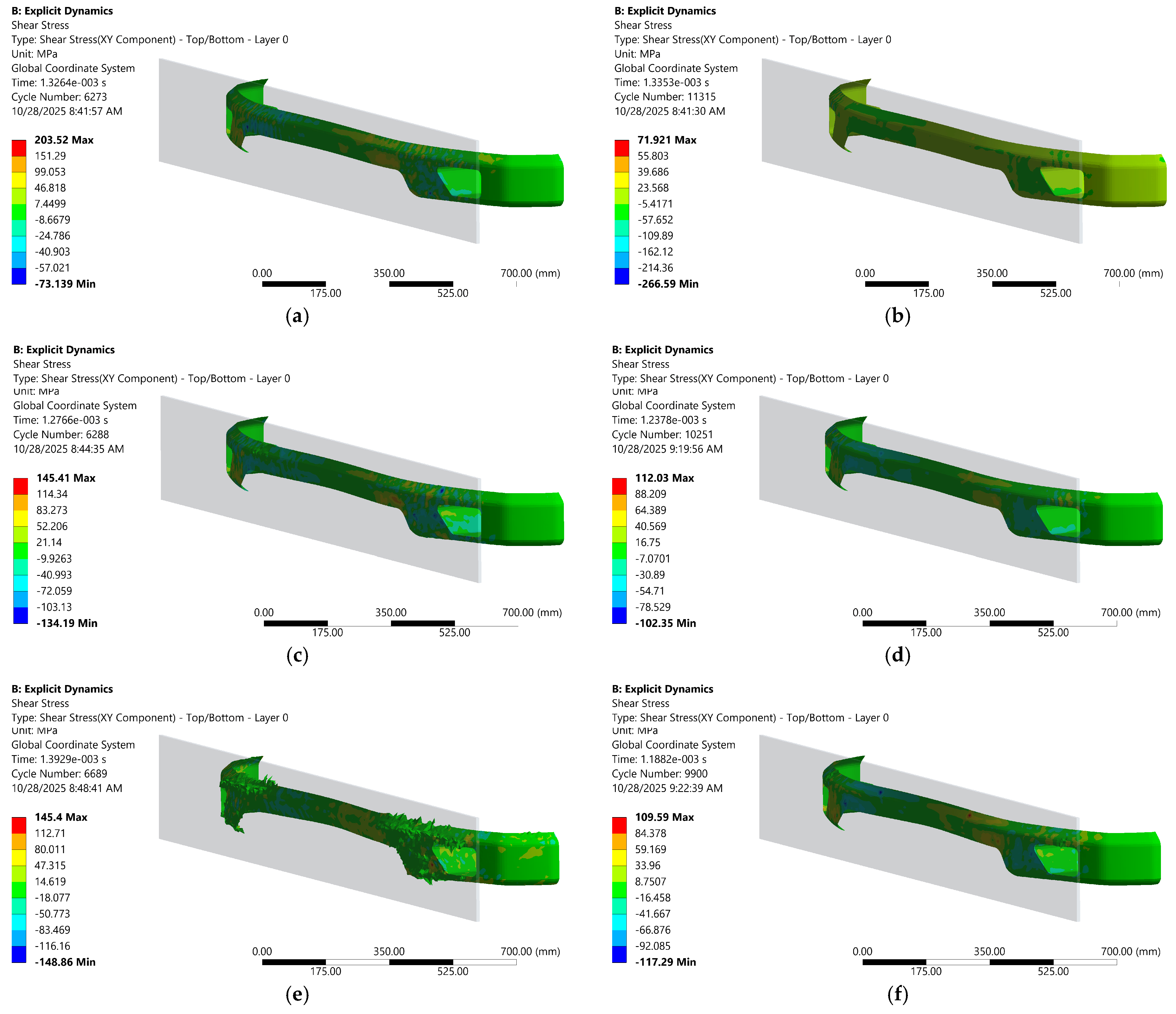
Figure 18. Shear-stress contour in frontal impact tests at various compositions and speeds; (a) 100% carbon–epoxy woven at 11.11 m/s, (b) 50% carbon–epoxy woven and 50% CFRP at 11.11 m/s, (c) 100% carbon–epoxy woven at 15.61 m/s, (d) 50% carbon–epoxy woven and 50% CFRP at 15.61 m/s, (e) 100% carbon–epoxy woven at 22.22 m/s, (f) 50% carbon–epoxy woven and 50% CFRP at 22.22 m/s.

As shown in Figure 18, there are contours which compare shear-stress distributions under frontal impact for fully woven carbon–epoxy and a 50/50 hybrid (carbon–epoxy woven + CFRP) across increasing velocities (11.11, 15.61, 22.22 m/s). In the 100% carbon–epoxy woven cases (see Figure 18a,c,e), rising speed produces widespread high-shear bands, coalescing into extended damage zones with visible crack initiation and propagation along the web and flange transitions, evidence of massive failure and shear localization that accelerates with impact energy. By contrast, the 50% carbon–epoxy woven and 50% CFRP laminate (see Figure 18b,d,f) maintains a more uniform, lower-amplitude shear field and retains its structural integrity even at the highest speed, with damage confined and less connected. Mechanistically, the hybrid’s higher stiffness and interfacial heterogeneity promote load redistribution, crack deflection/bridging, and greater energy dissipation, thereby suppressing catastrophic shear-driven crack growth seen in the homogeneous woven carbon–epoxy under comparable impact conditions.

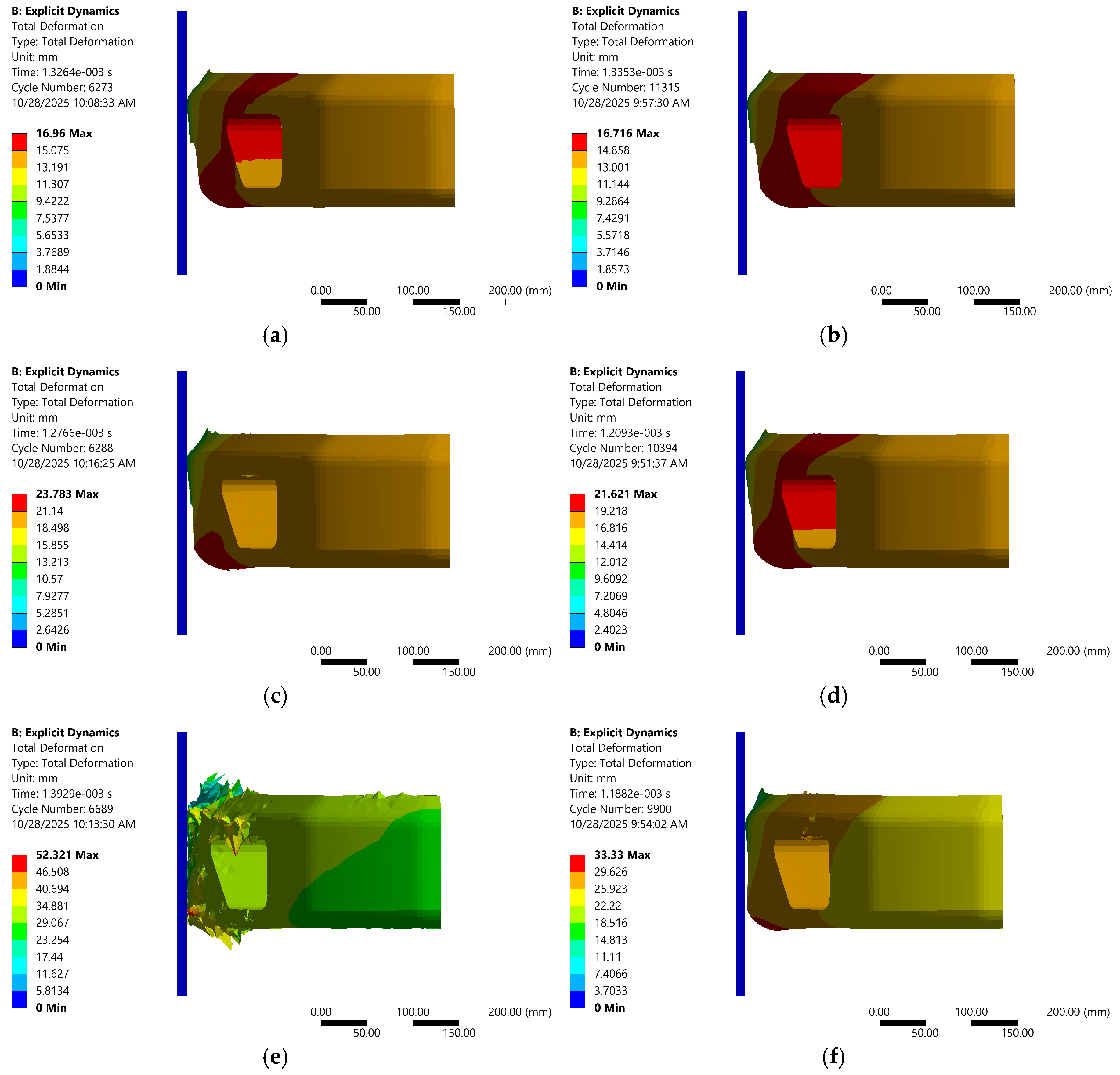
Consistent with the shear-stress fields in Figure 18, the total deformation maps in Figure 19 show a speed-dependent divergence in crash response between laminates. The 100% woven carbon–epoxy develops rapidly escalating global deflection with velocity, culminating at 22.22 m/s in extensive front-end collapse and unstable, nonrecoverable deformation consistent with shear-driven cracking and ply rupture. By contrast, the 50% woven carbon–epoxy/50% CFRP hybrid confines displacement to a smaller zone and preserves the primary load path even at the highest speed. This coupling of lower peak shear and lower average deformation in the hybrid implies more effective energy management.

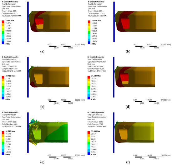
Figure 19. Total deformation contour in frontal impact tests at various compositions and speeds; (a) 100% carbon–epoxy woven at 11.11 m/s, (b) 50% carbon–epoxy woven and 50% CFRP at 11.11 m/s, (c) 100% carbon–epoxy woven at 15.61 m/s, (d) 50% carbon–epoxy woven and 50% CFRP at 15.61 m/s, (e) 100% carbon–epoxy woven at 22.22 m/s, (f) 50% carbon–epoxy woven and 50% CFRP at 22.22 m/s.

In addition, Figure 20 quantitatively consolidates these observations. The average total deformation increases with impact speed for both laminates. The 100% woven carbon–epoxy grows faster and remains higher at all speeds than the 50/50 hybrid, consistent with the broader collapse observed in Figure 18 and Figure 19. Maximum shear stress further explains the divergence: the entirely woven laminate shows extremely high shear stress at low speeds, which then drops as speed increases. In contrast, the hybrid stays much lower overall, reflecting more distributed load sharing and damage suppression. Thus, the summary plot confirms that hybridization simultaneously restrains deformation growth and caps shear peaks across the velocity range, aligning with the contour evidence of improved crashworthiness.

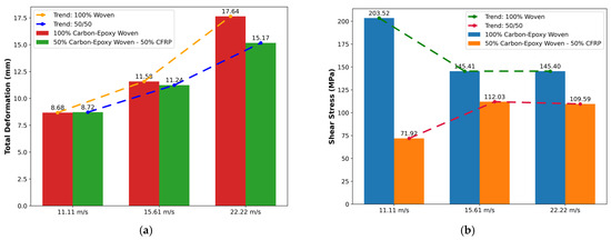
Figure 20. Bumper impact test plot; (a) total deformation (average), (b) shear stress (maximum).

3.6. Failure Mechanisms in Crash Events Based on Tsai–Wu Criterion

Extending the deformation–stress evidence (Figure 18, Figure 19 and Figure 20), we evaluated ply level failure using the Tsai–Wu criterion. In our post-processing, we report the inverse reserve factor (IRF = 1/RF) for each element; values approaching or exceeding 1 indicate that the Tsai–Wu failure index has been met, whereas lower values indicate remaining margin. The contour in Figure 21 highlights incipient failure bands aligned with the woven axes, with local IRF peaks at geometric discontinuities. These hotspots co-locate with the shear-stress concentrations and large deformation zones identified earlier, confirming that combined in-plane shear and bending drive the laminate toward its multiaxial strength envelope during crash loading.

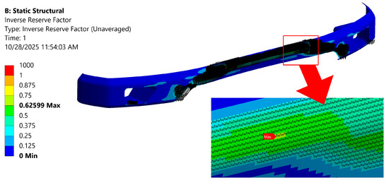
Figure 21. Failure mechanism of pure carbon–epoxy composites at the maximum point.

For the 100% woven carbon–epoxy, as impact speed increases, damage concentrates and pushes the IRF locally to unity, indicating fiber-dominated failure on the tensile face and matrix/shear failure in the compressive and web regions. The woven architecture provides bidirectional stiffness, but in a homogeneous stack, the lack of interfacial impedance changes allows cracks to nucleate and coalesce along weave tows and resin-rich paths, promoting delamination growth once the Tsai–Wu surface is reached. This agrees with the massive cracking and unstable collapse observed in the contour plots. Once local IRF 1 is achieved, stiffness degrades rapidly and deformation accelerates, producing the damage-driven softening trend captured by the shear-stress maxima.

3.7. Validation of Numerical Simulation via Machine Learning

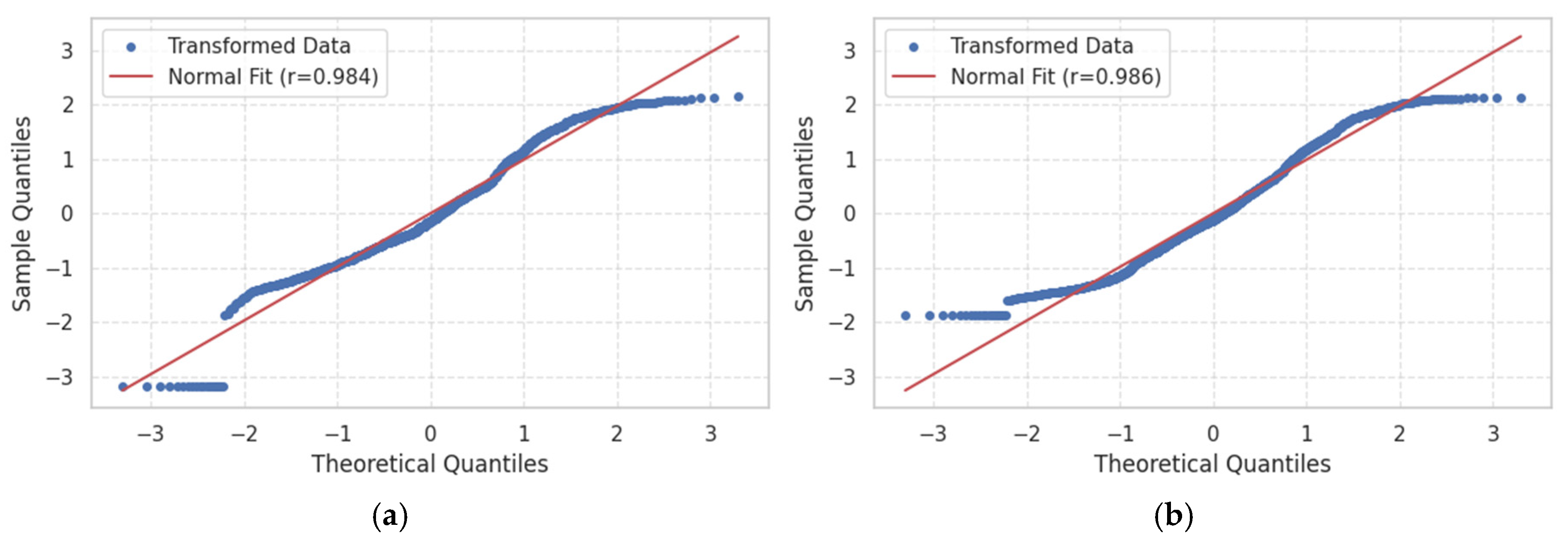
Building on previous results, this section employs a machine learning framework to quantitatively assess and refine the fidelity of our finite-element impact simulations. By training, supervised algorithms on a curated dataset of simulation outputs encompassing two targets by observing data normality in 11 features. We aim to cover correlations, identify predictive model parameters, and validate the normality of numerical simulation. The Q-Q plots below indicate the normality of the data by showing the distribution of the targets.

Figure 22 presents Q–Q plots of the transformed target variables against a theoretical normal distribution. In both plots, the blue dots closely follow the red reference line across the central range of quantiles, with only minor deviations in the tails, indicating that the transformed data are well approximated by normality. The Pearson correlation coefficients of 0.984 (see Figure 22a) for stress and 0.986 (see Figure 22b) for deformation further confirm that the transformations have effectively normalized the distributions, justifying the use of parametric techniques in subsequent machine learning validation.

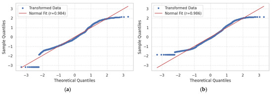
Figure 22. Q-Q plots of target; (a) shear stress, (b) total deformation.

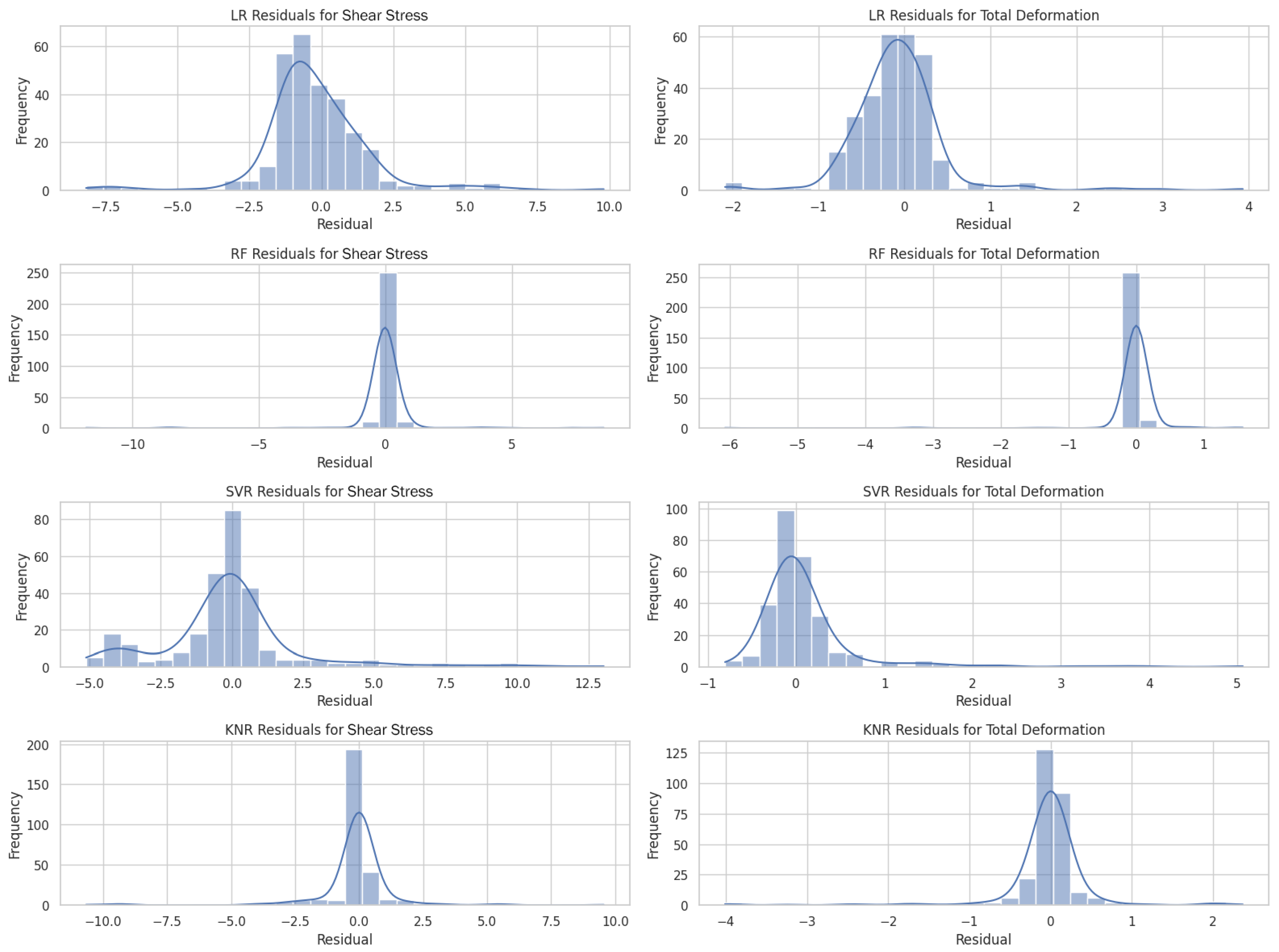
The residual analysis histograms (see Figure 23) reveal that, across all four regression algorithms, predictions of total deformation exhibit markedly tighter error distributions than those for shear stress. In particular, the Random Forest (RF) and k-nearest neighbors (KNN) models concentrate nearly all residuals within ±1 unit for both responses, especially for total deformation, where RF residuals are almost exclusively within ±0.5, indicative of minimal bias and low variance. In contrast, linear regression (LR) yields broader, heavy-tailed residuals (up to ±8 for stress and ±3.5 for deformation), betraying systematic under- and over-predictions at the extremes, while support vector regression (SVR) shows moderate skew and a few large positive stress residuals.

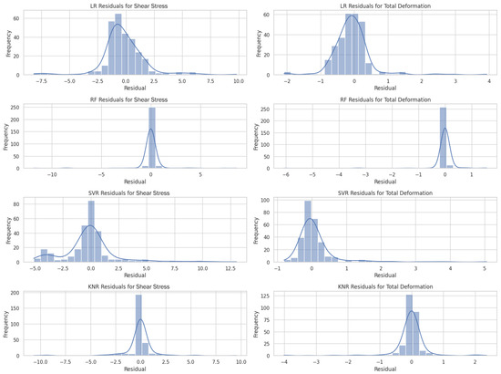
Figure 23. Residual histogram plot of targets based on model performance before calibration.

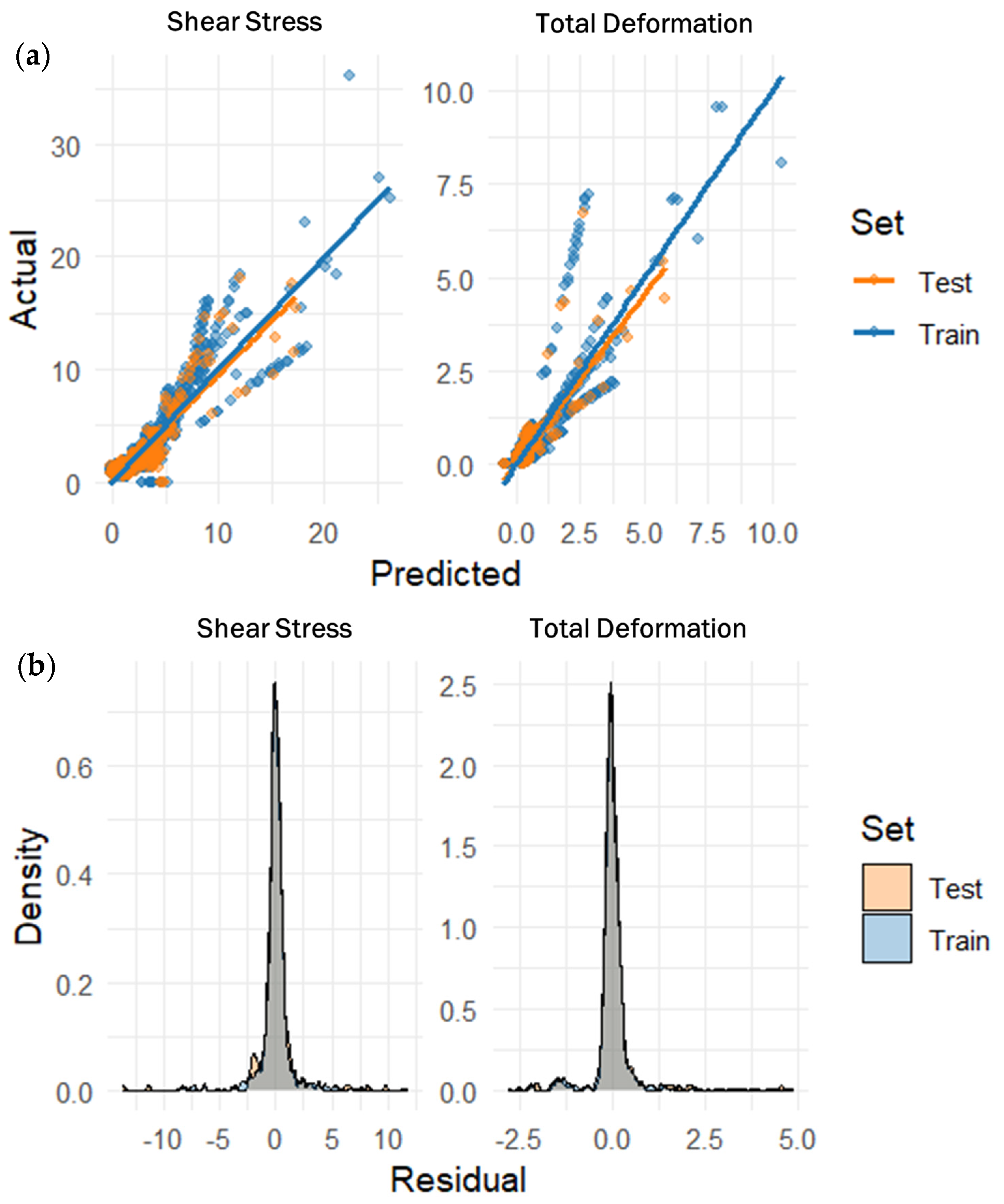
Consistent with the residual patterns before calibration in Figure 23, the Random Forest (RF) model (see Figure 24) is well calibrated for both targets: the train and test points cluster tightly around the 1:1 line in the predicted–actual plots, with only a few high-stress outliers indicating localized underestimation at the extreme tail. Post-calibration residual densities are sharply centered at zero and nearly symmetric, especially for total deformation, indicating minimal bias and low variance; shear stress shows a broader but narrower mode, reflecting inherently higher response variability rather than model misfit. The close overlap of the train and test curves indicates good generalization with limited overfitting. At the same time, the thin, homoscedastic residual spread across the prediction range supports the RF’s robustness as a downstream surrogate for interrogating design trade-offs and uncertainty in impact simulations.

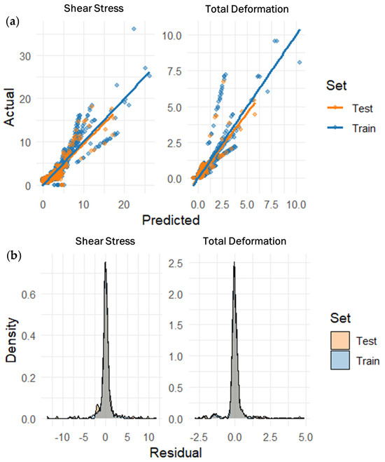
Figure 24. Train and test validation of Random Forest (RF); (a) calibration curve, (b) residual density after calibration.

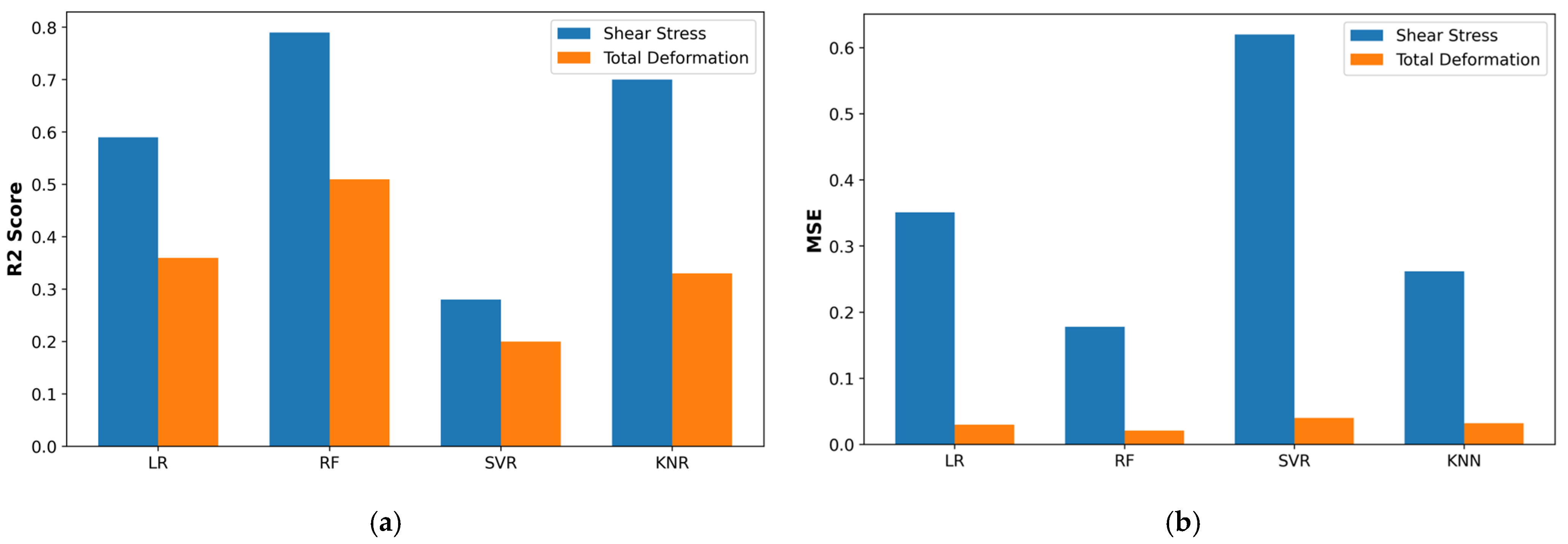
Further visualizations of the shear-stress predictions are presented for the train and test sets across several models (see Figure 25). Random Forest (RF) regressor clearly outperforms the other algorithms: it achieves the lowest mean squared error (0.18) and the highest R² (0.79), indicating both high accuracy and strong variance explanation on unseen data. Linear regression (LR) comes next, with moderate error (MSE of 0.35) and an R² of 0.59, suggesting a reasonable but ultimately limited linear fit. Support vector regression (SVR) performs worst on stress, with an MSE exceeding 0.6 and an R² below 0.30, suggesting underfitting or sensitivity to outliers. K-nearest neighbors (KNN) lies between LR and RF, delivering lower error than LR (MSE = 0.26) and a solid R² of 0.70, but still falling short of RF’s ensemble-learning advantage.

Figure 25. Model performance evaluation; (a) R² Score, (b) MSE (mean squared error).

For total deformation predictions, a similar hierarchy emerges: RF again yields the best results (MSE = 0.23, R² = 0.51), confirming its robustness across both targets. SVR remains the weakest for deformation (MSE = 0.38, R² = 0.20), reinforcing that its kernel-based approach may struggle with this dataset’s complexity. Linear regression and KNN perform comparably in the mid-range: LR gives an MSE of 0.30 with R² at 0.37, while KNN slightly improves on error (MSE at 0.33) but with a similar R² of 0.33. These findings demonstrate that the RF model generalizes most effectively to new simulation data, whereas SVR is the least reliable for both stress and deformation predictions. Overall, RF outperforms all models in terms of compactness and residual symmetry, indicating superior generalization and robustness when modeling shear stress and total deformation on our finite-element dataset.

The Random Forest (RF) algorithm demonstrated clear advantages over linear regression (LR), support vector regression (SVR), and K-nearest neighbors (KNN), due to its ability to capture nonlinear, multivariate relationships among structural parameters such as ply number, mesh density, fiber angle, and applied load. Unlike LR, which assumes linear dependence, RF constructs an ensemble of decorrelated decision trees, allowing it to approximate complex stress–strain interactions arising from anisotropic composite behavior. Moreover, the bootstrap aggregation (bagging) technique inherent to RF minimizes overfitting and enhances prediction stability, even when the dataset contains numerical noise or missing values. Compared with SVR, which exhibited kernel sensitivity and residual skewness, and KNN, which tends to perform poorly in high-dimensional spaces, RF produced consistently low residuals (±0.5) and symmetric error distributions. Feature-importance analysis further showed that ply count, mesh convergence, and load magnitude contributed most to predictive accuracy, aligning closely with the physical mechanisms influencing shear stress and deformation.

Based on previous research, several studies have also identified Random Forest as one of the most accurate and reliable algorithms for predicting mechanical or structural behaviors of composite and cement-based materials. For instance, research by Tao and Xue [64] reported that a PSO-RF hybrid model achieved a high prediction accuracy (R² = 0.963) in forecasting FRP-to-concrete bond strength, outperforming other regression methods. Similarly, Zhang et al. [65] demonstrated that RF produced highly accurate predictions of compressive strength in green cement-based composites under thermal stress. Joo et al. [66] and Huang and Adityawardhana [67] also highlighted that RF exhibited robust generalization and interpretability through feature-importance analysis in polymer and metal-matrix composites, respectively. These findings collectively reinforce that RF’s ensemble architecture provides superior performance, robustness, and physical interpretability, which is consistent with the outcomes of this study.

In summary, the current results and evidence from prior studies consistently confirm that Random Forest delivers the highest accuracy and reliability among the tested models for predicting shear stress and total deformation in composite structures. Its ensemble-based learning mechanism, resistance to overfitting, and ability to link statistical predictions with physical interpretability establish RF as the most effective and trustworthy data-driven approach for modeling composite bumpers.

4. Conclusions

In this study, we successfully integrated finite element simulation, controlled impact tests, and multivariate machine learning to optimize the design of a multi-layered automobile bumper using the Tsai–Wu criterion as the primary failure model. However, numerical analysis highlighted limitations in distinguishing between failure modes and their interaction coefficients experimentally. To address this issue, we employ ANSYS software with a Fortran program, which enables more accurate estimation of failure behavior, resulting in an average error of 13.19%. Based on our observations, the 2 mm mesh size of the 50%/50% woven carbon–epoxy/CFRP laminate (hybrid composite) at 6 mm thickness in 0° orientation showed the best uniformity in shear stress, and the observed deformation converged towards a stable value, which validated the suitability of this configuration for further analysis. Furthermore, the combination of carbon–epoxy with CFRP can be a promising hybrid material, as indicated by our main findings. To capture coupled mechanical behavior, total deformation was incorporated alongside shear stress as a secondary target in our ML framework. Across a suite of regression algorithms, the Random Forest (RF) model emerged as the most reliable predictor. These findings demonstrate a rapid pathway for data-driven design and a path for broader applications of ML-enhanced multivariate analyses in engineering.

References

- Nations, U. Road Traffic Injuries. Available online: https://www.who.int/news-room/fact-sheets/detail/road-traffic-injuries (accessed on 29 October 2025).
- Chang, F.R.; Huang, H.L.; Schwebel, D.C.; Chan, A.H.S.; Hu, G.Q. Global road traffic injury statistics: Challenges, mechanisms and solutions. Chin. J. Traumatol. 2020, 23, 216–218. [Google Scholar] [CrossRef]
- Conceição, P.; Calderón, C.; Gautam, P.; Ghorai, M.; Goyal, D.; Hsu, Y.-C.; Lengfelder, C.; Lutz, B.; Mirza, T.; Mohammed, R.; et al. Human Development Report 2023/2024. New York: United Nation Development Programme. 2024. Available online: https://hdr.undp.org/system/files/documents/global-report-document/hdr2023-24reporten.pdf (accessed on 29 October 2025).
- Adom, P.K. The socioeconomic impact of climate change in developing countries over the next decades: A literature survey. Heliyon 2024, 10, e35134. [Google Scholar] [CrossRef]
- World Health Organization. Decade of Action for Road Safety 2021–2030. Available online: https://www.who.int/teams/social-determinants-of-health/safety-and-mobility/decade-of-action-for-road-safety-2021-2030 (accessed on 29 October 2025).
- Jan, D.; Khan, M.S.; Ud Din, I.; Khan, K.A.; Shah, S.A.; Jan, A. A review of design, materials, and manufacturing techniques in bumper beam system. Compos. Part C Open Access 2024, 14, 100496. [Google Scholar] [CrossRef]
- Khan, F.; Hossain, N.; Mim, J.J.; Rahman, S.M.; Iqbal, M.J.; Billah, M.; Chowdhury, M.A. Advances of composite materials in automobile applications—A review. J. Eng. Res. 2025, 13, 1001–1023. [Google Scholar] [CrossRef]
- Kılıç, E.; Fullana-i-Palmer, P.; Fullana, M.; Delgado-Aguilar, M.; Puig, R. Circularity of new composites from recycled high density polyethylene and leather waste for automotive bumpers. Testing performance and environmental impact. Sci. Total Environ. 2024, 919, 170413. [Google Scholar] [CrossRef]
- Tsirogiannis, E.C.; Daskalakis, E.; Vogiatzis, C.; Psarommatis, F.; Bartolo, P. Advanced composite armor protection systems for military vehicles: Design methodology, ballistic testing, and comparison. Compos. Sci. Technol. 2024, 251, 110486. [Google Scholar] [CrossRef]
- Isaac, G.; Adams, J.; Dr, S.; Lie, S. Design for the Environmental Emergency: Plastic Chairs and the Transition to Low-Carbon Product Design. 2022. Available online: https://hdl.handle.net/10453/161828 (accessed on 30 October 2025).
- Andrady, A.L.; Heikkilä, A.M.; Pandey, K.K.; Bruckman, L.S.; White, C.C.; Zhu, M.; Zhu, L. Effects of UV radiation on natural and synthetic materials. Photochem. Photobiol. Sci. 2023, 22, 1177–1202. [Google Scholar] [CrossRef]
- Bandaru, A.K.; Chouhan, H.; Ma, H.; Kothandan, D.K.; O’Higgins, R.M. Ballistic impact response of Elium® thermoplastic composites reinforced with high-performance fibres in monolithic and hybrid configurations. Compos. B Eng. 2026, 309, 113030. [Google Scholar] [CrossRef]
- Sharma, H.; Kumar, A.; Rana, S.; Sahoo, N.G.; Jamil, M.; Kumar, R.; Sharma, S.; Li, C.; Kumar, A.; Eldin, S.M.; et al. Critical review on advancements on the fiber-reinforced composites: Role of fiber/matrix modification on the performance of the fibrous composites. J. Mater. Res. Technol. 2023, 26, 2975–3002. [Google Scholar] [CrossRef]
- Khoshmardan, M.A.; Behbahani, T.J.; Ghotbi, C.; Hassanpouryouzband, A.; Nasiri, A. Experimental study of polymeric composite reinforced with carbon fiber for mud lost control application. Sci. Rep. 2024, 14, 25225. [Google Scholar] [CrossRef]
- Bahubalendruni, M.V.A.R.; Parhi, D.; Jena, P.C.; Raghavendra, G.; Mohamed, A.; Rajan, B.G.; Padmanabhan, S.; Gautam, D.; Khan, F.; Baskar, S.; et al. An Investigation into the Design and Analysis of the Front Frame Bumper with Dynamic Load Impact. Eng. Proc. 2024, 66, 6. [Google Scholar] [CrossRef]
- Yeshanew, E.S.; Ahmed, G.M.S.; Sinha, D.K.; Badruddin, I.A.; Kamangar, S.; Alarifi, I.M.; Hadidi, H.M. Experimental investigation and crashworthiness analysis of 3D printed carbon PA automobile bumper to improve energy absorption by using LS-DYNA. Adv. Mech. Eng. 2023, 15, 16878132231181058. [Google Scholar] [CrossRef]
- Ul Abrar, M.S.; Nadim Ezaz, K.F.; Hasan, M.J.; Pranto, R.I.; Alvy, T.A.; Hossain, M.Z. Speed-dependent impact analysis on a car bumper structure using various materials. Results Eng. 2024, 21, 101927. [Google Scholar] [CrossRef]
- Cui, J.; Hao, H.; Shi, Y. Discussion on the suitability of concrete constitutive models for high-rate response predictions of RC structures. Int. J. Impact Eng. 2017, 106, 202–216. [Google Scholar] [CrossRef]
- Koochi, A.; Abadyan, M. Differential equations in miniature structures. In Nonlinear Differential Equations in Micro/Nano Mechanics; Elsevier: Amsterdam, The Netherlands, 2020; pp. 1–30. [Google Scholar] [CrossRef]
- Chen, X.; Sun, X.; Chen, P.; Wang, B.; Gu, J.; Wang, W.; Chai, Y.; Zhao, Y. Rationalized improvement of Tsai–Wu failure criterion considering different failure modes of composite materials. Compos. Struct. 2021, 256, 113120. [Google Scholar] [CrossRef]
- Rahimi, N.; Musa, M.; Hussain, A.K.; Mahmud, J. Finite element implementations to predict the failure of composite laminates under uniaxial tension. Adv. Mat. Res. 2012, 499, 20–24. [Google Scholar] [CrossRef]
- Joo, S.J.; Yu, M.H.; Seock Kim, W.; Lee, J.W.; Kim, H.S. Design and manufacture of automotive composite front bumper assemble component considering interfacial bond characteristics between over-molded chopped glass fiber polypropylene and continuous glass fiber polypropylene composite. Compos. Struct. 2020, 236, 111849. [Google Scholar] [CrossRef]
- Dhamone, S.P.; Padmakumar, A. Analysis of a Crash on a Vehicle System by Adjusting Appropriate Input Parameters to Manage Energy Absorption Capacity for Enhancing Passenger Safety. Acta Innov. 2023, 2023, 5–17. [Google Scholar] [CrossRef]
- Nawawithan, N.; Kittisakpairach, P.; Nithiboonyapun, S.; Ruangjirakit, K.; Jongpradist, P. Design and performance simulation of hybrid hemp/glass fiber composites for automotive front bumper beams. Compos. Struct. 2024, 335, 118003. [Google Scholar] [CrossRef]
- Yeshanew, E.S.; Nallamothu, R.B. Numerical Simulation and Design Modification of an Automotive Bumper to Enhance Energy Absorption by Using LS-DYNA. Model. Simul. Eng. 2025, 2025, 9980385. [Google Scholar] [CrossRef]
- Li, G.; Lyons, M.; Wang, B.; Yang, J.; Otte, D.; Simms, C. The influence of passenger car front shape on pedestrian injury risk observed from German in-depth accident data. Accid. Anal. Prev. 2017, 101, 11–21. [Google Scholar] [CrossRef]
- Lotfy, M.N.; Khalifa, Y.A.; Dessouki, A.K.; Fathallah, E. Dynamic Behavior of Steel and Composite Ferry Subjected to Transverse Eccentric Moving Load Using Finite Element Analysis. Appl. Sci. 2020, 10, 5367. [Google Scholar] [CrossRef]
- Mahmoud, A.M. Strengthening of concrete beams having shear zone openings using orthotropic CFRP modeling. Ain Shams Eng. J. 2012, 3, 177–190. [Google Scholar] [CrossRef]
- Widyianto, A.; Budiman, Y.; Anugrah, R.A.; Fatin, N.N.; Sutopo Wibowo, H. Optimizing enhanced smart architecture frame (eSAF) topology: A computational approach to weight and strength trade-offs. Results Eng. 2025, 28, 107614. [Google Scholar] [CrossRef]
- Ren, S.; Zhang, P.; Wu, Q.; Zhang, Q.; Gong, Z.; Song, G.; Long, R.; Gong, L.; Wu, M. Review of bumper materials for spacecraft shield against orbital debris hypervelocity impact. Def. Technol. 2025, 45, 137–177. [Google Scholar] [CrossRef]
- Bergström, J. Elasticity/Hyperelasticity. In Mechanics of Solid Polymers; William Andrew: Norwich, NY, USA, 2015; pp. 209–307. [Google Scholar] [CrossRef]
- Ghadimi, B.; Nikraz, H. A comparison of implementation of linear and nonlinear constitutive models in numerical analysis of layered flexible pavement. Road Mater. Pavement Des. 2017, 18, 550–572. [Google Scholar] [CrossRef]
- Vlach, J.; Doubrava, R.; Růžek, R.; Raška, J.; Horňas, J.; Kadlec, M. Linearization of Composite Material Damage Model Results and Its Impact on the Subsequent Stress–Strain Analysis. Polymers 2022, 14, 1123. [Google Scholar] [CrossRef]
- Menga, E.; Hernandez, S.; Moledo, S.; Lopez, C. Nonlinear dynamic analysis of assembled aircraft structures with concentrated nonlinearities. In Proceedings of the International Forum on Aeroelasticity and Structural Dynamics, Saint Petersburg, Russia, 28 June–2 July 2015. [Google Scholar]
- Li, S.; Sitnikova, E.; Liang, Y.; Kaddour, A.-S. Rationalisation of the Tsai-Wu failure criterion. In Proceedings of the ICCM International Conferences on Composite Materials, Xi’an, China, 20–25 August 2017. [Google Scholar]
- Li, S.; Sitnikova, E.; Liang, Y.; Kaddour, A.S. The Tsai-Wu failure criterion rationalised in the context of UD composites. Compos. Part A Appl. Sci. Manuf. 2017, 102, 207–217. [Google Scholar] [CrossRef]
- Soni, S.R. A Comparative Study of Failure Envelopes in Composite Laminates. J. Reinf. Plast. Compos. 1983, 2, 34–42. [Google Scholar] [CrossRef]
- Huybrechts, S.; Maji, A.; Lao, J.; Wegner, P.; Meink, T. Validation of the quadratic composite failure criteria with out-of-plane shear terms. J. Compos. Mater. 2002, 36, 1879–1888. [Google Scholar] [CrossRef]
- Rahimi, N.; Rahim, M.A.; Hussain, A.K.; Mahmud, J. Evaluation of failure criteria for composite plates under tension. In Proceedings of the 2012 IEEE Symposium on Humanities, Science and Engineering Research, Kuala Lumpur, Malaysia, 24–27 June 2012; IEEE: New York City, NY, USA, 2012; pp. 849–854. [Google Scholar] [CrossRef]
- Tsai, S.W.; Wu, E.M. A General Theory of Strength for Anisotropic Materials. J. Compos. Mater. 1971, 5, 58–80. [Google Scholar] [CrossRef]
- Takács, D.M.; Berezvai, S.; Kovács, L. A general method for numerical identifiability and sensitivity analysis of failure criteria for continuous fibre-reinforced plastics. Eur. J. Mech.-A/Solids 2023, 100, 104976. [Google Scholar] [CrossRef]
- Khedkar, N.K.; Sonawane, C.R.; Kumar, S. Experimental and static numerical analysis on bumper beam to be proposed for Indian passenger car. Mater. Today Proc. 2021, 42, 383–387. [Google Scholar] [CrossRef]
- Zhao, H.; Xu, P.; Li, B.; Yao, S.; Yang, C.; Guo, W.; Xiao, X. Full-Scale Train-to-Train Impact Test and Multi-Body Dynamic Simulation Analysis. Machines 2021, 9, 297. [Google Scholar] [CrossRef]
- Mallikarjuna, A.; Marghitu, D.; Raju, P.K. Simulation of Dynamic Event of Impact Using Explicit 3D Fem Model and Validation by Experiment and Contact Models. Int. J. Eng. Appl. Sci. Technol. 2021, 6, 51–61. [Google Scholar] [CrossRef]
- Karthikeyan, M.; Jenarthanan, M.P.; Giridharan, R.; Shunmugesh, K. Investigation on Crash Analysis of a Frontal Car Bumper. Trans. Indian Inst. Met. 2019, 72, 2699–2709. [Google Scholar] [CrossRef]
- Idrees, U.; Ahmad, S.; Shah, I.A.; Talha, M.; Shehzad, R.; Amjad, M.; Rahiamin Koloor, S.S. Finite element analysis of car frame frontal crash using lightweight materials. J. Eng. Res. 2023, 11, 100007. [Google Scholar] [CrossRef]
- Patil, H.; Jeyakarthikeyan, P.V. Mesh convergence study and estimation of discretization error of hub in clutch disc with integration of ANSYS. In Proceedings of the IOP Conference Series: Materials Science and Engineering. Institute of Physics Publishing, Ekaterinburg, Russia, 26–29 August 2018. [Google Scholar]
- Alarifi, I.M. Simulation and Mechanical Testing of 3D Printing Shin Guard Composite Materials. Virtual. Phys. Prototyp. 2024, 19, 1–14. [Google Scholar] [CrossRef]
- Samuel, O.W.; Asogbon, G.M.; Sangaiah, A.K.; Li, G. Computational Intelligence Enabling the Development of Efficient Clinical Decision Support Systems: Case Study of Heart Failure. In Computational Intelligence for Multimedia Big Data on the Cloud with Engineering Applications; Academic Press: Cambridge, MA, USA, 2018; pp. 123–133. [Google Scholar] [CrossRef]
- Monsen, K.A. Intervention Effectiveness Research: Quality Improvement and Program Evaluation in Healthcare: A Practical Guide to Real-World Implementation; Springer: Berlin/Heidelberg, Germany, 2024; pp. 1–254. ISBN 9783031541117. [Google Scholar]
- Gunadi Widyianto, A.; Budiman, Y.; Wahyudi, K.S.; Adiyasa, I.W.; Fauzi, N.A.; Arifin, Z.; Tun, N.N. Comparison of Brake Cooling System on Bus: Simulation and Evaluation of Natural vs Forced Air through Machine Learning Processing. J. Adv. Res. Fluid Mech. Therm. Sci. 2025, 126, 178–200. [Google Scholar] [CrossRef]
- Xu, W.; Huang, S.H.; Su, J.; Gudi, S.; O’Sullivan, B. Statistical fundamentals on cancer research for clinicians: Working with your statisticians. Clin. Transl. Radiat. Oncol. 2021, 27, 75–84. [Google Scholar] [CrossRef]
- Chicco, D.; Warrens, M.J.; Jurman, G. The coefficient of determination R-squared is more informative than SMAPE, MAE, MAPE, MSE and RMSE in regression analysis evaluation. PeerJ Comput. Sci. 2021, 7, e623. [Google Scholar] [CrossRef]
- Amir, A.L.; Ishak, M.R.; Yidris, N.; Zuhri, M.Y.M.; Asyraf, M.R.M.; Zakaria, S.Z.S. Influence of Woven Glass-Fibre Prepreg Orientation on the Flexural Properties of a Sustainable Composite Honeycomb Sandwich Panel for Structural Applications. Materials 2023, 16, 5021. [Google Scholar] [CrossRef]
- Ho, D.H.; Choi, Y.Y.; Ki, S.Y.; Kim, D.H.; Cho, J.H. Getting in line: Filler alignment strategies for anisotropic composite fabrication. Compos. B Eng. 2025, 305, 112626. [Google Scholar] [CrossRef]
- Ricciardi, M.R.; Papa, I.; Lopresto, V.; Calzolari, A.; Vigna, L.; Antonucci, V. Experimental characterization of the crashworthiness of carbon fiber reinforced epoxy composites. Prog. Aerosp. Sci. 2024, 148, 101003. [Google Scholar] [CrossRef]
- Hao, W.; Ge, D.; Ma, Y.; Yao, X.; Shi, Y. Experimental investigation on deformation and strength of carbon/epoxy laminated curved beams. Polym. Test. 2012, 31, 520–526. [Google Scholar] [CrossRef]
- Liu, F.; Deng, S.; Zhang, J. Mechanical Properties of Epoxy and Its Carbon Fiber Composites Modified by Nanoparticles. J. Nanomater. 2017, 2017, 8146248. [Google Scholar] [CrossRef]
- Kim, M.T.; Rhee, K.Y.; Lee, J.H.; Hui, D.; Lau, A.K.T. Property enhancement of a carbon fiber/epoxy composite by using carbon nanotubes. Compos. B Eng. 2011, 42, 1257–1261. [Google Scholar] [CrossRef]
- Mohamed, Y.S.; Abdelbary, A. Theoretical and experimental study on the influence of fiber orientation on the tensile properties of unidirectional carbon fiber/epoxy composite. Alex. Eng. J. 2023, 67, 693–705. [Google Scholar] [CrossRef]
- Dutt, A. Effect of Mesh Size on Finite Element Analysis of Beam. Int. J. Mech. Eng. 2019, 2, 8–10. [Google Scholar] [CrossRef]
- Sharma, H.; Kumar, A.; Rana, S.; Guadagno, L. An Overview on Carbon Fiber-Reinforced Epoxy Composites: Effect of Graphene Oxide Incorporation on Composites Performance. Polymers 2022, 14, 1548. [Google Scholar] [CrossRef]
- Kaplan, N.; Gulluoglu, A.N.; Turkmen, H.S. Mechanical study on hybrid joining type carbon fiber reinforced composite. Polym. Compos. 2024, 45, 15625–15636. [Google Scholar] [CrossRef]
- Tao, L.; Xue, X. An improved random forest model to predict bond strength of FRP-to-concrete. J. Civ. Eng. Manag. 2024, 30, 520–535. [Google Scholar] [CrossRef]
- Zhang, L.; Qiu, R.; Xie, J.; Liu, X.; Fu, Q.; Li, Y. Random Forest Algorithm for the Mechanical Strength Prediction of Green Cement-Based Materials Incorporating Waste Materials Under Fire Condition. Materials 2025, 18, 1025. [Google Scholar] [CrossRef] [PubMed]
- Joo, C.; Park, H.; Kwon, H.; Lim, J.; Shin, E.; Cho, H.; Kim, J. Machine Learning Approach to Predict Physical Properties of Polypropylene Composites: Application of MLR, DNN, and Random Forest to Industrial Data. Polymers 2022, 14, 3500. [Google Scholar] [CrossRef] [PubMed]
- Huang, S.J.; Adityawardhana, Y. Prediction of mechanical properties and fractography examination of AZ91 magnesium composites reinforced with graphene using a random forest machine learning model: Experimental validation. Arch. Civ. Mech. Eng. 2025, 25, 259. [Google Scholar] [CrossRef]
Disclaimer/Publisher’s Note: The statements, opinions and data contained in all publications are solely those of the individual author(s) and contributor(s) and not of MDPI and/or the editor(s). MDPI and/or the editor(s) disclaim responsibility for any injury to people or property resulting from any ideas, methods, instructions or products referred to in the content. |
© 2025 by the authors. Licensee MDPI, Basel, Switzerland. This article is an open access article distributed under the terms and conditions of the Creative Commons Attribution (CC BY) license (https://creativecommons.org/licenses/by/4.0/).