Abstract
This paper details the development of an embedded system for vehicle data acquisition using the On-Board Diagnostics version 2 (OBD2) protocol, with the objective of predicting power loss caused by exhaust gas backpressure (EBP). The system decodes and preprocesses vehicle data for subsequent analysis using predictive artificial intelligence algorithms. MATLAB’s 2023b Powertrain Blockset, along with the pre-built “Compression Ignition Dynamometer Reference Application (CIDynoRefApp)” model, was used to simulate engine behavior and its subsystems. This model facilitated the control of various engine subsystems and enabled simulation of dynamic environmental factors, including wind. Manipulation of the exhaust backpressure orifice revealed a consistent correlation between backpressure and power loss, consistent with theoretical expectations and prior research. For predictive analysis, two deep learning models—Long Short-Term Memory (LSTM) and Gated Recurrent Unit (GRU)—were applied to the generated sensor data. The models were evaluated based on their ability to predict engine states, focusing on prediction accuracy and performance. The results showed that GRU achieved lower Mean Absolute Error (MAE) and Mean Squared Error (MSE), making GRU the more effective model for power loss prediction in automotive applications. These findings highlight the potential of using synthetic data and deep learning techniques to improve predictive maintenance in the automotive industry.
1. Introduction
EBP, in diesel engines, refers to the resistance encountered by exhaust gases exiting the combustion chamber, primarily from hydraulic restrictions imposed by aftertreatment components such as Diesel Particulate Filters (DPFs), catalytic converters, and silencers, which are essential for emission control. Suboptimal exhaust system designs, such as excessive bends or undersized pipes, further increase EBP, adversely affecting engine performance, fuel consumption, and emissions. Optimizing exhaust design and maintaining aftertreatment devices are therefore crucial for balancing performance and regulatory compliance.
Excessive backpressure forces the engine to work harder, reducing output power and increasing fuel consumption, while incomplete combustion elevates pollutant emissions. Acceptable EBP thresholds vary depending on engine type and DPF load. For example, new DPFs typically require less than 50 mbar at high idle, with regeneration triggered at 150 mbar, and a maximum of 200 mbar for soot and ash accumulation, as specified by the Vert Association. Alarm thresholds are generally set at 200 mbar for more than five seconds, although values up to 300 mbar may be permissible under specific approvals. For engines without Exhaust Gas Recirculation (EGR), limits are capped at 120 mbar.
Manufacturers mitigate backpressure by optimizing exhaust configurations with larger pipes and reduced bends [1]. Turbochargers and Variable Geometry Turbochargers (VGTs) further regulate exhaust flow and improve efficiency [2]. While DPFs and catalytic converters are effective in reducing emissions, they simultaneously increase EBP, necessitating regular maintenance and regeneration cycles to prevent clogging [3,4]. Recent research has also advanced measurement systems that improve real-time EBP monitoring and ensure compliance with evolving regulatory standards [5].
The development of Edge artificial intelligence (AI) technologies enables predictive maintenance at the gateway level, reducing latency and enhancing data privacy. Embedded systems equipped with lightweight AI models can perform diagnostics onboard, without reliance on cloud infrastructure [6]. Studies comparing GRU, LSTM, and Transformer-based models for predictive maintenance highlight differences in accuracy and robustness across industrial applications [7]. Fleet-scale implementations of Edge AI in vehicular systems further demonstrate the feasibility of real-time condition monitoring using localized inference models [8]. A recent study validated the deployment of embedded AI modules in connected vehicles, confirming the potential of service migration and real-time inference for diagnostics [9].
Recent work spans four threads (Table 1): OBD-II analytics and diagnostics, temporal deep learning on in-vehicle CAN data, simulation-based fault construction, and on-device inference. OBD-II reviews and applications emphasize real-time parameter logging and ML, but rarely combine synthetic fault injection or embedded deployment [10]. Temporal models (LSTM/GRU) are common on CAN streams—mostly for behavior recognition or security/IDS—yet typically without physical fault simulation or edge deployment [11,12,13]. Simulation papers detail how to build and inject engine faults with Simulink/ASMs but lack real-vehicle OBD-II pipelines or deep temporal models [14,15].

Table 1.
Comparison of related studies on OBD-II/CAN analytics, synthetic faults, temporal deep learning, and embedded systems.
This paper addresses this gap by proposing a unified architecture that integrates:
- MATLAB-based synthetic fault generation;
- Raspberry Pi-based edge gateway for live OBD2 streaming;
- GRU and LSTM deep learning models for EBP prediction;
- Edge-based inference without cloud dependency.
The remainder of this paper is organized as follows. Section 2 reviews the scope of the study. Section 3 presents related work on EBP monitoring and predictive maintenance. Section 4 describes the methodology, including modeling, data acquisition, and predictive models. Section 5 discusses results and implications and concludes the paper with limitations and perspectives for future work.
1.1. Scope of Study
This study focuses on addressing the challenges posed by exhaust aftertreatment system degradation and advancing maintenance strategies to optimize diesel engine performance. Over time, components such as DPFs and catalytic converters degrade, leading to increased EBP and reduced engine efficiency. DPFs accumulate soot and ash, restricting exhaust flow and raising pressure levels [3]. While periodic regeneration cycles burn off soot, non-combustible ash deposits continue to build up, necessitating maintenance or replacement [16]. Similarly, catalytic converters undergo thermal degradation, reducing their ability to convert emissions efficiently. A study on aging effects in catalytic converters found that prolonged exposure to high temperatures reduces conversion efficiency and increases exhaust resistance, further contributing to backpressure buildup [17].
To ensure the longevity and efficiency of diesel engine exhaust systems, several best practices are critical. Regular inspections can identify minor clogs or leaks before they escalate, ensuring optimal airflow and engine performance [18]. Monitoring EBP at regular service intervals is essential, as it serves as a prime indicator of engine as well as exhaust system performance relative to baseline values [5]. Adhering to the manufacturer’s maintenance schedule, including timely oil changes and filter replacements, is vital for preventing unwanted downtime and ensuring efficient engine operation [4]. Additionally, inspecting the Diesel Exhaust Fluid (DEF) and Selective Catalytic Reduction (SCR) systems, such as replacing filters every 200,000 miles or 6500 engine hours and checking for contamination, helps prevent excess buildup and other issues [19].
However, these replacement intervals are approximations, as actual maintenance needs vary significantly based on vehicle type, operating conditions, and driving habits. Frequent short trips, for instance, can prevent the engine from reaching optimal temperatures, leading to increased particulate accumulation and more frequent maintenance than standard schedules suggest. Relying solely on driver awareness to assess vehicle health is comparable to operating an aircraft without instruments, as certain issues may only become apparent after significant damage has occurred. Consequently, embedded monitoring systems equipped with sensors to track fuel flow, oil pressure, and coolant levels are essential for real-time anomaly detection, enabling proactive maintenance and minimizing unexpected failures.
This study enhances conventional inspection procedures by integrating telematics, CAN-bus data (J1939 and OBD2), and onboard Edge AI. Real-time inference enables the early detection of exhaust system anomalies prior to threshold violations, thereby reducing operational costs and downtime [8,9].
A predictive maintenance framework is presented, which unifies data acquisition, synthetic data generation, and embedded inference. This integration provides a scalable, low-latency, and reliable solution for intelligent diagnostics of diesel exhaust systems.
By leveraging CAN bus protocols (OBD2, J1939) and advanced predictive models, the proposed system enhances reliability and performance while minimizing downtime and operational costs. This contribution represents a step toward smarter and more efficient fleet management by maintaining vehicles in optimal condition and addressing potential issues before they result in costly repairs or unexpected failures.
1.2. Related Work
EBP affects performance, emissions, fuel use, and durability. After-treatment systems (DPF, SCR) meet regulations but raise EBP, which can degrade performance and hasten wear [20]. This section briefly reviews studies on EBP mechanisms and engine effects; mitigation/control methods, including after treatment; and applied implementations and prototypes. We then relate each to our contribution—real-time predictive modeling and edge computing for EBP monitoring and failure prevention.
Pryciński et al. [21] ran RDE tests on seven diesel cars (20,000–317,000 km) and measured CO, NOx, and CO2 with PEMS. Emissions increased with mileage; vehicles above ~86,000 km showed notably higher NOx and CO. Regular maintenance reduced emissions even at high mileage, supporting predictive-maintenance policies.
DaCosta et al. [22] tested DPF aging under lab control, comparing cordierite and mullite. Thermal aging (200 h at 550–650 °C) had little effect, while chemical aging (phosphorus) raised regeneration temperature and degraded performance. Clogging was material-dependent: mullite showed a linear pressure-drop rise (deep-bed), cordierite a nonlinear “cake” build-up with exponential pressure increase. Phosphorus exposure (up to ~1.28 M miles equivalent) reduced filtration efficiency, especially in uncatalyzed cordierite. The gradual, unmonitored nature of this degradation supports backpressure-based predictive models using real-time OBD2 data.
Kocsis et al. [23] studied a 1.9 L turbo-diesel with controlled exhaust backpressure (0–570 mbar) using a flap valve, measuring torque, fuel use, boost, intake temperature, and EGT. They found a nonlinear link between EBP and turbo efficiency: higher EBP caused boost fluctuations, reduced airflow, and higher EGT, degrading performance and efficiency. The results highlight the need for tight backpressure management.
Peter Hield [24] used Ricardo Wave to simulate diesel engines (submarine context) under fluctuating exhaust backpressure. Rising backpressure increased pumping losses and EGT and reduced efficiency, with a nonlinear response under dynamic fluctuations. Though maritime-focused, the results apply to land engines for thermal management and exhaust anomaly detection, reinforcing the case for real-time monitoring.
Predictive maintenance is increasingly used in automotive to improve reliability and reduce downtime, but threshold-based monitoring often misses gradual degradation [25]. Giordano et al. [26] proposed PREPIPE, a feature-driven pipeline using OBD2 and test-bench data to predict oxygen-sensor clogging with high accuracy and interpretability; however, it runs in batch/offline mode and targets a single component. Since EBP anomalies can arise from multiple interacting parts (DPF, SCR, catalysts) [25], our approach focuses on real-time edge inference to monitor backpressure anomalies continuously. Unlike PREPIPE’s training on only real data, we add synthetic data augmentation to cover rare fault scenarios and improve generalization, aiming at system-wide EBP fault detection rather than a single-sensor case.
The paper “Linguistic Model for Engine Power Loss” [27] presents a fuzzy logic-based approach for diagnosing engine power loss in light tactical vehicles. The authors develop a Takagi-Sugeno fuzzy inference model, leveraging an Adaptive Neuro-Fuzzy Inference System (ANFIS) in MATLAB to analyze engine health status. Their approach integrates multiple sensor inputs, including throttle position, crankshaft speed, torque, and EGT, to predict power loss conditions.
Recent work blends physics-based models with AI to boost predictive maintenance under data scarcity and robustness constraints. In automotive, ref. [28] built a Simulink test bench to simulate WLTP/NEDC cycles and inject faults, then used the synthetic data to train ANNs/regressors for accurate exhaust backpressure and performance-loss prediction; similar MathWorks workflows combine simulation, feature extraction, and embedded AI on edge devices [28]. Hybrid approaches—Wiebe/IMEP with stochastic ANNs [29], physics–DNN fusion for RUL under uncertainty [30], CPI-GAN to generate physically consistent degradation trajectories [31], and 1D-CNNs constrained by physical rules for diesel fault detection [32]—consistently outperform pure physics or pure ML baselines, especially in low-data regimes.
Rising exhaust backpressure (EBP) degrades diesel efficiency, fuel use, and performance, yet few studies target real-time EBP monitoring. Fernoaga et al. [28] estimate power loss from EBP using ANNs on edge devices (a virtual sensor) but do not track EBP time-series anomalies. Our approach shifts from passive estimation to active anomaly detection of EBP trends with real-time edge inference, fusing OBD2 data with synthetic augmentation to cover rare faults. Because real-world datasets often miss uncommon failures, we also generate physics-consistent synthetic data in MATLAB from established modeling equations to reflect true system behavior and strengthen generalization.
Studies [33,34] warn that models trained only on synthetic data may not generalize due to simulation–reality gaps. We address this by combining synthetic and real data: train on physics-based synthetic sequences that model engine subsystems via cause-effect relations (validated with the CIDynoRefApp equations in MATLAB), cross-check the synthetic trends against prior reports [35,36].
MATLAB-based synthetic data helps when real datasets are small, unbalanced, or lack rare events. Its simulation tools let us replicate physical behavior across normal and extreme conditions, improving coverage for predictive maintenance where failures are scarce [33,37]. This broad scenario space diversifies training data, boosts robustness and generalization, and reduces data-scarcity risks—so models train and validate effectively even without comprehensive real-world logs, and transfer more reliably at deployment.
Hyperparameter optimization (HPO has been applied to prognostics and other sequence tasks. In predictive maintenance, Solís-Martín et al. (2025) [38] propose CONELPABO, a parallel Bayesian optimization framework for RUL. Outside automotive, grid-search–tuned LSTM–CNN hybrids and classical models remain common [39,40]. In this study we use grid search over a compact space for GRU/LSTM. Our contribution is to couple these grid-search-tuned temporal models with (i) Simulink-based backpressure scenarios, (ii) real-time OBD-II/CAN acquisition, and (iii) embedded inference on the vehicle gateway.
2. Implementation
2.1. Methodology
The proposed methodology follows a structured approach to model, acquire, and analyze EBP effects on engine performance. It encompasses a comprehensive framework of system comprehension and data acquisition and generation, organized into interconnected subphases.
The system comprehension subphase focuses on understanding the physical and thermodynamic principles governing the relationship between EBP and engine efficiency, introducing key equations related to power output, volumetric efficiency, and residual gas fraction, and establishing empirical and theoretical relationships between increased backpressure and power loss. The data acquisition subphase involves developing a custom acquisition system based on CAN bus (OBD2) protocols, designing and integrating a hardware interface with a central processing unit (Raspberry Pi), decoding raw data using CAN Database (DBC) files, identifying key Parameter IDs (PIDs) relevant to backpressure monitoring, and addressing data limitations due to manufacturer restrictions, thereby justifying the need for synthetic data.
The data generation subphase covers the use of MATLAB-based simulation models to generate synthetic EBP data, comparing MATLAB-generated data with literature values and industry-standard tools like Ricardo-Wave, analyzing key influencing parameters, and validating simulation outputs against real-world observations. This integrated approach ensures robust predictive modeling of EBP effects, combining real sensor data with synthetic augmentation to enhance model accuracy and reliability. The second phase of the methodology employs comprehensive data science practices to model, preprocess, and analyze engine parameters using deep learning architectures. It consists of three main components: exploratory data analysis of 79,919 observations across 23 engine parameters, we selected signals that are physically linked to exhaust backpressure dynamics, meet minimum signal-quality thresholds (rate, range, missingness), reduce redundancy after correlation screening, and are practical for edge inference. The final set was reviewed and approved by two powertrain experts. Data preprocessing and partitioning, and implementation of recurrent neural network models with optimization. The first component focuses on understanding the distribution characteristics of key variables such as Exhaust Upstream Pressure, Exhaust Downstream Pressure, and emissions, revealing significant asymmetries and multimodal behaviors that necessitate advanced modeling approaches beyond traditional statistical methods. The second component involves standardizing features using z-score normalization to ensure numerical stability, partitioning data into training (80%) and testing (20%) sets, and preparing the dataset structure for sequential analysis, thereby establishing a foundation for robust model development. The third component covers the implementation of LSTM and GRU architectures, systematic hyperparameter tuning through grid search optimization, and evaluation of model performance based on validation loss metrics, with the optimal GRU configuration achieving 0.0011 validation loss and the LSTM architecture reaching 0.0184. Each component is designed to ensure accurate prediction of engine parameters, combining exploratory analysis with advanced deep learning techniques to enhance model reliability and practical applicability for engine maintenance optimization.
The workflow of the proposed approach is illustrated in Figure 1. The process begins with data generation using a MATLAB engine simulation model, which produces a synthetic dataset representing various engine parameters under different operating conditions. This dataset is free of missing values and class imbalance, ensuring clean input for model training. The dataset is then subjected to data analysis, validation, and preprocessing steps, including statistical inspection, feature scaling using z-score normalization, and sequence generation using a sliding window of 30-time steps. The preprocessed sequences are used to train deep learning models based on LSTM and GRU architectures. Each model includes two recurrent layers with tunable hyperparameters such as the number of units, activation functions (ReLU, Tanh, ELU), dropout rates, and batch size. Training is performed using the Adam optimizer, with Mean Squared Error as the loss function, and a grid search strategy is applied to optimize the architecture. After training, the models are evaluated on a separate test set to assess generalization performance. Finally, the trained models are deployed to predict the next observations in the time series, enabling accurate forecasting of engine behavior.
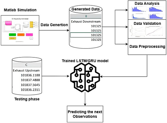
Figure 1.
The proposed method combining LSTM/GRU and simulated engine data for time-series prediction.
2.2. Modeling the Impact of EBP on Power Loss
Diesel engine performance is strongly influenced by EBP, impacting fuel efficiency, combustion stability, and emissions. Elevated backpressure impedes proper exhaust gas evacuation during the exhaust stroke, increasing the residual exhaust gas fraction within the combustion chamber. As illustrated in Figure 2 from [41], residual gases occupy cylinder volume that would otherwise be available for fresh air intake. Consequently, the proportion of fresh air entering the cylinder decreases, negatively influencing the air–fuel mixture quality.
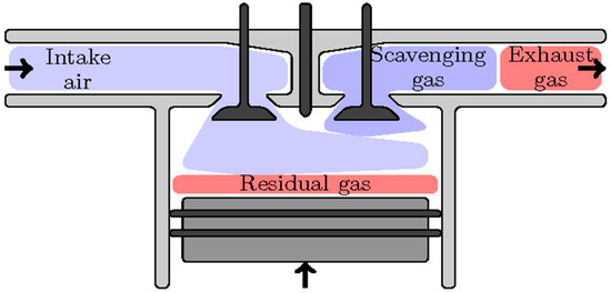
Figure 2.
Cylinder in exhaust phase with clear residual gas.
This elevated presence of residual exhaust gases diminishes combustion efficiency and reduces overall heat release during combustion. Moreover, the higher pressure within the exhaust manifold demands additional mechanical work by the piston during the exhaust phase, thereby directly lowering the net engine power output. Accurate modeling of this phenomenon is essential to quantify these losses and optimize diesel engine control strategies effectively.
To understand the impact of EBP on the work applied by the cylinder and, subsequently, on the effective work, it is essential to model various parameters using appropriate physical equations. The Indicated Mean Effective Pressure (IMEP) is a key metric representing the mean pressure that would produce the indicated work per cycle if it were applied uniformly in the cylinder [1]. Mathematically, it is expressed as:
where is indicated work per cycle (J), and is displaced cylinder volume (m3) Another central parameter to understand the efficiency of cylinder mixture before combustion is volumetric efficiency , it refers to the engine’s ability to admit fresh air into the cylinders [42], defined as:
where is the theorical admit air mass that is expressed by multiplication of air density and displaced cylinder volume. The is theorical one multiplied by volumetric efficiency. From the air–fuel ratio, the following relation is derived:
where represents the fuel mass and denotes the stoichiometric air–fuel ratio.
Two fundamental equations in thermodynamics and internal combustion engine performance analysis directly contribute to the analysis of power loss, as well as the modeling of the EBP effect, heat transfer, and work output (mechanical work). These equations are modeled as follows:
where represents the heat transfer results from the air fuel mixture combustion, and is the Lower Heating Value of the fuel.
where denotes the mechanical work produced from combustion, and represents the thermal efficiency.
Based on the previous analysis, the following conclusion can be drawn:
It can be inferred that a decrease in volumetric efficiency leads to a reduction in IMEP, directly affecting the power generated by the engine cylinder [1].
It is important to note that the net IMEP is impacted not only by volumetric efficiency but also, the pressure applied by the exhaust gas on the cylinder [1], the formula is presented by:
where PMEP denotes the Pumping Means Effective Pressure.
We relate indicated and brake mean effective pressures as:
where FMEP denotes mechanical (friction) losses and PMEP denotes pumping losses. For a four-stroke engine, BMEP links to brake torque T by:
With the total displaced volume. Effective (brake) power then follows from:
where n is engine speed in revolutions per second. Thus, given IMEP and model-based FMEP and PMEP, we obtain BMEP and the corresponding effective power.
2.3. Data Acquisition and Embedded System Development
2.3.1. System Overview
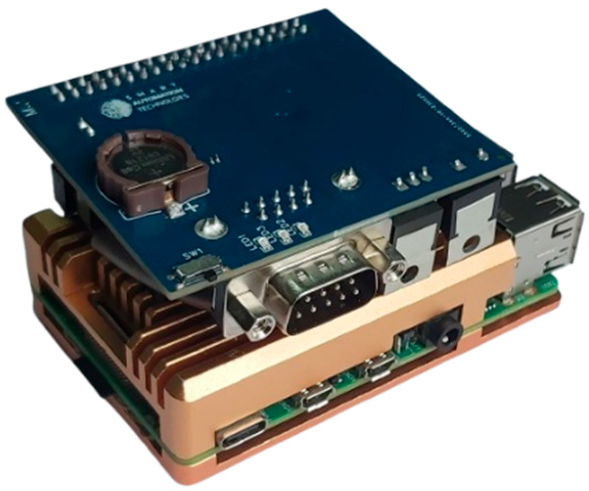
To enable real-time data acquisition from the vehicle’s CAN bus, an embedded system was developed to interface directly with the vehicle’s Electronic Control Units (ECUs). This system is designed to extract critical parameters necessary for EBP monitoring and predictive maintenance of diesel engines. The architecture consists of a Raspberry Pi 4 as the central processing unit, complemented by a custom-designed auxiliary (Printed Circuit Bord) PCB for power regulation and OBD2 communication. Figure 3 shows assembled system.

Figure 3.
Acquisition System.
2.3.2. Hardware Architecture
The hardware setup integrates a Raspberry Pi 4 Model B, manufactured by Raspberry Pi Foundation (Cambridge, UK), chosen for its optimal balance of processing power, energy efficiency, and affordability; the Pi handles data acquisition, real-time processing, and predictive analysis on-board. Its quad-core Cortex-A72 CPU (with up to 8 GB RAM) provides enough headroom for GRU/LSTM inference. Linux with SocketCAN gives stable, low-latency CAN I/O via the MCP2515 (manufacturer Microchip Technology, Chandler, AZ, USA) and TJA1050 (manufacturer NXP Semiconductors, Eindhoven, The Netherlands) CAN transceiver board. The mature toolchain (Python version 3.9.5, python-can version 3.3.3, ONNX version 1.8.1, TensorFlow Lite version 2.6.0) speeds deployment. Rich I/O—SPI for the CAN controller, GPIO/UART, USB 3.0 for fast logging or SSD, Gigabit Ethernet, and dual-band Wi-Fi for updates/telemetry—supports reliable in-vehicle operation. Low 5 V power simplifies integration, while SSD or industrial-grade SD cards, basic thermal management, and optional PREEMPT-RT improve robustness. Strong availability and community support further reduce cost and maintenance risk. To establish a stable communication channel with the vehicle’s CAN bus, a dedicated PCB (Smart Automation Technologies, Tangier, Morocco) was designed, incorporating:
- MCP2515 CAN Controller for handling CAN communication.
- TJA1050 CAN Transceiver for converting signals between the CAN bus and the microcontroller.
- Power regulation circuit to ensure stable voltage levels for seamless operation.
- DB9 connector interface for direct connection to the OBD2 port.
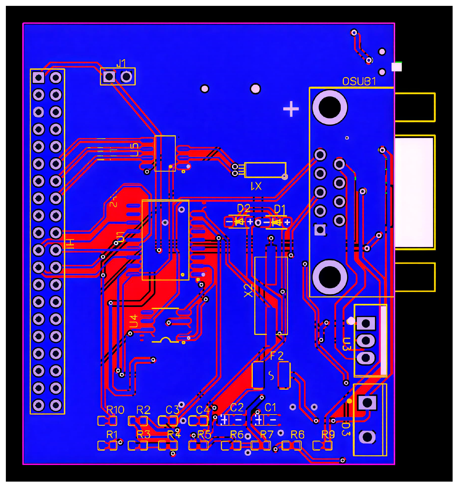
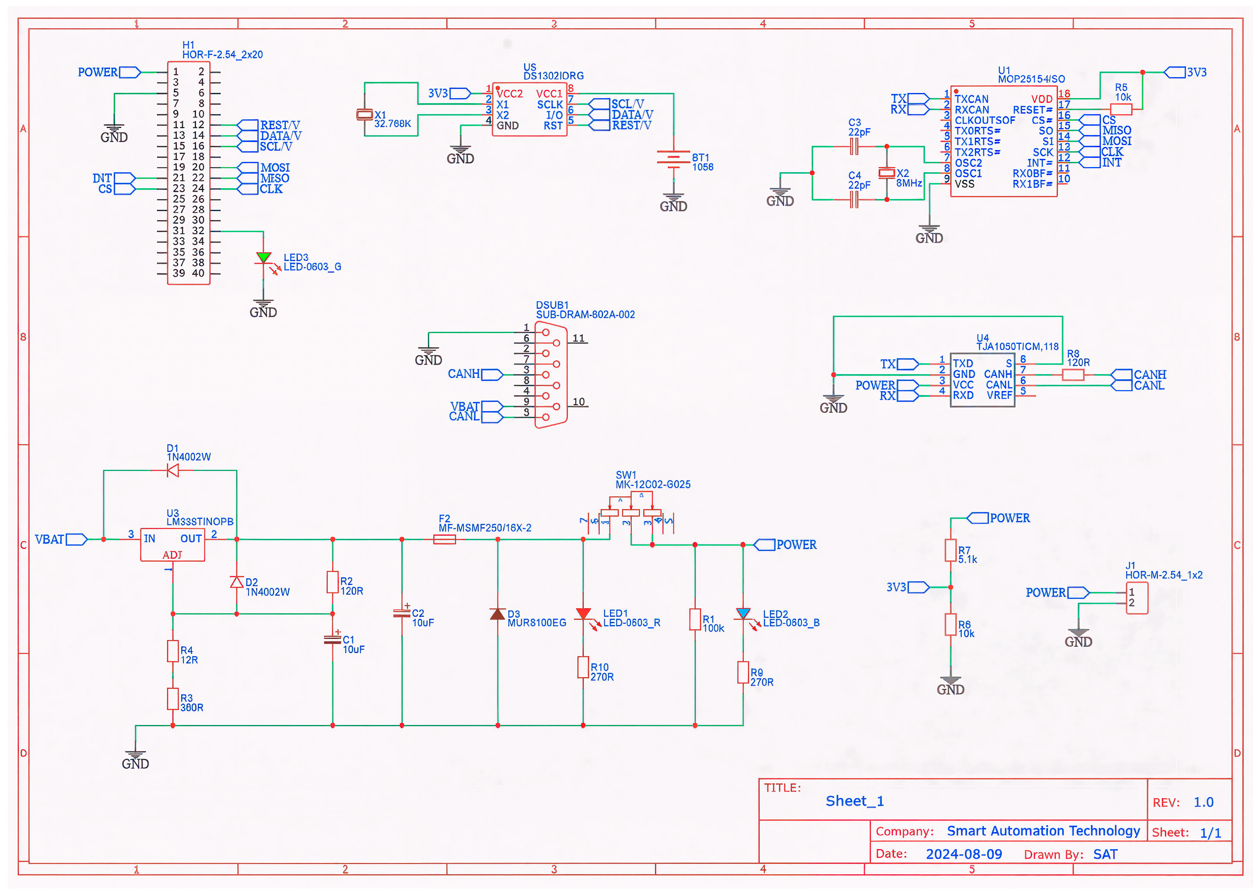
The PCB is shown in Figure 4, while the schematic in Figure 5 present a detailed view of the auxiliary card
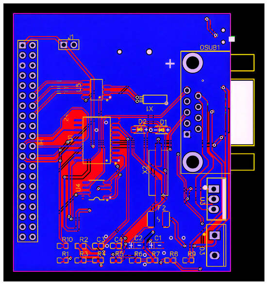
Figure 4.
Auxiliary Card Layout PCB.
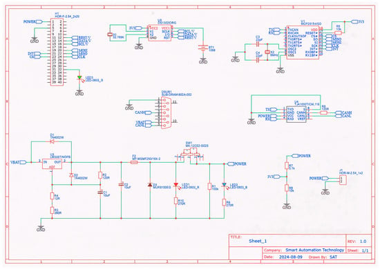
Figure 5.
Auxiliary Card Schematic.
2.3.3. Software Implementation
Python-can library, enabling direct interfacing with the CAN hardware. Raw CAN message decoding, where hexadecimal CAN frames are converted into meaningful engine parameters using DBC files. Real-time filtering and error handling, removing redundant or erroneous packets. Data storage and visualization, ensuring long-term logging and graphical representation of extracted parameters. The complete code, configurations, DBC files, and data will be made available on a GitHub repository upon the completion of the full integration of the work.
2.3.4. OBD2 Parameter Extraction and Decoding
To retrieve critical vehicle parameters, the system requests specific OBD2 PIDs, which are then processed to extract engine-related variables. The response from the ECU follows a standard hexadecimal structure, which is decoded into human-readable values. Figure 6 illustrates the bully CAN bus OBD2 protocol data row, an example of engine coolant temperature (PID 05) being successfully extracted from raw CAN messages.

Figure 6.
Decoded ready-to-use data.
To enhance real-time performance, the acquired CAN data is processed directly on the Raspberry Pi using an edge computing approach. The data is filtered, structured, and subsequently fed into the machine learning pipeline for predictive modeling. The final dataset is stored in a structured format, as illustrated in Figure 7, making it suitable for further analysis and model training.

Figure 7.
OBD2 Raw Data.
2.4. EBP Modeling and Synthetic Data Generation
2.4.1. Introduction to Powertrain Block Set
The Powertrain Blockset in MATLAB/Simulink is a specialized modeling and simulation library designed for automotive powertrain systems. It provides pre-built, customizable component models and comprehensive reference applications for various powertrain configurations, including Internal Combustion Engines (ICE), hybrid-electric, and fully electric vehicles [43].
Among these applications, the CIDynoRefApp, specifically models a diesel engine dynamometer setup, integrating detailed subsystems for intake and exhaust dynamics, turbocharging with VGT, EGR, and emissions characterization [44]. This model has been effectively utilized in scientific literature for systematically analyzing diesel engine performance and emissions, explicitly simulating variations in EBP, volumetric efficiency, and IMEP [45,46]. Consequently, it offers a robust, validated environment for research, calibration, and optimization of diesel powertrain control strategies.
2.4.2. Presentation of CID_Reference_Application
The provided diagram in Figure 8 represents a Simulink model of an Engine Dynamometer designed for engine performance simulation and testing. The model integrates three primary functional blocks: Calibration Controller, Engine System, and Dynamometer. The Calibration Controller manages the dynamometer and engine commands, providing adaptive control signals based on system calibration procedures. The Engine System simulates dynamic engine behavior, processing inputs such as Dynamometer Control (DynoCtrl) and environmental variables to produce outputs including torque and speed. The Dynamometer block simulates load conditions applied to the engine, reflecting realistic operation scenarios through controlled torque feedback. Performance data, including Engine Speed (EngSpd), Commanded Torque (TrqCmd), and Actual Engine Torque (EngTrq), is monitored and evaluated within the Performance Monitor block. Additional auxiliary blocks provide automated functionalities for executing mapping experiments, recalibrating the controller, and generating engine parameter mappings. Such integrated dynamometer models are widely adopted in automotive research, particularly in validating control algorithms, engine performance optimization, and predictive maintenance systems [47]. Table 2 presents a comparison between the features of the real-world engine and the simulated engine.
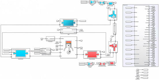
Figure 8.
Engine system bloc (generated using MATLAB Powertrain Blockset).

Table 2.
Comparison of real-world and simulated engine.
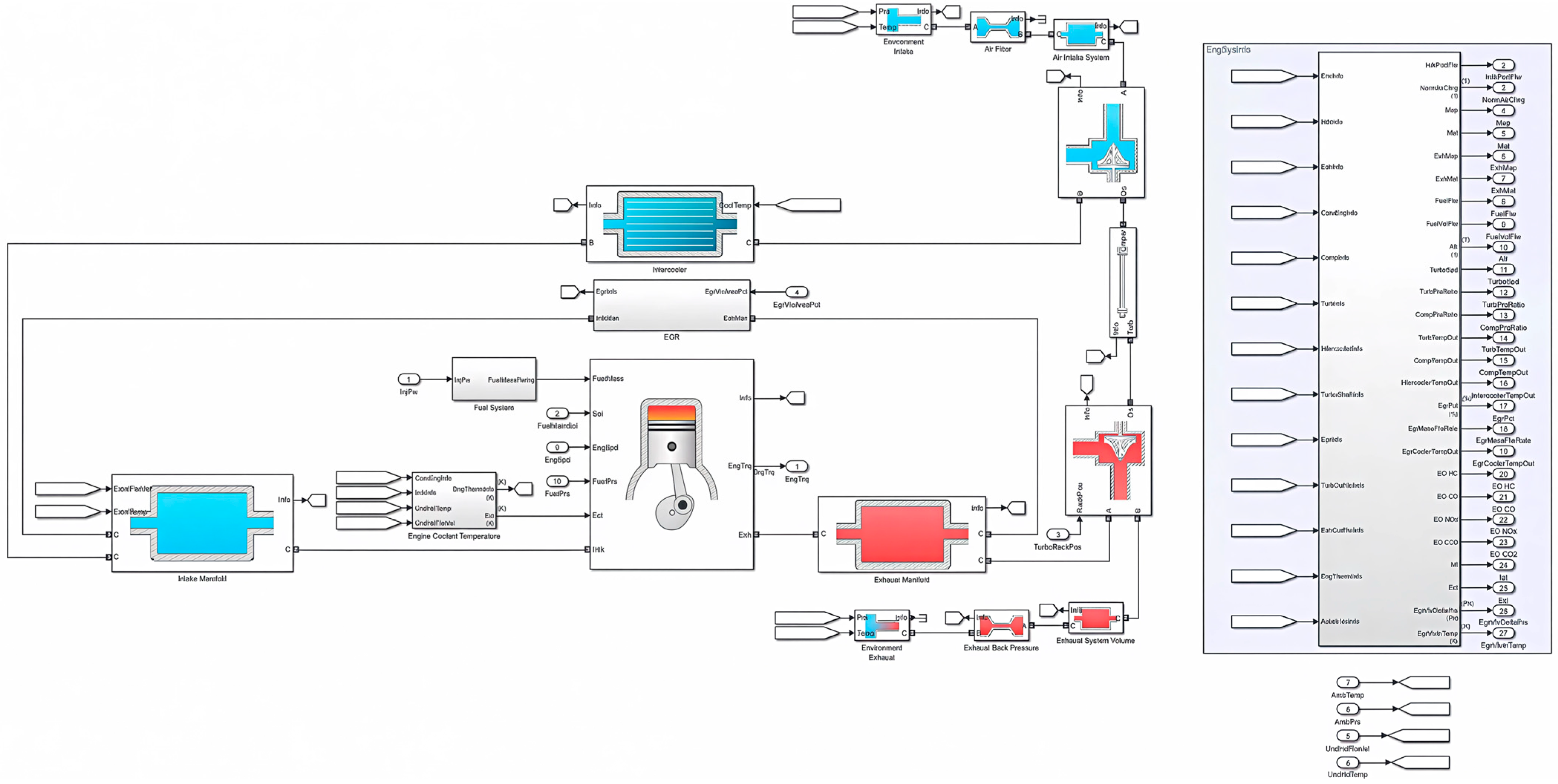
The provided diagram illustrates a comprehensive Simulink model for a detailed engine system simulation, particularly focusing on internal combustion engine components and their interactions. The central section features key subsystems such as the Intake Manifold, Intercooler, EGR, Engine Cylinder (combustion chamber), and Exhaust Manifold. Each subsystem represents specific physical processes: The Intake Manifold manages incoming airflow dynamics based on temperature and mass flow inputs; the Intercooler lowers intake charge temperature to improve efficiency; the EGR subsystem recirculates exhaust gases to reduce emissions; the Engine Cylinder simulates combustion processes translating fuel-air mixtures into torque output; and the Exhaust Manifold models exhaust gas dynamics post-combustion.
The model also integrates complementary blocks for environmental conditions, air filtration, turbocharging, and exhaust system dynamics. Outputs such as fuel mass, engine torque, and emissions parameters are systematically captured for monitoring and analysis. Such multidimensional modeling frameworks are critical in automotive engineering research for optimizing engine performance, enhancing emission control, and developing advanced predictive control strategies [1,2,48].
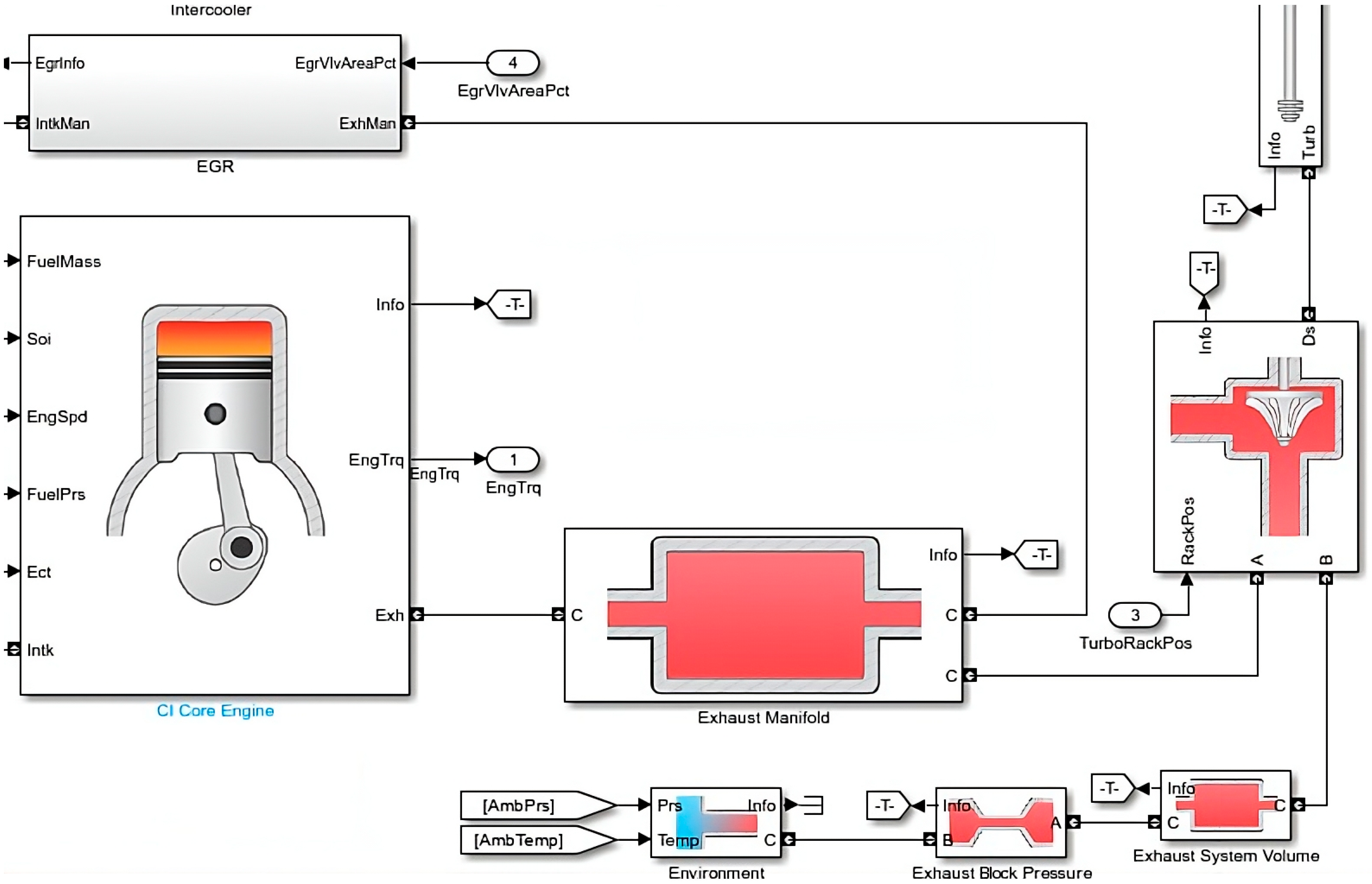
This Simulink subsystem Figure 9 represents the combustion and exhaust process of an internal combustion engine. The engine cylinder receives inputs such as fuel mass, engine speed, fuel pressure, and coolant temperature to simulate combustion dynamics, generating engine torque and exhaust gases. Post-combustion gases flow through the exhaust manifold, entering a turbocharger system for pressure and flow management, before being expelled via an exhaust system volume. Environmental conditions (pressure and temperature) also influence the exhaust dynamics. Such subsystems enable precise simulation of combustion efficiency, emission profiles, and turbocharger performance [1,48].
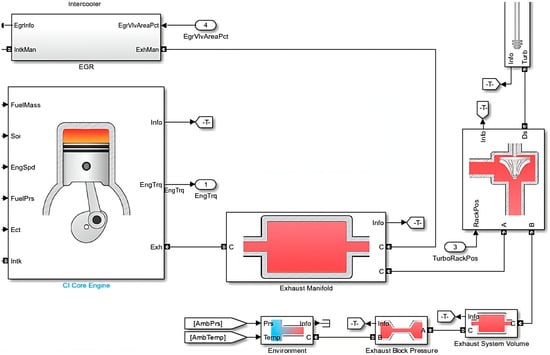
Figure 9.
CI engine: exhaust system part (generated using MATLAB Powertrain Blockset.).
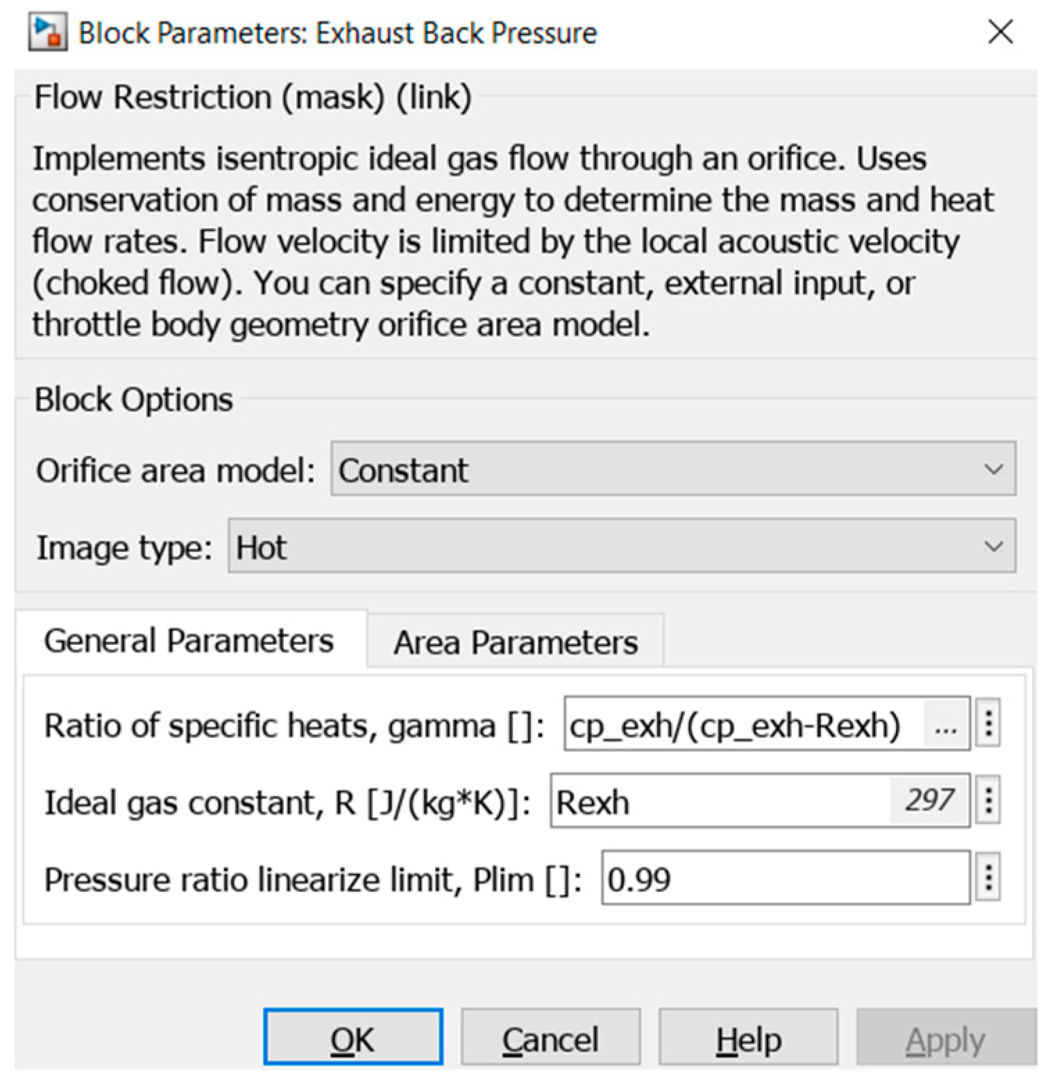
The model also integrates complementary blocks for environmental conditions, air filtration, turbocharging, and exhaust system dynamics. Outputs such as fuel mass, engine torque, and emissions parameters are systematically captured for monitoring and analysis. Such multidimensional modeling frameworks are critical in automotive engineering research for optimizing engine performance, enhancing emission control, and developing advanced predictive control strategies [1,2,48]. This Simulink subsystem Figure 9 represents the combustion and exhaust process of an internal combustion engine. The engine cylinder receives inputs such as fuel mass, engine speed, fuel pressure, and coolant temperature to simulate combustion dynamics, generating engine torque and exhaust gases. Post-combustion gases flow through the exhaust manifold, entering a turbocharger system for pressure and flow management, before being expelled via an exhaust system volume. Environmental conditions (pressure and temperature) also influence the exhaust dynamics. Such subsystems enable precise simulation of combustion efficiency, emission profiles, and turbocharger performance [1,48]. The window in Figure 10 presents a parameter configuration panel for the “EBP” block in Simulink, which models a flow restriction through an orifice using an isentropic ideal gas flow assumption. This block calculates mass flow and pressure drop by applying conservation of mass and energy, with flow velocity constrained by the local acoustic velocity, characterizing choked flow conditions. Key parameters include the ratio of specific heats (gamma), ideal gas constant (R), and pressure-ratio linearization limit (Plim), defining the conditions under which linearization is valid. Such modeling is essential in analyzing exhaust gas dynamics, accurately predicting engine backpressure effects on performance and emissions.

Figure 10.
Exhaust backpressure configuration panel (generated using MATLAB Powertrain Blockset).
2.5. Data Generation
In the context of engine performance modeling and analysis, the EBP block in Simulink plays a critical role in simulating the flow restriction in the exhaust system. This block models the isentropic ideal gas flow through an orifice, ensuring conservation of mass and energy to determine the mass flow rate and thermal behavior of exhaust gases. One of the most influential parameters within this block is the Plim, which MATLAB allows to be modified within the range of 0.99 to 0.855. Adjusting this parameter allows for the simulation of both normal and abnormal engine operating conditions by modifying the backpressure levels, which directly affect engine efficiency, emissions, and performance.
To generate meaningful synthetic data for analysis, a systematic approach is required. The first step is to vary the Plim parameter systematically, starting from its highest value (0.99), which represents an optimal flow condition with minimal flow restriction, down to lower values (0.855), simulating cases where backpressure increases due to clogging, turbocharger failure, or exhaust system blockages. Higher backpressure conditions are typically associated with incomplete combustion, reduced power output, and increased fuel consumption, making them critical scenarios to study. By adjusting Plim, a dataset can be generated that encompasses a full range of engine operating conditions, from optimal exhaust flow to extreme restriction scenarios.
To collect this data, Simulink’s Bus Creator is employed to organize and store multiple signals into a single data stream, ensuring efficient logging of all relevant engine parameters. The key parameters that characterize EBP and its effects on engine performance include exhaust pressures, engine speed, turbocharger behavior, fuel consumption, and emissions-related variables. These parameters provide essential insights into how varying backpressure levels influence torque output, combustion efficiency, and emission formation. A structured overview of the most critical parameters influencing EBP is provided in Table 3.

Table 3.
Key Parameters Influencing Exhaust Backpressure.
The importance of data variability in this experiment cannot be overstated. A diverse dataset enables robust model training for predictive analytics and anomaly detection, particularly in applications related to predictive maintenance and fault diagnosis in engines. By varying Plim, the dataset is ensured to represent both healthy engine conditions and faulty scenarios, thereby making it valuable for machine learning models, statistical analysis, and control system optimization. Capturing abnormal situations allows for the development of early fault detection algorithms, which can be applied in real-time monitoring systems to predict failures before they escalate into costly breakdowns. Additionally, this approach supports the design of adaptive engine controllers that can adjust parameters dynamically based on backpressure feedback.
In the simulation, PMEP is available from the gas-exchange model. Mechanical losses are represented via friction mean effective pressure (FMEP) from the engine friction sub-model (speed/load dependent). We compute BMEP as , then obtain brake torque and effective power using the relations above.
2.6. Data Analysis
2.6.1. Data Distribution Analysis
Understanding the distribution of key variables is essential for assessing the variability and behavior of exhaust system parameters [49]. This analysis provides insights into underlying data trends, identifies possible asymmetries or extreme values, and helps optimize predictive maintenance strategies using deep learning techniques [50]. The study focuses on six critical features: Exhaust Upstream Pressure, Exhaust Downstream Pressure, and the emissions of NOx, CO, CO2, and Hydrocarbons (HC). The objective is to evaluate whether these parameters follow a normal distribution and determine their implications for deep learning-based anomaly detection and fault prediction.
The Exhaust Upstream Pressure, as shown in Figure 11 distribution reveals a right-skewed pattern, with values concentrated around 105,000 Pa and an extended tail beyond 120,000 Pa. This asymmetry suggests that the engine operates predominantly within a stable pressure range but occasionally experiences pressure peaks due to increased engine load, turbocharger activation, or EBP buildup. Additionally, local peaks indicate multimodal characteristics, likely representing different engine operating conditions, such as low-load, mid-load, and high-load states. This multimodal behavior highlights the need for deep learning models that can capture complex, nonlinear relationships rather than assuming a single distribution across all conditions.

Figure 11.
Histogram and Density Analysis of Exhaust Upstream and Downstream Pressure (Pa).
The Exhaust Downstream Pressure shows an extreme right-skew, with a sharp peak at 101,325 Pa and a long tail extending beyond 102,000 Pa. This suggests that downstream pressure remains relatively stable in most cases but experiences occasional transient fluctuations, possibly due to EGR activation, changes in exhaust flow, or system inefficiencies. Given this distribution, traditional statistical models assuming normality may not be effective, making deep learning-based models, such as LSTMs, more suitable for predicting pressure deviations and identifying system faults.
The analysis of emissions further illustrated in Figure 12 confirms the non-normal nature of the dataset. Tailpipe NOx Emissions exhibit a strong right-skew, with most values close to zero and a long tail extending towards higher concentrations. NOx formation is highly dependent on combustion conditions, and sharp peaks in NOx levels may indicate high-load events, inefficient EGR operation, or turbocharger variations. Similarly, Tailpipe CO Emissions display a multimodal distribution, with distinct peaks at different concentration levels, suggesting that CO production is significantly affected by combustion dynamics and air–fuel ratio fluctuations. These variations reinforce the need for deep learning models that can dynamically adjust to different operating regimes rather than relying on predefined statistical assumptions.
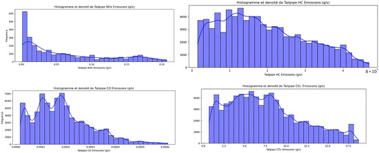
Figure 12.
Histogram and Density Analysis of Tailpipe Emissions (CO, HC, NOx, CO2).
Tailpipe CO2 Emissions demonstrate a relatively broad distribution with slight skewness, reflecting variations in engine efficiency, air–fuel ratio regulation, and transient load conditions. Since CO2 is directly linked to fuel combustion, monitoring its fluctuations can help assess engine performance anomalies. Finally, Tailpipe HC Emissions show a spread of values, with asymmetric tendencies, indicating changes in combustion efficiency and potential fuel injection issues.
These findings indicate that none of the studied variables follow a normal distribution, which is crucial for deep learning-based predictive maintenance strategies. The presence of asymmetries, multimodal distributions, and long tails suggests that conventional linear models may not be suitable. Instead, deep learning architectures such as Recurrent Neural Networks (RNNs) should be considered for capturing the complex patterns present in the exhaust system data. Additionally, feature transformations such as log-scaling, normalization, or embedding techniques may improve the representation of skewed data, enhancing model performance.
The strong variability in emissions and pressure values also suggests that a segmentation-based approach, where the data is categorized into different operating states, may improve prediction accuracy. Future work should focus on feature engineering, real-time monitoring integration, and deep learning model optimization to enhance fault detection and predictive maintenance capabilities in exhaust systems.
2.6.2. Analysis of Upstream Exhaust Backpressure Variations
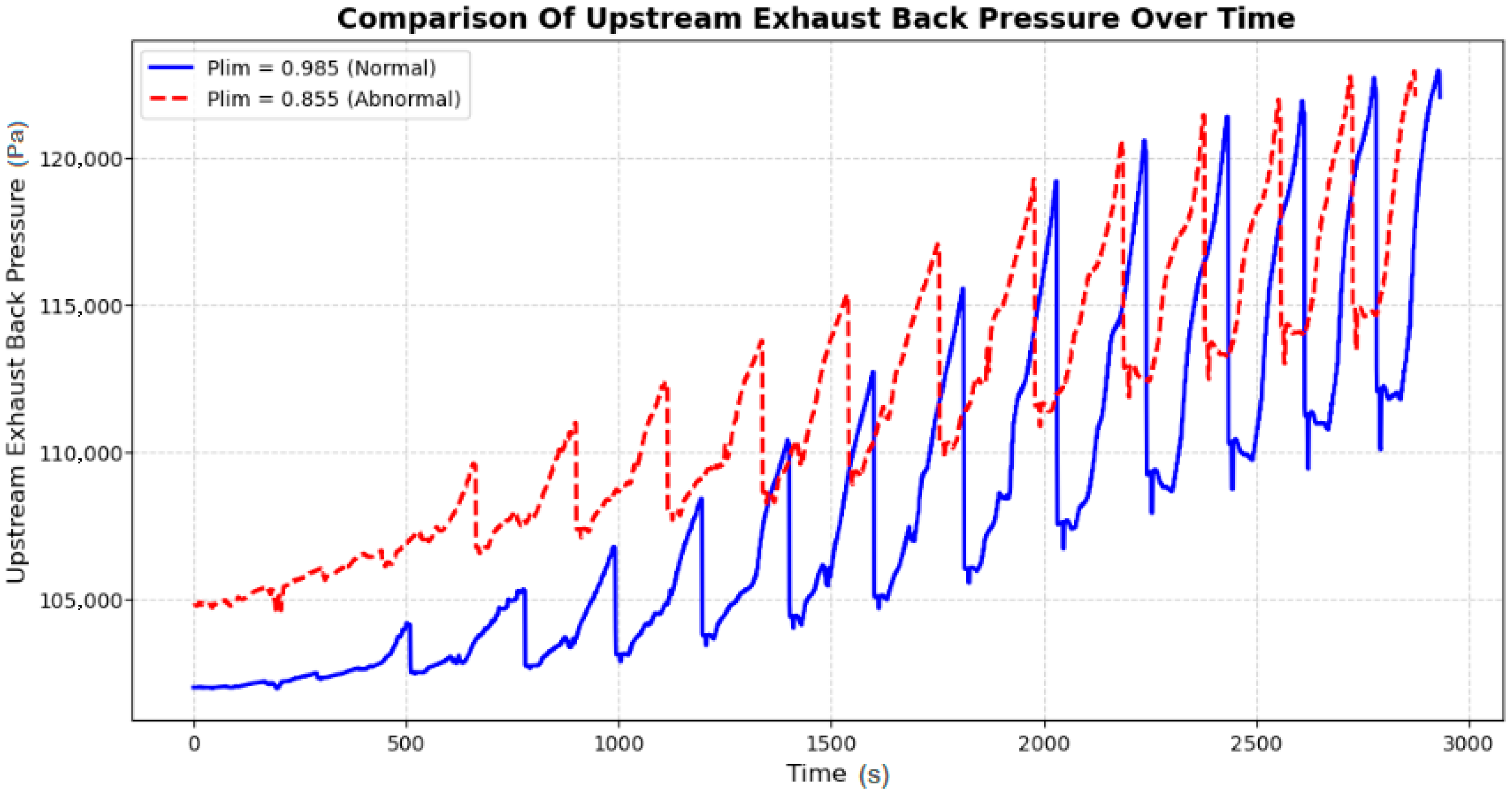
The graph presented in Figure 13 illustrates the comparison of upstream exhaust backpressure over time for two selected values of the pressure-ratio linearization limit (Plim), a parameter that governs the restriction of exhaust flow in the Simulink engine model. The solid blue curve represents the normal operating condition with Plim = 0.99, while the dashed red curve corresponds to an abnormal scenario with Plim = 0.855. These values were chosen to reflect, respectively, a nominal condition and a degraded condition with increased exhaust resistance. The upper value (0.99) represents a healthy system with minimal flow restriction, while the lower value (0.855) is the minimum that can be reliably applied in Simulink without compromising simulation stability. Both lie within the permitted range of the block’s configuration and allow the simulation of meaningful exhaust degradation scenarios without altering the system geometry.

Figure 13.
Comparison of upstream exhaust backpressure over time.
The x-axis represents time (s), and the y-axis represents upstream exhaust backpressure (Pa), measured at the exhaust manifold before the turbine and after the combustion process. The purpose of this comparison is to evaluate the impact of exhaust flow restriction on backpressure and its implications for engine performance, turbocharger efficiency, and emissions control.
A key observation from Figure 6 is the distinct difference in backpressure behavior between the two conditions. When A key observation from Figure 13 is the distinct difference in backpressure behavior between the two conditions. When Plim = 0.99 (blue curve), the upstream exhaust backpressure remains consistently lower, with a periodic oscillatory pattern corresponding to the engine’s operational cycles. This indicates efficient scavenging of exhaust gases, allowing for a smooth flow with minimal resistance. In contrast, when Plim = 0.855 (red dashed curve), the upstream pressure is consistently higher, showing a greater buildup over time. The increased pressure spikes indicate a significant restriction in the exhaust flow, leading to elevated resistance against gas expulsion from the combustion chambers. This higher backpressure negatively impacts engine performance by reducing volumetric efficiency, increasing pumping losses, and altering combustion characteristics.
The periodic spikes in backpressure observed in both cases suggest a direct correlation with engine cycles and turbocharger behavior. However, in the abnormal condition (Plim = 0.855), the amplified peaks imply higher resistance to exhaust flow, forcing the engine to work harder to evacuate combustion gases. This results in higher exhaust gas temperatures, reduced turbocharger efficiency, and an increase in emissions due to incomplete combustion. The selected values of Plim thus provide a numerically stable and physically representative way to explore the dynamics of exhaust system degradation within the simulation framework.
Further analysis of the rate of change of upstream EBP (derivative analysis) is provided in Figure 14, which highlights the fluctuations in the rate at which pressure changes over time. This derivative analysis is crucial for identifying system stability, transient pressure spikes, and potential anomalies in exhaust flow behavior. The x-axis represents time (s), while the y-axis represents the rate of change of upstream EBP (Pa/s). The blue solid line (Plim = 0.985) represents the normal case, while the red dashed line (Plim = 0.855) represents the abnormal condition.
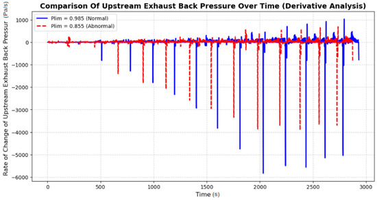
Figure 14.
Rate of Change of Upstream Exhaust Backpressure Over Time (Derivative Analysis).
The key observation from Figure 14 is that the normal operating condition (Plim = 0.985) exhibits controlled, moderate fluctuations in the rate of pressure change, meaning that pressure variations are more stable and predictable. However, in the abnormal case (Plim = 0.855), the rate of change exhibits frequent, extreme downward spikes, indicating sudden drops in backpressure that suggest flow disruptions and instability. These sharp fluctuations could be linked to exhaust flow turbulence, inefficient gas scavenging, and pressure surges that negatively impact the turbocharger response and overall engine operation.
2.6.3. Analysis of Pressure Variations
Figure 15 adapted from [24]. Effect of increasing exhaust backpressure on key pressures in a turbocharged engine: compressor inlet (solid, ≈1 bar, near-ambient), compressor outlet/boost (dashed, decreases with backpressure), turbine outlet (dash-dotted, increases with backpressure), and turbine inlet (dotted, slight dip at low backpressure followed by a rise). The rise in turbine-side pressures reflects growing exhaust restriction and pumping losses, while the drop in boost indicates reduced turbocharger effectiveness under higher backpressure.
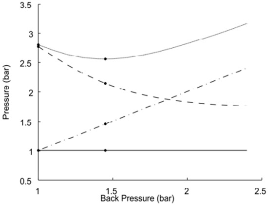
Figure 15.
Effect of Increasing Backpressure on Compressor and Turbine Pressures.
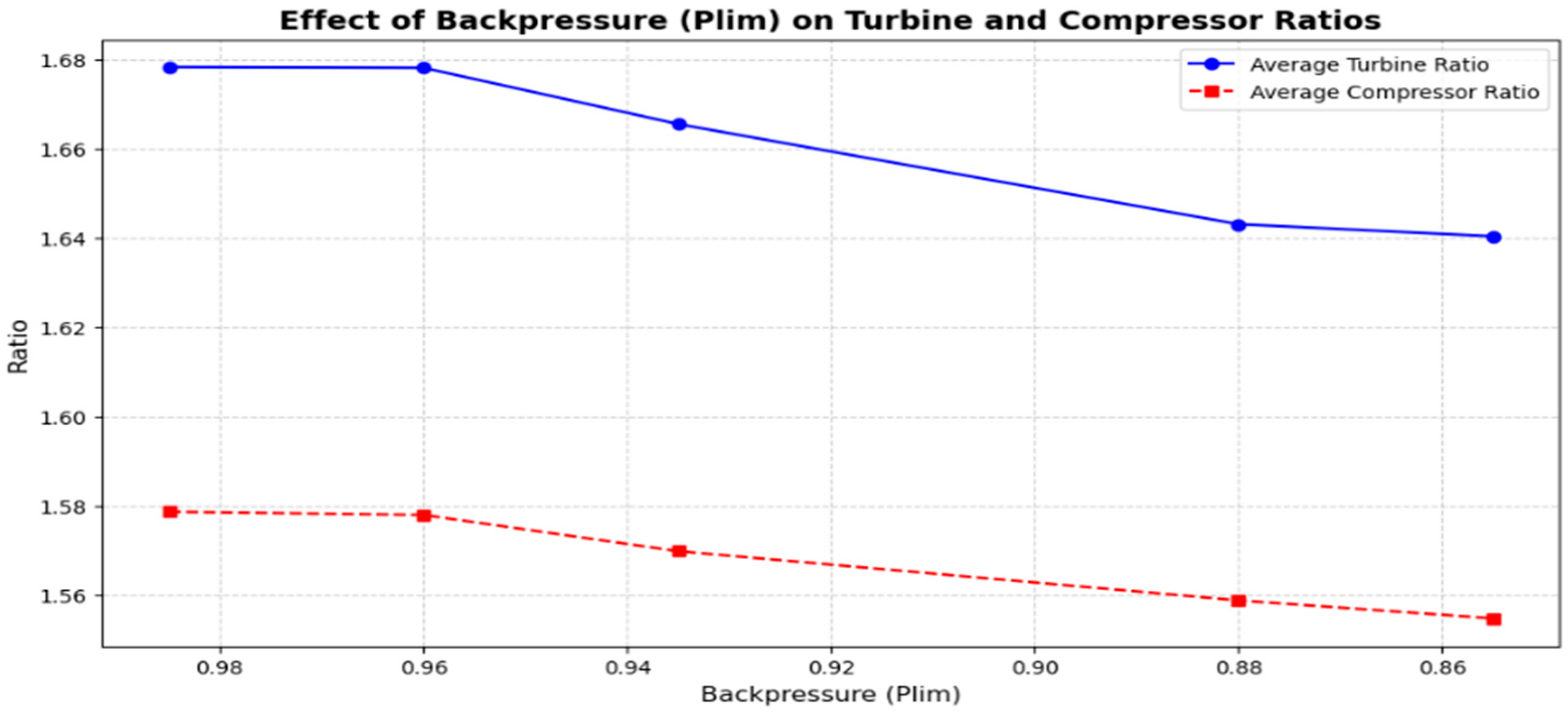
To assess the realism of our synthetic data, Figure 16 presents the variation in average turbine and compressor pressure ratios in response to increasing backpressure, implemented in our model via decreasing values of the pressure-ratio linearization limit (Plim). As Plim decreases from 0.99 to 0.86, the turbine pressure ratio drops from 1.68 to 1.63, while the compressor pressure ratio decreases from 1.58 to 1.555. These trends align with the physical behavior observed in [24], where turbine outlet pressure increases and compressor outlet pressure decreases under elevated backpressure conditions. Although our model uses normalized pressure ratios and [24] reports absolute pressures in bar, the observed dynamics and direction of change are consistent. This comparative analysis supports the validity of the synthetic dataset generated using the Simulink-based model and confirms its ability to replicate the impact of exhaust flow restriction on turbocharger performance. The combined interpretation of Figure 15 and Figure 16 demonstrate that increased backpressure leads to reduced turbine expansion efficiency and compressor effectiveness, ultimately resulting in higher engine workload, increased fuel consumption, and degraded performance.

Figure 16.
Influence of backpressure on turbine and compressor pressure ratios.
2.6.4. Engine Power Analysis
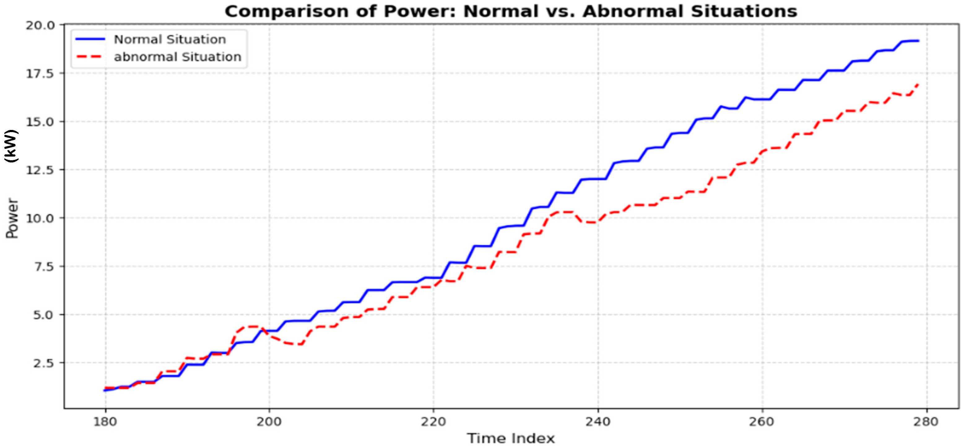
Figure 17 clearly demonstrates the impact of increasing EBP on engine power output. The graph compares two scenarios: the normal operating condition (solid blue line) and an increased backpressure scenario (dashed red line) after modifying the Plim parameter. It is evident that the increased backpressure scenario leads to a noticeable power loss, with the power curve consistently below the normal condition across the analyzed time period. This result highlights how elevated backpressure negatively affects engine performance, emphasizing the importance of maintaining optimal exhaust conditions to maximize efficiency and minimize power losses.
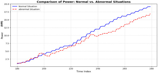
Figure 17.
Comparison of Power Under Normal and Increased Backpressure Conditions.
2.7. Model Architectures
2.7.1. LSTM Cell Structure
LSTM networks [51,52] are designed to enhance the short-term memory capacity of RNNs by integrating long-term memory states, commonly known as cell states [52,53]. The internal structure of an LSTM cell consists of three main gates: the input gate, output gate, and forget gate. These gates regulate the flow of information, allowing the network to retain or discard past information as needed [54].
The process begins, as illustrated in Figure 18, with the forget gate, which determines whether to retain or discard information from the previous cell state, denoted as . This decision is based on the current input data and the previous hidden state , both of which are processed through a sigmoid activation function. The output of the forget gate, , ranges between 0 and 1 and is computed as:
where represents the weight matrices of the forget gate, and denotes the bias term. The sigmoid function used in this computation is given by:
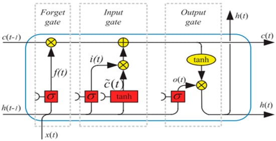
Figure 18.
Architecture of LSTM.
Next, the input gate plays a crucial role in updating the memory state. It first generates a candidate memory state, , by applying the hyperbolic tangent (tanh) activation function to the input and the previous hidden state :
The tanh function is defined as:
Simultaneously, the input gate determines which parts of this candidate memory state should be retained by computing the input state :
Using these values, the memory cell is updated as follows:
Finally, the updated hidden state is determined by the output gate. The output state, , is first calculated using a sigmoid activation function:
The new hidden state is then obtained by applying the tanh function to the updated memory cell state , followed by an element-wise multiplication with the output state:
This gated structure allows LSTMs to effectively manage long-term dependencies, mitigating the vanishing gradient problem that traditional RNNs face.
2.7.2. GRU Cell Structure
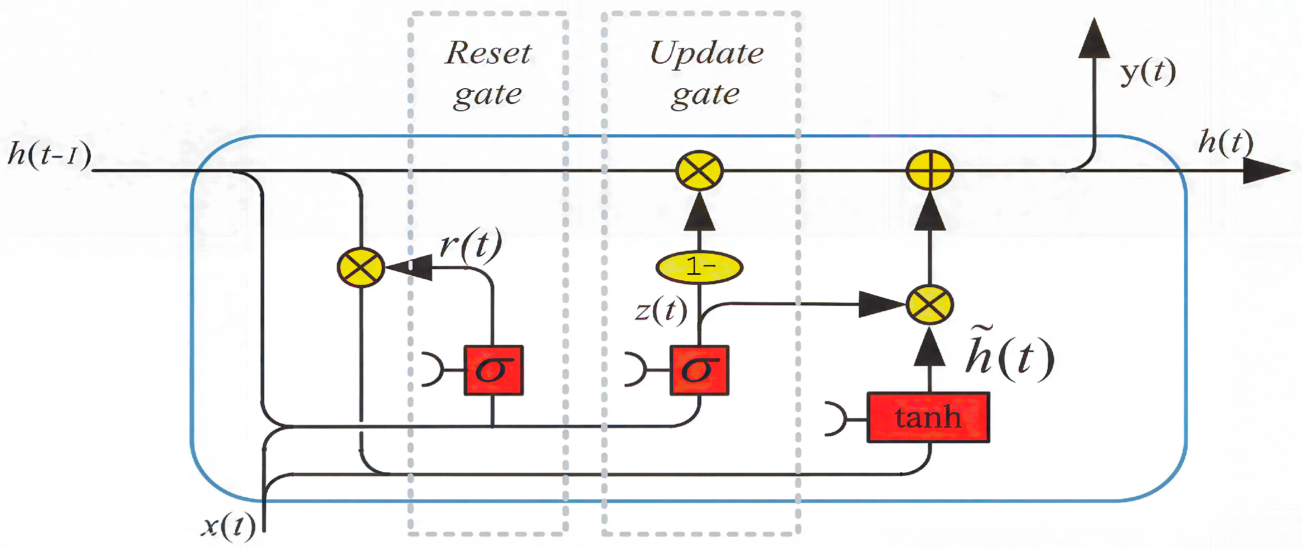
The GRU RNN [55] simplifies the LSTM model, as can be observed in Figure 19, by reducing the number of gating signals from three to two, update gate and Reset gate . The GRU was introduced by [56].

Figure 19.
GRU cell architecture.
The GRU updates its hidden state using the following equations:
With the two gates presented as:
It can be observed that the GRU RNN Equations (16) and (17) are similar to the LSTM RNN (13) and (14), but with fewer external gating signals in the interpolation Equation (16). This reduction removes one gating signal and its associated parameters. Further details are provided in the original source and the references cited therein.
In essence, the GRU RNN has a three-fold increase in parameters compared to the simple RNN. Specifically, the total number of parameters PGRU is given by:
It can be observed that the GRU RNN Equations (16) and (17) are similar to the LSTM RNN Equations (13) and (14), however with less external gating signal in the interpolation Equation (16). This saves one gating signal and the associated parameters. Further details are deferred to the original source and the references cited therein. In essence, the GRU RNN has a 3-fold increase in parameters in comparison to the simple RNN. In various studies, e.g., in [55] and the references therein, it has been noted that GRU RNN is comparable to, or even outperforms, the LSTM in most cases. Moreover, there are other reduced gated RNNs, see [54,57], e.g., the Minimal Gated Unit (MGU) RNN, where only one gate equation is used and it is reported that this (MGU) RNN performance is comparable to the GRU RNN, and by inference, to the LSTM RNN.
2.8. Dataset and Preprocessing
2.8.1. Experimental Setup
This section outlines the preprocessing, sequence construction, and training protocol used to develop recurrent models for predictive maintenance on engine performance data.
To ensure numerical stability and improve model convergence, standardization [58] was applied to all features. Each variable was transformed using z-score normalization [59], where the mean was subtracted, and the result was divided by the standard deviation, as described in (21):
where μ is the mean and σ is the standard deviation of the respective feature. This transformation ensures that all features have a mean of zero and a standard deviation of one, reducing the impact of scale differences between variables.
To preserve temporal order and avoid data leakage, the dataset was split chronologically into training (80%) and testing (20%) subsets [60]. The training set was used for model optimization, while the test set was reserved for performance evaluation, ensuring that the models were assessed on unseen data to prevent overfitting. Additionally, any missing values or anomalies were handled appropriately to maintain data integrity.
We selected a sequence length of 30 timesteps based on empirical testing. This length provided a good balance between capturing relevant temporal patterns in engine behavior and maintaining computational efficiency. Shorter sequences lost context, while longer ones added complexity without improving accuracy.
Since the output variable was continuous, no manual data labeling was required. However, we ensured that labels were correctly aligned with the input sequences during the sequence generation phase. A sliding window approach was used to generate overlapping input samples, increasing the training density and improving the model’s ability to generalize.
This preprocessed dataset served as the input for both LSTM and GRU models, allowing for a comparative study of their effectiveness in capturing temporal dependencies in engine performance data.
2.8.2. Training Configuration
The training of the LSTM and GRU models was conducted using a structured hyperparameter search to optimize performance [61,62]. The models were designed with a two-layer recurrent architecture, where hyperparameters such as the number of units, activation functions, dropout rates, learning rates, and batch sizes were systematically varied. The training was performed using the Adam optimizer, with validation loss as the optimization objective.
A grid search approach [62] with 20 trials was employed to explore different hyperparameter combinations, with each configuration executed twice to reduce performance variance. The validation loss was selected as the optimization objective to prevent overfitting and ensure model generalization.
Table 4 presents the set of hyperparameters considered for fine-tuning.

Table 4.
Hyperparameter fine-tuning.
The models were trained for 50 epochs with a batch size of 64. The Adam optimizer was chosen for its adaptive learning rate adjustments, which improve convergence speed. The final model selection was based on the configuration yielding the lowest validation loss.
The performance of the LSTM and GRU models was evaluated using four common metrics: Mean Absolute Error (MAE) [63], Mean Squared Error (MSE) [64], Root Mean Squared Error (RMSE) [63], and the R2 score [65]. These metrics are crucial for determining how well the models make predictions and how closely they match the actual values. Table 5 provides a comparison of the performance of the LSTM and GRU.

Table 5.
Comparative Performance Metrics of LSTM and GRU Models.
After evaluating the performance of both the LSTM and GRU models using key metrics, it is evident that GRU outperforms LSTM in terms of predictive accuracy and robustness. The GRU model achieves a Mean Absolute Error (MAE) of 0.0131, representing a 75.4% reduction compared to LSTM’s MAE of 0.0532. This indicates that GRU’s predictions are, on average, much closer to the actual values. Similarly, the Mean Squared Error (MSE) for GRU is 0.0011, which is a 94.0% decrease from the 0.0184 observed for LSTM, reflecting GRU’s enhanced capacity to minimize large deviations and better handle outliers. The Root Mean Squared Error (RMSE), which reflects the standard deviation of the prediction errors, is also significantly lower for GRU (0.0328) compared to LSTM (0.1358), amounting to a 75.8% improvement. These consistent reductions across all error metrics underline the GRU model’s superior generalization ability and stability, especially when dealing with time series data.
Although LSTM achieves a marginally higher R2 score (0.9817 vs. 0.9791), suggesting it explains a slightly greater proportion of the variance in the target variable, this difference is statistically negligible when considered alongside the substantial reductions in MAE, MSE, and RMSE. In fact, the slight decrease in R2 for GRU can be attributed to its tighter predictions around the mean, which result in minimal variance but significantly reduced absolute and squared errors. Overall, the findings confirm that GRU provides more accurate, stable, and practically meaningful predictions than LSTM, thereby justifying its adoption in the proposed predictive maintenance framework.
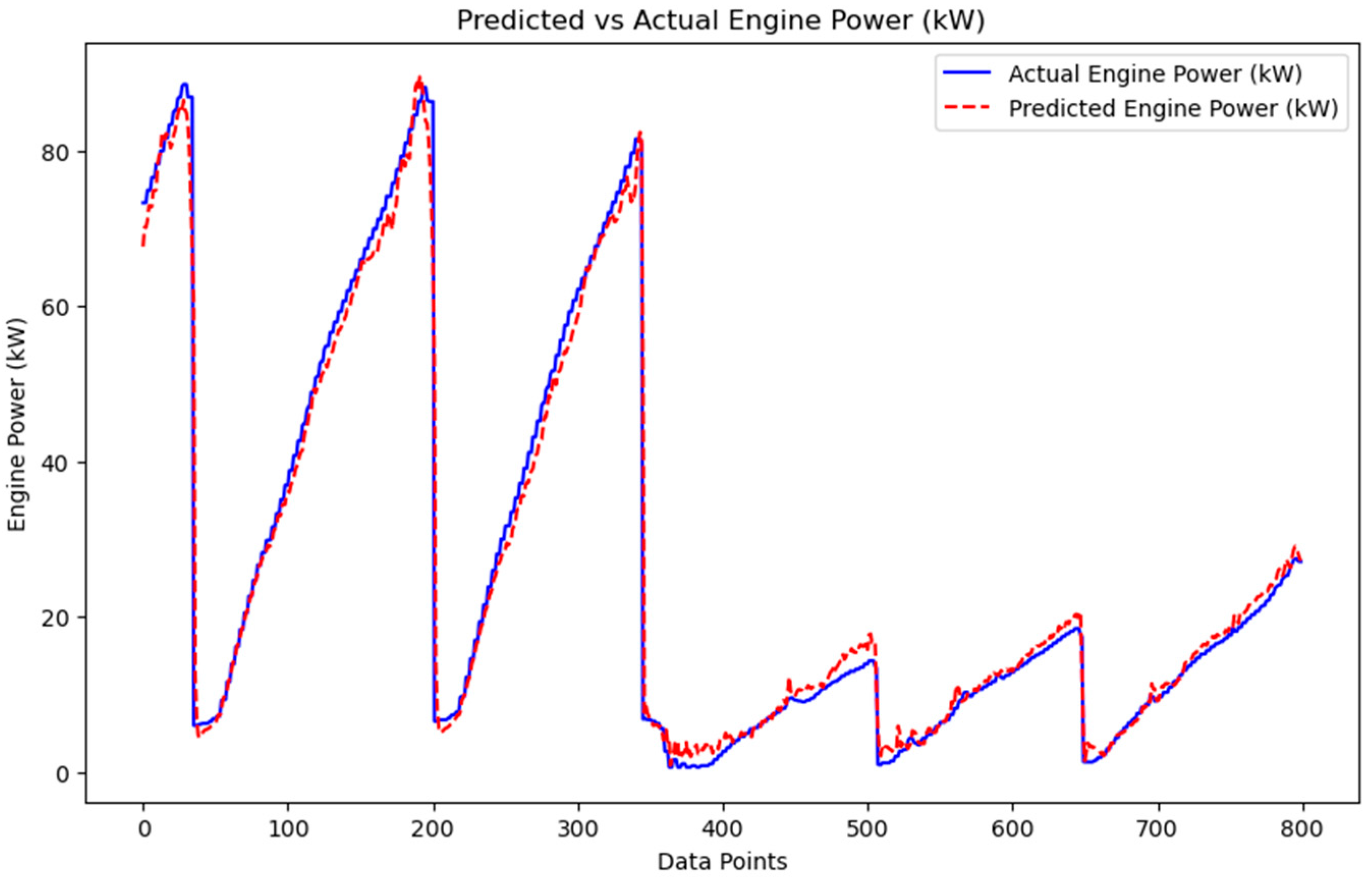
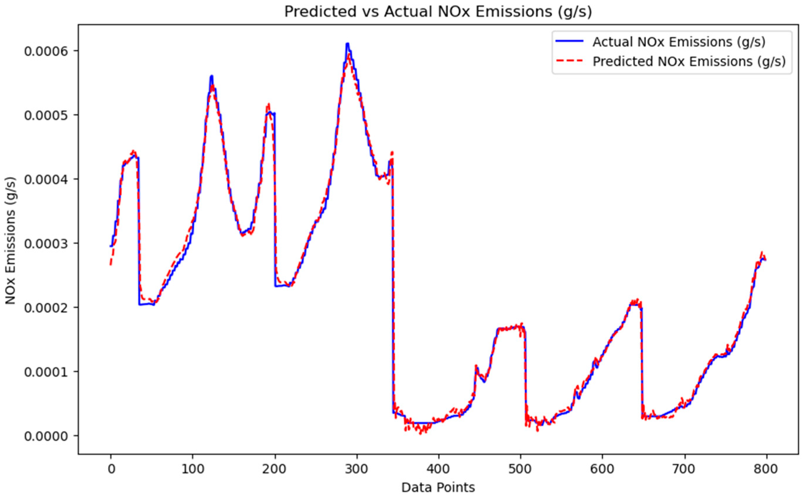
The plots in Figure 20 and Figure 21 compare the predicted and actual values for engine power (kW) and NOx emissions (g/s), showing how closely the GRU model predictions align with the true values over time.

Figure 20.
Predicted vs. Actual Engine Power (kW).

Figure 21.
Predicted vs. Actual NOx Emissions (g/s).
3. Discussion
This study aimed to develop an embedded system for vehicle data acquisition via OBD2, model the engine performance using MATLAB, and apply deep learning techniques to predict power loss caused by exhaust gas backpressure. The work progressed in three distinct phases: first, the development of an embedded system to acquire and preprocess vehicle data; second, the modeling of engine performance and powertrain parameters using MATLAB’s Powertrain Blockset; and third, the application of deep learning algorithms (LSTM and GRU) to predict engine states based on the generated data.
The following discussion provides an analysis of the results from each phase, comparing the generated data with established theoretical expectations and evaluating the performance of the deep learning models. This includes an exploration of the observed behaviors, the effectiveness of the modeling approach, and the performance of the predictive models in terms of accuracy and reliability.
In the first phase, the embedded system was developed to acquire vehicle data via the OBD2 protocol. This system enabled the decoding of data frames related to engine parameters, such as pressure and temperature sensors. These frames were preprocessed to make them compatible with the AI models used for predicting power loss due to exhaust gas backpressure.
The second phase focused on using MATLAB, specifically the “Powertrain Blockset,” to model the engine and its associated systems. Using an existing example (“CI Dyno Reference Application”), sensor data relevant to the powertrain, including pressure and temperature sensors, was generated. Modification of the EBP orifice size enabled the observation of how variations in backpressure influence engine performance.
The trends observed in the results, particularly the increase in power loss with decreasing orifice size, aligned with theoretical expectations. However, differences in specific values, such as turbine pressures and the turbine ratio, were observed. These discrepancies can be attributed to variations in the specifications and configurations of the engine models compared to the simulation setup used in this study.
Finally, in the third phase, two deep learning models were developed and trained to predict the engine state based on the generated data. LSTM and GRU models were selected for their efficiency in handling time-series data. After training the models on the generated data, a comparative study was conducted to evaluate the performance of both models using the following metrics:
- MAE: GRU = 0.0131, LSTM = 0.0532
- MSE: GRU = 0.0011, LSTM = 0.0184
- R2 Score: GRU = 0.9791, LSTM = 0.9817
While the LSTM model showed a slightly better performance in terms of R2 Score, the GRU model outperformed LSTM in MAE and MSE, with overall lower errors. This result highlights the effectiveness of GRU in modeling this type of problem, where capturing long-term temporal relationships is crucial, but without the complexity of the LSTM model. As a result, the use of GRU is recommended for this application due to its ability to provide more accurate predictions.
Our validation relies on synthetic faults because current real OBD-II/CAN logs contain no confirmed backpressure faults. This limits the ability to estimate real-world fault detection sensitivity/specificity. We mitigate this with (i) a physics-consistency test (power decreases as backpressure rises) and (ii) a sanity checks on healthy drives to control false alarms. Future work will add controlled fault trials (bench or chassis dyno using an orifice plate to induce backpressure) to produce labeled real faults for external validation and domain adaptation.
4. Limitations and Future Perspectives
While the proposed GRU-based predictive maintenance (PdM) framework has demonstrated strong performance in controlled simulation environments, several practical challenges must be addressed for real-world deployment:
On key challenge involves Model Drift, in operational environments, engine behavior may evolve over time due to wear, environmental changes, or maintenance interventions. These changes can cause data distribution drift, leading to performance degradation if the model is not regularly retrained or adapted. Continuous monitoring and scheduled re-training cycles are essential to mitigate this issue.
Another limitation concerns Data Quality and Availability. The data acquired during the project was nearly ideal, as it was obtained from a new vehicle. As a result, there were no failure scenarios or anomalies present in the dataset. This limits the ability to detect patterns of system degradation or abnormal conditions, which would be critical for predictive maintenance applications. Additionally, OBD2 data and CAN bus data are often proprietary and restricted by vehicle manufacturers [66,67]. This restricts full access to the entire dataset unless illegal methods, such as reverse engineering, are used to identify the PIDs of specific sensors.
Additionally, the Parameter Configuration adjusted during the simulation was the “Plim” value in the configuration window of the “EBP” block. However, other parameters directly related to backpressure were identified later in the study through discussions with expert colleagues. These additional parameters should be explored in future work to better understand their impact on engine performance.
From a modeling perspective, it is necessary to develop a decision tree that can precisely identify the root cause of EBP, such as whether the issue is related to the DPF, the catalyst, or other components. Incorporating such a decision tree would enhance the overall predictive maintenance system by providing a clearer understanding of the problem’s origin.
Moreover, Computational Constraints and Deployment on Edge: Although GRU is lighter than LSTM, real-time inference on embedded or edge systems requires further model compression or optimization, especially under constrained hardware.
The Data Acquisition and Labeling in Real Systems: Unlike simulation, real-world systems may face missing sensor data, noisy signals, or misaligned time series. Building robust pipelines to handle such issues is necessary before full deployment.
To further enhance the robustness and adaptability of predictive maintenance systems, several promising research directions are identified:
Furthermore, the Transfer Learning: Models trained in simulated or lab-scale environments can be fine-tuned on small sets of real-world data using transfer learning. This can significantly reduce the cost of data collection while maintaining model relevance to the target context.
Also, the System Integration in More Vehicles: A key next step involves integrating the embedded system into a broader range of vehicles and operating it over extended periods. This will facilitate the collection of a more diverse dataset, including data from abnormal scenarios, which is crucial for enhancing prediction accuracy and developing more robust models.
Additionally, Exploration of Additional Parameters: Future work will focus on exploring other parameters that affect EBP. By comparing these new results with those from the current study, the goal is to identify additional factors that contribute to power loss, further enhancing the model’s predictive capability.
Nevertheless, the Development of Decision Trees for Problem Diagnosis: is the development of decision trees to detect the exact cause of EBP. These trees will help pinpoint whether the backpressure is caused by the DPF, the catalyst, or another component, leading to more precise diagnostics and targeted maintenance strategies.
Beyond this, the Federated Learning: In industrial environments where data privacy and security are critical, federated learning allows training across multiple machines or sites without centralizing data. This paradigm enables collaborative learning while respecting data locality constraints.
Another key limitation involves the Self-Supervised Learning: Most PdM systems rely on labeled data, which is costly and rare in practice. Self-supervised methods can extract meaningful temporal features from unlabeled sensor streams, reducing the dependency on manual labeling and facilitating early failure detection.
Finally, the Explainable AI (XAI) in PdM: Providing transparent predictions and diagnostics is crucial to build trust among maintenance teams. Future work should explore explainability techniques tailored to time-series models.
5. Conclusions
We developed an embedded OBD-II stack, generated a synthetic dataset in MATLAB Powertrain Blockset (79,919 samples, 23 features), and trained two-layer LSTM/GRU models (grid search, 20 trials; Adam; 50 epochs; batch 64) on sequences of 30 timesteps with a chronological 80/20 split and sliding windows. On the held-out test set, GRU delivered MAE 0.0131, MSE 0.0011, and RMSE 0.0328, improving over LSTM (MAE 0.0532, MSE 0.0184, RMSE 0.1358) by −75.4%, −94.0%, and −75.9%, respectively; R2 was similar (LSTM 0.9817 vs. GRU 0.9791). These results show that GRU yields tighter predictions of power loss under exhaust backpressure while keeping model complexity moderate. In a predictive maintenance context, this model can run on the edge gateway to act as a virtual sensor for EBP-driven power loss, flag slow drifts earlier than fixed thresholds, and support actions such as DPF inspection/regeneration, leak checks, or exhaust restriction diagnosis before drivers notice performance loss. This study used only synthetic data and had limited access to full OBD-II/CAN signals, and we evaluated only two-layer gated RNNs. The next steps are to acquire controlled real-vehicle data with induced backpressure, broaden sensor inputs (pressures, lambda, EGT), and add uncertainty and simple decision rules for onboard deployment.
Author Contributions
Conceptualization, S.I., M.S.B., A.A., J.E.A., and S.A.; methodology, S.I., M.S.B., A.A., and J.E.A.; software, S.I.; validation, S.I., M.S.B., A.A., and S.A.; formal analysis, S.I., A.A., and J.E.A.; investigation, S.I., M.S.B., A.A., and S.A.; resources, S.I. and M.S.B.; data curation, S.I., M.S.B., and S.A.; writing—original draft preparation, S.I. and S.A.; writing—review and editing, S.I., M.S.B., A.A., J.E.A., and S.A.; visualization, S.I. and S.A.; supervision, S.I.; project administration, S.I.; funding acquisition, M.S.B. All authors have read and agreed to the published version of the manuscript.
Funding
This research received no external funding.
Data Availability Statement
The source code used in this study, as well as both the generated data and the real collected data, are publicly available at: https://github.com/mohammed20said/EBP-system-prediction (accessed on 12 November 2025).
Conflicts of Interest
Author Jabir El Aaraj was employed by the company Smart Automation Technologies Tangier. The remaining authors declare that the research was conducted in the absence of any commercial or financial relationships that could be construed as a potential conflict of interest.
References
- Heywood, J. Internal Combustion Engine Fundamentals, 2nd ed.; McGraw-Hill Education: New York, NY, USA, 2019. [Google Scholar]
- Rakopoulos, C.D.; Giakoumis, E.G. Diesel Engine Transient Operation; Springer: London, UK, 2009. [Google Scholar] [CrossRef]
- Eastwood, P. Particulate Emissions from Vehicles; SAE International: Warrendale, PA, USA, 2008. [Google Scholar]
- Guan, B.; Zhan, R.; Lin, H.; Huang, Z. Review of state of the art technologies of selective catalytic reduction of NOx from diesel engine exhaust. Appl. Therm. Eng. 2014, 66, 395–414. [Google Scholar] [CrossRef]
- Thangaraja, J.; Kannan, C. Effect of exhaust gas recirculation on advanced diesel combustion and alternate fuels—A review. Appl. Energy 2016, 180, 169–184. [Google Scholar] [CrossRef]
- Artiushenko, V.; Lang, S.; Lerez, C.; Reggelin, T.; Hackert-Oschätzchen, M. Resource-efficient Edge AI solution for predictive maintenance. Procedia Comput. Sci. 2024, 232, 348–357. [Google Scholar] [CrossRef]
- Sari, Y.; Arifin, Y.; Novitasari, N.; Faisal, M.R. Deep Learning Approach Using the GRU-LSTM Hybrid Model for Air Temperature Prediction on Daily Basis. Int. J. Intell. Syst. Appl. Eng. 2022, 10, 430–436. [Google Scholar]
- Bala, A.; Rashid, R.Z.J.A.; Ismail, I.; Oliva, D.; Muhammad, N.; Sait, S.M.; Al-Utaibi, K.A.; Amosa, T.I.; Memon, K.A. Artificial intelligence and edge computing for machine maintenance-review. Artif. Intell. Rev. 2024, 57, 119. [Google Scholar] [CrossRef]
- Errezgouny, A.; Chater, Y.; González, C.D.B.; Cherkaoui, A. An integrated deep learning approach for predictive vehicle maintenance. Decis. Anal. J. 2025, 16, 100597. [Google Scholar] [CrossRef]
- Michailidis, E.T.; Panagiotopoulou, A.; Papadakis, A. A Review of OBD-II-Based Machine Learning Applications for Sustainable, Efficient, Secure, and Safe Vehicle Driving. Sensors 2025, 25, 4057. [Google Scholar] [CrossRef]
- Zhang, J.; Wu, Z.; Li, F.; Xie, C.; Ren, T.; Chen, J.; Liu, L. A Deep Learning Framework for Driving Behavior Identification on In-Vehicle CAN-BUS Sensor Data. Sensors 2019, 19, 1356. [Google Scholar] [CrossRef] [PubMed]
- Hossain, M.D.; Inoue, H.; Ochiai, H.; Fall, D.; Kadobayashi, Y. LSTM-Based Intrusion Detection System for In-Vehicle Can Bus Communications. IEEE Access 2020, 8, 185489–185502. [Google Scholar] [CrossRef]
- Rai, R.; Grover, J.; Sharma, P.; Pareek, A. Securing the CAN bus using deep learning for intrusion detection in vehicles. Sci. Rep. 2025, 15, 13820. [Google Scholar] [CrossRef] [PubMed]
- Bo, X.; Cheng, Z.; RuiJie, H.; Zhinong, J.; Zhilong, G. The construction method of typical engine fault identification model based on Simulink. IFAC-PapersOnLine 2024, 58, 19–24. [Google Scholar] [CrossRef]
- Amyan, A.; Abboush, M.; Knieke, C.; Rausch, A. Automating Fault Test Cases Generation and Execution for Automotive Safety Validation via NLP and HIL Simulation. Sensors 2024, 24, 3145. [Google Scholar] [CrossRef]
- Sappok, A.; Wong, V.W. Ash Effects on Diesel Particulate Filter Pressure Drop Sensitivity to Soot and Implications for Regeneration Frequency and DPF Control. SAE Int. J. Fuels Lubr. 2010, 3, 380–396. [Google Scholar] [CrossRef]
- Giuliano, M.; Ricchiardi, G.; Damin, A.; Sgroi, M.; Nicol, G.; Parussa, F. Thermal Ageing Effects in a Commercial Three-Way Catalyst: Physical Characterization of Washcoat and Active Metal Evolution. Int. J. Automot. Technol. 2020, 21, 329–337. [Google Scholar] [CrossRef]
- Majewski, W.A.; Khair, M.K. Diesel Emissions and Their Control; SAE International: Warrendale, PA, USA, 2006. [Google Scholar]
- Johnson, T.V. Review of Vehicular Emissions Trends. SAE Int. J. Engines 2015, 8, 1152–1167. [Google Scholar] [CrossRef]
- Kubsh, J. Diesel Retrofit Technologies and Experience for On-Road and Off-Road Vehicles; Consultant Report; International Council on Clean Transportation (ICCT): Washington, WA, USA, 13 June 2017; Available online: https://theicct.org/publication/diesel-retrofit-technologies-and-experience-for-on-road-and-off-road-vehicles/ (accessed on 12 August 2025).
- Pryciński, P.; Pielecha, J.; Korzeb, J.; Jachimowski, R.; Pielecha, P. Impact of Vehicle Aging and Mileage on Air Pollution Emissions. Energies 2025, 18, 939. [Google Scholar] [CrossRef]
- DaCosta, H.; Shannon, C.; Silver, R. Thermal and Chemical Aging of Diesel Particulate Filters. In Proceedings of the SAE World Congress & Exhibition, Detroit, MI, USA, 16–19 April 2007. [Google Scholar] [CrossRef]
- Kocsis, L.-B.; Moldovanu, D.; Băldean, D.-L. The Influence of Exhaust Backpressure Upon the Turbocharger’s Boost Pressure. In Proceedings of the European Automotive Congress EAEC-ESFA 2015; Andreescu, C., Clenci, A., Eds.; Springer International Publishing: Cham, Switzerland, 2016; pp. 367–374. [Google Scholar] [CrossRef]
- Hield, P. The Effect of Back Pressure on the Operation of a Diesel Engine. Fishermans Bend, Vic., Australia: Defence Science and Technology Organisation, Maritime Platforms Division, 2011. Available online: https://nla.gov.au/nla.cat-vn5196841 (accessed on 13 November 2025).
- Arena, F.; Collotta, M.; Luca, L.; Ruggieri, M.; Termine, F.G. Predictive Maintenance in the Automotive Sector: A Literature Review. Math. Comput. Appl. 2021, 27, 2. [Google Scholar] [CrossRef]
- Giordano, D.; Giobergia, F.; Pastor, E.; La Macchia, A.; Cerquitelli, T.; Baralis, E.; Mellia, M.; Tricarico, D. Data-driven strategies for predictive maintenance: Lesson learned from an automotive use case. Comput. Ind. 2022, 134, 103554. [Google Scholar] [CrossRef]
- Grantner, J.; Bazuin, B.; Fajardo, C.; Hathaway, R.; Al-shawawreh, J.; Dong, L.; Castanier, M.P.; Hussain, S. Linguistic model for engine power loss. In Proceedings of the 2013 IEEE Symposium on Computational Intelligence in Vehicles and Transportation Systems (CIVTS), Singapore, 16–19 April 2013; pp. 80–86. [Google Scholar] [CrossRef]
- Fernoaga, V.; Sandu, V.; Balan, T. Artificial Intelligence for the Prediction of Exhaust Back Pressure Effect on the Performance of Diesel Engines. Appl. Sci. 2020, 10, 7370. [Google Scholar] [CrossRef]
- Ankobea-Ansah, K.; Hall, C.M. A Hybrid Physics-Based and Stochastic Neural Network Model Structure for Diesel Engine Combustion Events. Vehicles 2022, 4, 259–296. [Google Scholar] [CrossRef]
- Arias Chao, M.; Kulkarni, C.; Goebel, K.; Fink, O. Fusing physics-based and deep learning models for prognostics. Reliab. Eng. Syst. Saf. 2022, 217, 107961. [Google Scholar] [CrossRef]
- Xiong, J.; Fink, O.; Zhou, J.; Ma, Y. Controlled physics-informed data generation for deep learning-based remaining useful life prediction under unseen operation conditions. arXiv 2023. [Google Scholar] [CrossRef]
- Singh, S.K.; Khawale, R.P.; Hazarika, S.; Bhatt, A.; Gainey, B.; Lawler, B.; Rai, R. Hybrid physics-infused 1D-CNN based deep learning framework for diesel engine fault diagnostics. Neural Comput. Appl. 2024, 36, 17511–17539. [Google Scholar] [CrossRef]
- Le, T.A.; Baydin, A.G.; Zinkov, R.; Wood, F. Using Synthetic Data to Train Neural Networks is Model-Based Reasoning. arXiv 2017. [Google Scholar] [CrossRef]
- Alkhalifah, T.; Wang, H.; Ovcharenko, O. MLReal: Bridging the gap between training on synthetic data and real data applications in machine learning. Artif. Intell. Geosci. 2022, 3, 101–114. [Google Scholar] [CrossRef]
- Sapra, H.; Godjevac, M.; Visser, K.; Stapersma, D.; Dijkstra, C. Experimental and simulation-based investigations of marine diesel engine performance against static back pressure. Appl. Energy 2017, 204, 78–92. [Google Scholar] [CrossRef]
- Gülmez, Y.; Özmen, G. Effect of Exhaust Backpressure on Performance of a Diesel Engine: Neural Network based Sensitivity Analysis. Int. J. Automot. Technol. 2022, 23, 215–223. [Google Scholar] [CrossRef]
- Maguolo, G.; Paci, M.; Nanni, L.; Bonan, L. Audiogmenter: A MATLAB toolbox for audio data augmentation. Appl. Comput. Inform. 2025, 21, 152–163. [Google Scholar] [CrossRef]
- Solís-Martín, D.; Galán-Páez, J.; Borrego-Díaz, J. CONELPABO: Composite networks learning via parallel Bayesian optimization to predict remaining useful life in predictive maintenance. Neural Comput. Appl. 2025, 37, 7423–7441. [Google Scholar] [CrossRef]
- Priyadarshini, I.; Cotton, C. A novel LSTM–CNN–grid search-based deep neural network for sentiment analysis. J. Supercomput. 2021, 77, 13911–13932. [Google Scholar] [CrossRef]
- Shams, M.Y.; Elshewey, A.M.; El-kenawy, E.-S.M.; Ibrahim, A.; Talaat, F.M.; Tarek, Z. Water quality prediction using machine learning models based on grid search method. Multimed. Tools Appl. 2023, 83, 35307–35334. [Google Scholar] [CrossRef]
- Schwarz, D.; Aschemann, H.; Prabel, R.; Schmidt, T. Estimation of internal exhaust gas recirculation and scavenging gas in an engine with variable valve lift. In Proceedings of the 2016 21st International Conference on Methods and Models in Automation and Robotics (MMAR), Miedzyzdroje, Poland, 29 August–1 September 2016; pp. 918–923. [Google Scholar] [CrossRef]
- Ambrozik, A.; Kurczyński, D.; Łagowski, P. Method for Determining Volumetric Efficiency and Its Experimental Validation. Transp. Aerosp. Eng. 2017, 5, 5–17. [Google Scholar] [CrossRef][Green Version]
- MathWorks. Powertrain Blockset User’s Guide; MathWorks: Natick, MA, USA, 2024. [Google Scholar]
- Saripalli, P. Multi-Objective Optimal Control Strategy for Ultra-Low NOx Compliance in Heavy-Duty Diesel Engines. Master’s Thesis, Politecnico di Torino, Turin, Italy, 2022. Available online: https://webthesis.biblio.polito.it/24992/1/tesi.pdf (accessed on 12 September 2025).
- Soman, S.; Bhusnoor, S.S. Analysis of Compression Ignition Engine Performance and Emission Parameters using Simulink at Different Engine Operating Conditions. In Proceedings of the 26th National and 4th International ISHMT-ASTFE Heat and Mass Transfer Conference, Chennai, India, 17–20 December 2021; Begellhouse: Chennai, India, 2022; pp. 653–658. [Google Scholar] [CrossRef]
- Shrivastava, S.; Ghosh, A.; Singh, A. Advanced Fuel Injector Design and Modelling in IC Engines to Reduce Exhaust Gas Emissions. Int. Res. J. Eng. Technol. 2022, 9, 3446–3453. Available online: https://www.irjet.net/archives/V9/i6/IRJET-V9I6680.pdf (accessed on 12 November 2025).
- Eriksson, L.; Nielsen, L. Modeling and Control of Engines and Drivelines, 1st ed.; Wiley: Hoboken, NJ, USA, 2014. [Google Scholar] [CrossRef]
- Pulkrabek, W.W. Engineering Fundamentals of the Internal Combustion Engine, 2nd ed.; Pearson Prentice Hall: Upper Saddle River, NJ, USA, 2004. [Google Scholar]
- Limpert, E.; Stahel, W.A. Problems with Using the Normal Distribution—And Ways to Improve Quality and Efficiency of Data Analysis. PLoS ONE 2011, 6, e21403. [Google Scholar] [CrossRef] [PubMed]
- Serradilla, O.; Zugasti, E.; Rodriguez, J.; Zurutuza, U. Deep learning models for predictive maintenance: A survey, comparison, challenges and prospects. Appl. Intell. 2022, 52, 10934–10964. [Google Scholar] [CrossRef]
- Gers, F.A.; Schraudolph, N.N.; Schmidhuber, J. Learning Precise Timing with LSTM Recurrent Networks. J. Mach. Learn. Res. 2002, 3, 115–143. [Google Scholar]
- Hochreiter, S.; Schmidhuber, J. Long Short-Term Memory. Neural Comput. 1997, 9, 1735–1780. [Google Scholar] [CrossRef] [PubMed]
- Gers, F.A.; Schmidhuber, J. Recurrent nets that time and count. In Proceedings of the IEEE-INNS-ENNS International Joint Conference on Neural Networks. IJCNN 2000. Neural Computing: New Challenges and Perspectives for the New Millennium, Como, Italy, 27 July 2000; Volume 3, pp. 189–194. [Google Scholar] [CrossRef]
- Yu, Y.; Si, X.; Hu, C.; Zhang, J. A Review of Recurrent Neural Networks: LSTM Cells and Network Architectures. Neural Comput. 2019, 31, 1235–1270. [Google Scholar] [CrossRef]
- Chung, J.; Gulcehre, C.; Cho, K.; Bengio, Y. Empirical Evaluation of Gated Recurrent Neural Networks on Sequence Modeling. arXiv 2014. [Google Scholar] [CrossRef]
- Cho, K.; van Merrienboer, B.; Gulcehre, C.; Bahdanau, D.; Bougares, F.; Schwenk, H.; Bengio, Y. Learning Phrase Representations using RNN Encoder-Decoder for Statistical Machine Translation. arXiv 2014. [Google Scholar] [CrossRef]
- Dey, R.; Salem, F.M. Gate-variants of Gated Recurrent Unit (GRU) neural networks. In Proceedings of the 2017 IEEE 60th International Midwest Symposium on Circuits and Systems (MWSCAS), Boston, MA, USA, 6–9 August 2017; pp. 1597–1600. [Google Scholar] [CrossRef]
- Lapchak, P.A.; Zhang, J.H. Data Standardization and Quality Management. Transl. Stroke Res. 2018, 9, 4–8. [Google Scholar] [CrossRef] [PubMed]
- Cabello-Solorzano, K.; Ortigosa De Araujo, I.; Peña, M.; Correia, L.J.; Tallón-Ballesteros, A. The Impact of Data Normalization on the Accuracy of Machine Learning Algorithms: A Comparative Analysis. In 18th International Conference on Soft Computing Models in Industrial and Environmental Applications (SOCO 2023); García Bringas, P., Pérez García, H., Martínez De Pisón, F.J., Martínez Álvarez, F., Troncoso Lora, A., Herrero, Á., Calvo Rolle, J.L., Quintián, H., Corchado, E., Eds.; Lecture Notes in Networks and Systems; Springer Nature: Cham, Switzerland, 2023; Volume 750, pp. 344–353. [Google Scholar] [CrossRef]
- Joseph, V.R.; Vakayil, A. SPlit: An Optimal Method for Data Splitting. Technometrics 2022, 64, 166–176. [Google Scholar] [CrossRef]
- Boukrouh, I.; Tayalati, F.; Azmani, A. Comparative SHAP Analysis on SVM and K-NN: Impacts of Hyperparameter Tuning on Model Explainability. In Proceedings of the 2024 IEEE International Conference on Artificial Intelligence in Engineering and Technology (IICAIET), Kota Kinabalu, Malaysia, 26–28 August 2024; pp. 194–198. [Google Scholar] [CrossRef]
- Liashchynskyi, P.; Liashchynskyi, P. Grid Search, Random Search, Genetic Algorithm: A Big Comparison for NAS. arXiv 2019. [Google Scholar] [CrossRef]
- Hodson, T.O. Root-mean-square error (RMSE) or mean absolute error (MAE): When to use them or not. Geosci. Model Dev. 2022, 15, 5481–5487. [Google Scholar] [CrossRef]
- Tatachar, A.V. Comparative Assessment of Regression Models Based on Model Evaluation Metrics. Int. Res. J. Eng. Technol. 2021, 8, 853–860. Available online: https://www.irjet.net/archives/V8/i9/IRJET-V8I9127.pdf (accessed on 10 August 2025).
- State University of Intellectual Technologies and Telecommunications; Babich, Y.; Hlazunova, L.; Kalinina, T.; Petrovych, Y. R2 metric dynamics for k-nearest neighbors regression model trained on series of different sizes. Inf. Commun. Technol. Electron. Eng. 2024, 4, 10–18. [Google Scholar] [CrossRef]
- Joseph, P.C.; Pratap Kumar, S. Design and Development of OBD-II Compliant Driver Information System. Indian J. Sci. Technol. 2015, 8, 1–7. [Google Scholar] [CrossRef]
- Yen, M.-H.; Tian, S.-L.; Lin, Y.-T.; Yang, C.-W.; Chen, C.-C. Combining a Universal OBD-II Module with Deep Learning to Develop an Eco-Driving Analysis System. Appl. Sci. 2021, 11, 4481. [Google Scholar] [CrossRef]
Disclaimer/Publisher’s Note: The statements, opinions and data contained in all publications are solely those of the individual author(s) and contributor(s) and not of MDPI and/or the editor(s). MDPI and/or the editor(s) disclaim responsibility for any injury to people or property resulting from any ideas, methods, instructions or products referred to in the content. |
© 2025 by the authors. Licensee MDPI, Basel, Switzerland. This article is an open access article distributed under the terms and conditions of the Creative Commons Attribution (CC BY) license (https://creativecommons.org/licenses/by/4.0/).


