


Abstract
Total Generalized Variation (TGV) regularization model is one of the most effective methods for MR image denoising. However, for 3D dynamic MR image, the TGV regularization model cannot use the correlated information of each slice. Therefore, in order to effectively denoising the dynamic MR image, 3D Total Generalized total Variation (3D-TGV) is proposed to denoise different kinds noise in the dynamic MR image. Experimental results show that, compared with the Total Variation (TV) and Total Generalized Variation (TGV), the proposed 3D TGV method has a better performance, and can significantly improve the denoising effect, with higher Signal-to-noise Ratio (SNR) and fewer artifacts.
1. Introduction
With the increasing demands of the magnetic resonance imaging in clinical applications, how to minimize the effect of the noise in magnetic resonance imaging plays an important role. As we know, many denoising procedures employ some sort of regularization method to improve the quality of magnetic resonance imaging. For example, Rudin et al. [1] applied the total variation regularization model (Total Variation, TV) to solve the denoising problem occurred in the procedure of magnetic resonance imaging, which is based on the partial differential equations (PDF) variation denoising model. The main benefit of TV model is that it can remove random noise very well, while preserving the edges in the image. However, the TV method needs meet the requirement that the MR images are piecewise constant. Due to inhomogeneities of the exciting B1 field of high field systems with 3T, this requirement cannot be met in practical MRI examinations [2]. Additionally, due to the assumption of piecewise constancy, the TVbased denoising method often leads to staircasing artifacts and results in patchy and cartoon-like images [3], which appears unnatural. To overcome the shortcoming, Higher Degree Total Variation (HDTV) [4], Group-sparsity Total Variation (GSTV) method [5], and Total Generalize Variation (TGV) [6] are used to replace TV as the penalty [7,8] for denoising MR image. In most of the existing dynaimic MR image denoising methods, 2D/1D transforms were applied to solve the 3D dynamic problem, which treats the 3D data as a series of 2D images and then unfold the 3D dataset into a 2D matrix to explore the spatiotemporal redundancy [9,10,11,12], the quality of the denoising image will be significantly affected. In order to improve the denoising performance of dynamic MR image, an extend TGV method, i.e., 3D-TGV, is proposed to directly denoise the 3D MR image data, which can significantly improve edge-preserving and noise-removing not only 2D-TGV but also 3D-TV. In this paper, some experiments were designed to prove the superiority of the proposed method in denoising dynamic MR image.
2. Method and Theory
2.1. TV Denoising Method
- (1)
- 2D-TV method.As we know, denoising the contaminated MR image can be acted as an inverse problem, and the noisy image which is defined as follows:where u(x) is the image to be restored, v(x) is the noise and f(x) is the noisy image. The famous total variation filtering, known as the ROF model [1], minimizes the cost functional as followsf(x) = u(x) + v(x)where F(u) is the data fidelity term, R(u) is the regularization term, and λ > 0 is a regularization parameter to balance F(u) and R(u). λ is determined by both the nature of image and the intensity of noise. The 2D total variation is used as regularization term, which is defined as
 The total variation of u is also known as the Bounded Variation (BV) of u, and BV denotes the space of functions u for which the TV (u) is finite.

- (2)
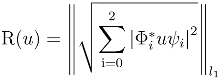
- 3D-TV method.In our paper we also take the 3D TV method in 3D MR image denoising, and the TV norm based on the gradient of the entire volume is specified bywhere Φ0 = Dx; ψ0 = I, Φ1 = Dy; ψ1 = I, and Φ2 = I; ψ2 = Dt; Dx, Dy, Dt are the finite difference matrices along x, y, and t respectively.
2.2. Total Generalized Variation Based Denoising Methods
- (1)
- 2D Second Order TGV method.In order to avoid the staircase effect occurred during image denoising procedure, Bredies et al. proposed a Total Generalized Variation (TGV) method, which can approximate any order polynomial function effectively. And the second order TGV is defined as follows:
 where x is cardiac MR images to be denoised, is the two order TGV penalty function. TGV introduces the auxiliary parameters vand , . In our experiment, we set α0 = 0.02, α1 = 0.06 in this investigation.
- (2)
- 3D Second order TGV method.In this paper, the 3D second order TGV method is proposed to denoise the 3D dynamic MR noisy image. The Total Generalized Variation of second-order is generalized to represent a minimization problem itself [13]:
 Here, we approximate directional derivatives ∇1χ,∇2χ and ∇3χ by D1χ,D2χ and D3χ, where D1, D1 and D3 are the circulant matrixes corresponding to the forward finite difference operators along the x-axis, y-axis and t-axis, respectively, and then ∇χ is approximated by Dχ, ε(p) is approximated by

3. Materials and Methods
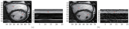
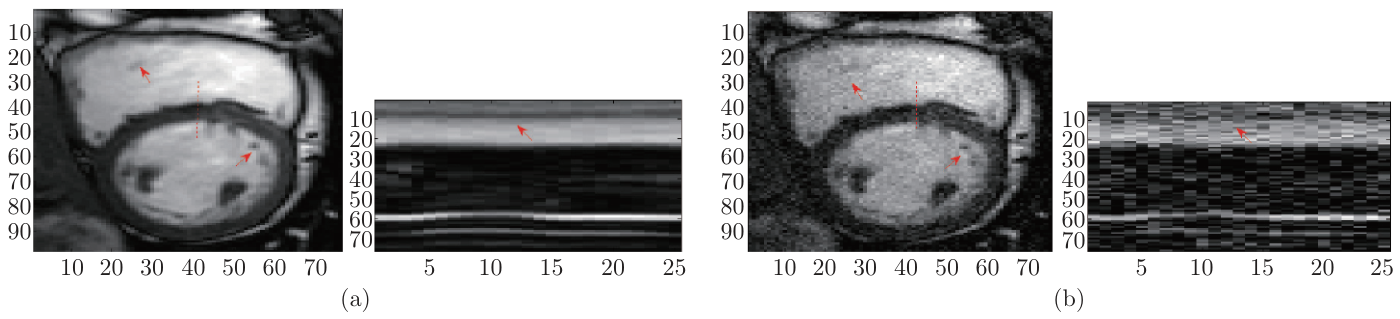
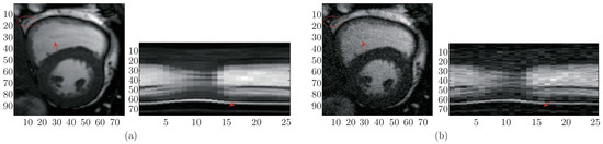
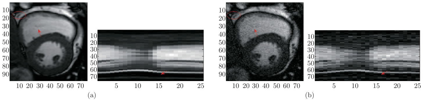
To test the denoising performance of the proposed 3D-TGV method, in vivo cardiac cine MR data was employed in this study, which was acquired on a 1.5T Philips system at Yonsei University Medical Center, and was used in the k-t FOCUSS method [14,15]. The time series data consist of 25 times with an in-plane spatial resolution of 256 × 256. The cine cardiac data was obtained using Steady-state Free Precession (SSFP) sequence with a flip angle of 50 degree and TR=3.45 ms. The FOV was 345 mm × 6270 mm, and the slice thickness was 10 mm. A representative frame and x-t plots of added different kind noise to the cardiac cine MR data are shown in Figure 1 and Figure 2 respectively.
Figure 1.
Dataset: in vivo cardiac cine MR images with Gaussian noise. (a) Left: a representative frame (17th frame), right: the x-t plots of the cine data, and the spatial locations were indicated using dashed lines in (a); (b) Left: a representative frame (17th frame) added with Gaussian noise (with 13.88 B), right: the x-t plots of the noise cine data.
Figure 2.
Dataset: in vivo cardiac cine MR data with random noise. (a) Left: a representative frame (9th frame), right: the x-t plots of the cine data, and the spatial locations were indicated using dashed lines in (a); (b) Left: a representative frame (9th frame) added with random noise (with 14.61 dB), right: the x-t plots of the noise cine data.
All denoising methods were implemented in the Matlab programming environment (Version 2009b, Mathworks, Natick, MA), and the experiments were performed on a ThinkPad laptop with 2.40 GHz Intel Core 2 Duo processor, 4G of memory and Windows 7 operating system. In addition, we compare the proposed 3D-TGV denoising method with another three state-of-the-art dynamic CS-MRI denoising methods, that is, 3D-TV, 2D-TV and 2D-TGV methods.
In this paper, the Signal-to-Noise Ratio (SNR) was employed to quantitatively evaluate the efficiency and accuracy of these denoising methods. Furthermore, the denoised images, their error images (the absolute difference between denoised image and the original MR image), and temporal profile x-t were also compared visually. The SNR was defined as follows:
where MSE was the mean squared error between the denoised MR images (x) and the original image (x0); V ar(x0) denotes the variance of the values in x0.
4. Results and Discussion
In this experiment, in order to test the efficiency and accuracy of these different denoising methods, two different noises, i.e., random noise and Gaussian noise, were considered in this study. In the case of added with two different noises, the denoising performance of 2D-TV, 3D-TV, 2D-TGV and 3D-TGV were analyzed and compared.
4.1. Comparisons on Denoising Gauss Noise
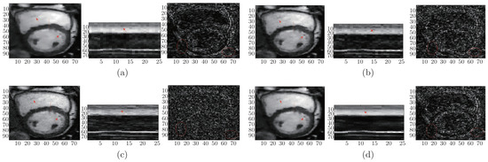
The following is the analysis of the denoising performances on different levels Gaussian noise. The proposed 3D-TGV method was employed to denoise the cardiac MR images. Figure 3, displays the comparisons between 3D-TGV method with 2D-TV, 3D-TV and 2D-TGV denoising methods in denoising the cardiac cine MR dataset when added with Gauss noise (13.87 dB). The denoised MR image of one representative frame (17th frame), the x-t plots of the cine data (the spatial locations were indicated using dashed lines in the reconstructed MR image) and the error map were provided as a comparison. As it can be seen from Figure 3, the proposed 3D-TGV method provided obvious improvement in reducing artefacts, which was presented clearly in the error maps (the third column). And the proposed 3D-TGV method can reconstruct the MR image with clearer border, as shown at the red arrow. The x-t plot of the reconstructions were illustrated in the second column of Figure 3. Each plots displayed the one-dimensional spatial profile, indicated by the dotted line in the first column, at all the temporal frames. It can be found that the proposed 3D-TGV method can capture more details of cardiac dynamics than 2D-TV, 3D-TV and 2D-TGV methods.
Figure 3.
Performance evaluation of 3D-TGV method in comparison with 2D-TGV, 2D-TV and 3DTV methods on the cardiac cine MR dataset which added with Gaussian noise. The first row is the reconstructed MR image with 10.98 dB Gaussian noise; the second row is the x-t plots of the cine data, and the spatial locations were indicated using dashed lines in the first column; the third row is the error map. (a) 2D-TV method; (b) 2D-TGV method; (c) 3D-TV method; (d) 3D-TGV method.
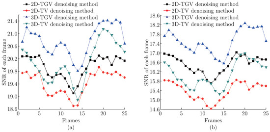
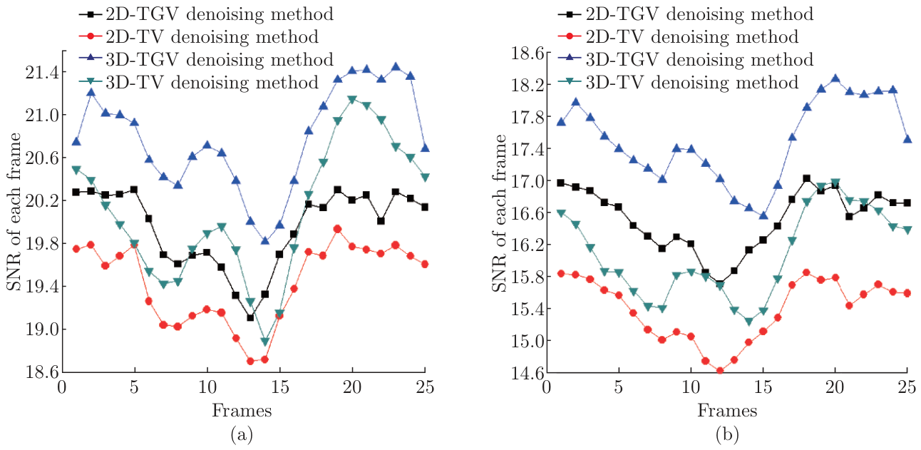
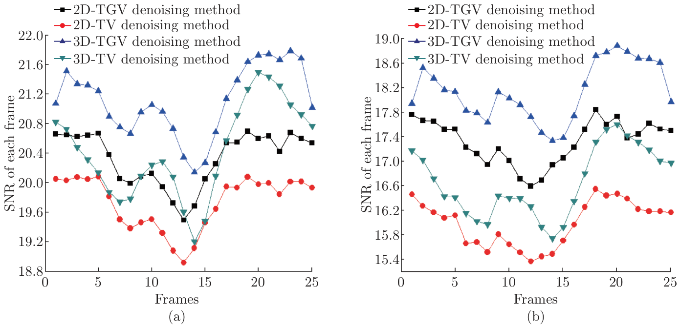
The frame-by-frame SNR of the denoised cardiac MR images presented in Figure 4. As shown in Figure 4, the proposed 3D-TGV denoising method consistently provided higher SNR than 3DTV, 2D-TV, and 2D-TGV methods at all different levels of Gauss noise (16.83 dB, 12.18 dB). Moreover, the 2D-TGV method slightly outperformed not only the 3D-TV with better SNR of most frames but also 2D-TV with better SNR of each frame. On average, the proposed method was superior to the 2D-TGV method by about 1 dB, 3D-TV method by about 1 dB and the 2D-TV method by about 2 dB respectively.
Figure 4.
The SNR of each reconstructed cardiac cine frame with different levels of Gaussian noise by using the 2D-TV, 2D-TGV, 3D-TGV and 3D-TV methods. (a) 16.82 dB; (b) 12.17 dB.
4.2. Comparisons on Denoising Random Noise
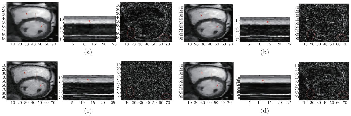
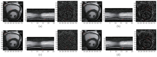
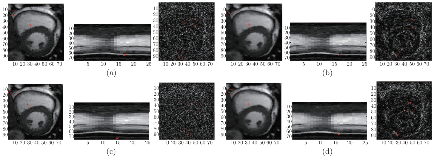
Figure 5 shows the visual comparisons of the denoising results by the using proposed 3D-TGV, 3D-TV, 2D-TV and 2D-TGV methods in denoising random noise (14.610 dB) on the cardiac cine MR dataset. For each sub-figure, the first column was the denoised MR image (9th frame of the cardiac cine data), and the second column showed the x-t plots of the cardiac cine data (the spatial locations were indicated using dashed lines in the reconstructed MR image) and the third column provided the error map. Visually, as shown in Figure 5, one can find that the proposed method outperformed the 2D-TGV, 3D-TV and 2D-TV methods in denoising MR image with better defined borders (as shown in the red arrow in the first column) and less reconstruction artifacts (as shown in the third column). As it can be seen in the second column of Figure 5, the x-t plots of the reconstructions by using the 2D-TGV method and 3D-TV method were contaminated by aliasing artifacts and noises, and the x-t plots of the reconstructions by using 2D-TV method were over-smoothed.
Figure 5.
Denoising Performances of 2D-TV, 2D-TGV, 3D-TV and 3D-TGV methods on the cardiac cine MR images with random noise. The first row is the denoised MR image with 14.61 dB random noise; the second row is the x-t plots of the cine data, and the spatial locations were indicated using dashed lines in the first column; the third row is the error map. (a) 2D-TV method; (b) 2D-TGV method; (c) 3D-TV method; (d) 3D-TGV method.
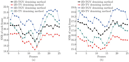
The performance comparisons between the proposed 3D-TGV denoising method and other denoising algorithms, i.e., 2D-TV, 3D-TV and 2D-TGV methods in terms of the SNR frame by frame were also presented in Figure 6. It can be found that the proposed method had the best denoising performances in all these denoising methods, and followed one was the 2D-TGV method, which not only outperformed the 3D-TV methods with higher SNR over most frames but 2D-TV methods with higher SNR over all frames at all reconstruction performance with different levels of random noise (17.12 dB and 12.68 dB). From the denoising accuracy in terms of SNR, it can be seen that the advantages of the proposed 3D-TGV method outperforms its counterpart was apparent. The proposed method can get higher SNR in each frame at different levels with two different noises.
Figure 6.
The SNR of each reconstructed cardiac cine frame with different levels of Random noise by using the 2D-TV, 2D-TGV, 3D-TGV and 3D-TV methods. (a) 17.11 dB; (b) 12.68 dB.
5. Conclusion
In this paper, two different noise, Gauss noise and random noise, were added to the cardiac MR images, which was used to test the denoising efficiency of the proposed 3D-TGV method. Compared with 2D-TV, 3D-TV and 2D-TGV methods in terms of visual comparison and quantitative analysis, the experimental results show that the proposed 3D-TGV method can effectively denoise the two different noises in the cardiac MR images, which can improve the denoising performance obviously with clear border and higher SNR. Moreover, the proposed 3D-TGV method can also be extended to denoising application in video cases.
References
- Rudin, L. I.; Osher, S.; Fatemi, E. Nonlinear total variation based noise removal algorithm. Physica D: Nonlinear Phenomena 1992, Vol. 60(No. 1), 259–268. [Google Scholar] [CrossRef] [Scilit]
- Florian, K.; Kristian, B.; Thomas, P.; Rudolf, S. SFB-Report No. 2010-023; Second Order Total Generalized Variation (TGV) for MRI. 2011.
- Block, K. T.; Uecker, M.; Frahm, J. Suppression of MRI truncation artifacts using total variation constrained data extrapolation. In Proceedings of the 16th Scientific Meeting and Exhibition of ISMRM, Toronto, Canada, 2008. [Google Scholar]
- Hu, Y.; Jacob, M. Higher degree total variation (HDTV) regularization for image recovery. IEEE Transactions on Image Processing 2012, Vol. 21(No. 5), 2559–2571. [Google Scholar] [CrossRef] [Scilit]
- Selesnick, W.; Chen, P. Total variation denoising with overlapping group sparsity. IEEE Int. Conf. Acoust., Speech, Signal Processing (ICASSP), Vancouver, Canada, May 26-31, 2013. [Google Scholar]
- Bredies, K.; Kunisch, K.; Pock, T. Total generalized variation. SIAM Journal on Imaging Sciences 2010, Vol. 3(No. 3), 492–526. [Google Scholar] [CrossRef] [Scilit]
- Cand`es, E. J.; Romberg, J.; Tao, T. Robust uncertainty principles: Exact signal reconstruction from highly incomplete frequency information. IEEE Trans. on Info. Theory 2006, Vol. 52, 489–509. [Google Scholar] [CrossRef] [Scilit]
- saig, T. Y.; Donoho, D. L. Extensions of compressed sensing. Signal Processing 2006, Vol. 86, 533–548. [Google Scholar] [CrossRef] [Scilit]
- Lingala, S. G.; Hue, Y.; DiBella, E.; Jacob, M. Accelerated dynamic MRI exploiting sparsity and low-rank structure: k-t SLR. IEEE Trans. Med. Imaging 2011, Vol. 30(No. 5), 1042–1054. [Google Scholar] [CrossRef] [Scilit]
- Lingala, S. G.; DiBella, E.; Adluru, G.; McGann, C.; Jacob, M. Accelerating free breathing myocardial perfusion MRI using multi coil radial k-t SLR. Phys. Med. Biol. 2013, Vol. 58, 7309–7327. [Google Scholar] [CrossRef] [Scilit]
- Christodoulou, G.; Zhang, H.; Zhao, B.; Hitchens, T. K.; Ho, C.; Liang, Z. High-resolution cardiovascular MRI by integrating parallel imaging with low-rank and sparse modeling. IEEE Trans. Biomed. Eng. 2013, Vol. 60(No. 11), 3083–3092. [Google Scholar] [CrossRef] [Scilit]
- Otazo, R.; Cand`es, E.; Sodickson, D. K. Low-rank plus sparse matrix decomposition for accelerated dynamic MRI with separation of background and dynamic components. Magn. Reson. Med. 2014. [Google Scholar] [CrossRef] [Scilit]
- Knoll, F.; Bredies, K.; Pock, T.; Stollberger, R. Second Order Total Generalized Variation (TGV) for MRI. Magn. Reson. Med. 2011, Vol. 65(No. 2), 480–491. [Google Scholar] [CrossRef] [Scilit]
- Jung, H.; Ye, J. C.; Kim, E. Y. Improved k-t BLAST and k-t SENSE using FOCUSS. Physics in Medicine and Biology 2009, Vol. 52, 3201–3226. [Google Scholar]
- Jung, H.; Sung, K.; Nayak, K. S.; Kim, E. Y.; Ye, J. C. k-t FOCUSS: A general compressed sensing framework for high resolution dynamic MRI. Magnetic Resonance in Medicine 2009, Vol. 61, 103–116. [Google Scholar] [CrossRef] [Scilit]
© 2015 Textile Bioengineering and Informatics Society. This article is an open access article distributed under the terms and conditions of the Creative Commons Attribution (CC BY) license (https://creativecommons.org/licenses/by/4.0/).