AutoML-Based Prediction of Unconfined Compressive Strength of Stabilized Soils: A Multi-Dataset Evaluation on Worldwide Experimental Data

Highlights

What are the main findings?

• The FLAML AutoML framework achieved the most accurate Unconfined Compressive Strength (UCS) predictions (highest average PI score of 0.7848).
• AutoML frameworks demonstrated strong predictive capability for UCS, with performance influenced by dataset size, feature complexity, and optimization strategy.

What are the implications of the main findings?

• The results offer practical guidance for selecting AutoML frameworks based on dataset characteristics, thereby enabling accessible data-driven geotechnical modeling.
• By reducing laboratory workload and experimental time, AutoML frameworks can accelerate data-driven decision-making in the context of soil stabilization projects.

Abstract

Unconfined Compressive Strength (UCS) of stabilized soils is commonly used for evaluating the effectiveness of soil improvement techniques. Achieving target UCS values through conventional trial-and-error approaches requires extensive laboratory experiments, which are time-consuming and resource-intensive. Automated Machine Learning (AutoML) frameworks offer a promising alternative by enabling automated, reproducible, and accessible predictive modeling of UCS values from more readily obtainable index and physical soil and stabilizer properties, reducing the reliance on experimental testing and empirical relationships, and allowing systematic exploration of multiple models and configurations. This study evaluates the predictive performance of five state-of-the-art AutoML frameworks (i.e., AutoGluon, AutoKeras, FLAML, H2O, and TPOT) using analyses of results from 10 experimental datasets comprising 2083 samples from laboratory experiments spanning diverse soil types, stabilizers, and experimental conditions across many countries worldwide. Comparative analyses revealed that FLAML achieved the highest overall performance (average PI score of 0.7848), whereas AutoKeras exhibited lower accuracy on complex datasets; AutoGluon , H2O and TPOT also demonstrated strong predictive capabilities, with performance varying with dataset characteristics. Despite the promising potential of AutoML, prior research has shown that fully automated frameworks have limited applicability to UCS prediction, highlighting a gap in end-to-end pipeline automation. The findings provide practical guidance for selecting AutoML tools based on dataset characteristics and research objectives, and suggest avenues for future studies, including expanding the range of AutoML frameworks and integrating interpretability techniques, such as feature importance analysis, to deepen understanding of soil–stabilizer interactions. Overall, the results indicate that AutoML frameworks can effectively accelerate UCS prediction, reduce laboratory workload, and support data-driven decision-making in geotechnical engineering.

1. Introduction

1.1. Research Background

Unconfined Compressive Strength (UCS) is a measure of the maximum axial load a soil or rock specimen can withstand under compression without any lateral confinement [1]. It is typically determined by applying a steadily increasing axial force to a cylindrical sample until failure occurs [2]. In resource-efficient management of soil-cement materials, accurate and reliable UCS prediction is necessary. Their physical properties primarily influence the UCS of stabilized soils, the design of the stabilization mixture, and the use of appropriate procedures for obtaining the UCS values [3]. Using locally accessible waste materials to replace cement in concrete has also gained attention. In addition, physical, chemical, mechanical, and electrical soil improvements are beneficial [4].

Stabilized natural soils could offer economic and environmental benefits as a sustainable building material. Soil stabilization modifies the physico-mechanical characteristics to satisfy engineering needs. Chemical, dynamical, hydraulic, physical, and mechanical approaches can enhance soil quality as an infrastructure element. Chemical soil stabilization comprises adding lime, cement, silica fume, natural pozzolana, slag, and fly ash to natural soil. Minerals chemically react with soil elements to increase strength and durability. Chemically stabilizing soil reduces the cost of civil engineering applications, such as earth wall construction, foundations, and other earthwork [5]. Among these, Portland cement and lime are standard hydraulic binders used to stabilize soils; however, given their environmental impacts, the continuous manufacturing and use of Portland cement have detrimental effects [6].

Rice husk ash, a byproduct of agricultural activity, has been investigated as a sustainable alternative to cement for soil stabilization [7]. Due to its high silica content, this residue exhibits significant potential as a pozzolanic material, serving either as an additive or as a partial substitute for cement in soil–cement mixtures [4]. However, defining key properties, such as compressive strength, in soils treated with different binder combinations often requires extensive experimental procedures, including trial batching to determine optimal soil–binder ratios, selection of curing periods, and assessment of additional parameters that influence final performance. To address the latter limitations, Machine Learning (ML) approaches have emerged as an alternative for predicting soil compressive strength [8,9]. Despite their potential, the integration of ML into ground improvement assessment has progressed slowly, with documented applications remaining limited: reported studies have employed various algorithms, including Artificial Neural Networks (ANNs), Support Vector Machines (SVMs), regression models, meta-ensemble strategies (voting, stacking, bagging), Functional Networks (FNs), and Multivariate Adaptive Regression Splines (MARSs), to model and predict properties such as strength, dry density, moisture content, additive dosage, and resilient modulus [10,11]. In these works, soil stabilization was carried out using materials such as cement, lime, fly ash, fibers, and geopolymers.

The laboratory approach required substantial effort and resources to obtain reliable conclusions about these variables. Regression analysis was insufficient because researchers used representative mixtures to conduct tests and draw conclusions. Researchers employed ML approaches to analyze their experimental dataset and uncover hidden relationships. Among the evaluated models, Random Forest (RF) stood out for its strong predictive accuracy and generalization capacity. Compared with Support Vector Regression (SVR) and ANN, RF showed greater resistance to noise and outliers while reducing the risk of overfitting. However, its performance was constrained by sensitivity to hyperparameter configurations, motivating the use of optimization algorithms rather than traditional manual tuning methods [12].

Tree-based models have received considerable attention in UCS prediction due to their balance between accuracy and interpretability. Decision trees [13,14,15,16] and random forests [17,18] have been used to model UCS across different soil stabilization contexts. SVM have also been widely employed, taking advantage of their ability to project input variables into higher-dimensional feature spaces and deliver accurate results in several studies [15,19,20,21]. In parallel, genetic programming has been explored as a symbolic regression technique to construct explicit functional relationships between UCS and soil characteristics [22,23,24].

More recent research has highlighted the role of ensemble methods, especially gradient boosting, which combines weak learners into highly predictive models [3,25,26,27]. This technique is particularly useful for handling noisy and nonlinear data [28] and offers a lower computational burden than deep learning. Further improvements have been achieved through metaheuristic optimization of hyperparameters [29,30,31]. Studies also report the use of hybrid approaches, for instance, combining particle swarm optimization (PSO) with gradient boosting [32], adaptive neuro-fuzzy inference systems (ANFIS) [33], and SVM [34]. Other examples include the application of the bat algorithm with SVM to predict UCS of peat-enhanced bricks [35], and the beetle antennae search heuristic for reinforced cemented soils [36].

Beyond UCS prediction, recent studies have demonstrated that integrating machine learning and intelligent optimization can enhance modeling in broader geotechnical contexts. For instance, a multi-source spatio-temporal graph convolutional network (MS-STGCN) was proposed for predicting excavation deformations, effectively capturing spatial–temporal dependencies through deep learning and data fusion [37]. Similarly, a soil parameter back-analysis framework based on the Multi-Level Learning Adaptive Particle Swarm Optimization (MLAPSO) algorithm dynamically updated geotechnical parameters during staged excavations, improving both accuracy and stability [38]. These contributions demonstrate how the same principles that drive hybrid and optimized learning approaches in UCS prediction are now being applied to more complex geomechanical systems, further reinforcing the ongoing shift toward adaptive, data-driven modeling in computational geomechanics.

Furthermore, ANNs remain the most widely used models for UCS prediction, due to their flexibility and ability to represent complex nonlinearities [13,14,39,40]. Das et al. [41] were among the first to employ ANN and SVM for UCS and maximum dry density estimation. Subsequent works extended ANN applications to soils with fibers [42,43,44], road construction [45,46], earthworks decision-making [47], pavement foundations [48,49,50], and sulfate attack resistance in cement-stabilized soils [51]. Alternative formulations, including polynomial neural networks (PNNs) and the group method of data handling (GMDH), were applied to account for UCS nonlinear behavior [52,53,54]. Hybrid ANN–metaheuristic approaches, such as ANN combined with PSO [55,56] or genetic algorithms [57], have also been reported.

The comparative assessments reinforce the strong predictive performance of ANN [58,59,60,61], while tree-based methods and SVM remain competitive alternatives [15,22,62]. Collectively, these data-driven approaches contribute to reducing the reliance on time-consuming laboratory tests and provide robust predictive tools for soil stabilization design.

1.2. Research Motivation

Soil treatment through the addition of stabilizers, such as cement, lime and fly ash, is widely applied to increase soil load-bearing capacity [63,64]. In practice, soil samples are prepared with initial estimates of stabilizer quantities based on normative guidelines, and subsequently tested for UCS [65,66,67]. This process is repeated with different types and proportions of stabilizers until a target UCS value is reached, with each experimental cycle taking 7 to 28 days, in addition to the time required for sample preparation [58].

In recent years, ML models have been increasingly explored to support this process by predicting UCS values based on basic soil parameters and stabilizer properties [10,11]. However, traditional ML approaches still require substantial manual effort in model selection, feature engineering, and hyperparameter tuning, which demands significant expertise and computational resources [68].

Beyond traditional ML, Automated Machine Learning (AutoML) frameworks offer remarkable advantages by automating the entire ML pipeline, including data preparation, feature selection, model selection, parameter fine-tuning, and even Neural Architecture Search [69]. In the considered engineering practice, such automation yields substantial time savings, significantly reducing model development cycles and improving generalization across diverse soil conditions and stabilization methods. Indeed, by systematically exploring a broader configuration space than manual approaches, AutoML frameworks improve model robustness and reproducibility while minimizing human intervention and expertise requirements [70]. The latter strengths make advanced ML modeling accessible to geotechnical practitioners without advanced data science backgrounds, thus accelerating the adoption of data-driven methods in soil stabilization projects [68].

1.3. Research Gap

Relevant keywords were used to identify studies on the application of AutoML for predicting the UCS of soils. The Boolean set (unconfined compressive strength) AND (soil) AND (automated machine learning OR AutoML OR auto machine learning) was applied to the Scopus and Web of Science databases. Only two relevant articles were found; however, in both cases, only the hyperparameter optimization (HPO) step is automated, rather than the entire ML pipeline.

Goliatt et al. [71] employed the Grey Wolf Optimizer (GWO) evolutionary algorithm to support the selection of the most relevant parameters for training a gradient boosting model to predict UCS values. Wang [72] compared three different evolutionary algorithms: the Tunicate Swarm Algorithm (TSA), Sea-horse Optimizer (SHO), and Decision Tree (DT), to optimize feature selection for UCS prediction.

To the best of our knowledge, no approach exists that applies AutoML to UCS prediction throughout the ML workflow data pipeline. Therefore, this study aims to address this gap in the scientific literature.

In contrast, most existing studies that integrate optimization methods with machine learning for UCS prediction have focused exclusively on automating the hyperparameter optimization (HPO) stage. These approaches still rely on manual data preprocessing, feature selection, and model choice, which restricts their scalability and reproducibility. The proposed end-to-end AutoML workflow presented in this study extends automation to all major stages of the machine learning pipeline, encompassing data preprocessing, feature selection, model selection, and hyperparameter tuning. This comprehensive automation minimizes human bias, reduces the dependency on expert knowledge, and enhances reproducibility across studies. Table 1 summarizes a comparison between representative works that employ traditional ML combined with metaheuristic optimization methods and the present fully automated AutoML workflow.

Table 1. Comparison of automation levels across the main stages of the ML workflow between previous UCS prediction studies and the present fully automated AutoML framework.

Study	Data Preprocessing	Feature Selection	Model Selection	Hyperparameter Tuning	Evaluation	Workflow Type
Ngo et al. (2023) [73]	Manual normalization	Manual correlation check	SVM-based model predefined	Meta-heuristic (PSO/GA)	Manual with regression metrics	Semi-automated
Kardani et al. (2021) [57]	Manual preprocessing	Not applied	Predefined regression models	Evolutionary algorithm	Manual performance analysis	Semi-automated
Onyelowe et al. (2024) [74]	Standardized inputs	Statistical filtering (RFE)	Ensemble model comparison	Grid/Random search	Manual cross-validation	Semi-automated
Teodoru et al. (2025) [75]	Automated scaling and cleaning	Recursive feature elimination	Model comparison via Auto-sklearn	Bayesian optimization (Optuna)	Automated	Partially automated
Yao et al. (2024) [76]	Manual preprocessing	Importance ranking via SHAP	Hybrid XGB architecture	Hybrid optimization (XGB-based)	Manual evaluation	Semi-automated
This paper	Fully automated preprocessing (encoding, scaling, imputation)	Automated feature selection (embedded and filter-based)	Automated model search (multiple AutoML frameworks)	Automated tuning (Bayesian + meta-heuristics)	Automated performance evaluation and reporting	End-to-end AutoML

The table contrasts prior UCS prediction studies using traditional machine learning with manual or semi-automated workflows against the present work, which achieves full automation from preprocessing to evaluation.

1.4. Objectives and Significance of the Study

The present study aims to address the limitations of conventional trial-and-error approaches in soil stabilization by using AutoML frameworks to predict UCS values from simple soil parameters. The study evaluates and compares five state-of-the-art frameworks currently available in the literature and software market. The goal is to assess their predictive capacity for UCS and their suitability for geotechnical engineering applications.

A central objective is to employ these AutoML frameworks on ten independent experimental datasets collected from multiple countries worldwide, considering each dataset as a separate modeling scenario. Such a multi-dataset evaluation is designed to assess how consistently different AutoML frameworks perform across heterogeneous soil–stabilizer conditions, rather than to construct a single unified global model. By benchmarking performance across these independent datasets, the study provides insight into the robustness and transferability of AutoML-based UCS prediction under diverse geotechnical settings.

The significance of the developed research is threefold. First, it demonstrates that AutoML can substantially reduce development time and resource requirements while maintaining predictive accuracy, thereby offering practical time and cost savings for the considered engineering applications. Second, by incorporating datasets from different regions and soil conditions, the current study evaluates explicitly the generalization capability of AutoML frameworks across multiple different real-world scenarios, hence addressing the critical need for robust and transferable predictive models in geotechnical practice. Third, the conducted comparative analysis provides practical guidance for selecting appropriate AutoML tools based on specific project requirements, dataset characteristics, and computational constraints.

The remainder of the manuscript is structured as follows: Section 2 presents the dataset and describes the computational ensemble framework. Section 3 reports the computational experiments and discussion. The final remarks and conclusion are provided in Section 4.

2. Material and Methods

2.1. Datasets Description

Table 2 presents a summary of the ten experimental datasets consisting of 2083 samples acquired from laboratory experiments encompassing diverse soil/rock types, stabilizers, input predictor variables used for model training, and experimental conditions from many countries worldwide. Most soils were classified according to the USCS (Unified Soil Classification System) [77], and the names of the corresponding symbols can be found in Table 3.

Table 2. Dataset summary.

Dataset and Reference	No. Samples	No. Variables	Soil/Rock Type *	Stabilizer	Country
D1 [58]	179	7	Various 1	Lime	USA
D2 [58]	60	7	Various 2	Cement	USA
D3 [78]	216	14	Various 3	Cement	Vietnam
D4 [79]	129	5	CL	Various 4	India 5
D5 [80]	283	8	CH and CL	Geopolymer	India
D6 [81]	408	9	Various 6	Various 7	Various 8
D7 [82]	137	6	SM and MH	CLR 9	Malaysia
D8 [83]	170	4	Various 10	– 11	Iran
D9 [84]	351	7	Sands	MICP 12	Various 13
D10 [12]	150	3	CH	Various 14	China

* Soils classified according to USCS are marked with symbols, in these cases, refer to Table 3; ¹ CH, OL, CL, ML, OH, SC, SM, GC and GM; ² SP-SM, CH, SM, ML, CL, GC, GM and SC; ³ yellow clay, black organic sandy clay and black sandy clay; ⁴ pond ash, rice husk ash and cement; ⁵ given that India has many deposits of kaolin clay, a mineral widely extracted in the country, and that the authors are affiliated with Indian institutions, it is reasonable to infer that the experiments and sample collection were likely carried out in India; ⁶ CL, ML, MH, CH and CL-ML; ⁷ lime, cement, pozzolanic materials and fly ash; ⁸ Algeria, USA, Türkiye, India, Bangladesh and Australia; ⁹ various combinations of cement, lime, and rice husk ash (CLR) mixtures; ¹⁰ claystone, granite, schist, sandstone, travertine, limestone, slate, dolomite and marl; ¹¹ there is no stabilizer because the study conducts tests with rocks; ¹² microbially induced calcite precipitation (MICP); ¹³ Germany, Australia, USA and China; ¹⁴ cement and glass fiber reinforced polymer (GFRP).

Table 3. Soil classification according to the Unified Soil Classification System (USCS).

Group Symbol	Group Name
GW	Well-graded gravels
GP	Poorly graded gravels
GM	Silty gravels
GC	Clayey gravels
SW	Well-graded sands
SP	Poorly graded sands
SM	Silty sands
SC	Clayey sands
ML	Low-plasticity silts
CL	Low-plasticity clays
OL	Organic soils with low compressibility
MH	High-plasticity silts
CH	High-plasticity clays
OH	Organic soils with high compressibility
PT	Highly organic soils (Peat)

Table A1, Table A2, Table A3, Table A4, Table A5, Table A6, Table A7, Table A8, Table A9 and Table A10 in Appendix A show the descriptive statistics information for all used datasets. From the tables in Appendix A, one can see that the mean UCS (MPa) values range from 0.258 (dataset D4 for stabilized Kaolin clay) to 96.0 (dataset 8 for stabilized different rock types).

Figure 1 illustrates the geographical distribution of the samples included in the datasets. The color intensity reflects the relative frequency of samples per country, with red darker shades indicating a higher number of samples and red lighter shades representing lower sample counts.

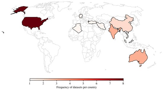
Figure 1. Geographical distribution of dataset sample locations.

One of the objectives of Gajurel et al. [58] was to consolidate seven publicly available source datasets for training and testing ML algorithms that predict the UCS of soils stabilized with lime (dataset D1) and cement (dataset D2). The input variables used for model training included the Atterberg limits (i.e., liquid limit, plasticity index), particle-size distribution (i.e., silt content, sand content), organic content, stabilizer properties, and dosage. Soil samples were collected from various regions across the United States, including Iowa, Florida, Illinois, Texas, Michigan, Virginia, North Carolina, and Tennessee.

The D3 dataset used the source data by Ngo et al. [78], comprising 14 input parameters, to train an ML algorithm to predict the UCS of cement-soil mixtures. Samples were collected in Hai Duong city, Vietnam. These parameters are categorized as follows:

• Soil and mix composition characteristics: soil type (S), moisture content (Mc), wet density (We), sampling depth (D), and amount of cement (Ac).
• Specimen geometry and physical properties after mixing: specimen diameter (Di), specimen length (L), specimen area (A), specimen volume (V), specimen mass (M), and specimen density (De).
• Curing conditions: curing condition (Cc), curing period (Cp, expressed in days), and type of cement (T).

The D4 dataset with experimental results presented by Priyadarshee et al. [79] on Kaolin clay considered the following input parameters: clay content (C), pond ash content (PC), rice husk ash content (RC), cement content (CC), and curing period (CP). These variables were used as predictors in the model development process, while the UCS of the soil specimens served as the output variable. The article does not specify the exact location where the experimental data were collected, reporting only that the material studied was kaolin clay.

The D5 dataset comes from the study by Mozumder and Laskar [80], which selected ground granulated blast furnace slag (GGBS), fly ash (FA), and a blend of GGBS and FA (GGBS + FA) as source materials for geopolymerization. The model used the following input parameters: Atterberg limit (i.e., liquid limit, plasticity index), percentage of GGBS (%S), percentage of FA (%FA), molar concentration (M), alkali-to-binder ratio (A/B), sodium-to-aluminum ratio (Na/Al), and silicon-to-aluminum ratio (Si/Al). The output parameter was the 28-day UCS of the soil, expressed in MPa, and samples were collected from India (Silchar city).

The D6 dataset, containing experimental data by Taffese and Abegaz [81], aimed to predict the UCS of soils by consolidating seven publicly available datasets for training and testing ML algorithms. The model employed input features describing the mix ratios and categories of stabilized soils, plasticity characteristics (Atterberg limits), soil classification indices, and compaction parameters such as optimum moisture content (OMC) and maximum dry unit weight (MDD). The dataset encompasses a diverse range of soils collected from twelve countries across Africa (Chlef town, Algeria), the Americas (Oklahoma, USA), the Middle East (Trabzon city, Türkiye), South Asia (India and Bangladesh), and Oceania (Queensland and New South Wales, both in Australia). The soils were stabilized using various techniques, including lime, cement, pozzolanic materials, and fly ash.

The D7 dataset was developed based on Tabarsa et al. [82], which predicted UCS for silty sand and high-plasticity silt in Malaysia stabilized with various combinations of cement, lime, and rice husk ash (CLR) mixtures. The input variables used for model training included: soil type, dry unit weight (${\gamma }_d$), curing time, cement content (C), lime content (L), and rice husk ash content (R).

The main objective of the study by Mahmoodzadeh et al. [83] was to use the D8 dataset to predict the UCS of different rock types of Claystone (Cl), Granite (Gr), Schist (Sc) and Sandstone (Sa), Travertine (Tr), Limestone (Li), Slate (Sl), Dolomite (Do) and Marl (Ma), located at Iran. The prediction models employed variables such as porosity (n), Schmidt hammer rebound value (SH), P-wave velocity ($V_p$), and point load index ($I_{s\left(50\right)}$) as input parameters.

The study by Wang and Yin [84] compiled thirteen datasets available in the scientific literature (dataset D9) to predict the UCS of soils treated biochemically using the microbially induced calcite precipitation (MICP). The technique relies on introducing urease-producing bacteria together with a cementing solution. Seven variables were used to train the model: average particle diameter, gradation coefficient, starting void ratio, turbidity of the bacterial solution, urea concentration, calcium ion content, and amount of calcium carbonate formed. The samples were collected in various regions, including Germany, Australia, the USA (Ottawa, Mississippi, and Nevada), and China [85,86,87,88,89,90,91,92,93,94,95,96].

One of the objectives of Zhang et al. [12] study was to use dataset D10 to predict the UCS of soils treated with cement and glass fiber reinforced polymer (GFRP). The model was trained using the following variables: cement proportion, water content, and curing period. Soil samples were collected from China.

2.2. Cross-Validation (CV)

Cross-Validation (CV) assesses the predictive ability of models and reduces errors caused by overfitting. One technique used was k-fold cross-validation, which divides the dataset into k folds of similar size. In each iteration, the model is fitted on the $k-1$ training folds and evaluated on the test fold. The procedure is repeated k times, so that each fold serves as validation once [97]. Figure 2 demonstrates the k-fold CV with five folds, in which, in each round, one of the folds is designated as the test set (in blue), while the other four form the training set (in gray). The value of k used in this study was equal to 5.

Figure 2. Example of a k-fold CV with 5 folds.

2.3. Automated Machine Learning (AutoML)

AutoML is an automated methodology that enables the construction of ML models to streamline and accelerate tasks that consume significant time in data modeling [69,98]. It aims to reduce model training time and improve predictive performance, enabling users with varying levels of ML experience to build high-quality models more efficiently and at lower computational cost [99,100].

In recent years, AutoML techniques have gained prominence and demonstrated considerable influence across multiple sectors. Within finance, they have been applied to tasks such as fraud detection, credit scoring, and risk evaluation by automating the identification of the most suitable ML models [101]. In healthcare, applications include disease prediction based on genetic profiles, patient medical history and physiological signals [102,103]. The manufacturing industry has benefited from AutoML by leveraging it to anticipate equipment malfunctions and enhance production efficiency [104]. In the retail domain, these tools are employed for demand forecasting and to support logistics optimization [105,106]. Environmental and energy-related applications are also gaining momentum: AutoML has been successfully employed for streamflow forecasting, supporting water-resource planning and hydropower management [107], and for predicting bio-oil yield from lignocellulosic biomass pyrolysis, where it has proven effective in optimizing renewable energy production processes [108]. Lastly, more recently, AutoML frameworks have been evaluated in the construction sector, where they have been applied to predict the compressive and flexural strength of recycled aggregate concrete, contributing to sustainable construction practices and promoting circular economy principles [109].

A comparative overview of the five AutoML frameworks examined in the developed study is presented in Table 4. At the same time, the following sections provide a more detailed discussion of their performance attributes and functional capabilities. It is worth noticing that the exploited AutoML frameworks were selected based on the following criteria: (1) they are open source and freely available, thus ensuring full reproducibility; (2) they represent different optimization strategies; (3) they are well-established in the AutoML literature with active developer communities [100]; and (4) they support tabular data regression tasks, which aligns with the faced UCS prediction problem. Last, but not least, we excluded proprietary or cloud-based frameworks to ensure consistent and fully reproducible evaluation conditions without relying on external commercial services or incurring additional costs.

Table 4. Overview of Evaluated AutoML Frameworks.

Framework	Release Date	Optimization Technique	ML Toolbox	Meta-Learning	Post-Processing
AutoKeras [110,111]	2019	Bayesian Optimization	Keras, TensorFlow	No	Yes
AutoGluon [112]	2020	Ensemble-Based Search	MXNet, PyTorch 2.4.0	Yes	Yes
FLAML  [113]	2021	Cost-Aware Search	flaml	No	No
H2O [114]	2020	Random and Ensemble-Based	h2o	Yes	Yes
TPOT  [115]	2016	Genetic Programming	scikit-learn	No	Yes

2.3.1. Auto-Keras

Auto-Keras is an open-source AutoML framework developed by the Texas A&M University DATA Lab for automating the process of building and optimizing ML models [111]. One advantage of using Auto-Keras is that it does not require Docker or Kubernetes in the cloud. Unlike other AutoML models, Auto-Keras uses deep learning algorithms. The use of AutoKeras is mainly justified by three points: (i) AutoKeras is entirely free, in contrast to many cloud-based AutoML solutions that require subscriptions or pay-per-use; (ii) its interface was made to be usable by people without advanced computer science training, in contrast to many cloud services that demand specialized knowledge; and (iii) AutoKeras can be run locally on personal computers, ensuring broad availability and removing privacy and data security concerns that are frequently linked to the use of external platforms [111].

Figure 3 shows the AutoKeras architecture, which optimizes CPU, GPU, and memory usage by keeping only active data in RAM. To perform specific tasks, the user-driven API communicates with intermediate modules. Using Gaussian processes and CPU-based optimizers, Bayesian optimization guides the architecture search.

Figure 3. Auto-Keras schematic framework.

2.3.2. AutoGluon

AutoGluon-Tabular is a Python-based framework designed for AutoML on tabular data and is recognized for its high accuracy [112]. The tool utilizes multi-layered ensemble techniques, deep learning methods, and advanced data processing approaches. Furthermore, it enables the automatic identification of data types in each column, allowing for safe preprocessing that manipulates textual fields differently. To enable the transformation of raw data into high-quality predictions within a given timeframe, under constraints, AutoGluon fine-tunes multiple models arranged in multiple layers, which are trained sequentially, as shown in Figure 4.

Figure 4. AutoGluon schematic framework.

2.3.3. Fast Lightweight AutoML (FLAML)

Fast Lightweight AutoML (FLAML) is a Python-based library that delivers efficient AutoML with minimal computational cost [113]. Instead of relying on exhaustive exploration, it structures the search space to prioritize configurations that optimize both predictive accuracy and runtime cost. Throughout this process, the framework adaptively determines the learning algorithm, hyperparameter values, data subsampling size, and resampling strategy, considering their joint influence on performance and resource consumption. An overview of its architecture is illustrated in Figure 5.

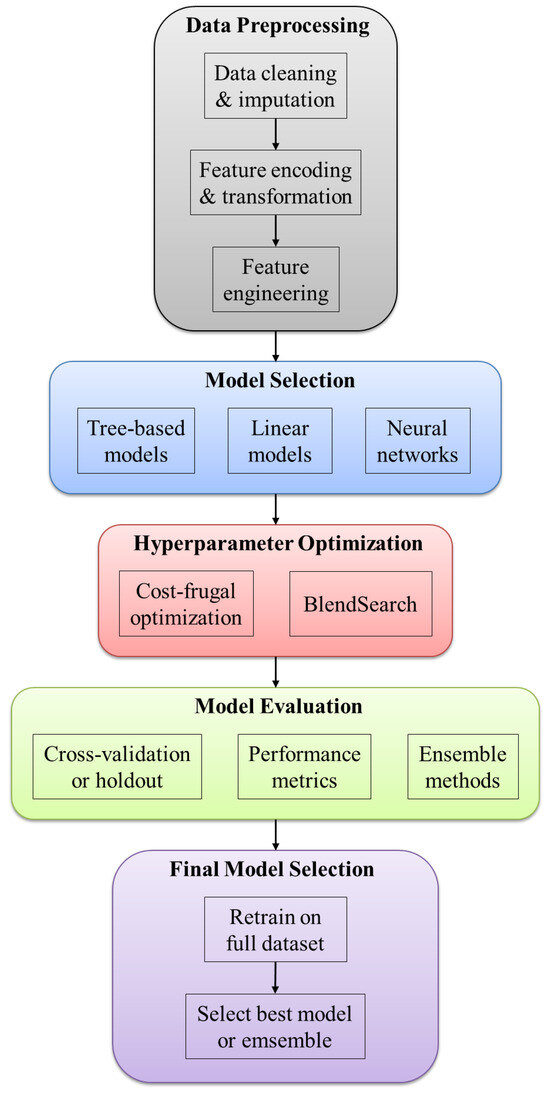
Figure 5. FLAML schematic framework.

2.3.4. H2O

H2O AutoML is a feature of the H2O framework that automates ML tasks and generates reliable, enterprise-ready models with ease of use. For tabular data, it facilitates supervised training on regression, binary, and multiclass classification problems [114]. H2O AutoML performs the same automatic preprocessing as available in H2O’s supervised algorithms, including one-hot encoding for XGBoost models, normalization when required, and imputation of missing values. Grouping categorical variables is enabled by tree-based models, such as Random Forests and Gradient Boosting Machines, which process categorical data directly. The H2O AutoML interface is designed to be intuitive, requiring only the user to provide the dataset and the variable of interest. Additionally, it is possible to optionally specify a maximum runtime or a maximum number of models to create [114]. Figure 6 provides an overview of the framework.

Figure 6. H2O schematic framework.

2.3.5. Tree-Based Pipeline Optimization Tool (TPOT)

The TPOT framework, represented in Figure 7, employs Genetic Programming (GP) to automatically create and optimize ML pipelines [115]. At the beginning of each run, TPOT generates an initial set of pipelines that form the Genetic Programming population. This population is then iteratively refined using selection mechanisms that favor pipelines with the highest predictive performance. The evolutionary process continues until the user-defined number of iterations is reached or the established convergence criteria are met. At the end of this optimization process, the pipeline with the best predictive performance is selected and retained as the final solution.

Figure 7. TPOT schematic framework.

2.3.6. Imputation Strategies Across AutoML Frameworks

Heterogeneous strategies for handling missing values are implemented by the AutoML frameworks assessed in this study, which can affect model behavior, especially in small datasets. We outline the imputation techniques used by each framework in its default setup to ensure methodological transparency.

AutoGluon assigns the underlying learners to handle missing values. By using natural split-based handling, tree-based estimators (LightGBM, CatBoost, XGBoost) avoid explicit imputation. AutoGluon uses basic univariate imputation, typically the mean (numerical) or the most frequent value (categorical), for models that do not accept missing values. As a result, imputation is hybrid and model-dependent, fusing native methods with backup plans.

For model training to succeed, AutoKeras requires complete data and does not perform automatic imputation. AutoKeras did not perform any imputation because the datasets used in this investigation had no missing values after integration.

FLAML provides missing values straight to the chosen estimators without using explicit imputation. While learners without this functionality require the whole dataset, tree-based learners naturally handle missing values. In this investigation, no imputation was used.

Algorithm-specific preprocessing is used by H2O. Mean imputation is applied to numerical features in non-tree models, whereas a unique “missing” category is assigned to categorical characteristics. Without imputation, tree-based algorithms use natural split mechanisms to handle missing data. The final plan is a hybrid imputation method that is automatically activated during model training.

TPOT uses scikit-learn operators to evolve pipelines. TPOT adds a SimpleImputer phase when there are missing values, typically using the mean (numerical) or the most frequent value (categorical) imputation. Because of the absence of missing data, this operator was not applied in this study, even though it was present in the search space.

2.3.7. AutoML Framework Parameters

The definition of hyperparameters is a critical step to guarantee the reproducibility, comparability, and fairness of experiments involving different AutoML frameworks. In this study, the configuration of each framework was established according to its official documentation and adapted to the computational budget and dataset characteristics.

Other parameters were selected to reflect standard practices reported in the literature, while maintaining a consistent setup across the evaluated methods. This approach ensures that the evaluation focuses on the relative modeling capacity and search strategies of each framework, rather than differences in configuration. Table 5 summarizes the complete set of hyperparameters used for each AutoML framework in this work.

Table 5. Hyperparameters defined for each AutoML framework. The time budget for FLAML and H2O was chosen based on preliminary testing, which indicated that 120 s (the overall limit for each run) was sufficient to find optimal or near-optimal results for the models, balancing the goal of achieving the best predictive performance with the requirement for computational efficiency and accelerated development time.

Framework	Parameter	Value
AutoGluon	label	target
	verbosity	False
	time_limit	120 s
AutoKeras	max_trials	50
	epochs	100
	column_names	feature_names
	loss	mean_absolute_error
FLAML	time_budget	120 s
	metric	MAE
	task	regression
	estimator_list	[lgbm, rf, xgboost, extra_tree, xgb_limitdepth, catboost, kneighbor]
	verbose	False
	n_jobs	2
H2O	nthreads	2
	max_runtime_secs	120 s
	sort_metric	RMSE
TPOT	max_time_mins	2 (120 s)
	generations	20
	population_size	20
	cv	5
	verbosity	False
	n_jobs	2

The parameters presented in Table 5 were kept fixed throughout the experiments, ensuring that comparisons across frameworks were conducted under consistent computational constraints.

2.4. Model Development and Validation Procedures

The model development process was conducted by applying four distinct AutoML frameworks: AutoGluon, H2O, FLAML, and TPOT. Each framework was trained and validated using a stratified split of the considered dataset, with 70% allocated for training and internal cross-validation and 30% reserved for testing. Data preprocessing tasks, including normalization, handling categorical variables, and outlier detection, were handled natively by each framework. To mimic realistic application scenarios, both the default parameters and the recommended settings from the tools were used. Given the substantial differences in materials, laboratory procedures, available predictors, and sample sizes across the employed datasets D1–D10 (refer to Section 2.1), all AutoML models were trained and evaluated separately on each dataset. No single model was fitted jointly to the combined data; instead, model performance was compared across datasets. All experiments were conducted in the same computational environment, comprising hardware and software, to ensure fair comparability. Model performance was assessed through the k-fold CV technique (reported in Section 2.2) integrated with AutoML frameworks, and the final results represent averages over 30 independent repetitions to ensure statistical reliability.

2.5. Performance Metrics

The assessment focused on standard regression metrics, including the Mean Absolute Error (MAE), Mean Absolute Percentage Error (MAPE), Root Mean Square Error (RMSE), Pearson Correlation Coefficient (R), and the Coefficient of Determination (R²) (Table 6). The latter metrics were selected to provide a comprehensive assessment of model performance from multiple perspectives: MAE and RMSE capture the magnitude of prediction errors, with MAE providing a linear measure of average error and RMSE being more sensitive to large errors due to its quadratic nature. MAPE expresses the error as a percentage, thereby offering an intuitive understanding of relative error; however, it can be less stable when actual values are near zero; for this reason, we also report the Symmetric Mean Absolute Percentage Error (SMAPE) so that the results of both metrics can be compared consistently. R measures the strength of the linear relationship, and R² quantifies the proportion of variance explained by the model. Together, the selected metrics allow for a balanced evaluation of both the absolute and relative accuracy of the predictions, as well as the model’s overall fit.

Table 6. Acronyms and expression for the performance metrics.

Metric Acronym	Expression
MAE	${\displaystyle \frac{1}{N}\sum _{t=1}^N\left|(y_i-{\widehat{y}}_i)\right|}$
MAPE	${\displaystyle {\displaystyle \frac{1}{N}}\sum _{i=1}^N\left|\frac{y_i-{\widehat{y}}_i}{y_i}\right|\times 100\%}$
RMSE	${\displaystyle {\displaystyle \frac{1}{N}}\sqrt{\sum _{i=1}^N{(y_i-{\widehat{y}}_i)}^2}}$
R	${\displaystyle \frac{cov(y,\widehat{y})}{\sqrt{var\left(y\right)}\sqrt{var\left(\widehat{y}\right)}}}$
R2	${\displaystyle \sum _{i=1}^N{\displaystyle \frac{{(y_i-{\widehat{y}}_i)}^2}{{(y_i-\overline{y})}^2}}}$
SMAPE	${\displaystyle {\displaystyle \frac{1}{N}}\sum _{i=1}^N\frac{2\times |y_i-{\widehat{y}}_i|}{\left|y\right|+|\widehat{y}|}\times 100\%}$

Although R and R² are mathematically related, they provide different perspectives on model behavior. R measures the strength of the linear association between predicted and observed values, while R² quantifies the proportion of variance explained by the model. The decision to report multiple metrics aligns with the general principle discussed by Nguyen et al. [116], who highlight that no single metric is sufficient to characterize predictive performance. Their study evaluates models using several error-based metrics, each capturing a different facet of model behavior, such as absolute error magnitude, sensitivity to outliers and relative deviation. Following the same rationale, we report both R and R² to provide complementary insights into linear agreement and explanatory capacity. R quantifies the strength and direction of the linear association between predictions and actual values and is particularly useful for interpreting scatter plots and assessing whether the model preserves monotonic tendencies. R² quantifies the proportion of variance explained and is particularly relevant when evaluating models on datasets with pronounced variability across samples. The combined use of these metrics therefore provides a broader and more transparent characterization of predictive behavior.

2.6. Feature Importance

Determining which features most significantly affect model predictions is crucial for evaluating the reliability and interpretability of ML frameworks. Feature importance analysis clarifies whether algorithms prioritize variables with significant physical or geotechnical meaning, thereby enhancing the understanding of predictive results. In this study, we assessed feature importance by combining feature-target correlations with permutation importance scores, providing a comprehensive view of how each AutoML framework prioritizes input variables. The following discussion highlights consistent trends across datasets and notes instances in which feature selection deviated from expected patterns, thereby affecting model performance.

To evaluate the role of each input variable in model predictions, we applied the permutation feature importance method [117]. This approach estimates importance by measuring the increase in prediction error when the values of a given variable are randomly shuffled, which disrupts its association with the target. For each variable, a baseline performance score was computed on the original test set using mean squared error as the metric. The variable values were then permuted 100 times, and the resulting performance changes were averaged to obtain the importance score. Larger average differences indicated greater importance [118].

The procedure was applied across all AutoML frameworks, with specific adjustments made for AutoGluon and H2O to accommodate their respective data input requirements. The results of this analysis offered key insights into the variables most influential to model performance, while also supporting the interpretation of predictive accuracy across datasets.

3. Computational Experiments

3.1. Computational Settings

The computational experiments were carried out in Python. The computer specifications are as follows: Intel(R) Core(TM) i7-9700F (8 cores at 3 GHz, 6 MB cache), 32 GB RAM, and Ubuntu Linux 22. Table 7 shows the libraries used and their respective versions.

Table 7. Python (3.9.23 Version) libraries and versions used. The dataset was divided into 70% for training and 30% for testing in each run (30 runs in total). At each iteration ($run$), a different random seed was used ($seed=run\times 37+1001$) to obtain different splits in the k-fold cross-validation, with $k=5$ in the training set. Each run uses a deterministic seed.

Library	Version
AutoGluon	0.7.0
AutoKeras	1.0.20
Cython	3.1.3
FLAML	1.2.4
H2O	3.44.0.3
Jinja2	3.1.6
Joblib	1.5.1
Keras-Tuner	1.4.7
Matplotlib	3.9.4
NumPy	1.23.5
Openpyxl	3.1.2
Pandas	1.5.3
Permetrics	2.0.0
Scikit-Learn	1.2.2
Scipy	1.11.4
Seaborn	0.12.2
Skillmetrics	1.1.8
TPOT	0.12.1
Tensorflow	2.9.3

3.2. Comparison of AutoML Frameworks

Figure 8 presents the mean execution time in seconds for each dataset and framework. AutoGluon and AutoKeras achieved the shortest execution times, followed by FLAML and H2O, whereas TPOT produced the longest execution time. It is important to note that no time limit was applied to AutoGluon or TPOT, and AutoKeras does not provide a parameter to restrict execution time. For FLAML and H2O, a limit of 120 s was used, which explains the values shown in Figure 8.

Figure 8. Average runtime in seconds runs for each dataset and framework.

Table 8 reports the mean values and standard deviations for each dataset, including the performance metrics obtained by all AutoML frameworks. The results reported in the original studies from which each dataset was derived are also provided, denoted as “Ref.”, and correspond to the best performance obtained by each evaluated model (Table 9 lists these models). An exception is the study by Wang and Yin [84], where the reported values represent the average across groups rather than the best single result. As Goliatt et al. [71] conducted experiments on datasets D1 to D6, their results were also reported for comparison.

Table 8. Averaged performance metrics with standard deviations in parentheses. Entries indicated with (-) indicate that the value is not available. Entries in boldface highlighted the best results.

Dataset	Model/Framework	R	R2	RMSE	MAE	MAPE (%)	SMAPE (%)
D1	AutoGluon	0.904 (0.037)	0.819 (0.066)	0.234 (0.055) MPa	0.163 (0.034) MPa	128.371 (139.790)	47.462 (6.699)
	AutoKeras	0.902 (0.042)	0.816 (0.073)	0.234 (0.048) MPa	0.152 (0.027) MPa	92.089 (109.954)	47.301 (7.186)
	FLAML	0.912 (0.056)	0.835 (0.098)	0.217 (0.063) MPa	0.146 (0.031) MPa	137.759 (177.942)	47.485 (6.680)
	H2O	0.928 (0.031)	0.863 (0.057)	0.202 (0.043) MPa	0.140 (0.026) MPa	94.955 (110.567)	45.990 (6.242)
	TPOT	0.894 (0.043)	0.801 (0.076)	0.243 (0.050) MPa	0.169 (0.030) MPa	149.595 (186.377)	48.707 (7.180)
Ref. [58]	SVR	-	0.75	0.50 MPa	0.44 MPa	-	-
Goliatt et al. [71]	XGB	0.964	0.928	0.148 MPa	0.101 MPa	-	-
D2	AutoGluon	0.752 (0.161)	0.525 (0.323)	0.875 (0.257) MPa	0.617 (0.201) MPa	42.235 (14.832)	60.526 (14.097)
	AutoKeras	0.867 (0.146)	0.744 (0.261)	0.584 (0.184) MPa	0.403 (0.120) MPa	32.049 (13.506)	55.515 (13.795)
	FLAML	0.778 (0.152)	0.579 (0.276)	0.820 (0.203) MPa	0.582 (0.158) MPa	40.229 (14.214)	61.195 (12.662)
	H2O	0.713 (0.259)	0.462 (0.471)	0.895 (0.407) MPa	0.674 (0.344) MPa	43.297 (18.931)	62.467 (16.609)
	TPOT	0.815 (0.180)	0.696 (0.242)	0.676 (0.188) MPa	0.489 (0.126) MPa	35.099 (12.928)	56.329 (14.001)
Ref. [58]	MLR	-	0.82	0.53 MPa	0.45 MPa	-	-
Goliatt et al. [71]	XGB	0.910	0.826	0.596 MPa	0.390 MPa	-	-
D3	AutoGluon	0.901 (0.051)	0.814 (0.086)	0.489 (0.115) MPa	0.376 (0.084) MPa	25.594 (7.692)	22.026 (4.751)
	AutoKeras	0.889 (0.057)	0.763 (0.192)	0.538 (0.191) MPa	0.375 (0.101) MPa	21.883 (4.757)	20.949 (4.266)
	FLAML	0.908 (0.030)	0.825 (0.054)	0.475 (0.066) MPa	0.367 (0.047) MPa	24.596 (4.581)	22.403 (3.178)
	H2O	0.915 (0.038)	0.839 (0.067)	0.452 (0.063) MPa	0.347 (0.048) MPa	23.585 (4.219)	21.632 (3.908)
	TPOT	0.898 (0.064)	0.810 (0.106)	0.484 (0.122) MPa	0.366 (0.073) MPa	24.747 (5.713)	22.424 (4.400)
Ref. [78]	ANN	0.925	-	0.419 MPa	0.292 MPa	-	-
Goliatt et al. [71]	XGB	0.940	0.882	0.410 MPa	0.312 MPa	-	-
D4	AutoGluon	0.967 (0.018)	0.936 (0.034)	19.316 (6.020) kPa	14.137 (3.778) kPa	5.747 (1.565)	5.622 (1.467)
	AutoKeras	0.685 (0.176)	0.456 (0.259)	55.800 (12.711) kPa	43.646 (10.590) kPa	17.903 (4.246)	17.540 (4.231)
	FLAML	0.980 (0.014)	0.961 (0.028)	14.758 (5.116) kPa	11.042 (3.477) kPa	4.597 (1.613)	4.509 (1.436)
	H2O	0.984 (0.008)	0.968 (0.016)	13.593 (3.364) kPa	10.119 (2.307) kPa	4.100 (0.934)	4.063 (0.899)
	TPOT	0.977 (0.016)	0.955 (0.031)	15.575 (5.661) kPa	11.666 (4.100) kPa	4.759 (1.726)	4.696 (1.600)
Ref. [79]	ANN	0.986	0.971	7.165 kPa	-	-	-
Goliatt et al. [71]	XGB	0.994	0.987	7.005 kPa	6.527 kPa	-	-
D5	AutoGluon	0.981 (0.007)	0.963 (0.014)	1.233 (0.228) MPa	0.809 (0.130) MPa	182.095 (68.100)	61.839 (8.822)
	AutoKeras	0.984 (0.007)	0.968 (0.013)	1.140 (0.205) MPa	0.697 (0.124) MPa	79.015 (52.257)	42.226 (7.983)
	FLAML	0.984 (0.006)	0.969 (0.011)	1.132 (0.198) MPa	0.703 (0.107) MPa	119.320 (58.293)	46.122 (7.937)
	H2O	0.982 (0.007)	0.965 (0.015)	1.193 (0.231) MPa	0.810 (0.144) MPa	209.786 (80.903)	67.646 (9.120)
	TPOT	0.979 (0.008)	0.959 (0.017)	1.293 (0.242) MPa	0.829 (0.168) MPa	155.239 (89.615)	54.911 (12.886)
Ref. [80]	ANN	0.982	-	1225 MPa	-	83.4	-
Goliatt et al. [71]	XGB	0.989	0.979	0.939 MPa	0.593 MPa	-	-
D6	AutoGluon	0.778 (0.053)	0.608 (0.081)	721.829 (92.884) kPa	534.059 (64.614) kPa	64.332 (19.530)	32.002 (4.738)
	AutoKeras	0.685 (0.107)	0.430 (0.302)	855.464 (181.128) kPa	635.403 (107.515) kPa	59.773 (22.157)	36.542 (5.661)
	FLAML	0.787 (0.062)	0.623 (0.096)	704.867 (101.052) kPa	502.085 (76.596) kPa	52.765 (14.022)	30.633 (3.849)
	H2O	0.797 (0.051)	0.638 (0.080)	692.648 (91.517) kPa	496.498 (66.359) kPa	58.102 (17.830)	29.828 (3.768)
	TPOT	0.780 (0.048)	0.611 (0.075)	720.204 (91.464) kPa	522.665 (74.257) kPa	56.909 (23.060)	31.091 (4.182)
Ref. [81]	BRT	-	0.69	649.73 kPa	472.33 kPa	-	-
Goliatt et al. [71]	XGB	0.851	0.723	609.347 kPa	423.656 kPa	-	-
D7	AutoGluon	0.979 (0.011)	0.958 (0.021)	85.115 (25.128) kPa	50.835 (11.381) kPa	14.191 (2.241)	12.958 (1.758)
	AutoKeras	0.967 (0.019)	0.935 (0.036)	103.715 (36.951) kPa	65.280 (18.708) kPa	20.141 (8.482)	16.655 (3.460)
	FLAML	0.980 (0.012)	0.960 (0.024)	80.079 (23.704) kPa	50.364 (13.255) kPa	13.789 (2.689)	12.980 (2.678)
	H2O	0.969 (0.046)	0.940 (0.082)	93.932 (64.250) kPa	59.752 (39.038) kPa	19.262 (20.820)	16.997 (12.781)
	TPOT	0.969 (0.018)	0.940 (0.035)	99.597 (32.389) kPa	65.090 (18.787) kPa	20.110 (6.402)	18.476 (5.393)
Ref. [82]	SVR	0.997	-	-	-	4.606	-
D8	AutoGluon	0.953 (0.019)	0.908 (0.036)	15.200 (3.265) MPa	10.428 (2.146) MPa	14.894 (3.236)	13.403 (2.452)
	AutoKeras	0.950 (0.028)	0.902 (0.052)	15.282 (4.153) MPa	11.458 (3.587) MPa	14.614 (4.092)	14.196 (4.598)
	FLAML	0.943 (0.023)	0.890 (0.043)	16.671 (2.978) MPa	11.721 (1.933) MPa	15.474 (2.968)	14.164 (2.309)
	H2O	0.929 (0.059)	0.866 (0.104)	17.549 (6.856) MPa	13.087 (5.566) MPa	18.876 (8.460)	17.524 (7.304)
	TPOT	0.946 (0.021)	0.896 (0.039)	16.208 (3.219) MPa	11.659 (2.386) MPa	16.433 (3.760)	14.735 (2.893)
Ref. [83]	GPR	-	0.996	0.522 MPa	0.04 MPa	0.032	-
D9	AutoGluon	0.939 (0.021)	0.883 (0.039)	0.636 (0.167) MPa	0.375 (0.063) MPa	30.460 (4.790)	27.275 (3.682)
	AutoKeras	0.936 (0.026)	0.877 (0.048)	0.632 (0.091) MPa	0.374 (0.047) MPa	33.285 (8.954)	27.540 (4.124)
	FLAML	0.943 (0.022)	0.890 (0.040)	0.610 (0.155) MPa	0.344 (0.054) MPa	30.458 (5.510)	24.668 (2.544)
	H2O	0.928 (0.039)	0.862 (0.071)	0.677 (0.203) MPa	0.415 (0.120) MPa	38.987 (17.640)	33.859 (8.999)
	TPOT	0.924 (0.029)	0.854 (0.052)	0.705 (0.166) MPa	0.441 (0.080) MPa	41.195 (11.662)	33.542 (6.280)
Ref. [84]	MEP	-	0.857	0.652 MPa	0.415 MPa	-	-
D10	AutoGluon	0.986 (0.005)	0.971 (0.010)	364.036 (95.065) kPa	220.969 (40.940) kPa	26.285 (10.078)	21.866 (6.624)
	AutoKeras	0.977 (0.011)	0.954 (0.021)	451.564 (93.672) kPa	299.045 (52.739) kPa	36.417 (21.320)	27.425 (7.661)
	FLAML	0.984 (0.004)	0.968 (0.007)	380.999 (65.827) kPa	237.462 (37.877) kPa	21.450 (4.962)	18.943 (3.074)
	H2O	0.930 (0.144)	0.884 (0.205)	599.435 (519.115) kPa	415.813 (385.779) kPa	102.564 (152.366)	39.324 (22.689)
	TPOT	0.992 (0.003)	0.984 (0.005)	270.799 (65.340) kPa	180.965 (35.406) kPa	27.138 (12.898)	24.543 (6.145)
Ref. [12]	RF	0.932	-	841.40 kPa	591.64 kPa	76.5	-

Table 9. Best applied models.

Dataset	Reference	Model
D1	[58]	Support Vector Regression (SVR)
D2	[58]	Multiple Linear Regression (MLR)
D3	[78]	Artificial Neural Network (ANN)
D4	[79]	Artificial Neural Network (ANN)
D5	[80]	Artificial Neural Network (ANN)
D6	[81]	Bagging Regression Tree (BRT)
D7	[82]	Support Vector Regression (SVR)
D8	[83]	Gaussian Process Regression (GPR)
D9	[84]	Multi-Expression Programming (MEP)
D10	[12]	Random Forest (RF)

Although the MAPE and SMAPE differ, their comparison across models shows very similar trends. It is important to note that the differences in SMAPE values among the models are very small and do not create any relevant distortion in the analysis; for this reason, the discussion of the results is based on MAPE for all analyses.

In dataset D1, all frameworks achieved high R² and R values, exceeding 80%. Although H2O achieved the lowest RMSE and MAE, AutoKeras achieved the best MAPE. In addition, in dataset D2, the results varied more substantially. AutoKeras and TPOT performed best across most metrics, with AutoKeras achieving the best overall performance, whereas FLAML and H2O performed particularly poorly. Furthermore, in dataset D3, all frameworks achieved satisfactory R² values (above 81%), except for AutoKeras, which obtained 76.3%. AutoKeras and AutoGluon performed poorly in terms of RMSE and MAE. While H2O achieved the best values for R², R, RMSE, and MAE, AutoKeras performed comparatively better in MAPE. In dataset D4, most frameworks performed consistently well, whereas AutoKeras achieved a reduced R² of only 45.6%. TPOT delivered the best results across all metrics. When excluding AutoKeras, dataset D4 achieved the strongest overall performance among the datasets.

In dataset D5, most frameworks again performed consistently, except for AutoGluon and H2O, which reported very high MAPE values (182.1% and 209.8%, respectively). In dataset D6, the results were more modest, with AutoKeras showing the lowest performance and H2O the best. Nevertheless, FLAML achieved the lowest MAPE. In dataset D7, all frameworks performed consistently well, with AutoGluon delivering the best overall results. In dataset D8, although all frameworks performed satisfactorily, TPOT clearly outperformed the others across all metrics. In dataset D9, AutoGluon and FLAML achieved the best results. FLAML obtained superior R², R, RMSE, MAE and MAPE values. By contrast, H2O and TPOT showed the weakest performance. In dataset D10, H2O underperformed relative to the other frameworks, whereas TPOT achieved the best results across almost all metrics, except MAPE and SMAPE, for which FLAML performed better.

Across datasets D5, D7, D8, D9, and D10, all frameworks achieved high R² values. Dataset D5, in particular, stood out for its highest R² and R values among all datasets. In contrast, datasets D2 and D6 exhibited the lowest R² and R values overall.

For each metric and dataset, we assessed normality using the Shapiro–Wilk test and homogeneity of variances using Levene’s test. The results in Appendix C show that some combinations, such as specific metrics in Dataset D1, satisfied these assumptions for certain frameworks. However, parametric tests such as ANOVA require that all groups under comparison simultaneously meet these assumptions. In none of the evaluated scenarios were the assumptions collectively satisfied across all AutoML frameworks. Because a single violation in any group is sufficient to compromise the validity of ANOVA, parametric testing could not be applied reliably. For this reason, we adopted the Kruskal–Wallis test, which does not depend on normality or homogeneity of variances and therefore provides a valid basis for comparing the predictive performance of the frameworks.

To ensure transparency and reproducibility, the detailed numerical results of the Shapiro–Wilk and Levene tests for all datasets and performance metrics are provided in Appendix C. These results confirm that several datasets violate at least one of the assumptions required for parametric testing.

The Kruskal–Wallis test was applied to compare the AutoML frameworks across all performance metrics. Table 10 summarizes the cases in which significant differences were identified (p < 0.05). This summary highlights that some datasets present consistent divergences in predictive performance among AutoML frameworks (D2, D4, D7 and D10 showed significant differences in all metrics). In contrast, others (D3 and D8) did not show significant differences in any metric.

Table 10. Significant differences among AutoML frameworks according to the Kruskal–Wallis test (p < 0.05).

Metric	D1	D2	D3	D4	D5	D6	D7	D8	D9	D10
R	Yes	Yes	No	Yes	Yes	Yes	Yes	No	Yes	Yes
R2	Yes	Yes	No	Yes	Yes	Yes	Yes	No	Yes	Yes
RMSE	Yes	Yes	No	Yes	Yes	Yes	Yes	No	No	Yes
MAE	Yes	Yes	No	Yes	Yes	Yes	Yes	No	Yes	Yes
MAPE	No	Yes	No	Yes	Yes	No	Yes	No	Yes	Yes

The post hoc Dunn test with Bonferroni correction was applied to datasets and metrics where the Kruskal–Wallis test indicated significant differences (p < 0.05), and is showed on the Table A11 in Appendix B.

Figure 9, Figure 10, Figure 11, Figure 12 and Figure 13 summarize the results, and each heatmap corresponds to one model and shows the number of datasets in which this model exhibited a statistically significant difference (p < 0.05) when compared to the other models across different evaluation metrics. The rows of each heatmap represent the metrics considered in the study, while the columns correspond to the other models with which comparisons were made. The color intensity indicates the number of datasets with significant differences, with darker shades representing a higher number of significant comparisons.

Figure 9. Heatmap of significant differences for AutoGluon vs. other frameworks. AG = AutoGluon; AK = AutoKeras; FL = FLAML; H2 = H2O; TP = TPOT.

Figure 10. Heatmap of significant differences for AutoKeras vs. other frameworks. AG = AutoGluon; AK = AutoKeras; FL = FLAML; H2 = H2O; TP = TPOT.

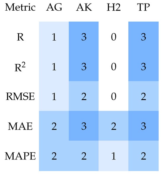
Figure 11. Heatmap of significant differences for FLAML vs. other frameworks. AG = AutoGluon; AK = AutoKeras; FL = FLAML; H2 = H2O; TP = TPOT.

Figure 12. Heatmap of significant differences for H2O vs. other frameworks. AG = AutoGluon; AK = AutoKeras; FL = FLAML; H2 = H2O; TP = TPOT.

Figure 13. Heatmap of significant differences for TPOT vs. other frameworks. AG = AutoGluon; AK = AutoKeras; FL = FLAML; H2 = H2O; TP = TPOT.

Across several datasets, AutoKeras consistently exhibited significant performance advantages relative to other frameworks, particularly AutoGluon. D4 and D10 exhibited the largest number of significant differences, encompassing nearly all framework combinations and metrics, suggesting that performance divergence was more pronounced in these datasets. D1, D3, and, in some cases, D5 and D6 (depending on the metric) showed few or no significant differences, suggesting more comparable performance between frameworks.

In summary, Dunn’s test confirms that the observed differences between frameworks are not random, with AutoKeras and AutoGluon being most frequently involved in significant differences across the analyzed datasets and metrics. Across virtually all datasets exhibiting statistical significance, three models (H2O, FLAML, and TPOT) consistently formed a homogeneous performance group. These models rarely demonstrated statistically significant differences among themselves, suggesting comparable optimization capabilities and robustness across diverse forecasting scenarios.

Although the AutoML frameworks achieved strong overall performance, some datasets exhibited lower predictive accuracy, particularly D2 and D6. These datasets contain heterogeneous laboratory procedures, limited sample sizes, and higher variability in both soil characteristics and stabilizer reactions, which likely increased experimental noise. Under such conditions, the models tended to overfit or produce unstable patterns, indicating that predictive performance is strongly dependent on data consistency and the representativeness of the experimental campaign.

3.3. Comparative Performance Indexes

To provide a unified measure of model performance across multiple regression metrics, we introduce a composite Performance Index (PI). PI serves as a comprehensive metric to evaluate the overall efficacy of predictive models by aggregating the performance indicators in Table 8. This composite balances correlation and error, yielding a single, interpretable score that indicates superior model performance, with higher values indicating better performance.

The PI is then calculated as the arithmetic mean of these normalized values:

$$\mathrm{PI}={\displaystyle \frac{w_1·R+w_2·R^2+w_3·\left(1-\frac{\mathrm{RMSE}}{{\mathrm{RMSE}}_{max}}\right)+w_4·\left(1-\frac{\mathrm{MAE}}{{\mathrm{MAE}}_{max}}\right)+w_5·\left(1-\frac{\mathrm{MAPE}/100}{{\mathrm{MAPE}}_{max}/100}\right)}{5}}$$

where $w_i$ is the weight associated with the performance measure, ${\mathrm{metric}}_{max}$ is the maximum observed value for that metric across all models on the dataset, representing the worst-case performance. To provide a holistic and unified measure of model performance across multiple regression metrics, the weights were set to 0.20, resulting in a simple arithmetic average for aggregation.

Table 11 summarizes the mean PI scores, along with their standard deviations, for five prominent AutoML frameworks across ten distinct datasets (D1 to D10). These scores are computed from multiple runs to account for variability in model training and optimization. The best results in each dataset comparison are highlighted in boldface. Moreover, Table 12 provides a summary listing, for each employed dataset, of the AutoML framework that achieved the highest averaged PI value.

Table 11. Average PI scores and standard deviations computed over 30 runs for each AutoML framework across all datasets. Boldface entries indicate the best results.

Dataset	AutoGluon	AutoKeras	FLAML	H2O	TPOT
D1	0.486 (±0.148)	0.498 (±0.136)	0.536 (±0.182)	0.581 (±0.121)	0.451 (±0.146)
D2	0.610 (±0.082)	0.706 (±0.072)	0.625 (±0.076)	0.578 (±0.184)	0.676 (±0.067)
D3	0.797 (±0.111)	0.787 (±0.156)	0.808 (±0.062)	0.829 (±0.064)	0.801 (±0.106)
D4	0.892 (±0.049)	0.413 (±0.197)	0.931 (±0.046)	0.944 (±0.028)	0.923 (±0.054)
D5	0.667 (±0.143)	0.748 (±0.134)	0.748 (±0.117)	0.685 (±0.151)	0.625 (±0.173)
D6	0.764 (±0.069)	0.676 (±0.150)	0.802 (±0.074)	0.800 (±0.076)	0.780 (±0.079)
D7	0.894 (±0.049)	0.831 (±0.079)	0.897 (±0.056)	0.847 (±0.208)	0.833 (±0.088)
D8	0.788 (±0.089)	0.792 (±0.112)	0.741 (±0.092)	0.687 (±0.243)	0.746 (±0.100)
D9	0.786 (±0.093)	0.778 (±0.082)	0.810 (±0.091)	0.716 (±0.199)	0.684 (±0.128)
D10	0.954 (±0.017)	0.927 (±0.022)	0.950 (±0.013)	0.850 (±0.223)	0.972 (±0.014)

Table 12. Summary of the top-performing AutoML frameworks per dataset and their averaged PI.

Dataset	Top-Performing Framework	PI (Average Value)
D1	H2O	0.581
D2	AutoKeras	0.706
D3	H2O	0.829
D4	H2O	0.944
D5	FLAML	0.748
D6	FLAML	0.802
D7	FLAML	0.897
D8	AutoKeras	0.792
D9	FLAML	0.810
D10	TPOT	0.972

An examination of the results presented in Table 11 and Table 12 shows clear patterns in the performance of the AutoML frameworks. Among the evaluated systems, FLAML achieved the highest average PI score, with a mean of 0.7848. The relatively small standard deviations, averaging around 0.0809, indicate stable behavior and efficient search procedures. FLAML presented superior performance, particularly on datasets with more samples, such as D5, D6, D7, and D9, suggesting that its strategy tends to extract better predictive performance from larger datasets. In contrast, AutoKeras showed greater performance fluctuations, with a lower mean PI of 0.7156 and a marked drop in D4 (0.413). This behavior may stem from its strong focus on neural architecture search, which might not adapt equally well to tabular data. AutoGluon, H2O, and TPOT achieved intermediate performance, with average PI scores of 0.7638, 0.7517, and 0.7491, respectively.

The statistical correlations identified between specific features and the UCS are underpinned by well-established physical and chemical mechanisms in soil mechanics, which lend credibility to the models’ predictions and enhance their practical utility. For instance, the high importance of stabilizer content (as cement, lime, and GGBS) is a direct reflection of the cementation process, in which hydration and pozzolanic reactions generate binding compounds such as calcium silicate hydrate (C-S-H) that form a rigid matrix between soil particles, thereby drastically improving shear strength. Similarly, the influence of curing time is physically justified, as it reflects the time-dependent progression of these chemical reactions, leading to a more mature, robust cemented structure.

The relevance of compaction parameters, such as Maximum Dry Density (MDD), is rooted in the principle of particle packing: a denser soil skeleton has fewer voids and closer grain contacts, providing a more effective framework for cementitious bonds to develop. Furthermore, the importance of clay content and plasticity index reflects the complex soil-binder interaction, in which clay minerals provide reactive surfaces for reactions but also demand higher water and stabilizer content, a nonlinear trade-off that the models appear to capture.

The prominence of calcium carbonate content (FCA) in the MICP-treated dataset (D9) is a quintessential example of a direct microstructural mechanism, where the precipitated calcite acts as the primary cementing agent, directly filling pores and bridging particles. Therefore, AutoML frameworks are not merely identifying abstract statistical patterns but are effectively learning the fundamental geotechnical principles that govern soil strength, moving predictions from a black-box correlation to a physically interpretable and practically valuable tool for engineering design.

3.4. Comparison with Previous Studies

When focusing only on datasets D1 to D6, the model proposed by Goliatt et al. [71] shows superior performance compared to the other approaches. In a separate comparison, when all datasets are considered, excluding Goliatt et al. [71], the AutoML frameworks generally achieve better predictive performance than the best models reported in the original reference studies, as shown in Table 13. In the latter table, we assigned binary scores to each AutoML framework based on whether it outperformed the reference model from the original study for each performance metric across the majority of the datasets. In particular, for each dataset and metric, we compared the framework’s mean value computed over our 30 independent runs to the best result reported in the corresponding reference. A score of “1” indicates that the framework’s average performance exceeded the reference in the majority of datasets for that metric. In contrast, “0” indicates it did not. Moreover, the row labeled “AutoML” corresponds to the sum of these binary scores obtained by all AutoML frameworks employed in this study (i.e., AutoGluon, AutoKeras, FLAML, H2O, and TPOT) for each metric. In contrast, the row labeled “Ref.” represents the number of datasets in which the reference studies reported the best results for each metric. Finally, the column labeled “Score” reports the total score across all metrics, thereby providing an overall measure of how frequently each framework outperformed the reference models.

Table 13. Binary performance comparison between AutoML frameworks and reference models. A score of 1 indicates that the framework outperformed the reference model for that metric on the majority of datasets, whereas 0 indicates it did not. The “Score” column denotes the total number of metrics for which each framework outperformed the reference models considered.

Model/Framework	R	R2	RMSE	MAE	MAPE	Score
AutoGluon	0	0	0	0	0	0
AutoKeras	0	1	0	1	1	3
FLAML	1	1	2	1	1	6
H2O	0	1	2	1	0	4
TPOT	1	0	1	1	0	3
AutoML	2	3	5	4	2	16
Ref.	3	3	4	3	2	15

The feature-importance analysis revealed that variables directly associated with soil composition and stabilizer dosage were consistently the most influential across the datasets. For lime- and cement-stabilized soils, stabilizer content, curing time, and Atterberg limits contributed most to model predictions. In geopolymer datasets, the alkali–binder ratio and molar concentration dominated the predictive structure. These trends are geotechnically consistent and indicate that the AutoML frameworks captured physically meaningful soil–stabilizer interactions.

3.5. Interpretation of the Findings

When evaluated together, the metrics provide a more comprehensive perspective on the framework’s performance. While R² and R capture the overall quality of fit, the absolute error metrics (RMSE and MAE) showed very similar values across datasets, suggesting robustness to outliers.

The relative error metric (MAPE) tended to produce inflated values when actual and predicted values were close to zero. This pattern was particularly evident in datasets D1, D2, D5, and D6, and was most pronounced in D10. In this context, dataset D4 yielded the most favorable MAPE across models, although AutoKeras again underperformed.

The frameworks generally achieved strong results for R², R, and MAPE. Furthermore, an inverse relationship was observed between R/R² and RMSE/MAE/MAPE, with higher R/R² values corresponding to lower RMSE/MAE/MAPE.

The findings indicate that, although the frameworks differ substantially in their ability to capture the linear relationship and the explained variance of the predictions, they perform comparably when evaluated using absolute and relative error metrics. The non-parametric statistical tests support this interpretation: the Kruskal–Wallis test detected significant differences only for R and R², and Dunn’s post hoc analysis revealed that these differences were primarily driven by the underperformance of AutoKeras relative to the other frameworks. In contrast, no statistically significant differences were observed in RMSE, MAE, or MAPE, indicating that AutoGluon, FLAML, H2O, and TPOT achieve comparable error magnitudes. This reinforces the notion that different AutoML approaches may converge to similar predictive errors, even when their capacity to explain data variability diverges substantially.

The strong results obtained by the model of Goliatt et al. [71] on datasets D1 to D6 highlight the substantial impact of careful model selection and systematic hyperparameter optimization on the predictive performance of UCS.

Based on the mean PI scores observations (Table 11), we recommend FLAML for applications requiring high overall performance and adaptability across varied datasets. For scenarios where computational resources are constrained or interpretability is prioritized, TPOT may serve as a viable alternative due to its balanced efficiency. H2O performs particularly well in complex datasets, such as D1, D3, D4 and D6, where PI scores exceed 0.94, suggesting effective handling of diverse data characteristics. Based on the runtime observations (Figure 8), AutoGluon is suitable for cases where a fast solution is required and the predictive performance for UCS is not the main priority. Future work could explore hybrid approaches that combine the strengths of these frameworks to further enhance the efficacy of AutoML.

3.6. Feature Importance Analysis

Figure 14, Figure 15, Figure 16, Figure 17 and Figure 18 show the averaged feature importance for datasets D1 through D10.

Figure 14. Averaged feature importance for datasets D1 and D2.

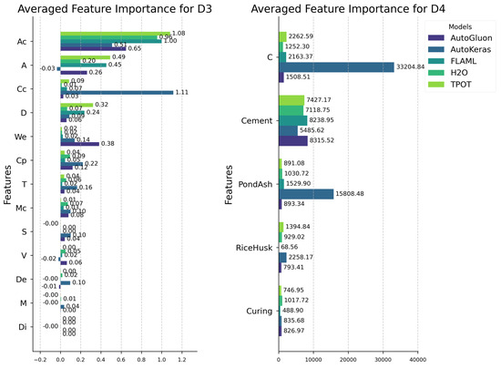
Figure 15. Averaged feature importance for datasets D3 and D4.

Figure 16. Averaged feature importance for datasets D5 and D6.

Figure 17. Averaged feature importance for datasets D7 and D8.

Figure 18. Averaged feature importance for datasets D9 and D10.

Features related to the number of stabilizers used in the samples occur more frequently in datasets D1, D2, D3, D4, D5, and D9, followed by features linked to soil moisture in datasets D6 and D7.

In dataset D1, the consistently high selection frequency of ‘Lime’ suggests that H2O’s performance might improve by refocusing the model on this feature. For dataset D2, TPOT consistently selected the feature ‘Cement’ at a high frequency. Likewise, in dataset D3, AutoKeras frequently selected the feature ‘Curing condition’. A similar pattern is observed with AutoKeras in dataset D4, where a high frequency of feature selection (‘Clay content’ and ‘Pondash content’) was accompanied by low performance compared to the other frameworks (Table 11).

An analysis of feature selection for dataset D5 (Figure 16) and the corresponding results (Table 11) indicate that feature selection alone does not account for the framework’s performance. Although AutoKeras and FLAML achieved comparable predictive accuracy, their selected feature sets differed substantially. This suggests that the model’s search space and optimization strategy also play a significant role in forecasting soil UCS.

In dataset D6, the frameworks with the highest PI values, FLAML and H2O, prioritized the feature ‘Optimum moisture content’ over ‘Maximum dry density’. This interpretation is reinforced by the fact that AutoKeras did not select the best moisture content and showed lower performance. In dataset D7, there is a clear relation between feature selection frequency and model performance. AutoGluon achieved the second-highest performance without selecting ‘Dry unit weight’ as often, whereas FLAML, which achieved the best PI, selected this feature more often.

In dataset D8, the low selection frequency of ‘Porosity’ seems to have penalized the results of H2O (where n in Figure 17 denotes ‘Porosity’, as reported in Section 2.1). In dataset D9, the limited selection of ‘Calcium carbonate content’ and ‘Median grain size’ appears to have influenced the observed variability in the H2O outcomes. In dataset D10, the consistently high selection frequency of ‘Cement proportion’ suggests that TPOT’s performance could improve by refocusing the modeling on this feature.

The differences observed in feature selection across models can be better understood by considering the geotechnical relationships among the soil parameters included in the datasets. Variables such as moisture content, dry density, porosity and plasticity are not independent descriptors of soil behavior. Soil moisture affects clayey soil conditions, pore water distribution and compaction results, which in turn influence soil dry density. As a result, soil moisture and density capture complementary aspects of the physical process, and both can serve as valid predictors of strength. This means that slight variations in the correlation structure of the dataset or slight differences in the optimization strategies of the frameworks may lead one model to select moisture content as the primary descriptor. In contrast, another may assign greater relevance to density or plasticity.

These relationships are particularly relevant given that geotechnical datasets often exhibit multicollinearity. Moisture-driven changes in soil structure alter density, stiffness and suction, creating groups of variables that convey similar physical information. This implies that different models may rely on different but equally meaningful representations of the exact mechanism. Nguyen et al. [119] highlight that high-dimensional material datasets frequently contain correlated or oversimplified variables, which encourages machine learning algorithms to identify alternative predictors that describe the same underlying material behavior. This observation is consistent with the role of moisture, density and related parameters in compacted soils, where several inputs express the effects of pore fluid distribution and particle rearrangement.

Differences in feature selection are also influenced by how each algorithm interprets nonlinearities and interactions among variables. Tree-based methods prioritize features that yield strong local partitions, making them sensitive to small changes in moisture or density that can significantly alter the decision boundaries. Linear and regularized models, on the other hand, tend to emphasize variables that maintain consistent global relationships with the target, which may favor density in some datasets and moisture in others. Oo et al. [120] show that feature-importance rankings can vary substantially across algorithms when correlated predictors are present, since each method captures distinct aspects of the latent structure revealed through interpretability tools such as SHAP. Their findings reinforce the expectation that model-dependent feature prioritization is expected in datasets with multiple variables describing interconnected physical phenomena.

For these reasons, the discrepancies documented in this study do not indicate instability or inconsistency in the predictive frameworks. Instead, they reflect the inherent multicollinearity in geotechnical materials and the different strategies that machine learning algorithms use to model nonlinear relationships. When multiple soil parameters encode different expressions of the exact physical mechanism, the models may select different predictors while still achieving comparable predictive performance. This behavior demonstrates that the frameworks are capturing the essential geotechnical processes governing the evolution of UCS, even when they prioritize different but physically related input variables.

3.7. Strengths and Limitations

The comparative analysis of AutoML frameworks highlighted distinct strengths and weaknesses. FLAML consistently ranked as the most reliable framework, delivering superior results across several datasets. This was most evident in metrics R, R², and RMSE, where the Kruskal–Wallis and Dunn’s tests confirmed its advantage over competitors.

FLAML reached competitive accuracy and produced consistent predictions in medium-sized datasets. In contrast, AutoKeras performed worse than the other frameworks, particularly on datasets with more variables. Both descriptive statistics and inferential tests supported this outcome: the Kruskal–Wallis test identified significant differences for R and R², and Dunn’s post hoc analysis linked these differences primarily to AutoKeras. Even so, AutoKeras occasionally achieved favorable MAPE results, suggesting some usefulness when relative rather than absolute error is the primary focus.

AutoGluon achieved stable results across most datasets, particularly when the target variable showed high variability. H2O also performed well in R and R², but its higher MAPE values in some datasets indicate limitations in contexts where percentage-based error is a key concern. TPOT’s genetic programming strategy produced pipelines with robust predictive performance, reflected in its overall high aggregated Performance Index (PI) scores, particularly for dataset D10 (0.972).

Although AutoGluon and AutoKeras quickly reach a solution, there is no option to improve predictive performance for UCS by extending the execution time. TPOT, in contrast, can produce reliable, consistent results for UCS prediction, but it requires a long execution time to converge.

Furthermore, AutoML frameworks exhibit inherent limitations in their sensitivity to data quality [121,122]. Indeed, the latter tools are highly dependent on clean, well-structured input data, as they typically employ automated preprocessing that may not adequately handle domain-specific data anomalies or complex feature interactions unique to geotechnical applications. While the frameworks leveraged in the present study employed basic preprocessing routines, specialized domain knowledge remains essential for ensuring appropriate feature engineering and handling of geotechnical measurement artifacts, as is incidentally the case in other domains as well [70].

In addition to data sensitivity, AutoML frameworks can be computationally intensive, particularly when exploring complex model spaces or with large datasets [123,124]. The resource requirements vary significantly across frameworks, with TPOT and AutoKeras generally requiring more computational resources than the lighter FLAML approach. The latter considerations highlight that AutoML should be viewed as a complementary tool rather than a complete replacement for expert-driven modeling, specifically in scenarios with limited computational resources or complex domain-specific data challenges [124].

The results indicate that although AutoML frameworks vary in their capacity to capture variance and linear relationships, their predictive errors converge when evaluated with RMSE, MAE, and MAPE. This suggests that, in practice, the choice of framework may be guided more by the characteristics of the dataset and the prediction goals rather than by absolute error values. Despite the discussed constraints, the frameworks analyzed in the present work can support decision-making by providing automated UCS predictions. They reduce both the time required for model training and for prediction, while lowering the entry barrier for researchers with a limited ML background.

4. Concluding Remarks

This study investigated the application of AutoML frameworks to predict the unconfined compressive strength (UCS) of stabilized soils using datasets collected worldwide. The analysis evaluated the predictive performance of five state-of-the-art AutoML frameworks across various soil types, stabilizers, and experimental conditions, including traditional stabilizers such as cement and lime, as well as alternative materials such as rice husk ash, geopolymer binders, and biochemically treated soils. The datasets compiled from multiple countries enabled a comprehensive assessment of the model’s generalizability and robustness.

Despite promising results from AutoML frameworks for UCS prediction, their use is most suitable for research contexts that do not demand the highest levels of accuracy and performance. Superior results can be achieved through the careful selection, customization, and hyperparameter tuning of ML models, as evidenced by the work of Goliatt et al. [71]. However, AutoML frameworks effectively fulfill their intended purpose of automatically training and predicting UCS through ML models, reducing the barrier to entry for researchers with limited technical expertise in this domain [109]. They provide a systematic and reproducible approach to handling heterogeneous datasets, minimizing manual intervention in feature engineering, model selection, and hyperparameter optimization.

The findings have several important implications for predicting UCS in geotechnical engineering. First, AutoML enables rapid, automated development of predictive models, significantly reducing reliance on time-consuming and resource-intensive laboratory experiments. Second, by applying these frameworks to datasets from multiple regions, the study demonstrates that AutoML can generate consistent and generalizable insights into soil–stabilizer interactions, supporting more informed design and decision-making in soil stabilization projects. Third, the comparative analysis of multiple AutoML frameworks provides practical guidance for selecting suitable tools for future UCS prediction tasks, highlighting their relative strengths and limitations.

A comparative evaluation revealed that all frameworks delivered reasonable predictive accuracy; however, notable differences were observed depending on the dataset characteristics and experimental conditions. FLAML achieved the highest average composite Performance Index (PI) score (0.7848) across the datasets and performed competitively on medium-sized datasets. TPOT stood out for consistently achieving robust performance across diverse datasets, demonstrating particular strength in handling complex interactions between soil and stabilizers, and performing best on correlation-based metrics in statistical comparisons. AutoGluon and H2O also achieved high predictive performance for larger datasets with nonlinear relationships. In contrast, AutoKeras exhibited lower accuracy, particularly on higher-dimensional datasets, a finding reinforced by statistical tests that highlighted its comparative underperformance.

We provide targeted recommendations based on the observed trade-offs between accuracy and computational efficiency. When computational speed and efficiency are paramount, FLAML is the superior choice, as it is ideally suited for rapid prototyping and preliminary studies, delivering strong results on medium-sized datasets in a minimal time. For practitioners who prioritize a straightforward, robust, and easily deployable solution without deep ML expertise, AutoGluon offers a robust “out of the box” experience, often achieving top-tier performance through its sophisticated ensemble methods.

While H2O provides a reliable enterprise-grade option and AutoKeras caters to specific neural network-focused applications, TPOT and FLAML emerge as the most versatile and practical frameworks for the diverse datasets typical of geotechnical engineering. Ultimately, when computational speed is prioritized, AutoGluon is the optimal choice, delivering competitive predictive performance on larger datasets with nonlinear relationships through its sophisticated ensemble methods. This practical guidance empowers geotechnical professionals to effectively leverage AutoML, thus accelerating data-driven decision-making in soil stabilization projects. Nevertheless, practitioners must be aware of AutoML’s related limitations, including sensitivity to data quality, substantial computational requirements for comprehensive searches, and potential oversimplification of domain-specific data relationships that may benefit from expert feature engineering.

Future research should move beyond internal cross-validation and explicitly evaluate the cross-dataset transferability of AutoML models for UCS prediction. However, in the present study, the analysis is intentionally restricted to within-dataset modeling, so that each experimental dataset defines a local prediction task and no single global AutoML model is calibrated on the merged data. Transfer learning strategies [125,126] represent a promising direction because they allow a model trained on a large or heterogeneous source dataset to be efficiently fine-tuned for new experimental conditions or geographical regions. This is particularly relevant considering the diversity of soils, stabilizers, and locations represented in the datasets used in this study (D1 to D10). Future investigations may also benefit from expanding the size and variability of available datasets and from incorporating additional physical descriptors, including curing-related parameters that influence strength development. Additional studies could evaluate a broader set of AutoML frameworks, as suggested by [100], and examine whether extended training times lead to improvements in predictive performance, allowing more robust comparisons with the findings reported by Goliatt et al. [71]. Together, these research directions contribute to a deeper understanding of the generalization capacity of AutoML approaches and support their application across a wider range of geotechnical contexts.

This study demonstrates that AutoML frameworks can effectively automate UCS prediction while offering accessibility and reproducibility for researchers. Although not a replacement for carefully tailored ML approaches in high-accuracy contexts, they represent a valuable tool for accelerating research and supporting data-driven design of soil stabilization.

References

- Sheshde, E.A.; Cheshomi, A. New method for estimating unconfined compressive strength (UCS) using small rock samples. J. Pet. Sci. Eng. 2015, 133, 367–375. [Google Scholar] [CrossRef]
- Kormu, S.; Sorsa, A.; Amena, S. Correlation of unconfined compressive strength (UCS) with compaction characteristics of soils in Burayu Town. Adv. Mater. Sci. Eng. 2022, 2022, 1548272. [Google Scholar] [CrossRef]
- Tran, V.Q.; Nguyen, L.Q. Using machine learning technique for designing reinforced lightweight soil. J. Intell. Fuzzy Syst. 2022, 43, 1633–1650. [Google Scholar] [CrossRef]
- Consoli, N.C.; Leon, H.B.; da Silva Carretta, M.; Daronco, J.V.L.; Lourenço, D.E. The effects of curing time and temperature on stiffness, strength and durability of sand-environment friendly binder blends. Soils Found. 2019, 59, 1428–1439. [Google Scholar] [CrossRef]
- Zhang, Y.; Jiang, S.; Quan, D.; Fang, K.; Wang, B.; Ma, Z. Properties of Sustainable Earth Construction Materials: A State-of-the-Art Review. Sustainability 2024, 16, 670. [Google Scholar] [CrossRef]
- Eyo, E.; Abbey, S. Machine learning regression and classification algorithms utilised for strength prediction of OPC/by-product materials improved soils. Constr. Build. Mater. 2021, 284, 122817. [Google Scholar] [CrossRef]
- Behak, L. Soil Stabilization with Rice Husk Ash. In Rice; Amanullah, K., Fahad, S., Eds.; IntechOpen: Rijeka, Croatia, 2017; Chapter 3. [Google Scholar] [CrossRef]
- Soleimani, S.; Rajaei, S.; Jiao, P.; Sabz, A.; Soheilinia, S. New prediction models for unconfined compressive strength of geopolymer stabilized soil using multi-gen genetic programming. Measurement 2018, 113, 99–107. [Google Scholar] [CrossRef]
- Gajurel, A.; Mukherjee, P.S.; Chittoori, B. Estimating Optimal Additive Content for Soil Stabilization Using Machine Learning Methods. In Proceedings of the 8th International Conference on Case Histories in Geotechnical Engineering: Geotechnical Materials, Modeling, and Testing, Geo-Congress 2019, Philadelphia, PA, USA, 24–27 March 2019; pp. 662–672. [Google Scholar] [CrossRef]
- Saad, A.H.; Nahazanan, H.; Yusuf, B.; Toha, S.F.; Alnuaim, A.; El-Mouchi, A.; Elseknidy, M.; Mohammed, A.A. A Systematic Review of Machine Learning Techniques and Applications in Soil Improvement Using Green Materials. Sustainability 2023, 15, 9738. [Google Scholar] [CrossRef]
- Khatti, J.; Grover, K.S. A Scientometrics Review of Soil Properties Prediction Using Soft Computing Approaches. Arch. Comput. Methods Eng. 2023, 31, 1519–1553. [Google Scholar] [CrossRef]
- Zhang, G.; Chen, C.; Sun, J.; Li, K.; Xiao, F.; Wang, Y.; Chen, M.; Huang, J.; Wang, X. Mixture optimisation for cement-soil mixtures with embedded GFRP tendons. J. Mater. Res. Technol. 2022, 18, 611–628. [Google Scholar] [CrossRef]
- Mohanty, S.; Roy, N.; Singh, S.P.; Sihag, P. Estimating the strength of stabilized dispersive soil with cement clinker and fly ash. Geotech. Geol. Eng. 2019, 37, 2915–2926. [Google Scholar] [CrossRef]
- Zhang, G.; Ding, Z.; Wang, Y.; Fu, G.; Wang, Y.; Xie, C.; Zhang, Y.; Zhao, X.; Lu, X.; Wang, X. Performance prediction of cement stabilized soil incorporating solid waste and propylene fiber. Materials 2022, 15, 4250. [Google Scholar] [CrossRef] [PubMed]
- Chen, H.; Zhang, L. A machine learning-based method for predicting end-bearing capacity of rock-socketed shafts. Rock Mech. Rock Eng. 2022, 55, 1743–1757. [Google Scholar] [CrossRef]
- Kayadelen, C.; Altay, G.; Önal, Y. Numerical simulation and novel methodology on resilient modulus for traffic loading on road embankment. Int. J. Pavement Eng. 2021, 23, 3212–3221. [Google Scholar] [CrossRef]
- Ly, H.B.; Phaim, B.T. Soil unconfined compressive strength prediction using random forest (RF) machine learning model. Open Constr. Build. Technol. J. 2020, 14, 278–285. [Google Scholar] [CrossRef]
- Van Giap, L.; Pham, T.A.; Vu, H.L. Application of random forest model to determine unconfined compressive strength of the soil-cement mixture. In Proceedings of the CIGOS 2021, Ha Long, Vietnam, 28–29 October 2021. [Google Scholar] [CrossRef]
- Suman, S.; Mahamaya, M.; Das, S.K. Prediction of maximum dry density and unconfined compressive strength of cement stabilised soil using artificial intelligence techniques. Int. J. Geosynth. Ground Eng. 2016, 2, 11. [Google Scholar] [CrossRef]
- Tinoco, J.; Alberto, A.; Oliveira, P.J.V.; Lemos, L.; Correia, A.G. Data-driven approach to predict unconfined compressive strength of laboratory soil stabilized with cementitious binders. In Proceedings of the 17th European Conference on Soil Mechanics and Geotechnical Engineering, ECSMGE 2019, Reykjavik, Iceland, 1–6 September 2019. [Google Scholar]
- Tinoco, J.; Alberto, A.; da Venda, P.; Gomes Correia, A.; Lemos, L. A novel approach based on soft computing techniques for unconfined compressive strength prediction of soil cement mixtures. Neural Comput. Appl. 2020, 32, 8985–8991. [Google Scholar] [CrossRef]
- Jalal, F.E.; Xu, Y.; Iqbal, M.; Javed, M.F.; Jamhiri, B. Predictive modeling of swell strength of expansive soils using artificial intelligence approaches: ANN, ANFIS and GEP. J. Environ. Manag. 2021, 289, 112420. [Google Scholar] [CrossRef]
- Pham, V.N.; Oh, E.; Ong, D.E. Effects of binder types and other significant variables on the unconfined compressive strength of chemical-stabilized clayey soil using gene-expression programming. Neural Comput. Appl. 2022, 34, 9103–9121. [Google Scholar] [CrossRef]
- Tran, V.Q. Selection of single machine learning model for designing compressive strength of stabilized soil containing lime, cement and bitumen. J. Intell. Fuzzy Syst. 2023, 45, 239–256. [Google Scholar] [CrossRef]
- Guo, P.; Meng, W.; Xu, M.; Li, V.C.; Bao, Y. Predicting mechanical properties of high-performance fiber-reinforced cementitious composites by integrating micromechanics and machine learning. Materials 2021, 14, 3143. [Google Scholar] [CrossRef] [PubMed]
- Tao, H.; Habib, M.; Aljarah, I.; Faris, H.; Afan, H.A.; Yaseen, Z.M. An intelligent evolutionary extreme gradient boosting algorithm development for modeling scour depths under submerged weir. Inform. Sci. 2021, 570, 172–184. [Google Scholar] [CrossRef]
- Ding, X.; Amiri, M.; Hasanipanah, M. Enhancing shear strength predictions of rocks using a hierarchical ensemble model. Sci. Rep. 2024, 14, 20268. [Google Scholar] [CrossRef] [PubMed]
- Malik, A.; Saggi, M.K.; Rehman, S.; Sajjad, H.; Inyurt, S.; Bhatia, A.S.; Farooque, A.A.; Oudah, A.Y.; Yaseen, Z.M. Deep learning versus gradient boosting machine for pan evaporation prediction. Eng. Appl. Comput. Fluid Mech. 2022, 16, 570–587. [Google Scholar] [CrossRef]
- Faridmehr, I.; Shariq, M.; Plevris, V.; Aalimahmoody, N. Novel hybrid informational model for predicting the creep and shrinkage deflection of reinforced concrete beams containing GGBFS. Neural Comput. Appl. 2022, 34, 13107–13123. [Google Scholar] [CrossRef]
- Tao, H.; Awadh, S.M.; Salih, S.Q.; Shafik, S.S.; Yaseen, Z.M. Integration of extreme gradient boosting feature selection approach with machine learning models: Application of weather relative humidity prediction. Neural Comput. Appl. 2022, 34, 515–533. [Google Scholar] [CrossRef]
- Ghanizadeh, A.R.; Heidarabadizadeh, N.; Bayat, M.; Khalifeh, V. Modeling of unconfined compressive strength and Young’s modulus of lime and cement stabilized clayey subgrade soil using evolutionary polynomial regression (EPR). Int. J. Min. Geo-Eng. 2022, 56, 257–269. [Google Scholar]
- Tran, V.Q. Hybrid gradient boosting with meta-heuristic algorithms prediction of unconfined compressive strength of stabilized soil based on initial soil properties, mix design and effective compaction. J. Clean. Prod. 2022, 355, 131683. [Google Scholar] [CrossRef]
- Dehghanbanadaki, A. Intelligent modelling and design of soft soil improved with floating column-like elements as a road subgrade. Transp. Geotech. 2021, 26, 100428. [Google Scholar] [CrossRef]
- Wang, J.; Xing, Y.; Cheng, L.; Qin, F.; Ma, T. The prediction of mechanical properties of cement soil based on PSO-SVM. In Proceedings of the 2010 International Conference on Computational Intelligence and Software Engineering, CiSE 2010, Wuhan, China, 10–12 December 2010. [Google Scholar]
- Shamshirband, S.; Tavakkoli, A.; Roy, C.B.; Motamedi, S.; Song, K.I.; Hashim, R.; Islam, S.M. Hybrid intelligent model for approximating unconfined compressive strength of cement-based bricks with odd-valued array of peat content (0–29%). Powder Technol. 2015, 284, 560–570. [Google Scholar] [CrossRef]
- Zhang, G.; Chen, C.; Li, K.; Xiao, F.; Sun, J.; Wang, Y.; Wang, X. Multi-objective optimisation design for GFRP tendon reinforced cemented soil. Constr. Build. Mater. 2022, 320, 126297. [Google Scholar] [CrossRef]
- He, P.; Di, H.; He, C.; Zhang, X.; Liu, C.; Zhou, S. Spatio-temporal graph convolutional networks with multi-source fusion for predicting excavation deformation. Adv. Eng. Inform. 2025, 68, 103722. [Google Scholar] [CrossRef]
- He, P.; Guo, H.; Di, H.; Guan, Z. Application of soil parameter back analysis method based on MLAPSO in staged excavation deformation prediction. Expert Syst. Appl. 2025, 259, 129244. [Google Scholar] [CrossRef]
- Le, H.A.; Nguyen, T.A.; Nguyen, D.D.; Prakash, I. Prediction of soil unconfined compressive strength using artificial neural network model. Vietnam J. Earth Sci. 2020, 42, 255–264. [Google Scholar] [CrossRef]
- Ngo, A.Q.; Nguyen, L.Q.; Tran, V.Q. Developing interpretable machine learning Shapley additive explanations model for unconfined compressive strength of cohesive soils stabilized with geopolymer. PLoS ONE 2023, 18, e0286950. [Google Scholar] [CrossRef]
- Das, S.K.; Samui, P.; Sabat, A.K. Application of artificial intelligence to maximum dry density and unconfined compressive strength of cement stabilized soil. Geotech. Geol. Eng. 2011, 29, 329–342. [Google Scholar] [CrossRef]
- Güllü, H.; Fedakar, H.İ. On the prediction of unconfined compressive strength of silty soil stabilized with bottom ash, jute and steel fibers via artificial intelligence. Geomech. Eng. 2017, 12, 441–464. [Google Scholar] [CrossRef]
- Tinoco, J.; Correia, A.A.S.; da Venda, P. Soil–cement mixtures reinforced with fibers: A data-driven approach for mechanical properties prediction. Appl. Sci. 2021, 11, 8099. [Google Scholar] [CrossRef]
- Tiwari, N.; Satyam, N. Coupling effect of pond ash and polypropylene fiber on strength and durability of expansive soil subgrades: An integrated experimental and machine learning approach. J. Rock Mech. Geotech. Eng. 2021, 13, 1101–1112. [Google Scholar] [CrossRef]
- Yao, H.; Xu, Z.; Hou, Y.; Dong, Q.; Liu, P.; Ye, Z.; Pei, X.; Oeser, M.; Wang, L.; Wang, D. Advanced industrial informatics towards smart, safe and sustainable roads: A state of the art. J. Traffic Transp. Eng. (Engl. Ed.) 2023, 10, 143–158. [Google Scholar] [CrossRef]
- Ouf, M.S. Towards sustainability: Artificial intelligent based approach for soil stabilization using various pozzolans. WIT Trans. Ecol. Environ. 2012, 162, 253–262. [Google Scholar]
- Oda, K. Method for objectively determining design strength with artificial neural network. In Proceedings of the 16th Asian Regional Conference on Soil Mechanics and Geotechnical Engineering, ARC 2019, Taipei, Taiwan, 14–18 October 2019. [Google Scholar]
- Onyelowe, K.C.; Iqbal, M.; Jalal, F.E.; Onyia, M.E.; Onuoha, I.C. Application of 3-algorithm ANN programming to predict the strength performance of hydrated-lime activated rice husk ash treated soil. Multiscale Multidiscip. Model. Exp. Des. 2021, 4, 259–274. [Google Scholar] [CrossRef]
- Yang, X.; Guan, J.; Ding, L.; You, Z.; Lee, V.C.; Hasan, M.R.M.; Cheng, X. Research and applications of artificial neural network in pavement engineering: A state-of-the-art review. J. Traffic Transp. Eng. (Engl. Ed.) 2021, 8, 1000–1021. [Google Scholar] [CrossRef]
- Hoang, H.G.; Nguyen, T.A. An artificial intelligence approach to predict the resilient modulus of subgrade pavement or unbound material. In Proceedings of the CIGOS 2021, Ha Long, Vietnam, 28–29 October 2021. [Google Scholar] [CrossRef]
- Sezer, A.; Sezer, G.İ.; Mardani-Aghabaglou, A.; Altun, S. Prediction of mechanical and penetrability properties of cement-stabilized clay exposed to sulfate attack by use of soft computing methods. Neural Comput. Appl. 2020, 32, 16707–16722. [Google Scholar] [CrossRef]
- MolaAbasi, H.; Shooshpasha, I. Prediction of zeolite-cement-sand unconfined compressive strength using polynomial neural network. Eur. Phys. J. Plus 2016, 131, 108. [Google Scholar] [CrossRef]
- Rezazadeh Eidgahee, D.; Rafiean, A.H.; Haddad, A. A novel formulation for the compressive strength of IBP-based geopolymer stabilized clayey soils using ANN and GMDH-NN approaches. Iran J. Sci. Technol.-Trans. Civ. Eng. 2020, 44, 219–229. [Google Scholar]
- Sihag, P.; Suthar, M.; Mohanty, S. Estimation of UCS-FT of dispersive soil stabilized with fly ash, cement clinker and GGBS by artificial intelligence. Iran J. Sci. Technol.-Trans. Civ. Eng. 2021, 45, 901–912. [Google Scholar] [CrossRef]
- Dehghanbanadaki, A.; Sotoudeh, M.A.; Golpazir, I.; Keshtkarbanaeemoghadam, A.; Ilbeigi, M. Prediction of geotechnical properties of treated fibrous peat by artificial neural networks. Bull. Eng. Geol. Environ. 2019, 78, 1345–1358. [Google Scholar] [CrossRef]
- Javdanian, H.; Lee, S. Evaluating unconfined compressive strength of cohesive soils stabilized with geopolymer: A computational intelligence approach. Eng. Comput. 2019, 35, 191–199. [Google Scholar] [CrossRef]
- Kardani, N.; Zhou, A.; Shen, S.L.; Nazem, M. Estimating unconfined compressive strength of unsaturated cemented soils using alternative evolutionary approaches. Transp. Geotech. 2021, 29, 100591. [Google Scholar] [CrossRef]
- Gajurel, A.; Chittoori, B.; Mukherjee, P.S.; Sadegh, M. Machine learning methods to map stabilizer effectiveness based on common soil properties. Transp. Geotech. 2021, 27, 100506. [Google Scholar] [CrossRef]
- Iravanian, A.; Kassem, Y.; Gökçekuş, H. Stress–strain behavior of modified expansive clay soil: Experimental measurements and prediction models. Environ. Earth Sci. 2022, 81, 107. [Google Scholar] [CrossRef]
- Taffese, W.Z.; Abegaz, K.A. Prediction of compaction and strength properties of amended soil using machine learning. Buildings 2022, 12, 613. [Google Scholar] [CrossRef]
- Mojtahedi, S.F.F.; Ahmadihosseini, A.; Sadeghi, H. An artificial intelligence based data-driven method for forecasting unconfined compressive strength of cement stabilized soil by deep mixing technique. Geotech. Geol. Eng. 2023, 41, 491–514. [Google Scholar]
- Zhang, C.; Zhu, Z.; Liu, F.; Yang, Y.; Wan, Y.; Huo, W.; Yang, L. Efficient machine learning method for evaluating compressive strength of cement stabilized soft soil. Constr. Build. Mater. 2023, 392, 131887. [Google Scholar] [CrossRef]
- Choobbasti, A.J.; Kutanaei, S.S. Microstructure characteristics of cement-stabilized sandy soil using nanosilica. J. Rock Mech. Geotech. Eng. 2017, 9, 981–988. [Google Scholar] [CrossRef]
- Kang, X.; Ge, L.; Kang, G.C.; Mathews, C. Laboratory investigation of the strength, stiffness, and thermal conductivity of fly ash and lime kiln dust stabilised clay subgrade materials. Road Mater. Pavement Des. 2015, 16, 928–945. [Google Scholar] [CrossRef]
- Association, N.L. Technical Brief: Mixture Design and Testing Procedures for Lime Stabilized Soil; Technical Report; National Lime Association: Arlington, VA, USA, 2006. [Google Scholar]
- Association, P.C. Soil Cement Laboratory Handbook; Technical Report; Portland Cement Association: Washington, DC, USA, 1992. [Google Scholar]
- U.S. Army. Soil Stabilization for Pavements; Technical Report TM 5-882-14/AFM 32-1019; U.S. Army: Arlington, VA, USA, 1994. [Google Scholar]
- Sahin, E.K.; Demir, S. Greedy-AutoML: A novel greedy-based stacking ensemble learning framework for assessing soil liquefaction potential. Eng. Appl. Artif. Intell. 2023, 119, 105732. [Google Scholar] [CrossRef]
- Hutter, F.; Kotthoff, L.; Vanschoren, J. Automated Machine Learning: Methods, Systems, Challenges; Springer: Cham, Switzerland, 2019. [Google Scholar] [CrossRef]
- Al Alamin, M.A.; Uddin, G. How far are we with automated machine learning? characterization and challenges of AutoML toolkits. Empir. Softw. Eng. 2024, 29, 91. [Google Scholar] [CrossRef]
- Goliatt, L.; Marhoon, H.A.; Yaseen, Z.M.; Heddam, S.; Zand, A.W.A.; Halder, B.; Tan, M.L.; Sa’adi, Z.; Ahmadianfar, I.; Elsayed, S. An evolutionary optimized automated machine learning approach to soil unconfined compressive strength prediction for sustainable transportation infrastructure. Transp. Geotech. 2025, 52, 101550. [Google Scholar] [CrossRef]
- Wang, L. Automated machine learning techniques for estimating the unconfined compressive strength of soil stabilization. Int. J. Interact. Des. Manuf. (IJIDeM) 2025, 19, 6347–6359. [Google Scholar] [CrossRef]
- Ngo, T.Q.; Nguyen, L.Q.; Tran, V.Q. Novel hybrid machine learning models including support vector machine with meta-heuristic algorithms in predicting unconfined compressive strength of organic soils stabilised with cement and lime. Int. J. Pavement Eng. 2023, 24, 3191–3205. [Google Scholar] [CrossRef]
- Onyelowe, K.C.; Moghal, A.A.B.; Ebid, A.; Rehman, A.U.; Hanandeh, S.; Priyan, V. Estimating the strength of soil stabilized with cement and lime at optimal compaction using ensemble-based multiple machine learning. Sci. Rep. 2024, 14, 17400. [Google Scholar] [CrossRef]
- Teodoru, I.B.; Voinea, M.M.; Ene, A.D.; Mihai, G.O.; Dumitrescu, A.M.; Radu, D.G.; Chivu, A.P.; Radulescu, I.M. Prediction of Unconfined Compressive Strength in Cement-Treated Soils: A Machine Learning Approach. Appl. Sci. 2025, 15, 7022. [Google Scholar] [CrossRef]
- Yao, Q.; Lu, Y.; Yang, J.; Zhao, M. Hybrid XGB model for predicting unconfined compressive strength of solid waste-cement-stabilized cohesive soil. Constr. Build. Mater. 2024, 449, 138242. [Google Scholar] [CrossRef]
- ASTM D2487-06; Standard Practice for Classification of Soils for Engineering Purposes (Unified Soil Classification System). ASTM International: West Conshohocken, PA, USA, 2006. [CrossRef]
- Ngo, H.T.T.; Pham, T.A.; Vu, H.L.T.; Giap, L.V. Application of Artificial Intelligence to Determined Unconfined Compressive Strength of Cement-Stabilized Soil in Vietnam. Appl. Sci. 2021, 11, 1949. [Google Scholar] [CrossRef]
- Priyadarshee, A.; Chandra, S.; Gupta, D.; Kumar, V. Neural Models for Unconfined Compressive Strength of Kaolin clay mixed with pond ash, rice husk ash and cement. J. Soft Comput. Civ. Eng. 2020, 4, 85–102. [Google Scholar]
- Mozumder, R.A.; Laskar, A.I. Prediction of unconfined compressive strength of geopolymer stabilized clayey soil using Artificial Neural Network. Comput. Geotech. 2015, 69, 291–300. [Google Scholar] [CrossRef]
- Taffese, W.Z.; Abegaz, K.A. Artificial Intelligence for Prediction of Physical and Mechanical Properties of Stabilized Soil for Affordable Housing. Appl. Sci. 2021, 11, 7503. [Google Scholar] [CrossRef]
- Tabarsa, A.; Latifi, N.; Osouli, A.; Bagheri, Y. Unconfined compressive strength prediction of soils stabilized using artificial neural networks and support vector machines. Front. Struct. Civ. Eng. 2021, 15, 520–536. [Google Scholar] [CrossRef]
- Mahmoodzadeh, A.; Mohammadi, M.; Hashim Ibrahim, H.; Nariman Abdulhamid, S.; Ghafoor Salim, S.; Farid Hama Ali, H.; Kamal Majeed, M. Artificial intelligence forecasting models of uniaxial compressive strength. Transp. Geotech. 2021, 27, 100499. [Google Scholar] [CrossRef]
- Wang, H.L.; Yin, Z.Y. Unconfined compressive strength of bio-cemented sand: State-of-the-art review and MEP-MC-based model development. J. Clean. Prod. 2021, 315, 128205. [Google Scholar] [CrossRef]
- van Paassen, L.A.; Ghose, R.; van der Linden, T.J.M.; van der Star, W.R.L.; van Loosdrecht, M.C.M. Quantifying Biomediated Ground Improvement by Ureolysis: Large-Scale Biogrout Experiment. J. Geotech. Geoenviron. Eng. 2010, 136, 1721–1728. [Google Scholar] [CrossRef]
- Cheng, L.; Cord-Ruwisch, R.; Shahin, M.A. Cementation of sand soil by microbially induced calcite precipitation at various degrees of saturation. Can. Geotech. J. 2013, 50, 81–90. [Google Scholar] [CrossRef]
- Cheng, L.; Shahin, M.; Cord-Ruwisch, R. Bio-cementation of sandy soil using microbially induced carbonate precipitation for marine environments. Géotechnique 2014, 64, 1010–1013. [Google Scholar] [CrossRef]
- Cheng, L.; Shahin, M.A.; Mujah, D. Influence of Key Environmental Conditions on Microbially Induced Cementation for Soil Stabilization. J. Geotech. Geoenviron. Eng. 2017, 143, 04016083. [Google Scholar] [CrossRef]
- Zhao, Q.; Li, L.; Li, C.; Li, M.; Amini, F.; Zhang, H. Factors Affecting Improvement of Engineering Properties of MICP-Treated Soil Catalyzed by Bacteria and Urease. J. Mater. Civ. Eng. 2014, 26, 04014094. [Google Scholar] [CrossRef]
- Mahawish, A.; Bouazza, A.; Gates, W.P. Effect of particle size distribution on the bio-cementation of coarse aggregates. Acta Geotech. 2018, 13, 1019–1025. [Google Scholar] [CrossRef]
- Mahawish, A.; Bouazza, A.; Gates, W.P. Unconfined Compressive Strength and Visualization of the Microstructure of Coarse Sand Subjected to Different Biocementation Levels. J. Geotech. Geoenviron. Eng. 2019, 145, 04019033. [Google Scholar] [CrossRef]
- Mujah, D.; Cheng, L.; Shahin, M.A. Microstructural and Geomechanical Study on Biocemented Sand for Optimization of MICP Process. J. Mater. Civ. Eng. 2019, 31, 04019025. [Google Scholar] [CrossRef]
- Wen, K.; Li, Y.; Liu, S.; Bu, C.; Li, L. Development of an Improved Immersing Method to Enhance Microbial Induced Calcite Precipitation Treated Sandy Soil through Multiple Treatments in Low Cementation Media Concentration. Geotech. Geol. Eng. 2019, 37, 1015–1027. [Google Scholar] [CrossRef]
- Xiao, Y.; He, X.; Evans, T.M.; Stuedlein, A.W.; Liu, H. Unconfined Compressive and Splitting Tensile Strength of Basalt Fiber–Reinforced Biocemented Sand. J. Geotech. Geoenviron. Eng. 2019, 145, 04019048. [Google Scholar] [CrossRef]
- Nafisi, A.; Mocelin, D.; Montoya, B.M.; Underwood, S. Tensile strength of sands treated with microbially induced carbonate precipitation. Can. Geotech. J. 2020, 57, 1611–1616. [Google Scholar] [CrossRef]
- Wang, Y.; Soga, K.; Dejong, J.T.; Kabla, A.J. A microfluidic chip and its use in characterising the particle-scale behaviour of microbial-induced calcium carbonate precipitation (MICP). Géotechnique 2019, 69, 1086–1094. [Google Scholar] [CrossRef]
- James, G.; Witten, D.; Hastie, T.; Tibshirani, R. An Introduction to Statistical Learning: With Applications in R, 2nd ed.; Springer: New York, NY, USA, 2021; p. 607. [Google Scholar] [CrossRef]
- Eldeeb, H.; Maher, M.; Elshawi, R.; Sakr, S. AutoMLBench: A comprehensive experimental evaluation of automated machine learning frameworks. Expert Syst. Appl. 2024, 243, 122877. [Google Scholar] [CrossRef]
- He, X.; Zhao, K.; Chu, X. AutoML: A survey of the state-of-the-art. Knowl.-Based Syst. 2021, 212, 106622. [Google Scholar] [CrossRef]
- Baratchi, M.; Wang, C.; Limmer, S.; van Rijn, J.N.; Hoos, H.H.; Bäck, T.; Olhofer, M. Automated machine learning: Past, present and future. Artif. Intell. Rev. 2024, 57, 122. [Google Scholar] [CrossRef]
- Vakhrushev, A.; Ryzhkov, A.; Savchenko, M.; Simakov, D.; Damdinov, R.; Tuzhilin, A. LightAutoML: AutoML solution for a large financial services ecosystem. arXiv 2021, arXiv:2109.01528. [Google Scholar]
- Zhang, H.; Ji, J.; Liu, Z.; Lu, H.; Qian, C.; Wei, C.; Chen, S.; Lu, W.; Wang, C.; Xu, H.; et al. Artificial intelligence for the diagnosis of clinically significant prostate cancer based on multimodal data: A multicenter study. BMC Med. 2023, 21, 270. [Google Scholar] [CrossRef]
- Bodini, M.; Rivolta, M.W.; Sassi, R. Classification of ECG Signals with Different Lead Systems Using AutoML. In Proceedings of the 2021 Computing in Cardiology (CinC), Brno, Czech Republic, 12–15 September 2021; Volume 48, pp. 1–4. [Google Scholar] [CrossRef]
- Palacios Salinas, N.R.; Baratchi, M.; van Rijn, J.N.; Vollrath, A. Automated machine learning for satellite data: Integrating remote sensing pre-trained models into AutoML systems. In Proceedings of the Joint European Conference on Machine Learning and Knowledge Discovery in Databases, Bilbao, Spain, 13–17 September 2021; Springer: Cham, Switzerland, 2021; pp. 447–462. [Google Scholar]
- Chauhan, K.; Jani, S.; Thakkar, D.; Dave, R.; Bhatia, J.; Tanwar, S.; Obaidat, M.S. Automated Machine Learning: The New Wave of Machine Learning. In Proceedings of the 2020 2nd International Conference on Innovative Mechanisms for Industry Applications (ICIMIA), Bangalore, India, 5–7 March 2020; pp. 205–212. [Google Scholar]
- Alsharef, A.; Aggarwal, K.; Sonia; Kumar, M.; Mishra, A. Review of ML and AutoML Solutions to Forecast Time-Series Data. Arch. Comput. Methods Eng. 2022, 29, 5297–5311. [Google Scholar] [CrossRef]
- Bodini, M. Daily Streamflow Forecasting Using AutoML and Remote-Sensing-Estimated Rainfall Datasets in the Amazon Biomes. Signals 2024, 5, 659–689. [Google Scholar] [CrossRef]
- Campos, D.; Ervilha, R.; da Silva Macêdo, B.; Bodini, M.; Saporetti, C.M.; Goliatt, L. Automated machine learning for bio-oil yield prediction from lignocellulosic biomass pyrolysis. Fuel 2026, 405, 136480. [Google Scholar] [CrossRef]
- Campos, D.; da Silva Macêdo, B.; Al-Khafaji, Z.; Bozkurt, M.A.; Kayral, İ.E.; Gontijo, T.S.; Bodini, M.; Saporetti, C.M.; Goliatt, L. Assessment of AutoML frameworks for predicting compressive and flexural strength of recycled aggregate concrete. Mater. Today Sustain. 2025, 31, 101200. [Google Scholar] [CrossRef]
- Jin, H.; Chollet, F.; Song, Q.; Hu, X. Autokeras: An automl library for deep learning. J. Mach. Learn. Res. 2023, 24, 1–6. [Google Scholar]
- Jin, H.; Song, Q.; Hu, X. Auto-keras: An efficient neural architecture search system. In Proceedings of the 25th ACM SIGKDD International Conference on Knowledge Discovery & Data Mining, Anchorage, AK, USA, 4–8 August 2019; pp. 1946–1956. [Google Scholar]
- Erickson, N.; Mueller, J.; Shirkov, A.; Zhang, H.; Larroy, P.; Li, M.; Smola, A. Autogluon-tabular: Robust and accurate automl for structured data. arXiv 2020, arXiv:2003.06505. [Google Scholar]
- Wang, C.; Wu, Q.; Weimer, M.; Zhu, E. FLAML: A Fast and Lightweight AutoML Library. Proc. Mach. Learn. Syst. 2021, 3, 434–447. [Google Scholar]
- LeDell, E.; Poirier, S. H2O AutoML: Scalable Automatic Machine Learning. In Proceedings of the 7th ICML Workshop on Automated Machine Learning (AutoML), Online, 17–18 July 2020. [Google Scholar]
- Olson, R.S.; Moore, J.H. TPOT: A tree-based pipeline optimization tool for automating machine learning. In Proceedings of the Workshop on Automatic Machine Learning, PMLR, New York, NY, USA, 24 June 2016; pp. 66–74. [Google Scholar]
- Nguyen, T.T.; Ahn, Y.; Lee, S.; Lim, B.T.H.; Oo, B.L. Managing and predicting embodied carbon emissions for ready-mix concrete products using model-agnostic meta-learning technique. J. Build. Eng. 2025, 111, 113554. [Google Scholar] [CrossRef]
- Breiman, L. Random forests. Mach. Learn. 2001, 45, 5–32. [Google Scholar] [CrossRef]
- Fisher, A.; Rudin, C.; Dominici, F. All models are wrong, but many are useful: Learning a variable’s importance by studying an entire class of prediction models simultaneously. J. Mach. Learn. Res. 2019, 20, 1–81. [Google Scholar]
- Nguyen, H.A.T.; Pham, D.H.; Ahn, Y.; Oo, B.L.; Lim, B.T.H. Machine learning and sustainable geopolymer materials: A systematic review. Mater. Today Sustain. 2025, 30, 101095. [Google Scholar] [CrossRef]
- Oo, B.L.; Nguyen, A.T.; Ahn, Y.; Lim, B.T.H. Predicting the number of bidders in construction competitive bidding using explainable machine learning models. Constr. Innov. Inf. Process Manag. 2025, 25, 158–188. [Google Scholar] [CrossRef]
- Neutatz, F.; Chen, B.; Alkhatib, Y.; Ye, J.; Abedjan, Z. Data Cleaning and AutoML: Would an Optimizer Choose to Clean? Datenbank-Spektrum 2022, 22, 121–130. [Google Scholar] [CrossRef]
- Paterakis, G.; Fafalios, S.; Charonyktakis, P.; Christophides, V.; Tsamardinos, I. Do We Really Need Imputation in AutoML Predictive Modeling? ACM Trans. Knowl. Discov. Data 2024, 18, 147. [Google Scholar] [CrossRef]
- Gijsbers, P.; Bueno, M.L.P.; Coors, S.; LeDell, E.; Poirier, S.; Thomas, J.; Bischl, B.; Vanschoren, J. AMLB: An AutoML Benchmark. J. Mach. Learn. Res. 2024, 25, 1–65. [Google Scholar]
- Neutatz, F.; Lindauer, M.; Abedjan, Z. AutoML in heavily constrained applications. VLDB J. 2023, 33, 957–979. [Google Scholar] [CrossRef]
- Echternacht, H.; Campos, L.; de Martinho, A.D.; Souza, D.P.M.d.; de Santis, R.B.; Gontijo, T.S.; Bodini, M.; Gorgoglione, A.; Saporetti, C.M.; Goliatt, L. Convolutional neural networks with transfer learning for natural river flow prediction in ungauged basins. Sci. Rep. 2025, 15, 23873. [Google Scholar] [CrossRef]
- Li, Q.; Wang, Z.; Shangguan, W.; Li, L.; Yao, Y.; Yu, F. Improved daily SMAP satellite soil moisture prediction over China using deep learning model with transfer learning. J. Hydrol. 2021, 600, 126698. [Google Scholar] [CrossRef]
Disclaimer/Publisher’s Note: The statements, opinions and data contained in all publications are solely those of the individual author(s) and contributor(s) and not of MDPI and/or the editor(s). MDPI and/or the editor(s) disclaim responsibility for any injury to people or property resulting from any ideas, methods, instructions or products referred to in the content. |
© 2025 by the authors. Licensee MDPI, Basel, Switzerland. This article is an open access article distributed under the terms and conditions of the Creative Commons Attribution (CC BY) license (https://creativecommons.org/licenses/by/4.0/).