The Catastrophe Bond Price Under the Jump Diffusion Model: A Multi-Currency Comparison

Abstract

In this paper, we extend our jump-diffusion model to price the catastrophe bond. The model has three coupled stochastic processes—the spot exchange rate and the domestic and foreign interest rates—under a risk-neutral measure, with compensated compound Poisson jumps in each of the processes. We assume that catastrophe occurrence is independent of the financial markets. Under this assumption, we obtain an approximation for the price of the catastrophe bond using the derived jump-diffusion zero-coupon bond price and the call price on the foreign currency, where the call price uses a moment-matched lognormal approximation. For numerical analysis, we compare the approximation with Monte Carlo simulation and a diffusion-only benchmark for USD/EUR, USD/INR, USD/BRL, and USD/JPY, which cover stable and volatile exchange rate economies. The jump-diffusion approximation is closer to Monte Carlo than the diffusion-only benchmark for most pairs and maturities. The results separate the catastrophe and exchange rate exposures of a sponsor issuing a CAT bond in foreign currency.

1. Introduction

Catastrophe (CAT) bonds were developed and first issued in the mid-1990s in the aftermath of Hurricane Andrew and the Northridge earthquake. CAT bonds are a type of insurance-linked securities in which insurers transfer risk to investors; usually, this is risk from a catastrophe or natural disaster transferred through a sponsor, typically a reinsurer. CAT bonds are generally issued by insurers and reinsurers through a special-purpose vehicle, that is, a company set up especially for this purpose. Because natural disasters occur randomly and are not correlated with other economic risks, CAT bonds pay high interest rates and diversify an investor’s portfolio. Since payoff of the bond is dependent on sources of uncertainty that behave substantially differently from one another, this risk profile makes CAT bonds appealing to investors, but also complicates their pricing. Moreover, natural disasters and fluctuation in financial markets are both major sources of uncertainty, which contributes significantly to the unpredictability of CAT bonds. It is crucial to understand how these two forms of risk interact to influence CAT bond valuations, especially since issuance increasingly involves several currencies and exposes investors and sponsors to both risks simultaneously. The issuing of CAT bonds has increased as a result of the growing risk of calamities brought on by climate change, necessitating accurate pricing.

From the existing literature, it has been established that CAT bond payoffs cannot be perfectly hedged using a replicating portfolio, and the equivalent martingale measure is not unique. In [1], the authors proposed treating jump components as diversifiable, which restores a unique risk-neutral measure and permits arbitrage pricing. This method was directly applied to CAT bonds by [2], where the catastrophe process was modeled as a jump-diffusion one. CAT bond valuation in an incomplete- market scenario with stochastic interest rates has been studied by [3,4]. We follow the risk-neutralized approach of [1,2], extending it to a jump-diffusion setting with stochastic domestic and foreign interest rates for multi currency comparison. In [5], an equilibrium pricing approach was adopted that combines a catastrophic probability structure with a term structure for the interest rate model. However, we utilize historical parameter estimates as proxies for risk-neutral parameters here; this is clearly stated as an assumption, rather than defining a distinct premium for jump or catastrophe risk.

In [6], the pricing of foreign currency options was generalized to stochastic domestic and foreign interest rates correlated with the exchange rate. To evaluate option pricing, the authors showed that stochastic interest rates improve performance compared to models with only constant rates. In [7], stochastic interest rate models (CIR, Hull-White) were used to price CAT bonds, assuming that financial markets and catastrophe trigger probability are independent. The authors then used Monte Carlo to analyze the resulting formula. We continue to assume independence, also suggested by [8]. Our model, which is centered on [6], is different from [7] because it prices the catastrophe bond in a foreign currency and adds jumps to the exchange rate and interest rate processes.

The foundational jump-diffusion option pricing framework used throughout this literature was provided by [1]. The empirical evidence of jump behavior in exchange rates was studied by [9]; in addition to extending [10], this centers the jump components of our spot process in the FX jump-diffusion literature. For jump calibration, we follow the diffusion and jump separation technique of [11,12], classifying a residual as a jump. Our calibration covers the financial rates, with the catastrophe trigger probability and loss severity fixed as per [8] and the sensitivity tested for $\mathbb{Q}(\eta \le \mathbb{T})$. In contrast, [13] calibrated a CAT bond using catastrophe-specific data. The calibration of catastrophe data is left for future work.

In [14], insurance-linked bonds were priced under exchange rate risk; the authors concluded that exchange rate uncertainty is less significant than exposure to the risk of natural catastrophes. The authors of [8] employed a no-arbitrage framework to value CAT bonds. They modeled the exchange rate and the domestic and foreign interest rates using a three-dimensional stochastic drift-diffusion system, while catastrophic losses were modeled using a jump-diffusion process. Within this diffusion-based framework, [8] highlighted the impact of exchange rate volatility and its correlations with domestic and foreign interest rates on CAT bond valuation.

However, the model assumes that these financial variables evolve continuously over time. In practice, the market response to catastrophic natural disasters can trigger abrupt currency depreciation and sharp adjustments in interest rates, making this assumption potentially restrictive. When catastrophic events coincide with currency or interest rate shocks, the framework of [8] can underestimate total vulnerability; this is because it incorporates jumps in the catastrophe component while treating exchange rates and interest rates as continuous processes.

Recent work [10] has considered this jump-diffusion extension for a single currency pair; however, an analysis based on a single currency pair does not capture the reality that CAT bonds are issued in multiple currencies. This limitation motivates the extension of the jump-diffusion framework to multiple currency pairs, which constitutes the primary focus of our study.

Thus, the current paper extends the single-currency jump-diffusion model proposed in [10] to n currency pairs, with three coupled state variables for each pair: the spot exchange rate, and the domestic and foreign interest rates. We first derive closed-form expressions for the prices of domestic zero-coupon bonds that are invariant across currency pairs, then derive foreign zero-coupon bonds price under the risk-neutral measure, thereby generalizing the framework to n currency pairs. We then generalize the result of [6] to the jump-diffusion setting with n currency pairs, obtaining the price of foreign currency call options under a Black–Scholes–Merton-type framework, as well as an approximation for the conditional variance of the log-forward exchange rate under the risk-neutral measure.

For each currency pair, we derive the CAT bond price under the risk-neutral measure within the jump-diffusion model while keeping the catastrophe trigger and severity parameters fixed and invariant across currencies. The numerical analysis considers the US Dollar as the domestic currency and four foreign currencies (Euro, India, Brazil, and Japan), denoted by the following currency pairs: USD/EUR, USD/INR, USD/BRL, and USD/JPY, respectively. Using historical market data from 2015 to 2025, we calibrate each currency pair using a Vašíček model and a jump-diffusion process. We compare the resulting prices of zero-coupon bonds and the conditional variance of the forward exchange rate across the two model specifications. In addition, we analyze the Monte Carlo convergence of CAT bond prices and their sensitivity to the catastrophe trigger parameter. Foreign currency call option prices and CAT bond prices are further compared against Monte Carlo simulations using time series data from the historical sample. Overall, the numerical results demonstrate that the jump component has a significant and observable impact on CAT bond prices across currency pairs that vary by jump activity.

In this paper, each currency pair (USD/EUR, USD/INR, USD/BRL, and USD/JPY) is priced under its own jump-diffusion setting. The four systems are not linked by a shared Brownian vector, jump process, or cross-pair correlation, and no cross-currency no-arbitrage restriction is imposed between them. A single-pair model can be calibrated separately for each currency, but the resulting prices are comparable only if the model, calibration rule, and simulation design are the same; therefore, we apply one model, the same CAT bond parameters $\mathbb{Q}(\eta \le T),\omega ,V$, one calibration rule, and one Monte Carlo setup to all four pairs. The practical use of the framework is to let an issuer compare how CAT bond prices respond across candidate currencies before choosing the currency of denomination. The model does not support joint hedging across currencies, stochastic volatility, or regime-switching dynamics; incorporating these is left for future work.

The remainder of the paper is organized as follows: in Section 2, the underlying model and assumptions are discussed along with the mathematical results; the first subsection of Section 2 addresses the underlying market model and its assumptions, while the second presents the price of the call option on foreign currency for the jump-diffusion model and the last discusses the zero-coupon bond prices and CAT bond price under jump-diffusion; numerical results are presented in Section 3 and Section 4, which contains the relevant tables and figures for numerical examples; finally, a brief discussion and conclusion are reported in Section 5 and Section 6, respectively.

2. Underlying Market Model and Theoretical CAT-Related Pricing

2.1. Market Model and Assumptions

Assume a probability space $(\Omega ,\mathcal{F},\mathbb{Q})$ equipped with filtration ${\left\{{\mathcal{F}}_t\right\}}_{t\ge 0}$ that satisfies the standard assumptions of right-continuity and completeness. Here, $\mathbb{Q}$ represents the risk-neutral or equivalent martingale measure associated with the domestic money market account.

For each pair $l\in \{1,\dots n\}$, let $N_t^{S,\left(l\right)}$ and $N_t^{f,\left(l\right)}$ be the Poisson process of jump intensities ${\lambda }_S^{\left(l\right)}$ and ${\lambda }_f^{\left(l\right)}$ for jumps in $S_t^{\left(l\right)}$ and $r_f^{\left(l\right)}$, respectively. Suppose that $N_t^d$ is the Poisson process of intensity ${\lambda }_d$ for jumps of $r_d$, which is shared across all currency pairs. The processes $N_t^{S,\left(l\right)},N_t^d,N_t^{f,\left(l\right)}$ are Poisson and are independent of jump sizes, Brownian motions, and each other. For each pair $l\in \{1,\dots n\}$, suppose Q (the sum of jump sizes up to N) to be the compound Poisson process for each of the financial state variables defined below.

For the spot exchange rate $S_t^{\left(l\right)}$, $Q_t^{S,\left(l\right)}={\sum }_{k=1}^{N_t^{S,\left(l\right)}}{Y}_k^{S,\left(l\right)}$, while for each $k\ge 1,Y_k^S$ are corresponding independent and identically distributed (i.i.d.) random jump sizes having expectation ${\beta }_S^{\left(l\right)}=\mathbb{E}\left[Y^{S,\left(l\right)}\right]$. For domestic interest rate $r_d$, $Q_t^d={\sum }_{k=1}^{N_t^d}{Y}_k^d$, where $k\ge 1$ and $Y_k^d$ are associated i.i.d. random jump sizes with expectation ${\beta }_d=\mathbb{E}\left[Y^d\right]$. Finally, for foreign interest rate $r_f^{\left(l\right)},Q_t^{f,\left(l\right)}={\sum }_{k=1}^{N_t^{f,\left(l\right)}}{Y}_k^{f,\left(l\right)}$, where for each $k\ge 1,Y_k^{f,\left(l\right)}$ are associated i.i.d. random jump sizes with expectation ${\beta }_f^{\left(l\right)}=\mathbb{E}\left[Y^{f,\left(l\right)}\right]$.

The corresponding compensated compound Poisson processes are defined as $J_t^{S,\left(l\right)}=Q_t^{S,\left(l\right)}-{\beta }_S^{\left(l\right)}{\lambda }_S^{\left(l\right)}t,J_t^{f,\left(l\right)}=Q_t^{f,\left(l\right)}-{\beta }_f^{\left(l\right)}{\lambda }_f^{\left(l\right)}t,$ and $J_t^d=Q_t^d-{\beta }_d{\lambda }_{d}t$, where $\beta$ denotes the expected jump size defined as above.

We suppose that the spot exchange rate $S_t^{\left(l\right)}$ is given by

$$d{S}_t^{\left(l\right)}=S_t^{\left(l\right)}[(r_d-r_f^{\left(l\right)})-{\beta }_S^{\left(l\right)}{\lambda }_S^{\left(l\right)}]dt+{\sigma }_S^{\left(l\right)}{S}_t^{\left(l\right)}d{W}_t^{S,\left(l\right)}+S_{t-}^{\left(l\right)}d{Q}_t^{S,\left(l\right)},$$

(1)

and assume that both the domestic and foreign interest rates $r_d\left(t\right)$ and $r_f^{\left(l\right)}\left(t\right)$ follow the Vašíček mean-reverting model, with jumps as follows:

$$d{r}_d=[{\kappa }_d({\theta }_d-r_d)-{\beta }_d{\lambda }_d]dt+{\sigma }_{d}d{W}_t^d+d{Q}_t^d,$$

(2)

and

$$d{r}_f^{\left(l\right)}=[{\kappa }_f^{\left(l\right)}({\theta }_f^{\left(l\right)}-r_f^{\left(l\right)})-{\beta }_f^{\left(l\right)}{\lambda }_f^{\left(l\right)}]dt+{\sigma }_f^{\left(l\right)}d{W}_t^{f,\left(l\right)}+d{Q}_t^{f,\left(l\right)},$$

(3)

where ${\kappa }_d$ and ${\kappa }_f^{\left(l\right)}$ represent the mean reversion rates, ${\theta }_d$ and ${\theta }_f^{\left(l\right)}$ represent the long-term means, and ${\sigma }_S^{\left(l\right)},{\sigma }_d$, and ${\sigma }_f^{\left(l\right)}$ are the instantaneous volatilities. $W_t={(W_t^{S,\left(l\right)},W_t^d,W_t^{f,\left(l\right)})}^{\top }$, denoted as the three-dimensional Brownian motion with correlation matrix

$$\rho =\left(\begin{array}{ccc}1& {\rho }_{Sd}^{\left(l\right)}& {\rho }_{Sf}^{\left(l\right)}\\ {\rho }_{Sd}^{\left(l\right)}& 1& {\rho }_{df}^{\left(l\right)}\\ {\rho }_{Sf}^{\left(l\right)}& {\rho }_{df}^{\left(l\right)}& 1\end{array}\right),$$

where $|{\rho }_{ij}|\le 1$ for all $i,j$.

We assume $Y^d\sim N({\mu }_d,{\delta }_d^2)$ and $Y^{f,(l)}\sim N({\mu }_f^{(l)},{({\delta }_f^{(l)})}^2)$. For the spot exchange rate, the jump multiplies S by $1+Y^{S,(l)}$; thus, to keep S positive, according to the standard theory, we assume $1+Y^{S,(l)}$ to be lognormal, i.e., $\log (1+Y^{S,(l)})\sim N({\mu }_S^{(l)},{({\delta }_S^{(l)})}^2)$. The Normal variables $Y^d$, $Y^{f,(l)}$ and $\log (1+Y^{S,(l)})$ each have characteristic function $\varphi (\theta )=\exp (i\theta \mu -0.5{\theta }^2{\delta }^2)$ with the parameters of the respective type. The expected jump sizes follow directly (see [15]): ${\beta }_d={\mu }_d$, ${\beta }_f^{(l)}={\mu }_f^{(l)}$ and ${\beta }_S^{(l)}=\mathbb{E}\left[Y^{S,(l)}\right]=\exp ({\mu }_S^{(l)}+0.5{({\delta }_S^{(l)})}^2)-1$. For each pair of currencies, all jump components are assumed to be mutually independent of each other and of the Brownian motions; hence, model dependency enters only via the correlated Brownian motion $W_t$. This paper does not examine alternate jump distributions or cross-currency jump dependence; instead, Normal jump sizes and mutual independence are chosen for feasibility. The pricing measure $\mathbb{Q}$ is not unique because the market is incomplete. All of the parameters in Equations (1)–(3) assume their values under a general pricing measure $\mathbb{Q}$. Throughout this work, $\mathbb{E}\left[·\right]$ expresses the expectation in the risk-neutral measure $\mathbb{Q}$.

For the rest of this section, we develop catastrophe bond price analysis for n currency pairs, indexed as $l\in \{1,\dots n\}$, where the spot exchange rate $S_t^{\left(l\right)}$, domestic interest rate $r_d\left(t\right)$, and foreign interest rate $r_f^{\left(l\right)}$ follow jump-diffusion processes linked through a correlated Brownian motion. The pricing of zero-coupon bonds and call option price on foreign currency for each pair is essential to the structure of the CAT bond model, as we assume that the natural disasters are independent of the economy.

Assumption: We assume that the jump risk is fully diversifiable and non-priced. The assumption that jump risk is fully diversifiable and consequently non-priced does not imply that jumps have no effect on asset prices; rather, it implies that jump risk does not generate an additional risk premium. Therefore, the price of a derivative is determined by the expected discounted payoff under a risk-neutral measure for which the jump characteristics are the same as those under the physical measure. More precisely, for a contingent claim with payoff $H\left(S_T\right)$, the time-t price is given by $V_t={\mathbb{E}}^{\mathbb{Q}}\left[e^{-r(T-t)}H\left(S_T\right)|{\mathcal{F}}_t\right]$. Under the assumption that jump risk is non-priced, the jump intensity and jump size distribution are unchanged when passing from the physical measure $\mathbb{P}$ to the risk-neutral measure $\mathbb{Q}$:

$${\lambda }^{\mathbb{Q}}={\lambda }^{\mathbb{P}},F_J^{\mathbb{Q}}=F_J^{\mathbb{P}}.$$

Consequently, the jump component affects the derivative price through the expected discounted payoff, but there is no additional compensation required for bearing jump risk; in this sense, jump risk affects prices but does not command a risk premium. For example, if a jump event produces a substantial downward movement in the underlying asset, an option or insurance-linked security can have a substantially different price from its corresponding diffusion-only model. This difference arises from the probability and magnitude of the jump itself.

Thus, if the physical jump intensity $\lambda$ and jump size distribution $F_J$ can be reliably estimated from historical data, these same parameters can be used in the pricing model:

$$\lambda ={\lambda }^{\mathbb{P}}={\lambda }^{\mathbb{Q}},F_J=F_J^{\mathbb{P}}=F_J^{\mathbb{Q}}.$$

This assumption considerably simplifies the pricing problem, as there is no need to introduce a separate market price of jump risk or calibrate a risk-neutral jump distribution from derivative prices. However, it is a strong economic assumption; it is more plausible for idiosyncratic jumps that can be diversified across a sufficiently large portfolio, whereas systematic jumps such as market crashes or economy-wide catastrophe events are generally not fully diversifiable and may carry a nonzero risk premium.

2.2. Price of Call Options on Foreign Currency

We begin with the following assumption:

Assumption 1.

Following no-arbitrage condition, the forward foreign exchange rate for pair l satisfies the interest-rate parity relation as

$$F^{\left(l\right)}(t,T)=S_t^{\left(l\right)}{\displaystyle \frac{P_f^{\left(l\right)}(t,T)}{P_d(t,T)}},$$

(4)

where $S_t^{\left(l\right)}$ is the spot exchange rate for foreign currency l, $P_d(t,T)$ is the domestic zero-coupon bond price, and $P_f^{\left(l\right)}(t,T)$ is the foreign zero-coupon bond price for currency l.

Define ${\left({\nu }^{\left(l\right)}\right)}^2\left(\tau \right)$ as the conditional variance of the forward exchange rate $F^{\left(l\right)}(t,T)$ for currency l:

$${\left({\nu }^{\left(l\right)}\right)}^2\left(\tau \right)=\mathrm{Var}\left[\log \left({\displaystyle \frac{F_T^{\left(l\right)}}{F_t^{\left(l\right)}}}\right)|{\mathcal{F}}_t\right],\mathrm{where}{F}_t^{\left(l\right)}=F^{\left(l\right)}(t,T).$$

(5)

Following [6], the price of the call options on l foreign currencies, denoted by $C^{\left(l\right)}(t,T)$, is given by the Black–Scholes-type formula

$$C^{\left(l\right)}(t,T)=P_d(t,T)[F^{\left(l\right)}(t,T)N\left(d_1^{\left(l\right)}\right)-K^{\left(l\right)}N\left(d_2^{\left(l\right)}\right)],$$

(6)

where $K^{\left(l\right)}$ is the strike price for currency l, $P_d(t,T)$ is the price of a domestic zero-coupon bond, $F^{\left(l\right)}(t,T)$ follows from Assumption 1, and $N(.)$ is the cumulative standard normal probability distribution function, defined as

$$d_1^{\left(l\right)}={\displaystyle \frac{\log \left(\frac{F^{\left(l\right)}(t,T)}{K^{\left(l\right)}}\right)+\frac{1}{2}{\left({\nu }^{\left(l\right)}\right)}^2\left(\tau \right)}{{\nu }^{\left(l\right)}\left(\tau \right)}},d_2^{\left(l\right)}=d_1^{\left(l\right)}-{\nu }^{\left(l\right)}\left(\tau \right),\tau =T-t.$$

(7)

Equation (7) applies a variance-matched lognormal approximation. This structure is centered on [6], generalized here with pair index l for considering n different foreign currencies.

Fix $k\ge 1$ and define $f\left(\tau \right)=O\left({\tau }^k\right)$ as $\tau \to 0$ if there exist $ϵ>0$ and $M>0$ such that $\left|f\left(\tau \right)\right|\le {M\left|\tau \right|}^k$ for all $\left|\tau \right|<ϵ$. We call $O\left(\tau \right)$, as defined above, the Big-O of $\tau$. For convenience, in the rest of the section $B_d\left(\tau \right)$, where $\tau =T-t$ is used interchangeably with $B_d(t,T)$.

Lemma 1.

Let $\tau =T-t$. Then, as $\tau \to 0$ with ${\kappa }_d$ held fixed, $B_d\left(\tau \right)={\displaystyle \frac{1-e^{-{\kappa }_d\tau }}{{\kappa }_d}}=\tau -{\displaystyle \frac{{\kappa }_d}{2}}{\tau }^2+O\left({\tau }^3\right)$. Similar expressions hold for $B_f^{\left(l\right)}\left(\tau \right)$ for each pair $l=1,\dots ,n$.

Proof. 

The proof follows the same argument as Lemma 3.5 in [10]. □

Lemma 2

(Conditional Variance of the Forward Exchange Rate). Assume that under the domestic risk-neutral measure $\mathbb{Q}$ the spot exchange rate $S_t^{\left(l\right)}$ for each foreign currency l, while the domestic interest rate $r_d\left(t\right)$ and foreign short rate $r_f^{\left(l\right)}\left(t\right)$ follow jump-diffusion processes with compensated compound Poisson jump components of intensities ${\lambda }_S^{\left(l\right)},{\lambda }_d,$ and ${\lambda }_f^{\left(l\right)}$ and jump sizes $Y^{S,\left(l\right)}+1,Y^d,$ and $Y^{f,\left(l\right)}$, respectively. Denote by ${\sigma }_S^{\left(l\right)},{\sigma }_d,{\sigma }_f^{\left(l\right)}$ the diffusion volatilities and by ${\rho }_{Sd}^{\left(l\right)},{\rho }_{Sf}^{\left(l\right)},{\rho }_{df}^{\left(l\right)}$ the instantaneous correlations of the Brownian components.

Then, for each foreign currency l, the conditional variance ${\left({\nu }^{\left(l\right)}\right)}^2\left(\tau \right)$ of the forward exchange rate $F^{\left(l\right)}(t,T)$ is

$$\begin{array}{cc}\hfill {\left({\nu }^{\left(l\right)}\right)}^2\left(\tau \right)& =\tau \left\{{\left({\sigma }_S^{\left(l\right)}\right)}^2+{\lambda }_S^{\left(l\right)}\mathbb{E}\left[{\left(\log (Y^{S,\left(l\right)}+1)\right)}^2\right]\right\}+{\tau }^2\left\{{\sigma }_S^{\left(l\right)}{\sigma }_d{\rho }_{Sd}^{\left(l\right)}-{\sigma }_S^{\left(l\right)}{\sigma }_f^{\left(l\right)}{\rho }_{Sf}^{\left(l\right)}\right\}\hfill \\ \hfill & +{\displaystyle \frac{{\tau }^3}{3}}\{{\sigma }_d^2+{\lambda }_d\mathbb{E}\left[{\left(Y^d\right)}^2\right]+{\left({\sigma }_f^{\left(l\right)}\right)}^2+{\lambda }_f^{\left(l\right)}\mathbb{E}\left[{\left(Y^{f,\left(l\right)}\right)}^2\right]-2{\rho }_{df}^{\left(l\right)}{\sigma }_d{\sigma }_f^{\left(l\right)}+{\kappa }_f^{\left(l\right)}{\sigma }_S^{\left(l\right)}{\sigma }_f^{\left(l\right)}{\rho }_{Sf}^{\left(l\right)}\hfill \\ \hfill & -{\kappa }_d{\sigma }_S^{\left(l\right)}{\sigma }_d{\rho }_{Sd}^{\left(l\right)}\}+O\left({\tau }^4\right).\hfill \end{array}$$

(8)

Proof. 

Define the conditional variance from Equation (5). Substituting (4) into (5) and using the Itô Lemma for jump-diffusion, we get the following:

$$\begin{array}{cc}\hfill {\left({\nu }^{\left(l\right)}\right)}^2\left(\tau \right)=\mathrm{Var}\left[\log \left({\displaystyle \frac{F_T^{\left(l\right)}}{F_t^{\left(l\right)}}}\right)|{\mathcal{F}}_t\right]=& \mathrm{Var}\left[{\int }_t^T\left(r_d\left(v\right)-r_f^{\left(l\right)}\left(v\right)-{\beta }_S^{\left(l\right)}{\lambda }_S^{\left(l\right)}-{\displaystyle \frac{1}{2}}{\left({\sigma }_S^{\left(l\right)}\right)}^2\right)dv|{\mathcal{F}}_t\right]\hfill \\ \hfill & +\mathrm{Var}\left[{\sigma }_S^{\left(l\right)}(W_T^{S,\left(l\right)}-W_t^{S,\left(l\right)})|{\mathcal{F}}_t\right]+\mathrm{Var}\left[{\displaystyle \sum _{i=N_t^{S,\left(l\right)}+1}^{N_T^{S,\left(l\right)}}}\log (Y_i^{S,\left(l\right)}+1)|{\mathcal{F}}_t\right]\hfill \\ \hfill & +\mathrm{Var}\left[A_d(t,T)+B_d(t,T)r_d\left(t\right)-A_f^{\left(l\right)}(t,T)-B_f^{\left(l\right)}(t,T)r_f^{\left(l\right)}\left(t\right)|{\mathcal{F}}_t\right]\hfill \\ \hfill & +2\mathrm{Cov}\left[\log \left({\displaystyle \frac{S_T^{\left(l\right)}}{S_t^{\left(l\right)}}}\right),{\int }_t^T{r}_d\left(v\right)dv|{\mathcal{F}}_t\right]\hfill \\ \hfill & +2\mathrm{Cov}\left[\log \left({\displaystyle \frac{S_T^{\left(l\right)}}{S_t^{\left(l\right)}}}\right),-{\int }_t^T{r}_f^{\left(l\right)}\left(v\right)dv|{\mathcal{F}}_t\right].\hfill \end{array}$$

(9)

Each variance and covariance term in (9) is fully derived in Appendix A, which yields (8) for currency pair l. □

Remark 1.

As specified in Section 2.1, $\log (1+Y^{S,\left(l\right)})\sim \mathcal{N}({\mu }_S^{\left(l\right)},{({\delta }_S^{\left(l\right)})}^2)$, and Equation (8) uses $\mathbb{E}\left[{\left(\log (1+Y^{S,\left(l\right)})\right)}^2\right]={\left({\mu }_S^{\left(l\right)}\right)}^2+{\left({\delta }_S^{\left(l\right)}\right)}^2$.

2.3. Price of the CAT Bond Under Jump-Diffusion Model

For the analysis of this subsection, we first list a couple of related lemmas. The detailed proofs can be found in [10].

Lemma 3

(Domestic Zero Coupon Bond Price). Let $r_d$ follow Vašíček mean-reverting model with jumps (as given by (2)). The domestic zero-coupon bond price, denoted by $P_d(t,r_d)$ and with maturity at T, is given by

$$P_d(t,r_d)=\exp \left(A_d(t,T)-B_d(t,T)r_d\right),$$

(10)

where

$$B_d(t,T)={\displaystyle \frac{1}{{\kappa }_d}}\left(1-e^{-{\kappa }_d(T-t)}\right),$$

(11)

$$A_d(t,T)=-{\int }_t^T\left[{\kappa }_d{\theta }_d{B}_d(\widehat{t},T)-{\beta }_d{\lambda }_d{B}_d(\widehat{t},T)-{\displaystyle \frac{1}{2}}{\sigma }_d^2{B}_d^2(\widehat{t},T)-{\lambda }_d\left(\mathbb{E}\left[e^{-B_d(\widehat{t},T)Y^d}\right]-1\right)\right]d\widehat{t}.$$

(12)

Proof. 

Sketch of the proof. The domestic zero-coupon bond price for all $t\le T$ is given by the discounted expectation

$$P_d(t,r_d)=\mathbb{E}\left[\exp \left(-{\int }_t^T{r}_d(\widehat{t})d\widehat{t}\right)|{\mathcal{F}}_t\right].$$

Since $r_d$, the domestic interest rate follows a Vašíček jump-diffusion process; we suppose the solution to be of the form

$$P_d(t,r_d)=\exp \left(A_d(t,T)-B_d(t,T)r_d\right).$$

Applying, the Itô–Doeblin formula for jump-diffusion processes to $P_d(t,r_d)$ yields

$$B_d(t,T)={\displaystyle \frac{1}{{\kappa }_d}}\left(1-e^{-{\kappa }_d(T-t)}\right),$$

(13)

$$A_d(t,T)=-{\int }_t^T\left[{\kappa }_d{\theta }_d{B}_d(\widehat{t},T)-{\beta }_d{\lambda }_d{B}_d(\widehat{t},T)-{\displaystyle \frac{1}{2}}{\sigma }_d^2{B}_d^2(\widehat{t},T)-{\lambda }_d\left(\mathbb{E}\left[e^{-B_d(\widehat{t},T)Y^d}\right]-1\right)\right]d\widehat{t}.$$

(14)

For a detailed proof, readers should refer to Theorem 3.1 in [10]. □

Lemma 4

(Foreign Zero-Coupon Bond Price). Let $r_f^{\left(l\right)}$ follow a Vašíček mean-reverting model with jumps (Equation (3)). The price of a zero-coupon foreign bond, denoted by $P_f^{\left(l\right)}(t,r_f^{\left(l\right)})$ for foreign currency $l\in \{1,\dots n\}$ maturing at T, is given by

$$P_f^{\left(l\right)}(t,r_f^{\left(l\right)})=\exp (A_f^{\left(l\right)}(t,T)-B_f^{\left(l\right)}(t,T)r_f^{\left(l\right)}),$$

(15)

where

$$B_f^{\left(l\right)}(t,T)={\displaystyle \frac{1}{{\kappa }_f^{\left(l\right)}}}\left(1-e^{-{\kappa }_f^{\left(l\right)}(T-t)}\right)$$

(16)

and

$$A_f^{\left(l\right)}(t,T)=-{\int }_t^T\left[{\kappa }_f^{\left(l\right)}{\theta }_f^{\left(l\right)}{B}_f^{\left(l\right)}(\widehat{t},T)-{\beta }_f^{\left(l\right)}{\lambda }_f^{\left(l\right)}{B}_f^{\left(l\right)}(\widehat{t},T)-{\displaystyle \frac{1}{2}}{({\sigma }_f^{\left(l\right)})}^2{(B_f^{\left(l\right)}(\widehat{t},T))}^2-{\lambda }_f^{\left(l\right)}(\mathbb{E}[e^{-B_f^{\left(l\right)}(\widehat{t},T)Y^{f,\left(l\right)}}]-1)\right]d\widehat{t}.$$

(17)

Proof. 

The proof of Lemma 4 is analogous to Lemma 3, with domestic index d substituted by foreign index f and $l\in \{1,\dots n\}$ accounts for n different foreign currencies considered in this study. □

Remark 2.

Since $Y^d$ and $Y^{f,\left(l\right)}$ are Normal, the jump expectations in Lemmas 3 and 4 are $\mathbb{E}\left[e^{-B_d(\widehat{t},T)Y^d}\right]=\exp (-B_d(\widehat{t},T){\mu }_d+0.5{(B_d(\widehat{t},T))}^2{\delta }_d^2)$, and analogously for $Y^{f,(l)}$ with $({\mu }_f^{(l)},{\delta }_f^{(l)})$.

Definition 1.

Let H be the trigger threshold and let $I_t$ represent the catastrophe index. Define the instance of hitting a catastrophe trigger by $\eta =\min \{t\ge 0:I_t\ge H\}$ and the indicator operator by ${\mathbb{1}}_{\{\eta \le T\}}=1$ for $\eta \le T$ or 0 otherwise. Let $\omega \in (0,1)$ be the proportion of loss that is applied to the face value V of the bond when it is triggered. Then, payoff of the CAT bond at maturity T is given by

$$X=V\left(1-\omega {\mathbb{1}}_{\{\eta \le T\}}\right).$$

Assumption 2.

Per [8], the catastrophe trigger event $\{\eta \le T\}$ is independent of the financial variables, i.e., the spot exchange rate $S_t^{\left(l\right)}$, foreign short rate $r_f^{\left(l\right)}\left(t\right)$, and domestic interest rate $r_d\left(t\right)$ for each currency l.

Theorem 1

(Multi-Currency CAT Bond Price under Jump-Diffusion). Suppose that Assumption 2 holds, and let $I_t$, H, and η be defined as per Definition 1. Then, for each currency pair $l\in \{1,\dots ,n\}$, the price of the CAT bond with face value V, arbitrary strike $K^{\left(l\right)}$ per currency l, and maturity T under jump-diffusion state variables $r_d,r_f^{\left(l\right)},S_t^{\left(l\right)}$, as specified in the above sections, is given by

$$P_{CAT}^{\left(l\right)}(t,T)=V{P}_d(t,T)\left[1-\omega \left(1+{\displaystyle \frac{1}{K^{\left(l\right)}}}{\displaystyle \frac{C^{\left(l\right)}(t,T)}{P_d(t,T)}}\right)\mathbb{Q}(\eta \le T)\right],$$

(18)

where $P_d(t,T)$ is price of a domestic zero-coupon bond maturing at T under jump-diffusion (Lemma 3) and $C^{\left(l\right)}(t,T)$ is the call option price on foreign currency for pair l under jump-diffusion (Equation (6), using ${\left({\nu }^{\left(l\right)}\right)}^2\left(\tau \right)$ from Lemma 2).

Proof. 

From Equation (14) of [8], we have

$$P_{CAT}(t,T)=V{P}_d(t,T)\left[1-\omega {\mathbb{E}}^{\mathbb{Q}}\left[{\mathbb{1}}_{\{\eta \le T\}}\right|{\mathcal{F}}_t]\right]-{\displaystyle \frac{\omega V}{K}}C(t,T){\mathbb{E}}^{\mathbb{Q}}\left[{\mathbb{1}}_{\{\eta \le T\}}\right|{\mathcal{F}}_t].$$

(19)

Writing ${\mathbb{E}}^{\mathbb{Q}}\left[{\mathbb{1}}_{\{\eta \le T\}}\right|{\mathcal{F}}_t]=\mathbb{Q}(\eta \le T)$ and using the independence Assumption 2 with payoff $X=V(1-\omega {\mathbb{1}}_{\{\eta \le T\}})$, we get the compact form (Equation (17) of [8]). Then, we can extend this compact form by substituting jump-diffusion expressions from the above Lemma 3 and Equation (6) for l currency pairs. The corresponding expressions are as follows:

$$P_d(t,r_d)=\exp \left(A_d(t,T)-B_d(t,T)r_d\right),$$

$$C^{\left(l\right)}(t,T)=P_d(t,T)[F^{\left(l\right)}(t,T)N\left(d_1^{\left(l\right)}\right)-K^{\left(l\right)}N\left(d_2^{\left(l\right)}\right)].$$

Keeping $\omega ,\mathbb{Q}(\eta \le T)$ fixed and consistent with Assumption 2 and treating them invariant across currency pairs for the scope of this paper, we obtain

$$P_{CAT}^{\left(l\right)}(t,T)=V{P}_d(t,T)\left[1-\omega \left(1+{\displaystyle \frac{1}{K^{\left(l\right)}}}{\displaystyle \frac{C^{\left(l\right)}(t,T)}{P_d(t,T)}}\right)\mathbb{Q}(\eta \le T)\right].$$

(20)

□

The call option $C^{\left(l\right)}(t,T)$ appears because part of the payoff depends on the exchange rate at maturity; under Assumption 2, this part is priced separately from the catastrophe trigger. In (18), $C^{\left(l\right)}(t,T)/P_d(t,T)$ is the time-T value of the call payoff; dividing by $K^{\left(l\right)}$ expresses it as a fraction of the face value, so the ratio is dimensionless. The term in parentheses equals the principal loss (term 1) plus the additional loss fraction from an adverse FX movement beyond the strike; this is scaled by $\omega$ and $\mathbb{Q}(\eta \le T)$ in the bracket.

This paper considers $l\in \{1,\dots ,n\}$ with $n=4$ for $l\in$ {EUR, INR, BRL, JPY}. Using pair-specific $C^{\left(l\right)}(t,T)$ and $K^{\left(l\right)}$, Theorem 1 yields the CAT bond price $P_{CAT}^{\left(l\right)}(t,T)$ for each such pair, whereas $P_d(t,T)$, $\omega ,\mathbb{Q}(\eta \le T)$ are invariant for all pairs.

3. Numerical Results

3.1. Choice of Parameters

The domestic (USD) interest rate series $r_d$ is the U.S. effective federal funds rate (FEDFUNDS series), which is obtained from the Federal Reserve Economic Data (FRED) database; the same series is used for all four currency pairs. All spot exchange rate $S_t^l$ series—USD versus EUR (EXUSEU), INR (EXINUS), BRL (EXBZUS), and JPY (EXJPUS)—are also obtained from the Federal Reserve Economic Data (FRED). EXUSEU is inverted here to be Euros to one USD, while the rest are used as reported. The series of foreign interest money market rates $r_f^l$ are obtained from the European Central Bank (ECB deposit facility rate) for EUR, the Reserve Bank of India (RBI repo rate) for INR, Banco Central do Brasil (BCB Selic rate) for BRL, and the Bank of Japan (BOJ overnight call rate) for JPY. All corresponding model parameters are calibrated using historical monthly series from 31 January 2015 to 31 January 2025 (121 observations) collected from these sources.

All numerical calibration and Monte Carlo simulations in this study are implemented in Python [16,17,18]. The domestic rate parameters $({\kappa }_d,{\theta }_d,{\sigma }_d,{\lambda }_d,{\mu }_d,{\delta }_d)$ are calibrated once over the entire sample, and the same values are used for all four currency pairs. Following the approach of [19], the parameters of the Vašíček interest rate model for each currency, namely, the mean-reversion speeds ${\kappa }_d$ and ${\kappa }_f^{\left(l\right)}$ and the long-term means ${\theta }_d$ and ${\theta }_f^{\left(l\right)}$, are estimated using an ordinary least squares (OLS) regression of $\Delta r$ on r. This follows the equation

$$\Delta r_t=a+b{r}_{t-1}+{ϵ}_t,$$

where $\Delta t=1/12$ monthly. This gives $\kappa =\left|b\right|/\Delta t$ and $\theta =(a/\Delta t)/\kappa$ for each series. When $\kappa$ falls below $0.01$ under this mapping, $\kappa$ is floored at $0.01$ and $\theta$ is set to be the sample mean of the series in order to avoid unstable estimates. Additionally, $\theta$ is reset in a similar way to the sample mean if it deviates from it by more than three sample standard deviations. The mean-reversion speeds $\kappa$, volatilities $\sigma$, and jump intensities $\lambda$ are annual quantities, and the long-run means $\theta$ are in annual rate levels. The jump means and standard deviations ($\mu$, $\delta$) are per-jump sizes, and are not scaled by time. For computational simplicity, OLS regression was used to estimate the parameters instead of a Bayesian technique, which is not discussed here.

The random jump size Y is assumed to follow a Normal distribution. For each interest rate series, we classify an observation as a jump if the absolute OLS residual from the regression above exceeds two standard deviations of the full residual series, following the diffusion-jump separation techniques of [11,12]. For the spot exchange rate, the residuals are the demeaned log returns, and jumps are identified with the same two standard deviation rule. The jump intensity $\lambda$ is the number of flagged jumps divided by the 10-year sample length. Therefore, the number of flagged jumps equals the intensity in Table 1 times 10 (for example, 8 for the domestic rate). The diffusion volatility $\sigma$ is recalculated using only the non-jump residuals. The variance of the jump size is calculated from the flagged jump residuals after removing the contribution of diffusion noise, and its square root gives the jump standard deviation (denoted as ${\delta }_S$ for the spot exchange rate and ${\delta }_f^{\left(l\right)}$ for the foreign interest rate for each currency pair).

Table 1. Model parameters.

Parameter	Description	USD/EUR	USD/INR	USD/BRL	USD/JPY
${\kappa }_f^{\left(l\right)}$	Foreign mean-reversion speed	0.0684	0.2665	0.0598	0.3586
${\theta }_f^{\left(l\right)}$	Foreign long-term mean	0.0424	0.0534	0.1114	0.0007
${\sigma }_f^{\left(l\right)}$	Foreign interest rate volatility	0.0016	0.0028	0.0104	0.0005
${\lambda }_f^{\left(l\right)}$	Foreign interest rate jump intensity	1.000	0.900	1.300	0.500
${\beta }_f^{\left(l\right)}$	Foreign interest rate expected jump size	0.00214	0.00026	0.00491	0.00051
${\delta }_f^{\left(l\right)}$	Foreign interest rate jump standard deviation	0.00423	0.0047	0.0097	0.00059
${\sigma }_S$	Exchange rate volatility	0.0491	0.0333	0.1027	0.0594
${\lambda }_S$	Exchange rate jump intensity	0.6000	0.6000	0.8000	0.6000
${\beta }_S$	Exchange rate expected jump size	−0.0145	0.01308	0.02934	0.01729
${\delta }_S$	Exchange rate jump standard deviation	0.03436	0.02683	0.08297	0.0561
${\mu }_S$	Exchange rate jump mean	−0.0152	0.01263	0.02548	0.01557
${\rho }_{Sd}$	Correlation between $S_t$ and $r_d$	0.0476	−0.1386	−0.2675	0.060
${\rho }_{Sf}$	Correlation between $S_t$ and $r_f^{\left(l\right)}$	0.0099	−0.0025	0.0082	−0.1772
${\rho }_{df}$	Correlation between $r_d$ and $r_f^{\left(l\right)}$	0.4417	0.5687	0.064	−0.064
${\kappa }_d$	Domestic mean-reversion speed	0.0100
${\theta }_d$	Domestic long-term mean	0.0180
${\sigma }_d$	Domestic interest rate volatility	0.0034
${\lambda }_d$	Domestic interest rate jump intensity	0.8000
${\beta }_d$	Domestic interest rate expected jump size	0.00176
${\delta }_d$	Domestic interest rate jump standard deviation	0.00568
V	Face value of the CAT bond	1000
$\omega$	Portion of V exposed to catastrophic risk	0.9
Q	Catastrophe trigger probability	0.05

The correlations among the three processes are estimated from the sample correlation matrix of $(\Delta \log S,\Delta r_d,\Delta r_f^{\left(l\right)})$ on the full sample. Table 2 also reports the correlations after excluding months with a flagged jump in any series. The correlation of the foreign and domestic rate decreases from $0.44$ to $0.22$ for USD/EUR and from $0.57$ to $0.21$ for USD/INR, while the other correlations change by at most $0.20$. Since jumps are modeled separately, the full-sample correlations may overstate the diffusion correlation for these two pairs. We leave the pricing results with the non-jump correlations for future work. The 2015 to 2025 sample includes the COVID-19 pandemic period, and no separate subperiod analysis is performed; the 2020 observations account for at most three of the flagged jumps in any series (3 of 8 for USD/BRL spot, 2 of 8 for the domestic rate) and for none in five of the eight foreign rate and spot series. Since each jump changes $\lambda$ by $0.1$ per year, removing 2020 would change $\lambda$ by at most $0.3$ per year, before any shift in the two standard deviation threshold.

Table 2. Correlations for the full sample and sample excluding flagged jump months.

Pair	Months Kept	${\mathit{\rho }}_{\mathbf{Sd}}$	${\mathit{\rho }}_{\mathbf{Sf}}$	${\mathit{\rho }}_{\mathbf{df}}$
USD/EUR	101	0.048/0.089	0.010/−0.175	0.442/0.220
USD/INR	103	−0.139/−0.006	−0.003/0.150	0.569/0.210
USD/BRL	94	−0.267/−0.143	0.008/−0.073	0.064/−0.019
USD/JPY	102	0.060/0.064	−0.177/0.017	−0.064/−0.187

To ensure numerical coherence and isolate the influence of jump-diffusion components in the subsequent numerical analysis, we fix $\mathbb{Q}(\eta \le T)=0.05$, $\omega =0.9$, and $V=1000$ as per [8]; $\mathbb{Q}(\eta \le T),\omega ,V$ are not calibrated separately for each currency. In reality, catastrophe trigger probability and market structure vary by nation; the independence assumption between financial markets and catastrophic occurrences is preserved from [8], without empirical testing across the four currency pairs. The equivalent martingale measure is not unique because the market is incomplete under jump-diffusion dynamics. As a standard practice in this literature [8], the physical measurement parameters estimated from historical data are used directly as proxies for risk-neutral parameters, without independently calibrating a market price for diffusion, jump, or interest rate components. We choose the risk-neutral measure $\mathbb{Q}$ under which the parameters match the values calibrated from the monthly data for the numerical analysis, as in [1]; hence, there is no need for a separate adjustment for the change-of-measure.

Table 1 reports the values of the calibrated parameters used in this study. Based on these parameters, the following subsections (and Section 4) present the numerical results obtained from Monte Carlo (MC) simulations for the prices of domestic and foreign zero-coupon bonds, the conditional variance ${\left({\nu }^{\left(l\right)}\right)}^2$ of the forward exchange rate, call options on foreign currency, and the CAT bond.

3.2. Zero-Coupon Bond Price Comparison

The model proposed in [8] is referred to as the “diffusion-only benchmark” in the corresponding tables, whereas the model suggested in this work is referred to as the “proposed model”. In the following tables, the Monte Carlo standard error (SE) is defined as $SE=\sigma /\sqrt{N}$, where N represents the number of Monte Carlo paths and $\sigma$ is the sample standard deviation.

The domestic zero coupon bond prices at maturities of $\tau =0.25,0.50,1.0,2.0,3.0$, and $5.0$ years are shown in Table 3 (Panel A and B). The table compares the proposed jump-diffusion model $P_d(t,T)$ (Lemma 3) and the diffusion-only model (i.e., the model proposed in [8]) to Monte Carlo simulation. Here, $P_d$ is identical for all four pairs of currencies, and is reported only once because it depends solely on the domestic parameters. In Panel A, the no-jump condition serves as a nested check; the proposed model collapses precisely to the diffusion-only benchmark. Both models deviate from Monte Carlo by at most $4.6\times {10}^{-5}$. Panel B examines the case where jumps are present $(\lambda >0)$ in the model. The proposed model deviates from Monte Carlo by $1.10\times {10}^{-4}$ at $\tau =5$, while the diffusion-only model deviates $3.46\times {10}^{-4}$.

Table 3. Model comparison of zero-coupon domestic bond prices $P_d(t,T)$ against Monte Carlo, where “Diff” is the diffusion-only benchmark. In Panel A, the two models coincide; thus, the difference between Monte Carlo and the diffusion-only model is omitted.

$\mathit{\tau }$	Monte Carlo	MC SE	Diffusion-Only Benchmark	$|\mathbf{MC}-\mathbf{Diff}|$	Proposed Model	$|\mathbf{MC}-\mathbf{Proposed}|$
Panel A: No Jumps ($\lambda =0$)
0.25	0.989242	3.38 × 10−7	0.989241	-	0.989241	3.39 × 10−7
0.50	0.978615	9.49 × 10−7	0.978614	-	0.978614	8.89 × 10−7
1.00	0.957747	2.63 × 10−6	0.957747	-	0.957747	1.13 × 10−7
2.00	0.917516	7.13 × 10−6	0.917519	-	0.917519	4.53 × 10−6
3.00	0.879209	1.25 × 10−5	0.879218	-	0.879218	1.30 × 10−5
5.00	0.807992	2.46 × 10−5	0.808029	-	0.808029	4.57 × 10−5
Panel B: With Jumps ($\lambda >0$)
0.25	0.989242	6.26 × 10−7	0.989241	4.01 × 10−7	0.989241	3.28 × 10−7
0.50	0.978615	1.76 × 10−6	0.978614	9.50 × 10−7	0.978614	3.76 × 10−7
1.00	0.957750	4.88 × 10−6	0.957747	3.65 × 10−6	0.957751	8.28 × 10−7
2.00	0.917541	1.32 × 10−5	0.917519	2.19 × 10−5	0.917553	1.21 × 10−5
3.00	0.879285	2.31 × 10−5	0.879218	6.67 × 10−5	0.879327	4.23 × 10−5
5.00	0.808375	4.54 × 10−5	0.808029	0.000346	0.808485	0.000110

The comparison of the proposed jump-diffusion model $P_f^{\left(l\right)}(t,T)$ (Lemma 4) and the diffusion-only model with Monte Carlo simulation of foreign zero coupon bond prices with maturities from $\tau =0.25$ to $5.0$ years is presented in Table 4 and Table 5. Since $P_f^{\left(l\right)}(t,T)$ depends on foreign parameters, and so varies for each currency pair l, it is reported individually for each foreign currency pair. The no-jump scenario $(\lambda =0)$ is shown as a nested check in Table 4. The proposed model precisely matches the diffusion only model in each of the four pairs, and both stay within the Monte Carlo standard error; this demonstrates that the jump-diffusion extension does not cause any distortion when there is no jump activity.

Table 4. Model comparison of foreign zero-coupon bond prices $P_f^{\left(l\right)}(t,T)$ against Monte Carlo under the nested parameter condition $\lambda =0$.

$\mathit{\tau }$	Monte Carlo	MC SE	Diffusion-Only Benchmark	$|\mathbf{MC}-\mathbf{Diff}|$	Proposed Model	$|\mathbf{MC}-\mathbf{Proposed}|$
USD/EUR
0.25	0.992503	1.59 × 10−7	0.992502	7.09 × 10−7	0.992502	7.09 × 10−7
0.50	0.985011	4.45 × 10−7	0.985009	1.84 × 10−6	0.985009	1.84 × 10−6
1.00	0.970046	1.23 × 10−6	0.970044	2.52 × 10−6	0.970044	2.52 × 10−6
2.00	0.940244	3.29 × 10−6	0.940242	1.97 × 10−6	0.940242	1.97 × 10−6
3.00	0.910684	5.72 × 10−6	0.910685	4.87 × 10−7	0.910685	4.87 × 10−7
5.00	0.852606	10.10 × 10−5	0.852614	80.07 × 10−6	0.852614	8.07 × 10−6
USD/INR
0.25	0.983973	2.71 × 10−7	0.983974	1.42 × 10−6	0.983974	1.42 × 10−6
0.50	0.968377	7.38 × 10−7	0.968381	3.45 × 10−6	0.968381	3.45 × 10−6
1.00	0.938390	1.94 × 10−6	0.938397	7.45 × 10−6	0.938397	7.45 × 10−6
2.00	0.882679	4.71 × 10−6	0.882694	1.47 × 10−5	0.882694	1.47 × 10−5
3.00	0.831799	7.47 × 10−6	0.831820	2.12 × 10−5	0.831820	2.12 × 10−5
5.00	0.741546	1.22 × 10−5	0.741577	3.12 × 10−5	0.741577	3.12 × 10−5
USD/BRL
0.25	0.967456	1.01 × 10−6	0.967456	2.51 × 10−8	0.967456	2.51 × 10−8
0.50	0.936045	2.75 × 10−6	0.936045	1.62 × 10−7	0.936045	1.62 × 10−7
1.00	0.876455	7.23 × 10−6	0.876460	5.02 × 10−6	0.876460	5.02 × 10−6
2.00	0.769152	1.76 × 10−5	0.769171	1.91 × 10−5	0.769171	1.91 × 10−5
3.00	0.675858	2.79 × 10−5	0.675893	3.46 × 10−5	0.675893	3.46 × 10−5
5.00	0.523890	4.46 × 10−5	0.523940	5.03 × 10−5	0.523940	5.03 × 10−5
USD/JPY
0.25	0.999292	4.86 × 10−8	0.999292	4.34 × 10−7	0.999292	4.34 × 10−7
0.50	0.998629	1.34 × 10−7	0.998630	1.05 × 10−6	0.998630	1.05 × 10−6
1.00	0.997427	3.56 × 10−7	0.997429	1.93 × 10−6	0.997429	1.93 × 10−6
2.00	0.995424	8.92 × 10−7	0.995427	3.10 × 10−6	0.995427	3.10 × 10−6
3.00	0.993818	1.46 × 10−6	0.993822	3.73 × 10−6	0.993822	3.73 × 10−6
5.00	0.991352	2.56 × 10−6	0.991356	3.36 × 10−6	0.991356	3.36 × 10−6

Table 5. Model comparison of foreign zero-coupon bond prices $P_f^{\left(l\right)}(t,T)$ against Monte Carlo simulation under the full jump-diffusion case $\lambda >0$.

$\mathit{\tau }$	Monte Carlo	MC SE	Diffusion-Only Benchmark	$|\mathbf{MC}-\mathbf{Diff}|$	Proposed Model	$|\mathbf{MC}-\mathbf{Proposed}|$
USD/EUR
0.25	0.992503	4.97 × 10−7	0.992502	1.23 × 10−6	0.992502	1.18 × 10−6
0.50	0.985013	1.39 × 10−6	0.985009	4.44 × 10−6	0.985009	4.00 × 10−6
1.00	0.970054	3.84 × 10−6	0.970044	1.06 × 10−5	0.970047	7.11 × 10−6
2.00	0.940277	1.03 × 10−5	0.940242	3.57 × 10−5	0.940267	1.03 × 10−5
3.00	0.910770	1.78 × 10−5	0.910685	8.51 × 10−5	0.910764	6.21 × 10−6
5.00	0.852924	3.41 × 10−5	0.852614	3.11 × 10−4	0.852923	1.02 × 10−6
USD/INR
0.25	0.983973	5.11 × 10−7	0.983974	8.91 × 10−7	0.983974	9.40 × 10−7
0.50	0.968380	1.39 × 10−6	0.968381	1.13 × 10−6	0.968381	1.49 × 10−6
1.00	0.938397	3.66 × 10−6	0.938397	1.74 × 10−7	0.938400	2.75 × 10−6
2.00	0.882704	8.88 × 10−6	0.882694	9.81 × 10−6	0.882710	6.29 × 10−6
3.00	0.831849	1.41 × 10−5	0.831820	2.94 × 10−5	0.831863	1.36 × 10−5
5.00	0.741680	2.30 × 10−5	0.741577	1.03 × 10−4	0.741704	2.45 × 10−5
USD/BRL
0.25	0.967458	1.57 × 10−6	0.967456	2.14 × 10−6	0.967456	1.76 × 10−6
0.50	0.936052	4.28 × 10−6	0.936045	7.27 × 10−6	0.936048	4.35 × 10−6
1.00	0.876485	1.12 × 10−5	0.876460	2.46 × 10−5	0.876481	3.26 × 10−6
2.00	0.769306	2.73 × 10−5	0.769171	1.36 × 10−4	0.769314	7.61 × 10−6
3.00	0.676268	4.30 × 10−5	0.675893	3.75 × 10−4	0.676298	3.07 × 10−5
5.00	0.525228	6.88 × 10−5	0.523940	1.29 × 10−3	0.525270	4.23 × 10−5
USD/JPY
0.25	0.999292	7.23 × 10−8	0.999292	3.76 × 10−7	0.999292	3.76 × 10−7
0.50	0.998629	1.99 × 10−7	0.998630	8.79 × 10−7	0.998630	8.85 × 10−7
1.00	0.997428	5.30 × 10−7	0.997429	1.61 × 10−6	0.997429	1.65 × 10−6
2.00	0.995426	1.33 × 10−6	0.995427	1.83 × 10−6	0.995428	2.07 × 10−6
3.00	0.993820	2.18 × 10−6	0.993822	1.30 × 10−6	0.993822	1.95 × 10−6
5.00	0.991358	3.80 × 10−6	0.991356	2.19 × 10−6	0.991358	1.89 × 10−7

Results with jumps $(\lambda >0)$ are shown in Table 5. The proposed model matches the Monte Carlo benchmark more closely than the diffusion-only model for most pairs and maturities, with the difference growing at longer maturities. Given its higher jump intensity and volatility, USD/BRL exhibits the largest divergence: at $\tau =5$, the diffusion-only error is $1.29\times {10}^{-3}$, as opposed to $4.23\times {10}^{-5}$ for the proposed model. In all models, USD/JPY shows the least divergence, indicating relatively low jump activity, though this also means that the jump extension offers little advantage at shorter maturities. Between the Brazil and Japan extremes, USD/EUR and USD/INR show intermediate jump activity.

3.3. Option Price on the Foreign Currency

3.3.1. Conditional Variance of the Forward Exchange Rate

Following a similar structure as above, Table 6 and Table 7 compare the conditional variance term ${\left({\nu }^{\left(l\right)}\right)}^2$ of the forward exchange rate used in the foreign currency call options price. Table 6 verifies that the proposed model (Lemma 2) correctly reduces to the diffusion-only model when there is no jump activity, with prices matching exactly across all currencies and maturities. Differences between the proposed model and the Monte Carlo estimate fall within one standard error in all cases except USD/BRL at $\tau =5$, where the difference is about $2.2$ standard errors. Because the underlying models coincide when $\lambda =0$, this discrepancy is a result of inherent Monte Carlo simulation error rather than a calibration or nesting error.

Table 6. Conditional variance ${\left({\nu }^{\left(l\right)}\right)}^2\left(\tau \right)$ of the forward exchange rate, comparing the diffusion-only benchmark and the proposed model against Monte Carlo simulation under the restricted case $\lambda =0$.

$\mathit{\tau }$	Monte Carlo	MC SE	Diffusion-Only Benchmark	$|\mathbf{MC}-\mathbf{Diff}|$	Proposed Model	$|\mathbf{MC}-\mathbf{Proposed}|$
USD/EUR
0.25	0.000604	4.92 × 10−5	0.000603	7.65 × 10−7	0.000603	7.65 × 10−7
0.50	0.001206	6.95 × 10−5	0.001208	1.51 × 10−6	0.001208	1.51 × 10−6
1.00	0.002413	9.82 × 10−5	0.002421	8.41 × 10−6	0.002421	8.41 × 10−6
2.00	0.004868	1.40 × 10−4	0.004875	7.35 × 10−6	0.004875	7.35 × 10−6
3.00	0.007380	1.72 × 10−4	0.007381	7.20 × 10−7	0.007381	7.20 × 10−7
5.00	0.012582	2.24 × 10−4	0.012620	3.86 × 10−5	0.012620	3.86 × 10−5
USD/INR
0.25	0.000277	3.33 × 10−5	0.000276	3.76 × 10−7	0.000276	3.76 × 10−7
0.50	0.000550	4.69 × 10−5	0.000551	6.32 × 10−7	0.000551	6.32 × 10−7
1.00	0.001092	6.61 × 10−5	0.001096	3.86 × 10−6	0.001096	3.86 × 10−6
2.00	0.002174	9.33 × 10−5	0.002179	4.96 × 10−6	0.002179	4.96 × 10−6
3.00	0.003258	1.14 × 10−4	0.003266	7.44 × 10−6	0.003266	7.44 × 10−6
5.00	0.005468	1.48 × 10−4	0.005519	5.14 × 10−5	0.005519	5.14 × 10−5
USD/BRL
0.25	0.002635	1.03 × 10−4	0.002631	3.55 × 10−6	0.002631	3.55 × 10−6
0.50	0.005247	1.45 × 10−4	0.005253	6.05 × 10−6	0.005253	6.05 × 10−6
1.00	0.010446	2.04 × 10−4	0.010484	3.81 × 10−5	0.010484	3.81 × 10−5
2.00	0.020940	2.89 × 10−4	0.020997	5.71 × 10−5	0.020997	5.71 × 10−5
3.00	0.031647	3.56 × 10−4	0.031772	1.26 × 10−4	0.031772	1.26 × 10−4
5.00	0.054032	4.65 × 10−4	0.055043	1.01 × 10−3	0.055043	1.01 × 10−3
USD/JPY
0.25	0.000884	5.95 × 10−5	0.000883	1.11 × 10−6	0.000883	1.11 × 10−6
0.50	0.001767	8.41 × 10−5	0.001769	2.24 × 10−6	0.001769	2.24 × 10−6
1.00	0.003537	1.19 × 10−4	0.003549	1.22 × 10−5	0.003549	1.22 × 10−5
2.00	0.007143	1.69 × 10−4	0.007153	9.76 × 10−6	0.007153	9.76 × 10−6
3.00	0.010835	2.08 × 10−4	0.010832	3.12 × 10−6	0.010832	3.12 × 10−6
5.00	0.018459	2.72 × 10−4	0.018494	3.44 × 10−5	0.018494	3.44 × 10−5

Table 7. Conditional variance term ${\left({\nu }^{\left(l\right)}\right)}^2$ of the forward exchange rate, comparing the diffusion-only benchmark and the proposed model against Monte Carlo simulation under the full jump-diffusion case $\lambda >0$ for each currency pair l.

$\mathit{\tau }$	Monte Carlo	MC SE	Diffusion-Only Benchmark	$|\mathbf{MC}-\mathbf{Diff}|$	Proposed Model	$|\mathbf{MC}-\mathbf{Proposed}|$
USD/EUR
0.25	0.000817	5.72 × 10−5	0.000603	2.14 × 10−4	0.000815	2.26 × 10−6
0.50	0.001636	8.09 × 10−5	0.001208	4.29 × 10−4	0.001633	3.04 × 10−6
1.00	0.003277	1.14 × 10−4	0.002421	8.56 × 10−4	0.003285	7.85 × 10−6
2.00	0.006673	1.63 × 10−4	0.004875	1.80 × 10−3	0.006704	3.11 × 10−5
3.00	0.010335	2.03 × 10−4	0.007381	2.95 × 10−3	0.010378	4.36 × 10−5
5.00	0.018695	2.73 × 10−4	0.012620	6.07 × 10−3	0.018970	2.75 × 10−4
USD/INR
0.25	0.000409	4.04 × 10−5	0.000276	1.32 × 10−4	0.000408	1.82 × 10−7
0.50	0.000817	5.72 × 10−5	0.000551	2.66 × 10−4	0.000817	3.35 × 10−7
1.00	0.001635	8.09 × 10−5	0.001096	5.39 × 10−4	0.001640	4.87 × 10−6
2.00	0.003341	1.16 × 10−4	0.002179	1.16 × 10−3	0.003363	2.23 × 10−5
3.00	0.005197	1.44 × 10−4	0.003266	1.93 × 10−3	0.005283	8.61 × 10−5
5.00	0.009600	1.96 × 10−4	0.005519	4.08 × 10−3	0.010170	5.71 × 10−4
USD/BRL
0.25	0.004146	1.29 × 10−4	0.002631	1.52 × 10−3	0.004139	7.42 × 10−6
0.50	0.008279	1.82 × 10−4	0.005253	3.03 × 10−3	0.008274	5.11 × 10−6
1.00	0.016534	2.57 × 10−4	0.010484	6.05 × 10−3	0.016571	3.71 × 10−5
2.00	0.033428	3.66 × 10−4	0.020997	1.24 × 10−2	0.033535	1.07 × 10−4
3.00	0.051237	4.53 × 10−4	0.031772	1.95 × 10−2	0.051487	2.50 × 10−4
5.00	0.090554	6.02 × 10−4	0.055043	3.55 × 10−2	0.092746	2.19 × 10−3
USD/JPY
0.25	0.001393	7.47 × 10−5	0.000883	5.10 × 10−4	0.001392	1.30 × 10−6
0.50	0.002791	1.06 × 10−4	0.001769	1.02 × 10−3	0.002788	2.83 × 10−6
1.00	0.005581	1.49 × 10−4	0.003549	2.03 × 10−3	0.005594	1.30 × 10−5
2.00	0.011284	2.12 × 10−4	0.007153	4.13 × 10−3	0.011299	1.53 × 10−5
3.00	0.017197	2.62 × 10−4	0.010832	6.37 × 10−3	0.017194	2.58 × 10−6
5.00	0.029848	3.46 × 10−4	0.018494	1.14 × 10−2	0.029861	1.32 × 10−5

Table 7 shows that the improvements in the proposed model for ${\left({\nu }^{\left(l\right)}\right)}^2\left(\tau \right)$ (Lemma 2) are significantly greater than those shown for the bond price components under $(\lambda >0)$. When jumps are introduced $(\lambda >0)$, the diffusion-only model underestimates ${\left({\nu }^{\left(l\right)}\right)}^2$ by $2.14\times {10}^{-4}$ for USD/EUR and $1.32\times {10}^{-4}$ for USD/INR even at the shortest maturity $\tau =0.25$; in contrast, the deviation of the proposed model from Monte Carlo stays at $2.26\times {10}^{-6}$ and $1.82\times {10}^{-7}$, respectively. The variance term of the currency option is significantly more sensitive to jumps than the underlying bond prices, and ignoring jumps here results in a proportionately bigger pricing error. This trend is valid across all four currency pairs and widens with maturity.

3.3.2. Call Option Price on the Foreign Currency

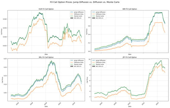
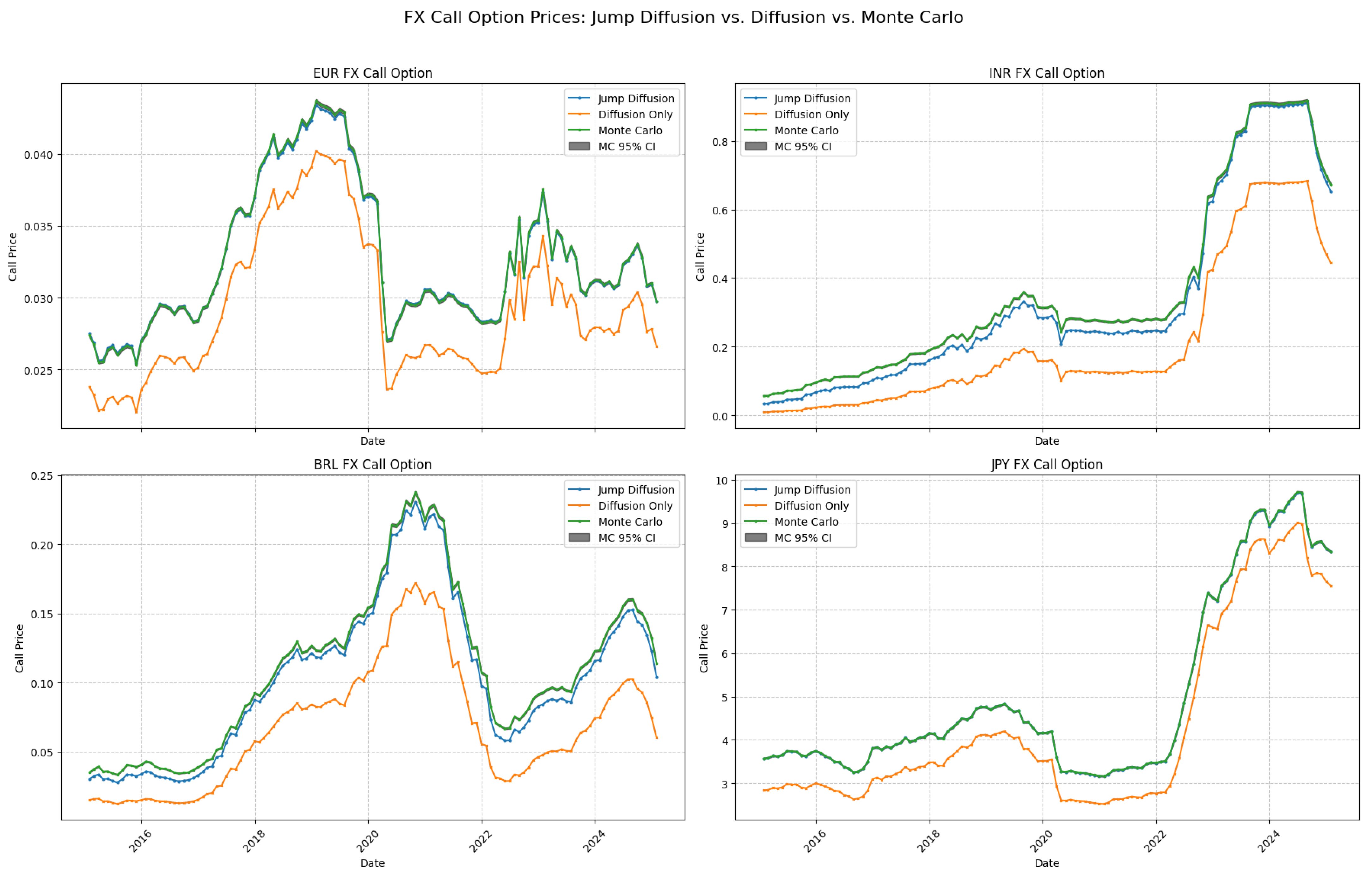
Figure 1 compares the call option prices of the proposed jump-diffusion model $C^{\left(l\right)}(t,T)$ (Equation (6)) and the diffusion-only model against Monte Carlo simulations. Across all dates and currencies, the jump-diffusion model prices closely align with the Monte Carlo simulations. This estimation was performed using 500,000 paths, 150 time steps per unit of maturity, and random seed $=10$, resulting 95% confidence intervals in approximately 0.00021–0.0324 range. For instance, for 31 January 2025, the jump-diffusion price for USD/JPY is $3.561037$ while the Monte Carlo simulation price is $3.563679$, with a $95\%$ confidence interval of [3.5475, 3.5798]. However, the price of the diffusion-only model is $2.833617$, which deviates significantly and indicates a consistent price difference without jumps. While USD/INR and USD/BRL exhibit slightly bigger deviations but are significantly closer to Monte Carlo than the diffusion-only model, USD/EUR and USD/JPY align nearly precisely with MC throughout. No variance reduction techniques were applied in these simulations; hence, the reported standard errors reflect scaling from the large number of simulated paths.

Figure 1. Call option prices on the foreign currency comparison of the proposed jump-diffusion model, the diffusion only model, and Monte Carlo simulation. The x-axis shows the sample period and the y-axis the call price. Each line corresponds to one model, as listed in the legend. Prices are Monte Carlo estimates from 500,000 paths and 150 time steps, with maturity $T=1$ years and the parameters in Table 1.

The metrics for agreement with the Monte Carlo benchmark for call option prices on foreign currency (Figure 1) are reported in Table 8 across all four currency pairs. The proposed jump-diffusion model shows a significant improvement for each pair of currencies. The USD/JPY exchange rate exhibit considerable improvement, with MAPE falling from $15.584\%$ to just $0.130\%$. The proposed model still reduces MAPE to $8.269\%$ and increases $R^2$ to $0.9855$, although USD/BRL exhibits the largest absolute errors under diffusion-only, with MAPE of $44.025\%$, $R^2$ of $0.3919$, which is consistent with its higher jump intensity. USD/INR exhibits a similar trend, with $R^2$ increasing from $0.6517$ to $0.9891$ and MAPE decreasing from $53.148\%$ to $13.967\%$. However, USD/INR still has a larger residual error than EUR and JPY, which is indicative of its previously mentioned jump-dominated variance structure. The $R^2$ varies from $0.39$ to $0.89$, reflecting the exclusion of jumps during unstable market conditions; hence, the diffusion-only model is ineffective at capturing the price of call options in all currency pairs when jumps are present. Thus, the extension of compensated jump components to all three stochastic processes highlights the necessity of considering jumps when pricing FX options.

Table 8. Agreement with the Monte Carlo benchmark metrics for call option prices on foreign currency time series comparison of the proposed jump-diffusion $C^{\left(l\right)}(t,T)$ and diffusion-only models (Figure 1).

Metric	Diffusion-Only Benchmark	Proposed Model	Diffusion-Only Benchmark	Proposed Model
	USD/EUR		USD/INR
RMSE	$3.458\times {10}^{-3}$	$1.290\times {10}^{-4}$	$0.1579$	$0.02798$
MAE	$3.453\times {10}^{-3}$	$1.090\times {10}^{-4}$	$0.1481$	$0.02655$
MAPE (%)	10.782	0.316	53.148	13.967
$R^2$	0.5246	0.9993	0.6517	0.9891
	USD/BRL		USD/JPY
RMSE	$4.405\times {10}^{-2}$	$6.810\times {10}^{-3}$	$0.6851$	$9.350\times {10}^{-3}$
MAE	$4.204\times {10}^{-2}$	$6.666\times {10}^{-3}$	$0.6834$	$6.973\times {10}^{-3}$
MAPE (%)	44.025	8.269	15.584	0.130
$R^2$	0.3919	0.9855	0.8918	0.9999

4. Price of the CAT Bond

In this section, we examine the convergence of the Monte Carlo estimates to the proposed approximation for the CAT bond price with increasing path count. We also present the corresponding approximation error analyses and examine the sensitivity of the CAT bond price to the model parameters.

4.1. Monte Carlo Time Series Simulation

Monte Carlo simulations were performed on the entire sampled time series (2015–2025) for each currency pair. In these simulations, only the exchange and both interest rates were updated at each date. We set the strike as $K=S_0$ (at-the-money strike) for all pairs, so the comparison across currencies isolates the effect of jumps. Other moneyness levels are left for future work. The jump and rate parameters $(\kappa ,\theta ,\sigma ,\lambda ,\beta ,\delta ,\rho )$ are calibrated once throughout the 2015–2025 sample, and remain fixed.

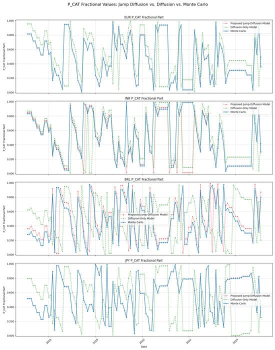
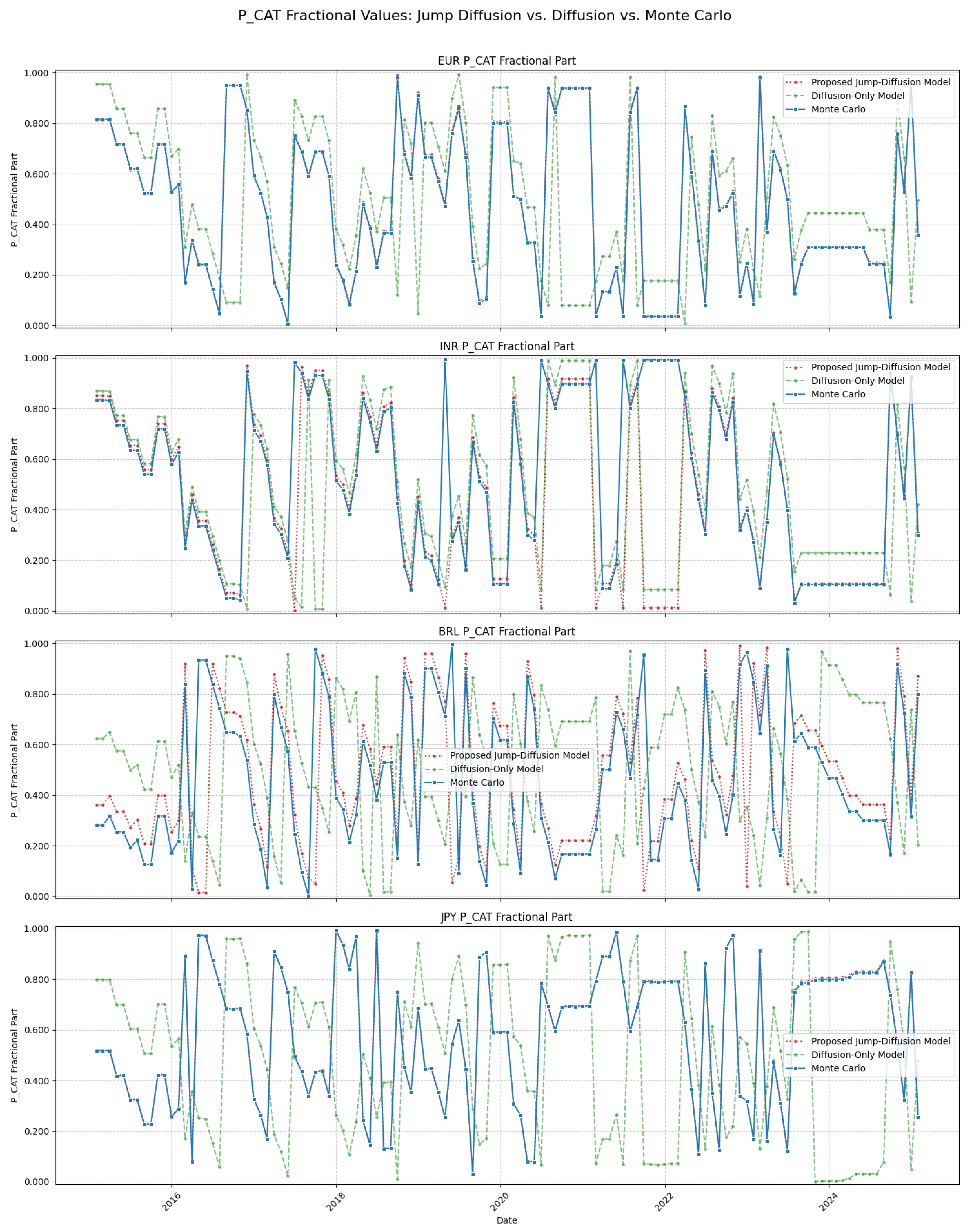
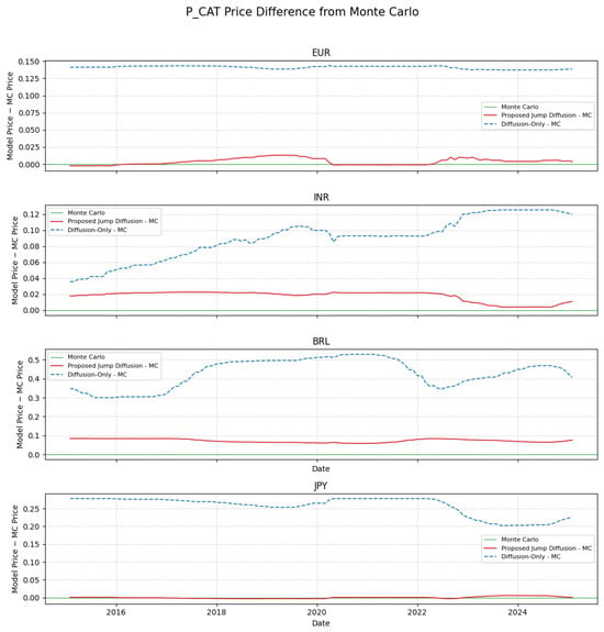
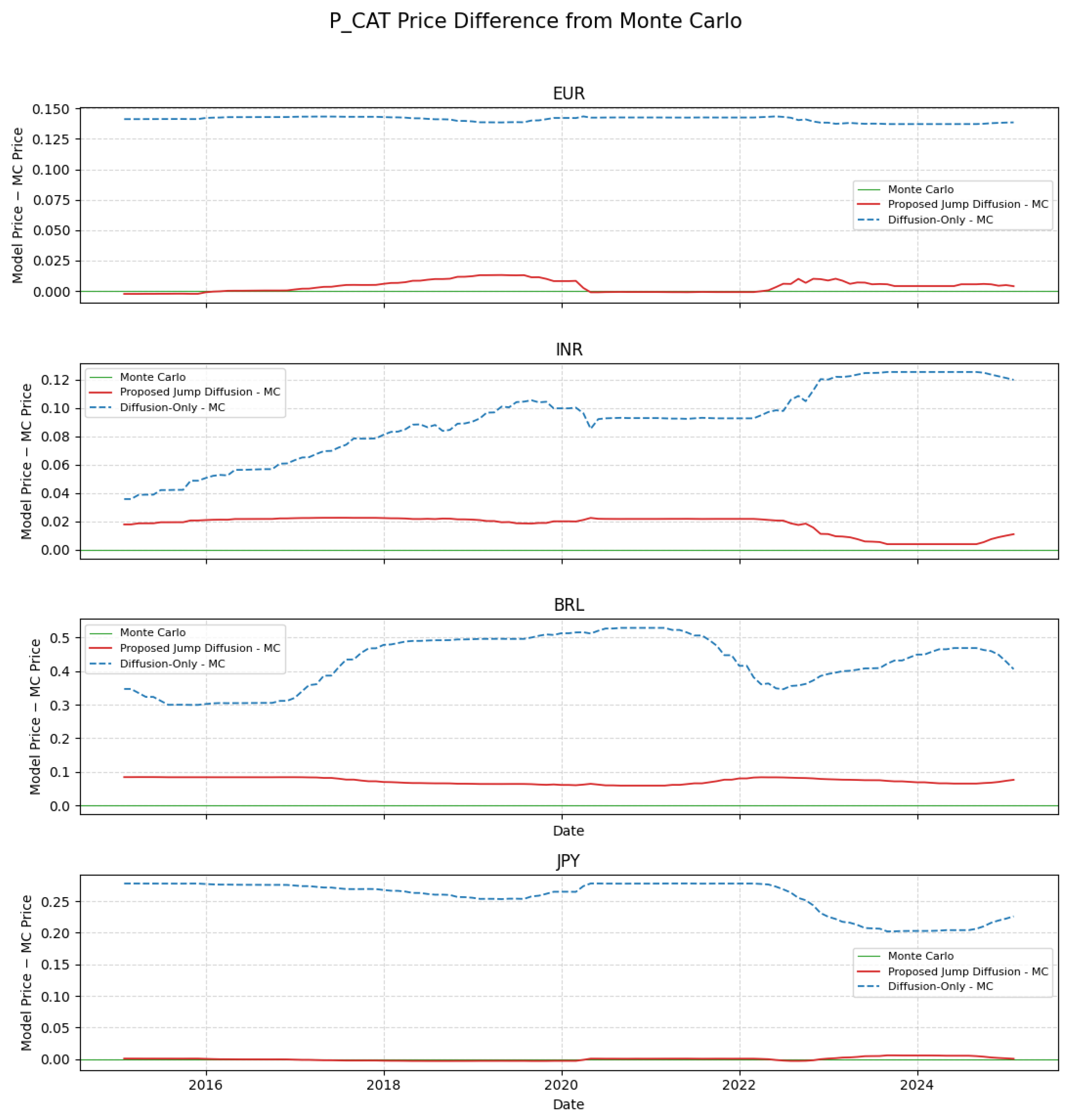
The proposed jump-diffusion approximation $P_{CAT}^{\left(l\right)}(t,T)$ (Theorem 1) and diffusion-only benchmark CAT bond prices were compared to the MC-estimated price at each date for four pairs of currencies, with the results presented in Figure 2. In addition to Figure 2, Figure 3 shows the difference of the proposed and diffusion-only model from Monte Carlo across the sample period. This simulation was performed with 500,000 paths, 150 time steps per unit of maturity, and fixed random seed $=10$. For USD/EUR and USD/JPY, the proposed model $P_{CAT}^{\left(l\right)}(t,T)$ tracks MC nearly exactly in the time series; however, for USD/BRL and USD/INR, the proposed model exhibits some substantial deviation from MC, although it is still consistently closer than the diffusion-only model, which not only deviates further but also frequently does so in the opposite direction.

Figure 2. Comparison of fractional CAT bond prices (defined as $P_{\mathrm{CAT}}-\lfloor P_{\mathrm{CAT}}\rfloor$) for the proposed jump-diffusion, diffusion-only, and Monte Carlo models (2015–2025). The x-axis tracks the sample period, while the y-axis shows the post-decimal fractional price values. Lines represent individual models as labeled in the legend. The estimates utilize 500,000 simulation paths, 150 time steps, maturity $T=1$ year, and the parameters from Table 1.

Figure 3. Pricing deviations from the Monte Carlo simulation for the proposed jump-diffusion ($P_{\mathrm{CAT}}^{JD}-P_{\mathrm{CAT}}^{MC})$ and diffusion-only $(P_{\mathrm{CAT}}^D-P_{\mathrm{CAT}}^{MC}$) models over the sample period 2015–2025. The remaining simulation specifications follow Figure 2.

The corresponding metrics for the agreement with the Monte Carlo benchmark are reported in Table 9. Both models achieve $R^2$ above $0.999$ for all pairs. Nevertheless, the proposed model continuously decreases the error even more: RMSE decreases from $2.597\times {10}^{-1}$ to $3.037\times {10}^{-3}$ for USD/JPY and from $1.389\times {10}^{-1}$ to $5.170\times {10}^{-3}$ for USD/EUR. Due to its greater volatility and jump intensity, USD/BRL exhibits the highest absolute errors under the diffusion-only model (RMSE of $4.321\times {10}^{-1}$), but the proposed model still reduces RMSE to $6.971\times {10}^{-2}$. Among the four pairs, USD/INR exhibits the least amount of relative improvement (RMSE decreases from $9.294\times {10}^{-2}$ to $1.787\times {10}^{-2}$), which is consistent with the wider approximation gap previously observed for the ${\left({\nu }^{\left(l\right)}\right)}^2$ term of USD/INR. Together, these findings indicate that the proposed jump-diffusion extension is in closer agreement with the Monte Carlo benchmark across all four currency pairs, although the magnitude of the improvement varies by currency.

Table 9. Metrics for agreement with the Monte Carlo benchmark for price of CAT bond time series comparison of the proposed jump-diffusion and diffusion-only model against Monte Carlo simulations (Figure 2).

Metric	Diffusion-Only Benchmark	Proposed Model	Diffusion-Only Benchmark	Proposed Model
	USD/EUR		USD/INR
RMSE	$1.389\times {10}^{-1}$	$5.170\times {10}^{-3}$	$9.294\times {10}^{-2}$	$1.787\times {10}^{-2}$
MAE	$1.389\times {10}^{-1}$	$4.359\times {10}^{-3}$	$8.925\times {10}^{-2}$	$1.683\times {10}^{-2}$
MAPE (%)	0.01483	0.00047	0.00956	0.00178
$R^2$	0.99994	0.9999999	0.99997	0.99999
	USD/BRL		USD/JPY
RMSE	$4.321\times {10}^{-1}$	$6.971\times {10}^{-2}$	$2.597\times {10}^{-1}$	$3.037\times {10}^{-3}$
MAE	$4.253\times {10}^{-1}$	$6.913\times {10}^{-2}$	$2.583\times {10}^{-1}$	$2.439\times {10}^{-3}$
MAPE (%)	0.04543	0.00738	0.02755	0.00026
$R^2$	0.99938	0.99998	0.999788	0.9999994

USD/INR has the weakest call option fit in Table 8 but a low CAT bond MAPE in Table 9. The call price enters $P_{CAT}^{\left(l\right)}$ through the term $V\omega \mathbb{Q}(\eta \le T)C^{\left(l\right)}/K^{\left(l\right)}$. With $\omega =0.9$ and $\mathbb{Q}(\eta \le T)=0.05$, the call error is scaled by a factor of $0.045$ in its contribution to the bond price. The remaining component of $P_{CAT}^{\left(l\right)}$ depends on $P_d(t,T)$, which is identical across all pairs. Larger values of $\omega$ or $\mathbb{Q}(\eta \le T)$ would increase the contribution of the call error to $P_{CAT}^{\left(l\right)}$.

4.2. Monte Carlo Convergence

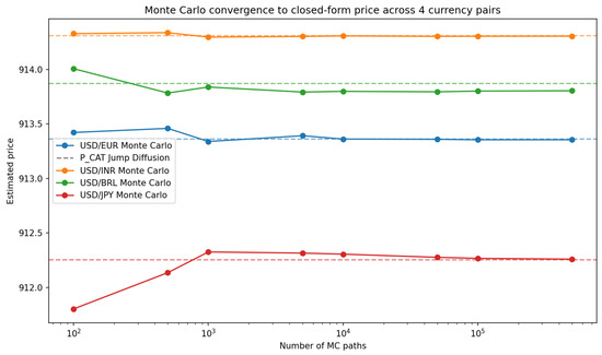
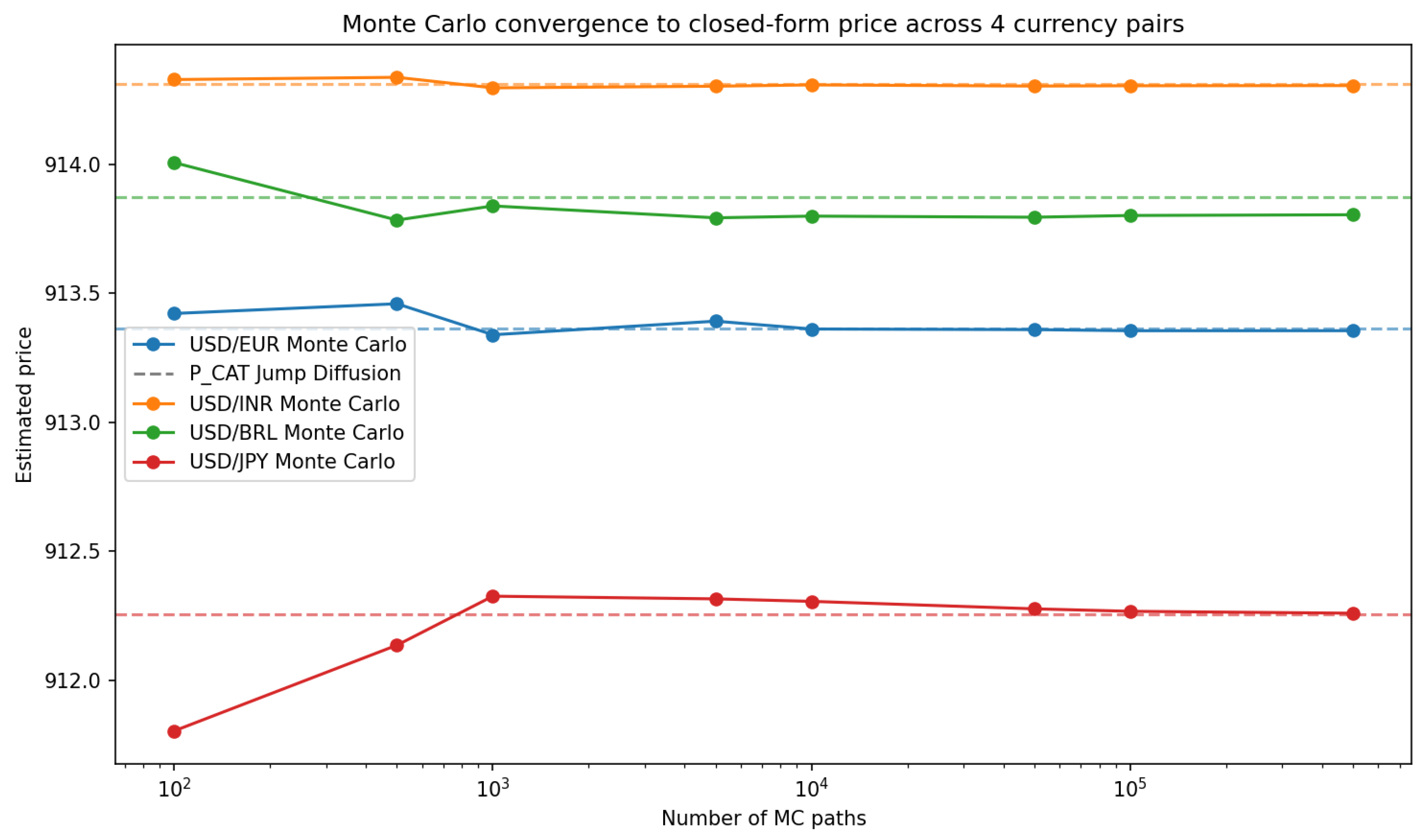
To evaluate the numerical stability of the proposed price of the CAT bond $P_{CAT}^{\left(l\right)}(t,T)$ (Theorem 1), the Monte Carlo estimate was monitored with an increasing number of simulation paths. The MC estimate stabilizes around the proposed $P_{CAT}^{\left(l\right)}(t,T)$ in Figure 4, with final percentage differences of USD/EUR $(0.00075\%)$, USD/INR $(0.00080\%)$, USD/BRL $(0.00746\%)$, and USD/JPY $(0.00050\%)$. This pattern is statistically confirmed by Table 10: USD/INR exhibits the tightest convergence (RMSE $\approx 0.013$, MAPE $\approx 0.0013\%$), while USD/JPY exhibits the highest variation, though this is still economically negligible when compared to the face value of 1000. The MC estimator converges to the closed-form price with MAPE of $0.0060\%$ when pooled across all four pairs, demonstrating the numerical consistency of the proposed $P_{CAT}^{\left(l\right)}(t,T)$ approximation with Monte Carlo.

Figure 4. Convergence of the CAT bond price of Monte Carlo simulation and the proposed price for USD/EUR, USD/INR, USD/BRL and USD/JPY. The x-axis shows the number of simulated paths (up to 500,000 and 150 time steps) and the y-axis shows the CAT bond price per 1000 face value in USD. Each color shows one currency pair, with the dashed line marking the respective proposed price. Parameters are same as in Table 1, with $Q=0.05$ and seed 10.

Table 10. RMSE, MAE, and MAPE of the Monte Carlo estimate relative to its largest path (Figure 4) for the proposed $P_{CAT}^{\left(l\right)}(t,T)$ price.

Currency	RMSE	MAE	MAPE %
USD/BRL	0.082574	0.078428	0.008582
USD/EUR	0.042712	0.028357	0.003105
USD/INR	0.013451	0.011970	0.001309
USD/JPY	0.169502	0.098714	0.010821
ALL (pooled)	0.096895	0.054367	0.005954

The Monte Carlo price is shown in Table 11 with its standard error, $95\%$ confidence interval, and error versus the proposed model for four independent seeds for $N=500,000$ paths. The results in Table 10 are not sensitive to the choice of a random seed, as the estimates are consistent between seeds and the variations only reflect the results after the third decimal point. The sign of the approximation error is consistent within every currency across all seeds. USD/BRL has the highest calibrated jump intensity and jump size in both foreign rate and exchange rate $({\lambda }_f=1.3,{\delta }_S=0.083)$. Since the proposed approximation matches the total variance, this is consistent with the negative error observed for this pair in Table 11.

Table 11. CAT bond price results for Monte Carlo and the proposed model by currency and independent seed.

Seed	MC Price	Proposed Model Price	MC S.E.	95% CI Lower	95% CI Upper	Error vs. Proposed	MC Time (s)	Analytical Time (s)
USD/EUR
10	913.354499	913.059111	$5.38310310\times {10}^{-5}$	913.349914	913.359084	0.295388	28.203847	0.000400820
3	913.356606	913.059111	$5.37103958\times {10}^{-5}$	913.352032	913.361181	0.297495	28.068938	0.000400820
20	913.357261	913.059111	$5.38542911\times {10}^{-5}$	913.352674	913.361847	0.298150	27.900769	0.000400820
42	913.357903	913.059111	$5.37403490\times {10}^{-5}$	913.353326	913.362480	0.298792	27.822306	0.000400820
USD/INR
10	914.304190	914.052878	$2.19773687\times {10}^{-3}$	914.301943	914.306437	0.251312	27.552404	0.000386090
3	914.301266	914.052878	$2.21590846\times {10}^{-3}$	914.299001	914.303532	0.248388	27.638833	0.000386090
20	914.301320	914.052878	$2.21336460\times {10}^{-3}$	914.299057	914.303583	0.248442	27.629636	0.000386090
42	914.302480	914.052878	$2.20142022\times {10}^{-3}$	914.300229	914.304731	0.249602	27.017562	0.000386090
USD/BRL
10	913.803710	914.643781	$4.48839596\times {10}^{-4}$	913.797124	913.810296	−0.840071	27.410957	0.000672794
3	913.797983	914.643781	$4.49684827\times {10}^{-4}$	913.791385	913.804582	−0.845798	26.879772	0.000672794
20	913.797453	914.643781	$4.50688712\times {10}^{-4}$	913.790840	913.804066	−0.846328	27.344691	0.000672794
42	913.794990	914.643781	$4.54022933\times {10}^{-4}$	913.788328	913.801652	−0.848791	27.348694	0.000672794
USD/JPY
10	912.259809	911.379803	$1.34721611\times {10}^{-2}$	912.252215	912.267402	0.880006	27.334174	0.000368999
3	912.260060	911.379803	$1.34594429\times {10}^{-2}$	912.252474	912.267647	0.880258	28.125179	0.000368999
20	912.264268	911.379803	$1.34708519\times {10}^{-2}$	912.256676	912.271861	0.884466	27.652799	0.000368999
42	912.257028	911.379803	$1.34673524\times {10}^{-2}$	912.249437	912.264619	0.877225	27.626975	0.000368999

4.3. Parameter Sensitivity

For all four currency pairs, Table 12 shows $P_{CAT}^{\left(l\right)}(t,T)$ under the proposed jump-diffusion and diffusion-only models across five levels of catastrophe event probability: $\mathbb{Q}(\eta \le T)=0.01,0.05,0.10,$$0.20$, and $0.30$. In accordance with the linear dependence of $\mathbb{Q}(\eta \le T)$ on the CAT bond price, the difference between the two models increases linearly with $\mathbb{Q}(\eta \le T)$. The difference between USD and EUR increases from $0.0269$ at $\mathbb{Q}(\eta \le T)=0.01$ to $0.8068$ at $\mathbb{Q}(\eta \le T)=0.30$, which is almost thirty times greater, corresponding to the same increase in $\mathbb{Q}(\eta \le T)$ itself. All currency pairs exhibit this linear scaling. USD/EUR and USD/INR exhibit the least divergence throughout, with the gap to INR continuously slightly below that to EUR at low $\mathbb{Q}(\eta \le T)$, but converging closer at higher $\mathbb{Q}(\eta \le T)$ (0.6535 for INR versus 0.8068 for EUR at $\mathbb{Q}(\eta \le T)=0.30$). USD/JPY has the second-largest gap (1.3518 at $\mathbb{Q}(\eta \le T)=0.30$). As per the higher jump intensity and volatility calibration, USD/BRL exhibits the biggest gap at all levels of $\mathbb{Q}(\eta \le T)$. At $\mathbb{Q}(\eta <T)=0.30$, the gap to BRL reaches $1.9782$, which is the greatest of the four pairs and about $2.5$ times the gap to EUR of $0.8068$.

Table 12. Sensitivity of CAT bond price to the catastrophe trigger probability $\mathbb{Q}(\eta \le T)$.

Currency	Proposed Model	Diffusion-Only Benchmark	Gap	Proposed Model	Diffusion-Only Benchmark	Gap
	$\mathbb{Q}(\eta \le T)=0.01$			$\mathbb{Q}(\eta \le T)=0.05$
USD/EUR	948.9001	948.8732	0.0269	913.4958	913.3614	0.1345
USD/INR	949.0850	949.0632	0.0218	914.4204	914.3115	0.1089
USD/BRL	949.0412	948.9753	0.0659	914.2016	913.8719	0.3297
USD/JPY	948.6970	948.6519	0.0451	912.4806	912.2553	0.2253
	$\mathbb{Q}(\eta \le T)=0.1$			$\mathbb{Q}(\eta \le T)=0.2$
USD/EUR	869.2406	868.9716	0.2689	780.7300	780.1922	0.5379
USD/INR	871.0897	870.8718	0.2178	784.4282	783.9926	0.4356
USD/BRL	870.6521	869.9928	0.6594	783.5532	782.2344	1.3188
USD/JPY	867.2100	866.7594	0.4506	776.6689	775.7678	0.9012
	$\mathbb{Q}(\eta \le T)=0.3$
USD/EUR	692.2195	691.4127	0.8068
USD/INR	697.7668	697.1133	0.6535
USD/BRL	696.4542	694.4761	1.9782
USD/JPY	686.1279	684.7761	1.3518

5. Discussion

Table 6 and Table 7 implement the moment-matched lognormal approximation for the conditional variance ${\left({\nu }^{\left(l\right)}\right)}^2$ and compare its error to the Monte Carlo benchmark. For feasibility reasons, Section 3 uses this approximation instead of the explicit characteristic function from Section 2. These comparisons evaluate the approximation against simulated prices under the proposed model, not against market prices of CAT bonds. We use a jump-diffusion model rather than Bayesian or machine learning approaches [3] in order to maintain a direct link to the CAT bond pricing structure of [8].

The jump extension gives the largest accuracy gains for currency pairs with higher jump activity, such as USD/BRL, and gives little advantage for low-jump pairs such as USD/JPY at short maturities; therefore, it is most useful to issuers and investors who price and hedge CAT bonds tied to currencies with higher jump intensity, such as BRL. A sponsor of a foreign currency CAT bond faces both the catastrophe trigger and exchange rate movements. The pricing framework shows the separate contributions of each to the bond price, which can guide hedging of the exchange rate leg independently of catastrophes.

It is important to note that the results rely on simplified assumptions. The face value V, loss severity $\omega$, and trigger probability $\mathbb{Q}(\eta \le T)$ are fixed exogenously from [8] to allow for a direct comparison with their results, rather than being estimated from data (Section 3.1). The payoff is simple: a single trigger and a fixed proportional loss allows the holder to keep the face value or lose a fixed fraction of it. Notably, many traded CAT bonds use indemnity or industry loss triggers, layered losses, and coupons, while our parametric-type index ignores basis risk. Jump sizes are normal and independent across the four currency pairs, which misses simultaneous jumps during global crises. The calibration sample (January 2015 to January 2025) includes the COVID-19 pandemic period, when exchange rate moves were unusually large; thus, the estimated jump intensity and jump size parameters may be inflated. The sensitivity analysis covers $\mathbb{Q}(\eta \le T)$. The joint effect of the jump parameters on $P_{CAT}^{\left(l\right)}(t,T)$ is visible in the jump-diffusion versus diffusion-only comparison, but the separate effects of the jump intensity, jump standard deviation, and correlation parameters were not isolated.

As in [8], Assumption 2 takes the catastrophe trigger $\eta$ independent of interest rates and exchange rates, which is done for tractability; however, this may fail across currencies and for very large events. A major hurricane could weaken BRL more than JPY, and mega-events such as the 2011 Tohoku earthquake and tsunami can move both interest rates and exchange rates. The effect on the currency component is direct: the price formula multiplies $\mathbb{Q}(\eta \le T)$ by $C^{\left(l\right)}(t,T)$, which holds only under independence; if a catastrophe that triggers the bond also depreciates the foreign currency, then the call is worth less in the triggered states than $C^{\left(l\right)}(t,T)$, and the formula will overstate the loss. Under independence, the call component and bond price would then be mis-stated. A natural extension lets catastrophe jumps be correlated with exchange rate jumps, for instance through a common Poisson shock. The conditional expectation then no longer factors, and the price is computed jointly by simulation.

Future work includes this correlated extension with a quantitative sensitivity analysis, a parameter-by-parameter sensitivity analysis of the jump parameters, layered loss structures, coupon-paying bonds, validation against market CAT bond prices, and a comparison with Bayesian and machine learning methods.

6. Conclusions

This paper prices CAT bonds on four currency pairs (USD/EUR, USD/INR, USD/BRL, USD/JPY) using a jump-diffusion model for the spot exchange rate and both the domestic and foreign short rates. Under the assumption that the catastrophe trigger is independent of financial markets, the CAT bond price combines the domestic and foreign zero-coupon bond prices with a moment-matched lognormal call option on the foreign currency. Parameters are calibrated for each pair on monthly data from January 2015 to January 2025.

The numerical analysis compares the bond prices and the conditional variance against Monte Carlo over several maturities, both without jumps $(\lambda =0)$ and with jumps $(\lambda >0)$. It also covers the time series for the FX call option and the CAT bond price, a sensitivity analysis of the trigger probability, and Monte Carlo convergence checks across path counts and random seeds. The approximate prices are compared with Monte Carlo prices generated under the identical jump-diffusion dynamics. Relative to the diffusion-only model, the jump-diffusion approximation reproduces the simulated CAT bond prices more closely for every pair. The CAT bond MAPE falls from 0.0276% to 0.0003% for JPY and from 0.0148% to 0.0005% for EUR. For the call options, the MAPE falls from 15.6% to 0.1% for JPY and from 53.1% to 14% for INR. These comparisons are internal to the assumed dynamics; validation against real market CAT bond prices is left for future work.

References

- Merton, R.C. Option Pricing When Underlying Stock Returns Are Continuous. J. Financ. Econ. 1976, 3, 125–144. [Google Scholar] [CrossRef] [Scilit]
- Vaugirard, V.E. Pricing catastrophe bonds by an arbitrage approach. Q. Rev. Econ. Financ. 2003, 43, 119–132. [Google Scholar] [CrossRef] [Scilit]
- Domfeh, D.; Chatterjee, A.; Dixon, M. A Bayesian valuation framework for catastrophe bonds. J. R. Stat. Soc. Ser. C Appl. Stat. 2024, 73, 1389–1410. [Google Scholar] [CrossRef] [Scilit]
- Gagliardini, P.; Gouriéroux, C.; Trojani, F. Robust risk pricing with applications to catastrophe bonds. J. Financ. Econom. 2011, 9, 471–502. [Google Scholar]
- Cox, S.H.; Pedersen, H.W. Catastrophe risk bonds. N. Am. Actuar. J. 2000, 4, 56–82. [Google Scholar] [CrossRef] [Scilit]
- Hilliard, J.E.; Madura, J.; Tucker, A.L. Currency option pricing with stochastic domestic and foreign interest rates. J. Financ. Quant. Anal. 1991, 26, 139–151. [Google Scholar] [CrossRef] [Scilit]
- Nowak, P.; Romaniuk, M. Pricing and simulations of catastrophe bonds. Insur. Math. Econ. 2013, 52, 18–28. [Google Scholar] [CrossRef] [Scilit]
- Lai, V.S.; Parcollet, M.; Lamond, B.F. The valuation of catastrophe bonds with exposure to currency exchange risk. Int. Rev. Financ. Anal. 2014, 33, 243–252. [Google Scholar] [CrossRef] [Scilit]
- Bates, D.S. Jumps and Stochastic Volatility: Exchange Rate Processes Implicit in Deutsche Mark Options. Rev. Financ. Stud. 1996, 9, 69–107. [Google Scholar] [CrossRef] [Scilit]
- Nehra, R.; SenGupta, I. The valuation of catastrophe bonds under domestic and foreign interest rates with jumps. 2026; submitted.
- Cartea, A.; Figueroa, M.G. Pricing in electricity markets: A mean reverting jump diffusion model with seasonality. Appl. Math. Financ. 2005, 4, 313–335. [Google Scholar] [CrossRef] [Scilit]
- Sahalia, Y.A. Disentangling diffusion from jumps. J. Financ. Econ. 2004, 74, 487–528. [Google Scholar] [CrossRef] [Scilit]
- Härdle, W.K.; Cabrera, B.L. Calibrating CAT bonds for Mexican earthquakes. J. Risk Insur. 2010, 77, 625–650. [Google Scholar] [CrossRef] [Scilit]
- Poncet, P.; Vaugirard, V.E. The valuation of nature-linked bonds with exchange rate risk. J. Econ. Financ. 2001, 25, 293–307. [Google Scholar] [CrossRef] [Scilit]
- Shreve, S.E. Stochastic Calculus for Finance II Continuous-Time Models; Springer: Berlin/Heidelberg, Germany, 2004. [Google Scholar]
- Harris, C.R.; Millman, K.J.; Van Der Walt, S.J.; Gommers, R.; Virtanen, P.; Cournapeau, D.; Wieser, E.; Taylor, J.; Berg, S.; Smith, N.J.; et al. Array programming with NumPy. Nature 2020, 585, 357–362. [Google Scholar] [CrossRef] [Scilit] [PubMed]
- Paszke, A.; Gross, S.; Massa, F.; Lerer, A.; Bradbury, J.; Chanan, G.; Killeen, T.; Lin, Z.; Gimelshein, N.; Antiga, L.; et al. PyTorch: An imperative style, high-performance deep learning library. Adv. Neural Inf. Process. Syst. 2019, 32, 8024–8035. [Google Scholar]
- Virtanen, P.; Gommers, R.; Oliphant, T.E.; Haberland, M.; Reddy, T.; Cournapeau, D.; Burovski, E.; Peterson, P.; Weckesser, W.; Bright, J.; et al. SciPy 1.0: Fundamental algorithms for scientific computing in Python. Nat. Methods 2020, 17, 261–272. [Google Scholar] [CrossRef] [Scilit] [PubMed]
- Chan, K.C.; Karoyli, G.A.; Longstaff, F.A.; Sanders, A.B. An empirical comparison of alternative models of the short-term interest rate. J. Financ. 1992, 47, 1209–1227. [Google Scholar] [CrossRef] [Scilit]
Disclaimer/Publisher’s Note: The statements, opinions and data contained in all publications are solely those of the individual author(s) and contributor(s) and not of MDPI and/or the editor(s). MDPI and/or the editor(s) disclaim responsibility for any injury to people or property resulting from any ideas, methods, instructions or products referred to in the content. |
© 2026 by the authors. Licensee MDPI, Basel, Switzerland. This article is an open access article distributed under the terms and conditions of the Creative Commons Attribution (CC BY) license.