


Abstract
In the present work, we study combined m-consecutive--out-of-n and consecutive -out-of-n reliability systems under imperfect cold standby redundancy. The proposed framework extends the ordinary perfect standby assumption by allowing the activation of the spare system to be successful with a given coverage probability. The system-level redundancy policy is considered, while the classical perfect cold standby model is obtained as a special case. Exact reliability representations for the resulting structures are discussed through signature-based arguments. In particular, expressions for the reliability function, the Mean Time to Failure and the Mean Residual Lifetime are provided. Special emphasis is also placed on statistical inference under right-censored lifetime data. A numerical study is carried out to illustrate the effect of imperfect coverage, censoring, and design parameters on the performance of the proposed reliability schemes.
1. Introduction
In the field of statistical reliability modeling, consecutive-type systems have been widely used for the representation and analysis of engineering structures whose performance is strongly affected by the relative ordering of non-working components. Such systems arise naturally in several practical settings, including telecommunication networks, pipeline systems, integrated circuits, sensor arrays, transportation systems, and quality-control schemes. The classical consecutive-k-out-of-n system consists of n linearly or circularly ordered components and fails if and only if at least k consecutive components fail (see, e.g., [1,2,3]). Due to its simple structure and its wide applicability, this model has attracted considerable research interest and has motivated several generalizations during recent decades. For instance, one may refer to the r-within-consecutive k-out-of-n: F system, whose failure occurs if and only if there exist k consecutive components which include among them at least r failed ones. The latter structure was established by [4] and has been further studied by many authors (see, e.g., [5,6]). In addition, the so-called m-consecutive-k-out-of-n: F system seems to be a natural generalization of the classical m-out-of-n: F system and the consecutive-k-out-of-n: F system; it consists of n linearly ordered components such that the structure fails if and only if there are at least m non-overlapping runs of k consecutive failed components. This system was first introduced by [7] and since then it has attracted some research attention (see, e.g., [8,9]).
Among the most important extensions of the ordinary consecutive-k-out-of-n system are reliability structures operating under more than one failure criterion. Such systems are particularly useful when the overall failure of a structure cannot be described by a single type of component failure pattern. For instance, a system may stop functioning either because a sufficiently long run of consecutive failed components appears or because several smaller non-overlapping ones occur across the system. In this direction, combined consecutive-type structures with two common failure criteria provide a flexible framework for modeling complex engineering systems (see, e.g., [10,11,12]).
The present paper focuses on the combined -consecutive--out-of- and consecutive -out-of- structure () hereafter). The system consists of linearly ordered components and fails if and only if there exist at least consecutive failed components or at least non-overlapping runs of consecutive failed components (see, e.g., [13,14]). The aforementioned reliability scheme includes several well-known models as special cases and is suitable for applications in which both local concentration of failures and repeated clustered failures may cause the breakdown of the system.
A common way to improve the performance of reliability systems is the implementation of cold standby redundancy, which may be applied either at the system level, by activating a complete spare system after failure of the primary one, or at the component level, by assigning a spare unit to each primary component (see, e.g., [15,16,17,18]). The relative efficiency of these two policies depends on the system design, the component lifetime distribution, and the reliability criterion under consideration.
Most works on cold standby redundancy assume perfect switching, namely that the spare unit is activated successfully whenever the primary system or component fails. In practice, however, successful activation may be hindered by switching failures, delayed fault detection, or the unavailability of the spare unit. Therefore, the assumption of imperfect standby coverage provides a more realistic framework for reliability evaluation.
In system-level standby redundancy, the entire spare system remains inactive and is activated only after the failure of the primary system. Therefore, the standby mechanism operates at the level of the whole structure. In contrast, under component-level standby redundancy, each primary component is equipped with its own spare unit and the activation mechanism operates separately for each component. The present work focuses on the system-level policy, where the coverage probability describes the successful activation of the spare system as a whole.
In the present paper, we study the reliability structure under imperfect cold standby redundancy, focusing mainly on the system-level policy. We assume that, upon failure of the primary system, the spare system is activated successfully with coverage probability , .
The first objective of the work is to derive reliability representations for the proposed model. By the aid of the signature vector of the underlying structure, expressions for the survival function, the Mean Time to Failure, and the Mean Residual Lifetime are obtained. On the other hand, a likelihood-based inference procedure under right-censored lifetime data is also developed. The component lifetime distribution is assumed to belong to a parametric family, while both its parameters and the coverage probability are treated as unknown. The resulting censored-data likelihood is used to estimate the model parameters, which are then inserted into the derived reliability expressions to estimate the reliability characteristics of the underlying structure. For a survey on basic models of censoring mechanisms with a focus on lifetime data, failure data, and reliability applications, the interested reader is referred to [19].
Despite the extensive literature on consecutive-type systems and standby redundancy, statistical inference for combined consecutive-type systems under imperfect cold standby coverage has received limited attention. In many practical applications, such as engineering devices, monitoring systems, transportation systems, and communication networks, the exact system failure time may not always be fully observed because units can be removed from observation, inspections may terminate before failure, or data collection may stop at a predetermined time. Therefore, right-censored lifetime data are frequently encountered in reliability applications. At the same time, the activation of a standby system may not be perfect. The spare system may fail to activate due to switching failures, coverage failures or imperfect fault detection. These practical issues motivate the need for an inferential framework that combines consecutive-type system structures, imperfect standby activation, and censored lifetime observations.
The main research problem addressed in this paper is the estimation of the reliability characteristics of a combined -consecutive--out-of- and consecutive -out-of- structure when the system is equipped with an imperfect cold standby unit and the observed data are subject to independent right censoring.
The rest of the paper is organized as follows. Section 2 introduces the structure with imperfect cold standby redundancy at the system level. Section 3 provides the main reliability results, including formulae for the survival function, the Mean Time to Failure, and the Mean Residual Lifetime. Section 4 presents the likelihood-based inference procedure under right-censored data, wherein the corresponding plug-in estimation of the main reliability characteristics is also described. Section 5 provides some numerical evidence for illustrating the effect of the coverage probability, the censoring mechanism and the design parameters on the performance of the resulting system. Section 6 provides a practical application of the proposed reliability scheme, while Section 7 summarizes the main conclusions and outlines possible directions for future research.
2. The System-Level Imperfect Standby Framework
In the present section, we introduce the general framework of the combined -consecutive--out-of-: F and consecutive -out-of-: F structure under imperfect cold standby redundancy at the system level.
The structure, which consists of linearly ordered components, fails if and only if at least one of the following two failure criteria is satisfied:
- There exist at least consecutive failed components;
- There exist at least m non-overlapping runs of k consecutive failed components.
For instance, consider the design (6,2,2,3). The system fails if either three consecutive components fail, or if there are two non-overlapping runs of two consecutive failed components. Therefore, the failure pattern 0 1 1 1 0 0 causes system failure because it contains three consecutive failed components. Also, the configuration 1 1 0 1 1 0 causes failure because it contains two non-overlapping runs of length 2. In contrast, the configuration 1 1 0 1 0 0 does not cause failure, since it contains only one run of two consecutive failed components and no run of three consecutive failed components.
Let denote the lifetimes of the components of the primary system and let correspond to the respective ones of the components of the spare system. Unless otherwise stated, all component lifetimes are assumed to be independent and identically distributed with common continuous distribution function , where is an unknown parameter vector.
In what follows, denotes the lifetime function induced by the failure criterion of the ordinary structure. More precisely, for any vector of component lifetimes , the quantity is defined as the first time at which the set of failed components satisfies at least one of the two failure criteria of the system, namely the occurrence of at least consecutive failed components or the occurrence of at least non-overlapping runs of consecutive failed ones.
We next denote by and the lifetime of the primary system and the spare one respectively. The random variables , are assumed to be identically distributed and mutually independent.
Under perfect cold standby redundancy at the system level, the spare system is activated whenever the primary system fails. However, throughout the lines of the present work, the activation of the spare system is not assumed to be perfect. More specifically, let be a Bernoulli random variable such that
where . The parameter represents the coverage probability, namely the probability that the spare system is successfully activated after the failure of the primary system. The random variable is assumed to be independent of the component lifetimes of both the primary and the spare systems. Throughout the paper, the resulting structure, namely the structure with imperfect cold standby redundancy at the system level, shall be denoted by .
The lifetime of the structure is then defined as
or equivalently
Since is a Bernoulli random variable independent of and , the lifetime can be interpreted conditionally on the value of . If , the activation of the spare system is successful and the total lifetime is . If , the activation fails and the system lifetime remains equal to . Therefore, conditioning on yields the mixed representation in (3), with probabilities and .
Thus, if the spare system is successfully activated, the total lifetime of the redundant structure is the sum of the lifetimes of the primary and spare systems. On the other hand, if the activation attempt fails, the overall system fails at the failure time of the primary structure. It is straightforward that the special case yields the ordinary system without effective standby redundancy (see, e.g., [8]), whereas corresponds to the classical perfect cold standby model (see [12]).
For illustration purposes, consider the structure . The particular system consists of eight linearly ordered components and fails if and only if either four consecutive components fail or three non-overlapping pairs of consecutive failures occur. Suppose that a spare system is available at the system level. At the beginning of operation, the primary system is active, whereas the spare system remains inactive. When the primary system reaches one of the two failure criteria, an activation attempt for the spare system is made. With probability , the spare system is successfully activated and starts operating as a new system. With probability , the activation fails and the overall structure stops operating immediately at the failure time of the primary system.
This example illustrates the main difference between perfect and imperfect cold standby redundancy. In the perfect case, the failure of the primary system always leads to the operation of the spare system. In the imperfect case, the lifetime of the overall structure also depends on the success or failure of the activation mechanism, as described by the coverage probability .
3. Reliability Characteristics of the Proposed
Throughout the next lines, we investigate some reliability characteristics of the structure, which was introduced in the previous section. Let
denote the signature vector of the ordinary system, where
while are the order statistics which correspond to the lifetimes of its components. To be clearer, the i-th coordinate defined in (4) provides the value of the portion , where corresponds to the amount of the specific orderings of the , whose realization means that when the i-th component fails, then the whole system stops its operation (see, e.g., [13]).
The signature vector can be computed by enumerating all possible failed component subsets of size , for . Let denote the probability that the system is still functioning after exactly components have failed, under the assumption that all failure orders are equally likely. Then and , and the i-th signature component is obtained as . For the combined consecutive-type structure, is computed by checking, for each subset of failed positions, whether at least one of the two failure criteria is satisfied.
If and correspond to the common distribution function and reliability function of the component lifetimes respectively, the reliability function of the ordinary system lifetime can be expressed as (see, e.g., [12])
Equation (5) follows from the standard signature representation of coherent systems with independent and identically distributed component lifetimes. Indeed, it is well-known that the system reliability can be described as a weighted mixture of order statistic reliabilities, with weights (see, e.g., [13]).
Proposition 1 offers an exact signature-based representation of the reliability function of the proposed structure. Kindly note that the term “exact” is used in the sense that the reliability expressions are derived directly from the system signature and the probabilistic standby representation , without simulation approximation of the system structure. In general, some integrals appearing in these expressions may need to be evaluated numerically, depending on the component lifetime distribution.
Proposition 1.
The reliability function of the structure is given by
where
Proof.
(i) Recalling that is distributed as a Bernoulli random variable, we next consider the lifetime defined in (3) and the following holds true:
Since
and , are identically distributed, we may write
Combining the relations (9)–(11), the desired expression is readily deduced.
(ii) Since , are independent and identically distributed, we observe that
Conditioning on the value of , we deduce that
and Formula (12) can be rewritten as
Since has the same distribution as , we can state that
and therefore, the following formula is straightforward
Substituting the last expression into the mixture representation (6), the result we are chasing for is effortlessly concluded.
□
It is worth mentioning that the two forms of the reliability function in Proposition 1 serve different purposes. More precisely, the mixture form given in (6) focuses on the probabilistic interpretation of the imperfect standby mechanism, while the other one seems to be useful for numerical evaluation and likelihood-based inference.
Proposition 2 offers a signature-based representation of the Mean Time to Failure of the proposed structure.
Proposition 2.
The Mean Time to Failure of the structure is given by
Proof.
Considering the definition of (see Equation (3)), we observe that
Note that (15) practically expresses the Mean Time to Failure of the resulting system. Since and are independent random variables, it is straightforward that
Given that and are assumed to be identically distributed, we substitute expression (16) in (15) and the following holds true
Recalling the following well-known identity
and the signature-based representation of the corresponding reliability function (see, Equation (5)), we deduce that
The desired result is readily obtained by substituting the last expression in (17). □
Proposition 3 provides an integral expression for determining the Mean Residual Lifetime of the underlying reliability structure with imperfect cold standby redundancy at the system level.
Proposition 3.
The Mean Residual Lifetime of the structure is given by
where corresponds to the probability density function of .
Proof.
Let us assume that . By definition, the Mean Residual Lifetime of at time is given by
Therefore
Since is a non-negative absolutely continuous random variable, we have
where denotes the probability density function of . Applying integration by parts, we obtain
where . Hence
Since , it follows that and therefore
Using Proposition 1, the reliability function of the system-level imperfect standby structure is
Substituting this expression into the previous formula gives
This completes the proof.
□
4. Likelihood-Based Inference Under Right Censoring
In this section, we develop a likelihood-based inference procedure for the structure with imperfect cold standby redundancy at the system level. As it is easily observed, the reliability characteristics derived in the previous section depend on the component lifetime parameter vector and on the coverage probability . In practice, these parameters are almost always unknown and must be estimated from lifetime data.
Let us first denote by the lifetime of the -th observed system, where all systems are assumed to have the same design , the same component lifetime distribution , and the same coverage probability . Due to right censoring, the exact system’s lifetime is not necessarily observed for every replication. Instead, for the -th tested system, we observe
and
where corresponds to the censoring time and is simply the failure indicator. More precisely, coincides with the fact that the failure time of the system is observed, whereas expresses the scenario that the system lifetime is right-censored at time. Note that the censoring mechanism is assumed to be independent of the systems’ lifetimes. If we consider once again the reliability function and the corresponding probability density function for the proposed structure, we are ready to state the following proposition, which offers an explicit expression for determining the censored-data likelihood function for the design parameters of the resulting system. In simple words, the censoring scheme considered within this work is independent random right censoring. The censoring times are assumed to be independent of the system lifetimes . Therefore, the censoring mechanism considered here is not a Type-I, Type-II, or hybrid censoring scheme, but an independent random right censoring scheme. On the other hand, the censoring times that appeared in the numerical study are generated independently from an exponential distribution , where the censoring rate is calibrated in order to obtain the desired nominal censoring proportion.
Although likelihood construction under independent right censoring is standard, the explicit likelihood used here is included for completeness because the lifetime distribution of the proposed system is a mixture induced by the imperfect standby mechanism. In particular, the system lifetime is given by , where the ordinary system lifetime , the spare system lifetime , and the Bernoulli coverage variable jointly determine the density and reliability function entering the censored-data likelihood. Therefore, Proposition 4 specializes the standard right censoring likelihood to the proposed imperfect standby reliability model and provides the basis for the maximum likelihood estimation procedure used in the numerical study.
Proposition 4.
Let be independent right-censored observations from the system-level imperfect standby lifetime under the structure. Assume that the censoring mechanism is independent of the system lifetimes and does not involve the unknown parameters . Then, after omitting terms involving only the censoring distribution, the following occurs:
- (i)
- The likelihood function for is given by
- (ii)
- The log-likelihood function for is given by
Proof.
For a fixed , two cases arise according to the value of .
- If , then the system failure is observed at time . This practically means that and the corresponding contribution involving the lifetime distribution coincides with The full observed-data contribution also contains the probability that the censoring time exceeds , namely a factor of the form However, this factor depends only on the censoring mechanism and not on the unknown parameters .
- If , then the observation is right-censored at time . In this case, the information about the system lifetime is and the corresponding contribution involving the lifetime distribution can be expressed as
Again, the full observed-data contribution contains an additional factor coming from the distribution of the censoring time, but this factor is free of .
(i) After omitting terms involving only the censoring distribution, the likelihood contribution of the -th observation can be viewed as
Since the observed systems are independent, multiplication over results in the expression (20) for determining the likelihood function for .
(ii) By considering the logarithm of (20), we obtain the corresponding log-likelihood function and that completes the proof. □
The maximum likelihood estimators of and are now defined as
where denotes the parameter space of the component lifetime distribution.
Kindy note that the system design is assumed to be known. Consequently, the corresponding signature vector is fixed. For a given value of , the reliability function of the proposed model can be written as
The term
represents the additional contribution of the successfully activated spare system and it is not identically zero for non-degenerate component lifetimes. Therefore, for fixed , different values of lead to different system lifetime distributions. Joint identifiability of is consequently considered under the usual assumption that the parametric component lifetime family is identifiable and that the mapping
is one-to-one over the parameter space.
Under independent right censoring, the respective mechanism does not change the lifetime distribution entering the likelihood. However, censoring reduces the amount of information available for estimating the model parameters. In particular, the coverage probability is not directly observed, but it is inferred through the additional lifetime contribution caused by successful activation of the spare system. Consequently, heavy censoring or small sample sizes may lead to a flatter likelihood surface with respect to and to less stable estimates of the coverage probability.
In general, closed-form expressions for and are not expected to be available. Therefore, the maximization of the log-likelihood is carried out numerically.
It is worth noting that if all systems’ lifetimes are completely observed, then
and the likelihood function is simplified as
The above-mentioned argument reveals that the complete-data likelihood is obtained as a special case of the right-censored likelihood provided by Proposition 4.
For practical reasons, we next present the step-by-step likelihood-based inference procedure for estimating the reliability performance of the resulting systems.
Step 1. Specify the component lifetime model , where .
Step 2. Determine the signature vector of the underlying ordinary structure.
Step 3. Apply the signature-based representation to evaluate the reliability function of the ordinary system lifetime and its corresponding probability density function .
Step 4. Construct the reliability function ) of the model and the corresponding density ) (see Proposition 1).
Step 5. Insert ) and ) into the censored-data log-likelihood (see Proposition 4).
Step 6. Maximize over and in order to obtain
Step 7. Estimate the main reliability characteristics by substituting and into the corresponding formulae.
In particular, the plug-in estimators of the reliability function, the Mean Time to Failure, and the Mean Residual Lifetime at time are defined as
and
respectively.
The above likelihood-based procedure provides a direct connection between the reliability representations of the proposed imperfect standby model and statistical inference from incomplete lifetime data. The numerical behavior of the resulting estimators shall be investigated later on.
Although the Mean Residual Lifetime is not a model parameter, it is a well-defined functional of the reliability function and, consequently, of the parameter vector of the fitted model. For each fixed time point , the plug-in estimator is obtained by replacing the unknown parameters in the theoretical expression of with their maximum likelihood estimates. This approach follows the usual invariance and continuous-mapping arguments for maximum likelihood estimators (see, e.g., [20]). Similar plug-in and likelihood-based procedures are widely used in reliability-data analysis for estimating reliability characteristics from censored lifetime data (see, e.g., [21]). In particular, when the maximum likelihood estimator of the model parameters is consistent and the MRL functional is continuous at the true parameter value, the corresponding plug-in estimator of is also consistent. Approximate standard errors or confidence intervals for such functionals may further be obtained by simulation-based methods. Therefore, the plug-in estimator used here is a natural likelihood-based estimator of the Mean Residual Lifetime function.
5. Numerical Results
In this section, we carry out a numerical experimentation for the proposed structure with imperfect cold standby redundancy at the system level. The main purpose is to illustrate the effect of the coverage probability , the component lifetime distribution, and the design parameters on the reliability characteristics derived previously. In addition, we demonstrate the implementation of the likelihood-based estimation procedure introduced in Section 4 under right-censored lifetime data.
Throughout this section, the signature vector of the underlying ordinary structure is computed for each choice of the design parameters. The reliability function, the Mean Time to Failure, and the Mean Residual Lifetime of the system are then evaluated by implementing the formulae obtained in Section 3.
For the first part of the numerical study, the component lifetimes are assumed to follow the exponential distribution with parameter , namely
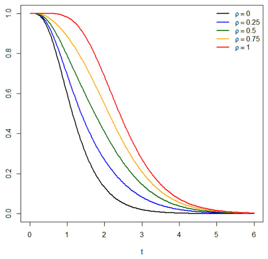
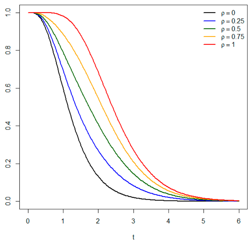
First, we examine the reliability performance of the proposed system for known parameter values. Figure 1 displays the reliability function for different values of , while the remaining design parameters are kept fixed (. The black, blue, dark green, orange, and red curves correspond to respectively.
Figure 1.
Reliability function of the system for .
As expected, larger values of lead to improved survival probabilities, since they correspond to a higher probability of successful activation of the spare system. The reliability curves are ordered with respect to . The black curve, corresponding to , represents the ordinary system without effective standby redundancy. The red curve, corresponding to , represents the perfect cold standby case. The blue, dark green, and orange curves describe the intermediate imperfect coverage cases. As increases, the survival curve shifts to the right, indicating improved system reliability and longer lifetime. The figure clearly illustrates the beneficial effect of the coverage probability on system reliability.
On the other hand, Table 1 presents the values of the Mean Time to Failure for different choices of and different designs of the structure. The component lifetimes are assumed to follow the exponential distribution with . The reported MTTF values were computed by the aid of (25).
Table 1.
for different coverage probabilities and system designs under exponential component lifetimes (.
The results confirm the direct effect of the coverage probability on the expected lifetime of the proposed system. For each fixed design, increases linearly with respect to . This behavior has been expected from the relation (17).
Table 1 also illustrates the effect of the design parameters. For the first group of designs, where , the Mean Time to Failure increases as the failure criteria become less restrictive. For instance, the value of for increases from for to for . A similar pattern is observed for the second group of designs, where .
Overall, Table 1 provides some numerical evidence that both the system design and the coverage probability have a substantial impact on the expected lifetime of the imperfect cold standby system. Larger values of improve system performance for all designs, while less restrictive failure thresholds lead to larger values of .
Table 2 presents the values of for selected time points, coverage probabilities, and three representative system designs. The component lifetimes are assumed to follow the exponential distribution with .
Table 2.
for different coverage probabilities and system designs.
For each fixed design and each fixed time , the Mean Residual Lifetime increases as the coverage probability increases. This confirms that imperfect standby activation has a positive effect not only on the initial lifetime of the system but also on its expected remaining lifetime after survival up to time . The smallest values correspond to , where the standby system provides no effective redundancy, while the largest values correspond to , which represents the perfect cold standby case.
It is also observed that, for each fixed value of , decreases as increases. That practically means that systems that have already operated for a longer time have a smaller expected remaining lifetime. For instance, for the design and , the Mean Residual Lifetime decreases from at to at .
Table 2 also illustrates the influence of the system’s design. More reliable designs lead to larger values of for all values of and examined. For example, when and , the corresponding values are and for , and respectively.
Finally, at , the Mean Residual Lifetime coincides with the Mean Time to Failure. This is consistent with the values reported in Table 1. However, for , the effect of on is no longer linear, since it also depends on the conditional lifetime distribution of the imperfect standby system given survival up to time .
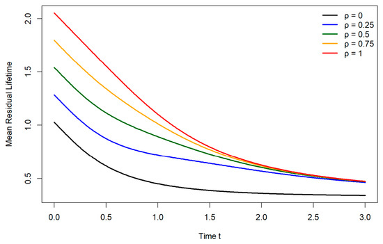
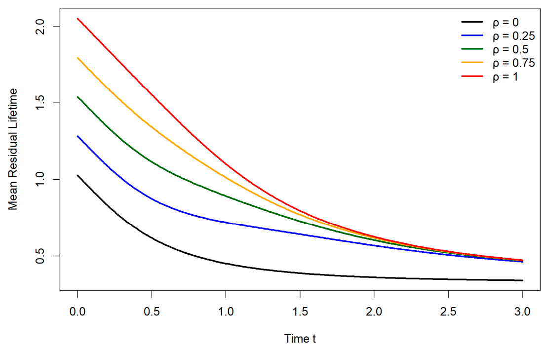
In addition to the numerical MRL values reported in Table 2, we also provide a graphical illustration of the Mean Residual Lifetime function. Figure 2 presents the MRL curves for the representative design (10,3,2,4), under exponential component lifetimes with = 1. The curves are displayed for 0, 0.25, 0.50, 0.75, and 1.
Figure 2.
Mean Residual Lifetime curves of the proposed imperfect standby system for (10,3,2,4), with = 1 and different values of .
The curves in Figure 2 provide some evidence that, for each fixed time point, the Mean Residual Lifetime increases as the coverage probability increases. This confirms the beneficial effect of the standby mechanism, since larger values of correspond to a higher probability of successful activation of the spare system. The curve corresponding to = 0 represents the ordinary system without standby contribution, whereas the curve corresponding to = 1 represents the perfect standby case. The intermediate curves lie between these two limiting cases and are ordered according to the value of .
A decreasing pattern is also observed as time increases for the considered exponential setting and system design. This indicates that, although the standby mechanism improves the remaining lifetime at all time points, the expected additional lifetime decreases as the system ages.
To illustrate the likelihood-based estimation procedure under right censoring, we consider the design and assume once again exponential component lifetimes with nominal parameter . Samples of sizes are generated for different values of the coverage probability and for two censoring levels. Kindly note that the target censoring level denotes the nominal censoring proportion used to generate the censoring times, whereas the observed censoring level is the actual proportion of censored observations obtained in each simulated sample. Since the samples are randomly generated, the observed censoring level may differ from the target one.
For each generated sample, the parameters are estimated by maximizing the censored-data log-likelihood described in Section 4.
Table 3 reports the maximum likelihood estimates of the model parameters together with their standard errors and 95% confidence intervals. The standard errors are obtained from the inverse of the observed information matrix evaluated at the maximum likelihood estimates. Confidence intervals are computed on the transformed parameter scale and then mapped back to the original parameter space, in order to respect the constraints > 0 and 0 < < 1.
Table 3.
Maximum likelihood estimates, standard errors, and 95% confidence intervals for the design under right censoring (nominal ).
The estimation procedure is summarized as follows. First of all, for the fixed system design , the signature vector of the ordinary system is computed. We then utilize the system-level imperfect standby representation to evaluate the reliability function and density function of the proposed system. Thirdly, independent system lifetimes are simulated from the imperfect standby model. Fourthly, independent censoring times are generated from an exponential distribution, with the censoring rate calibrated to achieve the desired nominal censoring proportion. The observed right-censored data are then formed as given in (19). Afterwards, the censored-data likelihood is maximized numerically to obtain the corresponding estimates, which are substituted into the theoretical expressions to obtain the corresponding plug-in estimates.
Table 3 offers some evidence that the proposed likelihood-based procedure can be implemented successfully for all numerical settings considered. The estimates of parameter are generally close to the true value (, especially for the larger sample sizes, while the confidence intervals provide additional information about the uncertainty of the estimates. The estimation of the coverage probability is more sensitive to sampling variation and censoring, which is expected since is associated with the successful activation of the spare system and is therefore indirectly observed through the system lifetime. This sensitivity is more pronounced for smaller samples and heavier censoring. Overall, Table 3 illustrates the practical feasibility of estimating both the component lifetime parameter and the coverage probability from right-censored system lifetime data.
By the aid of the estimates included in Table 3, we next compute plug-in estimates of the main reliability characteristics. More specifically, for each numerical setting, the estimates and are inserted into the reliability expressions derived in Section 3. The reliability function and the Mean Residual Lifetime are evaluated at . The Mean Time to Failure is computed from the corresponding plug-in expression (25) by substituting the respective maximum likelihood estimates for .
Table 4 presents the corresponding plug-in estimates of the reliability, the Mean Time to Failure, and the Mean Residual Lifetime. The results reflect the effect of the coverage probability on the reliability characteristics of the imperfect standby system. In general, larger values of the true coverage probability lead to larger estimated values of , , and . This is consistent with the theoretical results of Section 3 and with the numerical patterns observed in Table 1 and Table 2. Some non-monotonic fluctuations appear across sample sizes and censoring levels, due to the fact that the plug-in estimates depend on the likelihood estimates obtained from censored samples. Nevertheless, Table 4 demonstrates how the proposed inferential framework can be used to estimate practically relevant reliability characteristics when the model parameters are unknown.
Table 4.
Plug-in estimates of , for the design (true value of parameter ).
To further assess the finite-sample performance of the proposed maximum likelihood estimators, an additional Monte Carlo simulation study was conducted. We considered the representative system design (10,3,2,4), exponential component lifetimes with = 1, and coverage probability = 0.50. For each combination of sample size Ν = 50, 100, 200 and target censoring level 0.20, 0.40, Μ = 200, independent right-censored samples were generated.
For each simulated sample, the maximum likelihood estimates were computed, together with the corresponding 95% confidence intervals. The performance of the estimators was evaluated in terms of empirical bias, root mean squared error (RMSE), and empirical coverage probability (CP). The empirical coverage probability is defined as the proportion of valid replications in which the corresponding 95% confidence interval contains the true parameter value.
Table 5 reveals that the empirical biases of both estimators are small across all scenarios. The MSE and RMSE of generally decrease as the sample size increases, while the RMSE of also tends to decrease with larger samples, although it remains more sensitive to the censoring level.
Table 5.
Monte Carlo bias, RMSE, and empirical coverage probability of the maximum likelihood estimators for (10,3,2,4), with = 1 and = 0.50.
This behavior is expected, since directly controls the component lifetime distribution, whereas is not directly observed and it is inferred through the additional lifetime contribution associated with successful activation of the standby system. The empirical coverage probabilities are generally satisfactory, especially for . Overall, the Monte Carlo results support the stability and practical applicability of the proposed likelihood-based inference procedure under right censoring.
To further illustrate that the proposed framework is not restricted to exponential component lifetimes, we also consider an additional numerical setting under the Weibull distribution. More specifically, the component lifetimes are assumed to follow a Weibull distribution with shape parameter and scale parameter . The reliability function, the Mean Time to Failure, and the Mean Residual Lifetime are evaluated at for three representative system designs and selected values of the coverage probability .
Kindly note that the estimates of provide some evidence that greater variability exists compared to the corresponding one of λ, especially under small samples or heavier censoring. This is expected because is not directly observed; it is inferred indirectly through the additional lifetime contribution associated with successful standby activation. Heavy censoring reduces the information available in the upper tail of the lifetime distribution, where the effect of standby activation is more pronounced.
For all three designs depicted at Table 6, the reliability measures increase as the coverage probability increases. For instance, for the design (10,3,2,4), the estimated reliability at increases from 0.4560 for to 0.9992 for . Similarly, the corresponding Mean Time to Failure increases from 0.9843 to 1.9687.
Table 6.
Weibull numerical study for selected system designs and coverage probabilities.
A similar monotonic behavior is observed for the remaining designs. In particular, for (10,4,2,6), the Mean Time to Failure increases from 1.2402 when to 2.4803 when , while for (10,3,3,7), it increases from 1.3836 to 2.7672. These values are consistent with the theoretical relation according to which the Mean Time to Failure of the imperfect standby structure increases in terms of the coverage probability.
Table 6 also sheds light on the effect of the system design under Weibull component lifetimes. For fixed , the design (10,3,3,7) provides larger reliability measures than the (10,3,2,4) one, reflecting the less restrictive failure criteria of the former structure.
Overall, this additional numerical study demonstrates that the proposed formulae and computational procedure can be implemented for more flexible lifetime distributions, provided that the required integrations are evaluated numerically. Generally speaking, the computational implementation consists of three main steps: computation of the signature vector, numerical evaluation of the reliability and density functions, and numerical maximization of the censored-data likelihood. For moderate values of , the signature vector can be computed by the aid of subset enumeration. However, the enumeration cost increases with , since all failed component subsets may need to be checked. For larger systems, more efficient recursive algorithms or Monte Carlo approximations may be implemented. On the other hand, the numerical integrations appearing in the reliability expressions can be handled by standard quadrature methods, while the likelihood maximization is a low-dimensional constrained optimization problem in the examples considered here. However, more complex lifetime models may require multi-start optimization or Bayesian simulation-based methods.
6. Illustrative Applications
In this section, we present two illustrative applications of the proposed model to a linearly ordered monitoring system and a real dataset respectively. The simulated example is used to illustrate the proposed model in a setting that fully matches the assumed system structure and standby mechanism. In addition, a real right-censored automotive lifetime dataset is considered in order to demonstrate the implementation of the likelihood-based procedure with actual censored lifetime observations.
The first example is based on simulated right-censored lifetime data, generated under a realistic engineering scenario. Our aim is to shed light on how the proposed reliability structure can be applied when system-level lifetime observations are available and the underlying scheme is naturally described by combined consecutive-type failure criteria.
Consider a monitoring system consisting of sensors installed along an industrial conveyor system. The sensors are placed in a fixed linear order and are responsible for detecting abnormal operating conditions, local faults, or material-flow interruptions. In such systems, the relative positions of failed sensors are important. A small number of isolated sensor failures may not immediately stop the monitoring function, whereas a cluster of neighboring failed sensors may leave an entire segment of the line unobserved.
For this reason, the conveyor system is modeled as a structure. Under this design, the system fails if either four consecutive sensors fail or three non-overlapping pairs of consecutive failed sensors occur. The first criterion represents a severe local loss of monitoring ability, caused by a long consecutive block of failed sensors. The second criterion represents a more distributed deterioration of the monitoring system, where several smaller failure clusters appear in different parts of the line.
To improve reliability, the monitoring system is supported by a spare monitoring unit at the system level. The spare unit remains inactive during the operation of the primary system and is activated only after the primary system fails. However, in practice, the activation of the spare system may not always be successful. Possible reasons include communication delays, failure of the activation controller, or loss of power in the backup unit. Therefore, the assumption of perfect cold standby activation may be unrealistic in the above-mentioned setting. The system-level imperfect cold standby model considered in this paper provides a more flexible description of this situation.
The lifetime of the monitored system is assumed to follow the proposed imperfect standby model. Component lifetimes are generated from an exponential distribution with parameter , while the activation of the spare system is successful with probability . The illustrative dataset was generated from the proposed model with a fixed random seed and consist of system lifetimes subject to independent right censoring. Censoring may represent systems that are still operating at the end of the observation period, units removed from service for scheduled maintenance, or monitoring installations for which the failure time is not fully observed.
For the simulated dataset considered here, the observed censoring proportion is . That practically means that of the system lifetimes are right-censored. The unknown parameters are estimated by maximizing the censored-data log-likelihood introduced in Section 4. The resulting maximum likelihood estimates are
The estimate indicates the estimated failure rate of the individual monitoring components under the assumed exponential lifetime model. On the other hand, the estimated value suggests that, after failure of the primary monitoring system, the spare system is successfully activated with probability approximately . This value indicates a substantial but imperfect standby effect. Therefore, although the standby system improves the reliability of the monitoring installation, assuming perfect activation would overestimate the system performance.
Implementing the plug-in procedure described in Section 4, the estimated parameters are inserted into the reliability expressions derived in Section 3. At time , the estimated reliability of the resulting imperfect standby system is equal to
In simple words, the estimated probability that the monitoring system remains operational beyond time is approximately . Moreover, the estimated Mean Time to Failure is equal to
while the estimated Mean Residual Lifetime at time is given below
The latter value indicates that, conditional on the system having survived up to time , the expected additional operating time is approximately time units.
Overall, this illustrative application shows how the proposed framework can be used in a realistic reliability setting involving linearly ordered components, clustered failure patterns, right-censored lifetime observations, and imperfect standby activation. Although the data used here are simulated, the example demonstrates the practical implementation of the proposed likelihood-based inference procedure and the interpretation of the resulting reliability estimates.
In addition, it is of practical interest to examine the implementation of the proposed reliability measures in a real-data environment. For this purpose, we consider a real right-censored automotive lifetime dataset, originally reported by [22]. The data consist of failure and right-censored mileage observations from a fleet of vehicles on test. More specifically, the data include 10 observed failures and 21 right-censored observations. Therefore, the observed censoring proportion is 0.6774, which makes the data-set suitable for illustrating the proposed likelihood-based procedure under right censoring.
It should be noted that the dataset provides system-level lifetime observations and censoring indicators, but it does not contain information about the internal consecutive failure pattern of the components or the actual activation status of a standby system. Therefore, the present analysis is interpreted as a model-based real-data illustration of the proposed inferential framework. In particular, a Weibull lifetime model is first fitted to the observed right-censored mileage data. The fitted Weibull distribution is then used as the baseline system-level lifetime distribution, and the corresponding imperfect standby reliability measures are evaluated under several representative coverage scenarios.
Since the actual activation status of a standby unit is not recorded in the data, the coverage probability is treated as a prespecified design parameter in this real-data illustration. Therefore, the values are considered. This scenario-based analysis allows us to examine the effect of the coverage probability on the reliability characteristics of the fitted system-level lifetime model, without overinterpreting ρ from data that do not directly contain standby activation information.
The mileage observations are divided by 100.000 before fitting the Weibull model. Consequently, corresponds to 100.000 miles. The maximum likelihood estimates of the Weibull parameters are and , with standard errors 0.2961 and 0.4277, respectively (see Table 7).
Table 7.
Weibull parameter estimates for the real automotive censored lifetime data.
The corresponding 95% confidence intervals are (0.6982, 1.9086) for and (0.7225, 2.5094) for . Since the scale parameter is expressed in units of 100.000 miles, the fitted value corresponds to approximately 134.650 miles.
Table 8 reports the plug-in standby reliability estimates under the different fixed coverage scenarios. The results show a clear improvement as increases.
Table 8.
Plug-in standby reliability estimates for the real automotive censored lifetime data.
In particular, increases from 0.4920 for to 0.8595 for . Similarly, increases from 128.005 miles to 256.010,1 miles, while increases from 110.757,3 miles to 187.024,2 miles. The doubling of under is consistent with the system-level standby representation .
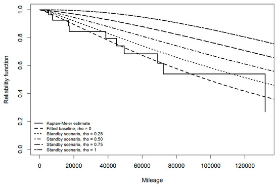
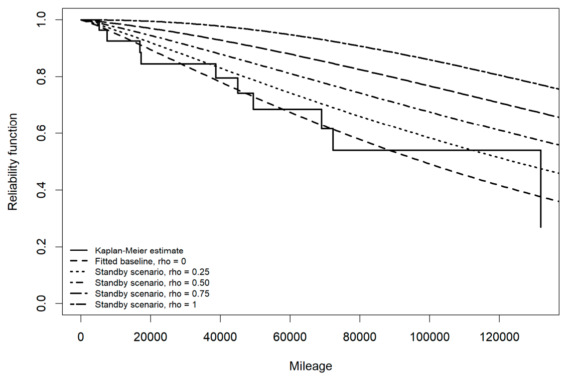
Figure 3 compares the Kaplan–Meier estimate obtained from the automotive censored data with the fitted Weibull baseline reliability curve and the plug-in imperfect standby reliability curves. The fitted standby curves lie above the baseline curve and are ordered according to the value of , confirming the expected reliability improvement induced by the standby mechanism.
Figure 3.
Kaplan–Meier estimate, fitted Weibull baseline reliability curve, and plug-in imperfect standby reliability curves under different fixed coverage scenarios for the automotive censored lifetime data.
The graphical results in Figure 3 are consistent with the numerical findings in Table 6 and Table 7. The fitted baseline Weibull curve captures the general decreasing pattern of the Kaplan–Meier estimate. The plug-in standby reliability curves are positioned above the baseline curve and increase as the coverage probability becomes larger. This behavior agrees with the theoretical role of the imperfect standby mechanism, since larger values of correspond to a higher probability of successful standby activation and therefore to improved system reliability.
7. Discussion
In this paper, we studied a combined -consecutive--out-of-: F and consecutive -out-of-: F system under imperfect cold standby redundancy at the system level. The proposed model introduces a coverage probability , which represents the probability of successful activation of the spare system. Therefore, the cases and correspond to the ordinary system without effective standby redundancy and to the perfect cold standby model, respectively. The present model is distinct from many existing imperfect standby formulations because it combines the system-level coverage probability with a two-criterion consecutive-type failure structure. Therefore, we attempt the extension of perfect standby models to an imperfect activation setting for combined consecutive-type systems.
Signature-based expressions were obtained for the reliability function, the Mean Time to Failure, and the Mean Residual Lifetime of the proposed structure. The numerical results showed that larger values of lead to improved system performance.
A likelihood-based procedure was developed for estimating the unknown component lifetime parameter and the coverage probability from right-censored system lifetime data. The plug-in estimates of , , and provide reliability measures for practical assessment and maintenance planning. The above-mentioned procedure is based on independent random right censoring. If the censoring mechanism depends on the system lifetime, the likelihood formulation based on independent censoring may no longer be valid, and the resulting estimators may be biased. Such dependent censoring may occur, for example, when units exposed to more severe operating conditions are also more likely to be withdrawn from observation. In such cases, additional modeling of the censoring mechanism, joint modeling approaches, or sensitivity analyses would be required.
The present study focused on imperfect cold standby redundancy at the system level. A natural direction for future research is the corresponding component-level scheme, where each primary component is equipped with its own spare unit and the activation of each spare component may be imperfect. Such an extension would require the derivation of the effective component lifetime distribution and the development of the corresponding reliability and inferential results.
For more general lifetime distributions, complex standby mechanisms, or component-level imperfect coverage schemes, closed-form expressions may not always be available or may become analytically cumbersome. In such cases, numerical approximation, simulation-based procedures, and Bayesian methods, such as Markov chain Monte Carlo techniques, may provide useful alternatives for reliability estimation and uncertainty quantification.
On the other hand, it is true that the present study assumes independent and identically distributed component lifetimes. This assumption allows the implementation of the system signature representation and leads to tractable reliability and likelihood expressions. However, in some engineering systems, component lifetimes may exhibit spatial or environmental dependence. In such cases, the standard signature representation may need to be replaced by more general tools such as survival signatures or copula-based dependence models. Extending the proposed inferential framework to dependent component lifetimes seems to be an important direction for future research.
Funding
This research received no external funding.
Data Availability Statement
No empirical or externally sourced datasets were used in this study. The numerical examples in the application section are based solely on simulated/synthetic data generated according to the simulation design described in the manuscript. The simulated data and/or code used to generate them are available from the corresponding author upon reasonable request.
Conflicts of Interest
The author declare no conflicts of interest.
References
- Kontoleon, J.M. Reliability determination of a r-successive-out-of-n: F system. IEEE Trans. Reliab. 1980, 29, 437. [Google Scholar] [CrossRef] [Scilit]
- Chiang, N.; Niu, S. Reliability of consecutive-k-out-of-n: F system. IEEE Trans. Reliab. 1981, 30, 87–89. [Google Scholar] [CrossRef] [Scilit]
- Derman, C.; Lieberman, G.J.; Ross, S.M. On the consecutive-k-out-of-n: F system. IEEE Trans. Reliab. 1982, 31, 57–63. [Google Scholar] [CrossRef] [Scilit]
- Tong, Y.L. A rearrangement inequality for the longest run, with an application to network reliability. J. Appl. Probab. 1985, 22, 386–393. [Google Scholar] [CrossRef] [Scilit]
- Kumar, A.; Singh, S.B. Signature reliability of A-within-B-from-D/G sliding window system. Int. J. Math. Eng. Manag. Sci. 2019, 4, 95–107. [Google Scholar] [CrossRef] [Scilit]
- Triantafyllou, I.S.; Koutras, M.V. Signature and IFR preservation of 2-within-consecutive k-out-of-n: F systems. IEEE Trans. Reliab. 2011, 60, 315–322. [Google Scholar] [CrossRef] [Scilit]
- Griffith, W.S. On Consecutive-k-out-of-n failure systems and their generalizations. In Reliability and Quality Control; Basu, A.P., Ed.; Elsevier: Amsterdam, The Netherlands, 1986; pp. 157–165. [Google Scholar]
- Papastavridis, S. m-consecutive-k-out-of-n: F systems. IEEE Trans. Reliab. 1990, 39, 386–388. [Google Scholar]
- Triantafyllou, I.S. An Archimedean Copulas-Based Approach for m-Consecutive-k-out-of-n: F Systems with Exchangeable Components. Stats 2023, 6, 1114–1125. [Google Scholar] [CrossRef] [Scilit]
- Chang, J.G.; Cui, L.; Hwang, F.K. Reliabilities for (n,f,k) systems. Stat. Probab. Lett. 1999, 43, 237–242. [Google Scholar] [CrossRef] [Scilit]
- Triantafyllou, I.S.; Chalikias, M. Consecutive k1- and k2-out-of-n reliability systems with a single change point. Stats 2023, 6, 438–449. [Google Scholar] [CrossRef] [Scilit]
- Eryilmaz, S.; Zuo, M.J. Constrained (k,d)-out-of-n systems. Int. J. Syst. Sci. 2010, 41, 679–685. [Google Scholar] [CrossRef] [Scilit]
- Eryilmaz, S. Reliability of Combined m-consecutive-k-out-of-n: F & consecutive-kc-out-of-n: F systems. IEEE Trans. Reliab. 2012, 61, 215–219. [Google Scholar] [CrossRef]
- Mohan, P.; Agarwal, M.; Sen, K. Combined m-consecutive-k-out-of-n: F & consecutive-kc-out-of-n: F systems. IEEE Trans. Reliab. 2009, 58, 328–337. [Google Scholar] [CrossRef]
- Eryilmaz, S.; Unlu, K.D. A new generalized δ-shock model and its application to 1-out-of-(m+1):G cold standby system. Reliab. Eng. Syst. Saf. 2023, 234, 109203. [Google Scholar] [CrossRef] [Scilit]
- Boland, P.J.; El-Neweihi, E. Component redundancy vs system redundancy in the hazard rate ordering. IEEE Trans. Reliab. 1995, 44, 614–619. [Google Scholar] [CrossRef] [Scilit]
- Eryilmaz, S. The effectiveness of adding cold standby redundancy to a coherent system at system and component levels. Reliab. Eng. Syst. Saf. 2017, 165, 331–335. [Google Scholar] [CrossRef] [Scilit]
- Triantafyllou, I.S. Combined m-consecutive-k-out-of-n: F & consecutive kc-out-of-n: F structures with cold standby redundancy. Mathematics 2023, 11, 2597. [Google Scholar] [CrossRef] [Scilit]
- Cramer, E. Ordered and censored lifetime data in reliability: An illustrative review. Wiley Interdiscip. Rev. Comput. Stat. 2023, 15, e1571. [Google Scholar]
- van der Vaart, A.W. Asymptotic Statistics; Cambridge University Press: Cambridge, UK, 1998. [Google Scholar]
- Meeker, W.Q.; Escobar, L.A. Statistical Methods for Reliability Data; Wiley: New York, NY, USA, 2014. [Google Scholar]
- Krivtsov, V.; Case, J. Peculiarities of Censored Data Analysis in Automotive Industry Applications. In International Body Engineering Conference & Exposition; SAE International: Detroit, MI, USA, 1999. [Google Scholar] [CrossRef] [Scilit]

Disclaimer/Publisher’s Note: The statements, opinions and data contained in all publications are solely those of the individual author(s) and contributor(s) and not of MDPI and/or the editor(s). MDPI and/or the editor(s) disclaim responsibility for any injury to people or property resulting from any ideas, methods, instructions or products referred to in the content. |
© 2026 by the author. Licensee MDPI, Basel, Switzerland. This article is an open access article distributed under the terms and conditions of the Creative Commons Attribution (CC BY) license.