Information-Preserving and Model-Aware Voronoi Dequantization of Weighted Discrete Laws

Abstract

Continuous dequantization embeds discrete data into a continuous space, but relaxation can alter the statistical information carried by the original categories. We study a complementary regime in which a specified weighted discrete law is the target and the dequantizer is required to be lossless under a prescribed quantizer. Any partition-respecting, parameter-independent kernel produces a continuous experiment Blackwell equivalent to the original discrete one, so likelihood ratios, maximum-likelihood estimators, score and Fisher information, Bayes posteriors, and optimal risks are unchanged before downstream approximation. We then characterize what happens after a finite-capacity continuous model is fitted. A Kullback–Leibler (KL) chain rule separates continuous approximation error into the categorical error of the requantized model plus a within-cell shape term; the information-preservation guarantee therefore does not extend automatically to an arbitrary fitted downstream model. We also provide a plug-in analysis for empirically estimated weights, showing that dequantization preserves rather than removes the discrete estimation error. Within each cell, maximizing entropy minus a displacement penalty yields a truncated Gibbs kernel. The apparent concentration and geometric-scale parameters reduce exactly to one effective concentration, $\alpha =\lambda /s_c^2$. We further derive exact transport costs, a sharp $W_1=\Theta \left(h^2\right)$ reconstruction rate for the special reconstruction-from-exact-bin-masses setting, leakage-specific and geometry-perturbation bounds, and a bounded-domain multidimensional formulation. A finite-candidate Monte Carlo selector satisfies a nonasymptotic $O\left(m^{-1/2}\right)$ oracle inequality. Experiments verify the identities and show that exact dequantization can materially reduce requantized error when a smooth continuous downstream model is imposed; this is a conditional representational advantage, not a claim that dequantization dominates an unrestricted categorical model.

1. Introduction

Let $P_X={\sum }_{i=1}^n{p}_i{\delta }_{x_i}$ be a known discrete probability law. A common machine-learning workflow replaces the atoms with a continuous random variable before fitting a continuous-density model. For integer-valued data, uniform dequantization adds a fixed-width uniform perturbation to each category; this device is standard in neural autoregressive models and normalizing flows [1,2,3,4]. More general dequantization objectives and learned conditional dequantizers have been developed specifically to bridge discrete and continuous likelihood models [5]. Fixed width is natural when the discrete values are equally spaced, but not when the support carries a meaningful, irregular numeric geometry.

More broadly, the representation problem is not unique to dequantization: recent statistical work has emphasized that continuous model construction should respect support, identifiability, entropy, and the information contained in the observed representation. Examples include bounded and lifetime distribution models in which reparameterization or shape constraints determine the effective model class [6,7,8], and uncertainty-aware methods that retain interval or soft-data information rather than collapsing it to a single point [9,10]. These studies address different inferential problems, but they reinforce the general principle motivating the present work: a convenient continuous representation should not silently discard structure that is relevant to the downstream statistical task.

The geometric idea of spreading point mass over Voronoi cells is not new. Classical Voronoi density estimators assign density inversely proportional to cell volume, and recent work has developed compactified and continuous variants for density estimation from samples [11,12]. Chen, Amos, and Nickel [13] introduced learned Voronoi dequantization inside semi-discrete normalizing flows. These papers make it inappropriate to claim novelty for a piecewise-constant Voronoi formula itself.

This paper asks a narrower but, we believe, useful question: what exact probabilistic structure is obtained when a known weighted discrete law is dequantized on a prescribed geometric partition? That change in viewpoint produces several properties that are directly relevant to statistical computation and that are not the usual focus of sample-based Voronoi density estimation.

Our contributions are as follows:

1.

We formulate partition-respecting dequantization as a Markov kernel and prove exact requantization. For parameterized weight vectors, the discrete and continuous experiments are Blackwell equivalent [14,15]; hence, exact dequantization is lossless for statistical decision making.

2.

We prove exact likelihood and f-divergence preservation for a common parameter-independent kernel. We then derive a downstream KL chain rule: after fitting an arbitrary continuous density, its KL error decomposes exactly into requantized categorical KL plus a weighted within-cell approximation term.

3.

We use that decomposition to separate representation fidelity from model capacity. A continuous model can waste approximation capacity on within-cell shape, even when all exact dequantizers contain the same discrete information. This yields a model-aware kernel-selection criterion based on requantized loss, together with a finite-sample oracle inequality when categorical risk is estimated by Monte Carlo requantization.

4.

We solve an entropy–transport variational problem over all exact cell-confined kernels. The unique solution is a truncated Gibbs family $k_{i,\lambda }\propto \exp \{-\lambda c_i\}$; $\lambda =0$ is the maximum-entropy uniform kernel, while increasing $\lambda$ decreases expected displacement monotonically without sacrificing exact requantization.

5.

We quantify two specific perturbation effects: category leakage bounds requantization error for approximate kernels, while a geometry-perturbation bound controls the effect of using perturbed support sites or quantization boundaries.

6.

For Voronoi cells, we obtain the exact $W_r$ transport cost to the atomic law, closed-form one-dimensional density/CDF/quantile formulas, and a sharp $W_1=\Theta \left(h^2\right)$ result for the distinct special case of reconstructing a smooth law from its exact bin masses. A bounded-domain formulation handles multidimensional cells correctly.

7.

Reproducible experiments verify the exact inference/divergence/KL identities, compare ten-seed Gaussian-mixture capacity curves, validate model-aware selection with bounded rational-quadratic spline normalizing flows, audit finite-sample selector regret and geometry perturbations, and include a real irregular-spacing example.

The proposed framework should therefore be viewed as an information-preserving and model-aware dequantization framework, not as a new nonparametric density estimator. The geometry fixes which continuous draws decode to each discrete state; the within-cell kernel can then be chosen to balance entropy, transport, and downstream approximation while preserving the target PMF exactly.

The model-aware component also makes validation design part of the method. Recent work on adaptive thresholds, deployment auditing under distribution shift, and risk-gated recalibration has similarly separated data-driven model or threshold selection from held-out or prospective evaluation [16,17,18]. The present problem is different–the candidate kernels are exact right inverses before downstream approximation–but the same validation principle applies once kernel selection and continuous-model fitting are learned from finite data.

2. Relation to Existing Voronoi and Dequantization Methods

2.1. Uniform and Learned Dequantization

Uniform dequantization adds independent uniform noise to integer-like observations. The continuous likelihood can then be related to the discrete likelihood, while variational and importance-weighted dequantization learn or optimize more flexible conditional noise distributions [2,4,5]. Nielsen and Winther [19] identified the usual variational dequantization gap as a conditional KL term, and that truncated-flow dequantizers can enforce non-overlapping bounded supports while remaining trainable [20]. These studies optimize a generative likelihood for unknown data distributions. The present regime instead takes the weighted discrete law as the target itself: support points may be irregularly spaced, exact requantization is required, and we ask which exact within-cell kernel is most convenient for a restricted downstream continuous model.

Chen et al. [13] used Voronoi cells inside a learned semi-discrete flow, including multidimensional learned quantization boundaries. Their contribution is substantially more expressive computationally. Our goal is complementary: a closed-form deterministic operator with exact requantization, exact divergence preservation, and no learned tessellation. To test whether the model-aware effect persists beyond Gaussian mixtures, Section 6.5 uses monotone rational-quadratic spline flows, a flexible analytically invertible normalizing-flow transformation introduced by Durkan et al. [21].

2.2. Voronoi Density Estimation

The VDE literature starts from samples of an unknown continuous law. A Voronoi tessellation is constructed from the sample, and density is related to the inverse cell volume. Polianskii et al. [11] emphasized both the computational difficulty of high-dimensional Voronoi cells and the need for compactification; Marchetti et al. [12] developed a continuous radial VDE. In contrast, here, $p_i$ is known, and the cell integral is required to be exactly $p_i$. On a bounded domain, the resulting density formula coincides with a weighted piecewise-constant VDE. We explicitly acknowledge this overlap; the contribution lies in the dequantization/right-inverse and information-preservation characterization.

3. Partition-Respecting Dequantization

3.1. General Construction

Let $\Omega \subset {\mathbb{R}}^d$ be bounded and measurable. Let $C_1,\dots ,C_n$ form a measurable partition of $\Omega$ up to null sets, with $0<\mathrm{Vol}\left(C_i\right)<\infty$. Associate one discrete state $x_i$ with each cell and define the quantizer

$$Q\left(y\right)=x_i,y\in C_i.$$

For a weight vector $p=(p_1,\dots ,p_n)$ in the probability simplex, define

$$\left(T_{C}p\right)\left(y\right)={\displaystyle \sum _{i=1}^n}{\displaystyle \frac{p_i}{\mathrm{Vol}\left(C_i\right)}}{\mathbf{1}}_{C_i}\left(y\right).$$

(1)

Equivalently, sample $X=x_i$ with probability $p_i$, then sample $Y\mid X=x_i\sim \mathrm{Unif}\left(C_i\right)$.

Theorem 1 

(Exact stochastic right inverse). Under the coupled construction above, $Q\left(Y\right)=X$ almost surely. Consequently,

$$Q_{\#}\left(T_{C}p\right)=P_X,P\{Q\left(Y\right)=x_i\}=p_i\mathit{for}\mathit{every}i.$$

Proof. 

Conditional on $X=x_i$, the draw Y belongs to $C_i$ with probability one, and $Q\left(y\right)=x_i$ on that cell. Integrating over X provides the stated marginal identity.    □

This property is stronger than saying that the continuous density integrates to one: it says the continuous representation retains the discrete law exactly under its associated quantizer.

3.2. Blackwell Equivalence and Likelihood Preservation

The right-inverse property has a stronger statistical interpretation. Let $\{p_{\theta }:\theta \in \Theta \}$ be any parameterized family of weights on the fixed support, and let $K(dy\mid x_i)=k_i\left(y\right)dy$ be a kernel that does not depend on $\theta$, with $k_i$ supported on $C_i$. Let ${\mathcal{E}}_X=\left\{P_{\theta }^X\right\}$ denote the discrete experiment and ${\mathcal{E}}_Y=\left\{P_{\theta }^Y\right\}$ its dequantized version.

Theorem 2 

(Lossless statistical experiment). The experiments ${\mathcal{E}}_X$ and ${\mathcal{E}}_Y$ are Blackwell equivalent. The kernel K maps $P_{\theta }^X$ to $P_{\theta }^Y$, while the deterministic kernel induced by Q maps $P_{\theta }^Y$ back to $P_{\theta }^X$ for every θ. Therefore, they have the same attainable risk set for every statistical decision problem.

If additionally $p_{\theta ,i}>0$ on the parameter region of interest, then for $y\in C_i$,

$$\log f_{\theta }\left(y\right)=\log p_{\theta ,i}+\log k_i\left(y\right).$$

For an i.i.d. sample, the continuous and discrete log-likelihoods differ only by a θ-free additive term. Consequently, their likelihood ratios, MLEs, score functions, observed information, and Fisher information coincide; with the same prior, their Bayes posteriors also coincide after applying Q.

Proof. 

The first statement follows because $P_{\theta }^Y=P_{\theta }^{X}K$, and Theorem 1 provides $P_{\theta }^X=P_{\theta }^{Y}Q$ for every $\theta$, which is precisely mutual garbling in the sense of Blackwell. On $C_i$, disjoint support yields $f_{\theta }\left(y\right)=p_{\theta ,i}{k}_i\left(y\right)$, proving the likelihood identity. Every stated likelihood-based consequence follows because the added kernel term is independent of $\theta$.    □

The general comparison-of-experiments theory is classical [14,15]; the point here is that exact partition-respecting dequantization furnishes the two Markov kernels explicitly. Thus, continuous relaxation can be statistically lossless for inference on the weight vector even though a finite-capacity downstream density model may later introduce approximation error.

3.3. Exact Preservation of Information Divergences

Let p and q be two weight vectors on the same support and use the same partition. For a convex function $\varphi$ with $\varphi \left(1\right)=0$, the Csiszár f-divergence is

$$D_{\varphi }(P\parallel Q)=\int q\left(y\right)\varphi \left({\displaystyle \frac{p\left(y\right)}{q\left(y\right)}}\right)dy,$$

with the usual conventions at zero mass.

Theorem 3 

(f-divergence isometry). For every f-divergence for which the two sides are defined,

$$D_{\varphi }(T_{C}p\parallel T_{C}q)=D_{\varphi }(p\parallel q)={\displaystyle \sum _{i=1}^n}{q}_i\varphi \left({\displaystyle \frac{p_i}{q_i}}\right).$$

In particular,

$$\mathrm{TV}(T_{C}p,T_{C}q)=\mathrm{TV}(p,q),\mathrm{KL}(T_{C}p\parallel T_{C}q)=\mathrm{KL}(p\parallel q),$$

and the squared Hellinger distance is also preserved exactly.

Proof. 

On $C_i$, the ratio $\left(T_{C}p\right)/\left(T_{C}q\right)$ equals $p_i/q_i$. Therefore,

$${\int }_{C_i}{\displaystyle \frac{q_i}{\mathrm{Vol}\left(C_i\right)}}\varphi \left({\displaystyle \frac{p_i}{q_i}}\right)dy=q_i\varphi \left({\displaystyle \frac{p_i}{q_i}}\right).$$

Summing over cells proves the result.    □

Remark 1. 

Theorem 3 does not require uniformity inside a cell. It remains true whenever both p and q are dequantized with the same conditional density $k_i\left(y\right)$ supported on $C_i$, because the factor $k_i$ cancels in the likelihood ratio. Uniformity is selected by entropy, not by divergence preservation.

• Estimated weights and plug-in dequantization.

The exact right-inverse and Blackwell statements above concern the discrete law supplied to the dequantizer. When the population weights p are unknown, and an empirical vector $\widehat{p}$ is inserted instead, the exact guarantees hold conditionally for $\widehat{p}$; they do not erase the sampling error between p and $\widehat{p}$. This distinction is especially simple for a common fixed cell-confined kernel K. Because the cells are disjoint,

$$\mathrm{TV}(T_{K}p,T_K\widehat{p})=\mathrm{TV}(p,\widehat{p}),$$

(2)

and, under the same absolute-continuity conditions as Theorem 3, $D_{\varphi }(T_{K}p\parallel T_K\widehat{p})=D_{\varphi }(p\parallel \widehat{p})$. Thus, plug-in dequantization neither amplifies nor contracts the discrepancy caused by estimating the weights; it transports that discrepancy exactly into the continuous representation.

If $\widehat{p}$ is the empirical PMF from N independent draws from an n-category law p, then

$$E\mathrm{TV}(p,\widehat{p})\le {\displaystyle \frac{1}{2}}\sqrt{{\displaystyle \frac{n-1}{N}}},\mathrm{TV}(p,\widehat{p})\le {\displaystyle \frac{1}{2}}\sqrt{{\displaystyle \frac{n-1}{N}}}+\sqrt{{\displaystyle \frac{\log (1/\delta )}{2N}}}$$

(3)

with probability at least $1-\delta$. The expectation bound follows from Cauchy–Schwarz and $E\parallel \widehat{p}{-p\parallel }_2^2={(1-\parallel p\parallel }_2^2)/N$; the deviation term follows from bounded differences because replacing one observation changes TV by at most $1/N$. For KL, an unsmoothed empirical PMF can assign zero mass to a population-positive category and, therefore, produce infinite KL; smoothing or a model that enforces positive category mass is required when a finite KL comparison is desired.

When the same finite dataset is used to estimate p, choose the dequantizer and fit the downstream model. The selection procedure itself can overfit even though the conditional dequantization map is exact. A practical implementation should therefore separate fitting and selection—for example, by a training/validation split, nested validation, or cross-fitting. The real-data experiments below use outer held-out folds and an inner validation subset for choosing the Gibbs concentration.

3.4. Downstream Approximation and the Categorical KL Decomposition

Blackwell equivalence describes the relaxation before an approximating continuous model is imposed. The next identity isolates the error created by such an approximation.  Let

$$f_p\left(y\right)=\sum _i{p}_i{k}_i\left(y\right),\mathrm{supp}\left(k_i\right)\subseteq C_i,$$

and let q be any density on the same domain. Define its induced category probabilities

$${\widehat{p}}_i={\int }_{C_i}q\left(y\right)dy,$$

and, whenever ${\widehat{p}}_i>0$, its within-cell conditional density $r_i\left(y\right)=q\left(y\right)/{\widehat{p}}_i$ for $y\in C_i$.

Theorem 4 

(Downstream KL decomposition). Assume $p_i>0$ implies ${\widehat{p}}_i>0$ and $k_i\ll r_i$. Then,

$$\mathrm{KL}(f_p\parallel q)=\mathrm{KL}(p\parallel \widehat{p})+{\displaystyle \sum _{i=1}^n}{p}_i\mathrm{KL}(k_i\parallel r_i).$$

(4)

Consequently, $\mathrm{KL}(p\parallel \widehat{p})\le \mathrm{KL}(f_p\parallel q)$. More generally, for every f-divergence,

$$D_{\varphi }\{p\parallel Q_{\#}q\}\le D_{\varphi }(f_p\parallel q),$$

by data processing through Q.

Proof. 

On $C_i$, $f_p=p_i{k}_i$ and $q={\widehat{p}}_i{r}_i$. Therefore,

$${\int }_{C_i}{p}_i{k}_i\log {\displaystyle \frac{p_i{k}_i}{{\widehat{p}}_i{r}_i}}=p_i\log {\displaystyle \frac{p_i}{{\widehat{p}}_i}}+p_i\mathrm{KL}(k_i\parallel r_i).$$

Summation proves (4). The f-divergence inequality is the data-processing inequality for the deterministic Markov kernel Q.    □

The coverage condition in Theorem 4 is substantive. For every target-positive cell, the fitted density must place positive mass on the cell, and its within-cell conditional density must dominate $k_i$ on the support of $k_i$. If this fails, the relevant KL terms are $+\infty$ and the identity remains only an extended-valued equality, not a finite categorical-versus-shape decomposition. The Gaussian-mixture fits used below have positive density on all of $\mathbb{R}$, and the bounded spline flows used in the audits have positive density throughout the modeled domain, so cell coverage is 100% in the experiments where the finite decomposition is interpreted. A truncated or compact-support model that leaves part of a target cell uncovered must instead be reported as a coverage failure.

The first term in (4) is the error in the discrete law recovered after fitting q; the second is a within-cell shape penalty that can consume finite model capacity without changing the target categories. Thus, two exact dequantizers can be statistically equivalent before approximation but differ substantially in how easy they are for a restricted class $\mathcal{F}$ to fit. For a family of exact kernels $k_{\lambda }$, a natural model-aware criterion is

$${\lambda }_{\mathcal{F}}^{*}\in \arg \underset{\lambda }{\min }D\left(p,Q_{\#}{\widehat{q}}_{\lambda ,\mathcal{F}}\right),{\widehat{q}}_{\lambda ,\mathcal{F}}\approx \arg \underset{q\in \mathcal{F}}{\min }\mathrm{KL}(f_{p,\lambda }\parallel q),$$

where D may be TV or categorical KL. Because p is the specified target law, this criterion can be evaluated directly. For parametric inference across unknown $p_{\theta }$, however, the dequantization kernel must remain $\theta$-independent for Theorem 2 to apply.

Theorem 5 

(Finite-sample oracle inequality for Monte Carlo kernel selection). Let Λ be a finite set of M exact dequantizers and condition on fitted downstream densities $\{q_{\lambda }:\lambda \in \Lambda \}$. Write $r_{\lambda }=Q_{\#}{q}_{\lambda }$ and $R\left(\lambda \right)=\mathrm{TV}(p,r_{\lambda })$. For each λ, generate m draws from $q_{\lambda }$, requantize them, let ${\widehat{r}}_{\lambda ,m}$ be the resulting empirical categorical law, and define

$$\widehat{\lambda }\in \arg \underset{\lambda \in \Lambda }{\min }\mathrm{TV}(p,{\widehat{r}}_{\lambda ,m}).$$

Then, for every $0<\delta <1$, with probability at least $1-\delta$ over the Monte Carlo draws,

$$R\left(\widehat{\lambda }\right)\le \underset{\lambda \in \Lambda }{\min }R\left(\lambda \right)+\sqrt{{\displaystyle \frac{n-1}{m}}}+2\sqrt{{\displaystyle \frac{\log (M/\delta )}{2m}}}.$$

(5)

If the categorical masses $r_{\lambda }\left(C_i\right)$ are available analytically, the Monte Carlo term is unnecessary and the best candidate in Λ can be selected exactly conditional on the fitted models.

Proof. 

For fixed $\lambda$, the reverse triangle inequality provides $|\mathrm{TV}(p,{\widehat{r}}_{\lambda ,m})-\mathrm{TV}(p,r_{\lambda })|\le \mathrm{TV}({\widehat{r}}_{\lambda ,m},r_{\lambda })$. Moreover,

$$E\mathrm{TV}({\widehat{r}}_{\lambda ,m},r_{\lambda })\le {\displaystyle \frac{1}{2}}\sqrt{{\displaystyle \frac{n-1}{m}}},$$

because $E\parallel \widehat{r}{-r\parallel }_1\le \sqrt{nE\parallel \widehat{r}{-r\parallel }_2^2}$ and $E\parallel \widehat{r}{-r\parallel }_2^2={(1-\parallel r\parallel }_2^2)/m\le (n-1)/\left(nm\right)$. Changing one generated category changes TV by at most $1/m$, so McDiarmid’s inequality and a union bound over M candidates imply, with probability at least $1-\delta$,

$$\underset{\lambda \in \Lambda }{\sup }|\mathrm{TV}(p,{\widehat{r}}_{\lambda ,m})-R\left(\lambda \right)|\le {\displaystyle \frac{1}{2}}\sqrt{{\displaystyle \frac{n-1}{m}}}+\sqrt{{\displaystyle \frac{\log (M/\delta )}{2m}}}.$$

The empirical minimizer is therefore within twice this uniform error of the oracle risk, proving (5).    □

3.5. Approximate Right Inverses and a Leakage Bound

Exact cell confinement is a sharp idealization for learned or globally smoothed dequantizers. Let an arbitrary kernel $K_i$ generate Y from $X=x_i$, retain the same quantizer Q, and define the weighted category-mismatch probability

$${ϵ}_p={\displaystyle \sum _{i=1}^n}{p}_i{K}_i\{y:Q\left(y\right)\ne x_i\}.$$

Proposition 1 

(Requantization bound under category leakage). If ${\tilde{P}}_X=Q_{\#}{P}_Y$ is the law obtained after dequantization and requantization, then

$$\mathrm{TV}(P_X,{\tilde{P}}_X)\le {ϵ}_p.$$

In particular, every exact partition-respecting dequantizer has ${ϵ}_p=0$ and zero requantization error.

Proof. 

Use the natural coupling that first draws X and then draws $Y\mid X$. Under this coupling, $P\{Q\left(Y\right)\ne X\}={ϵ}_p$. The coupling characterization of total variation yields the bound.    □

This inequality supplies a model-independent diagnostic for approximate dequantizers. It also separates two effects that are sometimes conflated: probability mass may leave a chosen bounded plotting domain without changing category after nearest-neighbor requantization, whereas crossing an internal quantization boundary contributes directly to ${ϵ}_p$.

A second perturbation question arises when the dequantizer is exact for one geometry but decoding uses perturbed sites or boundaries. Let $\widehat{Q}$ have cells ${\widehat{C}}_i$ carrying the same labels as $C_i$.

Proposition 2 

(Bound under quantizer-geometry perturbation). If $Y\mid X=x_i\sim K_i$ with $K_i\left(C_i\right)=1$ and $\widehat{p}$ is the law of $\widehat{Q}\left(Y\right)$, then

$$\mathrm{TV}(p,\widehat{p})\le \sum _i{p}_i{K}_i(C_i\setminus {\widehat{C}}_i)\le \sum _i{p}_i{K}_i(C_i▵{\widehat{C}}_i).$$

For the one-dimensional uniform Voronoi kernel, if the ordered sites are perturbed to ${\widehat{x}}_i$ with ${\max }_i|{\widehat{x}}_i-x_i|\le \delta$ and their order is preserved, then

$$\mathrm{TV}(p,\widehat{p})\le \sum _i{p}_i\min \left(1,{\displaystyle \frac{2\delta }{{\Delta }_i}}\right).$$

(6)

Proof. 

Couple $X,Y$ as before and decode Y using $\widehat{Q}$. Conditional error in category i is $K_i(C_i\setminus {\widehat{C}}_i)$, so the first inequality follows from the coupling bound for TV. The second is immediate. In one dimension, every internal midpoint moves by at most $\delta$; hence, at most $2\delta$ of an original interval of width ${\Delta }_i$ can be relabeled. Uniformity within the cell provides (6).    □

3.6. Maximum-Entropy and Entropy–Transport Exact Kernels

Consider all partition-respecting kernels $k_i$ supported on $C_i$ and integrating to one. Their mixture density is $f\left(y\right)={\sum }_i{p}_i{k}_i\left(y\right)$.

Theorem 6 

(Maximum entropy among exact right inverses). Assume $p_i>0$ for all i. Among all partition-respecting dequantizers,

$$h\left(Y\right)\le H\left(p\right)+{\displaystyle \sum _{i=1}^n}{p}_i\log \mathrm{Vol}\left(C_i\right),$$

with equality if and only if $k_i$ is uniform on $C_i$ almost everywhere for every i.

Proof. 

Because the cells are disjoint,

$$h\left(Y\right)=H\left(p\right)+\sum _i{p}_{i}h\left(k_i\right).$$

For a density supported on a set of finite volume, $h\left(k_i\right)\le \log \mathrm{Vol}\left(C_i\right)$, with equality uniquely for the uniform density. Summing provides the result.    □

Maximum entropy is only one possible design principle. To control geometric displacement while retaining exact decoding, let $c_i:C_i\to [0,\infty )$ be measurable and define, for $\lambda \ge 0$,   

$$k_{i,\lambda }\left(y\right)={\displaystyle \frac{\exp \{-\lambda c_i\left(y\right)\}}{Z_i\left(\lambda \right)}}{\mathbf{1}}_{C_i}\left(y\right),Z_i\left(\lambda \right)={\int }_{C_i}\exp \{-\lambda c_i\left(u\right)\}du.$$

Theorem 7 

(Entropy–transport Gibbs frontier). Assume $0<Z_i\left(\lambda \right)<\infty$. For each fixed $\lambda \ge 0$, $k_{i,\lambda }$ is the unique maximizer over densities k supported on $C_i$ of

$$h\left(k\right)-\lambda E_k\left\{c_i\left(Y\right)\right\}.$$

Every mixture $f_{p,\lambda }={\sum }_i{p}_i{k}_{i,\lambda }$ remains an exact right inverse and satisfies Theorems 2 and 3 whenever λ and $c_i$ do not depend on the unknown parameter. Writing $D_i\left(\lambda \right)=E_{k_{i,\lambda }}{c}_i\left(Y\right)$ and $H_i\left(\lambda \right)=h\left(k_{i,\lambda }\right)$, wherever differentiation is justified,

$$D_i^{\prime }\left(\lambda \right)=-{\mathrm{Var}}_{k_{i,\lambda }}\left\{c_i\left(Y\right)\right\}\le 0,H_i^{\prime }\left(\lambda \right)=-\lambda {\mathrm{Var}}_{k_{i,\lambda }}\left\{c_i\left(Y\right)\right\}\le 0.$$

Thus, $\lambda =0$ recovers the maximum-entropy uniform kernel, while increasing λ monotonically reduces expected cost at the price of entropy.

Proof. 

For any admissible k,

$$\mathrm{KL}(k\parallel k_{i,\lambda })=-h\left(k\right)+\lambda E_k{c}_i+\log Z_i\left(\lambda \right)\ge 0,$$

with equality only at $k=k_{i,\lambda }$. The derivative identities follow from $D_i\left(\lambda \right)=-{\partial }_{\lambda }\log Z_i\left(\lambda \right)$ and $H_i\left(\lambda \right)=\log Z_i\left(\lambda \right)+\lambda D_i\left(\lambda \right)$.    □

For the one-dimensional experiments, we write $c_i\left(y\right)={\{(y-x_i)/s_c\}}^2$. Then, $k_{i,\lambda }$ is a truncated Gaussian inside the same Voronoi cell; sampling is available by truncated-normal inversion. Importantly, $\lambda$ and $s_c$ are not two separately identifiable tuning parameters, because

$$\exp \{-\lambda {[(y-x_i)/s_c]}^2\}=\exp \{-\alpha {(y-x_i)}^2\},\alpha =\lambda /s_c^2.$$

Hence, every pair $(\lambda ,s_c)$ with the same $\alpha$ defines exactly the same conditional kernel. We retain $s_c=0.5$ in the multiscale experiments only as a reporting convention tied to the median local spacing; changing $s_c$ simply rescales the numerical value of $\lambda$ quadratically. The Gibbs form itself is a standard consequence of entropy-penalized optimization, and the statistically relevant family is one-dimensional in the effective concentration $\alpha$.

The uniform kernel is the least committal exact right inverse under a fixed partition. This characterization also clarifies a limitation: maximum entropy does not imply that the density has a useful score ${\nabla }_y\log f\left(y\right)$. In fact, the uniform density is flat inside each cell and discontinuous at cell boundaries. Its role is dequantized data for a separate differentiable model, not a smooth score model by itself.

4. One-Dimensional Voronoi Dequantization

Assume $x_1<\cdots <x_n$. Internal nearest-neighbor boundaries are

$$b_i={\displaystyle \frac{x_i+x_{i+1}}{2}},i=1,\dots ,n-1.$$

The full Euclidean Voronoi cells of $x_1$ and $x_n$ are unbounded. A probability density with constant positive height on them would therefore be impossible. We use the finite mirrored endpoint convention

$$b_0=x_1-{\displaystyle \frac{x_2-x_1}{2}},b_n=x_n+{\displaystyle \frac{x_n-x_{n-1}}{2}}.$$

This is equivalent to restricting the nearest-neighbor quantizer to the bounded interval $\Omega =[b_0,b_n]$. It is a boundary convention, and should not be confused with the unrestricted Voronoi tessellation of $\mathbb{R}$.

Let ${\Delta }_i=b_i-b_{i-1}$. Equation (1) becomes

$$f_p\left(y\right)={\displaystyle \sum _{i=1}^n}{\displaystyle \frac{p_i}{{\Delta }_i}}{\mathbf{1}}_{(b_{i-1},b_i]}\left(y\right).$$

(7)

For $y\in (b_{k-1},b_k]$,

$$F_p\left(y\right)=\sum _{i<k}{p}_i+p_k{\displaystyle \frac{y-b_{k-1}}{{\Delta }_k}}.$$

(8)

If all $p_i>0$, the quantile is also explicit. Let $P_k={\sum }_{i\le k}{p}_i$ and $P_0=0$. For $u\in (P_{k-1},P_k]$,

$$F_p^{-1}\left(u\right)=b_{k-1}+{\Delta }_k{\displaystyle \frac{u-P_{k-1}}{p_k}}.$$

(9)

Zero-probability cells simply have zero density and are omitted when inverse-CDF sampling is implemented.

4.1. Exact Dequantization Displacement

Let ${\ell }_i=x_i-b_{i-1}$ and $r_i=b_i-x_i$. The continuous relaxation necessarily moves probability away from the atoms; for nearest-neighbor Voronoi cells, this displacement can be quantified exactly.

Proposition 3 

(Exact Wasserstein cost to the discrete law). For every $r\ge 1$, the nearest-neighbor coupling $Y\mapsto Q\left(Y\right)$ is an optimal transport from the Voronoi-uniform law $T_{C}p$ to $P_X$, and

$$W_r^r(T_{C}p,P_X)={\displaystyle \sum _{i=1}^n}{\displaystyle \frac{p_i}{{\Delta }_i}}{\displaystyle \frac{{\ell }_i^{r+1}+r_i^{r+1}}{r+1}}.$$

More generally, on a bounded Voronoi partition in ${\mathbb{R}}^d$, the right side is

$$\sum _i{\displaystyle \frac{p_i}{\mathrm{Vol}\left(C_i\right)}}{\int }_{C_i}{\parallel y-x_i\parallel }^{r}dy.$$

Proof. 

For every y, $Q\left(y\right)$ is a nearest support point, so any coupling from y to the discrete support has conditional cost at least ${\min }_j\parallel y-x_j{\parallel }^r={\parallel y-Q\left(y\right)\parallel }^r$. The deterministic coupling induced by Q attains this pointwise lower bound and has target mass $p_i$ because $P_Y\left(C_i\right)=p_i$. The one-dimensional formula follows by integrating $|y-x_i{|}^r$ on the two sides of $x_i$.    □

For $r=1$, the uniform kernel therefore has conditional mean displacement $({\ell }_i^2+r_i^2)/\left(2{\Delta }_i\right)$. This is a different question from the $O\left(h^2\right)$ reconstruction result below, which compares the dequantized law with an underlying smooth distribution whose exact bin masses generated p.

4.2. Special Case: Reconstruction from Exact Bin Masses of a Smooth Law

This subsection addresses a distinct histogram-reconstruction problem and is not a general statement about dequantizing an arbitrary specified discrete law. Suppose now that the probabilities are not arbitrary but arise by quantizing a continuous law. Let G have density g on $[a,b]$ and let $a=b_0<\cdots <b_n=b$ be a one-dimensional partition with cell masses $p_i=G\left(b_i\right)-G\left(b_{i-1}\right)$. The dequantized CDF in each cell is exactly the linear interpolant of G at the endpoints.

Theorem 8 

(Sharp $W_1$ rate for reconstruction from exact bin masses). If $g\in C^1[a,b]$ and $\sup \left|g^{\prime }\right|\le M$, with mesh $h={\max }_i{\Delta }_i$, then

$$W_1(G,T_{C}p)={\int }_a^b|G\left(y\right)-F_p\left(y\right)|dy\le {\displaystyle \frac{M}{8}}(b-a)h^2.$$

The order $h^2$ cannot be improved uniformly over this class.

Proof. 

On $[b_{i-1},b_i]$, $F_p$ is the linear interpolant of G. Since $G^{″}=g^{\prime }$ and $\left|G^{″}\right|\le M$, the standard interpolation remainder yields

$$\underset{[b_{i-1},b_i]}{\sup }|G-F_p|\le M{\Delta }_i^2/8.$$

Integrating and summing provides the upper bound.

For sharpness, take $[a,b]=[0,1]$, an equal grid of width $h=1/n$, and 

$$g_{ϵ}\left(x\right)=1+ϵ(2x-1),0<ϵ<1.$$

Then, $G_{ϵ}^{″}=2ϵ$ and, on each cell $[u,u+h]$, the chord error is exactly $F_p\left(x\right)-G_{ϵ}\left(x\right)=ϵ(x-u)(u+h-x)$. Hence,

$$W_1=nϵ{\int }_0^{h}t(h-t)dt={\displaystyle \frac{ϵ}{6}}{h}^2.$$

Thus, the $h^2$ order is attained.    □

The assumption that $p_i$ are the exact bin masses of a smooth G is essential. The rate, therefore, does not apply automatically to an arbitrary empirical PMF such as those used in the Wine, Abalone, or RAND examples; those applications use the general exact cell-confined construction, not this reconstruction theorem.

4.3. A Continuous Exact-Mass Alternative

A continuous density may be desirable for visualization or for a downstream method that benefits from a non-flat input density. A simple universal construction is a triangular tent in every cell:  

$$t_i\left(y\right)=\left\{\begin{array}{cc}{\displaystyle \frac{2(y-b_{i-1})}{{\Delta }_i(x_i-b_{i-1})}},\hfill & b_{i-1}<y\le x_i,\hfill \\ {\displaystyle \frac{2(b_i-y)}{{\Delta }_i(b_i-x_i)}},\hfill & x_i<y<b_i,\hfill \\ 0,\hfill & \mathrm{otherwise}.\hfill \end{array}\right.$$

Then, $f_{\mathrm{tent}}\left(y\right)={\sum }_i{p}_i{t}_i\left(y\right)$ is continuous because every tent is zero at shared cell boundaries, and ${\int }_{C_i}{f}_{\mathrm{tent}}=p_i$ exactly. It is not maximum entropy and is not claimed to share the sharp $h^2$ reconstruction rate. The same pointwise optimality argument as in Proposition 3 provides its mean absolute displacement explicitly:

$$W_1(f_{\mathrm{tent}},P_X)=\sum _i{p}_i{\displaystyle \frac{{\ell }_i^2+r_i^2}{3{\Delta }_i}},$$

which is exactly two-thirds of the Voronoi-uniform displacement in Proposition 3. The two canonical kernels thus expose a transparent entropy–displacement trade-off: uniformity maximizes entropy, while the tent concentrates more mass near each atom and remains continuous.

5. Higher-Dimensional Formulation

For a finite set of sites in all of ${\mathbb{R}}^d$, ordinary Voronoi cells belonging to convex-hull sites are unbounded. A finite-volume probability construction must therefore specify an ambient domain. Let $\Omega \subset {\mathbb{R}}^d$ be bounded and let

$$C_i=\Omega \cap \{y:\parallel y-x_i\parallel \le \parallel y-x_j\parallel \mathrm{for}\mathrm{all}j\}.$$

If every $C_i$ has positive d-dimensional volume, Equation (1) is a valid density and Theorems 1–7, Proposition 1, and the multidimensional transport identity in Proposition 3 apply without change. Taking $\Omega =\mathrm{conv}\left\{x_i\right\}$ is a parameter-free geometric choice when the sites span ${\mathbb{R}}^d$, but it encodes a boundary decision and is not universally appropriate. This explicit domain dependence corrects the misleading idea that a finite Euclidean Voronoi tessellation is automatically a collection of finite cells.

6. Experiments

The experiments are organized to test distinct claims: deterministic approximation, category leakage, downstream approximation capacity, model-aware selection under both Gaussian mixtures and spline normalizing flows, real irregular geometry, and the exact likelihood/information identities.

6.1. Sharp Approximation Rate

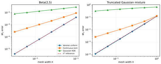
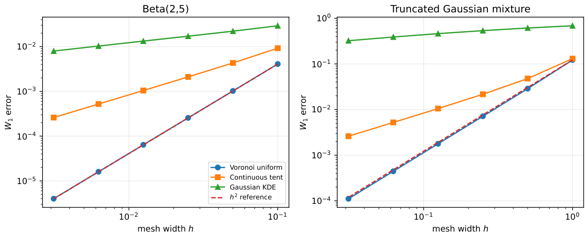
We bin two compactly supported continuous distributions on increasingly fine equal grids and provide the dequantizers with the exact cell masses. This isolates reconstruction from sampling noise. The first truth is Beta$(2,5)$ on $[0,1]$; the second is a two-component Gaussian mixture truncated to $[-5,5]$. We compare maximum-entropy Voronoi uniform dequantization, the continuous tent variant, and a weighted Gaussian KDE with Silverman bandwidth. The uniform method yields slopes of $1.999$ and $2.017$, essentially the theoretical value 2. The tent method is about first order in these experiments, while the KDE bandwidth decreases too slowly relative to the deterministic mesh. Table 1 reports the fitted convergence slopes, while Figure 1 shows the full error curves.

Table 1. Empirical slope of $\log W_1$ against $\log h$. The Voronoi-uniform slopes agree with the sharp $h^2$ theorem.

Ground Truth	Uniform	Tent	KDE
Beta(2,5)	1.999	1.025	0.373
Truncated Gaussian mixture	2.017	1.110	0.218

Figure 1. 1-Wasserstein distance ($W_1$) reconstruction error under deterministic mesh refinement. The left panel shows the Beta$(2,5)$ distribution, and the right panel shows the truncated Gaussian mixture. Blue circles represent Voronoi-uniform dequantization, orange squares represent the continuous tent kernel, and green triangles represent Gaussian kernel density estimation (KDE). The red dashed line indicates the theoretical $h^2$ reference rate. Both axes use logarithmic scales.

6.2. Multi-Scale Non-Uniform Support

We next use 12 support points with local spacings $0.2$, $0.5$, and 5. We measure (i) total variation between the original PMF and the PMF induced by nearest-neighbour requantization on the full line, (ii) the analytic mismatch probability ${ϵ}_p$ in Proposition 1, (iii) probability mass placed outside the finite mirrored dequantization domain, and (iv) the fraction of that domain on which the density is positive. In addition to global-width baselines, we include a stronger inscribed local uniform baseline: each atom receives the largest symmetric interval centered at $x_i$ that stays inside its own Voronoi cell. It therefore preserves the PMF exactly, but leaves gaps. Table 2 summarizes the resulting requantization error, mismatch probability, outside-domain mass, and domain coverage across the competing relaxations.

Table 2. Multi-scale support. The analytic mismatch probability $ϵ$ upper-bounds the observed requantized TV as predicted by Proposition 1. Exact right-inverse methods have both quantities equal to zero.

Method	Requantized TV	Mismatch $\mathit{ϵ}$	Outside Mass	Coverage
Voronoi uniform	0.0000	0.0000	0.0000	100.0%
Continuous tent	0.0000	0.0000	0.0000	100.0%
Inscribed local uniform	0.0000	0.0000	0.0000	52.8%
Fixed uniform $w=0.2$	0.0000	0.0000	0.0000	5.6%
Fixed uniform $w=1$	0.0255	0.2894	0.0383	17.4%
Fixed uniform $w=5$	0.2128	0.3983	0.1277	69.0%
Gaussian KDE	0.3110	0.7641	0.2663	100.0%

The experiment makes three points. First, exact recovery is not unique: any kernel confined to the assigned cell has it. Second, every approximate baseline satisfies the predicted inequality $\mathrm{TV}\le {ϵ}_p$. Third, maximum-entropy Voronoi uniformity is distinguished by filling each cell completely with no width choice, whereas the inscribed local uniform baseline leaves substantial gaps.

6.3. Downstream Model Capacity: No Favorable K Selected Post Hoc

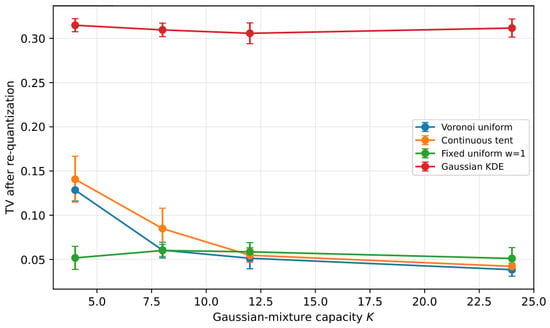
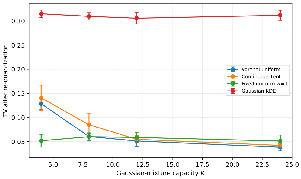
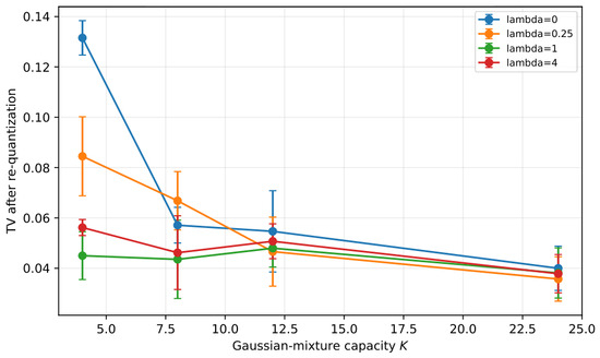
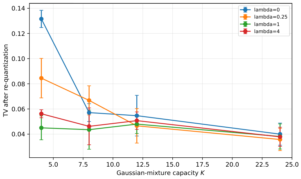
The original version of this project used one 24-component Gaussian mixture and, therefore, risked conflating relaxation quality with model capacity. We instead fit mixtures with $K\in \{4,8,12,24\}$, using ten random seeds per method/capacity combination. The training set contains 1200 dequantized draws and each fitted model is evaluated by requantizing 10,000 generated draws. Table 3 summarizes the resulting TV errors across model capacities, and Figure 2 visualizes the corresponding capacity sensitivity.

Table 3. Mean (SD) requantized TV error over ten seeds. Low capacity can favor smoother but biased relaxation; as capacity increases, the exact right-inverse relaxations become best.

K	Voronoi Uniform	Continuous Tent	Fixed Uniform w = 1	Gaussian KDE
4	0.128 (0.012)	0.141 (0.026)	0.052 (0.013)	0.315 (0.007)
8	0.061 (0.009)	0.085 (0.023)	0.060 (0.007)	0.310 (0.008)
12	0.051 (0.012)	0.055 (0.008)	0.059 (0.010)	0.306 (0.012)
24	0.038 (0.007)	0.042 (0.007)	0.051 (0.012)	0.312 (0.010)

Figure 2. Capacity sensitivity of the downstream Gaussian-mixture model. The horizontal axis shows the number of Gaussian-mixture components (K), and the vertical axis shows total variation (TV) error after requantization. Blue, orange, green, and red lines represent Voronoi-uniform dequantization, continuous tent dequantization, fixed-width uniform dequantization ($w=1$), and Gaussian kernel density estimation (KDE), respectively. Circular markers indicate mean TV errors, and error bars represent standard deviations across ten random seeds. The ordering changes at low K, demonstrating the importance of reporting downstream model capacity.

At $K=4$, fixed $w=1$ noise is easiest for the low-capacity smooth mixture to fit even though it is not probability preserving. At $K=24$, Voronoi uniform has a mean TV of $0.038$ compared with $0.051$ for fixed-width dequantization and roughly $0.312$ for KDE. The result is more informative than a single favorable capacity: exact representation and downstream approximation are separate design criteria.

6.4. Model-Aware Exact Kernels and the KL Decomposition

The capacity reversal above suggests that maximum entropy need not be the easiest exact representation for a restricted smooth model. We therefore apply Theorem 7 on the same 12-point support with $c_i\left(y\right)={\{(y-x_i)/0.5\}}^2$ and $\lambda \in \{0,0.25,1,4\}$. Every value is an exact right inverse; only the within-cell concentration changes. For each $K\in \{4,8,12,24\}$, we again fit ten independent Gaussian mixtures and evaluate requantized TV on generated draws. Table 4 reports the capacity-specific performance of the exact Gibbs family, and Figure 3 displays the corresponding model-aware concentration patterns.

Table 4. Mean (SD) requantized TV for the exact Gibbs family. The optimal concentration depends on downstream capacity, even though every column is exactly information preserving before approximation.

K	$\mathit{\lambda }=0$	$\mathit{\lambda }=0.25$	$\mathit{\lambda }=1$	$\mathit{\lambda }=4$
4	0.132 (0.007)	0.084 (0.016)	0.045 (0.010)	0.056 (0.003)
8	0.057 (0.007)	0.067 (0.012)	0.044 (0.016)	0.046 (0.015)
12	0.055 (0.016)	0.047 (0.014)	0.048 (0.007)	0.051 (0.007)
24	0.040 (0.009)	0.036 (0.009)	0.038 (0.010)	0.038 (0.008)

Figure 3. Model-aware exact dequantization. All curves use the same cells and preserve the target PMF exactly before the Gaussian-mixture approximation; only the within-cell Gibbs concentration changes.

At $K=4$, moving from the maximum-entropy endpoint $\lambda =0$ to $\lambda =1$ reduces mean TV from about $0.132$ to $0.045$; excessive concentration at $\lambda =4$ is slightly worse. At $K=24$, a milder $\lambda =0.25$ is best among the tested exact kernels, with mean TV about $0.036$. The preferred kernel therefore changes with approximation capacity rather than being universally uniform or maximally concentrated.

The same experiment also audits Theorem 4. For an eight-component fit to the $\lambda =0$ target, continuous KL equals categorical KL plus the weighted within-cell KL to numerical quadrature precision; Table 5 reports this numerical decomposition.

Table 5. Numerical audit of the exact downstream KL decomposition.

Quantity	Value
Continuous KL	0.045628
Categorical KL	0.015575
Within-cell KL	0.030053
Sum of terms	0.045628
Absolute identity error	6.94 $\times {10}^{-17}$

The decomposition exposes why continuous NLL alone can be a misleading proxy for discrete fidelity: part of the fitting budget is spent matching within-cell shape, which disappears after requantization.

• Geometric-scale reparameterization.

We examined $s_c\in \{0.25,0.5,1,2\}$. Because the kernel depends on the parameters only through the effective concentration

$$\alpha =\lambda /s_c^2,$$

parameter pairs yielding the same value of $\alpha$ are mathematically equivalent. For example, $\alpha =4$ is represented by

$$(\lambda ,s_c)=(0.25,0.25),(1,0.5),(4,1),(16,2).$$

Table 6 confirms this equivalence numerically on the multiscale support, with a maximum density difference of zero to machine precision. Thus, $\lambda$ and $s_c$ are not separately identifiable from the kernel, and there is no unique optimal $(\lambda ,s_c)$ pair. If the optimal effective concentration is ${\alpha }^{*}$, then the corresponding parameterization satisfies   

$${\lambda }^{*}\left(s_c\right)={\alpha }^{*}{s}_c^2.$$

Table 6. Scale reparameterization audit. Pairs with the same $\alpha =\lambda /s_c^2$ define the same exact Gibbs kernel, so $s_c$ changes the numerical labeling of concentration rather than adding an independent tuning dimension.

$\mathit{\alpha }=\mathit{\lambda }/{\mathit{s}}_{\mathit{c}}^2$	${\mathit{s}}_{\mathit{c}}$	Equivalent $\mathit{\lambda }$	Max. Density Difference
1	0.25	0.0625	0.0
1	0.50	0.25	0.0
1	1.00	1	0.0
1	2.00	4	0.0
4	0.25	0.25	0.0
4	0.50	1	0.0
4	1.00	4	0.0
4	2.00	16	0.0
16	0.25	1	0.0
16	0.50	4	0.0
16	1.00	16	0.0
16	2.00	64	0.0

For example, at $s_c=0.5$, the Gaussian-mixture optima are $\lambda =1$ for $K=4,8$ and $\lambda =0.25$ for $K=12,24$, corresponding to effective concentrations $\alpha =4$ and $\alpha =1$, respectively.

6.5. Rational-Quadratic Spline-Flow Validation and Finite-Sample Selection

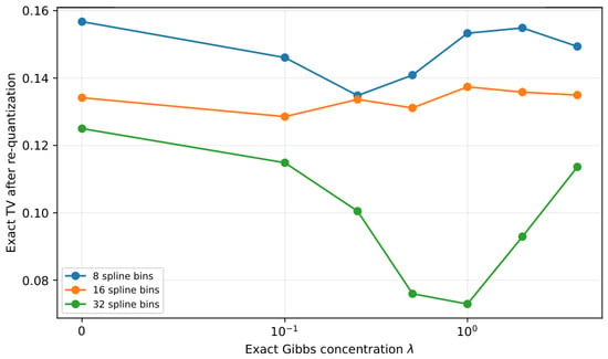
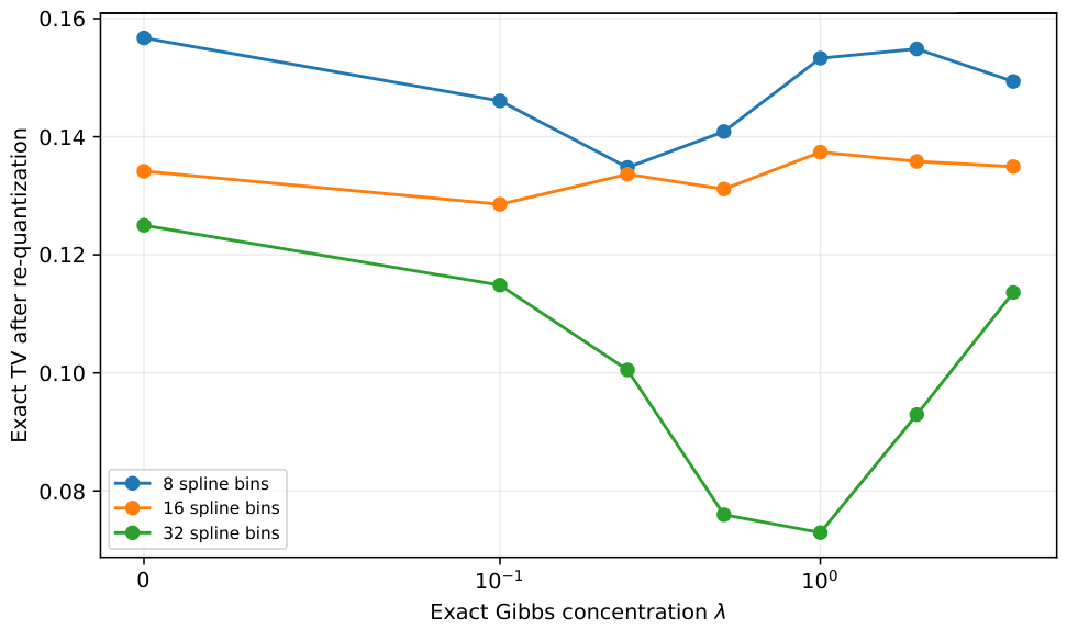
The Gaussian-mixture experiment deliberately varies a classical finite-capacity density family. We next ask whether the same model-aware effect persists for a modern invertible density model. We fit one-dimensional monotone rational-quadratic spline normalizing flows [21] on the same bounded dequantization domain. The implementation uses a uniform base on $[0,1]$, followed by an analytically invertible rational-quadratic spline and an affine map to the dequantization interval; hence, likelihoods, CDF values, sampling, and induced cell probabilities are all available exactly. Flow capacities use 8, 16, or 32 spline bins. For every capacity and seed, the same underlying discrete training sample is used across $\lambda \in \{0,0.1,0.25,0.5,1,2,4\}$; only the exact within-cell dequantization changes. Five seeds are used per capacity–concentration pair. Table 7 summarizes the exact requantized TV errors across flow capacities and Gibbs concentrations, while Figure 4 visualizes the corresponding capacity-dependent pattern.

Table 7. Mean exact requantized TV for rational-quadratic spline flows. The best exact Gibbs concentration changes with flow capacity; at 32 spline bins, $\lambda =1$ reduces the mean TV from $0.125$ at the uniform endpoint to $0.073$.

Flow Bins	$\mathit{\lambda }=0$	$\mathit{\lambda }=0.1$	$\mathit{\lambda }=0.25$	$\mathit{\lambda }=0.5$	$\mathit{\lambda }=1$	$\mathit{\lambda }=2$	$\mathit{\lambda }=4$
8	0.157	0.146	0.135	0.141	0.153	0.155	0.149
16	0.134	0.129	0.134	0.131	0.137	0.136	0.135
32	0.125	0.115	0.101	0.076	0.073	0.093	0.114

Figure 4. Model-aware exact dequantization with a rational-quadratic spline flow. Each target kernel is an exact right inverse before downstream fitting; the plotted error is introduced only by the fitted flow.

The flow experiment reinforces two conclusions. First, uniform dequantization is not uniformly easiest to approximate: the mean TV optimum is $\lambda =0.25$ with 8 spline bins, $\lambda =0.1$ with 16 bins, and $\lambda =1$ with 32 bins. Second, selecting the representation by continuous fit error need not select the representation with the best categorical fidelity. Across the 15 capacity–seed fits, the $\lambda$ minimizing Monte Carlo continuous KL and the $\lambda$ minimizing exact requantized TV disagree in 14 cases. This is the behavior predicted by Theorem 4: continuous KL includes the within-cell approximation term, whereas the downstream categorical target does not.

For black-box models whose cell probabilities cannot be integrated exactly, Algorithm 1 uses generated samples to estimate categorical risk. Table 8 audits Theorem 5 by repeatedly selecting among the seven fitted Gibbs candidates using m requantized generated draws per candidate. The corrected theorem has the required $m^{-1/2}$ Monte Carlo order. Its bound is intentionally distribution-free and conservative, but empirical regret decreases rapidly with the Monte Carlo budget even when the exact oracle candidate is not selected.

Algorithm 1 Model-aware exact dequantization

Given a fixed partition, target weights p, a finite tuning set $\Lambda$, and a downstream model class $\mathcal{F}$: (i) for each $\lambda \in \Lambda$, generate training data from the exact kernel $k_{\lambda }$ and fit ${\widehat{q}}_{\lambda ,\mathcal{F}}$; (ii) compute the induced categorical law $Q_{\#}{\widehat{q}}_{\lambda ,\mathcal{F}}$ exactly when cell probabilities are available, or estimate it by generating from ${\widehat{q}}_{\lambda ,\mathcal{F}}$ and requantizing; (iii) select the $\lambda$ minimizing a categorical loss such as TV or KL; and (iv) optionally refit the chosen continuous model using all available simulation/training budget. The selection criterion is deliberately categorical: Theorem 4 shows that continuous fit error contains a within-cell term that disappears after requantization. When p is estimated from observations rather than specified externally, the candidate fitting and tuning steps should use data splitting or cross-fitting so that the same observations do not determine both the plug-in target and its reported out-of-sample performance.

Table 8. Monte Carlo model-aware selection for the fitted spline flows. “Oracle hit” is the frequency of selecting the exact-TV best candidate; regret is measured in true requantized TV. The final column is the finite-sample bound in (5) at $\delta =0.05$.

Bins	m	Oracle Hit	Mean Regret	Max Regret	Bound
8	250	0.268	0.0092	0.0640	0.409
8	1000	0.416	0.0052	0.0330	0.204
8	5000	0.604	0.0021	0.0187	0.091
16	250	0.234	0.0073	0.0238	0.409
16	1000	0.347	0.0052	0.0238	0.204
16	5000	0.545	0.0022	0.0238	0.091
32	250	0.336	0.0065	0.0768	0.409
32	1000	0.446	0.0031	0.0237	0.204
32	5000	0.590	0.0014	0.0145	0.091

6.6. Geometry Perturbation Audit

To test Proposition 2, we perturb each site of the multiscale support independently by at most $\delta$, preserve the ordering, generate from the original Voronoi-uniform cells, and decode with the perturbed nearest-neighbor quantizer. Each row averages 200 perturbations. Table 9 compares the observed requantized TV, category-mismatch probability, and deterministic perturbation bound.

Table 9. Sensitivity to perturbed support geometry. Requantized TV is below the actual category-mismatch probability, which is itself below the deterministic bound in (6).

$\mathit{\delta }$	Mean TV	Max TV	Mean Mismatch	Deterministic Bound
0.00	0.0000	0.0000	0.0000	0.0000
0.01	0.0030	0.0061	0.0045	0.0313
0.02	0.0063	0.0123	0.0093	0.0626
0.04	0.0127	0.0281	0.0192	0.1252
0.08	0.0250	0.0489	0.0371	0.2504

The bound is intentionally conservative but monotone and fully deterministic once p, the cell widths, and a site-error radius are specified. This provides a simple audit when support locations or embeddings are estimated rather than known exactly.

6.7. Real Irregular Support: Wine Proline Measurements

The scikit-learn Wine dataset (scikit-learn; https://scikit-learn.org/; accessed on 20 September 2026) contains 178 observations and is distributed with the package. We use the empirical distribution of its “proline” feature: 121 distinct observed values, with adjacent gaps ranging from 1 to 133 and a median gap of $7.5$. Treating the empirical mass function as the specified discrete target produces a real irregular-spacing example without inventing a synthetic geometry. The exact dequantization statements are conditional on these empirical weights; they do not remove the sampling uncertainty involved in estimating the population PMF from 178 observations. Table 10 reports the resulting category-mismatch and requantization diagnostics for this irregular-support example.

Table 10. Wine proline empirical PMF. The mismatch probability $ϵ$ controls the requantized TV error; exact Voronoi/tent kernels have $ϵ=0$.

Method	Requantized TV	Mismatch $\mathit{ϵ}$	Outside Mass	Coverage
Voronoi uniform	0.0000	0.0000	0.0000	100.0%
Continuous tent	0.0000	0.0000	0.0000	99.6%
Inscribed local uniform	0.0000	0.0000	0.0000	67.2%
Fixed uniform w = 7.5	0.0511	0.2103	0.0000	48.6%
Fixed uniform w = 10	0.0711	0.2913	0.0000	58.4%
Fixed uniform w = 50	0.2387	0.7979	0.0029	89.5%
Gaussian KDE	0.3045	0.9636	0.0497	100.0%

The exact methods have zero category mismatch by construction. For fixed-width and Gaussian relaxations, the analytic mismatch probability is reported beside the resulting requantized TV, making the coupling bound directly checkable on real irregular support. The outside-domain column is kept separate because leaving the finite mirrored plotting domain need not imply a category error after nearest-neighbor clipping. These metrics are not intended as a density-estimation contest: they measure faithfulness to the specified empirical discrete law.

6.8. Two Real Discrete-to-Continuous Distributional Applications

We finally evaluate the specific use case that motivates dequantization in practice: a genuinely discrete numeric variable is represented either by its original atoms or by an exact continuous relaxation, after which the same smooth downstream density model is fitted. We use two real datasets with meaningful numeric category geometry rather than arbitrary class codes. The UCI Abalone data contain 4177 specimens and an integer “Rings” variable, with ring count plus 1.5 used as an age proxy [22]. The RAND Health Insurance Experiment subset contains 20,190 observations; we use mdvis, the number of annual outpatient visits to a physician [23,24].

For each dataset, we fix the integer lattice over the published observed range and use its half-integer Voronoi cells. Five outer folds are used for evaluation; within each training fold, 20% of the remaining observations are reserved for selecting the exact Gibbs concentration $\lambda \in \{0,0.25,1,4\}$ by categorical validation NLL. Thus, the test observations are not used to estimate the training PMF, select the kernel, or fit the continuous model. Every continuous fit uses the same 32-bin rational-quadratic spline flow. The matched “raw discrete” comparator fits that flow directly to the integer atoms without dequantization. After fitting, flow probabilities are integrated exactly over the Voronoi cells, so all reported test criteria are again discrete: held-out categorical NLL and total variation from the held-out empirical PMF. A Jeffreys-smoothed categorical PMF is included as a direct discrete reference, not as a model we expect dequantization to dominate. Table 11 summarizes held-out NLL and TV across the five outer folds for both applications.

Table 11. Two real discrete-to-continuous applications. Entries are shown as the mean (SD across five held-out folds). The proposed continuous representation is compared with fitting the identical spline flow directly to the original atoms.

Dataset	Method	Test NLL	SD	Test TV	SD
Abalone rings	Categorical reference	2.505	0.038	0.065	0.010
Abalone rings	Raw discrete atoms + flow	2.558	0.045	0.140	0.020
Abalone rings	Voronoi-uniform + flow	2.508	0.037	0.068	0.009
Abalone rings	Selected exact dequantization + flow	2.506	0.038	0.065	0.010
RAND doctor visits	Categorical reference	2.180	0.023	0.030	0.006
RAND doctor visits	Raw discrete atoms + flow	2.237	0.032	0.091	0.013
RAND doctor visits	Voronoi-uniform + flow	2.191	0.022	0.046	0.009
RAND doctor visits	Selected exact dequantization + flow	2.189	0.022	0.044	0.013

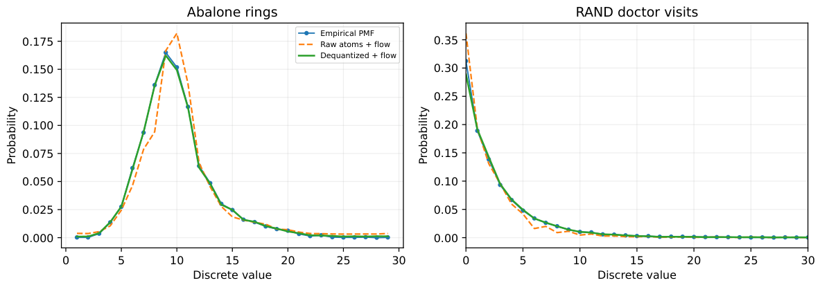
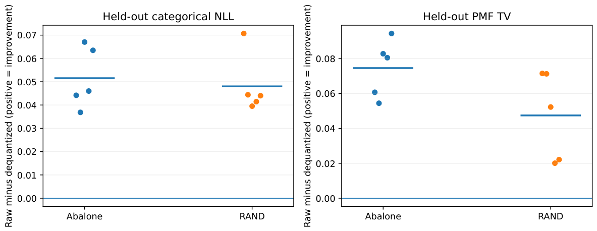
The representation effect is consistent in every fold. For Abalone rings, model-aware dequantization lowers mean held-out NLL from 2.558 to 2.506 and TV from 0.140 to 0.065; the dequantized flow wins all five folds on both criteria. For RAND physician visits, NLL falls from 2.237 to 2.189 and TV from 0.091 to 0.044, again with five of five fold-wise wins. Thus, the continuous relaxation cuts the PMF approximation error of the matched smooth flow by roughly one half in both applications. Uniform Voronoi dequantization already captures most of this gain, while validation-selected Gibbs concentration yields a small additional improvement.

The categorical reference is intentionally informative about what this result does not claim. In the Abalone data, the selected continuous flow essentially matches the direct categorical reference (NLL 2.506 versus 2.505; TV 0.065 versus 0.065), while in the much larger RAND sample the unrestricted categorical reference remains better. This is consistent with the Blackwell result: dequantization cannot create information. Its benefit is computational and representational—when a smooth continuous model is to be used, an exact cell-respecting relaxation is substantially easier to fit faithfully than the original atomic sample.

These results also clarify when the within-cell kernel can matter practically. The strongest evidence in the present experiments is for downstream capacity: the preferred effective concentration changes with Gaussian-mixture or spline-flow capacity, and the raw-atom singularity is especially difficult for a smooth finite-capacity density model. Irregular cell widths and highly uneven masses can make the continuous target more heterogeneous and may therefore magnify representation effects, but the present experiments do not isolate a monotone causal relationship with spacing irregularity or mass imbalance. We therefore avoid claiming such a law without a dedicated factorial study.

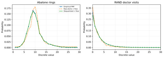
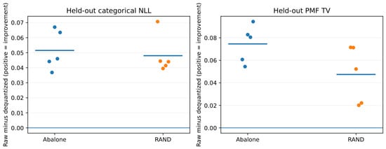
Figure 5 and Figure 6 show, respectively, the averaged PMF reconstructions and the fold-wise gains from exact dequantization relative to fitting the same spline flow directly to the atoms.

Figure 5. Real-data PMF reconstruction. Curves average the five outer-fold fits. Exact dequantization allows the same spline flow to track the discrete target substantially better than fitting the raw atoms directly. The RAND panel is shown through 30 visits for readability.

Figure 6. Fold-wise gain from transforming the discrete observations to the proposed exact continuous representation before fitting the spline flow. Positive values mean the dequantized representation has lower test error. All ten dataset–fold comparisons are positive for both NLL and TV.

6.9. Likelihood-Equivalence Audit

To verify the finite-sample likelihood statement in Theorem 2, we use a one-parameter softmax family on five irregular support points, draw one discrete sample of size 400, and dequantize that same sample with either the Voronoi-uniform or continuous-tent kernel. For each kernel we optimize the continuous likelihood and compare its centered likelihood curve with the original discrete likelihood. Table 12 reports the resulting agreement in MLEs and centered log-likelihood values.

Table 12. Numerical audit of likelihood preservation. The continuous likelihood differs from the discrete likelihood only by a parameter-free kernel term.

Kernel	Continuous MLE	$|{\widehat{\mathit{\theta }}}_{\mathit{Y}}-{\widehat{\mathit{\theta }}}_{\mathit{X}}|$	Max Centered Log-Likelihood Difference
Voronoi uniform	0.572007	1.89 $\times {10}^{-15}$	1.14 $\times {10}^{-13}$
Continuous tent	0.572007	8.56 $\times {10}^{-9}$	1.14 $\times {10}^{-13}$

The MLEs agree to numerical optimization tolerance, and the centered log-likelihood curves agree to floating-point precision. This experiment is intentionally simple: it checks the implementation of an exact algebraic identity rather than supplying evidence for an asymptotic claim.

6.10. Numerical Checks of Exact Identities and Multidimensional Mass

Table 13 numerically integrates three divergences for two random weight vectors on the same irregular support. Errors are below $3\times {10}^{-6}$ on a million-point integration grid, consistent with the exact identity in Theorem 3.

Table 13. Numerical verification of exact divergence preservation.

Divergence	Discrete	Dequantized	Absolute Error
Total variation	0.27879604	0.27879380	2.25 $\times {10}^{-6}$
KL divergence	0.39887339	0.39887418	7.99 $\times {10}^{-7}$
Squared Hellinger	0.08102905	0.08102833	7.23 $\times {10}^{-7}$

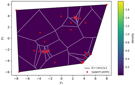
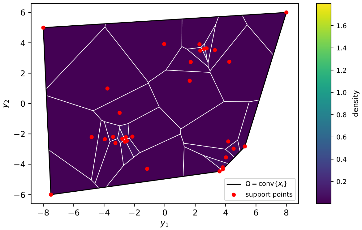
In two dimensions, we use $\Omega =\mathrm{conv}\left\{x_i\right\}$ for 31 irregular support points. The clipped Voronoi cells cover the convex hull to numerical precision (total area $148.1506935$), and ${\sum }_i(p_i/|C_i\left|\right)|C_i|=1$ to machine precision. Figure 7 shows the bounded-domain construction.

Figure 7. Two-dimensional weighted Voronoi dequantization on the explicit bounded domain $\Omega =\mathrm{conv}\left\{x_i\right\}$. The black outline marks the convex-hull boundary, the white lines delineate the internal Voronoi cells, red dots mark the support sites, and the color scale represents the density.

6.11. Estimated-Weight Plug-In Audit

Equation (3) is distribution-free. To illustrate its scale, Table 14 repeatedly estimates the 12-category synthetic PMF used in the model-aware experiments. The empirical TV decreases at the expected $N^{-1/2}$ rate, and the stated high-probability bound is conservative. By Equation (2), the same TV values apply exactly after dequantization with any common fixed cell-confined kernel.

Table 14. Finite-sample plug-in audit for an empirically estimated 12-category PMF (5000 repetitions). The final column is the fraction of repetitions satisfying the $1-\delta$ bound with $\delta =0.05$.

N	Mean TV	95th Pct. TV	Bound ($\mathit{\delta }=0.05$)	Empirical Coverage
100	0.1315	0.1832	0.2882	1.000
400	0.0657	0.0919	0.1441	1.000
1600	0.0327	0.0457	0.0721	1.000
6400	0.0165	0.0229	0.0360	1.000

6.12. Computational Scope of the Current Implementation

The closed-form one-dimensional construction is inexpensive because only adjacent support points are needed once the support is ordered. The present multidimensional implementation explicitly constructs a two-dimensional Voronoi diagram and clips its cells to the convex hull; that is, a computational-geometry implementation, not a claim that explicit clipped-cell enumeration remains practical in high dimension. Table 15 reports a machine-specific timing audit included for order-of-magnitude guidance rather than as a hardware-independent benchmark. In this environment, one-dimensional boundary construction remains negligible through ${10}^6$ support points, while the bounded two-dimensional implementation remains sub-second through 1000 support points. The reproducibility code does not implement explicit bounded-cell enumeration above two dimensions. In higher dimensions, Voronoi complexity can grow rapidly and practical use would require specialized polytope libraries, approximate/implicit nearest-neighbor representations, or sampling methods that avoid enumerating every cell.

Table 15. Implementation scaling audit (median of five runs). Times are machine-specific and are reported only to indicate the computational scope of the supplied code.

Dimension	Support Points	Median Time (s)	Max Time (s)
1D	1000	0.00001	0.00004
1D	10,000	0.00001	0.00008
1D	100,000	0.00009	0.00072
1D	1,000,000	0.00228	0.00761
2D bounded	25	0.00164	0.00435
2D bounded	50	0.00269	0.00304
2D bounded	100	0.00438	0.00489
2D bounded	250	0.00980	0.01002
2D bounded	500	0.01878	0.01972
2D bounded	1000	0.03715	0.05108

7. Discussion

The central formula in this paper overlaps with weighted Voronoi density constructions; pretending otherwise would weaken the contribution. The useful distinction is the object being represented. For density estimation, the cells arise from samples, and cell volume is used to estimate an unknown continuous density. Here, the finite weight vector is already the probability law of interest, and the continuous density is required to be an invertible relaxation under a specified quantizer.

This perspective yields several practical consequences. Exact requantization is guaranteed rather than assessed approximately. More strongly, Theorem 2 shows that when the parameter enters only through the discrete weights, dequantization preserves the entire statistical experiment before a downstream approximation is imposed. This is a statement about equivalence of statistical experiments, not a guarantee about an arbitrary model subsequently fitted to the continuous outputs. Theorem 4 identifies exactly where that later approximation error enters: categorical error and within-cell shape error add in KL when the fitted model covers the target cells. This resolves the apparent tension in the capacity experiments. Exact kernels carry the same discrete information, yet a restricted continuous model can approximate them very differently. The Gibbs family makes that representation choice explicit instead of treating uniform noise as inevitable. The spline-flow experiment shows that this is not peculiar to Gaussian mixtures: the preferred exact kernel changes with flow capacity, and continuous KL and categorical fidelity select different concentrations in 14 of 15 seed-wise comparisons. The finite-sample oracle inequality then makes the selection step operational even when the induced category probabilities of a fitted continuous model are available only by simulation. The two additional real-data studies in Section 6.8 show the same representation effect on natural count variables: under a matched spline-flow model, exact continuousization improves held-out requantized NLL and TV in every fold for both Abalone ring counts and RAND physician visits.

A related distinction appears in a recent stochastic-modeling study, where mechanistic model construction is evaluated separately from out-of-family numerical and stochastic verification [25]. Here, the analogous separation is between an exact information-preserving representation and the approximation properties of the continuous model fitted afterward.

The limitations are equally important. First, the geometric support itself must be meaningful; categorical labels with arbitrary numeric codes should not be assigned Euclidean Voronoi cells without a defensible embedding. Second, high-dimensional Voronoi construction can be expensive, as emphasized by the VDE literature [11,12]; the supplied implementation is deliberately closed-form in one dimension and explicit only in bounded two-dimensional geometry. Third, a bounded ambient domain is part of the multidimensional model. Fourth, the piecewise-uniform density is not differentiable at cell boundaries and has zero score within cells, so it should not be presented as a ready-made score model. Fifth, the finite KL decomposition requires downstream cell coverage; truncated models that leave target-positive regions uncovered yield infinite within-cell KL rather than a finite categorical/shape split. Finally, model-aware tuning is not free of design choices. If the weights are estimated from data, exactness is conditional on the plug-in vector, population error remains governed by $p-\widehat{p}$, and data splitting or cross-fitting is appropriate when kernel selection and downstream fitting are data-driven. If the weights themselves are an unknown parameter in an inferential model, allowing the kernel to depend on that parameter would invalidate the parameter-independent likelihood-preservation statement. Geometry-perturbation bounds also require a meaningful labeling correspondence between original and perturbed cells. The selector guarantee in Theorem 5 is conditional on the fitted downstream models and controls only Monte Carlo selection error; it is not a generalization bound for the training procedure itself.

8. Conclusions

We developed an information-preserving and model-aware theory for dequantizing weighted discrete laws on prescribed partitions. Exact cell-confined kernels are stochastic right inverses and produce a Blackwell-equivalent continuous experiment; inference and information are unchanged until a downstream approximation is imposed. At that point, an exact KL chain rule separates the discrete error that matters after requantization from within-cell shape error. This distinction leads to an entropy–transport Gibbs family of exact kernels: uniform dequantization is one endpoint, while concentration can be tuned to the capacity of the downstream model without sacrificing exact category recovery. Leakage and geometry-perturbation bounds quantify departures from the ideal construction, and Voronoi geometry supplies exact transport costs and a sharp $\Theta \left(h^2\right)$ reconstruction result. A finite-sample selector provides an oracle guarantee for choosing among candidate exact kernels when categorical masses are estimated by simulation, and rational-quadratic spline-flow experiments confirm that the capacity-aware effect survives beyond Gaussian mixtures. Two real count-data applications further show that, when the same smooth flow is mandated, exact continuousization can reduce requantized PMF error by roughly one half relative to fitting that flow directly to the original atoms. The unrestricted categorical reference matches or outperforms the dequantized pipeline, as expected: the contribution is an information-preserving continuous representation for continuous-model workflows, not a replacement for direct categorical modeling. The resulting framework shifts the question from “which noise is convenient?” to “which information-preserving continuous representation is easiest for the model class that will actually be used?”

References

- Uria, B.; Murray, I.; Larochelle, H. RNADE: The real-valued neural autoregressive density-estimator. In Advances in Neural Information Processing Systems 26; Curran Associates, Inc.: Red Hook, NY, USA, 2013; Available online: https://proceedings.neurips.cc/paper/2013/hash/53adaf494dc89ef7196d73636eb2451b-Abstract.html (accessed on 20 September 2026).
- Theis, L.; van den Oord, A.; Bethge, M. A Note on the Evaluation of Generative Models. In Proceedings of the International Conference on Learning Representations, San Juan, Puerto Rico, 2–4 May 2016; Available online: https://arxiv.org/abs/1511.01844 (accessed on 20 September 2026).
- Dinh, L.; Sohl-Dickstein, J.; Bengio, S. Density Estimation Using Real NVP. In Proceedings of the International Conference on Learning Representations, Toulon, France, 24–26 April 2017; Available online: https://openreview.net/forum?id=HkpbnH9lx (accessed on 20 September 2026).
- Ho, J.; Chen, X.; Srinivas, A.; Duan, Y.; Abbeel, P. Flow++: Improving Flow-Based Generative Models with Variational Dequantization and Architecture Design. In Proceedings of the International Conference on Machine Learning, Long Beach, CA, USA, 9–15 June 2019; Volume 97. Available online: https://proceedings.mlr.press/v97/ho19a.html (accessed on 20 September 2026).
- Hoogeboom, E.; Cohen, T.S.; Tomczak, J.M. Learning Discrete Distributions by Dequantization. arXiv 2020, arXiv:2001.11235. [Google Scholar] [CrossRef] [Scilit]
- Gad, K.A.E.; Atia, F.A.; Abouelenein, M.F.; Hamouda, H.M.; Moussa, M.; Elshafae, S. Conformable Calculus Derivation of the Power Function Distribution: Reparameterization and Applications. Next Mater. 2026, 13, 102790. [Google Scholar] [CrossRef] [Scilit]
- Gad, K.A.E.; Atia, F.A.; Moussa, M.; Hamouda, H.M.; Abouelenein, M.F.; Abdul-Moniem, I.B.; Eldeeb, A.S. The Fractional Exponential Distribution: A Gamma Subfamily from Conformable Calculus. Results Eng. 2026, 31, 111224. [Google Scholar] [CrossRef] [Scilit]
- Gad, K.A.E.; Atia, F.A.; Moussa, M.; Abouelenein, M.F.; Hamouda, H.M.; Abdul-Moniem, I.B.; Eldeeb, A.S. The Exponentiated New Failure Distribution: Theory and Applications. Results Eng. 2026, 32, 111907. [Google Scholar] [CrossRef] [Scilit]
- Duah, K.; Sun, Y.; Moussa, M. A Random Quantile Approach for Prior Covariance Estimation in Bayesian Maximum Entropy. Spat. Stat. 2026, 73, 100974. [Google Scholar] [CrossRef] [Scilit]
- Grzegorzewski, P.; Moussa, M.; Sun, Y.; Elshafae, S. Uncertainty-Aware Repeated-Measures ANOVA for Interval-Valued Data with an Application to Longitudinal CT Tumor Imaging. In Information Processing and Management of Uncertainty in Knowledge-Based Systems; Communications in Computer and Information Science; Springer: Cham, Switzerland, 2026; Volume 3019, pp. 477–491. [Google Scholar] [CrossRef] [Scilit]
- Polianskii, V.; Marchetti, G.L.; Kravberg, A.; Varava, A.; Pokorny, F.T.; Kragic, D. Voronoi Density Estimator for High-Dimensional Data: Computation, Compactification and Convergence. In Proceedings of the Conference on Uncertainty in Artificial Intelligence, Eindhoven, The Netherlands, 2–4 August 2022; Volume 180, pp. 1644–1653. Available online: https://proceedings.mlr.press/v180/polianskii22a.html (accessed on 20 September 2026).
- Marchetti, G.L.; Polianskii, V.; Varava, A.; Pokorny, F.T.; Kragic, D. An Efficient and Continuous Voronoi Density Estimator. In Proceedings of the International Conference on Artificial Intelligence and Statistics, Valencia, Spain, 25–27 April 2023; Volume 206, pp. 4732–4744. Available online: https://proceedings.mlr.press/v206/marchetti23a.html (accessed on 20 September 2026).
- Chen, R.T.Q.; Amos, B.; Nickel, M. Semi-Discrete Normalizing Flows through Differentiable Tessellation. In Advances in Neural Information Processing Systems; Curran Associates, Inc.: Red Hook, NY, USA, 2022; Volume 35. [Google Scholar] [CrossRef] [Scilit]
- Blackwell, D. Comparison of Experiments. In Proceedings of the Second Berkeley Symposium on Mathematical Statistics and Probability, Berkeley, CA, USA, 31 July–12 August 1950; pp. 93–102. Available online: https://projecteuclid.org/euclid.bsmsp/120050022 (accessed on 20 September 2026).
- Blackwell, D. Equivalent Comparisons of Experiments. Ann. Math. Stat. 1953, 24, 265–272. [Google Scholar] [CrossRef] [Scilit]
- Moussa, M.; Ratterman, C.; Zhang, W.; Zhe, S.; Sun, Y. DeepCut: Adaptive Neural Network Thresholds for Precipitation Phase Partitioning. Mach. Learn. Earth 2026, 2, 015009. [Google Scholar] [CrossRef] [Scilit]
- Moussa, M. Auditing Conformal Prediction under Distribution Shift: A Detectability Boundary, Exact Label-Budget Design, and Repair. Res. Sq. 2026. [Google Scholar] [CrossRef] [Scilit] [PubMed]
- Moussa, M.A.; Gad, K.A.E.; Sharabati, W.K.; Hamouda, H.M. Risk-Guided Maintenance of Sports AI Under Seasonal Shift: Empirical-Bayes Recalibration with Anytime-Valid Certification. Preprints 2026. [Google Scholar] [CrossRef] [Scilit]
- Nielsen, D.; Winther, O. Closing the Dequantization Gap: PixelCNN as a Single-Layer Flow. In Advances in Neural Information Processing Systems; Curran Associates, Inc.: Red Hook, NY, USA, 2020; Volume 33, Available online: https://proceedings.neurips.cc/paper/2020/hash/4c5bcfec8584af0d967f1ab10179ca4b-Abstract.html (accessed on 20 September 2026).
- Tan, S.; Huang, C.W.; Sordoni, A.; Courville, A. Learning to Dequantise with Truncated Flows. In Proceedings of the International Conference on Learning Representations, Virtual Event, 25–29 April 2022; Available online: https://openreview.net/forum?id=fExcSKdDo_ (accessed on 20 September 2026).
- Durkan, C.; Bekasov, A.; Murray, I.; Papamakarios, G. Neural Spline Flows. In Advances in Neural Information Processing Systems; Curran Associates, Inc.: Red Hook, NY, USA, 2019; Volume 32, Available online: https://proceedings.neurips.cc/paper/2019/hash/7ac71d433f282034e088473244df8c02-Abstract.html (accessed on 20 September 2026).
- Nash, W.; Sellers, T.; Talbot, S.; Cawthorn, A.; Ford, W. Abalone. Dataset, UCI Machine Learning Repository. 1994. Available online: https://archive.ics.uci.edu/dataset/1/abalone (accessed on 20 September 2026).
- Cameron, A.C.; Trivedi, P.K. Microeconometrics: Methods and Applications; Cambridge University Press: Cambridge, UK, 2005. [Google Scholar] [CrossRef] [Scilit]
- Seabold, S.; Perktold, J. Statsmodels: Econometric and Statistical Modeling with Python. In Proceedings of the 9th Python in Science Conference, Austin, TX, USA, 28 June–3 July 2010; pp. 92–96. Available online: https://conference.scipy.org/proceedings/scipy2010/seabold.html (accessed on 20 September 2026).
- Moussa, M.; Youssef, S.; Elrayany, K.; Nafea, A. Mechanism-Resolved Fractional–Volterra Modeling for Thermal-Hazard Screening: Lithium-Ion Battery Intervention Evidence, PDE Transfer, and Stochastic Verification. SSRN Preprint, 2026. SSRN 7322883. Available online: https://papers.ssrn.com/sol3/papers.cfm?abstract_id=7322883 (accessed on 20 September 2026).
Disclaimer/Publisher’s Note: The statements, opinions and data contained in all publications are solely those of the individual author(s) and contributor(s) and not of MDPI and/or the editor(s). MDPI and/or the editor(s) disclaim responsibility for any injury to people or property resulting from any ideas, methods, instructions or products referred to in the content. |
© 2026 by the authors. Licensee MDPI, Basel, Switzerland. This article is an open access article distributed under the terms and conditions of the Creative Commons Attribution (CC BY) license.