


Abstract
Generative probabilistic models differ in a fundamental way that is rarely measured directly: some permit exact inference, while others are more expressive but require their likelihood to be estimated. This study compares three model families on binarized Fashion-MNIST and MNIST under identical preprocessing, identical data splits, and matched parameter counts, evaluating every model by test log-likelihood on a common scale. Sum-product networks and mixtures of Bernoullis return exact likelihoods; the likelihood of a restricted Boltzmann machine is obtained by annealed importance sampling and reported with the effective sample size of the importance weights and a convergence study. Three results follow. First, the structure of a sum-product network matters more than its size: changing only which pixels are assigned to which leaf region, at a fixed parameter count of 706,800, is worth 38.7 nats on Fashion-MNIST and 41.2 nats on MNIST, whereas multiplying the capacity of a flat mixture eightfold yields approximately 13 nats. A network whose regions are misaligned with the data performs worse than a model with no hierarchy at all. Second, once the regions are aligned, the benefit of hierarchy depends on the data: the network exceeds the best flat mixture by 17.2 nats on Fashion-MNIST but falls 2.0 nats short on MNIST, where whole-image prototypes already suffice. Third, the restricted Boltzmann machine outperforms every tractable model tested at matched capacity, leading the best of them by 11.4 nats on Fashion-MNIST and 46.1 nats on MNIST, which quantifies the cost of guaranteeing exact inference. Exact inference nonetheless carries a practical benefit: for image completion, the sum-product network computes conditional marginals exactly and improves on max-product in every configuration tested. Training a fully connected Boltzmann machine to convergence proved infeasible on the available hardware, and the computational limitations are reported quantitatively.
1. Introduction
Generative modelling has become a central area of machine learning because of its ability to represent the distribution underlying a dataset rather than only the boundaries between classes. Where a discriminative model estimates , a generative model estimates , or the joint distribution , which makes tasks such as image synthesis, anomaly detection, data imputation and probabilistic reasoning available from a single learned object [1].
Among the various approaches, energy-based models represent data through an energy function in which lower-energy configurations are assigned higher probability. The idea traces to statistical mechanics and to early neural network models such as the Hopfield network [2], and led to the introduction of Boltzmann machines [3,4], which provided a probabilistic framework for modelling complex distributions over binary variables. Restricted Boltzmann machines followed as a simplified variant in which connections within a layer are removed [4]. That restriction makes the hidden units conditionally independent given the visible units, which in turn makes Gibbs sampling and contrastive divergence training practical, and it is the reason the restricted form rather than the general one became widely used in feature learning, dimensionality reduction and the construction of deep architectures [5,6].
Energy-based models share a structural difficulty. Their probabilities are defined only up to a normalizing constant, the partition function, whose exact evaluation requires summing over every configuration of the variables and is therefore intractable for models of realistic size [7]. A likelihood cannot be reported without it. Annealed importance sampling [8] provides a practical estimator by bridging from a tractable distribution to the target through a sequence of intermediate distributions, but it returns an estimate rather than an exact value, and one whose reliability depends on how well the sampling chains mix.
A separate line of work approaches the same problem from the opposite direction. Rather than accepting an intractable partition function and estimating it, tractable probabilistic models restrict the model class so that exact inference is guaranteed by construction. Sum-product networks [9] are the most prominent example: a rooted directed acyclic graph of sum and product nodes over tractable leaf distributions, in which any marginal or conditional probability can be computed exactly in time linear in the size of the network, provided the network satisfies simple structural conditions [10,11]. The partition function, which is the obstacle for energy-based models, becomes a single forward pass.
This difference raises an empirical question that is easy to state and rarely answered directly. Exact inference is clearly desirable, but it is obtained by restricting the model class, and a restriction has a cost. How large is that cost, measured on the same data, at the same parameter count, on the same scale? Answering it requires more care than a table of numbers from separate papers can provide, since likelihood values depend on preprocessing, on data splits, and on whether the reported figure is exact or estimated.
A second question concerns sum-product networks specifically. Their tractability follows from the structure of the network, and that structure must be chosen before training: the variables are partitioned into regions, and product nodes assert independence between them. The literature on structure learning is largely concerned with searching this space efficiently [11,12]. Much less attention has been given to what happens when the chosen structure is simply wrong for the data, even though every application must make that choice.
This study addresses both questions. Sum-product networks, mixtures of Bernoullis and restricted Boltzmann machines are trained on binarized Fashion-MNIST and MNIST under identical preprocessing, identical data splits and matched parameter counts, and evaluated by test log-likelihood, image completion and reconstruction. Two sum-product networks are compared that are identical in every respect except how variables are assigned to leaf regions, isolating the contribution of the structure from that of capacity. Likelihoods for the restricted Boltzmann machine are estimated by annealed importance sampling and reported alongside the diagnostics needed to judge them. A fully connected Boltzmann machine is also examined, though its training cost places a likelihood evaluation beyond the compute available; the reasons are reported quantitatively rather than asserted.
The contributions of this work are summarized as follows:
- We provide a unified empirical comparison of sum-product networks, mixtures of Bernoullis and restricted Boltzmann machines under identical preprocessing, identical data splits and matched parameter counts on both Fashion-MNIST and MNIST, allowing model families that are typically studied in isolation to be compared directly. Every reported likelihood is labelled as exact or estimated, so that values obtained under different guarantees are not conflated.
- We isolate the contribution of hierarchical structure from that of capacity by comparing two sum-product networks that differ only in how variables are assigned to leaf regions, holding parameter count, node counts, depth, optimizer, learning rate and random seed fixed. This shows that a hierarchy misaligned with the data performs worse than a model with no hierarchy at all, and that the benefit of an aligned hierarchy depends on the dataset rather than being a property of the model alone.
- We quantify the cost of tractable inference by comparing models whose likelihoods are exact against an energy-based model whose likelihood must be estimated, at matched capacity on both datasets, and document the practical benefit that exact inference confers on conditional queries: for image completion the network computes conditional marginals exactly and improves on max-product in every configuration tested.
- We report test log-likelihood for the restricted Boltzmann machine together with a convergence study of the annealed importance sampling estimator, varying the annealing schedule, the number of chains and the number of Gibbs sweeps, and reporting the effective sample size of the importance weights throughout. This establishes that the reduced effective sample size on the trained models reflects the difficulty of the target distribution rather than the estimator, and identifies which of the two levers actually improves it.
- We report complete training specifications, runtimes and diagnostic measurements for every model, including the relative magnitude of the learned lateral weights of a Boltzmann machine, which accounts for the proximity of its performance to that of the restricted architecture and explains why a comparable evaluation of the full model lies beyond the compute available.
The remainder of the paper is organized as follows. Section 2 reviews energy-based models, the estimation of partition functions and sum-product networks, consolidating both families into a common notation. Section 3 describes the datasets and the experimental protocol; Section 4 reports the results; Section 5 discusses their interpretation; Section 6 states the limitations and directions for future work, and Section 7 concludes.
2. Materials and Methods
2.1. Energy-Based Models
Energy-based models (EBMs) are a class of probabilistic generative models that represent data through an energy function, where lower-energy configurations correspond to higher probabilities. Unlike conventional probabilistic approaches, EBMs model complex dependencies by assigning energy values to different data states and deriving probabilities from these energy functions [1].
The probability of a configuration x is defined in terms of its energy as follows:
Taking the logarithm of both sides yields
where denotes the log-likelihood of configuration x, and Z is the partition function that normalizes the probability distribution. Maximizing the log-likelihood increases the probability assigned to observed data while accounting for the normalization term log Z.
This formulation implies that configurations with lower energy values are assigned higher probabilities, while configurations with higher energy values are less likely to occur. This energy-based framework forms the foundation of Boltzmann machines and restricted Boltzmann machines [3,4].
2.1.1. Boltzmann Machines
Boltzmann machines (BMs) are energy-based probabilistic graphical models that learn complex probability distributions from binary-valued data. As members of the Markov random field (MRF) family, BMs consist of visible and hidden units connected through weighted undirected links. The model associates each network configuration with an energy value, where lower-energy configurations correspond to higher probabilities. This energy-based framework enables BMs to capture dependencies among variables and learn underlying patterns from observed data.
A distinctive feature of a BM is its fully connected architecture, allowing each unit to interact with every other unit in the network. While this connectivity provides considerable representational power, it also introduces significant computational challenges. In particular, learning and inference require computation of the partition function, whose complexity grows exponentially with the number of units, making exact training computationally intractable for large networks [7].
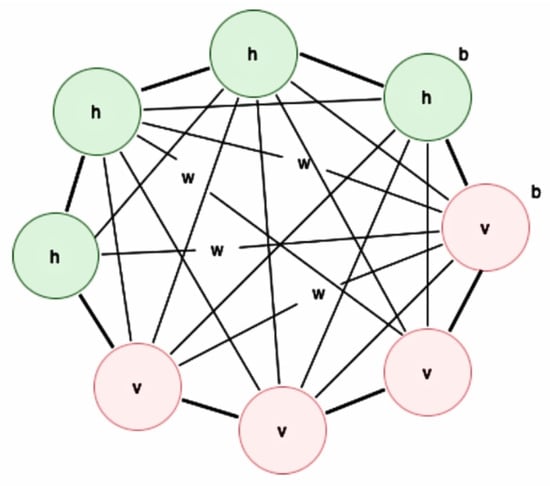
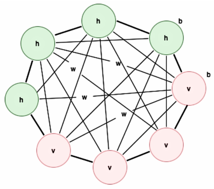
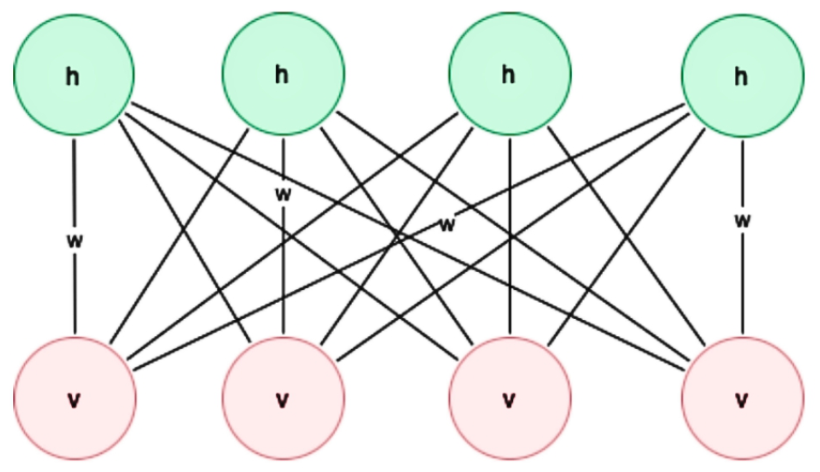
Figure 1 illustrates the architecture of a Boltzmann machine (BM), consisting of visible units v and hidden units h connected through weighted undirected links. The model is parameterized by biases and connection weights. The complete set of model parameters can be represented as follows:
where N denotes the total number of units in the network, represents the bias associated with unit i, and denotes the weight of the connection between units i and j.
Figure 1.
A Boltzmann machine.
Mathematical Formulation
The probabilistic behaviour of a Boltzmann machine is governed by an energy function that assigns an energy value to each configuration of visible and hidden units:
where a and b denote the bias vectors of visible and hidden units, respectively, W represents the interaction matrix between visible and hidden units, and U and V are symmetric matrices describing interactions among visible–visible and hidden–hidden units. A distinguishing characteristic of a BM is that connections are allowed not only between visible and hidden units but also among units within the same layer, resulting in a fully connected architecture.
Based on the energy function, the joint probability distribution over visible and hidden units is defined as follows:
where the denominator corresponds to the partition function:
which ensures that the probability distribution is properly normalized. During training, the model learns weights and biases that assign lower energy to configurations corresponding to the observed data. However, the computation of the partition function remains computationally expensive, motivating the use of approximation methods such as contrastive divergence (CD) for practical learning. In this approach, model parameters are updated using the difference between data-dependent and model-dependent statistics [13].
The Boltzmann machine is described here because it motivates the restricted architecture and because its lateral connections explain the computational cost reported in Section 4.6; it is not evaluated using likelihood in this study.
2.2. Restricted Boltzmann Machines
Restricted Boltzmann machines (RBMs) are a simplified variant of Boltzmann machines designed to improve computational efficiency while preserving the ability to learn complex probability distributions [6]. RBMs belong to the family of energy-based probabilistic graphical models and employ a bipartite architecture consisting of a visible layer and a hidden layer. The visible units represent the observed data, whereas the hidden units capture latent features and dependencies within the data. Owing to their efficient training procedure, RBMs have been widely applied in feature learning, dimensionality reduction, collaborative filtering, and deep learning applications [6].
The primary distinction between a Boltzmann machine and a restricted Boltzmann machine lies in the network connectivity. In a BM, connections are permitted among visible–visible, hidden–hidden, and visible–hidden units, resulting in a fully connected architecture. In contrast, an RBM restricts connections to those between visible and hidden units only, eliminating intra-layer connections. This bipartite structure significantly reduces computational complexity and enables more efficient learning and inference.
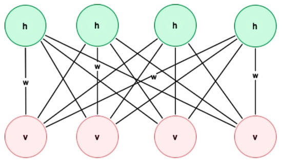
Figure 2 illustrates the architecture of a restricted Boltzmann machine. Let denote the visible units and denote the hidden units, where M and K represent the numbers of visible and hidden units, respectively. Since units within the same layer are not connected, the model exhibits conditional independence properties that simplify probabilistic inference and parameter estimation.
Figure 2.
Simple architecture of an RBM.
The probabilistic behaviour of an RBM is governed by the Gibbs distribution:
where Z is the partition function that normalizes the probability distribution.
The energy function of an RBM is defined as
where a and b represent the bias vectors associated with visible and hidden units, respectively, and W denotes the weight matrix describing interactions between the two layers. Unlike the general Boltzmann machine, the RBM energy function does not contain visible–visible or hidden–hidden interaction terms because such connections are explicitly prohibited by the bipartite architecture.
A key consequence of this structural restriction is conditional independence between units within the same layer. Given the hidden units, the visible units are conditionally independent and can be expressed as
Similarly, given the visible units, the hidden units are conditionally independent:
These conditional independence properties enable efficient Gibbs sampling and make RBMs considerably easier to train than fully connected Boltzmann machines.
Training of RBMs is commonly performed using contrastive divergence (CD), an approximation technique that estimates the gradient of the log-likelihood through a short Gibbs sampling procedure. By alternating between visible and hidden unit updates, CD approximates the model expectations required for parameter learning while avoiding the computational burden associated with exact partition function evaluation. This approach has made RBMs one of the most widely used energy-based models for unsupervised representation learning [6].
2.3. Inference and Partition Function Estimation
Inference is a fundamental component of Boltzmann machines (BMs) and restricted Boltzmann machines (RBMs), enabling the estimation of hidden variables, probabilities, and model expectations required during learning and evaluation [6]. However, exact inference is often computationally difficult due to the large number of possible network configurations.
Another major challenge arises from the partition function, which serves as the normalization constant of the probability distribution and ensures that all probabilities sum to one. In energy-based models such as BMs and RBMs, the computation of the partition function generally requires summation over all possible visible and hidden unit configurations, making exact evaluation computationally intractable for large-scale networks [7].
To address these challenges, several approximate inference and partition function estimation techniques have been developed. Variational inference (VI) provides a tractable framework for approximating complex probability distributions, whereas simple importance sampling (SIS) and annealed importance sampling (AIS) are widely used for estimating partition functions in high-dimensional probabilistic models [7,8]. These methods play an important role in making the training and evaluation of energy-based models computationally feasible.
2.3.1. Simple Importance Sampling (SIS)
Simple importance sampling (SIS) is a Monte Carlo technique used to estimate ratios of partition functions when direct computation is intractable. In the context of energy-based models, SIS provides an efficient approach for approximating normalization constants by drawing samples from a tractable proposal distribution instead of the target distribution [8].
Consider two probability distributions defined on the same sample space :
where and denote unnormalized probability densities. By drawing independent samples from , an unbiased estimate of the ratio of partition functions can be obtained using a Monte Carlo approximation, assuming that whenever :
where and denotes the importance weight associated with sample .
When is chosen such that its partition function can be computed analytically, SIS provides an unbiased estimate of the unknown partition function . However, the effectiveness of the estimator depends strongly on the similarity between and . If the two distributions differ significantly, particularly in high-dimensional spaces, the variance of the estimator may become very large, resulting in poor estimation accuracy [8].
2.3.2. Annealed Importance Sampling (AIS)
Annealed importance sampling (AIS) is an advanced sampling technique widely used for estimating partition functions in energy-based models such as Boltzmann machines (BMs) and restricted Boltzmann machines (RBMs). Since the partition function serves as the normalization constant of the probability distribution, its accurate estimation is essential for evaluating likelihoods and comparing probabilistic models. AIS improves upon simple importance sampling (SIS) by introducing a sequence of intermediate probability distributions that gradually transform an easy-to-sample distribution into the target distribution [8,14].
Let denote an initial distribution with a known partition function and denote the target distribution. AIS constructs a sequence of intermediate distributions
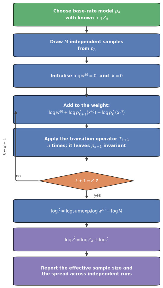
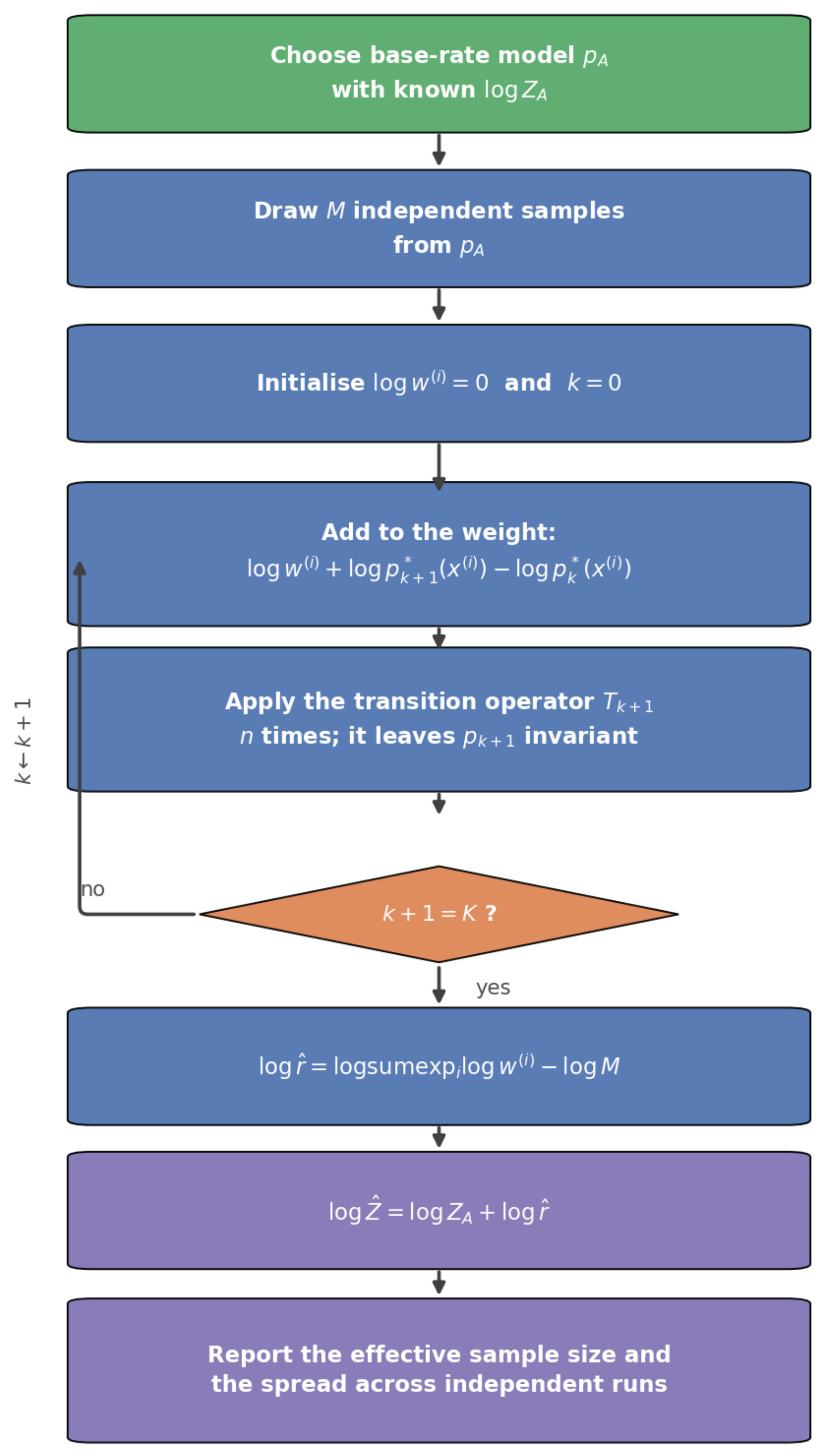
where and . The sequence is traversed forward: an initial sample is drawn from , and successive samples are obtained by transition operators that carry the chain from towards . The weight contributed at step k is the ratio evaluated at a sample , so the denominator is always the earlier distribution of the pair. The conditions are
- whenever , for ; equivalently whenever for . The support of each distribution must contain that of the next one along the path.
- The unnormalized probability density can be evaluated for all intermediate distributions.
- Samples can be generated using a Markov transition operator that leaves invariant.
- Independent samples can be drawn from the initial distribution .
The transition operators satisfy:
A common choice for defining the intermediate distributions is:
where
The parameters define the annealing schedule and control the gradual transition from the initial distribution to the target distribution .
With the sequence of intermediate distributions defined, AIS proceeds by generating samples sequentially through the annealing path. Starting from a sample drawn from the initial distribution , subsequent samples are generated using the corresponding transition operators . The importance weight associated with an AIS run is computed as
where denote samples generated along the sequence of intermediate distributions [7,8]. An important advantage of AIS is that the normalization constants of the intermediate distributions do not need to be computed explicitly. Instead, the accumulated importance weights are used to estimate the ratio of partition functions between the target and initial distributions.
After performing M independent AIS runs, the ratio of partition functions can be estimated as
where denotes the importance weight associated with the AIS run.
The variance of the estimator is given by the following:
where represents the sample variance of the importance weights. Consequently, increasing the number of AIS runs reduces the variance of the estimator and improves estimation accuracy.
The intuition behind AIS is based on decomposing the ratio of partition functions into a sequence of ratios between consecutive intermediate distributions. Consider the identity
If two consecutive intermediate distributions and are sufficiently close, a simple importance sampler can be used to estimate each ratio:
These individual ratios can be combined to approximate the overall partition function ratio:
Since neighbouring distributions are designed to be similar, each ratio can be estimated more accurately than directly estimating the ratio between the initial and target distributions. Consequently, AIS provides more reliable and lower-variance estimates of partition functions than simple importance sampling (SIS). This strategy significantly improves the accuracy of partition function estimation in Boltzmann machines, restricted Boltzmann machines, and other energy-based models [7,8].
Because AIS is unbiased for Z rather than for , Jensen’s inequality gives , so the estimate of the log partition function is low in expectation, and any likelihood computed from it is correspondingly high. The effective sample size of the importance weights,
indicates how far the estimate can be trusted: a collapsed effective sample size means that a handful of chains carry the entire average. The procedure is summarized in Figure 3.
Figure 3.
Annealed importance sampling for the partition function. The loop runs over the K intermediate distributions; at each step, the importance weight is updated, and the chain is moved by a transition operator that leaves the current distribution invariant.
2.3.3. Partition Functions of BMs and RBMs
The partition function plays a fundamental role in Boltzmann machines and restricted Boltzmann machines by serving as the normalization constant of the probability distribution. It ensures that the probabilities assigned to all possible configurations of visible and hidden units sum to one. For a Boltzmann machine, the partition function is defined as
where the summation is taken over all possible configurations of the visible and hidden units. The partition function is essential for computing probabilities, likelihoods, and model expectations.
In practice, it is often more convenient to work with the logarithm of the partition function, known as the log partition function:
The log partition function frequently appears in likelihood-based learning objectives and provides greater numerical stability during optimization and model evaluation.
However, exact computation of the partition function is generally intractable for realistic Boltzmann machines and restricted Boltzmann machines because the number of possible visible–hidden configurations grows exponentially with model size. Consequently, approximation techniques such as annealed importance sampling (AIS) are commonly employed to estimate the partition function and its logarithm [8].
Using AIS, the log partition function can be estimated as
where denotes the log partition function of the base distribution and represents the importance weight obtained from the i-th AIS run. These estimates are widely used for likelihood evaluation, model comparison, and assessing the quality of learned representations in energy-based models.
Computing Partition Functions of Boltzmann Machines
The partition function of a Boltzmann machine can be estimated using annealed importance sampling (AIS) [8]. Following the AIS framework described previously (refer to Equation (15)) and setting , we define the intermediate distributions as
Here, denotes the bias vector of the base-rate model. The first term represents the contribution of the initial distribution and is weighted by . The second term corresponds to the Boltzmann factor of the target model and is scaled by the annealing parameter . As varies from 0 to 1, the influence gradually shifts from the base-rate distribution to the target distribution, thereby defining a smooth sequence of intermediate distributions used in AIS.
These intermediate distributions enable accurate estimation of the partition function while avoiding abrupt transitions between the initial and target distributions.
Computing Partition Functions of Restricted Boltzmann Machines
For restricted Boltzmann machines, AIS employs a tractable base-rate model with parameter vector [15]: zero weight matrix and zero hidden biases, so the hidden units are unconstrained and the visible units are independent Bernoulli variables. Its partition function factorizes as
where M is the number of visible units and K the number of hidden units, so
from which independent samples are generated by drawing each visible unit from . The intermediate distributions are defined as
The annealing parameter is gradually increased from 0 to 1, smoothly transforming the base-rate model into the target RBM. The resulting AIS importance weights are then used to obtain accurate estimates of the RBM partition function [7,8].
2.4. Sum-Product Networks
Sum-product networks (SPNs) are deep probabilistic graphical models introduced by Poon and Domingos to enable tractable inference and efficient representation of complex probability distributions. An SPN is a rooted directed acyclic graph (DAG) composed of sum nodes, product nodes, and leaf nodes. Sum nodes represent probabilistic mixtures, product nodes represent factorized distributions over independent variables, and leaf nodes correspond to distributions over individual variables. In the original formulation, these leaves are indicator variables for the possible values of each variable [9]; later work generalizes them to arbitrary tractable distributions, most often univariate [10,16]. The networks in this study use Bernoulli leaves, one per pixel, which recovers the indicator formulation for binary data.
SPNs provide a hierarchical representation of probability distributions, allowing exact computation of marginal and conditional probabilities in time linear in the size of the network. This property distinguishes SPNs from many traditional probabilistic graphical models, where exact inference is often computationally expensive. Furthermore, SPNs can model high-dimensional distributions while maintaining tractable inference and learning capabilities [9].
The probability distribution represented by a graphical model can generally be expressed as
where denotes a potential function defined over a subset of variables and Z is the partition function given by
By organizing computations through alternating sum and product operations, SPNs provide a compact representation that facilitates efficient probabilistic reasoning and inference.
2.4.1. SPN Architecture
An SPN consists of three types of nodes:
- Leaf Nodes: Represent tractable probability distributions over variables.
- Sum Nodes: Represent weighted mixtures of child distributions.
- Product Nodes: Represent factorized distributions over disjoint variable subsets.
Each edge from a sum node carries a non-negative weight , where denotes the set of children of node i. If the weights of every sum node additionally sum to one,
and the network is complete and decomposable, then its partition function equals one, and each sum node can be interpreted as marginalizing a latent variable whose values index the children [9,17]. The networks used in this study satisfy this by construction, since their sum weights are produced by a softmax.
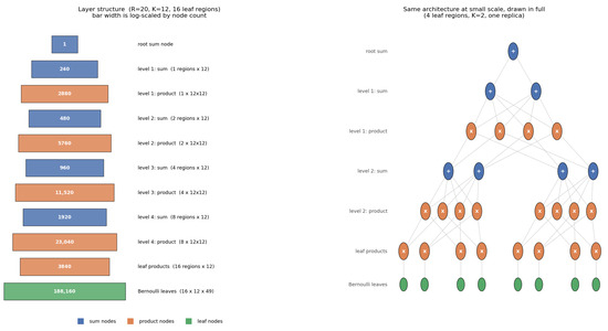
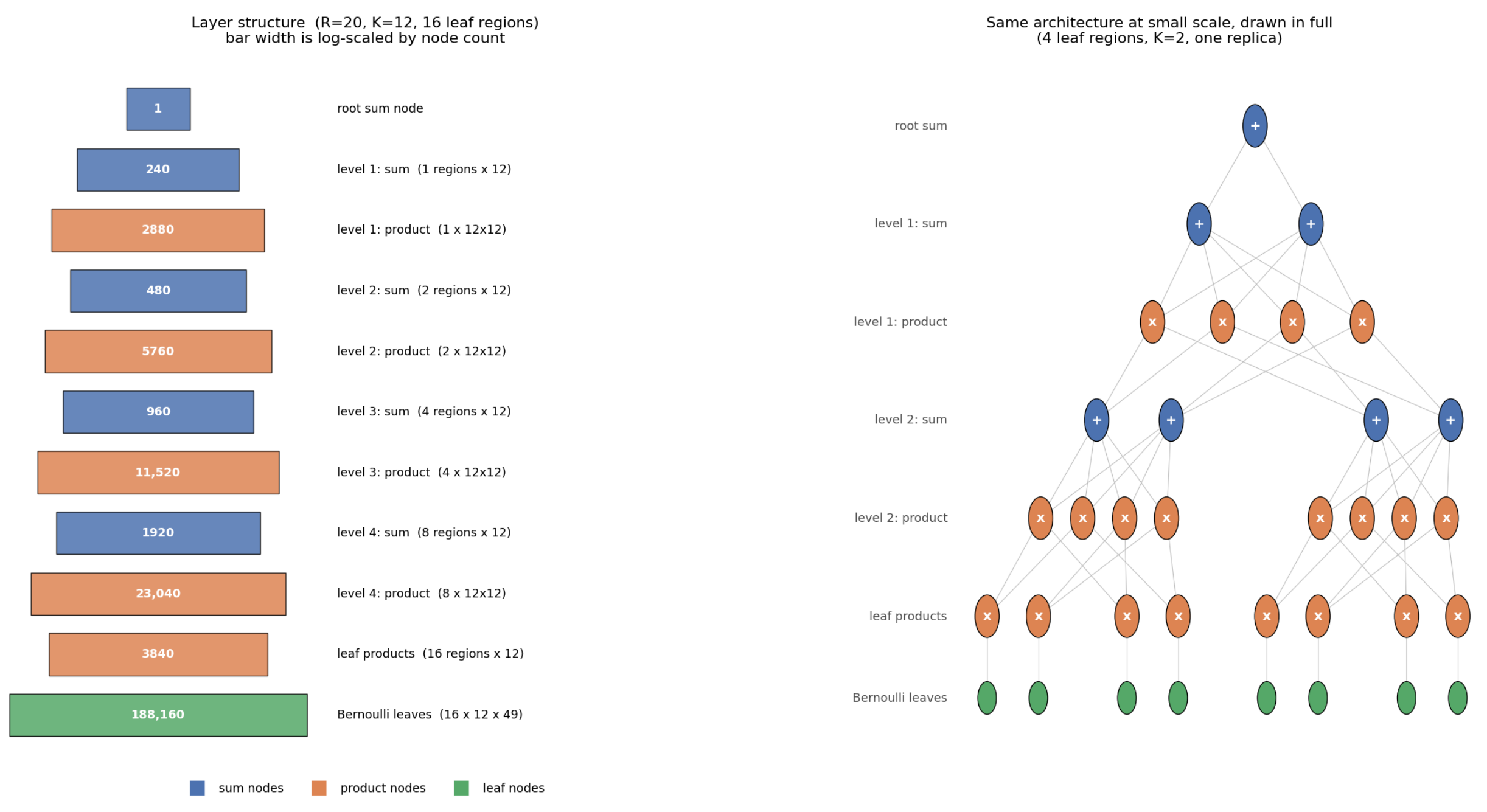
Figure 4 illustrates the hierarchical organization of an SPN, where sum and product nodes are arranged in alternating layers above the leaf distributions. This structure enables efficient computation of probabilistic queries while preserving tractable inference.
Figure 4.
Structure of the network used in this study. (a) Node counts per layer for one replica set of replicas, components and leaf regions; bar width is scaled logarithmically. (b) The same architecture at reduced scale, drawn in full for four leaf regions, and a single replica, showing the alternating sum and product layers between the Bernoulli leaves and the root.
SPNs can be learned from data through parameter learning and structure learning approaches. In particular, structure learning algorithms recursively partition variables and instances to construct valid SPN architectures that satisfy completeness and decomposability constraints. Such approaches have enabled SPNs to be applied effectively to high-dimensional probabilistic modelling tasks [11,12].
The scope of a leaf node corresponds to its associated variable. For an internal node, the scope is defined recursively as the union of the scopes of its children:
The scope of the entire SPN is given by the scope of the root node. Through this hierarchical structure, SPNs efficiently combine local probability distributions into a global representation of the joint distribution [12].
2.4.2. Valid SPNs: Completeness and Decomposability
An SPN is valid if it correctly computes the unnormalized probability of all evidence. Completeness and decomposability together are sufficient for validity: an SPN is complete if all children of a sum node have identical scopes, and decomposable if the children of the same product node have pairwise disjoint scopes [9,10]. Decomposability is strictly stronger than the consistency condition used in the original formulation, which requires only that no variable appear negated in one child of a product node and non-negated in another; decomposability implies consistency [9].
The networks used in this study are complete and decomposable by construction, since each product node combines two regions whose variable sets are disjoint by the partition that defines them. In addition, the weights of every sum node are non-negative and sum to one, so the partition function equals one, and the network output is already a normalized probability computed in a single upward pass.
2.4.3. Probabilistic Inference in SPNs
Inference in SPNs is performed by evaluating the network from the leaf nodes toward the root. Product nodes compute the product of their child values, whereas sum nodes compute weighted combinations of their children. For a sum node i, the output is given by
where denotes the value of child node j, is the corresponding non-negative edge weight, and represents the set of children of node i. The value computed at the root node corresponds to the probability associated with a complete assignment of variables. By incorporating evidence into the leaf indicators, SPNs can efficiently evaluate marginal and conditional probabilities. Owing to their hierarchical structure, marginal and conditional queries can be evaluated exactly in time linear in the size of the network, making them highly tractable probabilistic models [11].
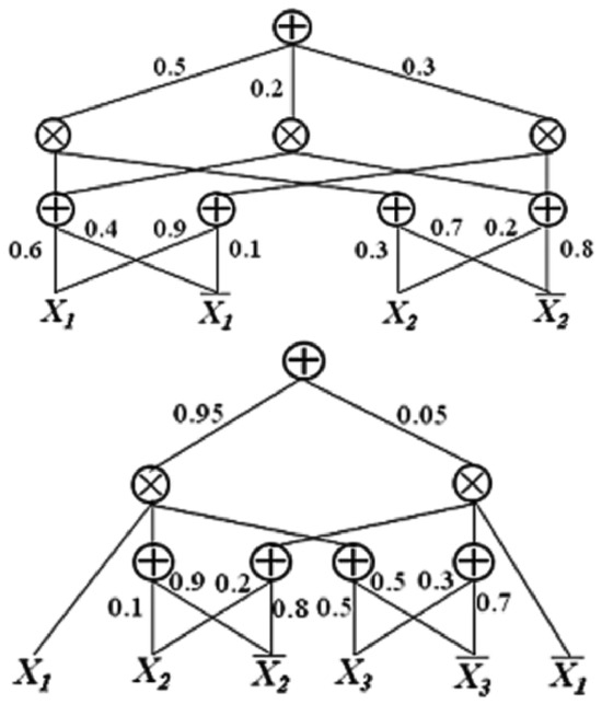
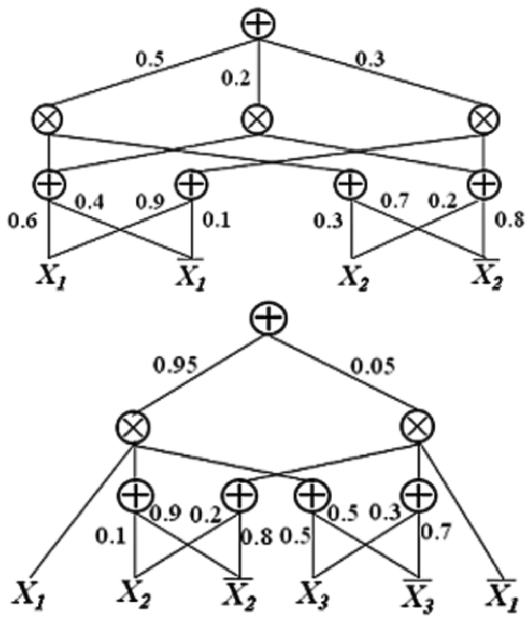
In addition to probabilistic queries, SPNs can be represented as network polynomials composed of weighted sums and products. Figure 5 illustrates an example SPN whose output can be expressed as a polynomial over indicator variables.
Figure 5.
An example sum-product network over two Boolean variables, used to illustrate the network polynomial.
SPNs evaluate complete evidence and marginal queries exactly, in time linear in the size of the network [11]. Most probable explanation queries are handled by replacing the sum at each sum node with a maximum, which maximizes the joint distribution over the variables and the latent sum-node choices; this coincides with the most probable state of the variables alone only when the network is selective, and exact MPE inference in SPNs is NP-hard [17]. Max-product nevertheless remains the standard approach in practice. For the completion experiments in Section 4.4, we therefore use exact conditional marginals thresholded at one-half, which is the optimal predictor for a per-pixel error criterion.
For the SPN shown in Figure 5, the corresponding network polynomial is
This example demonstrates how SPNs compactly represent probability distributions through recursive combinations of sum and product operations, enabling efficient computation of probabilistic queries and exact inference. For example, when a full state is specified as and , the function is represented as . If the evidence e indicates , then becomes . When all indicators are set to 1, the network evaluates to .
2.4.4. Relationship with Bayesian Networks
Bayesian networks (BNs) are probabilistic graphical models represented as directed acyclic graphs (DAGs), where nodes correspond to random variables, and edges encode conditional dependencies among them [18]. The joint probability distribution of a Bayesian network can be factorized as
where denotes the set of parent variables of . This factorization exploits conditional independence relationships to represent complex probability distributions compactly.
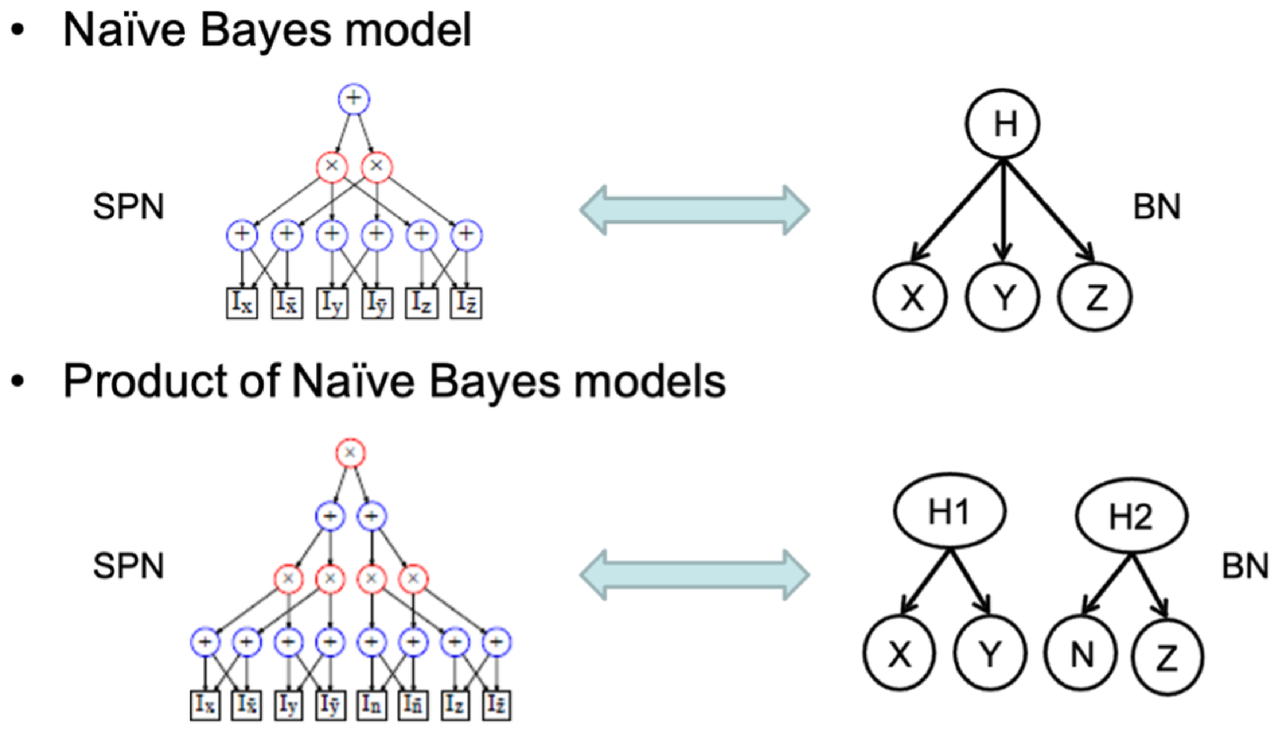
While Bayesian networks represent dependencies through conditional probability relationships, sum-product networks employ hierarchical combinations of sum and product nodes to model probability distributions. The structural properties of completeness and decomposability enable SPNs to perform exact inference efficiently, often with lower computational complexity than traditional Bayesian networks [11,19].
Furthermore, SPNs can be viewed as compact representations of certain Bayesian network structures. Sum nodes correspond to probabilistic mixtures, whereas product nodes capture independencies among subsets of variables. This representation allows SPNs to retain the expressive power of Bayesian networks while providing tractable inference capabilities [16,19].
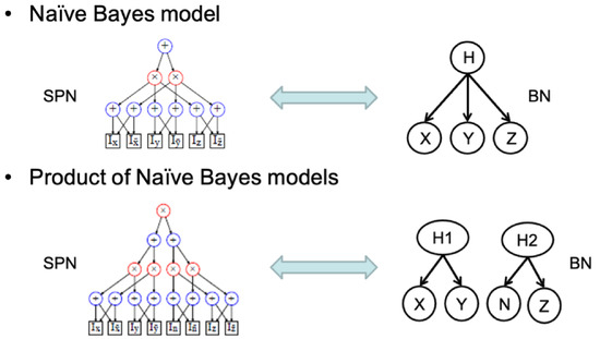
Figure 6 illustrates the correspondence between Bayesian networks and SPN structures. The mapping demonstrates how probabilistic dependencies represented in Bayesian networks can be transformed into hierarchical combinations of sum and product nodes within an SPN. Such a representation facilitates efficient computation of marginal and conditional probabilities while preserving the underlying probabilistic semantics [12,16,19].
Figure 6.
SPNs in relation to Bayesian networks. H, H1, and H2 denote hidden variables, while X, Y, Z, and N denote observed variables.
Overall, SPNs can be regarded as compact and tractable representations of certain Bayesian network structures, combining expressive probabilistic modelling with efficient inference capabilities [11,19].
2.4.5. Network Architecture Used in This Study
The networks evaluated here follow a randomized region graph construction. The pixels are recursively partitioned into a binary tree of depth four, giving leaf regions of variables each. Each region holds sum nodes, and each product node combines one component from each of two child regions, so a region with two children contains product nodes. The construction is repeated over replicas, each using a different partition of the variables, and a single root sum node mixes over all replica–component pairs.
Because every product node combines two regions whose scopes are disjoint by construction, the network is decomposable; because every sum node mixes over products whose scope is exactly that of its own region, it is complete. The sum weights are produced by a softmax,
so they are non-negative and satisfy . The partition function is therefore , and the value at the root is already a normalized probability. Log-likelihoods reported for this model are exact and require no partition function estimation.
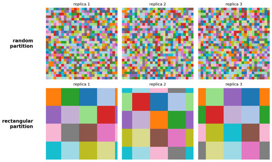
Two region graphs are compared. In the random graph, each replica assigns pixels to leaf regions by an independent uniform permutation of , so a region contains S pixels drawn from anywhere in the image. In the spatial graph, the image is recursively halved into rectangles, so each leaf region is a contiguous patch, and each product node joins two neighbouring patches. Replicas differ in the order in which rows and columns are split and in a cyclic offset applied before splitting, which causes some regions to wrap across the image boundary.
Writing for the number of regions at level ℓ, we find that both configurations contain
giving parameters in total. The two graphs differ only in the assignment of variables to leaf regions, which makes the comparison in Section 4.3 a controlled one.
2.5. Datasets
Experiments were conducted on two widely used benchmark image datasets, Fashion-MNIST and MNIST. Both consist of grayscale images and are commonly employed for evaluating generative and representation learning models. Their relatively simple structure allows efficient training while still providing meaningful benchmarks for comparing model performance, and the contrast between them is useful here: MNIST digits are simple and highly stereotyped, whereas Fashion-MNIST carries greater textural and structural variety.
2.5.1. Fashion-MNIST
Fashion-MNIST consists of 70,000 grayscale images of fashion products distributed across ten categories, including T-shirts, trousers, pullovers, dresses, coats, sandals, shirts, sneakers, bags and ankle boots. Each image has a resolution of pixels, and the dataset is divided into 60,000 training images and 10,000 testing images. It was introduced by Xiao et al. [20] as a drop-in replacement for MNIST and has become a standard benchmark for evaluating machine learning and deep generative models. Compared with handwritten digit datasets, it provides greater visual complexity and is therefore a more challenging benchmark for generative models.
2.5.2. MNIST
MNIST contains 70,000 grayscale images of handwritten digits representing the ten numerical classes from 0 to 9. Each image has a resolution of pixels, with 60,000 images allocated for training and 10,000 reserved for testing. Owing to its simplicity and widespread adoption, MNIST remains one of the most frequently used benchmarks for evaluating machine learning and probabilistic generative models.
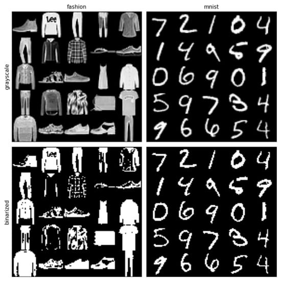
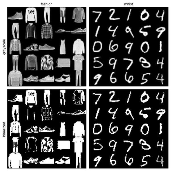
Both datasets are binarized at a fixed threshold of 0.5 before use, since the models compared here are defined over binary variables; the reason is given in Section 3.1. Figure 7 shows test images from both datasets before and after binarization.
Figure 7.
Test images from Fashion-MNIST (left) and MNIST (right), shown as grayscale intensities (top) and after binarization at a threshold of 0.5 (bottom). All experiments use the binarized form.
3. Experimental Setup
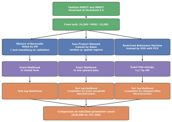
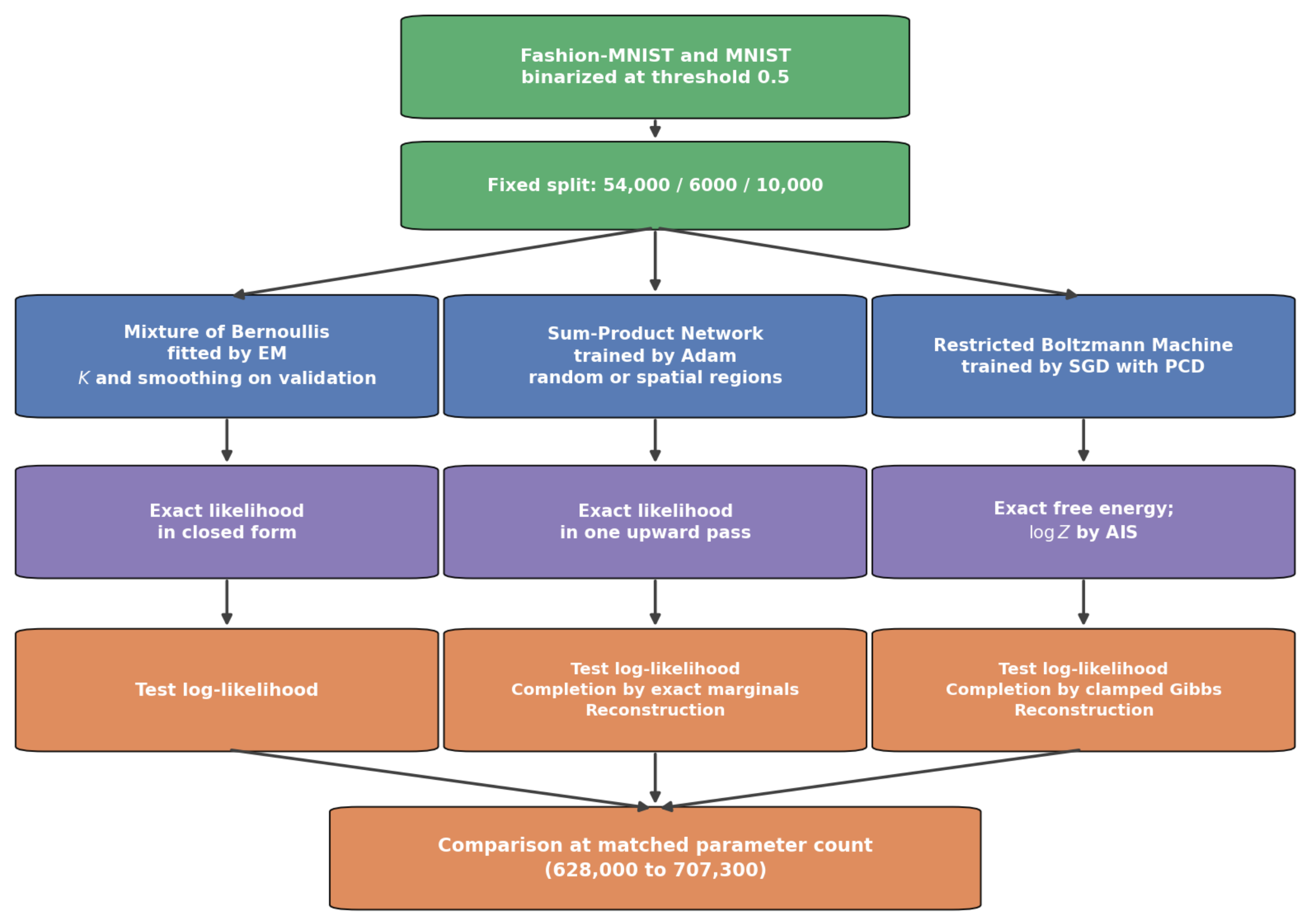
Figure 8 summarises the procedure. All models were trained on the same binarized data under the same split, and compared at a matched parameter count.
Figure 8.
Overview of the experimental procedure. Likelihoods are exact for the mixture baselines and the sum-product network; the restricted Boltzmann machine has an exact per-example free energy but requires annealed importance sampling for its partition function, summarized in Figure 3.
3.1. Data and Splits
Both datasets were binarized at a fixed threshold of 0.5. This is a requirement rather than a preprocessing choice: the energy function of a binary latent variable model and the Bernoulli leaf distributions of a sum-product network are defined over binary variables, and the partition function is not well defined for continuous inputs, so no likelihood can be computed without it. After binarization, 31.5% of Fashion-MNIST pixels and 13.2% of MNIST pixels are active.
The 60,000 training images of each dataset were split into 54,000 for training and 6000 for validation, with the official 10,000 test images held out. The split indices were drawn once from a fixed seed and cached, so every model saw an identical partition. At a batch size of 64 used for the sum-product network and the restricted Boltzmann machine, this gave 844 minibatches per epoch. Test log-likelihood and reconstruction error were computed on all 10,000 test images, as was completion for the sum-product network. Completion for the restricted Boltzmann machine was computed on the first 1000, since each completion required a separate Gibbs sampling run.
3.2. Models and Parameter Matching
Matching the number of hidden units across model families does not match capacity. Lateral connections among 640 hidden units contribute 204,480 parameters that have no counterpart in a restricted architecture, so layer widths were chosen to equalize parameter counts instead. Table 1 lists the configurations.
Table 1.
Model configurations. The final column records how the reported log-likelihood is obtained, which differs by model family and is the principal distinction drawn in this study.
3.3. Training Protocols
Each family was fitted with the standard estimator for that family, so the setup should not be described as having identical training settings across all models. What was held identical was the data, the split, the preprocessing, the evaluation protocol and the parameter budget.
The mixture baselines were fitted by expectation–maximization, which is exact for this model. Parameters were estimated with add- smoothing in the M step, which gives the maximum a posteriori estimate under a symmetric prior. With 800 components, each component receives roughly 67 effective samples, so the smoothing strength materially affects the result; was therefore selected on the validation set alongside K, giving for Fashion-MNIST and for MNIST, with the optimum bracketed on both sides. The validation and test results are summarized in Table 2.
Table 2.
Selection of the smoothing parameter for the mixture baseline with components. Both K and were selected on the validation set. Values in bold are the selected settings.
The choice matters for the conclusions drawn in Section 4.2: at the sum-product network appeared to lead the mixture on MNIST by 4.95 nats, whereas at the selected value the mixture leads by 2.00.
The sum-product network was trained by Adam at a learning rate of 0.001 with a batch size of 64 for 300 epochs, maximizing the exact log-likelihood directly.
The restricted Boltzmann machine was trained by stochastic gradient descent at a learning rate of 0.01 with momentum 0.5 and weight decay , with gradients clipped at a norm of 10. Negative-phase statistics were obtained by persistent contrastive divergence with Gibbs steps per parameter update over 100 persistent chains, burned in for 2000 Gibbs steps before training began. Results are reported at 150 epochs, with 300 epochs included for comparison; the choice is discussed in Section 4.5.
A fixed random seed was used throughout. All experiments ran on a single NVIDIA T4 GPU. One sum-product network epoch took approximately 11.5 s and one restricted Boltzmann machine epoch approximately 4.5 s, giving roughly one hour and twelve minutes, respectively, per training run.
4. Results
4.1. Reconstruction and Completion Examples
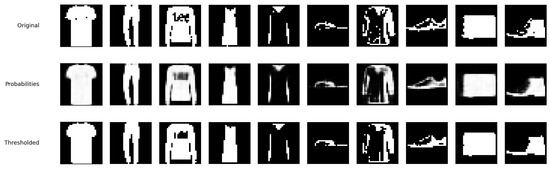
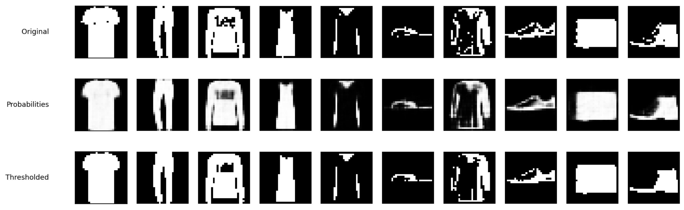
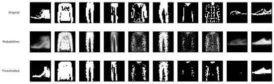
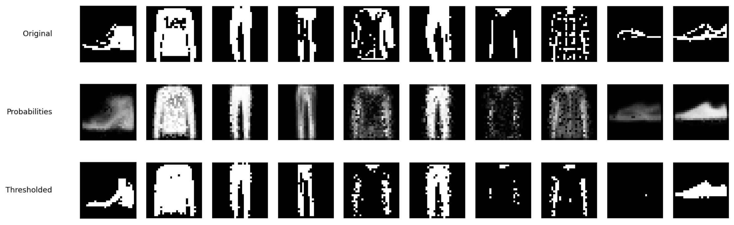
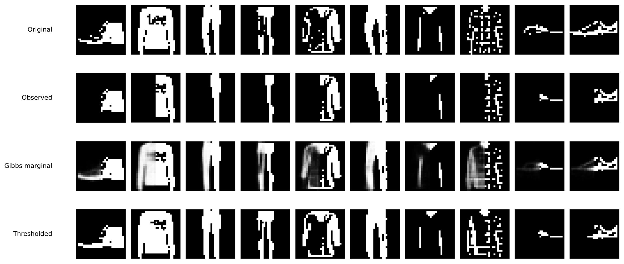
Two tasks are distinguished throughout. In reconstruction, the whole image is presented, and the model regenerates it, so every pixel is observed. In completion, half the image is hidden, and the model must predict the hidden half from the visible half, which is substantially the harder task; the two are not comparable with each other. Figure 9 and Figure 10 show reconstructions on Fashion-MNIST and Figure 11 and Figure 12 show completions with the left half hidden.
Figure 9.
Reconstruction by the restricted Boltzmann machine on Fashion-MNIST. Top: original binarized images. (Middle), labelled “Probabilities”: the conditional marginal of each pixel. (Bottom), labelled “Thresholded”: the same marginals thresholded at one-half. Errors in Table 5 are computed from the thresholded row.
Figure 10.
Reconstruction by the sum-product network on Fashion-MNIST. (Top): original binarized images. (Middle): the conditional marginal of each pixel, computed exactly in a single upward pass. (Bottom): the same marginals thresholded at one-half.
Figure 11.
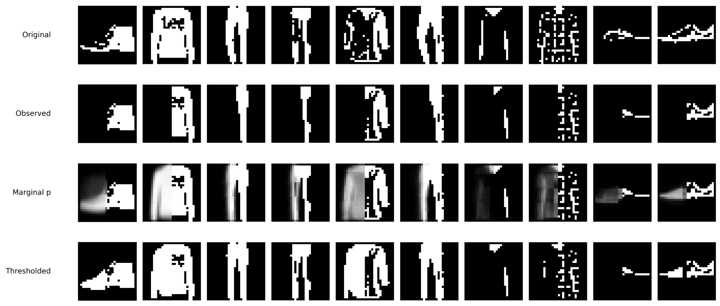
Completion by the restricted Boltzmann machine on Fashion-MNIST with the left half hidden. (Top): original. (Second row): the observed half. (Third row): conditional marginals obtained by clamped Gibbs sampling. (Bottom): marginals thresholded at one-half.
Figure 12.
Completion by the sum-product network on Fashion-MNIST with the left half hidden. (Top): original. (Second row): the observed half. (Third row): the conditional marginal of each hidden pixel, computed exactly. (Bottom): the same marginals thresholded at one-half. Unlike Figure 11, where the marginals are estimated by Gibbs sampling, these are exact.
Both models preserve the class-specific structure of the inputs under reconstruction. Upon completion, the visible half constrains the prediction, and both produce garments consistent with the observed side rather than generic shapes; where the two halves of a garment differ, the models fill in a plausible continuation rather than reproducing the visible half. The corresponding MNIST figures are given in Appendix A.
4.2. Test Log-Likelihood
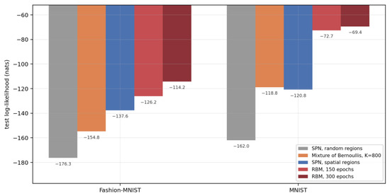
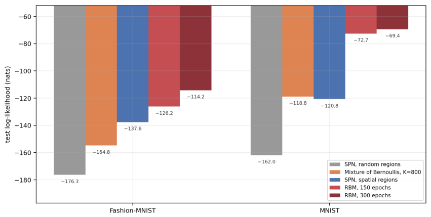
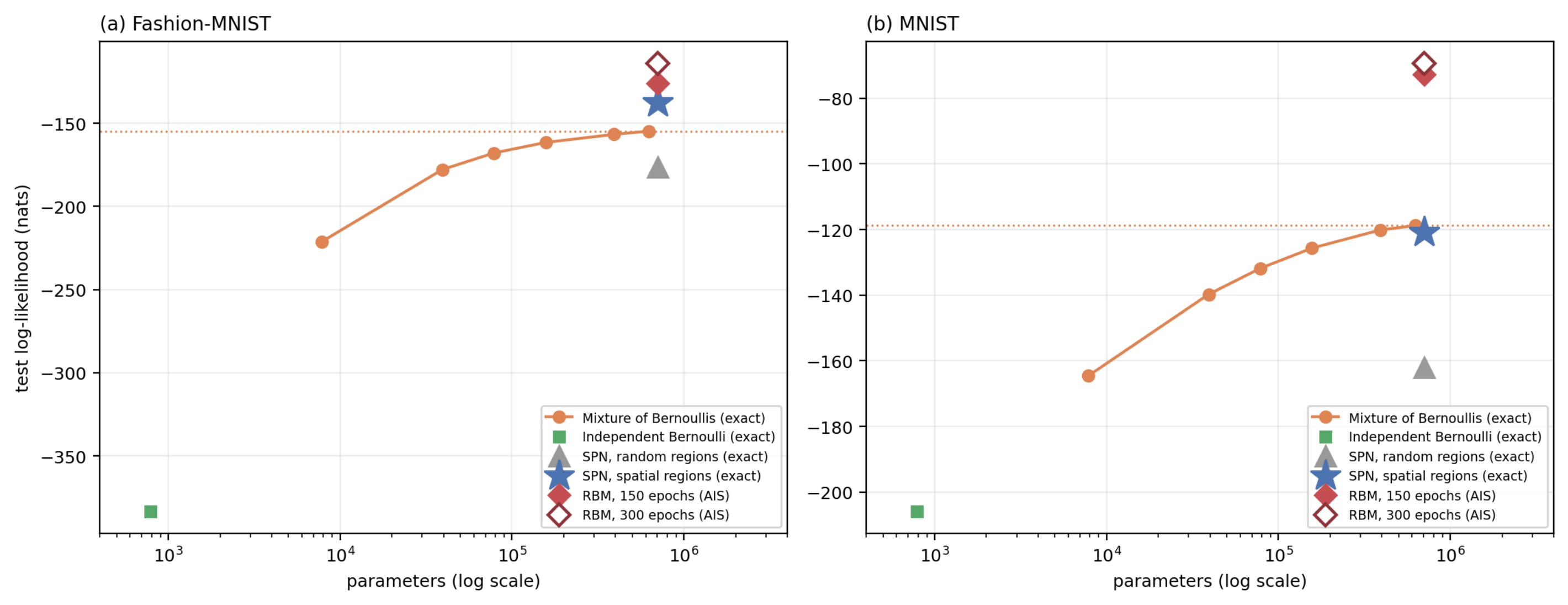
Table 3 reports the mean test log-likelihood of every model on both datasets, and Figure 13 shows the models whose parameter counts are comparable. Standard errors over the 10,000 test images range from 0.20 to 0.91 nats, so every difference discussed below is far outside sampling noise. All values are exact except those for the Restricted Boltzmann Machine, which require annealed importance sampling.
Table 3.
Mean test log-likelihood in nats, with standard errors over the 10,000 test images. Larger is better. The mixture is reported at its validation-selected smoothing, for Fashion-MNIST and for MNIST.
Figure 13.
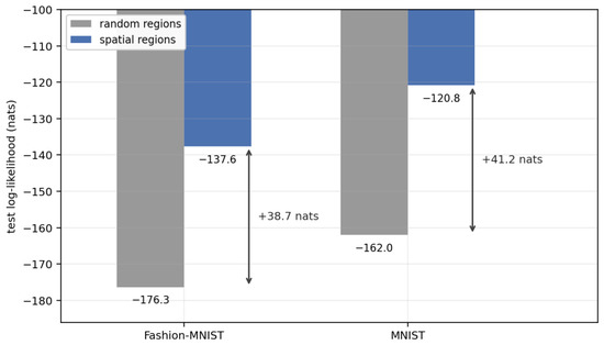
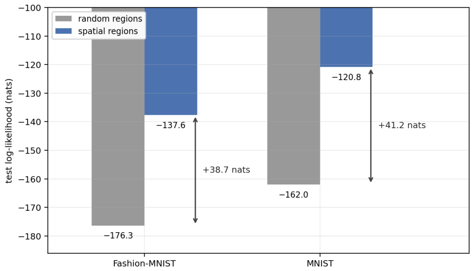
Test log-likelihood of the models with comparable parameter counts, between 628,000 and 707,300. The two sum-product networks differ only in how pixels are assigned to leaf regions; the comparison is examined in Section 4.3.
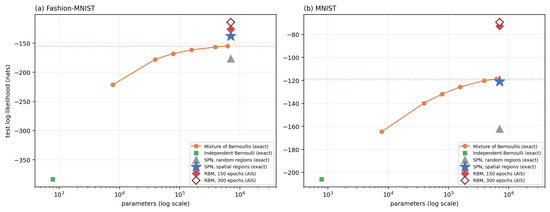
The mixture improves steadily with capacity but with clear diminishing returns. Multiplying its parameters eightfold, from 78,500 at to 628,000 at , buys 13.1 nats on Fashion-MNIST and 13.0 on MNIST, and the final step from to , a 1.6-fold increase in parameters, contributes only 2.0 and 1.3 nats, respectively. Figure 14 places every model on the same axis.
Figure 14.
Test log-likelihood against parameter count for (a) Fashion-MNIST and (b) MNIST. The dotted line marks the best flat mixture. Legend entries indicate whether each value is exact or an AIS estimate.
At comparable capacity, the sum-product network with a spatial region graph exceeds the flat mixture by 17.2 nats on Fashion-MNIST but falls 2.0 nats short of it on MNIST. The restricted Boltzmann machine leads every tractable model on both datasets: on Fashion-MNIST it exceeds the sum-product network, the best tractable model there, by 11.4 nats; on MNIST it exceeds the flat mixture, the best tractable model there, by 46.1 nats.
4.3. The Region Graph
The two sum-product networks differ in one respect only: which pixels are assigned to which leaf region. Parameter count, sum, product and leaf node counts, depth, optimizer, learning rate, batch size, number of epochs and random seed are all identical. Figure 15 shows the two assignments and Figure 16 the resulting difference.
Figure 15.
Assignment of pixels to leaf regions for three replicas. Each colour marks one of the 16 leaf regions. Top row: the random region graph, where each region draws its 49 pixels from anywhere in the image. Bottom row: the spatial region graph, where each region is a contiguous patch; replicas differ in the order of row and column splits and in a cyclic offset, which causes some regions to wrap across the image boundary.
Figure 16.
Test log-likelihood under the two region graphs shown in Figure 15. Both networks have 706,800 parameters and identical numbers of sum, product and leaf nodes; they differ only in which pixels are assigned to which leaf region.
Changing the region graph alone is worth 38.7 nats on Fashion-MNIST and 41.2 on MNIST, the largest single effect measured anywhere in this study and three times what an eightfold increase in mixture capacity achieves. The third row of Table 4 is the more striking one: with a random region graph, the network is worse than a flat mixture of comparable size on both datasets, by 21.5 and 43.2 nats.
Table 4.
The ablation stated as differences in test log-likelihood, in nats. A positive value favours the first model named.
4.4. Completion and Reconstruction
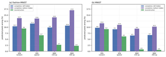
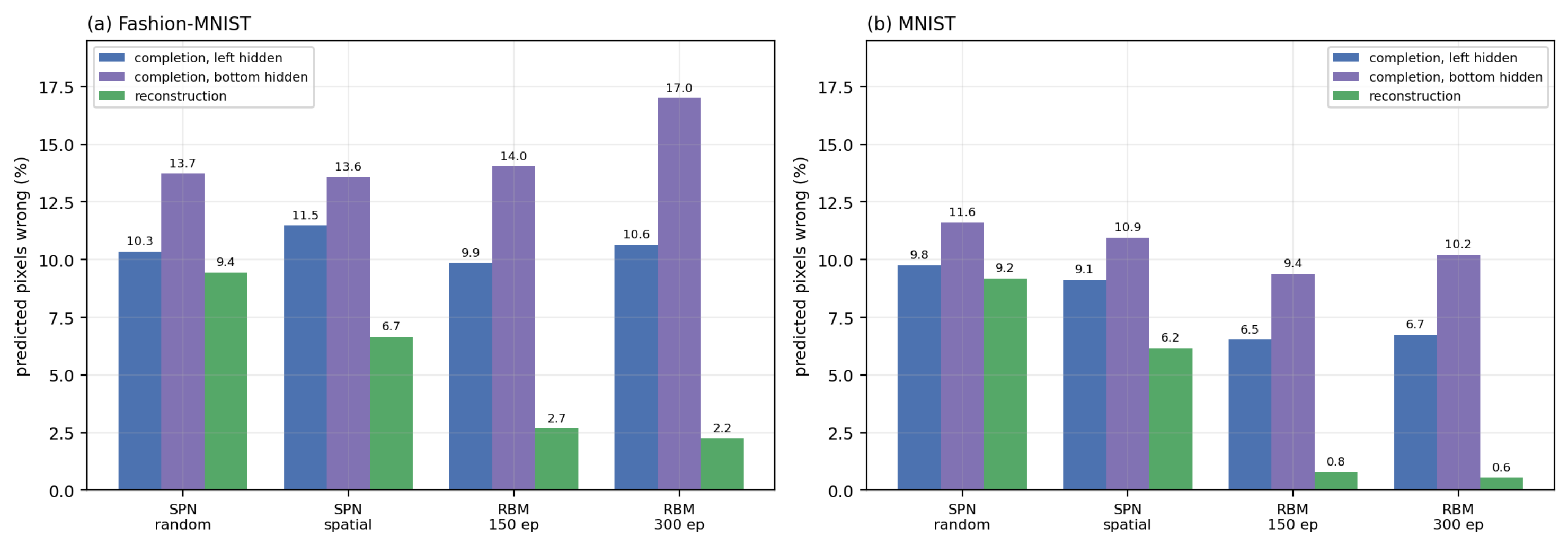
Table 5 reports the percentage of predicted pixels that are wrong, which on binary data equals the mean squared error on the zero-to-one scale. Figure 17 summarizes these pixel-error results for Fashion-MNIST and MNIST.
Table 5.
Pixel error as a percentage of predicted pixels. Completion hides half the image and predicts it; reconstruction observes every pixel. The two are not comparable with each other. Completion for the sum-product network and all reconstruction figures are computed on the full 10,000 test images; completion for the restricted Boltzmann machine is computed on the first 1000, since each completion requires a separate Gibbs sampling run.
Figure 17.
Pixel error for (a) Fashion-MNIST and (b) MNIST.
Three qualifications apply to this table. First, reconstruction observes every pixel while completion hides half the image, so the reconstruction column is not comparable with the completion columns. With more hidden units than visible ones, reconstruction approaches an identity mapping and says correspondingly little about the learned density.
Second, completion error depends on the region graph in a way that log-likelihood does not. Under a left-half mask, 92 of the 320 leaf regions in the spatial network receive no observed pixel at all and must be inferred entirely through the hierarchy, against none under a random partition, where every region contains pixels from both halves of the image. This is why the random network scores better on Fashion-MNIST completion despite a likelihood 38.7 nats worse: the two networks are not solving equally hard versions of the task. Log-likelihood carries no such dependence and is the metric to lead with.
Third, the sum-product network’s completions use exact conditional marginals thresholded at one-half rather than max-product. For a per-pixel criterion, the conditional marginal is the optimal predictor, and it improves on max-product in every configuration tested, by 2.81 and 1.50 percentage points on Fashion-MNIST and by 0.64 and 1.71 on MNIST for the left and bottom masks. Because the network computes those marginals exactly in a single pass, it can use the predictor the metric calls for; where marginals are available only through sampling, that choice is not cleanly available. These results are summarized in Table 6.
Table 6.
Completion error of the sum-product network with the spatial region graph under two predictors, as a percentage of predicted pixels. The conditional marginal is the optimal predictor for a per-pixel criterion; the network computes it exactly in a single upward pass.
4.5. Partition Function Estimation
The per-example free energy of the restricted Boltzmann machine is exact, but requires annealed importance sampling, which is biased low in expectation and therefore biases the likelihood high. Table 7 records the estimate under several annealing budgets.
Table 7.
Estimates of for the restricted Boltzmann machine under varying annealing budgets, with the effective sample size of the importance weights and the standard deviation across three independent runs.
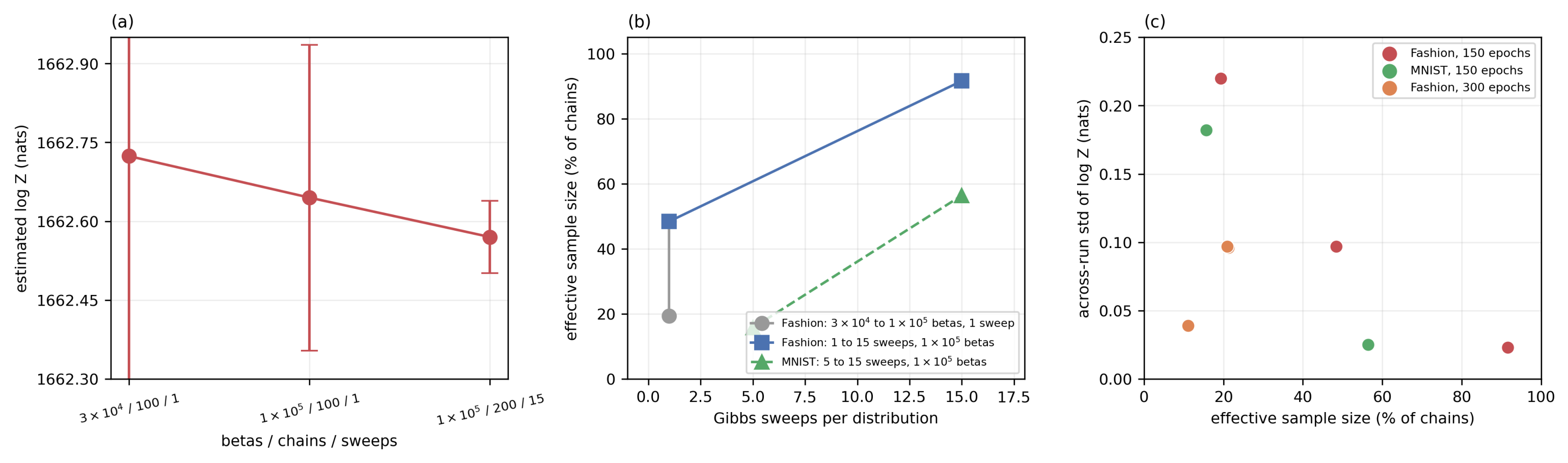
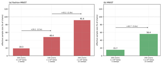
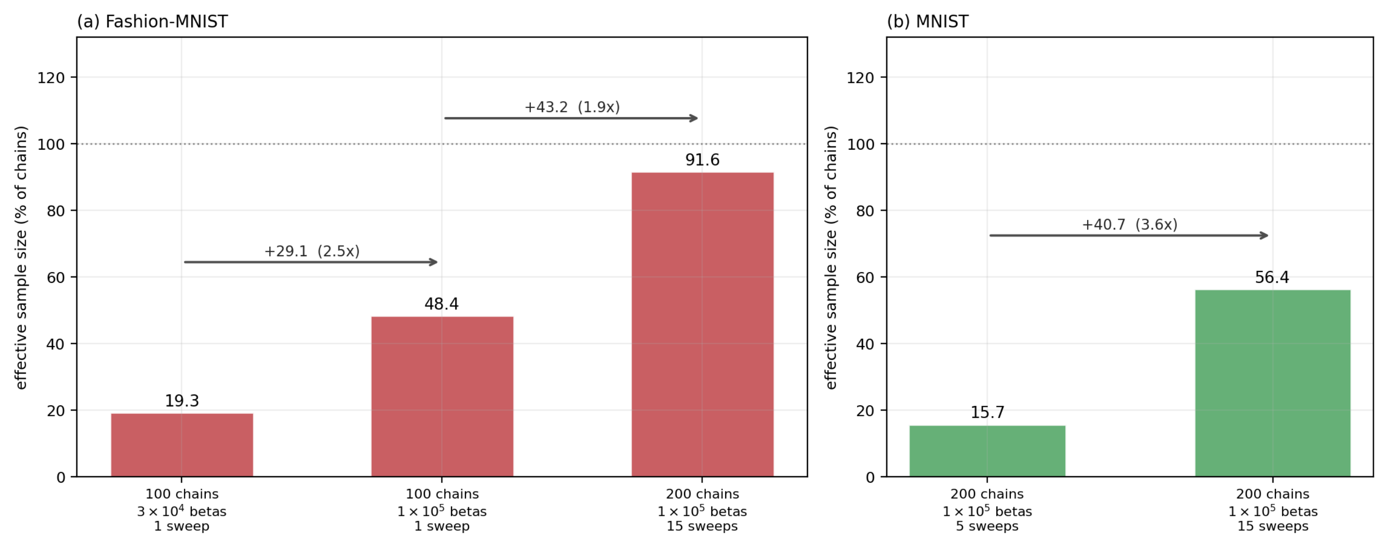
The estimate is insensitive to the budget. At 150 epochs on Fashion-MNIST, across a 3.3-fold change in the annealing schedule and a 15-fold change in the number of Gibbs sweeps, varies by 0.154 nats. On MNIST, where the schedule and the number of chains were held fixed, and only the sweeps were varied from 5 to 15, it varies by 0.006 nats. At 300 epochs on Fashion-MNIST, where the effective sample size is lowest, tripling either the schedule or the number of sweeps moves the estimate by at most 0.102 nats. Had the estimate been materially biased, improving the mixing would have moved it. Figure 18 summarizes the effective sample sizes across these configurations.
Figure 18.
Effective sample size of the importance weights at 150 epochs for (a) Fashion-MNIST and (b) MNIST, as a percentage of the chains used. The dotted line marks 100%, where all weights are equal. On MNIST, the chains and schedule are held fixed, and only the sweeps vary; on Fashion-MNIST, the schedule is lengthened first, then both the sweeps and the number of chains are raised, so the final step confounds the two.
Additional Gibbs sweeps raise the effective sample size far more than a longer schedule does: on MNIST, holding chains and schedule fixed, raising the sweeps from 5 to 15 increases it 3.6-fold. This is expected of a multimodal target, since extra steps shorten the distance between consecutive distributions, whereas extra sweeps allow each chain to equilibrate at the distribution it is currently on.
The implementation was validated against exact enumeration on models small enough to enumerate, where it recovers to within 0.005 nats with effective sample sizes above 296 of 300 across three choices of base-rate distribution. The reduced effective sample size on the trained models therefore reflects the difficulty of the target rather than the estimator.
The two kinds of variation in Table 7 test different things: agreement between estimates at different budgets tests for bias, since the bias of the estimator is a function of the budget, whereas agreement between runs at the same budget tests only variance.
Two further checks support the estimate. The base-rate model provides an analytic lower bound on , and the estimate exceeds it by 13.6 nats on Fashion-MNIST at 150 epochs, so it has not collapsed towards the initial distribution. No test image received a positive log-probability, which would indicate an underestimated partition function.
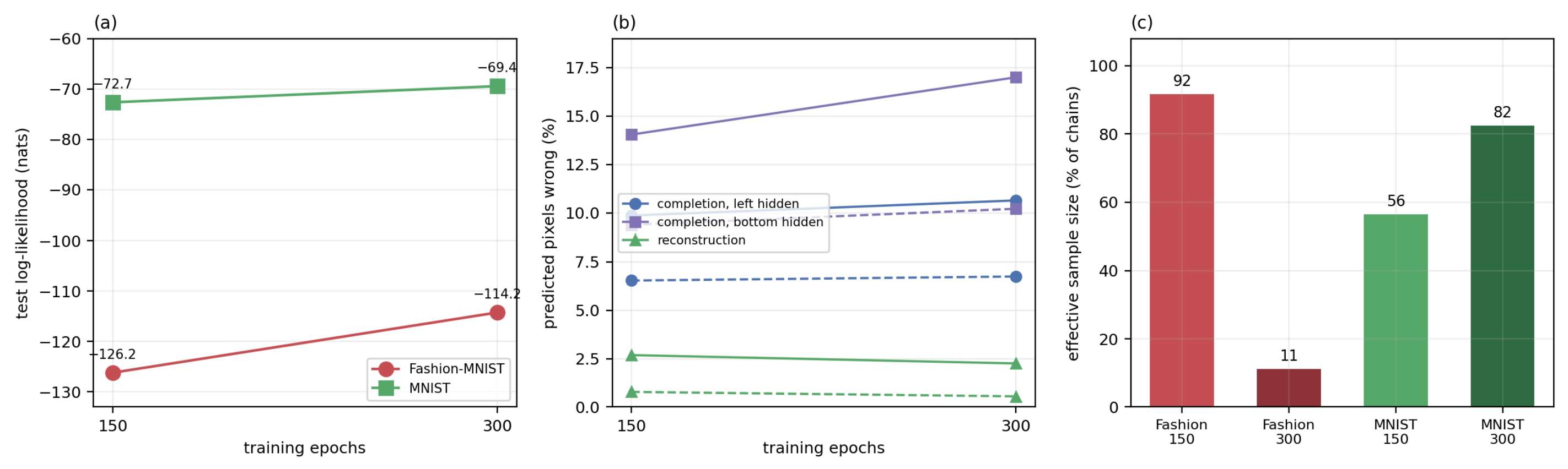
Figure 19 compares the two training lengths. Longer training improves the likelihood and reconstruction on both datasets while completion degrades, illustrating why reconstruction error is a poor proxy for generative quality. At a fixed budget of 100,000 intermediate distributions, 200 chains and 15 sweeps, the effective sample size falls from 92% to 11% on Fashion-MNIST while rising from 56% to 82% on MNIST. Results at 150 epochs are reported as primary because the estimator is best behaved there. This is the conservative choice: the 150-epoch model has the lower reported likelihood of the two, so the comparisons in Section 4.2 understate rather than overstate the performance of the restricted Boltzmann machine.
Figure 19.
Effect of training length on the restricted Boltzmann machine. (a) Test log-likelihood. (b) Pixel error; solid lines—Fashion-MNIST; dashed—MNIST. (c) Effective sample size of the AIS weights.
4.6. The Boltzmann Machine
Lateral connections among the hidden units remove their conditional independence, so the layer can no longer be updated in parallel. Each negative-phase step requires 640 sequential single-site Gibbs updates compared with two parallel matrix products for the restricted Boltzmann machine. At the latter’s settings, a single epoch exceeded ten minutes on the hardware used here, compared with 4.5 s. Raising the batch size to 256 and resampling 64 randomly selected units per sweep, which leaves the model distribution invariant and changes only the mixing rate, reduced this to roughly 37 s per epoch.
Even at that rate, the model had not converged after 50 epochs: the free energy was still rising, and the weight norm had reached 40% of the converged restricted Boltzmann machine’s. Reconstruction and completion errors from an unconverged model would not be comparable across architectures and are therefore not reported.
The learned weights are nonetheless informative. Table 8 gives the Frobenius norms of the two weight matrices.
Table 8.
Learned weight norms and runtime for the Boltzmann machine after 50 epochs. W denotes the cross-layer weight matrix and the lateral matrix among hidden units.
The lateral connections reach roughly one-half to six-tenths of the Frobenius norm of the cross-layer matrix on both datasets. The additional connectivity is therefore used rather than being vestigial, but the cross-layer structure, which the restricted Boltzmann machine also possesses, carries approximately twice the weight. This suggests that the two architectures would not differ greatly on these datasets, although the present experiments do not test that directly.
5. Discussion
5.1. Interpretation of the Findings
Three results follow from the comparisons above.
A misaligned hierarchy is worse than no hierarchy. With leaf regions assigned at random, the sum-product network loses to a flat mixture of comparable size on both datasets, by 21.5 nats on Fashion-MNIST and 43.2 on MNIST. The product nodes in such a network assert independence between sets of pixels that have no spatial relationship, so the hierarchy has no structure to exploit and spends its capacity encoding arbitrary groupings. Depth built over the wrong partition of the variables does not merely fail to help; it costs, relative to a model with no hierarchy at all. This is the more consequential half of the region graph result, and it does not appear to be widely appreciated.
Given alignment, the benefit depends on the data. Once the regions follow the spatial layout of the image, the same network exceeds the flat mixture by 17.2 nats on Fashion-MNIST but falls 2.0 nats short on MNIST. MNIST digits are simple, stereotyped and heavily shared across the dataset, so 800 whole-image prototypes already cover the space; Fashion-MNIST carries more textural and structural variety, and there, depth pays for itself several times over. The value of hierarchical structure is thus a property of the interaction between model and data rather than of the model alone.
Tractable inference is bought at a cost in modelling power. The restricted Boltzmann machine leads every tractable model tested at a matched parameter count. On Fashion-MNIST it exceeds the sum-product network, the best tractable model there, by 11.4 nats; on MNIST it exceeds the flat mixture, the best tractable model there, by 46.1. The sum-product network returns an exact likelihood and exact marginals from a single upward pass, while the restricted Boltzmann machine’s likelihood is available only through annealed importance sampling with the diagnostics of Section 4.5. The gap between them is the price of that guarantee, and on these datasets it is substantial.
The practical consequence of tractability is visible in the completion results. For a per-pixel criterion, the optimal prediction is the conditional marginal, and the sum-product network can compute it exactly, improving on max-product in every configuration tested. Where marginals are available only by sampling, that choice is not cleanly available. Exact inference does not make a model a better density estimator, but it does let the model answer the question a given metric actually asks.
5.2. Sum-Product Networks: Opportunities and Challenges
The results above suggest that the practical question for sum-product networks is not whether tractable inference is desirable, which it plainly is, but whether a region graph suited to the data can be found. On image data, the appropriate structure is evident, and the gain from using it is large. On domains without an obvious notion of locality, it is not, and the random-region results indicate what is lost when the structure is misaligned: a network that underperforms a model with no hierarchy at all despite carrying the same number of parameters.
Structure learning therefore remains the central open problem, and these results sharpen why. It is usually framed as searching a large space of valid structures efficiently [11,12]; the question here is instead how to find one whose independence assumptions match the data, since the difference between a matched and a mismatched structure at fixed capacity is far larger than the difference between a small and a large model.
6. Limitations and Future Work
Several limitations should be stated explicitly.
Binarization. All models are trained on data binarized at a fixed threshold of 0.5, which is required for the partition function to be well defined but discards information. Absolute likelihoods are therefore not comparable with published values obtained under stochastic binarization, which is the more common convention in this literature [15], and no cross-paper numerical comparison is claimed. The comparisons within this study are valid because every model sees identical data.
The Boltzmann machine is not evaluated using likelihood. Its per-example term has no closed form, because lateral connections remove the conditional independence of the hidden units that the restricted architecture relies on. A likelihood estimate would therefore require a variational lower bound on that sum in addition to an annealed importance sampling estimate of , with annealing carried out in the joint space using sequential sweeps [5]. Combined with the training cost reported in Section 4.6, this placed a comparable evaluation beyond the compute available. What is reported for this model is confined to quantities that a partially trained network can support.
Approximate likelihoods. Values reported for the restricted Boltzmann machine are estimates rather than exact quantities and are biased upward, since annealed importance sampling underestimates in expectation [8]. The diagnostics in Section 4.5 bound how far this matters, but they do not eliminate it. Values for the sum-product network and the mixture baselines carry no such caveat.
Completion error and the region graph. As noted in Section 4.4, completion error depends on how many leaf regions receive evidence under a given mask, so completion figures should not be compared across networks with different region graphs.
A single seed. Every result comes from one random seed. The larger differences reported here run to tens of nats and no seed would reverse them, but the 2.0-nat gap between the sum-product network and the flat mixture on MNIST is small enough that repeating that comparison across seeds would be worthwhile before treating it as settled.
Future work follows directly. Evaluating the Boltzmann machine on the same footing as the other models requires either more compute or a cheaper estimator for its per-example term. Extending the comparison to data without an obvious spatial structure would test whether the region graph result generalizes beyond images. Learning the region graph from data, rather than choosing between a random and a rectangular one, is the natural next step given how much the choice matters.
7. Conclusions
This study compared sum-product networks, mixtures of Bernoullis and a restricted Boltzmann machine on binarized Fashion-MNIST and MNIST under identical preprocessing, identical data splits and matched parameter counts, evaluating every model by test log-likelihood on a common scale.
Three findings emerged. First, the structure of the region graph matters more than the size of the network: changing which pixels are grouped into which leaf region, at a fixed parameter count, is worth 38.7 nats on Fashion-MNIST and 41.2 nats on MNIST, whereas multiplying the capacity of a flat mixture eightfold buys about 13 nats. A network whose regions are misaligned with the data is worse than a model with no hierarchy at all. Second, once the regions are aligned, the benefit of hierarchy depends on the data: 17.2 nats on Fashion-MNIST and nats on MNIST, where a flat mixture is the better model. Third, the restricted Boltzmann machine outperforms every tractable model tested at matched capacity, leading the best of them by 11.4 nats on Fashion-MNIST and 46.1 nats on MNIST, which quantifies the cost of guaranteeing exact inference.
The evaluation also illustrates what tractability buys in practice. Sum-product network likelihoods are exact and require no estimation, whereas those of the restricted Boltzmann machine rest on annealed importance sampling and must be reported with the effective sample size and the sensitivity of the estimate to the annealing budget. For completion, exact marginals allow the network to use the predictor the metric calls for and improve on max-product in every configuration tested.
The Boltzmann machine was not evaluated using likelihood. Lateral connections prevent parallel layer updates and make both training and partition function estimation substantially more expensive than for the restricted architecture, placing a comparable evaluation beyond the compute available. Its learned lateral weights reach roughly half the Frobenius norm of the cross-layer matrix, indicating that the additional connectivity is used but that the cross-layer weights, which the restricted architecture also has, carry roughly twice as much.
Author Contributions
Conceptualization, M.A.A. and S.E.A.; methodology, M.A.A. and S.E.A.; software, M.A.A.; validation, M.A.A. and S.E.A.; formal analysis, M.A.A.; investigation, M.A.A.; data curation, M.A.A.; writing—original draft preparation, M.A.A.; writing—review and editing, M.A.A. and S.E.A.; visualization, M.A.A.; supervision, S.E.A.; funding acquisition, S.E.A. All authors have read and agreed to the published version of the manuscript.
Funding
This research was supported by the Natural Sciences and Engineering Research Council of Canada (NSERC) Discovery Grant RGPIN-2023-03693.
Data Availability Statement
The datasets used in this study are publicly available. Fashion-MNIST is available at https://github.com/zalandoresearch/fashion-mnist (accessed on 10 August 2026) and MNIST is available at http://yann.lecun.com/exdb/mnist/ (accessed on 10 August 2026). The implementation details supporting the findings of this study are available from the corresponding author upon reasonable request.
Conflicts of Interest
The authors declare no conflicts of interest.
Abbreviations
The following abbreviations are used in this manuscript:
| AIS | Annealed Importance Sampling |
| BM | Boltzmann Machine |
| EBM | Energy-Based Model |
| ESS | Effective Sample Size |
| MPE | Most Probable Explanation |
| RBM | Restricted Boltzmann Machine |
| CD | Contrastive Divergence |
| SIS | Simple Importance Sampling |
| SPN | Sum-Product Network |
Appendix A. Additional Figures
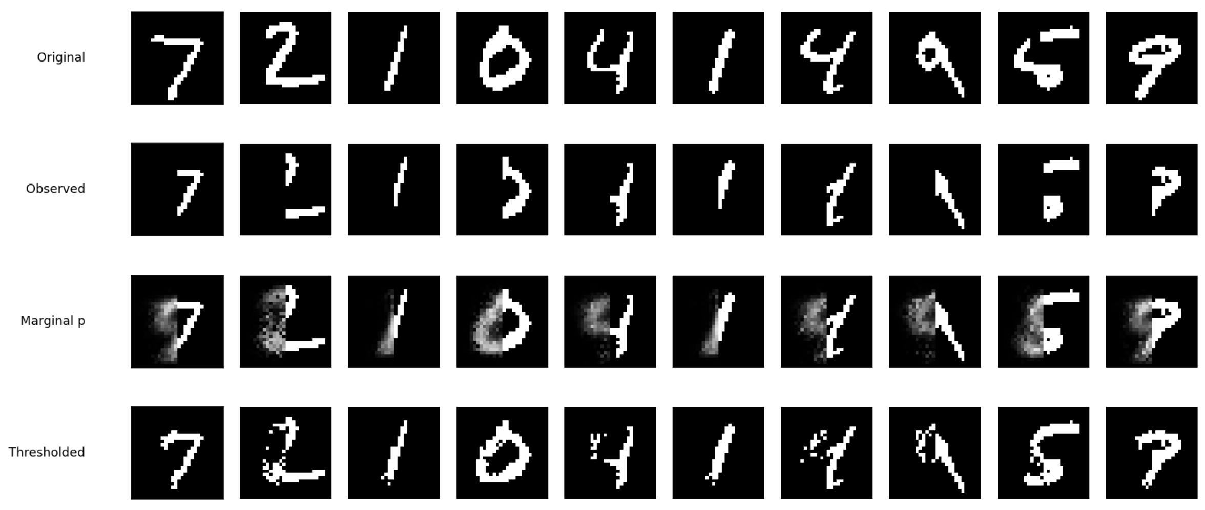
This appendix provides additional qualitative results for MNIST together with the convergence analysis of the annealed importance sampling (AIS) estimator. The figure layouts and notation follow the corresponding figures presented in Section 4.
Appendix A.1. MNIST
Figure A1.
Reconstruction by the restricted Boltzmann machine on MNIST. (Top): original binarized images. (Middle): conditional marginals. (Bottom): the same marginals thresholded at one-half.
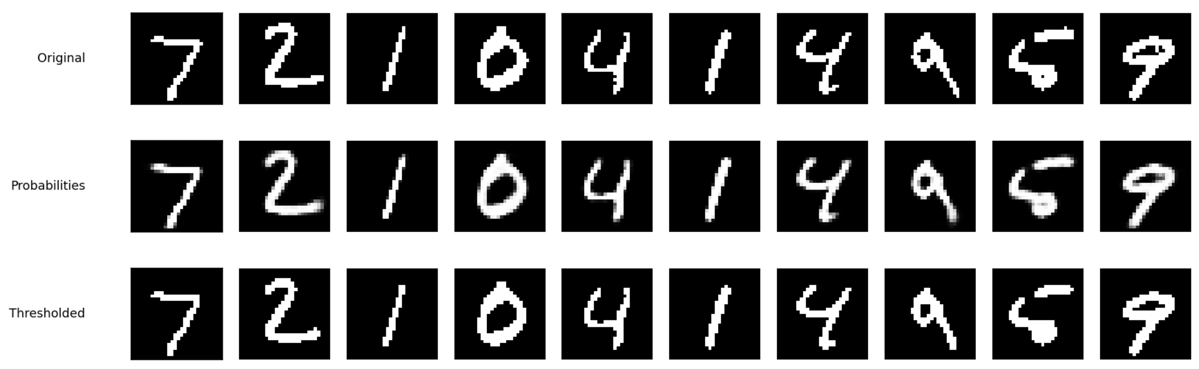
Figure A2.
Reconstruction by the sum-product network on MNIST. (Top): original binarized images. (Middle): conditional marginals, computed exactly. (Bottom): the same marginals thresholded at one-half.
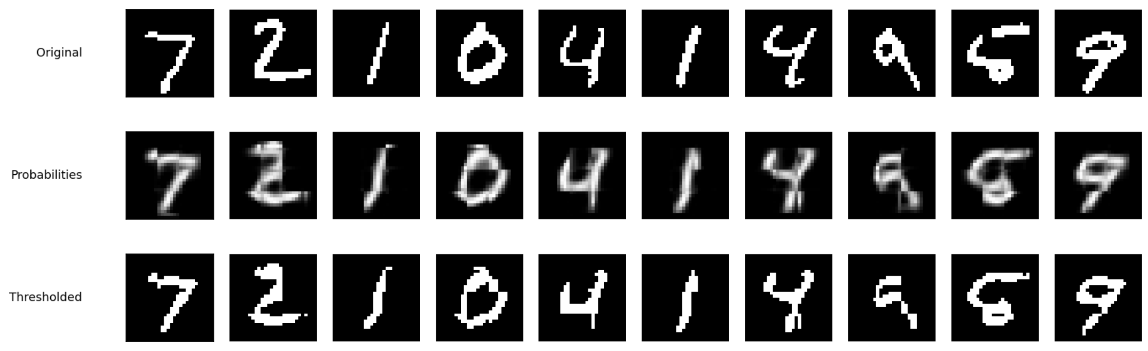
Figure A3.
Completion by the restricted Boltzmann machine on MNIST with the left half hidden. (Top): original. (Second row): the observed half. (Third row): conditional marginals estimated by clamped Gibbs sampling. (Bottom): marginals thresholded at one-half.
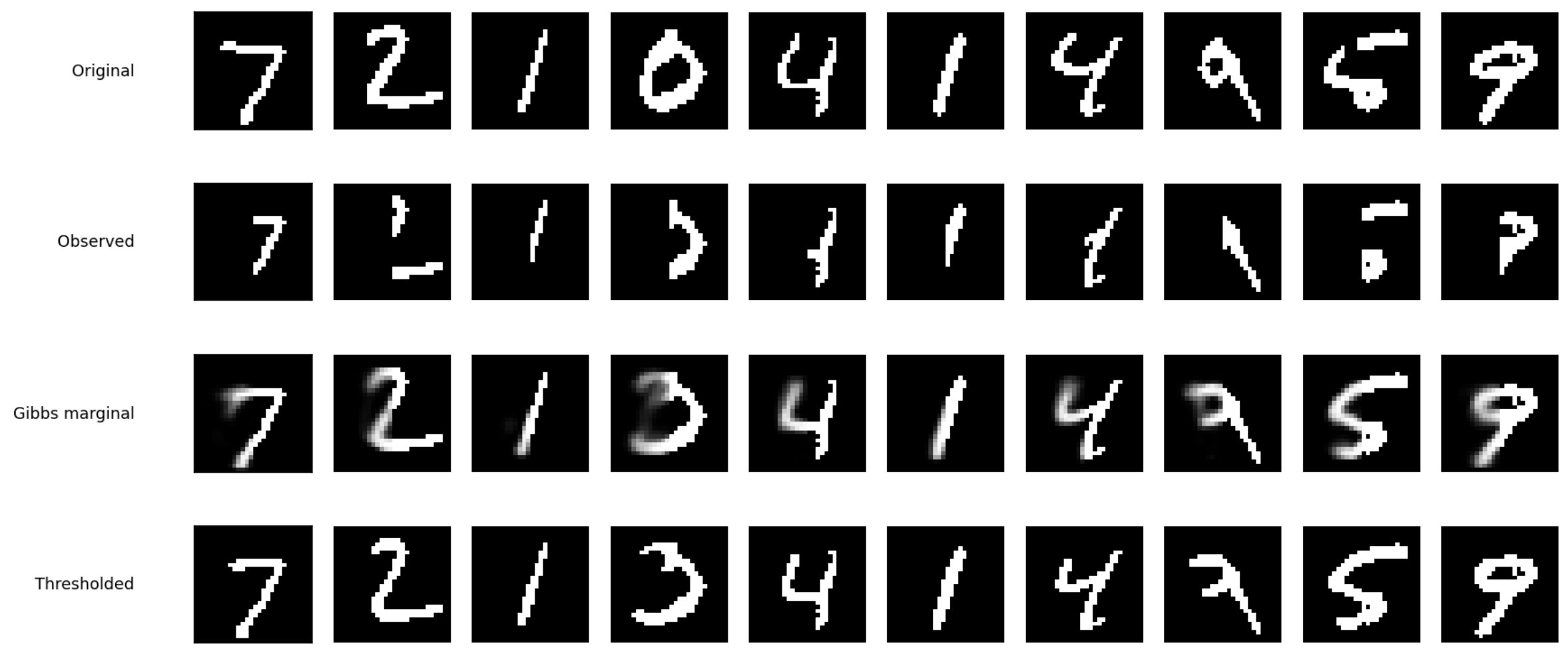
Figure A4.
Completion by the sum-product network on MNIST with the left half hidden. (Top): original. (Second row): the observed half. (Third row): conditional marginals, computed exactly. (Bottom): marginals thresholded at one-half.
Appendix A.2. Convergence of the Partition Function Estimate
Figure A5.
Convergence diagnostics for the annealed importance sampling estimator. (a) Estimated on Fashion-MNIST at 150 epochs across three annealing budgets; error bars are three standard deviations across runs. (b) Effective sample size against the number of Gibbs sweeps. (c) Across-run standard deviation against effective sample size, showing that agreement between runs does not on its own certify the estimate: at an effective sample size of 11% the three runs agreed to within 0.039 nats, while at 21% they differed by 0.096.
References
- LeCun, Y.; Chopra, S.; Hadsell, R.; Ranzato, M.; Huang, F.J. A Tutorial on Energy-Based Learning. In Predicting Structured Data; Bakir, G., Hofmann, T., Schölkopf, B., Smola, A., Taskar, B., Eds.; MIT Press: Cambridge, MA, USA, 2006; Available online: https://cs.nyu.edu/~sumit/publications/assets/ebmtutorial.pdf (accessed on 10 August 2026).
- Hopfield, J.J. Neural Networks and Physical Systems with Emergent Collective Computational Abilities. Proc. Natl. Acad. Sci. USA 1982, 79, 2554–2558. [Google Scholar] [CrossRef] [Scilit] [PubMed]
- Ackley, D.H.; Hinton, G.E.; Sejnowski, T.J. A Learning Algorithm for Boltzmann Machines. Cogn. Sci. 1985, 9, 147–169. [Google Scholar] [CrossRef] [PubMed]
- Smolensky, P. Information Processing in Dynamical Systems: Foundations of Harmony Theory. In Parallel Distributed Processing: Explorations in the Microstructure of Cognition; Rumelhart, D.E., McClelland, J.L., Eds.; MIT Press: Cambridge, MA, USA, 1986; Volume 1, pp. 194–281. [Google Scholar]
- Salakhutdinov, R.; Hinton, G.E. Deep Boltzmann Machines. In Proceedings of the Twelth International Conference on Artificial Intelligence and Statistics; JMLR W&CP: Clearwater Beach, FL, USA, 2009; pp. 448–455. Available online: https://proceedings.mlr.press/v5/salakhutdinov09a.html (accessed on 10 August 2026).
- Fischer, A.; Igel, C. Training Restricted Boltzmann Machines: An Introduction. Pattern Recognit. 2014, 47, 25–39. [Google Scholar] [CrossRef] [Scilit]
- Montúfar, G.F. Restricted Boltzmann Machines: Introduction and Review. In Information Geometry and Its Applications IV; Springer: Cham, Switzerland, 2018; pp. 75–85. Available online: https://link.springer.com/chapter/10.1007/978-3-319-97798-0_4 (accessed on 10 August 2026).
- Neal, R.M. Annealed Importance Sampling. Stat. Comput. 2001, 11, 125–139. [Google Scholar] [CrossRef] [Scilit]
- Poon, H.; Domingos, P. Sum-Product Networks: A New Deep Architecture. In Proceedings of the Twenty-Seventh Conference on Uncertainty in Artificial Intelligence; AUAI Press: Barcelona, Spain, 2011; pp. 337–346. [Google Scholar]
- Sánchez-Cauce, R.; Vázquez-Sánchez, E.; Bielza, C. A Survey on Tractable Probabilistic Models: Representation, Inference, and Learning. Int. J. Approx. Reason. 2021, 133, 1–25. [Google Scholar]
- Xia, R.; Zhang, Y.; Liu, X.; Yang, B. A Survey of Sum–Product Networks Structural Learning. Neural Netw. 2023, 164, 645–666. [Google Scholar] [CrossRef] [Scilit] [PubMed]
- Gens, R.; Domingos, P. Learning the Structure of Sum-Product Networks. In Proceedings of the 30th International Conference on Machine Learning; JMLR W&CP: Atlanta, GA, USA, 2013; pp. 873–880. Available online: https://proceedings.mlr.press/v28/gens13.html (accessed on 10 August 2026).
- MacKay, D.J.C. Information Theory, Inference, and Learning Algorithms; Cambridge University Press: Cambridge, UK, 2003; Available online: https://www.inference.org.uk/itprnn/book.pdf (accessed on 10 August 2026).
- Srivastava, N.; Salakhutdinov, R. Multimodal Learning with Deep Boltzmann Machines. In Advances in Neural Information Processing Systems; Curran Associates, Inc.: Red Hook, NY, USA, 2012; Volume 25, pp. 2222–2230. Available online: https://papers.nips.cc/paper/2012/file/af21d0c97db2e27e13572cbf59eb343d-Paper.pdf (accessed on 10 August 2026).
- Salakhutdinov, R.; Murray, I. On the Quantitative Analysis of Deep Belief Networks. In Proceedings of the 25th International Conference on Machine Learning, Helsinki, Finland, 5–9 July 2008; pp. 872–879. [Google Scholar]
- Sánchez-Cauce, R.; París, I.; Díez, F.J. Sum-Product Networks: A Survey. IEEE Trans. Pattern Anal. Mach. Intell. 2022, 44, 3817–3837. [Google Scholar] [CrossRef] [Scilit] [PubMed]
- Peharz, R.; Gens, R.; Pernkopf, F.; Domingos, P. On the Latent Variable Interpretation in Sum-Product Networks. IEEE Trans. Pattern Anal. Mach. Intell. 2017, 39, 2030–2044. Available online: https://ieeexplore.ieee.org/document/7748514 (accessed on 10 August 2026). [CrossRef] [Scilit] [PubMed]
- Darwiche, A. Modeling and Reasoning with Bayesian Networks; Cambridge University Press: Cambridge, UK, 2009. [Google Scholar]
- Zhao, H.; Melibari, M.; Poupart, P. On the Relationship Between Sum-Product Networks and Bayesian Networks. In Proceedings of the 32nd International Conference on Machine Learning; PMLR: Lille, France, 2015. [Google Scholar]
- Xiao, H.; Rasul, K.; Vollgraf, R. Fashion-MNIST: A Novel Image Dataset for Benchmarking Machine Learning Algorithms. arXiv 2017, arXiv:1708.07747. [Google Scholar] [CrossRef] [Scilit]

Disclaimer/Publisher’s Note: The statements, opinions and data contained in all publications are solely those of the individual author(s) and contributor(s) and not of MDPI and/or the editor(s). MDPI and/or the editor(s) disclaim responsibility for any injury to people or property resulting from any ideas, methods, instructions or products referred to in the content. |
© 2026 by the authors. Licensee MDPI, Basel, Switzerland. This article is an open access article distributed under the terms and conditions of the Creative Commons Attribution (CC BY) license.