Coverage and Precision of Net Promoter Score Confidence Intervals Across Sampling Distributions

Abstract

The Net Promoter Score (NPS) is a widely used metric for customer loyalty in business. However, the current theoretical gaps in the literature suggest practical refinements for real-world applications. In this simulation study, we use an unbiased estimator of the variance for the sample NPS to examine coverage and width for three different confidence interval methods: Wald, bootstrap t, and adjusted Wald with weights corresponding to four underlying population distribution shapes: extreme (E), left-skewed (LS), triangular (T), and uniform (U). As the sample size increased, all methods approached the nominal 95% coverage rate with an exception for the extreme population; the adjusted Wald method with triangular and uniform weights is particularly robust among the representative population shapes examined. All adjusted Wald methods performed comparably in width, especially at a larger n. The confidence interval width depended on the population shape. Overall, the Wald and bootstrap t methods should be avoided at small sample sizes and are not recommended. Our methods raise awareness of the sampling distribution of the NPS statistic, provide a theoretical basis for an unbiased estimator of the variance, and assess reliable confidence interval construction. These results provide an informed application of NPS and lay the foundation for future methodological development.

1. Introduction

The Net Promoter Score (NPS) is a simple but powerful tool used to gauge customer loyalty in business contexts [1]. It is based on one question: “How likely are you to recommend our company/product/service to a friend or colleague?” The responses are given on an 11-point ordinal scale {0, 1, …, 10}, and customers are grouped into three classes: Promoters (those giving 9 or 10), Passives (those giving 7 or 8), or Detractors (those giving 0 up to and including 6). The counts for each of the three classes are taken from a sample survey, and percentages are computed. The NPS is defined to be:

NPS = % Promoters − % Detractors = (proportion of Promoters − proportion of Detractors) × 100.

Without a loss of generality, just the proportions can be used. In this case, we see that the NPS $\in [-1.00,1.00]$. In terms of interpretation, an NPS of 0 means that Promoters and Detractors are proportionally balanced, while positive scores are “good”, demonstrating proportionally more Promoters than Detractors. While there are no widely accepted absolute benchmark values, and these vary among industries, many would consider an NPS over 0.50 to be excellent [2].

The NPS has seen rapid adoption as a key performance indicator of customer loyalty and satisfaction. In practice, organizations track the NPS over time and compare scores across customer segments, making a statistical inference about the NPS (e.g., confidence intervals and hypothesis tests) an important concern. Despite its popularity in business, marketing, healthcare, etc., uncertainty quantification is rarely reported in practice, and guidance on which confidence intervals are reliable for NPS’s categorical nature is limited. The NPS metric has faced scrutiny in the general and peer-reviewed literature. For example, researchers have questioned whether the NPS is truly superior to other customer metrics, with some finding that the NPS typically has no stronger positive association with business outcomes (like customer retention or revenue growth) than other loyalty or satisfaction metrics. Other recent research termed the NPS “ambiguous and unreliable if not accompanied by other tools,” since identical NPS values may mask differing customer sentiment compositions [3]. Rocks [4] gave a brief summary of several of the critiques of the NPS. An extensive and comprehensive historical literature review of the NPS can be found at Measuring U [5].

Because the NPS is so widely used for making strategic decisions across many organizations spanning various sectors, one might question, “how much can we trust this metric?” A way to think about assessing the NPS is to cast its interpretation in the context of estimation under a probability sampling design. For example, suppose that a large healthcare system is considering deploying a workforce development course to its constituents at great expense in terms of time and money. The 10,000 employees represent the population, while 20 individuals attending the inaugural course represent the sample. Hypothetically, if the entire population took the course, the true (and unknown) NPS would be the so-called parameter, using the parlance of a statistician. The NPS computed from the 20 individuals would be the statistic, our point estimate of the parameter. Much like a sampling poll, interest lies in inference on the parameter. How comfortable should leadership be in the system-wide success of the course with the NPS from an inaugural cohort of 20 employees? A single point estimate of NPS with no measure of uncertainty will not be very helpful to the leadership of the healthcare system and could even lead to risky conclusions and decisions. In practice, however, NPS is almost always reported as a single point estimate, with formal measures of uncertainty, such as confidence intervals, rarely if ever given. Providing the leadership with a range of plausible values for the NPS parameter, i.e., a confidence interval, would be useful in making better informed strategic planning, policy making, etc. A confidence interval shifts the NPS from a solitary, potentially misleading number into a more nuanced decision-support tool, enabling organizations to allocate resources, assess initiatives, and gauge risk with greater clarity and conviction.

1.1. Background and Theory

Because it is a difference of two proportions, the NPS itself can be thought of as a statistic derived from a sample from a three-category multinomial distribution (Detractor, Passive, and Promoter counts from a multinomial distribution with three categories). More formally, we have three possible mutually exclusive outcomes, with outcome probabilities $p_{-},p_0$, and $p_{+}$, where these correspond to “success” probabilities for the Detractor, Passive, and Promoter outcomes, respectively. In addition, we assume we have $n\in \{1,2,\dots \}$ independent multinoulli trials, the outcome probabilities are all non-negative, and that $p_{-}+p_0+p_{+}=1$. If the random variables $X_{-},X_0$, and $X_{+}$ indicate the number of times the Detractor, Passive, and Promoter outcomes are observed over the n trials, respectively, then the vector $(X_{-},X_0,X_{+})$ follows a multinomial distribution with parameters n and the vector $(p_{-},p_0,p_{+})$. While the trials are independent, their outcomes, $X_{-},X_0$, and $X_{+}$, are dependent because they must sum to n. The probability mass function for the multinomial distribution in this case is:

$${\displaystyle \frac{n}{x_{-}!x_0!x_{+}!}}{p}_{-}^{x_{-}}{p}_0^{x_0}{p}_{+}^{x_{+}}\mathrm{for}{x}_{-},x_0,x_{+}\ge 0.$$

(1)

Marginally, the count for any single category in a k-category multinomial distribution with a fixed n is binomially distributed:

$$X_i\sim \mathrm{Binomial}(n,p_i)$$

for i = −, 0, or + with probability mass function:

$${\displaystyle \frac{n}{x_i!(n-x_i)!}}{p}_i^{x_i}{(1-p_i)}^{n-x_i}\mathrm{for}{x}_i\ge 0.$$

(2)

Now, suppose we survey a random sample of n respondents. Let $X_{+}\sim \mathrm{Binomial}(n,p_{+})$ and $X_{-}\sim \mathrm{Binomial}(n,p_{-})$. Then, the sample NPS is:

$$\widehat{\mathrm{NPS}}={\displaystyle \frac{X_{+}-X_{-}}{n}}.$$

(3)

We now show important results for this statistic using basic probability theory [6].

Theorem 1.

$\widehat{\mathrm{NPS}}$ is an unbiased estimator for NPS.

Proof. 

Let ${\widehat{p}}_{+}=X_{+}/n$ be the sample proportion of Promoters and ${\widehat{p}}_{-}=X_{-}/n$ be the sample proportion of Detractors. Therefore, $\widehat{\mathrm{NPS}}={\widehat{p}}_{+}-{\widehat{p}}_{-}$.

Hence, the mean, or expected value, of $\widehat{\mathrm{NPS}}$ is:

$$\begin{array}{cc}\hfill \mathrm{E}\left[\widehat{\mathrm{NPS}}\right]& =\mathrm{E}[{\widehat{p}}_{+}-{\widehat{p}}_{-}]\hfill \\ \hfill & =\mathrm{E}\left[{\widehat{p}}_{+}\right]-\mathrm{E}\left[{\widehat{p}}_{-}\right]\hfill \\ \hfill & =p_{+}-p_{-}.\hfill \end{array}$$

□

Theorem 2.

The variance of $\widehat{\mathrm{NPS}}$ for a sample of size n is:

$$\mathrm{Var}\left[\widehat{\mathrm{NPS}}\right]={\displaystyle \frac{p_{+}+p_{-}-{(p_{+}-p_{-})}^2}{n}}.$$

Proof. 

It is known that $\mathrm{Var}\left[{\widehat{p}}_i\right]={\displaystyle \frac{p_i(1-p_i)}{n}}$ for i = − or +, and that $\mathrm{Cov}[{\widehat{p}}_{+},{\widehat{p}}_{-}]=-{\displaystyle \frac{p_{+}{p}_{-}}{n}}$. Hence, the variance of $\widehat{\mathrm{NPS}}$ is:

$$\begin{array}{cc}\hfill \mathrm{Var}\left[\widehat{\mathrm{NPS}}\right]& =\mathrm{Var}[{\widehat{p}}_{+}-{\widehat{p}}_{-}]\hfill \\ \hfill & =\mathrm{Var}\left[{\widehat{p}}_{+}\right]+\mathrm{Var}\left[{\widehat{p}}_{-}\right]-2\mathrm{Cov}[{\widehat{p}}_{+},{\widehat{p}}_{-}]\hfill \\ \hfill & ={\displaystyle \frac{1}{n}}[p_{+}(1-p_{+})+p_{-}(1-p_{-})+2p_{+}{p}_{-}]\hfill \\ \hfill & ={\displaystyle \frac{1}{n}}[p_{+}+p_{-}-{(p_{+}-p_{-})}^2].\hfill \end{array}$$

□

We now consider how to derive an estimator for the variance of $\widehat{\mathrm{NPS}}$.

Theorem 3.

The estimator for the variance of $\widehat{\mathrm{NPS}}$ is:

$${\widehat{\mathrm{Var}}}_1\left[\widehat{\mathrm{NPS}}\right]={\displaystyle \frac{{\widehat{p}}_{+}+{\widehat{p}}_{-}-{({\widehat{p}}_{+}-{\widehat{p}}_{-})}^2}{n}}.$$

The estimator is biased for a small sample size, n, but the bias goes to zero as n becomes large.

Proof. 

Even though $\mathrm{E}\left[{\widehat{p}}_{+}\right]=p_{+}$ and $\mathrm{E}\left[{\widehat{p}}_{-}\right]=p_{-}$, note that $\mathrm{E}\left[{({\widehat{p}}_{+}-{\widehat{p}}_{-})}^2\right]\ne {(p_{+}-p_{-})}^2$. In fact, $\mathrm{E}\left[{({\widehat{p}}_{+}-{\widehat{p}}_{-})}^2\right]=\mathrm{Var}[{\widehat{p}}_{+}-{\widehat{p}}_{-}]+{(p_{+}-p_{-})}^2$. Therefore, the estimator underestimates the true variance and is not correctable in practice. The bias involves the true variance, which is what we are trying to estimate in the first place, making correction circular without additional modeling assumptions. □

While it can be shown that the estimator, as expressed in Theorem 3, is asymptotically unbiased for the variance of $\widehat{\mathrm{NPS}}$, there is an easier way to prove this. Nonetheless, showing this for the estimator as expressed in Theorem 3 may be of some independent interest. We, therefore, include this result in Appendix A.

By simple algebraic rearrangement, we examine an alternative expression of the estimator for the variance of $\widehat{\mathrm{NPS}}$.

Theorem 4.

An alternative expression for the estimator for the variance of $\widehat{\mathrm{NPS}}$ is:

$${\widehat{\mathrm{Var}}}_2\left[\widehat{\mathrm{NPS}}\right]={\displaystyle \frac{{\widehat{p}}_{+}(1-{\widehat{p}}_{+})+{\widehat{p}}_{-}(1-{\widehat{p}}_{-})+2{\widehat{p}}_{+}{\widehat{p}}_{-}}{n}}.$$

The estimator is biased for a small sample size, n, but the bias goes to zero as n becomes large.

Proof. 

From Theorem 2, this estimator directly mimics the form:

$$\mathrm{Var}[{\widehat{p}}_{+}-{\widehat{p}}_{-}]={\displaystyle \frac{[p_{+}(1-p_{+})+p_{-}(1-p_{-})+2p_{+}{p}_{-}]}{n}}.$$

Taking the expectation of ${\widehat{\mathrm{Var}}}_2\left[\widehat{\mathrm{NPS}}\right]$, we compute:

$$\begin{array}{cc}\hfill \mathrm{E}\left[{\widehat{p}}_{+}(1-{\widehat{p}}_{+})\right]& =\mathrm{E}\left[{\widehat{p}}_{+}\right]+\mathrm{E}\left[{\widehat{p}}_{+}^2\right]\hfill \\ \hfill & =p_{+}+\mathrm{Var}\left[{\widehat{p}}_{+}\right]+{\left(\mathrm{E}\left[{\widehat{p}}_{+}\right]\right)}^2\hfill \\ \hfill & =p_{+}-\left({\displaystyle \frac{p_{+}(1-p_{+})}{n}}+p_{+}^2\right)\hfill \\ \hfill & =p_{+}(1-p_{+})\left(1-{\displaystyle \frac{1}{n}}\right)\hfill \end{array}$$

and the result for $\mathrm{E}\left[{\widehat{p}}_{-}(1-{\widehat{p}}_{-})\right]$ is similar. We also see:

$$\begin{array}{cc}\hfill \mathrm{E}\left[2{\widehat{p}}_{+}{\widehat{p}}_{-}\right]& =2(\mathrm{E}\left[{\widehat{p}}_{+}\right]\mathrm{E}\left[{\widehat{p}}_{-}\right]+\mathrm{Cov}[{\widehat{p}}_{+},{\widehat{p}}_{-}])\hfill \\ \hfill & =2\left(p_{+}{p}_{-}-{\displaystyle \frac{p_{+}{p}_{-}}{n}}\right)\hfill \\ \hfill & =2p_{+}{p}_{-}\left(1-{\displaystyle \frac{1}{n}}\right).\hfill \end{array}$$

Accordingly, this gives us the following expression:

$$\mathrm{E}\left[{\widehat{\mathrm{Var}}}_2\left[\widehat{\mathrm{NPS}}\right]\right]=\mathrm{Var}\left[\widehat{\mathrm{NPS}}\right]\ast \left(1-{\displaystyle \frac{1}{n}}\right),$$

(4)

which shows that ${\widehat{\mathrm{Var}}}_2\left[\widehat{\mathrm{NPS}}\right]$ is biased low for $\mathrm{Var}\left[\widehat{\mathrm{NPS}}\right]$. Clearly, the finite-sample correction $\left(1-{\displaystyle \frac{1}{n}}\right)\to 1$ as $n\to \infty$, thus affirming that ${\widehat{\mathrm{Var}}}_2\left[\widehat{\mathrm{NPS}}\right]$ is asymptotically unbiased. □

Theorem 5.

The unbiased estimator for the variance of $\widehat{\mathrm{NPS}}$ is:

$${\widehat{\mathrm{Var}}}_3\left[\widehat{\mathrm{NPS}}\right]={\displaystyle \frac{{\widehat{p}}_{+}(1-{\widehat{p}}_{+})+{\widehat{p}}_{-}(1-{\widehat{p}}_{-})+2{\widehat{p}}_{+}{\widehat{p}}_{-}}{n-1}}.$$

Remark 1.

The estimated standard deviation of $\widehat{\mathrm{NPS}}$ is simply ${\widehat{\mathrm{SD}}}_3\left[\widehat{\mathrm{NPS}}\right]=\sqrt{{\widehat{\mathrm{Var}}}_3\left[\widehat{\mathrm{NPS}}\right]}$.

Proof. 

This estimator is merely a bias-corrected version of the alternative expression of the estimator given in Theorem 4, using a known multiplicative factor. The derivation immediately follows by multiplying both sides of Equation (4) by $n/(n-1)$. □

1.2. Confidence Intervals for NPS

Confidence intervals for the difference between independent proportions have been well studied (e.g., see [7]). To derive a confidence interval for NPS, which is the difference between two dependent proportions, there are three approaches we can take.

First, we can compute Wald confidence intervals under the assumption of approximate normality for $\widehat{\mathrm{NPS}}$ as:

$$\begin{array}{c}\hfill \widehat{\mathrm{NPS}}\pm z_{1-\alpha /2}^{*}·\sqrt{{\widehat{\mathrm{Var}}}_3\left[\widehat{\mathrm{NPS}}\right]},\end{array}$$

(5)

where $z_{1-\alpha /2}^{*}$ is the $1-\alpha /2$ quantile of the standard normal distribution, and ${\widehat{\mathrm{Var}}}_3\left[\widehat{\mathrm{NPS}}\right]$ is the unbiased estimator for the variance of $\widehat{\mathrm{NPS}}$ from Theorem 5. Wald confidence intervals for NPS are simple and reasonable in moderate-to-large sample sizes but can be too narrow in small samples, especially when ${\widehat{p}}_{+}$ or ${\widehat{p}}_{-}$ is near the boundary 0 or 1. This is due to the reliance on the normal approximation and poor variance estimation at boundaries. In fact, it is possible that Wald confidence intervals can extend beyond the boundaries −1 or 1, which is not valid for NPS.

An important work that addressed large-sample confidence intervals for pairwise comparisons of multinomial proportions was given by Goodman [8]. Goodman used the (biased) variance given in Theorem 2, along with the square root of the $1-\alpha /M$ quantile of the ${\chi }^2$ distribution with 1 degree of freedom for $\alpha \in [0,1]$. This is a Bonferroni correction on the ${\chi }^2$ critical point to adjust for the $M=k(k-1)/2$ possible pairwise differences available across all k categories. In our case, since NPS was pre-specified, and we are not interested in the other two pairwise differences, we use $M=1$, and Goodman’s method reduces to a Wald confidence interval (note the square root of the $1-\alpha$ quantile of the ${\chi }^2$ distribution with 1 degree of freedom is equivalent to the $1-\alpha /2$ quantile of the standard normal distribution).

Second, we can compute bootstrapped confidence intervals when we have small sample sizes and the assumption of normality for $\widehat{\mathrm{NPS}}$ is tenuous. There are several different types of nonparametric bootstrap confidence intervals that we can consider, including the bootstrap percentile interval and the t interval with bootstrap standard error, for example. Efron and Tibshirani [9] described “confidence intervals based on bootstrap tables”, also commonly referred to as studentized bootstrap intervals or bootstrap t confidence intervals. While bootstrapping does not overcome the weakness of small samples as a basis for inference, Hesterberg [10] showed that bootstrap t confidence intervals can perform relatively well compared to the other confidence interval types, with respect to coverage, width, and robustness when n is small. Bootstrap t confidence intervals could work well for NPS because there is no reliance on the normal approximation, and the procedure will account for the skewness of the sampling distribution and heteroskedasticity with respect to $\widehat{\mathrm{NPS}}$. Also, bootstrap t confidence intervals fully account for the dependence between ${\widehat{p}}_{+}$ and ${\widehat{p}}_{-}$ because we are resampling across all observations. Bootstrapping assumes the empirical distribution approximates the population well, which can be suspect if n is very small.

Rocks [4] proposed and systematically evaluated several interval estimation techniques for NPS via simulation and empirical data. One finding was that the Wald confidence interval performed poorly. By contrast, so-called “adjusted” Wald (AW) confidence intervals (simply adding a pseudo-count to each category before generating a Wald confidence interval) provided substantial improvements in accuracy. A well-performing method that was identified was a specific adjusted Wald variant denoted as AW(3, T) (we will describe this notation in greater detail in Section 2). This method involves adding 3/4 to the counts of both Promoters and Detractors and 3/2 to the count of Passives before the construction of a Wald confidence interval. AW(3, T) achieved the lowest mean absolute error in coverage among several methods and “good performance across the n values and confidence levels examined, especially for data likely to be observed in practice.”

When we incorporate pseudo-counts, this leads to an adjusted sample size and adjusted proportions, which means we are working with a different estimator, that is, a smoothed version of $\widehat{\mathrm{NPS}}$, denoted as ${\widehat{\mathrm{NPS}}}_s$. The adjusted Wald method uses ${\widehat{\mathrm{NPS}}}_s$, not the original $\widehat{\mathrm{NPS}}$, as the center of the confidence interval. While the smoothed estimator can be biased for the true NPS, this is intentionally done to improve the behavior of the confidence interval. Note that ${\widehat{\mathrm{Var}}}_3\left[\widehat{\mathrm{NPS}}\right]$ is only unbiased for the variance of the original NPS estimator based on the original multinomial sample of size n. If we apply the AW(3, T) confidence interval with the estimator in Theorem 5 using the adjusted sample size and adjusted proportions, then it is important to recognize that ${\widehat{\mathrm{Var}}}_3\left[{\widehat{\mathrm{NPS}}}_s\right]$ will be unbiased only for the variance of ${\widehat{\mathrm{NPS}}}_s$. Also, it can be shown that the variance of ${\widehat{\mathrm{NPS}}}_s$ (using Theorem 2) will generally be smaller than the variance of $\widehat{\mathrm{NPS}}$, with the difference depending on the alignment of the prior multinomial distribution implied by the added pseudo-counts and the true outcome probabilities. More will be said about this in Section 2. The key takeaway is that the adjusted Wald method sacrifices the accuracy of the estimator (bias) for the sake of a relatively larger gain in precision (smaller variance), a classic bias–variance tradeoff.

When considering our confidence interval approaches, one of the first questions we must answer is, “When will approximate normality hold for the sampling distribution of $\widehat{\mathrm{NPS}}$?” The sampling distribution of $\widehat{\mathrm{NPS}}={\widehat{p}}_{+}-{\widehat{p}}_{-}$ will begin to look approximately normal as the sample size increases because it is the difference between two (correlated) binomial sample proportions. This relies on an extension of the classic binomial normal approximation rule, which is a specific application of the Central Limit Theorem, and it allows us to state that each expected count for the Promoter and Detractor multinomial cells should be at least 5, with 10 being better [11].

So, a rough rule of thumb in practice to determine whether $\widehat{\mathrm{NPS}}$ is approximately normal would be:

$$\begin{array}{c}\hfill min(n{\widehat{p}}_{+},n{\widehat{p}}_{-})\ge 5(\mathrm{preferably}\ge 10\mathrm{for}\mathrm{a}\mathrm{better}\mathrm{approximation}).\end{array}$$

(6)

For example, if ${\widehat{p}}_{+}=0.80$ and ${\widehat{p}}_{-}=0.10$, then at $n=50$, the sampling distribution for $\widehat{\mathrm{NPS}}$ would be borderline normal since $n{\widehat{p}}_{+}=X_{+}=40$ and $n{\widehat{p}}_{-}=X_{-}=5$. This works because both ${\widehat{p}}_{+}$ and ${\widehat{p}}_{-}$ are binomial proportions (based on marginals of a multinomial) and the difference of two approximately normal random variables is also approximately normal. It can be shown that the two binomial sample proportions’ being correlated only affects the variance of the limiting distribution, not its normality.

1.3. Value Added from Our Approach

After reviewing the scope and limitations of the current literature on the NPS, we identify several unresolved inferential issues and provide a focused, statistically grounded critique that motivates the methodological contributions developed in this paper. While some existing work, most notably Rocks [4], has proposed several confidence interval methods and sparked interest in inference for NPS, important questions remain underexplored.

Understanding the sampling distribution of $\widehat{\mathrm{NPS}}$ is crucial for assessing inference quality. This includes exploring its actual shape or behavior conditional on various multinomial distributions. The sampling distribution is discrete and bounded, with symmetry or skewness depending on the underlying outcome probabilities. Simulating from multiple multinomial distributions and directly visualizing the sampling distributions of $\widehat{\mathrm{NPS}}$ yields crucial insight (e.g., visualizing sampling variability).

As a corollary, we provide diagnostic guidance for when the sampling distribution of $\widehat{\mathrm{NPS}}$ is approximately normal. The Wald method relies heavily on the approximate normality of the sampling distribution. In small samples, the sampling distribution of $\widehat{\mathrm{NPS}}$ could be far from normal, so ignoring this jeopardizes interval coverage and hypothesis test validity.

Bootstrap methods offer a flexible approach that is standard in modern practice. Specifically, bootstrap t confidence intervals are easy to implement and offer a nonparametric alternative for highly discrete or skewed settings, especially for small sample sizes.

The estimator of $\mathrm{Var}\left[\widehat{\mathrm{NPS}}\right]$ commonly used in the literature is biased, as we rigorously demonstrate in this paper. This could negatively impact confidence interval performance assessments, especially for small sample sizes. We derive and employ a finite-sample unbiased variance estimator that is not standard in the existing NPS inference, using it for our assessment of each confidence interval method under consideration.

In confidence interval assessments, precision matters as much as coverage. Accordingly, we examine both coverage and width. This is a key point because two intervals may both attain nominal 95% coverage, say, but have different precisions. Focusing on coverage and width provides a fuller picture of interval performance.

Studies often focus on the marginal (averaged) performance of estimation over the parameter space. However, when employing an inference in practice, we primarily focus on performance conditional on a single observed or assumed multinomial distribution that is emblematic of real-world data settings. Averaging over many multinomial distributions can mask poor performance in specific but important cases (e.g., very high NPS).

The performance of the adjusted Wald method is sensitive to the choice of pseudo-counts, which implicitly encode prior beliefs about the underlying multinomial distribution. If the parameterization for the actual distribution of counts is far from the implied prior used to determine the adjusted counts, then the estimate of NPS could be substantially biased, and the difference in variances between smoothed and unsmoothed estimators of the NPS could be substantially impacted. Therefore, the resulting confidence interval may achieve poor coverage or inflated width. This risk is important to characterize and understand.

Taken together, the points above represent a set of distinct methodological and practical contributions to inference for the NPS:

• We characterize and visualize the finite-sample sampling distribution of $\widehat{\mathrm{NPS}}$ under realistic multinomial response profiles, demonstrating when normal approximations are unreliable and why this directly affects confidence interval validity.
• We show that the variance estimator commonly used for NPS inference is biased in finite samples and introduce a finite-sample unbiased variance estimator, using it to reassess confidence interval performance across methods.
• Rather than averaging performance over the parameter space, we evaluate confidence interval methods conditional on realistic data-generating scenarios, jointly considering coverage and width to provide actionable guidance for robust interval selection in practice.

These contributions motivate the simulation and analytical results that follow, which are designed to quantify the coverage, precision, and robustness of competing confidence interval procedures under realistic finite-sample conditions.

Section 2 describes the data-generating framework, variance estimators, and confidence interval methods under study. Section 3 presents simulation results assessing finite-sample coverage and width across realistic scenarios, and Section 4 discusses these findings in the context of applied settings.

2. Materials and Methods

This section formally defines the confidence interval procedures and populations under consideration evaluated in the simulation study.

To compute bootstrap t confidence intervals, we resample the studentized statistic:

$$t^{*}={\displaystyle \frac{{\widehat{\mathrm{NPS}}}^{*}-\widehat{\mathrm{NPS}}}{{\widehat{\mathrm{SD}}}_3^{*}}},$$

which is the defining feature of the bootstrap t method, where:

• $\widehat{\mathrm{NPS}}$ = the estimate from the original sample
• ${\widehat{\mathrm{NPS}}}^{*}$ = the bootstrap estimate from the bootstrap sample (resampled with replacement)
• ${\widehat{\mathrm{SD}}}_3^{*}$ = estimated standard deviation of ${\widehat{\mathrm{NPS}}}^{*}$ from the bootstrap sample using Theorem 5.

To construct the confidence interval, for each bootstrap sample, $b=1,2,\dots ,B$, we compute $t^{*}$. For each simulated dataset, we used $B=1000$ bootstrap samples. Random number generation was initialized using a fixed seed to ensure reproducibility. We next obtain $t_{1-\alpha /2}^{*}$ and $t_{\alpha /2}^{*}$, which are quantiles of the B values of $t^{*}$. The bootstrap t interval is:

$$\begin{array}{c}\hfill [\widehat{\mathrm{NPS}}-t_{1-\alpha /2}^{*}·{\widehat{\mathrm{SD}}}_3\left[\widehat{\mathrm{NPS}}\right],\widehat{\mathrm{NPS}}-t_{\alpha /2}^{*}·{\widehat{\mathrm{SD}}}_3\left[\widehat{\mathrm{NPS}}\right]],\end{array}$$

(7)

where ${\widehat{\mathrm{SD}}}_3\left[\widehat{\mathrm{NPS}}\right]$ is the estimated standard deviation from the original sample using Theorem 5. Note that, for all confidence interval methods considered in this paper, no truncation to the natural bounds of the NPS ([−1, 1]) was applied. This choice was made to ensure a fair comparison across methods and to avoid introducing method-specific distortions in coverage or the interval width. In our simulations, we observed no evidence of degenerate bootstrap samples causing the collapse of the bootstrap t interval. In particular, bootstrap t interval widths were never near zero. Accordingly, no special handling or filtering of near-zero variance bootstrap samples was required.

Following Rocks [4], we use the notation AW(w, shape) to denote an adjusted Wald confidence interval, where w is the total weight added across the observed counts, and shape describes the assumed distribution of outcome probabilities corresponding to a population that is either extreme (E), triangular (T), or uniform (U). We also introduce a population that is left-skewed (LS), a shape likely to be observed in the field. In our research, w is set equal to 3. Details are given below in

Table 1. Populations Under Consideration.

Population	Pseudo-Counts	$({\mathit{p}}_{-},{\mathit{p}}_0,{\mathit{p}}_{+})$	Variance
Extreme	(3/2, 0, 3/2)	(1/2, 0, 1/2)	1.00
Left-Skewed	(1/4, 1/4, 5/2)	(1/12, 1/12, 5/6)	0.35
Triangular	(3/4, 3/2, 3/4)	(1/4, 1/2, 1/4)	0.50
Uniform	(1, 1, 1)	(1/3, 1/3, 1/3)	0.67

. Each population configuration serves as a fixed data-generating mechanism from which repeated samples are drawn to induce a sampling distribution for $\widehat{\mathrm{NPS}}$, allowing us to study finite-sample variability and departures from normality under realistic response profiles.

To compute adjusted Wald confidence intervals, we first consider the pseudo-counts added to the original vector of counts $(X_{-},X_0,X_{+})$, respectively. For example, for AW(3, LS) we would have $(X_{-}+1/4,X_0+1/4,X_{+}+5/2)$. Notice all pseudo-counts sum to $w=3$ for each population, so that the “sample size” used to compute the adjusted Wald confidence interval is equal to $n+3$. By dividing the pseudo-counts by 3, we obtain the implied prior distribution of outcome probabilities. Notice that the three populations E, T, and U have vectors $(p_{-},p_0,p_{+})$, such that the NPS = 0. However, the left-skewed population with vector $(p_{-},p_0,p_{+})=(1/12,1/12,5/6)$ has a NPS = $5/6-1/12=0.75$. The variance (of $\widehat{\mathrm{NPS}}$) listed in Table 1 is for a single multinoulli trial using the formula given in Theorem 2.

We use simulation ($100,000$ draws) to obtain twelve sampling distributions of $\widehat{\mathrm{NPS}}$ associated with different populations using different sample sizes. With $R=100,000$ replications per scenario, the maximum Monte Carlo standard error for coverage estimates is $\sqrt{0.25/R}\approx 0.0016$, making simulation variability negligible for the comparisons of interest. For each of the four populations in Table 1, we use sample sizes of $n=20,50,100$. In this research, the confidence coefficient C will be set to 0.95. For each sample, we compute a Wald confidence interval using Equation (5), and a bootstrap t confidence interval using Equation (7). We also compute four adjusted Wald confidence intervals; specifically, AW(3, E), AW(3, LS), AW(3, T), and AW(3, U). As described previously, this simply means using pseudo-counts and, subsequently, the adjusted sample size and adjusted proportions, to obtain ${\widehat{\mathrm{NPS}}}_s$ and ${\widehat{\mathrm{Var}}}_3\left[{\widehat{\mathrm{NPS}}}_s\right]$ (using Theorem 5), which are then input into Equation (5). Critically, for each of the four populations, three of the adjusted Wald confidences will be misspecified to the extent that the implied prior distribution of outcome probabilities will not align with the true distribution of outcome probabilities for the population from which the sample were drawn. We then compute the average width and proportion coverage of the confidence intervals across the 100,000 samples from the four populations for each sample size and for all six confidence interval types. Note that coverage will be computed with respect to the respective true NPS for each population.

Lastly, we generate three visuals. First, we generate a faceted plot of the twelve sampling distributions of $\widehat{\mathrm{NPS}}$. Second, we generate a line plot of coverage rates that shows how often the six different 95% confidence intervals contain the true NPS across different sample sizes and populations. This evaluates empirical coverage. Third, we generate a line plot of average interval widths that displays the average width of the 95% confidence intervals for each method, again by sample size and population. This reflects the precision and efficiency of the intervals.

All analyses were performed using R Statistical Software (v4.4.2; R Core Team 2024) [12]. The code to reproduce our analysis is openly available at (https://github.com/philturk/Net_Promoter_Score_Confidence_Intervals, accessed on 15 April 2026).

3. Results

Using the methods and range of realistic data-generating scenarios defined in Section 2, we now evaluate the sampling distribution and finite-sample confidence interval coverage and width associated with the estimation of NPS.

3.1. Sampling Distributions of $\widehat{\mathrm{NPS}}$

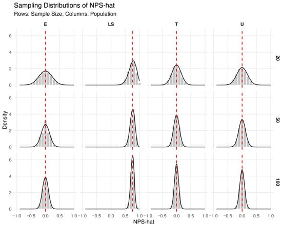
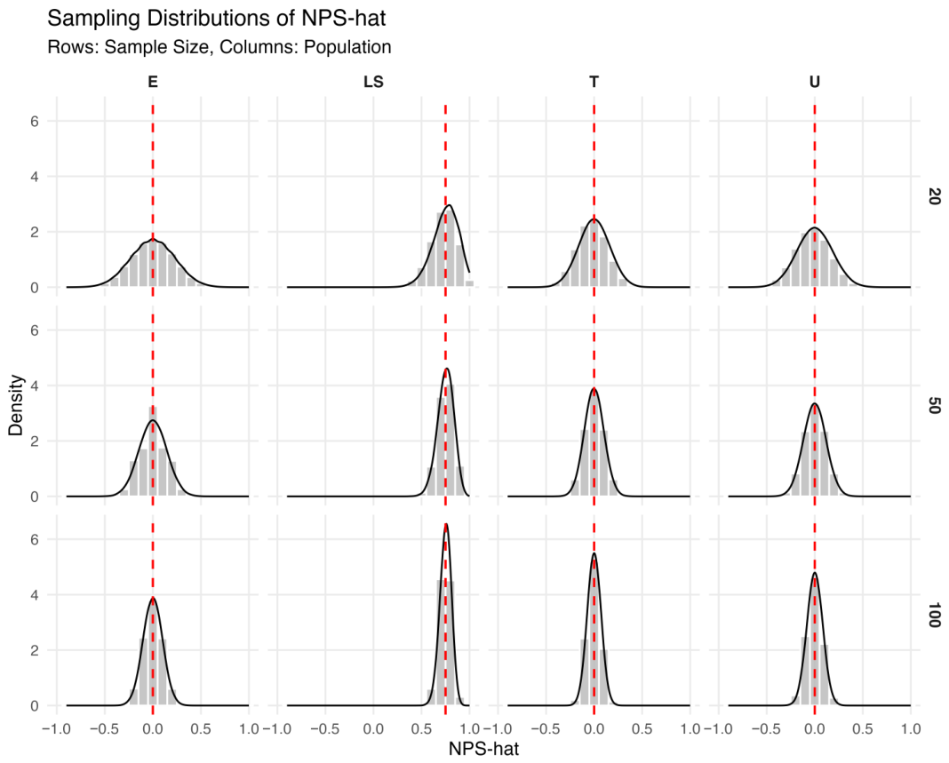
The sampling distributions of $\widehat{\mathrm{NPS}}$ are displayed in Figure 1. These sampling distributions represent the distribution of $\widehat{\mathrm{NPS}}$ obtained from repeated samples drawn from a fixed population configuration in Table 1 and illustrate when approximate normality is plausible and when it fails. The red dashed vertical lines represent the true NPS for each of the populations. Notice that the mean of each sampling distribution approximately equals the true NPS (unbiasedness). For the left-skewed population, the sampling distributions corresponding to $n=20$ and, to a lesser extent, $n=50$ show non-normality. These are conditions under which the rule of thumb given in Equation (6) would not hold. Not surprisingly, the extreme population shows the greatest variance. Notice that the variability could be substantial for smaller sample sizes. This could have a dramatic effect on decision making for leaders who use NPS.

3.2. Confidence Interval Coverage

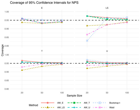
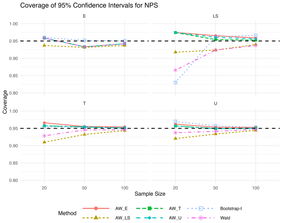
Looking at Figure 2, we see that the simulation results depend on the sample size and population. Correctly matching the adjusted Wald variant to the corresponding population type provides no guarantee that one will attain the specified confidence interval coverage. For example, AW(3, LS) yields confidence intervals that are too narrow and performs no better, or sometimes even worse, than the three other adjusted Wald variants. In general, as n increases, all six methods yield confidence intervals with coverage closer to the advertised 95%. Note that the extreme population is an exception since it is a boundary case on the multinomial simplex ($p_0=0$), which induces a highly discrete sampling distribution for $\widehat{\mathrm{NPS}}$ (grid spacing $2/n$) and maximal variance. Because NPS can only take values on this coarse grid, confidence interval coverage cannot adjust smoothly and instead exhibits oscillatory behavior as n changes, particularly near the boundary of the NPS scale. These features together slow the apparent finite-sample convergence of empirical coverage toward the nominal level. We see that, in the absence of prior knowledge and among the population shapes examined, AW(3, T) and AW(3, U) are good choices for a confidence interval method, followed closely by AW(3, E). The Wald and AW(3, LS) methods cannot be recommended as sensible choices generalizable over all n and population types.

To complement the graphical summaries in Figure 2,

Table 2. Mean empirical coverage (nominal 95%) across population shapes (E, LS, T, U) and sample sizes $n\in \{20,50,100\}$.

Method	E			LS			T			U
	20	50	100	20	50	100	20	50	100	20	50	100
Wald	0.958	0.933	0.942	0.866	0.924	0.937	0.928	0.945	0.946	0.937	0.941	0.947
Bootstrap t	0.960	0.952	0.951	0.830	0.963	0.966	0.955	0.953	0.951	0.970	0.957	0.953
AW(3,E)	0.958	0.933	0.942	0.975	0.965	0.959	0.966	0.955	0.954	0.962	0.953	0.953
AW(3,LS)	0.937	0.931	0.937	0.918	0.924	0.940	0.910	0.932	0.944	0.920	0.934	0.944
AW(3,T)	0.958	0.933	0.942	0.974	0.954	0.953	0.957	0.954	0.951	0.957	0.949	0.950
AW(3,U)	0.958	0.933	0.942	0.975	0.961	0.956	0.957	0.954	0.951	0.957	0.949	0.950

reports mean empirical coverage across all population shapes, sample sizes, and confidence interval procedures.

3.3. Confidence Interval Width

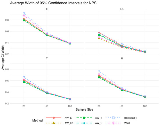
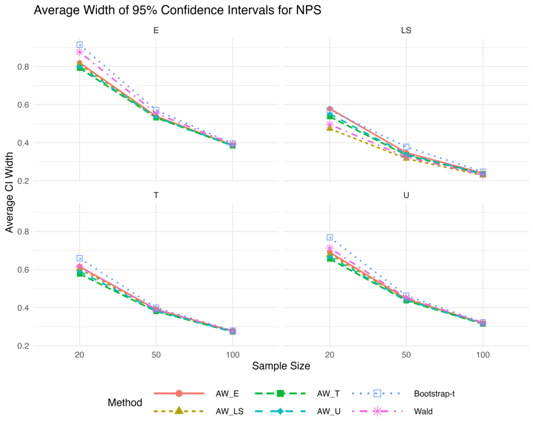
The simulation results for the average width of the 95% confidence intervals in Figure 3 also depend on the sample size and population. The extreme population gave the broadest confidence intervals, while the left-skewed population gave the narrowest. Looking over population types at $n=20$, and also comparing back to the coverage in Figure 2, reveals that the Wald and bootstrap t methods should be avoided. The adjusted Wald methods are fairly comparable in width for each population types, especially as n gets bigger.

Corresponding numerical summaries of mean confidence interval width are reported in

Table 3. Mean confidence interval width across population shapes (E, LS, T, U) and sample sizes $n\in \{20,50,100\}$.

Method	E			LS			T			U
	20	50	100	20	50	100	20	50	100	20	50	100
Wald	0.876	0.554	0.392	0.496	0.325	0.232	0.615	0.391	0.277	0.713	0.452	0.320
Bootstrap t	0.914	0.571	0.395	0.570	0.378	0.247	0.659	0.400	0.279	0.769	0.463	0.323
AW(3,E)	0.819	0.539	0.386	0.579	0.347	0.240	0.615	0.391	0.277	0.690	0.446	0.318
AW(3,LS)	0.810	0.537	0.386	0.473	0.316	0.228	0.603	0.388	0.276	0.679	0.443	0.317
AW(3,T)	0.791	0.531	0.383	0.537	0.335	0.235	0.577	0.380	0.273	0.656	0.436	0.314
AW(3,U)	0.801	0.533	0.384	0.551	0.339	0.237	0.590	0.384	0.274	0.667	0.439	0.315

, allowing a direct comparison of precision across methods and sample sizes.

3.4. Applied Illustration

To reinforce how small-sample inference can differ across interval constructions, we consider a simple worked example motivated by the LS population in Table 1. Suppose a survey of size $n=20$ yields counts:

$$(X_{-},X_0,X_{+})=(1,2,17),$$

which is consistent with an LS setting. Clearly, the normal approximation is questionable. The sample proportions are ${\widehat{p}}_{+}=17/20=0.85$ and ${\widehat{p}}_{-}=1/20=0.05$, giving:

$$\widehat{\mathrm{NPS}}={\widehat{p}}_{+}-{\widehat{p}}_{-}={\displaystyle \frac{17-1}{20}}=0.80.$$

We first compute the Wald confidence interval. Using the finite-sample unbiased variance estimator from Theorem 5, we obtain:

$${\widehat{\mathrm{Var}}}_3\left[\widehat{\mathrm{NPS}}\right]={\displaystyle \frac{0.85\left(0.15\right)+0.05\left(0.95\right)+2\left(0.85\right)\left(0.05\right)}{19}}={\displaystyle \frac{0.2600}{19}}\approx 0.01368,$$

so ${\widehat{\mathrm{SD}}}_3\left[\widehat{\mathrm{NPS}}\right]\approx \sqrt{0.01368}=0.117$. A nominal 95% Wald interval (Equation (5)) is therefore:

$$0.80\pm 1.96\left(0.117\right)=[0.571,1.029].$$

In this illustration, the interval extends beyond the natural parameter space for NPS, which is bounded above by 1.

Next, consider the adjusted Wald procedure AW(3, T), which adds pseudo-counts $(3/4,3/2,3/4)$ to $(X_{-},X_0,X_{+})$. This yields adjusted counts:

$$(X_{-}^{*},X_0^{*},X_{+}^{*})=(1.75,3.5,17.75),n^{*}=n+3=23,$$

and adjusted proportions ${\widehat{p}}_{+}^{*}=17.75/23$ and ${\widehat{p}}_{-}^{*}=1.75/23$. The smoothed NPS estimator is:

$${\widehat{\mathrm{NPS}}}_s={\widehat{p}}_{+}^{*}-{\widehat{p}}_{-}^{*}={\displaystyle \frac{17.75-1.75}{23}}={\displaystyle \frac{16}{23}}\approx 0.696.$$

Applying the same unbiased variance estimator (Theorem 5) with the adjusted sample size gives:

$${\widehat{\mathrm{Var}}}_3\left[{\widehat{\mathrm{NPS}}}_s\right]\approx 0.01654,{\widehat{\mathrm{SD}}}_3\left[{\widehat{\mathrm{NPS}}}_s\right]\approx 0.129,$$

and thus a nominal 95% adjusted Wald interval:

$$0.696\pm 1.96\left(0.129\right)=[0.444,0.948].$$

Compared to the Wald interval, AW(3, T) is slightly wider in this example, but it remains within $[-1,1]$ (n.b., as with any normal-approximation interval, adjusted Wald intervals can also extend beyond the parameter bounds in small samples). This simple illustration aligns with the simulation findings for the LS population at small n; specifically, while Wald intervals can be narrower in this setting, adjusted Wald procedures (e.g., AW(3, T)) provide more stable inference under discreteness and skewness. Because AW(3, U) behaved similarly to AW(3, T) in our simulations, we omit it here for brevity.

4. Discussion

There are limitations we acknowledge in this research. In practice, the assumption that we have obtained a true simple random sample might be plainly suspect. Quite often, we are dealing with a representative sample or, perhaps, a voluntary response sample. Nevertheless, our methods give practitioners a benchmark that could be useful, provided that any interpretation is tempered with caution.

To complement the coverage and width results, we briefly examine the bias of the NPS estimators at $n=20$. As expected, the original estimator $\widehat{\mathrm{NPS}}$ and the bootstrap-based approach exhibit a negligible degree of bias across all population configurations. In contrast, the smoothed estimator underlying adjusted Wald intervals can exhibit non-negligible bias when the implied pseudo-count distribution is misaligned with the true population, with a magnitude approaching 0.10 in our simulations. When the pseudo-counts are well aligned with the underlying population, the bias is effectively zero. These results highlight the bias–variance tradeoff inherent to adjusted Wald methods; improved coverage and stability may come at the cost of bias under model misspecification.

As mentioned in Section 1, an NPS value of zero represents a natural interpretive benchmark separating Promoter and Detractor subpopulations. In practice, testing whether NPS differs from zero aligns with how the metric would be used in organizational benchmarking and decision-making. For hypothesis testing (e.g., checking if a NPS is significantly different from zero or if two NPS scores differ), we note that similar principles apply. Because $\widehat{\mathrm{NPS}}$ is essentially a sample mean (of coded values $-1,0$, and 1), a one-sample t-test can test if NPS equals zero, or some other value under the null hypothesis, by using the estimated standard deviation and $n-1$ degrees of freedom. In practice, this would be a useful tactic for assessing whether customer loyalty to a product, say, is comparable to that of some predefined standard. Likewise, comparing two independent NPS scores (from, say, two companies or two time periods) can be done with a two-sample t statistic comparing the difference in $\widehat{\mathrm{NPS}}$ to zero. For example, a two-sample t-test of NPS scores of a product or service over a period of time is a way to assess whether a statistically significant improvement in customer loyalty has been achieved. These procedures assume approximate normality of the NPS estimator, an assumption that can be checked using our rule of thumb. The main caution is to use the correct variance formula for NPS and not to treat the two proportions (${\widehat{p}}_{+}$ and ${\widehat{p}}_{-}$) as if they were independent.

A line of inquiry we have explored in our research has been to raise awareness about the sampling distribution of the NPS statistic and to more rigorously address its inferential properties. Because $\widehat{\mathrm{NPS}}$ is a linear combination of multinomial counts, its exact sampling distribution is discrete (with a granularity of $1/n$ in NPS units), being derived from the multinomial probability mass function. Our results confirm that the uncertainty in $\widehat{\mathrm{NPS}}$ can be considerable, leading to confidence intervals for NPS that can be very wide for small sample sizes. Overall, while NPS is valued for simplicity, we caution against over-reliance on a single-number metric without proper statistical context and validation when making an inference about a customer base.

Sampling variability in $\widehat{\mathrm{NPS}}$ is something that should not be ignored. Much like high-quality sampling polls, the recommendation we make is to always pair an estimate of NPS with a margin of error or confidence interval. However, in practice, the authors note that this is rarely done. The consequences of ignoring sampling variability can be practically profound and lead to “chasing noise”. Let us reconsider our example with the healthcare system that is considering deploying a new workforce development course to its constituents. Consider a scenario under which, had all the constituents taken the course (the population), the true unknown NPS would have been 0.75. Now, suppose a class consists of 20 students. On average, we would expect $\widehat{\mathrm{NPS}}\approx 0.75$, and yet, it is entirely possible by chance to see an estimate of 0.25 (Figure 1). The leadership at the healthcare system might wrongly conclude that the course is ineffective when, in fact, the healthcare system at large would enthusiastically embrace the course. As a second scenario, it is possible that a population could have a true unknown NPS of 0, and yet, a class of 20 students might yield an estimate of 0.50 due to chance (Figure 1). The leadership at the healthcare enterprise might wrongly conclude that the course is excellent when, on average, all of their constituents actually view the course with equanimity.

Many times in practice, there might be neither intuition nor prior knowledge as to the type of population under consideration. Based on our simulation results for the coverage and width of confidence intervals for NPS that account for the multinomial nature of the data, the adjusted Wald methods with triangular or uniform pseudo-counts are good choices across a range of practically relevant population shapes, followed by extreme pseudo-counts.

The mean squared error (MSE) of an estimator is defined to be the sum of the variance of the estimator and the squared bias of the estimator. This provides a useful way to compare estimators with respect to precision and accuracy to see which one is “best”, at least from an MSE perspective. We did not compute the MSEs for the alternative and unbiased estimators for $\mathrm{Var}\left[\widehat{\mathrm{NPS}}\right]$. As expected, the smoothed estimator for NPS underlying adjusted Wald intervals exhibits finite-sample bias when the implied pseudo-count distribution is misaligned with the true population, particularly at very small sample sizes. However, the inferential consequences of this bias are already captured through the empirical coverage results reported here. A systematic evaluation of estimator bias and MSE represents a natural direction for future work.

Our methods are developed assuming an infinite, or “large”, population. If samples are drawn from a finite population, such that the sampling fraction becomes excessively high (e.g., ≥0.10, say), then the resulting confidence intervals for NPS using the methods given in our research will be conservative. Future research could explore attenuating the variance estimator using a finite-population correction factor [13].

In practice, when we have missing data or nonresponse (e.g., 10 out of 20 students in a class respond to a survey), our treatment of the issue depends on the reason for the missingness and our analysis goals. Practical approaches for resolving the issue depend on the setting and can become quite complex. This would represent another fruitful area of future research. A complete case analysis, the most common approach, assumes that responses are missing completely at random and proceeds with estimation using just the respondents. However, there is a risk of bias in estimation if the nonrespondents differ systematically from the respondents, which occurs when missingness is not completely at random. When in doubt, seek the consultation of a trained statistician.

References

- Reichheld, F.F. The one number you need to grow. Harv. Bus. Rev. 2003, 81, 46–55. [Google Scholar] [PubMed]
- Qualtrics. What Is a Good Net Promoter Score? 2021. Available online: https://www.qualtrics.com/experience-management/customer/good-net-promoter-score/ (accessed on 4 July 2025).
- Cazzaro, M.; Chiodini, P.M. Statistical validation of critical aspects of the Net Promoter Score. TQM J. 2023, 35, 191–209. [Google Scholar] [CrossRef] [Scilit]
- Rocks, B. Interval estimation for the “net promoter score”. Am. Stat. 2016, 70, 365–372. [Google Scholar] [CrossRef] [Scilit]
- Measuring U. Has the Net Promoter Score Been Discredited in the Academic Literature? 2019. Available online: https://measuringu.com/nps-discredited/#:~:text=Across%2022%2...emic%20papers%2C%20we,best%20predictor%2C%20it%20was%20close (accessed on 4 July 2025).
- Casella, G.; Berger, R.L. Statistical Inference, 2nd ed.; Duxbury: Pacific Grove, CA, USA, 2002. [Google Scholar]
- Newcombe, R.G. Interval estimation for the difference between independent proportions: Comparison of eleven methods. Stat. Med. 1998, 17, 873–890. [Google Scholar] [CrossRef] [Scilit]
- Goodman, L.A. On Simultaneous Confidence Intervals for Multinomial Proportions. Technometrics 1965, 7, 247–254. [Google Scholar] [CrossRef]
- Efron, B.; Tibshirani, R. An Introduction to the Bootstrap; Chapman and Hall/CRC: New York, NY, USA, 1993. [Google Scholar]
- Hesterberg, T.C. What teachers should know about the bootstrap: Resampling in the undergraduate statistics curriculum. Am. Stat. 2015, 69, 371–386. [Google Scholar] [CrossRef] [Scilit] [PubMed]
- Ott, L.; Longnecker, M. An Introduction to Statistical Methods and Data Analysis; Cengage Learning: Boston, MA, USA, 2016. [Google Scholar]
- R Core Team. R: A Language and Environment for Statistical Computing; R Foundation for Statistical Computing: Vienna, Austria, 2024. [Google Scholar]
- Thompson, S.K. Sampling, 3rd ed.; Wiley Series in Probability and Statistics Sampling; Wiley: Hoboken, NJ, USA, 2012. [Google Scholar]
Disclaimer/Publisher’s Note: The statements, opinions and data contained in all publications are solely those of the individual author(s) and contributor(s) and not of MDPI and/or the editor(s). MDPI and/or the editor(s) disclaim responsibility for any injury to people or property resulting from any ideas, methods, instructions or products referred to in the content. |
© 2026 by the authors. Licensee MDPI, Basel, Switzerland. This article is an open access article distributed under the terms and conditions of the Creative Commons Attribution (CC BY) license.