


Abstract
This paper presents a linear mathematical model of bass guitar string vibration with experimentally identified, frequency- and fret-dependent modal damping, aimed at high-fidelity generative sound synthesis. To identify the string damping parameters across various frets and configurations, an experimental framework was developed to benchmark four structural identification methods: half-power bandwidth, I. Yoshida’s method, Discrete Fourier Transform Interpolation, and Hilbert-transform envelope approximation. Experiments were systematically conducted on Cort C4H, Ibanez RB 630, and Yamaha bass guitars. Based on the extracted parameter space, two audio generation strategies are formulated: a spectrum-driven harmonic reconstruction method (Method 1) and a physical modeling approach utilizing spatial wave equations (Method 2). The proposed linear approximation framework effectively captures the inverse relationship between the damping factor and fret numbers specifically on the E-string, while mapping linear increases on the G and D-strings. Quantitative verification using Sobolev norm differences demonstrates good agreement between the synthesized and original signals for the spectrum-driven method (Q = 0.031–0.057) and moderate agreement for the physics-based wave equation method (Q = 0.058–0.153). This reflects a trade-off in which the former achieves tighter spectral convergence, while the latter better preserves the physical, time-domain waveform structure. As both synthesis strategies are closed-form and computationally lightweight, the model is suitable for real-time implementation and the dynamic control of playing techniques (e.g., plucking location and, in principle, slap-type excitation), without relying on heavy, multi-gigabyte audio sample libraries.
1. Introduction
Today, the creation of musical compositions increasingly relies on virtual instruments and synthesized audio environments [1]. Implementing a traditional sampling approach requires a comprehensive library containing every sound that a musical instrument can reproduce across various dynamics and articulations [1]. Such high-quality sound sample libraries occupy significant storage space and demand substantial time and financial investment to create; for instance, a complete set of high-fidelity bass guitar sounds can easily take up to 7–8 GB [1]. In the context of modern cloud-based and mobile music production technologies, there is an urgent demand for lightweight and efficient alternatives, which has shifted the research focus toward generative audio synthesis based on physical models [1]. Developing mathematical models that generate musical instrument sounds taking into account the mechanical properties of the string and specific playing techniques is, therefore, of great practical and theoretical importance [1].
A substantial body of work has been devoted to creating the sound of stringed musical instruments using various physical modeling frameworks [1,2]. General wave equations for different instruments have been thoroughly examined in the classical literature [1]. However, while lossless wave models are well understood, accurate timbre replication and sound naturalness depend heavily on the precise characterization of energy dissipation and damping properties [2,3]. In recent years, researchers have focused extensively on passive space–time-domain modeling of frequency-dependent losses in linear strings, where losses at low frequencies are governed by air viscosity and internal friction dominates at higher frequencies [3]. Accurate numerical implementation requires energy-stable time-stepping and finite-difference schemes, particularly when incorporating non-linear contact effects and collisions with frets or obstacles [4,5]. Moreover, contemporary studies have successfully applied complex modal bases and reduced-order models to capture multi-dimensional wave propagation and viscothermal losses without prohibitive computational costs [4]. Linear synthesis formulations have also proven effective in reproducing the systematic decay rate patterns observed in instruments with strong string-body coupling [6].
A major challenge in physical modeling synthesis remains the accurate identification of the friction and damping parameters, which are difficult to calculate from purely analytical principles due to the complex viscoelastic behavior of the string material and its construction [2,3]. To address this, combined experimental and information-driven methods have emerged. Advanced signal processing techniques, including the modified Hilbert-Huang transform, empirical mode decomposition, and fast interpolated discrete-time Fourier transform (IpDTFT) estimators utilizing maximum sidelobe decay windows, are now deployed to extract instantaneous frequencies and damping factors from noisy structural vibration data with high precision [7,8]. Concurrently, there is a prominent trend toward hybrid approaches that combine governing physical equations with artificial neural networks [9,10,11]. Recent implementations include GPU-accelerated finite-difference methods, differentiable modal synthesis [10], and convolutional neural networks designed for parameter estimation and real-time optimization of virtual string designs [11,12]. Additional insights into structural damping estimation have also been derived from ambient and environmental vibration techniques using geophones and piezoelectric sensors [9,13].
While various physical modeling paradigms exist, each presents a trade-off between physical accuracy and computational cost. Digital waveguide modeling, introduced fundamentally for string instruments [14] and continuously advanced in recent comprehensive and impedance-based formulations [15,16], is widely used for real-time synthesis due to its extreme computational efficiency. Yet, accurately calibrating its digital filters to match the precise frequency-dependent damping of specific guitar frets remains challenging. On the other end of the spectrum, finite-difference time-domain (FDTD) string models [4,5,17] provide rigorous accuracy and successfully capture complex non-linear fret collisions. However, despite recent algorithmic advances for real-time guitar synthesis [17], FDTD methods are typically computationally prohibitive for lightweight, multi-channel synthesis without dedicated hardware acceleration. Furthermore, advanced modal synthesis approaches and related relaxation techniques [4,10,18] effectively handle complex boundary conditions and non-linearities but often rely on generalized or idealized damping coefficients. Frequency-dependent damping formulations [3] have improved time-domain linear strings, yet a direct mapping of these losses across changing fret positions remains underdeveloped. In contrast to these methods, the proposed approach serves as a highly efficient middle ground. By integrating an explicit linear analytical model with an experimentally extracted, fret-dependent damping framework, the computational bottleneck of non-linear FDTD solvers is avoided while achieving greater physical parameter transparency than standard digital waveguides.
To address the limitations of standard structural identification under environmental noise and varying boundaries, researchers often employ specialized techniques such as the half-power bandwidth method [19,20], internal friction torsional pendulums [21], or discrete mechanical spectroscopy algorithms [22]. However, a direct bridge between these structural damping extraction techniques and lightweight, real-time synthesis engines remains underdeveloped, especially for multi-channel sampled environments [23] and rigorous error metrics based on Sobolev norms [24].
The primary objective of this work is to bridge the gap between rigorous structural damping extraction and lightweight, real-time synthesis by developing a robust method for generating the sound of an electric bass guitar with specified characteristics based on the analytical string vibration equation [1]. Unlike complex non-linear simulations, a linear engineering approach is proposed where the damping parameter is evaluated as a function of frequency and fret positions. To achieve this, a specialized parameter identification algorithm was developed by combining and benchmarking four distinct spectral and temporal estimation techniques [19,20,21,22]. The proposed approach was validated using experimental recordings from three commercially available bass guitar architectures (Cort C4H, Ibanez RB 630, and Yamaha bass), providing a highly controllable, closed-form synthesis framework whose low computational cost makes it suitable for real-time response to playing techniques, without reliance on heavy, multi-gigabyte audio sample libraries [1,23].
To make the relationship between this work and the literature on physical modeling and modal damping explicit, the specific contributions of this study relative to prior work are as follows:
- Benchmarking of damping-identification methods in a new application domain. While the half-power bandwidth [19,20], torsional-pendulum internal friction [21], and interpolated-DFT estimation [22] methods have each been developed and validated individually, this has occurred largely in non-musical structural-engineering contexts (e.g., buildings, timber poles, and torsion pendulums). To the best of our knowledge, this is the first study to combine and directly benchmark four independent estimators—half-power bandwidth, I. Yoshida’s method, DFT interpolation, and Hilbert-transform envelope approximation—specifically for electric bass guitar strings, across multiple frets, strings, and three distinct instrument architectures.
- A fret-indexed empirical damping law. While frequency-dependent damping formulations for linear strings are well established [3], a direct, experimentally derived mapping of these losses across discrete fret positions has yet to be reported. This work provides such a fret-indexed damping model, calibrated per string for three commercially representative bass guitars, spanning both passive (Ibanez) and active (Cort) pickup designs.
- An explicit middle ground between existing synthesis paradigms. Digital waveguide models achieve real-time efficiency but require ad hoc filter tuning to approximate frequency-dependent damping [14,15,16]; FDTD and complex-modal formulations capture non-linear behavior with high fidelity, but at a computational cost that is prohibitive for lightweight or multi-channel synthesis [4,5,10,17,18]. The proposed linear engineering model is closed-form and computationally trivial while retaining direct physical parameter transparency, thereby filling a niche not directly served by either paradigm.
- Quantitative, ground-truth-based comparison of two synthesis strategies. Both the spectral parametric reconstruction (Method 1) and the physics-based wave equation synthesis (Method 2) are compared, for the first time in this context, against the same experimentally recorded signals using a rigorous Sobolev-norm similarity criterion [24], rather than being evaluated in isolation or through informal listening alone.
Together, these elements distinguish the present work from both prior sample-based synthesis, which depends on multi-gigabyte sound libraries [1,23], and prior physically accurate but computationally heavy models. This is achieved by providing a lightweight, closed-form, dynamically controllable (e.g., pluck position and, in principle, slap-type excitation) synthesis method that is suitable for real-time use and grounded in experimentally validated, instrument-specific damping data.
2. Mathematical Modeling and Experimental Methods
2.1. String Vibration Model
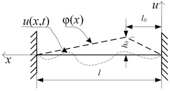
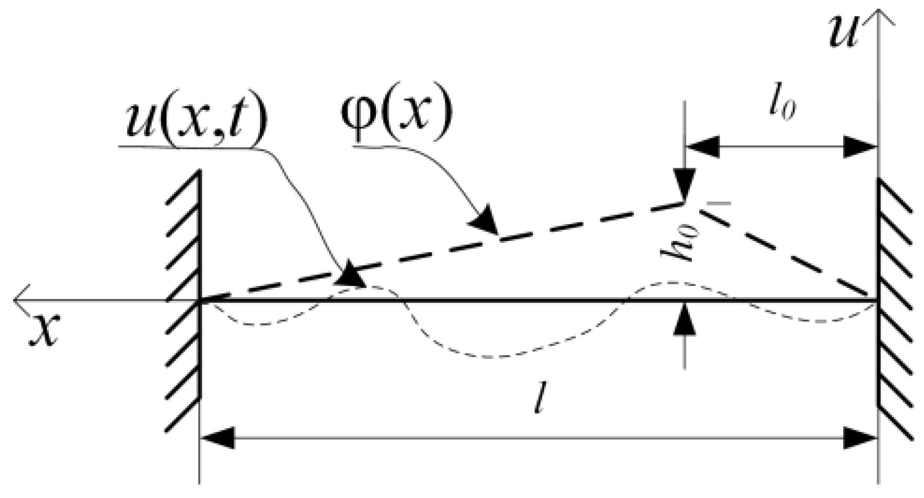
We propose using the classical linear model of string vibration with friction (1), initial conditions (2), and boundary conditions (3). The friction force function is denoted as ε(x, t). The boundary and initial conditions are schematically shown in Figure 1. In this work, we chose a model that does not take into account the flexural rigidity of the string, since according to the results obtained in [25], the effect of flexural rigidity on the vibration frequencies does not exceed 0.53%. Furthermore, while advanced passive space–time-domain methods have been developed to capture complex energy dissipation under geometric non-linearities, a linear model with modal damping remains highly sufficient for a solid-body electric bass guitar. This is due to the fact that string displacements after a standard plucking initialization rapidly stabilize within the linear elastic range, making computationally expensive non-linear structural solvers unnecessary for real-time sound synthesis frameworks.
Figure 1.
Model string, boundary and initial conditions.
We use the following notation:
u(x,t)—string displacement function,
x—coordinate along string,
t—time,
φ(x)—initial displacement of string,
ψ(x)—initial velocity of string,
l—string length,
l0—pluck point,
p—fundamental frequency, , where T is string tension and ρ is linear density;
The solution to Equation (1) is presented in the following form:
The form of expression (4) is selected based on the method of eigenmode decomposition. The form of function (5) corresponds to the modal damping model. Substituting (4) and (5) into Equation (1) we obtain:
Here, k = 1, 2, … denotes the harmonic (mode) number, and ωk~ is the corresponding angular frequency of the k-th mode.
This leads to the following equations:
The solution of the second equation of the system is the equation:
The solution of the first equation of the system is:
In practice, ; therefore, in applications is often assumed. The parameter p depends on the string material and tension force. Its value is chosen in such a way that the frequency of the first harmonic corresponds to the given one. , where ν is the frequency of the first harmonic in Hz.
By combining the solutions, we obtain
where the coefficients ak and bk are determined from the initial conditions and can be expressed as follows:
For plucked musical instruments, the initial conditions are recorded based on the method of picking. In such musical instruments, the initial displacement of the string by the value h0 at the point l0 is set (Figure 1), while the initial velocity of the string is zero. Mathematically, this can be written in the form of expressions (16), (17). The linear form of the dependence of the string on the x-coordinate follows from the solution of Equation (1) with the rejected inertial terms (static deflection).
Substituting expressions (16) and (17) into (14) and (15) yields the analytical dependence of the coefficients ak and bk on the string excitation point l0.
As can be seen from (18) and (19), the coefficients ak and bk depend linearly on the magnitude of the initial displacement h0. Because this coefficient is essentially responsible for sound volume, we assume h0 = 1 to simplify the model, meaning that volume control can be carried out through the linear scaling solutions.
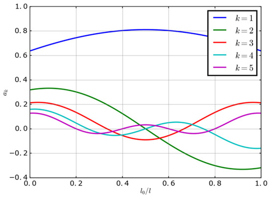
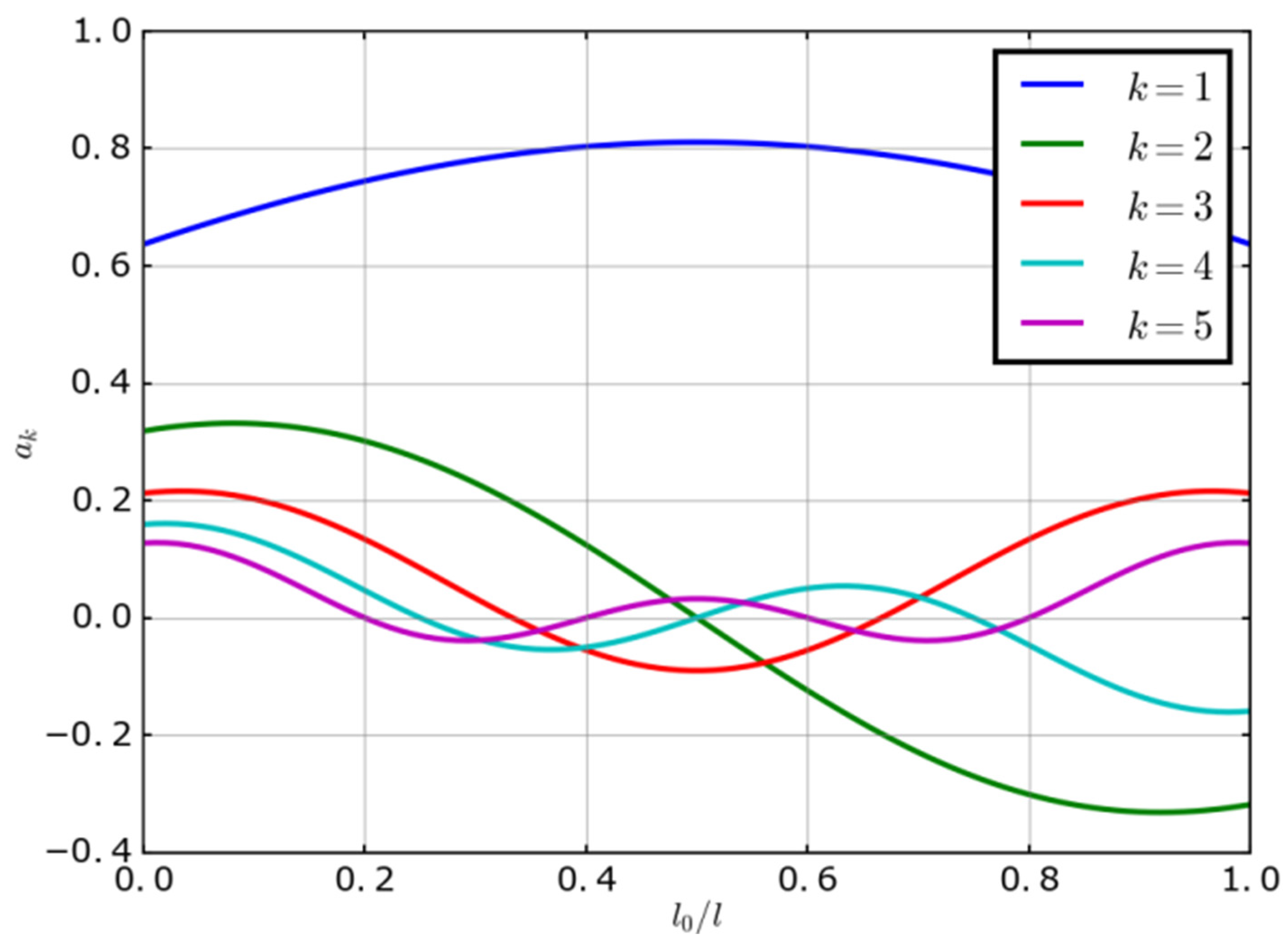
The coefficient l0 allows for the control of the timbre. Figure 2 shows the dependence of the coefficient ak on the string excitation point l0 relative to the string length l. As can be seen from the figure, when the string excitation point is closer to the edge of the string, the higher harmonics exhibit a greater amplitude and hence a sharper timbre. In the case of string excitation closer to its center, the amplitudes of higher harmonics decrease, leading to a softer timbre due to the predominance of the first harmonic.
Figure 2.
Dependence of the coefficient ak on the string excitation point l0/L.
By combining all the elements, the solution to the vibration equation for a bass guitar string with modal damping and pinch string excitation can be written as follows:
It should be noted that the assumption ψ(x) = 0 for plucked musical instruments may not always hold, particularly under certain playing styles. To simulate such a situation, we propose setting the function ψ(x) in the following form:
where s0 is the parameter responsible for the impulse width, m; and υ0 is the value of the initial velocity, m/s.
By substituting (24) into (15), the corresponding coefficients bk can be found. To find the value of bk, an analytical expression can be obtained, but it is very cumbersome and requires the use of special functions and complex variables. This makes its use comparable in complexity with the numerical integration of the expression. It is worth noting, however, that in contemporary musical acoustics and wave simulation, such analytical constraints and high computational costs of numerical integration for complex boundary velocities are increasingly bypassed using hybrid methodologies. Recent trends favor leveraging artificial neural networks and differentiable modal synthesis to accelerate graphics processing unit solvers or directly predict multi-dimensional wave motion under non-zero velocity profiles. Nevertheless, to preserve a transparent engineering structure, this study maintains the formalized assumption ψ(x) = 0, relying on the benchmarking of traditional estimation routines.
To calculate Equation (20), it is necessary to determine the constants εk, which are responsible for the damping properties of the string. These parameters have a complex physical nature and may differ from instrument to instrument; hence, we propose to determine them experimentally.
2.2. Evaluation Methods for Damping Parameters
To determine the damping parameters of the string, we propose employing a set of methods. While all these methods allow for obtaining the values of the damping parameters in different scenarios, they demonstrate different error rates. A rather broad overview of such methods is presented in [19]. According to the recommendations of that study, four methods were selected:
- -
- The half-power-bandwidth method [20];
- -
- The method proposed by I. Yoshida [21];
- -
- The Hilbert transform-based envelope approximation method [9];
- -
- The interpolated discrete fourier transform method (IpDFT) [22].
2.2.1. The Half-Power Bandwidth Method
The half-power bandwidth method is based on a spectral analysis of string vibrations and the estimation of peak widths. To obtain the spectrum, the DFT is used (25).
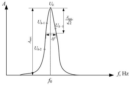
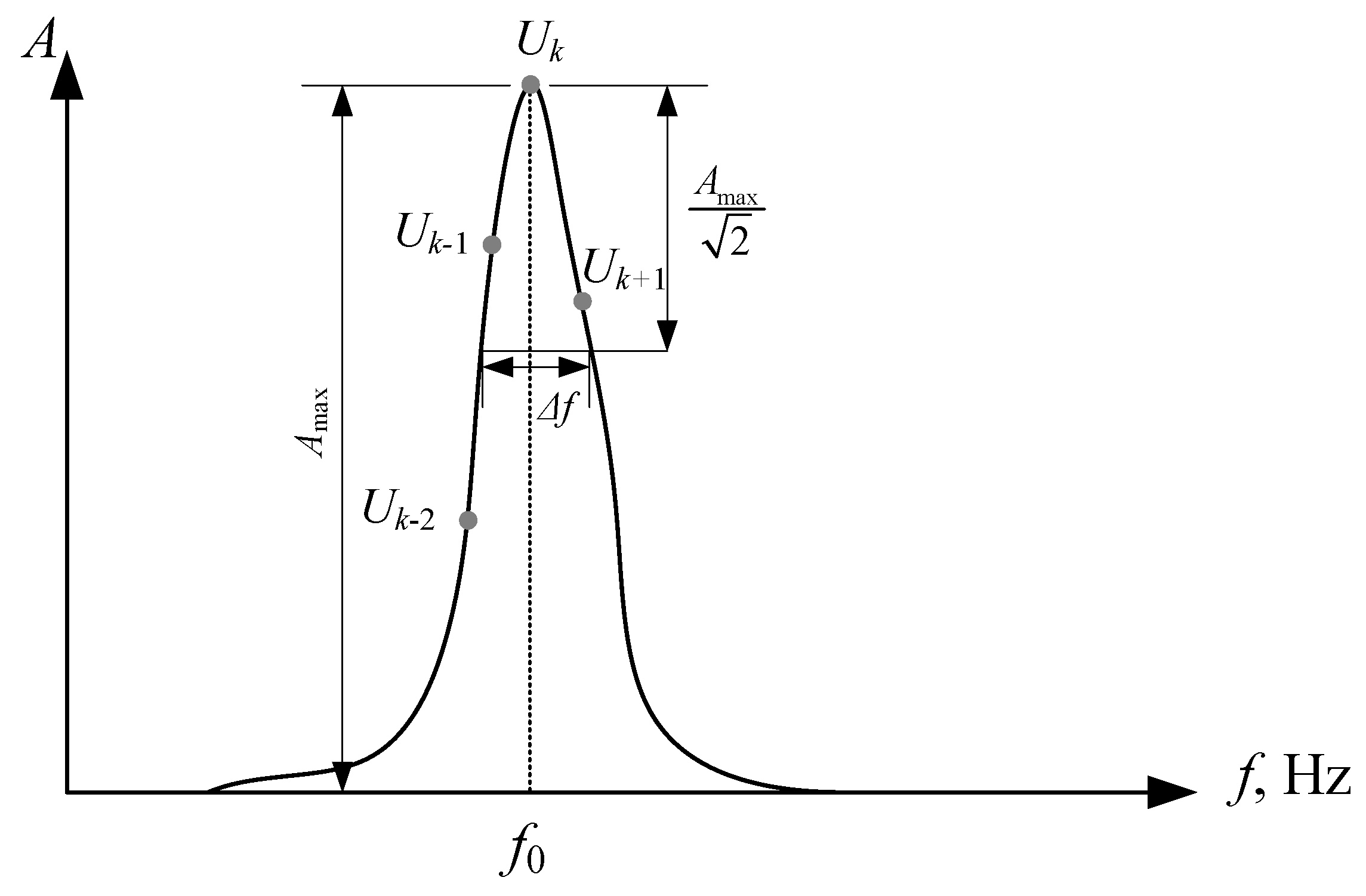
The spectrum of a string vibration process typically exhibits a peak. Its schematic representation is shown in Figure 3. According to this method, the peak width Δf is located at a height of 1/√2 from Amax. So, it is possible to determine the main parameters of the damping system: the damping parameter (ε), the logarithmic damping decrement, etc.
Figure 3.
Typical peak on signal spectrum.
It is important to note a key characteristic of non-stationary signal analysis using the FFT: the value of Amax in the spectrum corresponds to the average value of the amplitude of the analyzed signal. To obtain the true amplitude of the signal, it is proposed to use Equation (27).
2.2.2. The Yoshida Method
The method proposed by I. Yoshida is based on the idea of representing the signal as the sum of three components: the main component of the damped oscillation, a parasitic motion, and a residual component not included in the first two. Further, a discrete Fourier transform is performed on these signals. The unknown constants are determined from the substitution of points of the real spectrum into the expression describing the spectrum of the three functions. Thus, the essence of the method is reduced to the calculation of two expressions:
where Uk−2… Uk+1 are points of the spectrum of the discrete Fourier transform around the peak.
2.2.3. The Interpolated Discrete Fourier Transform Method (IpDFT)
The interpolation method of the discrete Fourier transform is conceptually similar to the previous method. However, the spectrum is interpolated by polynomials, and the spectrum is calculated using the Hanning window. According to this method, two variables, R1 and R2, are introduced based on which the damping parameters are calculated.
2.2.4. The Hilbert Transform-Based Envelope Approximation Method
The Hilbert transform-based envelope approximation method is based on the idea of obtaining an analytical signal using the Fourier and Hilbert transforms. In the case of a discrete signal, conversion to an analytical form can be performed using the following expression:
where Uk is the signal spectrum obtained using the DFT (25);
According to the property of an analytical signal, the unsa envelope can be found as its modulus (35).
The decay signal envelope in a semi-logarithmic coordinate system is a straight line
where the parameters ε and ε0 are determined using the least squares method.
2.3. Parameter Extraction Algorithm
The vibrations of the strings are complex and polyharmonic. Such vibrations can be represented as a sum of harmonic functions. Each k-th harmonic of the series is characterized by four parameters: amplitude (Ak), frequency (ωk), phase (φk) and damping (εk). To describe the entire vibration process, it is necessary to define 4k parameters.
To isolate harmonics from a polyharmonic signal, the authors proposed the following algorithm.
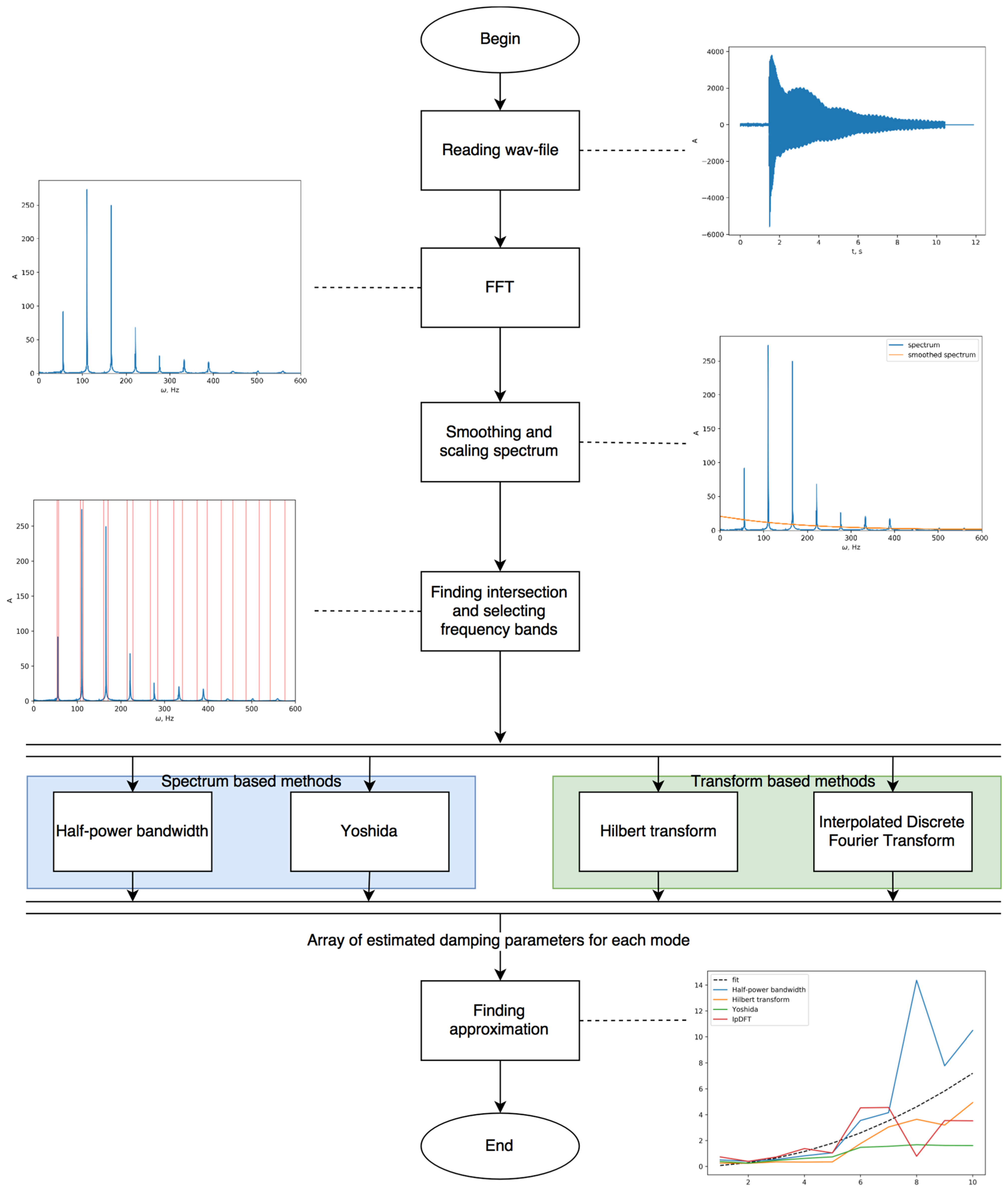
Step 0. Reading the file with the recorded sound;
Step 1. Calculating the discrete Fourier transform;
Step 2. Smoothing the obtained spectrum. Smoothing the spectrum produces a curve that is similar to the average noise level in the signal and does not contain useful harmonics. To improve the algorithm, the smoothed curve can be scaled to 0.05–0.15 of the amplitude of the maximum harmonic.
Step 3. Finding the intersections of the smoothed and the original spectra. The intersection points delineate frequency bands that correspond to the peaks in the spectrum.
Step 4. Determining the frequency and phase of the harmonics. The frequency and phase are determined directly from the spectrum.
Step 5. Determining the damping parameters. The damping parameter is determined using four methods: the half-power bandwidth method, I. Yoshida’s method, the Hilbert transform-based envelope approximation method, and the interpolation method of the discrete Fourier transform (see Section 2.2). To obtain a more reliable estimate of the damping parameters, the results are averaged.
No single one of the four estimators is uniformly the most accurate: each rests on different assumptions and has a distinct bias–variance behavior and failure mode. The half-power bandwidth method, for instance, is robust to noise but sensitive to closely spaced or overlapping peaks and to record length, whereas the Yoshida and interpolated-DFT methods are highly precise on clean spectra but use only a few spectral bins around each peak and are correspondingly noise-sensitive. Because the ground-truth damping of a real recording is unknown, the unweighted mean of the four estimates is used as a deliberately conservative central value: it avoids privileging the assumptions of any single method and reduces the influence of any one method’s systematic error. As quantified in Section 3.1, this choice is well justified in the high-SNR regime of the controlled recordings used here (23–25 dB), where all four estimators agree to within sub-percent error (Table 1); its behavior at lower SNR, where the average inherits the error of the least-robust contributing method, is analyzed in detail there.
Table 1.
Parameters of the original (Src) and recovered signal (Est).
Step 6. Determining the amplitude of the harmonic. The initial amplitude of the harmonic is calculated using Equation (27).
Steps 4–6 are repeated for each harmonic.
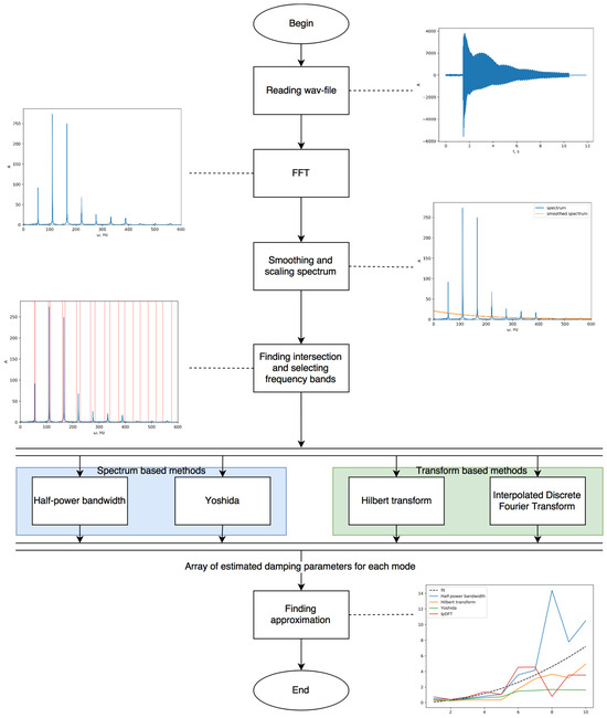
A visual representation of the algorithm is shown in Figure 4.
Figure 4.
The algorithm for determining the parameters of the string vibrations.
3. Results and Discussion
3.1. Algorithm Testing on Synthetic Signals
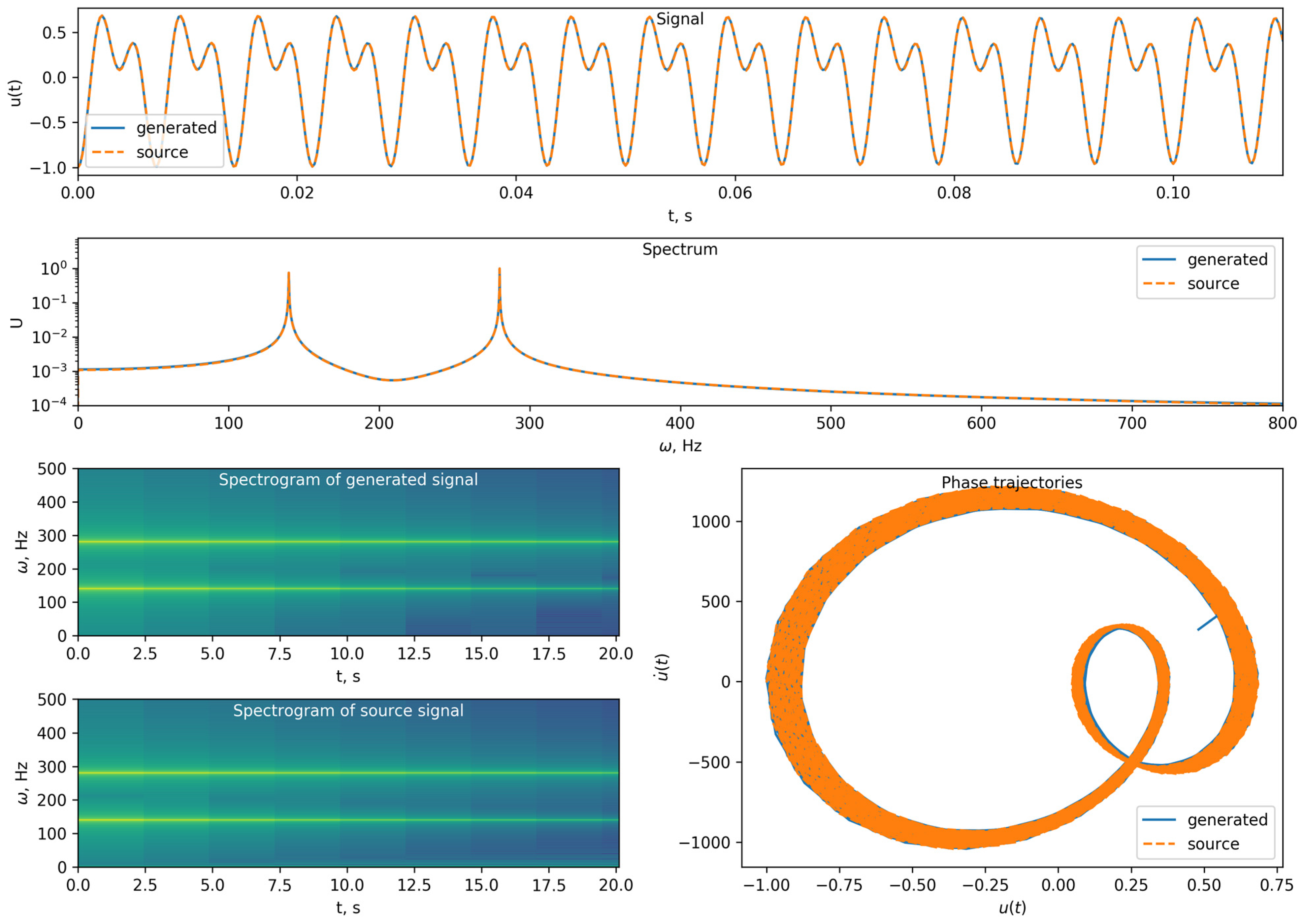
To test the correctness of the developed algorithm, a signal with previously known characteristics has been generated. For this analysis, the test signal is defined as follows:
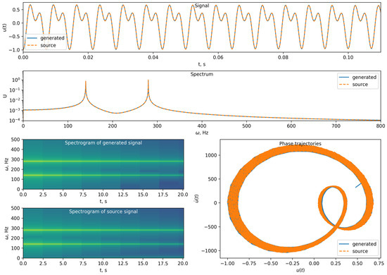
The above algorithm has been applied to this signal. The results of the algorithm are shown in Table 1. Based on the extracted parameters, the signal has been reconstructed (Figure 5).
Figure 5.
Comparison of the original and recovered signal. Colors on the spectrum shows signal amplitude.
The damping coefficients εk reported in Table 1 are obtained as the unweighted average of four independent estimators: the half-power (−3 dB) spectral bandwidth method, the Hilbert-transform envelope log-slope method, the Yoshida three-point interpolated-DFT method, and the interpolated-DFT method with M = 1 (IpDFT). To characterize the reliability of this averaging procedure under realistic recording conditions, the noise term A0·rand(t) in Equation (38) was varied systematically, and its effect on each of the four estimators was quantified separately, rather than only on their combined average.
The noise level is expressed as a signal-to-noise (SNR) ratio,
where urms is the root-mean-square value of the noise-free signal u(t) over the analysis window. For each SNR value in the range −6 to +40 dB, 20 independent noise realizations (zero-mean Gaussian) were generated, and the relative estimation error (%) was computed for each of the four methods and for both modes (k = 1, 2). The analysis window was selected to be sufficiently long (30 s at a 4 kHz sampling rate) for both modes to decay below 0.1% of their initial amplitude within the window. This avoids a separate window-truncation-related bias affecting the bandwidth- and Yoshida-based estimators.
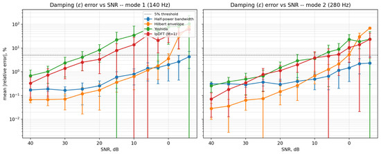
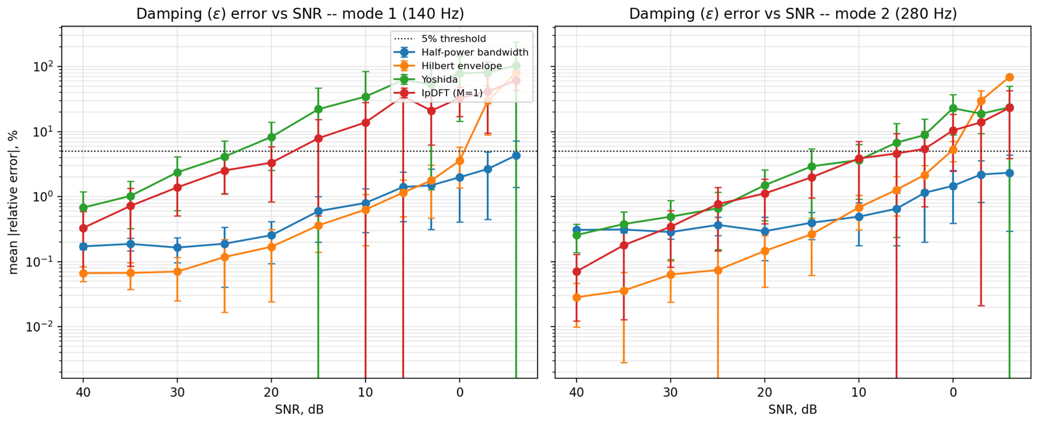
Figure 6 shows the mean relative error of εk as a function of SNR for each method individually. The four estimators exhibit markedly different noise sensitivity. Table 2 summarizes the SNR at which each method’s mean error exceeds 5% and 10%.
Figure 6.
SNR to error for mode 1 and mode 2 signal.
Table 2.
SNR at which the mean relative error in εk exceeds 5%/10%, for each estimator and mode.
The half-power bandwidth method, which draws on energy integrated across many spectral bins, remains within 5% error down to the lowest SNR tested. The Hilbert envelope method is accurate to approximately 0 dB SNR, but degrades abruptly below it, once the additive noise floor exceeds the decayed tail of the envelope and the underlying log-linearity assumption breaks down. The Yoshida and IpDFT methods, which rely on only three or four spectral bins adjacent to each spectral peak, are the most noise-sensitive, exceeding 5% error already at SNR values between roughly 5 and 25 dB depending on the mode.
An important practical consequence follows from this ranking: because the reported εk in Table 1 is an unweighted average of all four methods, its effective noise floor is set by the least robust contributing estimator (Yoshida/IpDFT) rather than by the most robust one (half-power bandwidth). At high SNR, characteristic of clean laboratory recordings, this averaging is unproblematic, as confirmed by the sub-percent errors in Table 1; at SNR below roughly 10–15 dB, however, the combined estimate should be expected to carry a materially larger error than the half-power method alone would, and this should be taken into account when interpreting damping values extracted from noisier or more distant-miked recordings.
The input overload observed in the Yamaha bass recording warrants discussion, since it is the one dataset in this study where the recorded waveform is measurably distorted rather than simply noisy. Clipping alters the shape of the waveform directly, flattening its peaks and introducing additional harmonic content that was not present in the original signal; this is qualitatively different from additive background noise, in that it represents a systematic, repeatable distortion of that specific recording rather than a random perturbation that would average out over repeated measurements. Because the reported damping coefficient is obtained by averaging four independent estimators—two of which (the half-power bandwidth and Hilbert-envelope methods) rely directly on the shape of the spectral peak and the amplitude envelope, both of which clipping can distort—the Yamaha εk estimates are more likely to carry a bias from this artifact than the Cort and Ibanez measurements, which were recorded without clipping. We therefore recommend that damping values derived from the affected Yamaha segments be interpreted with appropriate caution, particularly where direct cross-instrument comparisons of εk are drawn, and note this as a limitation of the present dataset rather than of the extraction algorithm itself.
3.2. Experimental Damping Profiles for Bass Guitars
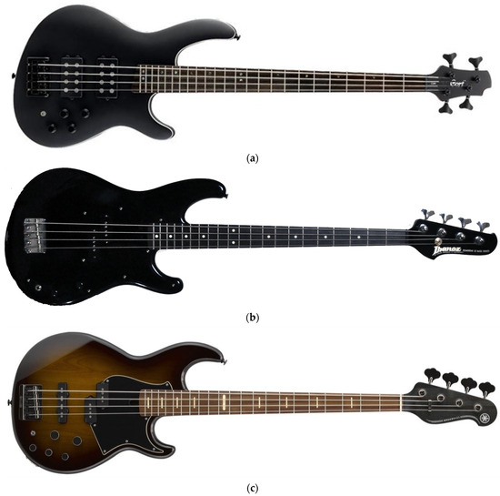
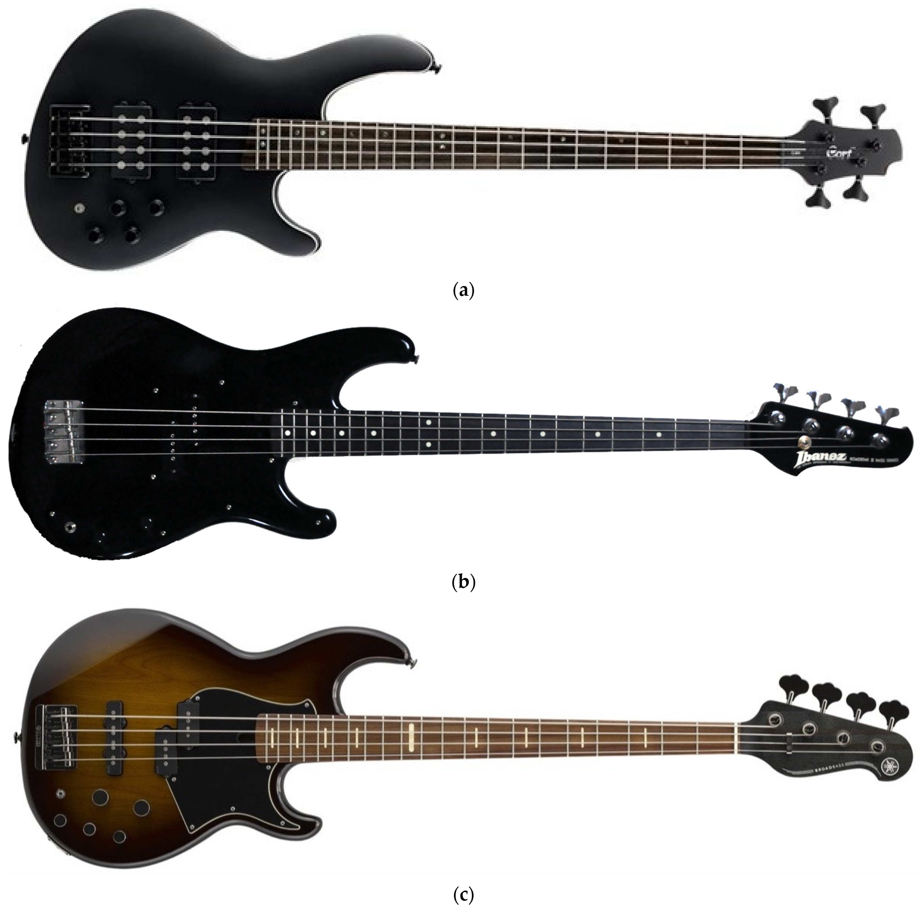
For the experimental determination of the damping parameters in the strings, electronic musical instruments are most convenient. There are no acoustic resonators in these instruments. To record their sound, simply connect them to the input of a computer audio interface. For this study, three bass guitars from different manufacturers were selected: Cort C4H, Ibanez RB 630, and a Yamaha bass (Figure 7). The damping parameters were determined when sound was excited on various frets and strings.
Figure 7.
Overview of the tested electric bass guitars used in the damping parameter identification experiments: (a) Cort C4H solid-body bass guitar; (b) Ibanez RB 630 Roadstar II series bass guitar; (c) Yamaha bass guitar (exact model unknown) [23].
The three instruments were deliberately chosen to span the two dominant electronic architectures found in mainstream solid-body bass guitars. The Ibanez RB 630 (Roadstar II series) is equipped with a single passive precision-style pickup and only passive volume/tone controls, representing the classical passive solid-body design that has served as the reference architecture for electric basses since the 1950s. The Cort C4H, in contrast, is fitted with active humbucking pickups and a switchable active two-band equalizer/preamp, representing the modern active solid-body architecture common on a large share of contemporary instruments. Both instruments share a conventional bolt-on neck, standard long scale length, and fretted fingerboard—i.e., the same basic mechanical boundary conditions assumed in the string vibration model of Section 2.1. The passive/active pairing of the Ibanez and Cort instruments is therefore intended to effectively cover the two mainstream electronic signal paths encountered in standard four-string, fixed-scale, fretted electric bass guitars, with the Yamaha recordings providing an additional, higher-quality third data point. The electronic differences between the two architectures (pickup type, presence or absence of an active preamp) are expected to primarily affect the recorded spectral envelope and noise floor rather than the underlying mechanical damping of the string itself, which is governed by the shared boundary and neck configuration described above.
For the first two bass guitars, sound was recorded through the line-in input of a personal-computer audio interface (44,100 Hz sample rate, 32-bit float, 23–25 dB SNR); the specific make and model of the audio interface were not documented at the time of the experiments and could not be reconstructed afterward, so only the resulting acquisition parameters are reported here. The third set of sounds was taken from the free sample library [23]. For each string–fret condition, a single clean take was recorded and retained for analysis; repeated takes of the same condition were not acquired, so run-to-run variability was not characterized at the acquisition stage.
Unlike the Cort and Ibanez recordings, whose acquisition chain (sample rate, bit depth, and SNR) is fully specified above, the Yamaha samples originate from a third-party, freely distributed library rather than from a recording session controlled by the authors. The source does not disclose the sample rate, bit depth, microphone or audio interface used, nor confirm the exact instrument model (Figure 7c), and these parameters could therefore not be matched to the Cort/Ibanez acquisition conditions. We include this dataset not as a matched third experimental condition, but as an independent test of the extraction algorithm’s generality on a recording whose provenance and equipment differ from, and are less controlled than, our own; absolute noise-floor or SNR comparisons across the three instruments should accordingly not be over-interpreted, and comparisons involving the Yamaha data are best read qualitatively.
The most general approximation of the damping parameter has been proposed in [3]:
where the coefficients d0–d3 are determined from the physical equations of various types of friction. However, the application of this model failed to achieve significant success. The results of the approximation of this model are given in Appendix A.
It is proposed to keep in (38) only a linear addendum. This means that the damping parameter εk depends on the frequency linearly:
The retention of only the linear term of the general damping model (38) is an engineering simplification rather than a claim that string damping is intrinsically linear in frequency. Physically, the modal damping of a plucked string arises from at least two mechanisms with distinct frequency signatures: air viscosity and support/termination losses, which are only weakly frequency-dependent, and internal (viscoelastic) friction in the string material, which grows with frequency [1,3]. Over the band of harmonics that carries most of the acoustic energy of a plucked bass note (roughly the first 10–12 partials), this composite dependence is smooth and monotonic, so a first-order truncation is a reasonable local approximation of the underlying physical law, analogous to a first-order expansion around the fundamental of the played note.
The high-order surface fitted in Appendix A (Table A1, Table A2 and Table A3) allows this assumption to be checked quantitatively rather than asserted. Comparing the fitted coefficients across the twelve string/instrument combinations shows that the linear term dominates (higher-order coefficients under ~20% of the linear term’s magnitude) for the Ibanez G-, A- and E-strings and the Cort E-string; for these cases the linear model (39) is close to exact. For the Ibanez D-string and the Yamaha G- and A-strings, higher-order coefficients are comparable to or larger than the linear term, indicating the linear model captures only the average trend and understates local curvature. Sound generated at higher frets or higher harmonics on these strings should be expected to show the largest deviation from the full model. For the Cort G-, D-, and A-strings and the Yamaha E-string, the fit assigns essentially no weight to the linear term at all, meaning the frequency dependence for these strings is dominated by curvature rather than a linear trend, and Equation (39) should be understood as a coarse average rather than a locally accurate fit in these cases. This pattern is not strongly separated by string identity alone, suggesting that instrument-specific construction (e.g., active vs. passive electronics, neck type) also contributes to the local shape of the damping curve, consistent with the discussion in Section 3.2.
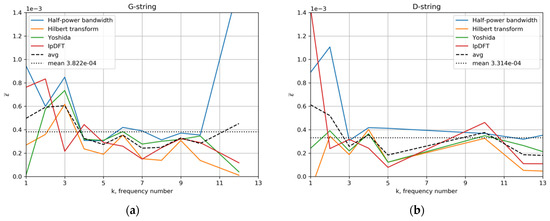
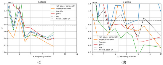
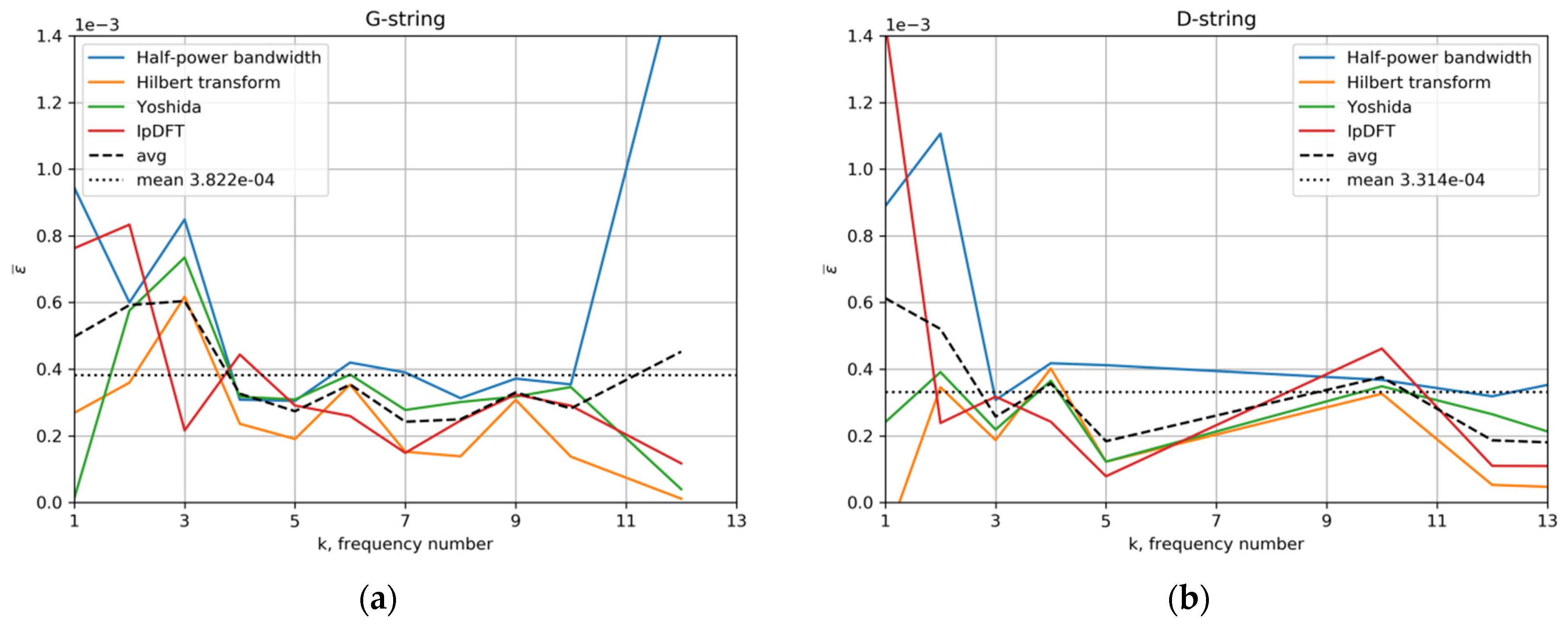
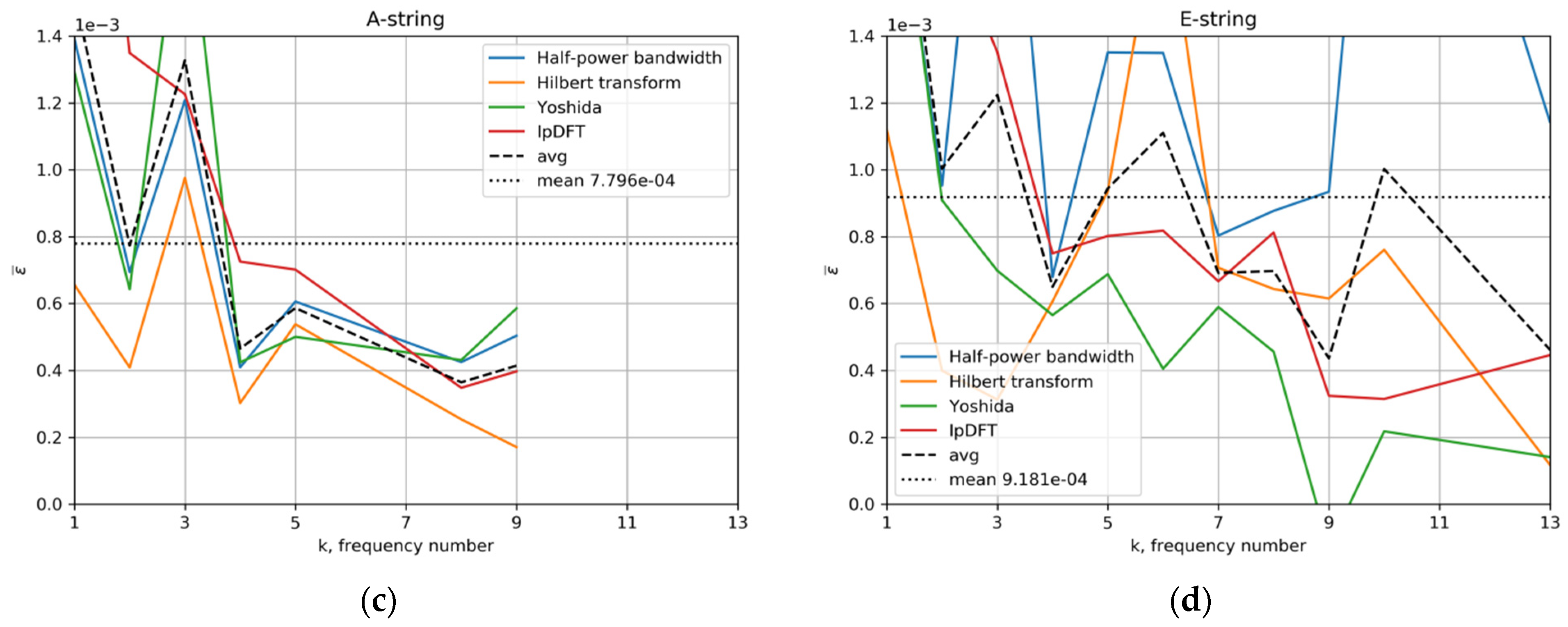
It means that for each guitar sound, only one parameter should be calculated. Figure 8 shows the dependence of the damping parameter on the frequency number k.
Figure 8.
Frequency-dependent behavior of the estimated damping parameter as a function of the harmonic frequency number k for the open strings of the Ibanez RB 630 bass guitar: (a) G-string; (b) D-string; (c) A-string; (d) E-string. The dashed black line represents the moving average (avg), and the dotted horizontal line denotes the calculated mean value for each respective string.
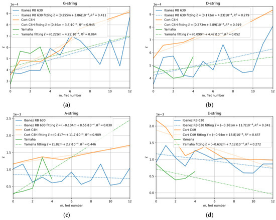
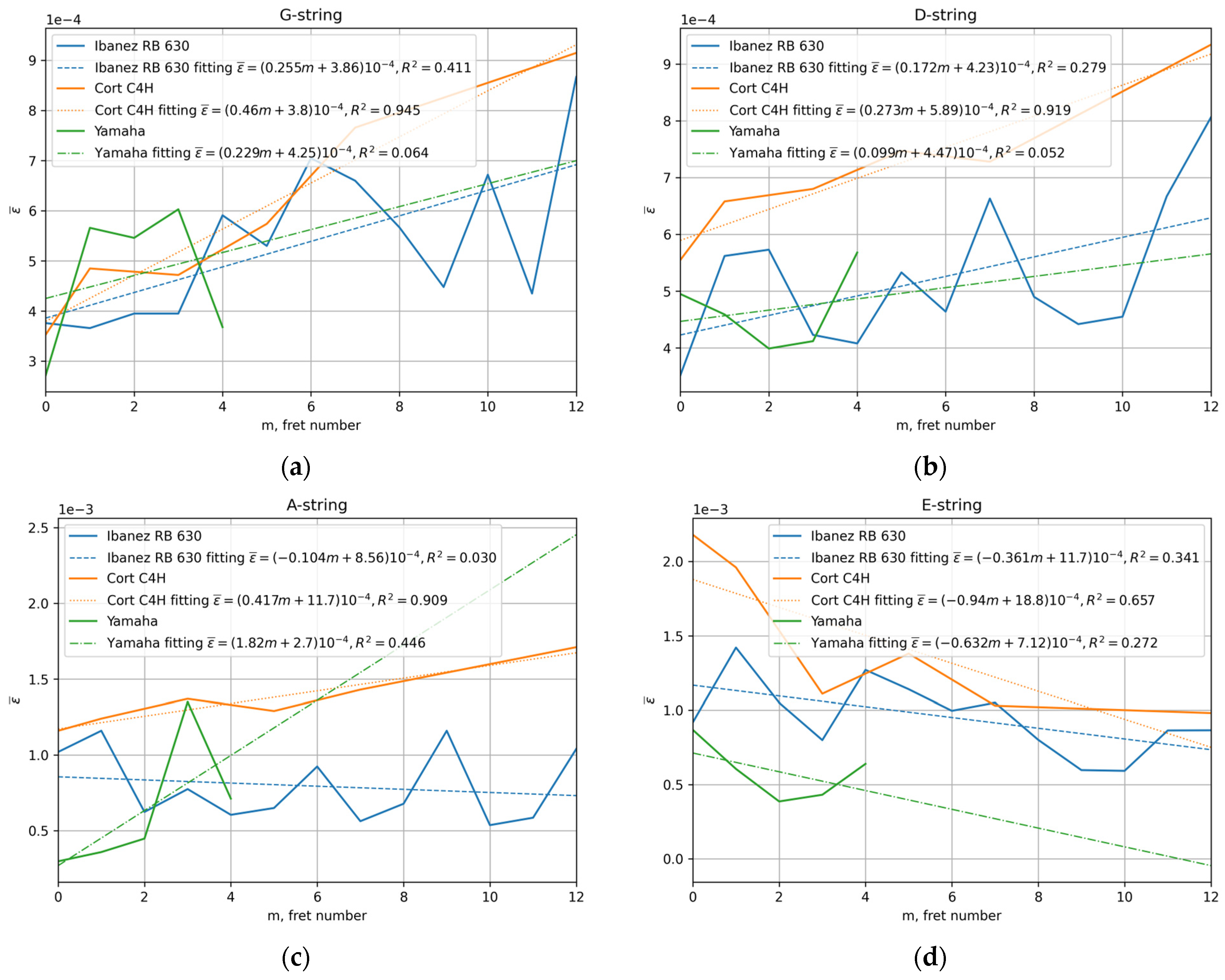
The next step is determining the dependence of the parameter on the number of the fret on which the sound is played. The results are shown in Figure 9, and the exact values are presented in Table 3, Table 4 and Table 5. As can be seen from the figures, the experimentally obtained dependences are quite complex; however, the general linear tendency is noticeable in them. Therefore, each figure shows the corresponding linear approximations of the data obtained. As can be seen from the figures for the strings of G and D for all three bass guitars, an increase in the parameter with an increase in the fret number is observed. For E-strings, an inverse effect is observed. The parameter decreases with increases in the fret number. The A-string is transitive; for Ibanez and Yamaha, the parameter increases, and for Cort C4H, the parameter decreases.
Figure 9.
Frequency-dependent behavior of the estimated damping parameter as a function of the fret number m of the Ibanez RB 630 bass guitar: (a) G-string; (b) D-string; (c) A-string; (d) E-string. Dashed lines show the corresponding linear approximations of the experimental data.
Table 3.
Estimated damping parameter for Ibanez RB 630.
Table 4.
Estimated damping parameter for Cort C4H.
Table 5.
Estimated damping parameter for Yamaha bass.
This pattern is consistent with known physical differences between bass guitar string gauges rather than being unexplainable. Moving from the G- to the E-string, standard bass string sets increase substantially in diameter and linear mass density ρ, typically by a factor of roughly 4–5 across a four-string set, while manufacturers generally aim to keep tension T comparable across strings within a set by adjusting core-to-winding proportions rather than diameter alone. Two consequences follow. First, thicker wound strings (A, E) contain proportionally more winding material and more winding-to-core contact area than the thinner G- and D-strings, and internal friction at these wire-to-wire contacts is an established source of damping in wound strings [1]; this is consistent with the systematically higher absolute εk values observed for the E-string relative to the G-string across all three instruments (Table 3, Table 4 and Table 5). Second, as the fret number increases, the vibrating length l shortens while the flexural rigidity of the string remains unchanged. Because the relative contribution of bending stiffness (and the associated inharmonicity and end-region losses at the nut/fret contact) grows as the vibrating length shrinks relative to the string’s diameter [1], thinner, nearly ideal strings (G, D)—for which this study’s flexible-string assumption (Section 2.1) holds most closely at open length—are more likely to show an increase in damping as this stiffness contribution becomes proportionally larger at higher frets. In contrast, thicker strings (E), in which internal/winding friction already dominates at open length, may show the opposite trend if shortening the string reduces the effective moment arm of that internal friction mechanism. The A-string, being intermediate in gauge, is the most likely to sit at the crossover between these two competing mechanisms, which would explain why its sign differs between instruments (Ibanez/Yamaha vs. Cort), depending on the specific string gauge and construction used on each instrument. We note that this explanation is qualitative: a fully quantitative confirmation would require the exact gauge, core/winding construction, and tension of the string sets used on each instrument, which were not recorded as part of this study and are noted here as a direction for future controlled testing.
It should be noted, however, that this coverage does not extend to instruments with substantially different mechanical boundary conditions. Multi-scale (fanned-fret) basses use a different effective vibrating length and string angle for each string, meaning that the single scale-length parameter l and the fixed pluck-position ratio l0/L used throughout this study would need to be re-derived independently per string rather than applied uniformly across the instrument. Headless basses, which anchor string tension and termination directly at the body/bridge assembly rather than through a separate neck-and-headstock structure, may exhibit different effective boundary stiffness at the nut/zero-fret end, which could alter the high-frequency damping behavior and shift the vibrating node structure discussed in Section 3.3 (e.g., the fifth harmonic node). Similarly, differences in neck construction (bolt-on vs. neck-through vs. set-neck) and neck material stiffness can change the effective mechanical impedance at the string termination points, which the present linear model treats as ideal rigid boundaries (Equations (2) and (3)). Applying the fret-dependent damping coefficients reported here to such instruments without re-calibration would therefore be expected to introduce systematic errors, particularly at higher frets and higher harmonics, where the assumption of ideal rigid boundary conditions is most likely to break down. Extending the identification framework to multi-scale and headless architectures, as well as explicitly incorporating boundary compliance into the vibration model, remains a subject for future work.
3.3. Sound Generation Strategies and Quality Assessment
To evaluate the practical applicability of the developed parameters, two distinct audio synthesis strategies are formulated and compared:
- Method 1 (spectrum-driven harmonic reconstruction). This strategy utilizes four distinct parameters extracted directly from the signal spectrum for each individual harmonic: the amplitude Ak, the frequency ωk, the phase φk, and the damping parameter εk. Thus, a total of 4N parameters is required to represent each synthesized sound, and the acoustic signal is reconstructed using the following superposition formula:
Because this approach relies purely on mathematical optimization of spectral components without physical boundary constraints, it can occasionally lead to combinations of parameters that are physically inconsistent.
- Method 2 (physics-based wave equation modeling). This approach is grounded strictly in the mechanical principles of string vibrations. Instead of independent parameters for each harmonic, the experimentally identified linear damping approximations (m) are injected directly into the continuous wave equation system (Equations (20)–(23)). This strategy requires the geometric constants of the instrument, specifically the scale length l = 0.8728 m and the bridge-to-pickup plucking location l0 = 0.185 m, which were obtained via direct physical measurements.
The proposed approach has several advantages. Utilizing a mathematical model allows for changing the timbre of the sound and the style of playing a musical instrument by changing the pickup point l0 and setting the initial speed. In principle, it can also represent other excitation techniques, such as slapping, through the non-zero initial-velocity condition of Equation (24). However, a full experimental validation of slap-type excitation against real slap recordings was outside the scope of this study.
To analyze the similarity between the original and generated bass guitar sounds, a robust quantitative measure is required. A normalized measure of similarity between two signals has been proposed in [24], which can be calculated:
where U1 and U2 are the Fourier spectra of signals. The value Q = 0 corresponds to the complete identity of the signals; the value Q = 1 means the absence of similarity.
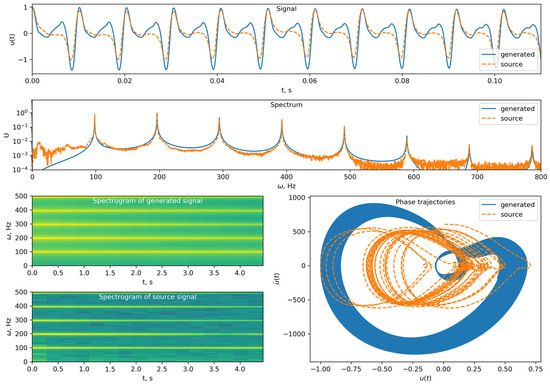
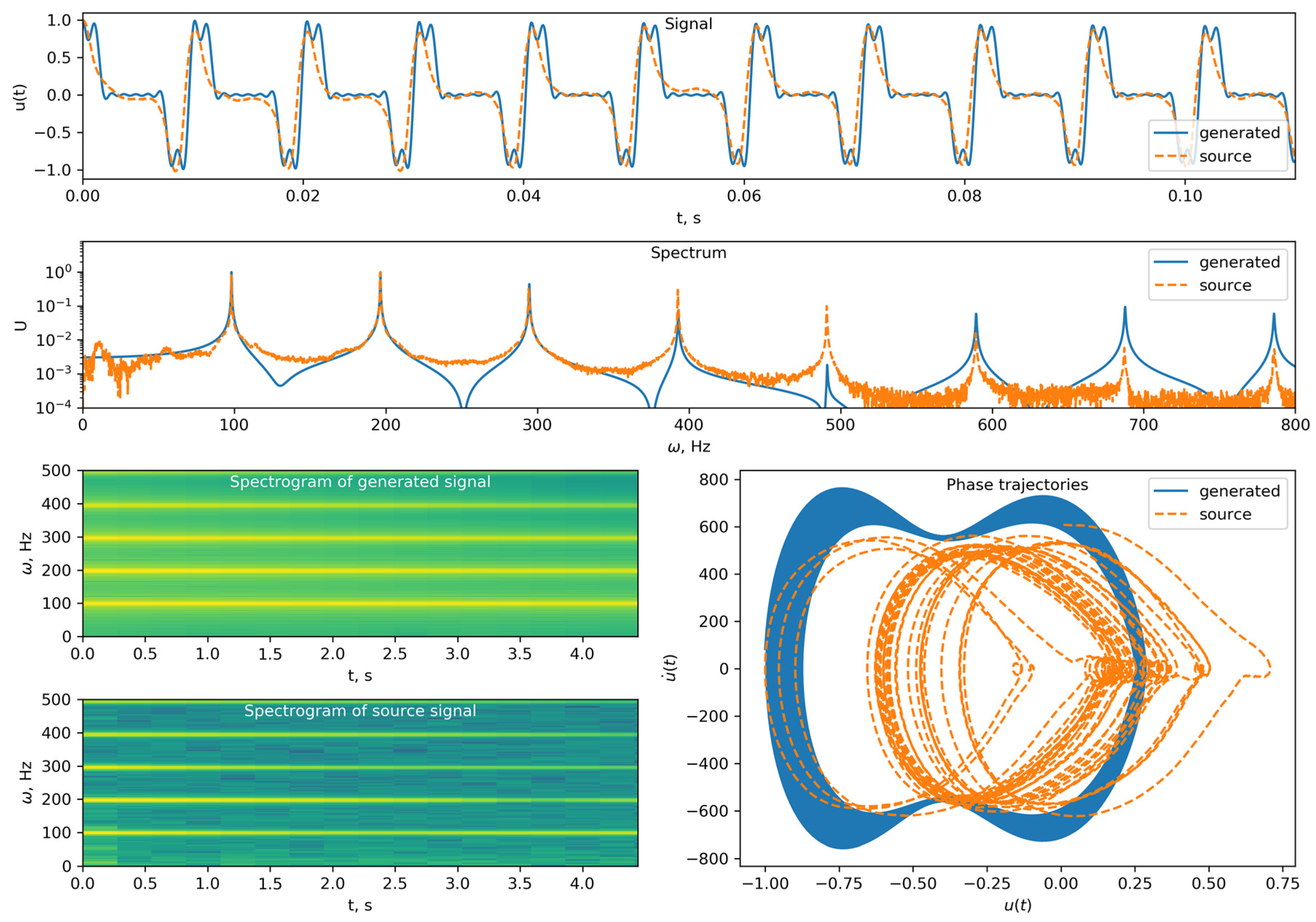
A comparison between the signal generated by Method 1 and the original open G-string signal of the Ibanez RB 630 bass guitar is presented in Figure 10. As can be seen from this graph, the signal spectra are in fairly good agreement, although noticeable discrepancies remain in the time-domain waveform shape and the resulting phase trajectories. Conversely, the comparison between the acoustic signal synthesized via Method 2 and the identical original open G-string recording is illustrated in Figure 11. According to the robust quantitative criterion based on the Sobolev norm of the signal differences, the calculated similarity measure yields Q = 0.057 for Method 1 and Q = 0.136 for Method 2. In this mathematical framework, the value of Q → 0 represents complete signal identity, while Q = 1 indicates a total lack of similarity. These structural error profiles mathematically confirm that while the spectrum-driven harmonic reconstruction (Method 1) achieves tighter spectral convergence, the physics-based wave equation approach (Method 2) ensures a significantly higher degree of physical fidelity regarding the continuous time-domain waveforms.
Figure 10.
Comparison of the signal generated by Method 1 with the original (Q = 0.057) Ibanez RB 630 open G-string.
Figure 11.
Comparison of the signal generated by Method 2 with the original (Q = 0.136) Ibanez RB 630 open G-string.
In the case of Method 2, the geometric shapes of the signals match the original reference much better, but a clear localized divergence is observed in the frequency domain. Specifically, a significant spectral difference occurs in the fifth harmonic region (~490 Hz). To provide a rigorous physical interpretation, given the direct geometric measurements of the instrument scale (l = 0.8728 m) and the fixed pluck zone (l0 = 0.185 m), the spatial excitation ratio evaluates to l0/L ≈ 0.212. This spatial coordinate sits in immediate proximity to the exact mathematical node of the fifth eigenmode (1/5 = 0.200). Consequently, the fifth harmonic falls into the nodal dead zone of the continuous wave field, meaning it is structurally suppressed during the mechanical excitation and pickup capture phases, which perfectly cross-validates the analytical behavior of the linear boundary framework.
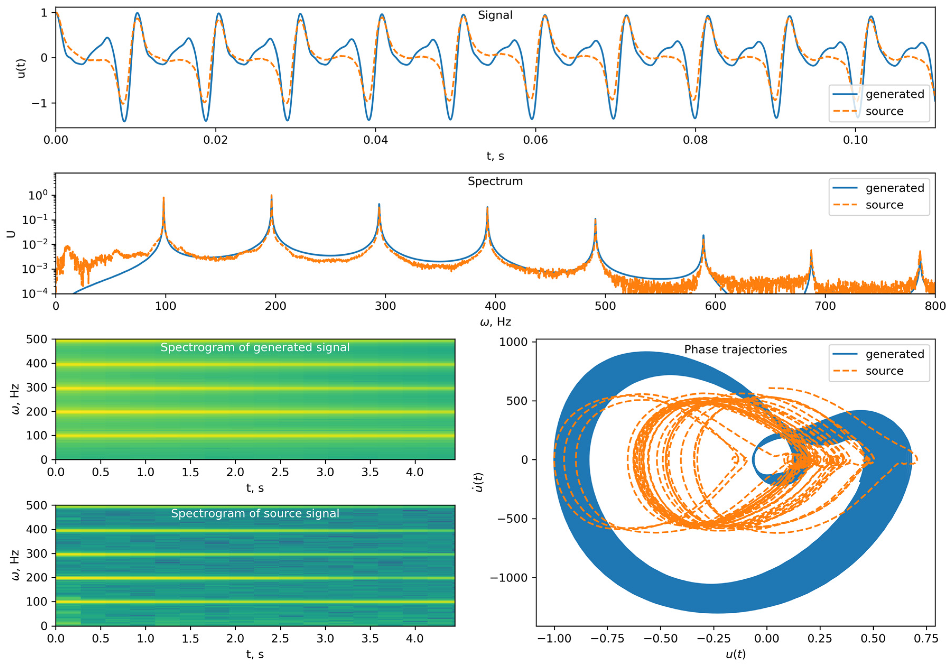
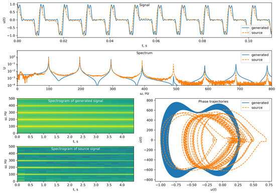
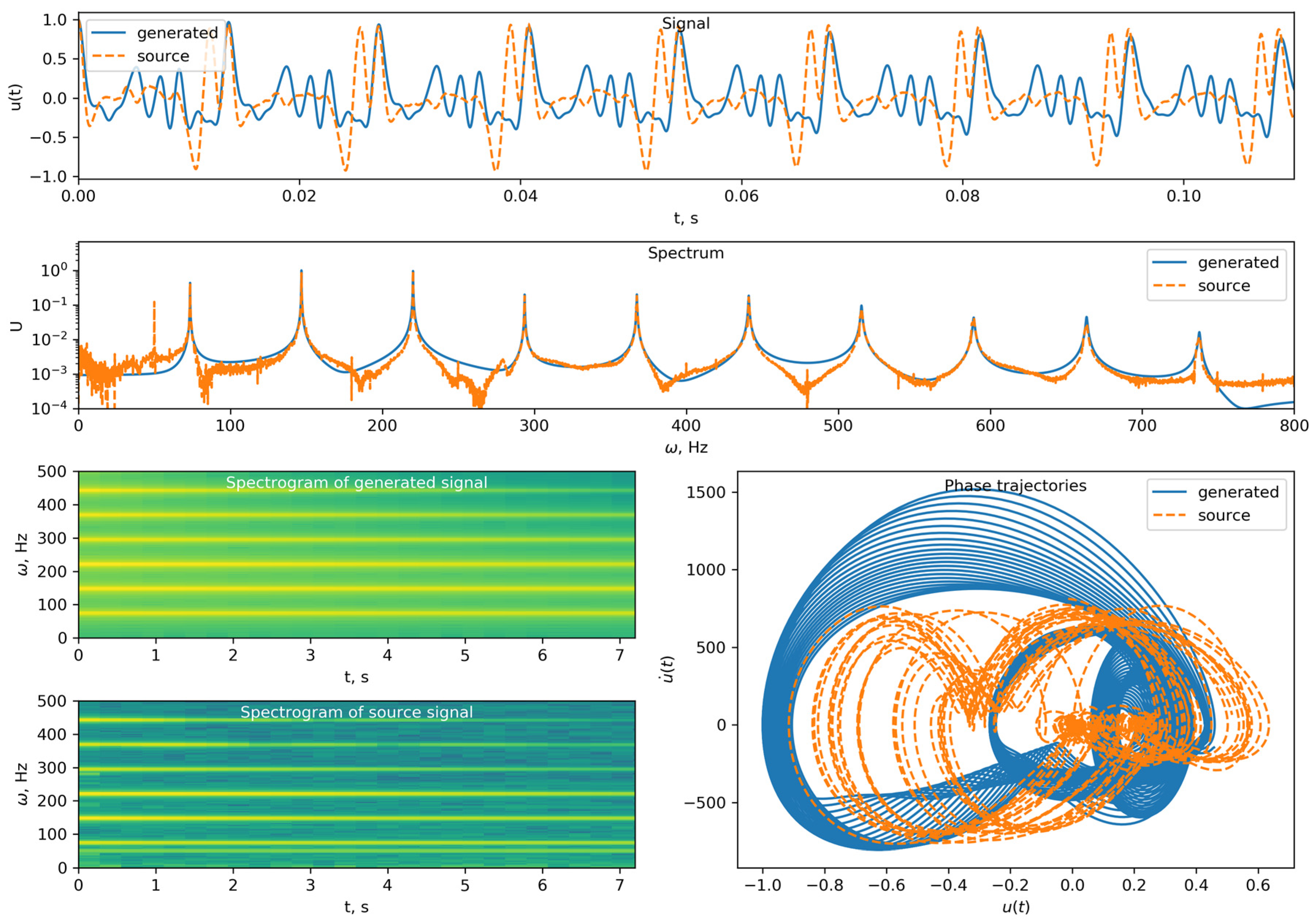
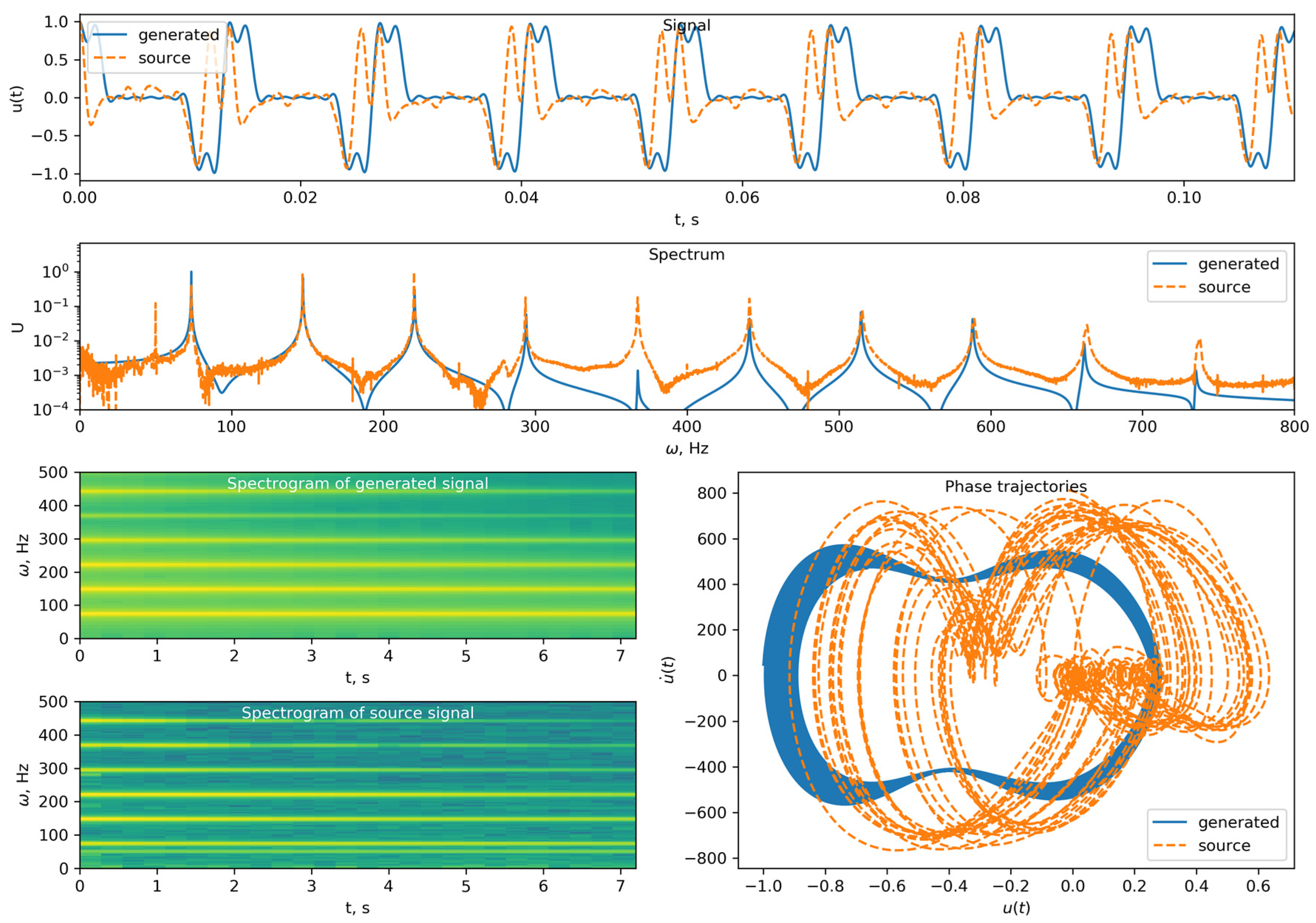
To analyze the quality of the obtained sounds, a comparison has been made between the generated and the original sound of the open string of the Cort C4H guitar. Despite the best correspondence in terms of the signal generated by Method 1 to the original one, there are significant differences in the form of the signal itself. Also worth noting is the phase trajectory obtained by this method. As shown in Figure 12 and Figure 13, the phase trajectory is quite complex, which is difficult to explain from a physical point of view. For the sound generated by Method 2, the phase trajectories correspond to the usual linear system. The shape of the signal in this case is much better consistent with the original one. This behavior underlines a critical limitation of non-physical optimization routines; without a governing structural equation, free harmonic parameter matching can result in phase-space loops that violate fundamental conservation laws. Conversely, the strict alignment of Method 2 with a formalized linear system guarantees structural stability and realistic energy decay envelopes, making it highly robust for practical physical modeling applications where playing style parameters vary dynamically. The frequency charts also deserve particular attention. It is clearly seen from these charts that the higher harmonics of the signal are damped much faster than the lower ones, and the attenuation process of these higher harmonics can be observed almost at the same time. This confirms the correctness of the constructed friction models.
Figure 12.
Comparison of the signal generated by Method 1 with the original (Q = 0.057) Cort C4H open D-string.
Figure 13.
Comparison of the signal generated by Method 2 with the original (Q = 0.153) Cort C4H open D-string. Colors on the spectrum shows signal amplitude.
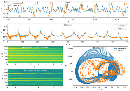
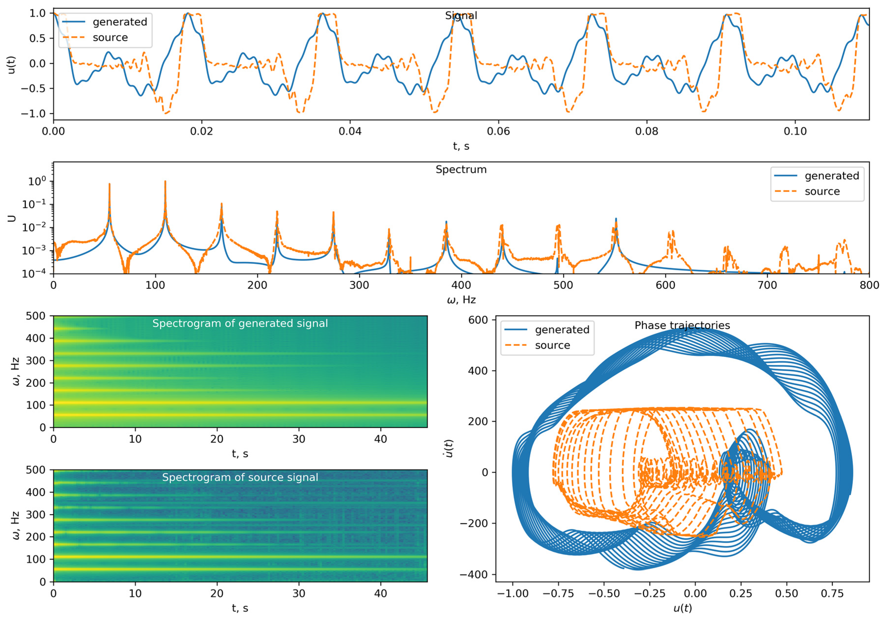
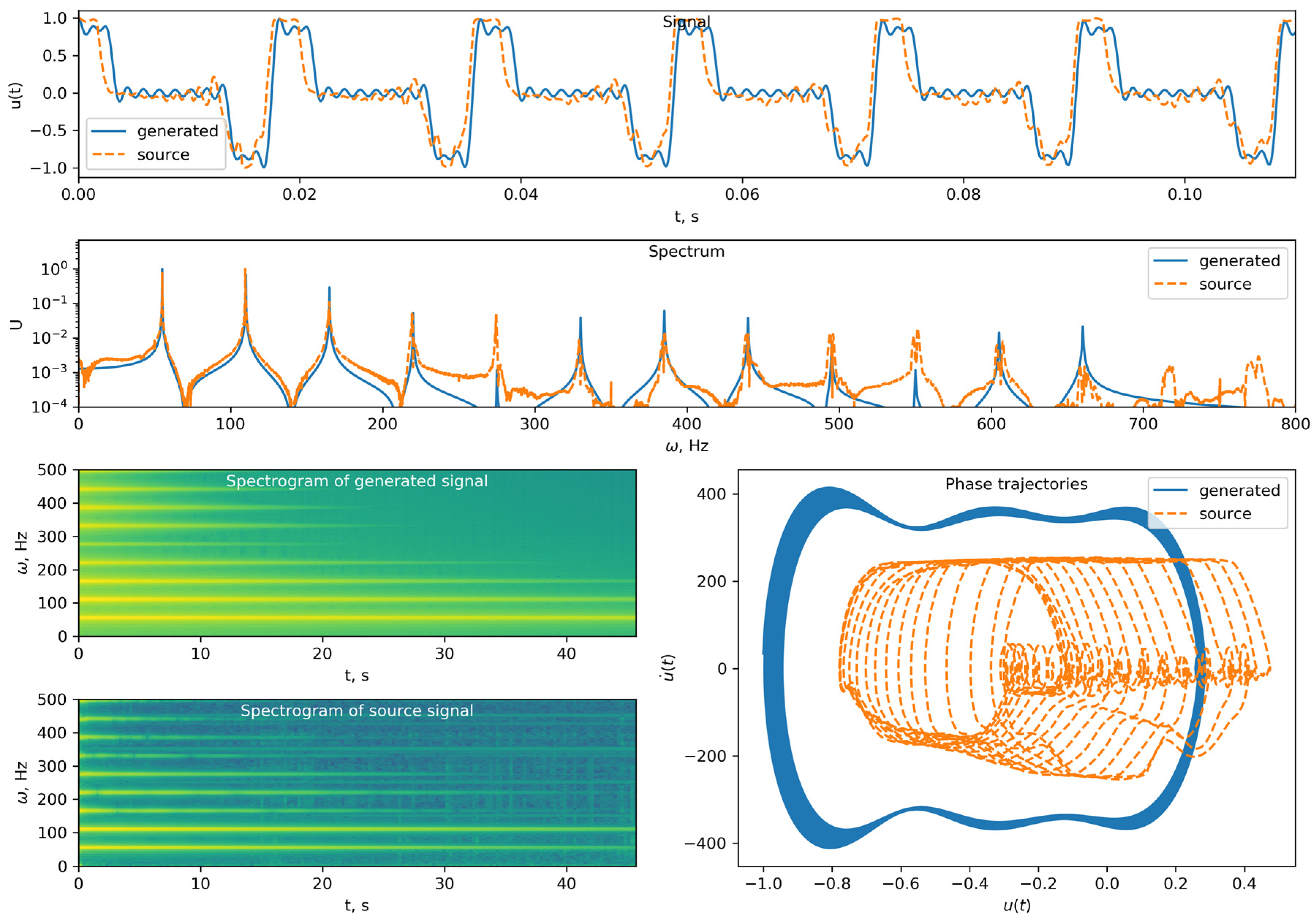
To ensure the comparison of results includes all three bass guitars, Figure 14 and Figure 15 show the comparison of sounds for the Yamaha bass guitar. From the signal spectra, it can be seen that these sounds are recorded on higher-quality equipment and have significantly less noise. However, as can be seen from the signal graphs, a deliberate or accidental error was made during their recording. In the first seconds of recording, the output of the guitar exceeded the allowable input level of the recording equipment. This led to the input channel being overloaded, and the signal was cut off from the top. On the phase trajectory, this phenomenon can also be observed in the form of a horizontal line. A distinctive feature of the samples for this guitar is the duration of the recording. The length of each recording is 40–50 s, which is 10 times longer than the other two. This made it possible to additionally analyze the damping rate of individual harmonics.
Figure 14.
Comparison of the signal generated by Method 1 with the original (Q = 0.031) Yamaha bass open A-string.
Figure 15.
Comparison of the signal generated by Method 2 with the original (Q = 0.058) Yamaha bass open A-string.
As can be seen from the time-frequency diagrams in Figure 14 and Figure 15, the first two harmonics have the lowest attenuation. It can also be seen that as the frequency increases, the harmonics in the original signal do not fade evenly. This situation better takes into account the first method of sound generation. In the case of the second method, in Figure 14, it can be seen that the imaginary line drawn through the end points of the sound is straight, with the sole exception of the fifth harmonic, which is poorly excited due to nodal constraints. The presence of such a line is a consequence of the use of the hypothesis that the damping parameter is linearly dependent on frequency.
Regarding the shape and spectrum of the signal, as with the previous two guitars, the first method gives better agreement on the spectrum, whereas the second method good in the form of a signal.
In addition to quantitative comparisons, qualitative expert assessments have been made. To carry out such studies, the original and generated signals were transmitted to experts who work with sound, asking them to determine which of the recordings are recorded sounds of a musical instrument and which are artificially synthesized. All experts agreed that all sounds are very similar and it is not possible to distinguish the generated signal from the real one. However, by ear, the signal generated by Method 1 has a slightly different timbre from the original signal and the signal generated by Method 2.
4. Conclusions
This study developed a linear string vibration model with experimentally identified, frequency- and fret-dependent modal damping, benchmarked four independent damping-estimation methods against synthetic and real recordings, and used the resulting parameters to drive two real-time bass guitar sound synthesis methods, validated against experimental recordings from three bass guitars (Ibanez RB 630, Cort C4H, and an externally sourced Yamaha dataset). The main findings are as follows.
Quantitative findings:
- Damping parameters can be estimated with sub-percent relative error under laboratory-grade conditions (23–25 dB SNR), but the least robust of the four estimators (Yoshida/IpDFT) exceeds 5% error once SNR falls below roughly 5–25 dB depending on the harmonic (Section 3.1).
- The damping parameter εk increases with fret number for the G- and D-strings across all three instruments, decreases for the E-strings, and is instrument-dependent for the A-string (increasing for Ibanez/Yamaha, decreasing for Cort C4H) (Section 3.2).
- Sobolev-norm comparison against ground-truth recordings gives Q = 0.031–0.057 for the spectrum-driven method (Method 1) and Q = 0.058–0.153 for the physics-based wave equation method (Method 2), indicating Method 1 achieves tighter spectral agreement while Method 2 better preserves time-domain waveform structure (Section 3.3).
- Method 1 requires 4N independently fitted, non-physical parameters (amplitude, frequency, phase, damping per harmonic) with no link to playing technique; Method 2 requires only physically grounded parameters (tension, density, pluck position/velocity, and the fitted εk damping surface), at the cost of the lower spectral accuracy above.
Limitations:
- The linear damping approximation (Equation (39)) closely matches the full high-order model (Appendix A) for only a subset of the tested strings; for others, the frequency dependence is dominated by curvature that the linear model cannot capture (Section 3.2), and highest-fidelity use cases should consult Appendix A directly.
- The Yamaha dataset originates from a third-party sample library with undocumented recording conditions and a clipping artifact; comparisons involving it should be read qualitatively rather than quantitatively (Section 3.2).
- For each string–fret condition, only a single valid recording was retained and analyzed; repeated takes were not recorded, so run-to-run variability arising from differences in plucking force, pluck position, and finger placement was not quantified. The reported damping values should therefore be read as single-trial estimates, and a formal repeatability (test–retest) analysis is left for future work.
- The model assumes a single fixed scale length and rigid boundary conditions and does not directly extend to multi-scale (fanned-fret) or headless bass designs without re-derivation (Section 3.2).
- The proposed physical explanation for string-dependent damping trends (string gauge and winding-friction effects) is a plausible hypothesis rather than one confirmed by direct gauge/tension measurement of the strings used.
- Real-time suitability is inferred from the closed-form, low-cost structure of both synthesis methods rather than measured directly: neither end-to-end latency nor per-note/per-voice computational time was benchmarked, and slap-type excitation, although representable through the non-zero initial-velocity condition (Equation (24)), was not experimentally validated. Quantitative real-time profiling and validation of slap articulation are identified as future work.
Practical implications:
- Both methods are closed-form and computationally lightweight relative to FDTD or full modal synthesis, making them suitable for real-time, multi-voice bass guitar synthesis (e.g., games, virtual instruments, education) without dedicated hardware acceleration, although absolute latency and per-voice computational cost were not benchmarked here (see Limitations).
- Method 1 is preferable where high spectral fidelity to a specific reference recording is the priority and playing-technique control is not required.
- Method 2 is preferable where dynamic control of playing technique (pluck position, velocity/slap articulation) is required, at a modest cost in spectral accuracy.
- All datasets and data processing Python 2.7 and 3.6 scripts are available on GitHub [27].
Author Contributions
Conceptualization, O.V.; methodology, O.V. and M.S.; software, O.V. and V.O.; validation, M.S., V.O. and O.A.; formal analysis, O.V. and M.S.; investigation, M.S. and V.O.; resources, O.V.; data curation, V.O. and O.A.; writing—original draft preparation, O.V. and M.S.; writing—review and editing, O.V. and O.A.; visualization, M.S. and V.O.; supervision, O.V.; project administration, O.V. All authors have read and agreed to the published version of the manuscript.
Funding
This research received no external funding.
Data Availability Statement
All data and code are available on github repository https://github.com/a-vodka/stingsoundgenerator, accessed on 27 July 2026.
Conflicts of Interest
The authors declare no conflict of interest.
Abbreviations
The following abbreviations are used in this manuscript:
| DFT | Discrete Fourier Transform |
| FFT | Fast Fourier Transform |
| IpDFT | Interpolated Discrete Fourier Transform |
| IpDTFT | Interpolation of Discrete-Time Fourier Transform |
| FDTD | Finite-Difference Time-Domain |
| GPU | Graphics Processing Unit |
Appendix A
To complement the simplified linear engineering framework discussed in the main text, this appendix presents the comprehensive structural identification results utilizing the high-order frequency-dependent damping model. While the main body of this study relies on localized linear approximations to preserve real-time synthesis efficiency, the continuous multi-parametric response surfaces capture complex mechanical interactions—such as internal molecular friction and boundary layer viscothermal losses—with higher mathematical precision.
The general non-linear polynomial approximation for the damping parameter surface is formulated as follows:
where m denotes the fret number, k represents the harmonic frequency number, and d0, …, d7 are the structural coefficients determined via multi-variable least squares optimization.
The exact numerical values of the optimized coefficients for each tested bass guitar architecture are detailed in Table A1, Table A2 and Table A3. Additionally, the corresponding continuous three-dimensional response surfaces mapped against experimental data points are illustrated in Figure A1, Figure A2 and Figure A3 to visualize the structural damping topologies. A quantitative comparison of the linear and high-order models—along with a discussion regarding which strings and playing ranges the linear simplification is least reliable for—is provided in Section 3.2.
Figure A1.
Reconstructed three-dimensional structural damping surfaces (ω, m) as a function of frequency ω and fret number m for the Ibanez RB 630 bass guitar: (a) G-string; (b) D-string; (c) A-string; (d) E-string. The continuous colored surfaces represent the high-order polynomial model approximations, while the red circular markers denote the experimentally identified damping parameters.
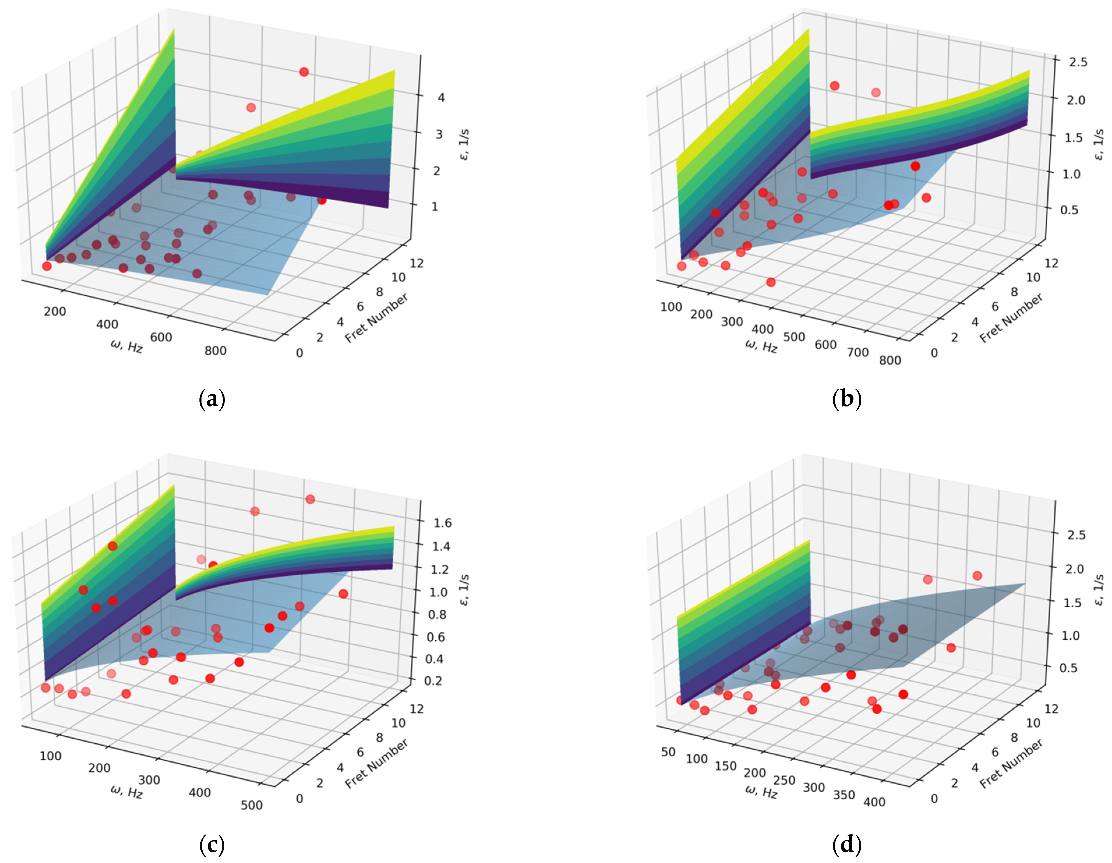
Table A1.
Damping approximation for Ibanez RB 630.
Figure A2.
Reconstructed three-dimensional structural damping surfaces (ω, m) as a function of frequency ω and fret number m for the Cort C4H bass guitar: (a) G-string; (b) D-string; (c) A-string; (d) E-string. The continuous colored surfaces represent the high-order polynomial model approximations, while the red circular markers denote the experimentally identified damping parameters.
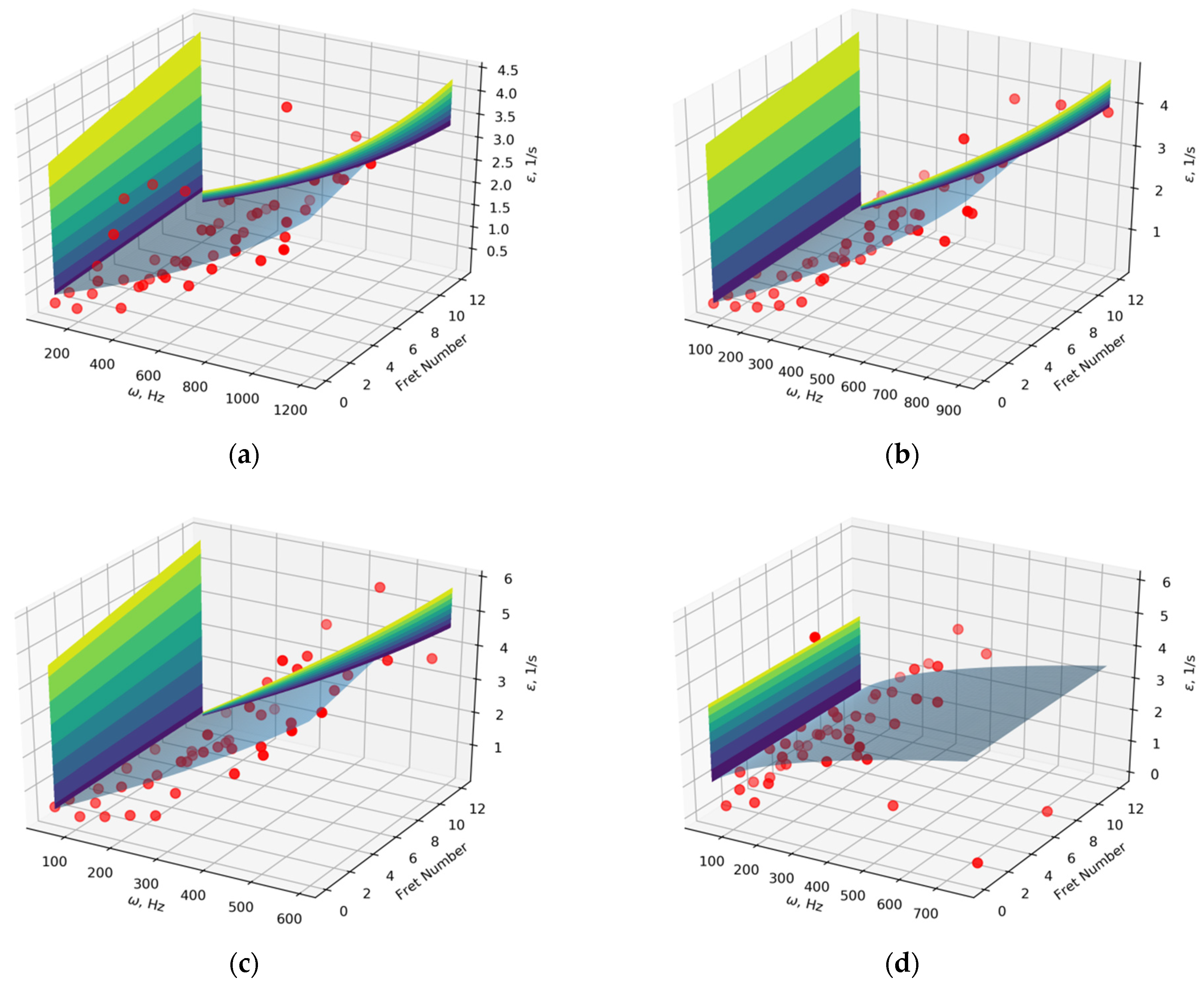
Table A2.
Damping approximation for Cort C4H.
Figure A3.
Reconstructed three-dimensional structural damping surfaces (ω, m) as a function of frequency ω and fret number m for the Yamaha bass guitar: (a) G-string; (b) D-string; (c) A-string; (d) E-string. The continuous colored surfaces represent the high-order polynomial model approximations, while the red circular markers denote the experimentally identified damping parameters.
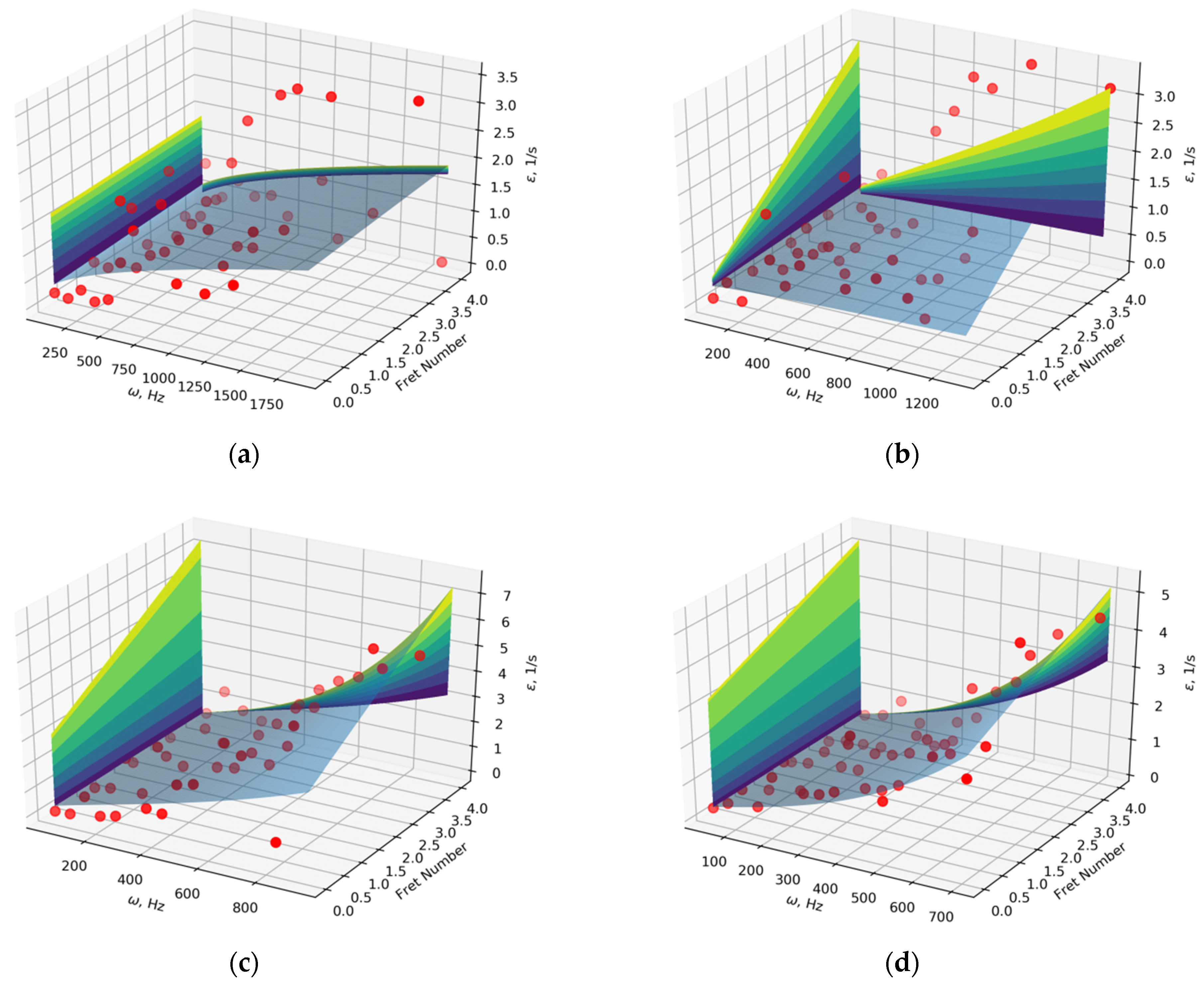
Table A3.
Damping approximation for Yamaha bass.
References
- Fletcher, N.H.; Rossing, T.D. The Physics of Musical Instruments; Springer: New York, NY, USA, 1998; pp. 97–130. [Google Scholar] [CrossRef] [Scilit]
- Vieira, M.; Infante, V.; Serrão, P.; Ribeiro, A.M.R. Experimental-numerical correlation of the dynamic behavior of the Portuguese guitar. Appl. Acoust. 2018, 131, 51–60. [Google Scholar] [CrossRef] [Scilit]
- Desvages, C.; Bilbao, S.; Ducceschi, M. Improved frequency-dependent damping for time domain modelling of linear string vibration. Proc. Meet. Acoust. 2016, 28, 035003. [Google Scholar] [CrossRef] [Scilit]
- Soares, F.; Cochelin, B.; Fréour, V.; Vergez, C.; Arimoto, K. Nonlinear acoustics in brass instruments using 2D complex modal bases. Acta Acust. 2025, 9, 49. [Google Scholar] [CrossRef] [Scilit]
- van Walstijn, M.; Chatziioannou, V.; Bhanuprakash, A. Implicit and explicit schemes for energy-stable simulation of string vibrations with collisions: Refinement, analysis, and comparison. J. Sound Vib. 2024, 569, 117968. [Google Scholar] [CrossRef] [Scilit]
- Woodhouse, J.; Politzer, D.; Mansour, H. Acoustics of the banjo: Measurements and sound synthesis. Acta Acust. 2021, 5, 15. [Google Scholar] [CrossRef] [Scilit]
- Belega, D.; Petri, D. Fast interpolated DTFT estimators of frequency and damping factor of real-valued damped sinusoids. Measurement 2023, 217, 113076. [Google Scholar] [CrossRef] [Scilit]
- Das, I.; Arif, M.T.; Than Oo, A.M.; Subhani, M. An Improved Hilbert–Huang Transform for Vibration-Based Damage Detection of Utility Timber Poles. Appl. Sci. 2021, 11, 2974. [Google Scholar] [CrossRef] [Scilit]
- Enache, R.G.; Nica, G.B.; Ionică, G.; Vînătoru, I.A. Parametric Study of Damping Ratio Estimation Using Ambiental Vibration Recordings. Sustainability 2026, 18, 2645. [Google Scholar] [CrossRef] [Scilit]
- Lee, J.W.; Park, J.; Choi, M.J.; Lee, K. Differentiable Modal Synthesis for Physical Modeling of Planar String Sound and Motion Simulation. arXiv 2024, arXiv:2407.05516. [Google Scholar] [CrossRef] [Scilit]
- Comunità, M.; Stowell, D.; Reiss, J. Guitar Effects Recognition and Parameter Estimation with Convolutional Neural Networks. J. Audio Eng. Soc. 2021, 69, 594–604. [Google Scholar] [CrossRef] [Scilit]
- Das, O.; Abel, J.S. Modal Estimation on a Warped Frequency Axis for Linear System Modeling. arXiv 2022, arXiv:2202.11192. [Google Scholar] [CrossRef] [Scilit]
- Yu, Y.; Qin, X.; Hussain, S.; Hou, W.; Weis, T. Pedestrian Counting Based on Piezoelectric Vibration Sensor. Appl. Sci. 2022, 12, 1920. [Google Scholar] [CrossRef] [Scilit]
- Smith, J.O. Principles of Digital Waveguide Models of Musical Instruments. In Applications of Digital Signal Processing to Audio and Acoustics; Kahrs, M., Brandenburg, K., Eds.; The International Series in Engineering and Computer Science; Springer: Boston, MA, USA, 2002; Volume 437. [Google Scholar] [CrossRef] [Scilit] [PubMed]
- Anaya, S.G.; Moura, H.G.; Teodoro, E.B.; de Miranda, R.F.; Muñoz, D.M. A comprehensive digital waveguide formulation using the impedance method for acoustic simulation. Mech. Syst. Signal Process. 2025, 224, 112047. [Google Scholar] [CrossRef] [Scilit]
- Tablas de Paula, P.; Smith, J.O., III; Välimäki, V.; Reiss, J.D. Four Decades of Digital Waveguides. arXiv 2026, arXiv:2604.12878. [Google Scholar] [CrossRef] [Scilit]
- Bilbao, S.; Russo, R.; Webb, C.J.; Ducceschi, M. Real-time guitar synthesis. In Proceedings of the 27th International Conference on Digital Audio Effects (DAFx24), Surrey, UK, 3–7 September 2024; pp. 163–170. [Google Scholar]
- Russo, R.; Webb, C.J.; Ducceschi, M.; Bilbao, S. Convergence analysis and relaxation techniques for modal scalar auxiliary variable methods applied to nonlinear transverse string vibration. Proc. Meet. Acoust. 2025, 56, 035007. [Google Scholar] [CrossRef] [Scilit]
- Zieliński, T.; Duda, K. Frequency and Damping Estimation Methods—An Overview. Metrol. Meas. Syst. 2011, 18, 505–528. [Google Scholar] [CrossRef] [Scilit]
- Papagiannopoulos, G.A.; Hatzigeorgiou, G.D. On the use of the half-power bandwidth method to estimate damping in building structures. Soil Dyn. Earthq. Eng. 2011, 31, 1075–1079. [Google Scholar] [CrossRef] [Scilit]
- Yoshida, I.; Sugai, T.; Tani, S.; Motegi, M.; Minamida, K.; Hayakawa, H. Automation of internal friction measurement apparatus of inverted torsion pendulum type. J. Phys. E Sci. Instrum. 1981, 14, 1201–1206. [Google Scholar] [CrossRef] [Scilit]
- Duda, K.; Magalas, L.B.; Majewski, M.; Zielinski, T.P. DFT-based Estimation of Damped Oscillation Parameters in Low-Frequency Mechanical Spectroscopy. IEEE Trans. Instrum. Meas. 2011, 60, 3608–3618. [Google Scholar] [CrossRef] [Scilit]
- Free Yamaha Bass Guitar Sample Library. Available online: http://kontaktlibraries.com/free-yamaha-bass-guitar-kontakt-library/ (accessed on 6 June 2026).
- Perlin, M.; Bustamante, M.D. A robust quantitative comparison criterion of two signals based on the Sobolev norm of their difference. J. Eng. Math. 2016, 101, 115–124. [Google Scholar] [CrossRef] [Scilit]
- Paté, A.; Le Carrou, J.-L.; Fabre, B. Predicting the decay time of solid body electric guitar tones. J. Acoust. Soc. Am. 2014, 135, 3045–3055. [Google Scholar] [CrossRef] [Scilit] [PubMed]
- Dignam, C. Harmonies on the String: Exploring the Synergy of Music and STEM. Int. J. Technol. Educ. Sci. 2024, 8, 491–521. [Google Scholar] [CrossRef] [Scilit]
- Vodka, O. Bass Guitar Sound Dataset and Data Processing Scripts. 2018. Available online: https://github.com/a-vodka/stingsoundgenerator (accessed on 6 June 2026).

Disclaimer/Publisher’s Note: The statements, opinions and data contained in all publications are solely those of the individual author(s) and contributor(s) and not of MDPI and/or the editor(s). MDPI and/or the editor(s) disclaim responsibility for any injury to people or property resulting from any ideas, methods, instructions or products referred to in the content. |
© 2026 by the authors. Licensee MDPI, Basel, Switzerland. This article is an open access article distributed under the terms and conditions of the Creative Commons Attribution (CC BY) license.