


Highlights
What are the main findings?
- Five quadrotor SDR path-loss datasets (433–3300 MHz; overwater, suburban, and mountainous) on which PACE-A2G matches strong tree ensembles and yields 90% prediction intervals with 0.88–0.97 coverage.
- Random splits overstate accuracy on single-flight data: chronological-split RMSE is 1.9 to 8 times the random-split value, and all learned models degrade sharply under cross-scenario transfer.
What are the implications of the main findings?
- Benchmarks for learned air-to-ground channel models should report chronological and spatial splits alongside random splits.
- Conformal calibration does not survive domain shift, but a feature-space detector flags every shifted source–target pair, and a few labelled records of the new domain restore near-nominal coverage.
Abstract
Air-to-ground (A2G) channel modeling supports low-altitude wireless networks for unmanned aerial vehicle (UAV) services in 5G/6G systems. Existing data-driven models are often benchmarked against weak empirical baselines, decoupled from the underlying measurement campaigns, and prone to overfitting on small UAV datasets. This paper presents PACE-A2G, a calibrated deep-tree ensemble on physics-aware features, together with a stricter evaluation methodology. A quadrotor-mounted software-defined-radio measurement system produces five datasets covering 433, 740, 1500, and 3300 MHz in overwater, suburban, and mountainous environments. The deep tabular backbone combines periodic numerical embeddings, feature-group attention, and a parameter-efficient ensembling head; propagation physics enters through the features rather than through the architecture. At inference, the deep estimate is blended with a tree ensemble, and a split-conformal quantile head provides calibrated prediction intervals. Evaluation under random, chronological, and spatial-block protocols shows that random partitions overestimate accuracy: the chronological-split root-mean-square error (RMSE) of the strongest tree-ensemble baseline is 1.9 to 8 times its random-split value. In distribution, the hybrid predictor is statistically on par with the strongest tree ensembles. Across nine cross-scenario and cross-frequency protocols, it transfers more robustly than the tree ensemble on balance, with a mean paired RMSE reduction of 0.34 dB, although the fitted log-distance baseline remains the strongest single predictor under shift. Split-conformal calibration reaches near-nominal 90% coverage in distribution but collapses under domain shift; a feature-space out-of-distribution gate detects the shift on every source–target pair, and ten labelled records of the new domain restore near-nominal coverage.
1. Introduction
As unmanned aerial vehicle (UAV) technology advances and 5G and 6G networks evolve, A2G links have become a core part of low-altitude wireless networks (LAWNs) [1]. Accurate A2G channel models support system design, spectrum allocation, interference coordination, and network optimization [2]. These links are difficult to model because they involve distinctive 3-D propagation, strong time variation, and complex multipath caused by low-altitude reflection and scattering [3].
Existing model-based, measurement-driven, and learning-based approaches, reviewed in Section 2, leave three needs unmet: benchmarks that at least partially decouple carrier frequency from the scenario, evaluation protocols that respect the spatio-temporal structure of flight data, and calibrated predictive uncertainty for deployment. This paper proposes PACE-A2G, a calibrated ensemble framework for A2G channel modeling that combines physics-informed feature design with data-driven learning. The main contributions are summarized as follows:
- A software-defined-radio (SDR)-based quadrotor measurement campaign yields five datasets grouped by frequency and scenario, containing 4213 calibrated path-loss points at 433, 740, 1500, and 3300 MHz in overwater, suburban, and mountainous environments. The campaign partially decouples carrier frequency from scenario: 433 MHz is measured in both the overwater and the suburban environment, whereas 740 MHz is measured only over water and 1500 and 3300 MHz only in the mountains.
- A 14-D geometric and electromagnetic feature vector is fed through a periodic numerical embedding, a feature-group attention encoder, and a parameter-efficient ensembling regression head. The propagation physics enters through this feature design; the network itself is a generic tabular architecture. The deployed hybrid blends this deep backbone with a random forest and is statistically on par with the strongest tree ensembles under in-distribution random splits. Across nine cross-scenario and cross-frequency transfer protocols, it attains lower RMSE than the tree ensemble on four protocols, statistically comparable RMSE on three, and higher RMSE on two, with a mean paired improvement of 0.34 dB. The fitted log-distance baseline remains the strongest single predictor under shift.
- Random, chronological, and spatial-block protocols are reported side by side across the five datasets and a fourteen-model comparison suite. For the strongest tree-ensemble baseline, the chronological-split root-mean-square error (RMSE) is 1.9 to 8 times higher than the random-split RMSE, showing that random partitions overestimate accuracy on single-flight A2G data and motivating the stricter benchmarks used throughout.
- A conformalized quantile head delivers 90%-nominal prediction intervals with empirical coverage between 0.88 and 0.97 in distribution and a finite-sample guarantee. This coverage collapses under domain shift; a feature-space out-of-distribution gate, evaluated on all 20 source–target pairs, detects every shifted pair, and recalibration from ten labelled records of the new domain restores coverage of 0.85 to 0.96.
2. Related Work
2.1. Model-Based and Empirical A2G Channel Modeling
Existing A2G channel modeling mainly uses deterministic site-specific solvers or closed-form statistical models [3]. Deterministic methods solve Maxwell’s equations or trace rays through a three-dimensional environment model. Commercial ray-tracing engines and direct numerical solvers such as FDTD can give reference-quality field predictions when terrain and material parameters are accurate. Their cost grows steeply with simulation volume and with the number of frequency points, which makes a full sweep over the pitch, azimuth, and altitude envelope of a low-altitude UAV trial impractical in a single calibration. Statistical and empirical models are simpler but less faithful to the propagation environment. Okumura–Hata [4] and the COST-231 Hata extension [5] use linear log-distance terms with categorical environment corrections fitted on ground-to-ground cellular links. The 3GPP TR 38.901 UMa-AV [6] and TR 36.777 [7] aerial vehicle extensions provide cellular-UAV path-loss formulas calibrated above 1 GHz on urban-macro deployments. Across both model classes, fixed-form expressions generalize poorly across scenarios [3,8]. They also struggle to capture the nonlinear coupling among link distance, pitch angle, Fresnel-zone clearance, and scenario class that drives LAWN A2G shadowing.
2.2. UAV A2G Measurement Campaigns
Reliable channel models require measurement campaigns that cover the operating envelope. Early manned-aircraft campaigns at C and L bands swept overwater, hilly, and near-urban terrain [9,10,11,12]. They established a methodological baseline that is still used, but the cost of each flight limited parameter coverage. UAV platforms have since become flexible and lower-cost alternatives [13,14]. Reported campaigns now cover urban canyons [15], suburban streets [16], and campus environments [17,18]. High-quality LAWN A2G datasets that span multiple bands and scenarios are still scarce because of payload and endurance limits [18,19], terrain-restricted maneuverability [20], and the difficulty of obtaining multi-band sounding under one calibration [21,22]. Measurement-based characterization efforts have produced calibrated overwater path-loss traces at sub-1.5 GHz carriers [23]. The present work contributes a five-dataset benchmark spanning overwater, suburban, and mountainous environments at four carriers, used throughout the paper.
2.3. Learning-Based Channel Modeling and Data Augmentation
Deep learning can learn nonlinear mappings under multidimensional parameter coupling and has shown strong potential for channel modeling [24,25,26]. Most published deep channel models still rely on training sets of – samples, which single-flight LAWN campaigns cannot provide. A domain-specific framework that aligns the learning objective with propagation physics is also still missing [22]. In the small-sample regime, meta-learning across related tasks can regularize the predictor [27], but a per-campaign LAWN setting offers few related source tasks. Data augmentation enlarges the effective training set. Generative augmentation with generative adversarial networks or variational autoencoders [28] can produce additional samples at low cost, yet it is not aware of propagation physics and may violate the free-space lower bound. Mixup-style interpolation [29] is more conservative because synthetic samples are convex combinations of real ones. The remaining issue is how to constrain the pairing rule so that interpolated samples stay on the physical manifold instead of crossing scenario or frequency boundaries.
2.4. Attention Mechanisms and Research Gap
Attention mechanisms, especially multi-head attention (MHA) [30], model long-range dependencies among input tokens and have been used in speech, vision, and physical-layer wireless tasks [31,32]. In LAWN A2G modeling, deep predictors usually fuse heterogeneous geometric and electromagnetic quantities through one embedder. They are rarely compared with the gradient-boosted and bagged tree ensembles that dominate small-sample tabular regression [33]. Their behavior under realistic distribution shift and their predictive uncertainty are also seldom reported. The framework proposed here treats these issues as central. It injects propagation priors through a 14-D physics-aware feature design, feeds those features into a tabular network whose attention is organized by feature group, and benchmarks the predictor against strong tree-ensemble and closed-form empirical baselines under random, chronological, and spatial-block protocols. It further evaluates cross-scenario and cross-frequency transfer directly and equips the model with split-conformal calibrated prediction intervals.
3. Materials and Methods
Figure 1 overviews the PACE-A2G pipeline, from SDR measurement acquisition through physics-aware feature engineering to the deep tabular backbone, the tree blend, and split-conformal calibration. This section details each stage.
Figure 1.
End-to-end LAWN A2G channel-modeling pipeline of PACE-A2G. Stage 1 ingests the raw SDR sounding records of the five measurement sets grouped by frequency and scenario. Stage 2 derives the 14-D physics-aware feature vector. Stage 3 applies the deep tabular backbone, detailed in Section 3.5. Stage 4 blends the deep estimate with a random forest and applies a split-conformal quantile head; the feature-space out-of-distribution gate of Section 3.6, which decides at deployment whether the in-distribution interval may be used, acts inside this stage and is not drawn separately. The output is the path-loss point estimate in dB and a near-nominal 90% prediction interval for the measured path loss . Training uses a Smooth-L1 plus pinball objective.
3.1. Design of the LAWN A2G Channel Measurement System
We design a modular SDR-based LAWN A2G measurement system with a distributed airborne transmitter (TX) and ground receiver (RX). The UAV is a professional-grade quadrotor with centimeter-level real-time kinematic (RTK) positioning and 20 min of endurance under a 2 kg payload. The airborne TX uses a USRP E312 to generate PN9 pseudo-random signals. An external power amplifier (PA) amplifies the signal, and an onboard omnidirectional antenna radiates it. The ground RX uses a USRP B210 with a low-noise-amplifier (LNA) front end, and samples are streamed over USB 3.0 to the host computer for real-time processing and storage. Both the TX and RX use GNU Radio 3.10. Both terminals carry GPS modules that output 1-PPS signals for TX and RX clock synchronization. The measurement methodology follows established SDR-based UAV channel-sounding practice [23]. The campaigns cover four carrier frequencies with an explicit frequency–scenario mapping: 433 MHz in the overwater and suburban scenarios, 740 MHz in the overwater scenario, and 1500 and 3300 MHz in the mountainous scenario. TX power is set to 30 dBm for line-of-sight (LoS) coverage over the planned range. RTK positioning provides centimeter-accurate transceiver coordinates for 3-D link-geometry computation. For every sounding record, the measured path loss is in dB, where is the logged transmit power and the received power measured by the ground RX; this quantity is the regression target y used throughout the paper.
3.2. Measurement Campaign and Datasets
Three scenario types are covered, as shown in Figure 2: overwater, suburban, and mountainous. The hilly–mountainous site has 200 to 450 m elevation variation, mixed vegetation, and rocky scatterers. The overwater site offers a ∼1 km2 water surface bounded by sparse low-rise structures; the suburban site lies in the same region and features similar low-rise development. Each campaign combines manual piloting and autonomous navigation, with flight altitudes of 0 to 50 m and horizontal distances of 0 to 350 m. A flight pattern of circular orbits and linear passes provides pitch coverage from 10° to 85°. Each point is sampled for 1 s at 2 MHz. RTK records UAV position and attitude, while the ground RX synchronously records I/Q and received power. The full campaign yields 4213 measurement points across five frequency–scenario datasets, denoted W433, S433, W740, M1500, and M3300, where W, S, and M indicate the overwater, suburban, and mountainous scenarios and the number gives the carrier frequency in MHz. Table 1 lists, for each dataset, the number of sounding records, the number retained after the interquartile-range (IQR) outlier rule of Section 4.1, the fences, and the ranges of retained path loss and 3-D link distance. Each dataset is a single continuous flight, and the five flights differ in scenario, in carrier, or in both.
Figure 2.
Measurement scenarios and multi-frequency channel overview for the five LAWN A2G datasets used throughout the paper, W433, S433, W740, M1500, and M3300, with 4213 measured points in total: (a) the overwater measurement site; (b) the mountainous measurement site; (c) measured path loss versus with per-dataset log-distance fits and interquartile ribbons, where the two narrow-decade bands are summarized by their binned medians; (d) measured path loss grouped by link-pitch bin; (e) empirical complementary cumulative distribution function of measured path loss, with medians marked by downward triangles.
Table 1.
Per-dataset record counts and ranges. Records pass the loader validity check; Retained survive the IQR rule () applied to the path-loss labels of the whole dataset; and Removed is split into records below and above the fences and . The last two columns give the ranges of retained path loss and 3-D link distance.
3.3. Problem Formulation and Physics-Aware Feature Design
We formulate A2G channel modeling as the learning problem shown in Figure 1. The input is the physics-aware feature vector of Equation (6), computed from the transceiver positions and the carrier frequency of one sounding record. The target is the measured path loss of that record in dB, , as defined in Section 3.2. The model returns the point estimate of the path loss; every learned and empirical model in Section 4 is trained and scored on the same pairs. On a dataset , the objective is
where loss and regularizer are weighted by . The 14-D vector below is engineered from geometric and electromagnetic considerations so that physical priors enter the regression.
Geometric features encode transceiver positions , and the derived link geometry. The great-circle horizontal distance is computed by the Haversine formula
where km is Earth’s radius, , , and the three-dimensional propagation distance is . Pitch and azimuth angles describe the angular relationship between TX and RX in LAWN A2G links:
Electromagnetic physical features include frequency-dependent parameters and propagation angles. The frequency-dependent parameters are the carrier wavelength , where m/s, and the first Fresnel-zone radius . For low-altitude propagation dominated by two-ray effects, the incidence angle from the surface normal is . Because received power scales multiplicatively with distance and frequency, both quantities are also expressed on a logarithmic scale:
The final 14-dimensional feature vector is grouped by physical meaning:
3.4. Physics-Constrained Data Augmentation
Because each dataset contains samples, we test whether a physics-constrained augmentation pipeline can reduce overfitting. The pipeline combines Mixup [29] with physics-aware noise injection. Mixup interpolates two training samples:
where produces a U-shaped mixing coefficient biased toward the original samples. Pairing is restricted to the same scenario and the same frequency so that synthetic samples remain on the raw measurement manifold. On top of Mixup, we add Gaussian noise by feature type: , about 10 m, on GPS positions; on log distances and frequency; on pitch, azimuth, and incidence angles clamped to ; and dB on the path-loss target. Geometric consistency is then restored by recomputing and . The manifold analysis in Section 4.10 shows that the same-scenario and same-frequency constraint keeps the augmented distribution much closer to the raw manifold than unconstrained Mixup. Even so, the ablation in Section 4.8 shows that augmentation degrades the deep backbone’s in-distribution RMSE on four of the five datasets and yields no gain on the fifth. We treat it as an analysis component and exclude it from the deployed PACE-A2G model. All experiments in Section 4 therefore use unaugmented training data unless stated otherwise.
3.5. Deep Tabular Backbone
The deep backbone is a tabular network built from three modules, as shown in Figure 3. A blend of deep and tree predictions is then applied at inference. Physical priors enter through the 14-D feature design in Equation (6) and through its geometric and physical grouping. The three modules are generic tabular components taken from the literature; none of them encodes a propagation law, and the grouping only restricts which tokens attend to which in the first two attention stages. The accuracy of the model therefore rests on the feature design, the numerical embedding, and the tree blend, as the ablation in Section 4.8 confirms.
Figure 3.
Internal architecture of the PACE-A2G deep backbone, corresponding to Stage 3 in Figure 1. Each of the 14 physics-aware features is lifted by a learnable periodic numerical embedding with frequencies and projected to a 128-D token. A feature-group attention encoder with and four heads applies intra-group attention within the 6 geometric tokens and within the 8 physical tokens. It then applies cross-group attention, where geometric tokens query physical tokens and vice versa, followed by full self-attention over all tokens plus a CLS summary token. A TabM BatchEnsemble head decodes the CLS embedding, shares one MLP across rank-1 adapter members, and emits the path-loss point estimate supervised by Smooth-L1. The same head emits the quantiles trained by the pinball loss, which supply the calibrated intervals in Section 4.5. At inference, the deep point estimate is blended with a random-forest prediction to form PACE-A2G. Colored borders group blocks by functional role: embedding, attention, ensembling head, and prediction with loss.
Periodic numerical embedding: raw scalar inputs are not fed directly to the network. Each feature is lifted by a learnable periodic embedding [34], which exposes multi-scale structure to the attention layers:
where are learnable per-feature frequencies with . A shared linear map lifts each to a token and yields a 14-token sequence .
Feature-group attention: the encoder uses the geometric group and the physical group defined in Equation (6). It applies three four-head attention stages. The intra-group block attends separately within the geometric tokens and within the physical tokens. The cross-group block lets geometric tokens query physical tokens and lets physical tokens query geometric tokens, modeling distance, angle, and frequency coupling. The full self-attention block attends over all 14 tokens plus a prepended CLS token. Its output embedding summarizes the link. Each block uses pre-norm residual connections and a GeGLU feed-forward sublayer with scaled dot-product attention,
which is applied to the group-restricted query, key, and value sets described above.
Parameter-efficient ensembling head: a TabM BatchEnsemble head decodes the CLS embedding [35]. This head uses one MLP whose linear layers carry rank-1 multiplicative adapters. The implicit members share most weights but still yield diverse predictions at a small fraction of the cost of a full deep ensemble. For member k, a linear layer computes
with shared and per-member adapter vectors . Averaging over the members gives the point estimate and the sorted quantiles . The full network contains 0.77 M parameters.
Blend of deep and tree predictors: evidence from tabular data shows that combining a deep network with a tree ensemble is a strong default [36]. At inference, we blend the deep point estimate with a random-forest prediction through the convex combination , where is chosen on a held-out calibration slice. The resulting deployed hybrid is denoted PACE-A2G. Training minimizes a composite objective that combines a Smooth-L1 loss on the point output with a pinball loss on the quantile output. Section 3.6 describes the uncertainty head, and Algorithm 1 summarizes the full procedure.
| Algorithm 1 PACE-A2G Training, Calibration, and Out-of-Distribution Gate |
| Require: Raw dataset ; quantile levels ; nominal level Ensure: Deep model , blend weight , conformal correction E, out-of-distribution threshold
|
3.6. Calibrated Quantile Uncertainty Head
LAWN deployment usually requires prediction intervals rather than point estimates. The TabM head emits the point estimate and three quantiles at levels . These outputs are trained jointly with the pinball loss [37]:
The raw central interval is , and the median serves as the point prediction. A quantile head trained with the pinball loss can still miss the target coverage in finite samples. We wrap it with split-conformal calibration, using conformalized quantile regression (CQR) [38]. This adds a single data-driven correction E and restores a finite-sample marginal-coverage guarantee. Section 4.5 details the procedure and its behavior in distribution and out of distribution. Calibration quality is measured by prediction-interval coverage probability (PICP) and mean prediction-interval width (MPIW). A well-calibrated head has PICP with small MPIW. Standard sampling-based uncertainty estimators such as MC-Dropout [39] and deep ensembles [40] also produce intervals, but they do not provide a finite-sample coverage guarantee. MC-Dropout in particular is known to under-cover systematically, so we calibrate the quantile head with split conformal rather than rely on a sampling estimate.
Conformal coverage holds only under exchangeability, so deployment across scenarios needs a signal that an input has left the training domain. PACE-A2G uses a feature-space detector. The scaled 14-D training features are indexed, and the score of a new input is its mean Euclidean distance to the ten nearest training points. The threshold is the 95th percentile of on the calibration slice, so that about 5% of in-distribution inputs are flagged. Inputs with are declared out of distribution, and for them, the interval is recalibrated from a small number k of labelled records of the new domain by recomputing the correction E on those records, which restores the finite-sample guarantee within that domain. Section 4.6 evaluates this detector against two model-internal alternatives and reports coverage and width as functions of k.
4. Results
4.1. Experimental Setup
We evaluate PACE-A2G on the five LAWN A2G datasets in Section 3.2. Preprocessing follows the first line of Algorithm 1 and is identical for every model. For each dataset, the Tukey rule with is applied to the path-loss labels of the whole dataset before any split, so that all models see the same retained set; the fences and the retained counts are listed in Table 1. The rule removes 165 of the 4213 records (3.9%). The excluded records are concentrated on very short links: all 80 records removed from W433 and 43 of the 50 removed from W740 lie below the lower fence at median 3-D distances of 11 m and 4 m, where the recorded loss is 20 to 30 dB lower than on the rest of the flight although still above the free-space value; M3300 loses 18 records below its lower fence at a median distance of 45 m, and S433 and M1500 lose 12 and 4 records above their upper fences. The rule therefore removes mostly valid short-range records rather than measurement faults. The features and the label are standardized with a RobustScaler whose statistics are estimated on the training slice used for gradient descent only and are then applied unchanged to the validation, calibration, and test partitions; the random forest and the empirical models operate on unscaled features. Because the fences are computed on the full dataset, the rule also removes 3.9% of the test records, and under transfer, the target dataset is filtered with its own fences; Section 4.3 quantifies the effect of both choices. The scaled features are passed to the deep tabular backbone in Section 3.5. The network uses periodic embeddings, feature-group attention with and four heads, and a TabM head with members. At inference, its output is blended with a random forest. Training uses AdamW with learning rate and OneCycleLR, a Smooth-L1 plus pinball objective, batch size 32, and 500 epochs without early stopping. We report RMSE, , and the split-conformal -nominal prediction-interval coverage probability, PICP@90.
This section is organized by protocol stringency rather than by component. It presents the chronological and spatial-block sensitivity analysis in Section 4.2, the nine cross-scenario and cross-frequency transfer protocols in Section 4.4, and the conformal-calibrated quantile uncertainty head in Section 4.5. These regimes are the primary design targets of the framework. For comparability with prior work, the in-distribution baseline comparison, architecture-component ablation, input-dimensionality and feature-selection analysis, and augmentation manifold analysis follow in Section 4.7, Section 4.8, Section 4.9 and Section 4.10. Figure 4 provides a visual reference through per-dataset scatter plots, residual densities, and cumulative absolute-error curves of the PACE-A2G hybrid under the random 70/30 split. W740 has the lowest error, with an RMSE of about 1.1 dB and an of 0.93. The other four datasets show wider scatter, consistent with their measured shadowing. Residuals are approximately zero-mean, have absolute means below 0.5 dB, and concentrate within dB. This residual spread motivates the calibrated quantile head in Section 4.5.
Figure 4.
Test-set prediction quality of the PACE-A2G hybrid on the five datasets in Figure 2 under the random 70/30 split with seed 42: (a) measured versus predicted path loss with a reference and per-dataset RMSE/ values; (b) residual density for with per-dataset ; (c) cumulative absolute-error CDF with a horizontal 0.9 guide and per-dataset ; (d) absolute error versus with per-dataset running medians. Panel legends use the dataset notation defined in Section 3.2. Legend metrics are computed from the seed-42 test predictions.
4.2. Sensitivity to the Train/Test Split Protocol
Recent studies of machine-learning evaluation in wireless channel modeling [25,26] warn that the conventional 70/30 random split can overestimate accuracy because train and test partitions may overlap in time and space within a single measurement campaign. To quantify this effect, we evaluate three split protocols on each of the five datasets. The random protocol uses the conventional 70/30 split. The chronological protocol sorts samples by acquisition timestamp, uses the oldest 70% for training, and uses the most recent 30% for testing, which removes leakage forward in time even within one continuous flight. The spatial-block protocol uses 5-fold cross-validation, partitions the UAV TX positions into cells of 0.0005°, about 50 m, and assigns whole cells to folds. This prevents spatial neighbors within a flight from straddling train and test. A leave-one-flight-out protocol within a dataset is not available because each dataset is a single continuous flight (Section 3.2); the chronological split is the closest within-flight substitute, and the leave-one-scenario-out and leave-one-dataset-out protocols of Section 4.4 hold out entire flights.
Table 2 and Figure 5 show a consistent pattern. Moving from the random split to the chronological split inflates test RMSE on every dataset and every model, often by more than a factor of two. For random forest, RMSE rises from 1.89 to 9.62 dB on W433 and from 1.15 to 9.20 dB on W740. The spatial-block protocol usually falls between the two. This random < spatial < chronological ordering is direct evidence that the random partition of single-flight LAWN A2G data is optimistically biased, because temporally and spatially adjacent points leak between train and test. PACE-A2G is the best model on all five datasets under the random split and on four of five datasets under the spatial-block protocol. Under the strict chronological split, the deep backbone alone is the most robust model on the two overwater sets. It reaches 8.95 dB against the random forest’s 9.62 dB on W433 and 5.80 dB against 9.20 dB on W740, where extrapolation forward in time rewards the smoother learned mapping. The tree ensemble remains competitive on the suburban and mountainous sets. Section 4.4 examines the advantage of the deep model under distribution shift more directly.
Table 2.
Test-set RMSE in dB under three split protocols. PACE-A2G is the proposed hybrid, and deep backbone denotes the same network without the random-forest blend. Spatial-block values are mean ± std over five folds, chrono abbreviates chronological, and the best value for each dataset and split is bolded. The random and chronological rows are single-seed results with seed 42; Section 4.7 reports the corresponding three-seed means.
Figure 5.
Split-protocol sensitivity shown as a single-axis normalized slopegraph. All 20 series, covering five datasets and four models, are anchored at for the random split. Each line’s slope from random to chrono gives the chronological inflation factor, and the slope from chrono to spatial gives the spatial-block factor. Color encodes dataset, using the notation defined in Section 3.2 and the colors of Figure 2. Marker shape encodes model: LogDist + SF circle, random-forest square, deep backbone triangle, and PACE-A2G diamond. Every chronological point lies above the dashed reference, with inflation factors from 1.2 to 8.0.
4.3. Sensitivity to the Outlier Rule
The outlier rule of Section 4.1 computes its fences on the whole dataset, so it also removes 3.9% of the test records and, under transfer, filters the target with its own fences. To measure how much the reported accuracy depends on these choices, every split protocol of Table 2 and every transfer protocol of Section 4.4 was rerun with seeds 42 to 44 under two stricter regimes. In the train-fence regime, the data are split first, the fences are computed on the training partition, and the same fences are applied to both partitions. In the train-only regime, the training partition is filtered with its own fences and the test partition, or the target dataset, is scored unfiltered. Table 3 reports means over the five datasets for the three split protocols; the per-dataset values and the transfer protocols are given in the Supplementary Materials, Section S5.
Table 3.
Sensitivity of test RMSE in dB to the outlier rule: mean over the five datasets, seeds 42 to 44, for the three fence regimes defined in the text (whole: fences from the whole dataset, the manuscript regime; both: train fences applied to both partitions; unfilt.: train fences, test partition unfiltered). For each protocol and regime, the best of the three models is bolded. Per-dataset values, scored record counts, and the transfer protocols are given in Supplementary Section S5.
Where the fences are computed matters little. With train fences applied to both partitions, the random-split and spatial-block means change by at most 0.05 dB. The chronological split is the exception: fences estimated on the first 70% of a flight can differ from those of the whole flight, so the number of scored records and the error change in both directions, from 9.34 to 5.27 dB on W433 and from 7.78 to 9.45 dB on W740 for PACE-A2G. Whether the test records are filtered matters much more. Scoring every valid record raises the mean random-split RMSE from 1.84 to 3.11 dB for the random forest, from 2.02 to 3.69 dB for the deep backbone, and from 1.77 to 3.19 dB for PACE-A2G. The increase comes almost entirely from the two overwater sets whose excluded records are short near-field links: on W433, PACE-A2G rises from 1.96 to 6.75 dB when the 24 such records re-enter its test partition, and on W740, from 1.00 to 2.63 dB, whereas S433, M1500, and M3300 change by 0.07 to 0.34 dB. The accuracy figures of Table 2 and of the baseline comparison in Section 4.7 therefore describe the interquartile envelope of each flight; a deployment that must serve links a few meters from the ground terminal should expect the larger errors of the unfiltered rows. Under the random split, the model ordering is preserved in every regime: the deep backbone alone is last, and the hybrid and the tree stay within 0.38 dB of each other on every dataset when all records are scored. Under transfer, filtering the target with its own fences changes the mean RMSE by less than 0.05 dB, whereas applying the source fences to the target discards most target records in the cross-frequency pairs and is reported only in Supplementary Section S5.
4.4. Cross-Scenario and Cross-Frequency Transfer
To assess generalization under distribution shift, we construct nine transfer protocols in three groups. Group A holds the carrier fixed at 433 MHz and transfers between the overwater and suburban environments, W433 ↔ S433. Group B holds the scenario fixed and transfers between carrier frequencies for the overwater pair W433 ↔ W740 and the mountainous pair M1500 ↔ M3300. Group C uses leave-one-scenario-out (LoSO) evaluation, where the model is trained on the union of two scenarios and tested on the remaining scenario. Group D uses leave-one-dataset-out (LoDO) evaluation: each of the five flights is held out in turn and the model is trained on the other four, which is the leave-one-campaign-out design available for these data. For each protocol, we evaluate LogDist + SF, random forest, the deep backbone, and the PACE-A2G hybrid. All models are trained from scratch on the source data without augmentation. Table 4 reports the resulting transfer RMSE for the nine protocols of Groups A to C and for the five protocols of Group D.
Table 4.
Cross-scenario and cross-frequency transfer RMSE in dB, reported as mean±std over seeds 42 to 44 with no augmentation. Groups A to C are the nine cross-scenario and cross-frequency protocols; Group D (leave-one-dataset-out, LoDO) holds out each flight in turn and trains on the other four, so its S433 row coincides with the Group C suburban protocol. PACE-A2G is the proposed hybrid, and deep backbone denotes the same network without the random-forest blend. is the paired per-seed difference, with positive values favoring the hybrid. A protocol is counted for either model only when mean exceeds its cross-seed std; otherwise, the two models are treated as statistically comparable. The best mean in each row is bolded. LogDist + SF is deterministic for a given split, so its std is zero.
Figure 6 plots the transfer RMSE for each protocol and the delta between the hybrid and random forest. Transfer RMSE is much larger than in-distribution RMSE on every protocol. Every model yields on most protocols, and absolute RMSE ranges from 12 to 28 dB. These results show that A2G channel statistics differ enough across scenarios, and across widely separated carriers, they show that cross-scenario deployment will require explicit transfer learning or domain-aware retraining. No learned or closed-form method transfers well in absolute terms.
Figure 6.
Cross-scenario and cross-frequency transfer shown as a single-column forest plot. The nine transfer protocols are divided into three groups: A for cross-scenario transfer at fixed 433 MHz, B for cross-frequency transfer at fixed scenario, and C for leave-one-scenario-out evaluation. Each row shows four model markers: LogDist + SF, random forest, the deep backbone, and the PACE-A2G hybrid. Markers indicate means over seeds 42 to 44, and horizontal error bars show one cross-seed std. The right-hand column gives the paired per-protocol delta , colored green where the hybrid attains lower RMSE than random forest, gray where the paired mean difference lies within one cross-seed std, and red where it attains higher RMSE.
Among the learned models, PACE-A2G is more robust on balance. In a paired comparison over seeds 42 to 44, it attains lower RMSE than random forest on four of the nine protocols, statistically comparable RMSE on three, and higher RMSE on two. The mean per-protocol paired gain is 0.34 dB. The clearest margins are 0.95 dB when transferring from the suburban to the overwater scenario, 1.10 dB when the overwater scenario is held out, and 0.51 dB when transferring from 433 to 740 MHz over water. The largest mean gain, 1.45 dB, occurs when the suburban scenario is held out, but so does the largest seed variability, with a std of 1.46 dB. This variability is driven by the instability of the deep model on that protocol, where it reaches 17.53 dB with a std of 4.28 dB; the protocol is therefore treated as statistically comparable. On aggregate, this transfer advantage reverses the in-distribution picture in Section 4.7, where trees lead consistently. The fitted log-distance baseline, LogDist + SF, is the single best predictor on five of the nine protocols, mainly in cross-frequency and leave-one-scenario-out settings where its scenario-agnostic functional form extrapolates smoothly. The hybrid remains competitive with this baseline on several protocols, while the tree ensemble trails both on average. This ranking agrees with the established observation that low-complexity fitted models extrapolate more gracefully than highly parameterized regressors [4,5]. These results position the hybrid as a learned model that comes close to the log-distance baseline under shift while retaining the in-distribution accuracy and calibrated uncertainty of Section 4.5, which that baseline cannot provide.
Group D sharpens this picture. When each flight is held out and the model is trained on the other four, LogDist + SF is the best predictor on all five protocols, by 6 to 10 dB on four of them, and the learned models reach 7 to 28 dB. PACE-A2G attains lower RMSE than the random forest on three of the five protocols and statistically comparable RMSE on the other two, with a mean paired gain of 1.12 dB and a largest margin of 2.62 dB when W740 is held out. Holding out a whole flight is the closest available analogue of deploying at a new campaign, and it confirms the conclusion of Groups A to C: no learned model transfers well in absolute terms, the hybrid degrades less than the tree, and the closed-form fit degrades least.
To test whether the four absolute coordinates in the feature vector drive this behavior, every transfer protocol, every Group D protocol, and the in-distribution random split were repeated with a coordinate-free 10-D input that drops and keeps both altitudes, with an otherwise identical architecture, forest, and blend. Table 5 summarizes the paired differences, and the Supplementary Materials, Section S6, lists every protocol. The coordinates are neither the cause of the transfer failure nor a remedy for it. Under transfer, the paired difference between the 14-D and the coordinate-free model ranges from to dB for PACE-A2G depending on the protocol and averages dB over Groups A to C and dB over Group D; the coordinate-free variant is better on three of the nine and three of the five protocols. In distribution, the coordinates help slightly: removing them raises RMSE on all five datasets, by 0.11 dB on average for the hybrid, 0.36 dB for the deep backbone, and 0.04 dB for the forest, because within a single flight, they act as a position lookup that the physical features cannot fully replace. Absolute coordinates thus buy a small in-distribution gain and carry no information at a new site; Section 5 draws the deployment consequence.
Table 5.
Effect of removing the four absolute coordinates: paired test-RMSE difference in dB, , averaged over seeds 42 to 44 and over the protocols of each group, with the range over protocols in brackets; positive values favor the coordinate-free variant, which keeps both altitudes and the eight physical features. Protocols, architecture, forest, and blend are those of Table 4; per-protocol values are given in Supplementary Section S6.
4.5. Calibrated Uncertainty Quantification
PACE-A2G carries the quantile head described in Section 3.6. It jointly predicts the quantiles through the pinball loss and gives a raw 90%-nominal prediction interval at no extra inference cost. Because the raw quantile interval can miss the target coverage in finite samples, it is wrapped in split-conformal calibration through CQR, as described in Section 3.6. On a held-out calibration slice, we compute one additive correction E so that the calibrated interval attains finite-sample marginal coverage of at least 0.90 under exchangeability. Table 6 reports raw and conformal PICP and MPIW at the 90% level on each dataset. It also includes an out-of-distribution (OOD) probe that transfers each source model to the held-out M1500 set without retraining and applies the same in-distribution correction.
Table 6.
PACE-A2G quantile-head uncertainty under the random 70/30 split, before and after split-conformal calibration through CQR. PICP@90 should approach the nominal value of 0.90. The additive CQR correction E is reported in dB. The OOD probe transfers the model calibrated in distribution to the held-out M1500 set without retraining. RMSE and refer to the seed-42 quantile network used in this experiment.
The raw quantile head under-covers in distribution. PICP@90 lies between 0.54 and 0.87 against the nominal 0.90 because its intervals are too narrow after the point head converges over the full 500-epoch budget. Split-conformal calibration corrects this systematically. With one additive correction E between 0.71 and 1.79 dB, calibrated PICP@90 rises to between 0.88 and 0.97 on every dataset, as shown in Figure 7. This recovers near-nominal coverage with a finite-sample guarantee while leaving the point prediction unchanged. The cost is a wider interval. MPIW grows from 2.4–6.2 dB before calibration to 4.0–7.8 dB after calibration, consistent with the coverage–width trade-off of conformal calibration.
Figure 7.
Split-conformal calibration of the PACE-A2G quantile head under the random 70/30 split: (a) prediction-interval coverage probability (PICP) at the 90% nominal level on each of the five datasets, comparing the raw quantile interval with the split-conformal interval; the dashed line marks the nominal 0.90 target; (b) conformal PICP for the in-distribution test set and for an out-of-distribution probe that transfers the model calibrated in distribution to the held-out M1500 set; n/a marks the band that serves as the OOD target.
The OOD probe in Table 6 yields a second, more important observation. When a model calibrated in distribution is transferred to the held-out M1500 set without retraining, conformal PICP@90 collapses to between 0.00 and 0.40. Coverage falls to 0.01 when transferring from W433 and to 0.00 from M3300, even as point errors grow to 20 to 27 dB. Domain shift violates the exchangeability assumption behind conformal prediction, so the in-distribution correction no longer guarantees coverage. These results show that calibrated in-distribution uncertainty does not by itself provide reliable extrapolation warnings under domain shift. Deployment across scenarios therefore requires an explicit out-of-distribution detector and domain-aware recalibration instead of the in-distribution interval; Section 4.6 adds and evaluates both.
4.6. Out-of-Distribution Detection and Adaptive Recalibration
The collapse of coverage under shift motivates the gate of Section 3.6. It is evaluated on all 20 ordered source–target pairs of the five datasets, with the source models of Table 6 for seeds 42 to 44. The feature-space distance , computed with and without the four absolute coordinates, is compared with two model-internal scores, the standard deviation of the TabM member predictions and the raw quantile-interval width, each thresholded at its 95th percentile on the in-distribution calibration slice. Detection is measured by the area under the ROC curve (AUROC) between in-distribution test records and target records and by the fraction of target records flagged. Adaptive recalibration recomputes E from randomly drawn labelled target records, repeated over 20 draws, and scores the remaining target records. Finally, the gated pipeline is run on the mixed stream formed by the in-distribution test set and the target set, using the recalibrated correction for flagged records and the in-distribution correction otherwise. Table 7 and Figure 8 summarize the outcome; the Supplementary Materials, Section S7, lists every pair.
Table 7.
Out-of-distribution detection, adaptive recalibration, and the gated interval pipeline over the 20 ordered source–target pairs and seeds 42 to 44: mean and range over the 60 pair–seed runs. Thresholds are the 95th percentile of the in-distribution calibration slice; the gated pipeline uses the coordinate-free detector and on the mixed stream of in-distribution test and target records. Per-pair values are given in Supplementary Section S7.
Figure 8.
Out-of-distribution gate and adaptive recalibration over the 20 source–target pairs, mean over seeds 42 to 44: (a) target PICP@90 and (b) mean interval width versus the number k of labelled target records used to recompute the conformal correction (: in-distribution correction; thin lines: pairs; thick line: mean; dashed line: nominal 0.90); (c) AUROC of the four scores between in-distribution test and target records, one point per pair, dashed line at chance.
Detection is a feature-space problem rather than a model-internal one. The two model-internal scores are uninformative: the disagreement among the TabM members reaches a mean AUROC of 0.42 and the raw interval width 0.47, both near chance, and at the in-distribution threshold, they flag only 1 to 3% of the target records. The deep backbone is therefore confidently wrong under shift, which is the mechanism behind the coverage collapse in Table 6. The feature-space distance separates every pair: with the full 14-D vector, the AUROC is 1.00 on all pairs, and without the four absolute coordinates, it is between 0.98 and 1.00, with a mean of 0.999, flagging 92 to 100% of the target records while flagging 5.5% of the in-distribution test records, as the 95th-percentile threshold prescribes. Even the two same-carrier pairs between the overwater and suburban flights at 433 MHz, whose geometry envelopes overlap most, are detected without coordinates, so detection rests on altitude, pitch, distance envelope, and carrier rather than on absolute position.
Recalibration restores coverage at the price of width. With the in-distribution correction, target PICP@90 lies between 0.00 and 0.49 with a mean of 0.09. Recomputing E from only labelled target records raises it to 0.85 to 0.96 with a mean of 0.91; gives 0.89 to 0.94 with a mean of 0.92, and larger k converges to the split-half asymptote of 0.90. The recalibrated intervals are wide because they have to be: at , their mean width ranges from 17 dB for the closest pair, M1500 → S433 with a point RMSE of 5.3 dB, to 72 dB for the most distant, M1500 → M3300 with 28 dB, against 3 to 8 dB in distribution. An honest interval under this degree of shift is a wide interval, and the value of the gate is that it says so before the first error is observed.
On the mixed stream of in-distribution and target records, with the coordinate-free detector and , the gated pipeline attains an overall PICP@90 of 0.85 to 0.94 with a mean of 0.92, against 0.13 to 0.59 with a mean of 0.29 when the in-distribution interval is used everywhere, and it preserves the coverage of the in-distribution part of the stream at a mean of 0.91. The price is k labelled records from the new domain—in practice, a short calibration flight; the return is a finite-sample guarantee within that domain, which no in-distribution calibration can provide.
4.7. Comparison with Empirical and Tree-Ensemble Baselines
Under in-distribution random splits, tree ensembles such as random forest, XGBoost, and gradient boosting are the strongest baselines at this measurement scale. The deep network alone does not match them. Averaged over three random seeds, the deployed PACE-A2G hybrid of deep and tree predictors recovers parity with the best tree, as shown in Table 8. This in-distribution parity complements the chronological and cross-scenario results in Section 4.2 and Section 4.4, where the advantage of the deep component under shift appears. The comparison spans seven empirical models: free-space, two-ray, log-distance with least-squares fit, log-distance with shadow-fading , Okumura–Hata urban [4], COST-231 Hata [5], and the 3GPP TR 38.901 [6]/TR 36.777 [7] UMa-AV LoS formula. It also includes four classical machine-learning models on the 14-D feature vector: random forest [41] with 300 trees, gradient boosting (GBDT) with 500 trees, support vector regression (SVR) with a radial-basis-function (RBF) kernel, and XGBoost [42] with 600 trees. The remaining baselines are a plain multi-head-attention deep model, the deep backbone, and the proposed PACE-A2G hybrid. Both proposed models are evaluated without augmentation.
Table 8.
Test-set RMSE in dB under the random 70/30 split, reported as mean ± std over random seeds 42, 43, and 44. The comparison includes seven empirical models, four classical ML models, a plain multi-head-attention (MHA) deep baseline, the deep backbone, and the proposed PACE-A2G hybrid. Fittable empirical models, log-distance and LogDist + SF are fit on training data; the others are stateless. The three closed-form models are evaluated outside their nominal ranges (Okumura–Hata: 150–1500 MHz, base-station heights 30–200 m, distances 1–20 km [4]; COST-231 Hata: 1500–2000 MHz with the same heights and distances [5]; TR 36.777 UMa-AV: 2 GHz macro cells with 25 m antennas and aerial heights of 22.5–300 m [6,7]), whereas the links here are 4 to 280 m long with a ground terminal near ground level, so these rows are reference points for the size of the mismatch rather than fair competitors. Differences between PACE-A2G and the strongest tree ensemble lie within one cross-seed standard deviation on four of five datasets, so per-cell bolding is not applied.
Figure 9 renders this comparison as a dot plot, omitting the two deep-only rows for readability. Stateless empirical models, including free-space, two-ray, Okumura–Hata, COST-231, and TR 38.901 UMa-AV, miss the absolute path-loss level by 6 to 44 dB. Only the LSQ-fitted log-distance variants come within an order of magnitude of the ML baselines. LogDist + SF shares the point prediction with LSQ log-distance but supplies the closed-form used in Section 4.5. Tree ensembles set a high bar at this measurement scale: random forest, XGBoost, and gradient boosting all fall between 1.0 and 2.5 dB. The deep backbone alone does not match them in distribution. On W433, it reaches 2.44 ± 0.07 dB, while the random forest reaches 2.02 ± 0.09 dB. This ordering is consistent with established evidence that bagged and boosted trees dominate small-sample tabular regression [33]. PACE-A2G closes this gap. In a paired per-seed comparison against the best tree on each dataset, it is statistically on par on four of five datasets. Mean differences range from to dB and remain within one standard deviation across seeds. The hybrid shows a small but significant gain only on W433 and is not significantly worse on any dataset. It also adds the calibrated uncertainty head discussed in Section 4.5, which tree ensembles lack. The value of the deep component appears under distribution shift: the deep backbone is the most robust model on the overwater chronological splits, and the hybrid improves on the forest on balance across the transfer protocols in Section 4.2 and Section 4.4.
Figure 9.
Seed-averaged test-set RMSE in dB for the baseline suite and the PACE-A2G hybrid on the five datasets under the random 70/30 split. The Cleveland dot plot is grouped by model class, moving from empirical models to classical ML and then to the proposed models. The x-axis is logarithmic, and the right-hand column gives each method’s geometric mean across datasets.
For readers who need a closed-form description of these measurements, Table 9 lists the least-squares log-distance fit of every dataset together with the shadow-fading standard deviation of its residuals. The 95% confidence intervals come from a moving-block bootstrap with 2000 resamples and blocks of 20 consecutive records, which respects the along-track correlation of a single flight; a plain case bootstrap gives intervals two to three times narrower. The fits use the full retained set of each dataset, as in Figure 2c, and the exponents are far below the free-space value of 2: three lie between 0.27 and 0.54, and two are negative with confidence intervals that include zero. They are also well below the values reported by Matolak and Sun for air-to-ground links flown with a manned fixed-wing aircraft as the UAS surrogate: 1.9 over water at L-band with between 3.8 and 4.2 dB [9], 1.3 to 1.8 in hilly and mountainous terrain with between 3.2 and 3.9 dB [10], and 1.7 in suburban and near-urban settings with between 2.6 and 3.1 dB [11], and below the range of roughly 1.5 to 4 tabulated across UAV campaigns in [8]. The residual spread, 3.4 to 4.7 dB, is in line with those campaigns. The low exponents are a property of the measurement envelope rather than of the fit: those campaigns cover links of several kilometers, where distance dominates the loss, whereas the quadrotor links here span 4 to 280 m and the elevation angle and antenna orientation change more than the distance along each flight. Distance alone explains between 0 and 24% of the label variance within a dataset, which is the quantitative reason the learned models use the full 14-D geometry.
Table 9.
Log-distance parameters fitted per dataset, , with the residual standard deviation ; brackets give 95% moving-block bootstrap confidence intervals (2000 resamples, blocks of 20 consecutive records). Each fit uses the N retained records of its dataset.
A single formula in distance and frequency can be fitted to the 4048 retained records of all five datasets,
with [0.09, 0.78], a frequency slope of [0.44, 0.84] in units of , and dB, and it explains only 6% of the pooled variance. The frequency term cannot be read as a propagation law because each carrier above 433 MHz is measured in a single scenario, so m absorbs the scenario offsets. Adding one intercept per scenario, , moves the slope to [2.16, 2.91], close to the free-space value of 2, with [0.15, 0.83], dB, and intercepts of 17.1, 4.8, and dB for the overwater, suburban, and mountainous scenarios, and it explains 37% of the pooled variance. Either formula is a coarse summary: the 9 to 11 dB residual spread, against 3.4 to 4.7 dB within a dataset, is why the learned models are trained per dataset and the background to the transfer results of Section 4.4.
4.8. Component Ablation
We isolate the contribution of PACE-A2G’s four modules through a leave-one-out study under the random 70/30 split with seed 42. The modules are the periodic numerical embedding, feature-group cross-group attention, the TabM ensembling head, and the inference-time blend with random forest. Each arm removes one module and is retrained identically with AdamW, learning rate , the Smooth-L1 plus pinball objective, and 500 epochs. Table 10 reports RMSE for the deployed PACE-A2G model; the −RF row removes the blend and gives the deep backbone alone. The final two rows add the physics-constrained augmentation of Section 3.4 to the deep backbone’s training partition, with validation, tree fitting, and blend calibration kept on real samples.
Table 10.
Component ablation of PACE-A2G under the random 70/30 split with seed 42, reported as test-set RMSE in dB. Each row removes one module from the full model and retrains it identically. Values are for the deployed PACE-A2G hybrid, except for the deep-only rows. The two augmentation rows train the deep backbone on the physics-augmented training partition of Section 3.4.
For the deployed hybrid, the dominant contributors are the RF blend and the periodic embedding. Removing the RF blend raises mean RMSE by 0.26 dB, from 1.71 to 1.97. Removing the periodic embedding adds 0.12 dB. For the deep network alone, the periodic embedding is by far the largest single factor. Its removal adds 0.52 dB to the mean and raises W433 from 2.33 to 3.37 dB. This gap confirms that multi-scale numerical encoding, rather than the attention topology, enables the deep model to fit the data. The RF blend then partly absorbs this gap at the hybrid level. The TabM head contributes a small in-distribution gain, 0.11 dB on the deep model and about 0.01 dB on the hybrid. Cross-group attention is effectively neutral in distribution at dB, which is within run-to-run noise. A separate ablation under the nine cross-scenario transfers in Table 4 finds that removing it slightly reduces mean transfer RMSE, by 0.36 dB on the deep model and 0.03 dB on the hybrid. The attention block provides no measurable benefit under shift either. The augmentation rows support the exclusion decision of Section 3.4: augmenting the deep backbone’s training partition raises deep-only RMSE on four of five datasets, by 0.18 dB on average, and never improves the hybrid. Feature-group attention is retained because it carries negligible net cost, aligns token interactions with the geometric and electromagnetic feature split, and supports interpretability, as discussed in Section 4.9; it contributes no measurable accuracy gain.
The accuracy of PACE-A2G is driven by the periodic feature embedding and the blend with random forest rather than by the attention mechanism. This agrees with the broader finding in Section 4.7: the hybrid’s in-distribution value is parity with strong tree ensembles, while its advantage over trees appears under the distribution shift studied in Section 4.2 and Section 4.4.
4.9. Input Dimensionality and Feature Selection
Two compactness analyses probe the 14-D input design under the random split; the full per-dataset sweeps, Pareto curves, and attribution maps are reported in the Supplementary Materials, Sections S1 and S2. A cumulative encoder sweep from a 6-D coordinate baseline to the full 14-D vector changes RMSE by no more than dB on four of the five datasets and by 0.45 dB only on W740, where Fresnel-zone modulation produces structured propagation. The physics features chiefly accelerate early training rather than lower the asymptotic in-distribution error, consistent with the optimistic-bias analysis in Section 4.2 and the component ablation in Section 4.8. A complementary Pareto sweep over subset sizes under four selection criteria (random-forest impurity, mutual information, global SHAP, and PCA) saturates at K around 8 to 10, and feature-group attribution on a pooled deep backbone, which replaces one group at a time with its training median, inflates pooled-test RMSE by 1.54 to 7.09 dB, with the position and frequency groups dominating. The full 14-D vector is retained for the deployed model because it costs at most dB relative to the best subset, within the cross-seed noise in Table 8, while keeping every physically interpretable quantity available to the periodic embedding and the group analysis; the configuration serves as a lightweight variant for deployments where input dimensionality or sounding cost is constrained.
4.10. Augmentation Manifold Analysis
The augmentation rows in Table 10 show that the physics-constrained pipeline degrades the deep backbone’s in-distribution RMSE on four of five datasets and never improves the hybrid. To locate the cause, we compare four augmentation variants against the raw measurement distribution in a common 2-D principal component subspace and score each variant by the Jensen–Shannon (JS) divergence between its histogram and the raw histogram, both per dataset and on a pooled multi-scenario set; the pooled setting is the only configuration in which unconstrained Mixup crosses scenario and frequency boundaries. The physics-constrained Mixup of Section 3.4 stays closest to the raw distribution: removing its same-scenario and same-frequency constraints raises the pooled JS divergence from 0.072 to 0.197, a factor of about 2.7. Even this best variant remains an order of magnitude above the raw control, 0.072 against 0.005, so constrained augmentation still introduces measurable distributional drift, and at the present per-dataset sample sizes the drift outweighs any regularization benefit for the deep backbone. Augmentation is therefore excluded from the deployed PACE-A2G model, as stated in Section 3.4, and adaptive, sample-size-aware augmentation control remains a direction for future work. The projection panels and the per-dataset and pooled JS-divergence table are provided in the Supplementary Materials, Section S4.
5. Discussion
5.1. Where Deep Models Help and Where Trees Suffice
The results delineate where deep learning helps for small-sample LAWN A2G modeling and where it does not. In distribution, tree ensembles are already strong at the present per-dataset scale, and the deep backbone alone does not beat them. The PACE-A2G hybrid recovers parity with trees, stays within seed-level noise on four of five datasets, is never statistically worse over three seeds, and adds calibrated uncertainty that trees do not provide. Under distribution shift, the picture changes: the deep backbone is the most robust model on the overwater chronological splits, and the hybrid improves on the tree ensemble on average across the nine transfer protocols, approaching the fitted log-distance baseline. The component ablation attributes this behavior to the periodic feature embedding and the random-forest blend rather than to the attention mechanism. PACE-A2G is therefore best described as a strong tabular representation of the link geometry combined with a deep-tree ensemble; its physics awareness lies in the feature design, and the architecture itself carries no propagation constraint. Under shift, the model-internal uncertainty signals are uninformative, whereas a feature-space detector identifies every shifted source–target pair; the useful notion of uncertainty for these links is therefore distance from the training envelope, not disagreement inside the model.
5.2. Practical Guidance
For practitioners, the recommendation depends on the regime. For single-band in-distribution prediction at this data scale, a tuned tree ensemble is the most economical choice. When cross-scenario robustness or calibrated prediction intervals are the priority, PACE-A2G is preferable because it matches trees in distribution while adding shift robustness and a finite-sample coverage guarantee that trees do not offer. For deployment at a site that is not represented in the training data, the coordinate-free variant of Table 5 is the better choice: it costs about 0.1 dB in distribution for the hybrid, matches the 14-D model under transfer within a few tenths of a decibel on average, and removes four inputs that carry no information at a new site. Any deployment outside the training envelope should run the feature-space gate of Section 4.6 and, when it fires, collect a short calibration flight of a few tens of records to recompute the conformal correction; the resulting intervals are wide, but they are honest. More broadly, the split-protocol study suggests that benchmarks for learned A2G channel models should report chronological and spatial-block results alongside the conventional random split, which otherwise overstates accuracy on single-flight data.
5.3. Limitations and Future Work
Several limitations remain. The benchmark covers a small number of flight campaigns and omits explicit terrain-occlusion modeling. The split-conformal quantile head is well-calibrated in distribution, but its coverage guarantee assumes exchangeability and collapses under domain shift; the out-of-distribution gate of Section 4.6 detects the shift, yet restoring coverage still requires labelled records of the new domain, and the recalibrated intervals are as wide as the transfer errors demand. All five datasets come from one measurement programme and one sounding system, so validation on campaigns collected independently by other groups remains open and is the first item of future work. Physics-constrained augmentation, which harms deep backbone accuracy at these sample sizes, remains excluded from the deployed model. Adaptive, sample-size-aware augmentation control is left to future work, and a preliminary physics-regularized training objective is explored in the Supplementary Materials, Section S3. Future work will also target Doppler and delay extensions, additional measurement sites and seasons, and transfer-learning or domain-adaptation approaches for cross-scenario LAWN deployment.
6. Conclusions
This paper presented PACE-A2G, a LAWN A2G channel-modeling framework that couples physics-aware feature engineering with a generic deep tabular backbone and blends its estimate with a tree ensemble under split-conformal calibration. The framework was evaluated with a protocol-aware methodology on a five-dataset UAV measurement benchmark. The evaluation shows that random partitions of single-flight A2G data substantially overstate accuracy relative to chronological and spatial-block protocols. In distribution, PACE-A2G matches the strongest tree ensembles within seed-level noise; under cross-scenario and cross-frequency transfer, it is the most robust learned model overall, although the fitted log-distance baseline stays ahead of every learned model on average under shift. The conformalized quantile head attains near-nominal 90% coverage in distribution with a finite-sample guarantee, and this coverage does not survive domain shift; a feature-space out-of-distribution gate detects every shifted source–target pair, and recalibration from a few labelled records of the new domain restores near-nominal coverage at the cost of wider intervals. These findings position PACE-A2G as a practical choice when shift robustness and calibrated intervals matter, and they motivate stricter, shift-aware benchmarking for learned A2G channel models.
Supplementary Materials
The following supporting information can be downloaded at: https://www.mdpi.com/article/10.3390/drones10100727/s1, Section S1: Input Encoder Dimensionality; Section S2: Feature Selection and Attribution; Section S3: Physics-Regularized Loss: ID/OOD Trade-off; Section S4: Augmentation Manifold Analysis; Section S5: Sensitivity to the Outlier Rule: Full Results; Section S6: Coordinate-Free Input Variant: Per-Protocol Results; Section S7: Out-of-Distribution Gate and Adaptive Recalibration: Per-Pair Results.
Author Contributions
Conceptualization, F.M. and Y.W.; methodology, F.M.; software, F.M. and S.W.; validation, F.M., S.W. and X.Z.; formal analysis, F.M.; investigation, F.M., S.W. and X.Z.; resources, W.D.; data curation, X.Z.; writing—original draft preparation, F.M.; writing—review and editing, W.D. and Y.W.; visualization, S.W.; supervision, W.D. and Y.W.; project administration, Y.W.; funding acquisition, W.D. and Y.W. AAll authors have read and agreed to the published version of the manuscript.
Funding
This research was supported by the National Key R&D Program of China under Grant 2024YFF1401400, the National Natural Science Foundation of China under Grant U24B6013, and the Fundamental Research Funds for the Central Universities.
Institutional Review Board Statement
Not applicable.
Informed Consent Statement
Not applicable.
Data Availability Statement
The data supporting the findings of this study are available from the corresponding author upon reasonable request but are not publicly available due to applicable access restrictions.
Acknowledgments
The authors thank the flight-operations team that supported the measurement campaigns.
Conflicts of Interest
Xiaorong Zhang comes from 10th Research Institute of China Electronics Technology Group Corporation, Chengdu, China. The other authors declare no conflicts of interest.
Abbreviations
The following abbreviations are used in this manuscript:
| A2G | Air-to-ground | OOD | Out-of-distribution |
| AUROC | Area under the ROC curve | PACE | Physics-aware calibrated ensemble |
| CCDF | Complementary cumulative distribution function | PCA | Principal component analysis |
| CDF | Cumulative distribution function | PICP | Prediction-interval coverage probability |
| CQR | Conformalized quantile regression | PL | Path loss |
| FDTD | Finite-difference time-domain | RBF | Radial basis function |
| GBDTs | Gradient-boosted decision trees | RF | Random forest |
| GPS | Global positioning system | RMSE | Root-mean-square error |
| IQR | Interquartile range | ROC | Receiver operating characteristic |
| JS | Jensen–Shannon | RTK | Real-time kinematic positioning |
| LAWN | Low-altitude wireless network | RX | Receiver |
| LoDO | Leave-one-dataset-out | SDR | Software-defined radio |
| LoS | Line of sight | SF | Shadow fading |
| LoSO | Leave-one-scenario-out | SHAPs | Shapley additive explanations |
| LSQ | Least squares | SVR | Support vector regression |
| MHA | Multi-head attention | TX | Transmitter |
| MLP | Multilayer perceptron | UAV | Unmanned aerial vehicle |
| MPIW | Mean prediction-interval width | UQ | Uncertainty quantification |
References
- Mozaffari, M.; Saad, W.; Bennis, M.; Nam, Y.-H.; Debbah, M. A Tutorial on UAVs for Wireless Networks: Applications, Challenges, and Open Problems. IEEE Commun. Surv. Tutor. 2019, 21, 2334–2360. [Google Scholar] [CrossRef] [Scilit]
- Asadpour, M.; Van den Bergh, B.; Giustiniano, D.; Hummel, K.A.; Pollin, S.; Plattner, B. Micro Aerial Vehicle Networks: An Experimental Analysis of Challenges and Opportunities. IEEE Commun. Mag. 2014, 52, 141–149. [Google Scholar] [CrossRef] [Scilit]
- Yan, C.; Fu, L.; Zhang, J.; Wang, J. A Comprehensive Survey on UAV Communication Channel Modeling. IEEE Access 2019, 7, 107769–107792. [Google Scholar] [CrossRef] [Scilit]
- Okumura, Y.; Ohmori, E.; Kawano, T.; Fukuda, K. Field Strength and Its Variability in VHF and UHF Land-Mobile Radio Service. Rev. Electr. Commun. Lab. 1968, 16, 825–873. [Google Scholar]
- Correia, L.M. A View of the COST 231-Bertoni-Ikegami Model. In Proceedings of the 3rd European Conference on Antennas and Propagation, Berlin, Germany, 23–27 March 2009; IEEE: Piscataway, NJ, USA, 2009; pp. 1681–1685. [Google Scholar]
- 3GPP. Study on Channel Model for Frequencies from 0.5 to 100 GHz; Technical Report TR 38.901, v18.0.0; 3rd Generation Partnership Project: Sophia Antipolis, France, 2024. [Google Scholar]
- 3GPP. Study on Enhanced LTE Support for Aerial Vehicles; Technical Report TR 36.777, v15.0.0; 3rd Generation Partnership Project: Sophia Antipolis, France, 2017. [Google Scholar]
- Khawaja, W.; Guvenc, I.; Matolak, D.W.; Fiebig, U.-C.; Schneckenburger, N. A Survey of Air-to-Ground Propagation Channel Modeling for Unmanned Aerial Vehicles. IEEE Commun. Surv. Tutor. 2019, 21, 2361–2391. [Google Scholar] [CrossRef] [Scilit]
- Matolak, D.W.; Sun, R. Air–Ground Channel Characterization for Unmanned Aircraft Systems—Part I: Methods, Measurements, and Models for Over-Water Settings. IEEE Trans. Veh. Technol. 2017, 66, 26–44. [Google Scholar] [CrossRef] [Scilit]
- Sun, R.; Matolak, D.W. Air–Ground Channel Characterization for Unmanned Aircraft Systems Part II: Hilly and Mountainous Settings. IEEE Trans. Veh. Technol. 2017, 66, 1913–1925. [Google Scholar] [CrossRef] [Scilit]
- Matolak, D.W.; Sun, R. Air–Ground Channel Characterization for Unmanned Aircraft Systems—Part III: The Suburban and Near-Urban Environments. IEEE Trans. Veh. Technol. 2017, 66, 6607–6618. [Google Scholar] [CrossRef] [Scilit]
- Sun, R.; Matolak, D.W.; Rayess, W. Air-Ground Channel Characterization for Unmanned Aircraft Systems—Part IV: Airframe Shadowing. IEEE Trans. Veh. Technol. 2017, 66, 7643–7652. [Google Scholar] [CrossRef] [Scilit]
- Khawaja, W.; Ozdemir, O.; Erden, F.; Guvenc, I.; Matolak, D.W. Ultra-Wideband Air-to-Ground Propagation Channel Characterization in an Open Area. IEEE Trans. Aerosp. Electron. Syst. 2020, 56, 4533–4555. [Google Scholar] [CrossRef] [Scilit]
- Cui, Z.; Briso-Rodríguez, C.; Guan, K.; Calvo-Ramírez, C.; Ai, B.; Zhong, Z. Measurement-Based Modeling and Analysis of UAV Air-Ground Channels at 1 and 4 GHz. IEEE Antennas Wirel. Propag. Lett. 2019, 18, 1804–1808. [Google Scholar] [CrossRef] [Scilit]
- Rodríguez-Piñeiro, J.; Domínguez-Bolaño, T.; Cai, X.; Huang, Z.; Yin, X. Air-to-Ground Channel Characterization for Low-Height UAVs in Realistic Network Deployments. IEEE Trans. Antennas Propag. 2021, 69, 992–1006. [Google Scholar] [CrossRef] [Scilit]
- Cui, Z.; Briso-Rodríguez, C.; Guan, K.; Zhong, Z.; Quitin, F. Multi-Frequency Air-to-Ground Channel Measurements and Analysis for UAV Communication Systems. IEEE Access 2020, 8, 110565–110574. [Google Scholar] [CrossRef] [Scilit]
- Mao, K.; Zhu, Q.; Duan, F.; Qiu, Y.; Song, M.; Fan, W.; Miao, Y. A2G Channel Measurement and Characterization via TNN for UAV Multi-Scenario Communications. In Proceedings of the IEEE Global Communications Conference (GLOBECOM), Rio de Janeiro, Brazil, 4–8 December 2022; IEEE: Piscataway, NJ, USA, 2022; pp. 4461–4466. [Google Scholar] [CrossRef] [Scilit]
- Mao, K.; Zhu, Q.; Qiu, Y.; Liu, X.; Song, M.; Fan, W.; Kokkeler, A.B.J.; Miao, Y. A UAV-Aided Real-Time Channel Sounder for Highly Dynamic Nonstationary A2G Scenarios. IEEE Trans. Instrum. Meas. 2023, 72, 1–15. [Google Scholar] [CrossRef] [Scilit]
- Zeng, Y.; Wu, Q.; Zhang, R. Accessing from the Sky: A Tutorial on UAV Communications for 5G and Beyond. Proc. IEEE 2019, 107, 2327–2375. [Google Scholar] [CrossRef] [Scilit]
- Qiu, Z.; Chu, X.; Calvo-Ramirez, C.; Briso, C.; Yin, X. Low Altitude UAV Air-to-Ground Channel Measurement and Modeling in Semiurban Environments. Wirel. Commun. Mob. Comput. 2017, 2017, 1587412. [Google Scholar] [CrossRef] [Scilit]
- Lyu, Y.; Wang, W.; Chen, P. Fixed-Wing UAV-Based Air-to-Ground Channel Measurement and Modeling at 2.7 GHz in a Rural Environment. IEEE Trans. Antennas Propag. 2025, 73, 2038–2052. [Google Scholar] [CrossRef] [Scilit]
- Mao, K.; Zhu, Q.; Wang, C.-X.; Ye, X.; Gomez-Ponce, J.; Cai, X.; Miao, Y.; Cui, Z.; Wu, Q.; Fan, W. A Survey on Channel Sounding Technologies and Measurements for UAV-Assisted Communications. IEEE Trans. Instrum. Meas. 2024, 73, 1–24. [Google Scholar] [CrossRef] [Scilit]
- Ma, F.; Ding, W.; Wang, Y.; Zhang, X.; Xiao, J.; Wang, S.; Pei, X.; Zhang, H. Measurement-Based Channel Characterization of Air-to-Ground Propagation for UAV in Coastal Beaches. In Proceedings of the IEEE 101st Vehicular Technology Conference (VTC2025-Spring), Oslo, Norway, 17–20 June 2025; IEEE: Piscataway, NJ, USA, 2025; pp. 1–6. [Google Scholar] [CrossRef] [Scilit]
- Kulkarni, A.; Seetharam, A.; Ramesh, A.; Herath, J.D. DeepChannel: Wireless Channel Quality Prediction Using Deep Learning. IEEE Trans. Veh. Technol. 2020, 69, 443–456. [Google Scholar] [CrossRef] [Scilit]
- Dempsey, R.G.; Ethier, J.; Yanikomeroglu, H. Map-Based Path Loss Prediction in Multiple Cities Using Convolutional Neural Networks. IEEE Antennas Wirel. Propag. Lett. 2025, 24, 1989–1993. [Google Scholar] [CrossRef] [Scilit]
- Bakirtzis, S.; Yapar, C.; Fiore, M.; Zhang, J.; Wassell, I. Empowering Wireless Network Applications with Deep Learning-Based Radio Propagation Models. arXiv 2024, arXiv:2408.12193. [Google Scholar] [CrossRef] [Scilit]
- Zhao, H.; Liu, W.; Xia, W.; Shen, Y.; Zhu, H. Enhanced Meta-Transfer Learning Assisted CSI Feedback in Massive MIMO Systems. IEEE Wirel. Commun. Lett. 2025, 14, 499–503. [Google Scholar] [CrossRef] [Scilit]
- Bano, S.; Cassarà, P.; Tonellotto, N.; Gotta, A. A Federated Channel Modeling System Using Generative Neural Networks. In Proceedings of the IEEE 97th Vehicular Technology Conference (VTC2023-Spring), Florence, Italy, 20–23 June 2023; IEEE: Piscataway, NJ, USA, 2023; pp. 1–5. [Google Scholar] [CrossRef] [Scilit]
- Zhang, H.; Cisse, M.; Dauphin, Y.N.; Lopez-Paz, D. mixup: Beyond Empirical Risk Minimization. In Proceedings of the International Conference on Learning Representations (ICLR), Vancouver, BC, Canada, 30 April–3 May 2018. [Google Scholar]
- Vaswani, A.; Shazeer, N.; Parmar, N.; Uszkoreit, J.; Jones, L.; Gomez, A.N.; Kaiser, Ł.; Polosukhin, I. Attention Is All You Need. In Proceedings of the 31st International Conference on Neural Information Processing Systems (NIPS), Long Beach, CA, USA, 4–9 December 2017; Curan Associates, Inc.: Red Hook, NY, USA, 2017; pp. 5998–6008. [Google Scholar]
- Luan, D.; Thompson, J.S. Channelformer: Attention Based Neural Solution for Wireless Channel Estimation and Effective Online Training. IEEE Trans. Wirel. Commun. 2023, 22, 6562–6577. [Google Scholar] [CrossRef] [Scilit]
- Hakimi, S.; Berardinelli, G.; Adeogun, R. Attention-Aided Channel Prediction for Efficient Resource Management in Industrial IoT Subnetworks. IEEE Internet Things J. 2025, 12, 48304–48317. [Google Scholar] [CrossRef] [Scilit]
- Grinsztajn, L.; Oyallon, E.; Varoquaux, G. Why Do Tree-Based Models Still Outperform Deep Learning on Typical Tabular Data? In Proceedings of the 36th International Conference on Neural Information Processing Systems (NeurIPS), Datasets and Benchmarks Track, New Orleans, LA, USA, 28 November–9 December 2022; Curran Associates, Inc.: Red Hook, NY, USA, 2022; pp. 507–520. [Google Scholar]
- Gorishniy, Y.; Rubachev, I.; Babenko, A. On Embeddings for Numerical Features in Tabular Deep Learning. In Proceedings of the 36th International Conference on Neural Information Processing Systems (NeurIPS), New Orleans, LA, USA, 28 November–9 December 2022; Curran Associates, Inc.: Red Hook, NY, USA, 2022; pp. 24991–25004. [Google Scholar]
- Gorishniy, Y.; Kotelnikov, A.; Babenko, A. TabM: Advancing Tabular Deep Learning with Parameter-Efficient Ensembling. In Proceedings of the International Conference on Learning Representations (ICLR), Singapore, 24–28 April 2025. [Google Scholar]
- Holzmüller, D.; Grinsztajn, L.; Steinwart, I. Better by Default: Strong Pre-Tuned MLPs and Boosted Trees on Tabular Data. In Proceedings of the 38th International Conference on Neural Information Processing Systems (NeurIPS), Vancouver, BC, Canada, 10–15 December 2024; Curran Associates, Inc.: Red Hook, NY, USA, 2024; pp. 26577–26658. [Google Scholar]
- Koenker, R.; Bassett, G. Regression Quantiles. Econometrica 1978, 46, 33–50. [Google Scholar] [CrossRef] [Scilit]
- Romano, Y.; Patterson, E.; Candès, E. Conformalized Quantile Regression. In Proceedings of the 33rd International Conference on Neural Information Processing Systems (NeurIPS), Vancouver, BC, Canada, 8–14 December 2019; Curran Associates, Inc.: Red Hook, NY, USA, 2019; pp. 3543–3553. [Google Scholar]
- Gal, Y.; Ghahramani, Z. Dropout as a Bayesian Approximation: Representing Model Uncertainty in Deep Learning. In Proceedings of the 33rd International Conference on Machine Learning (ICML), New York, NY, USA, 19–24 June 2016; International Machine Learning Society (IMLS): Stroudsburg, PA, USA, 2016; Volume 48, pp. 1050–1059. [Google Scholar]
- Lakshminarayanan, B.; Pritzel, A.; Blundell, C. Simple and Scalable Predictive Uncertainty Estimation Using Deep Ensembles. In Proceedings of the 31st International Conference on Neural Information Processing Systems (NIPS), Long Beach, CA, USA, 4–9 December 2017; Curran Associates, Inc.: Red Hook, NY, USA, 2017; pp. 6402–6413. [Google Scholar]
- Breiman, L. Random Forests. Mach. Learn. 2001, 45, 5–32. [Google Scholar] [CrossRef] [Scilit]
- Chen, T.; Guestrin, C. XGBoost: A Scalable Tree Boosting System. In Proceedings of the 22nd ACM SIGKDD International Conference on Knowledge Discovery and Data Mining (KDD), San Francisco, CA, USA, 13–17 August 2016; ACM: New York, NY, USA, 2016; pp. 785–794. [Google Scholar] [CrossRef] [Scilit]
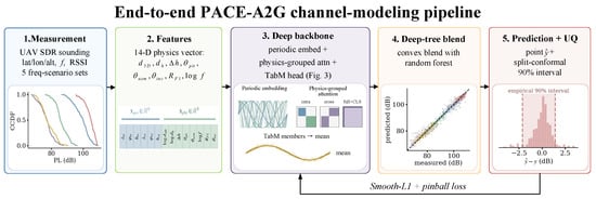
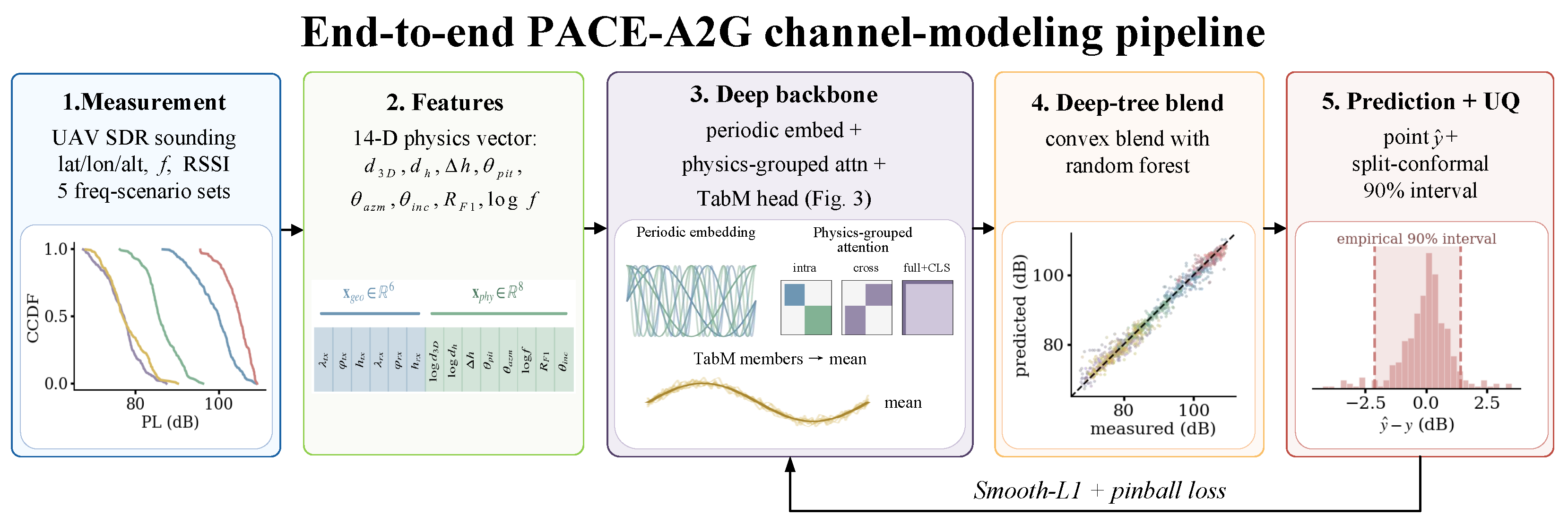
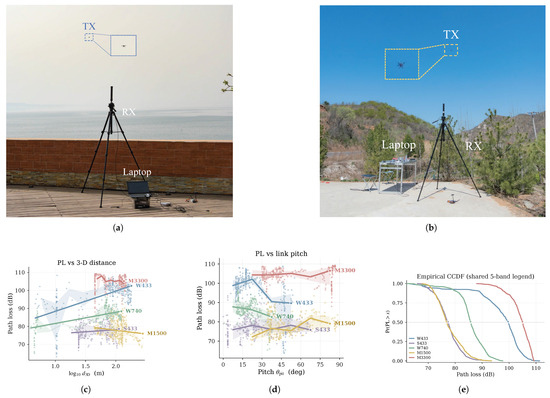
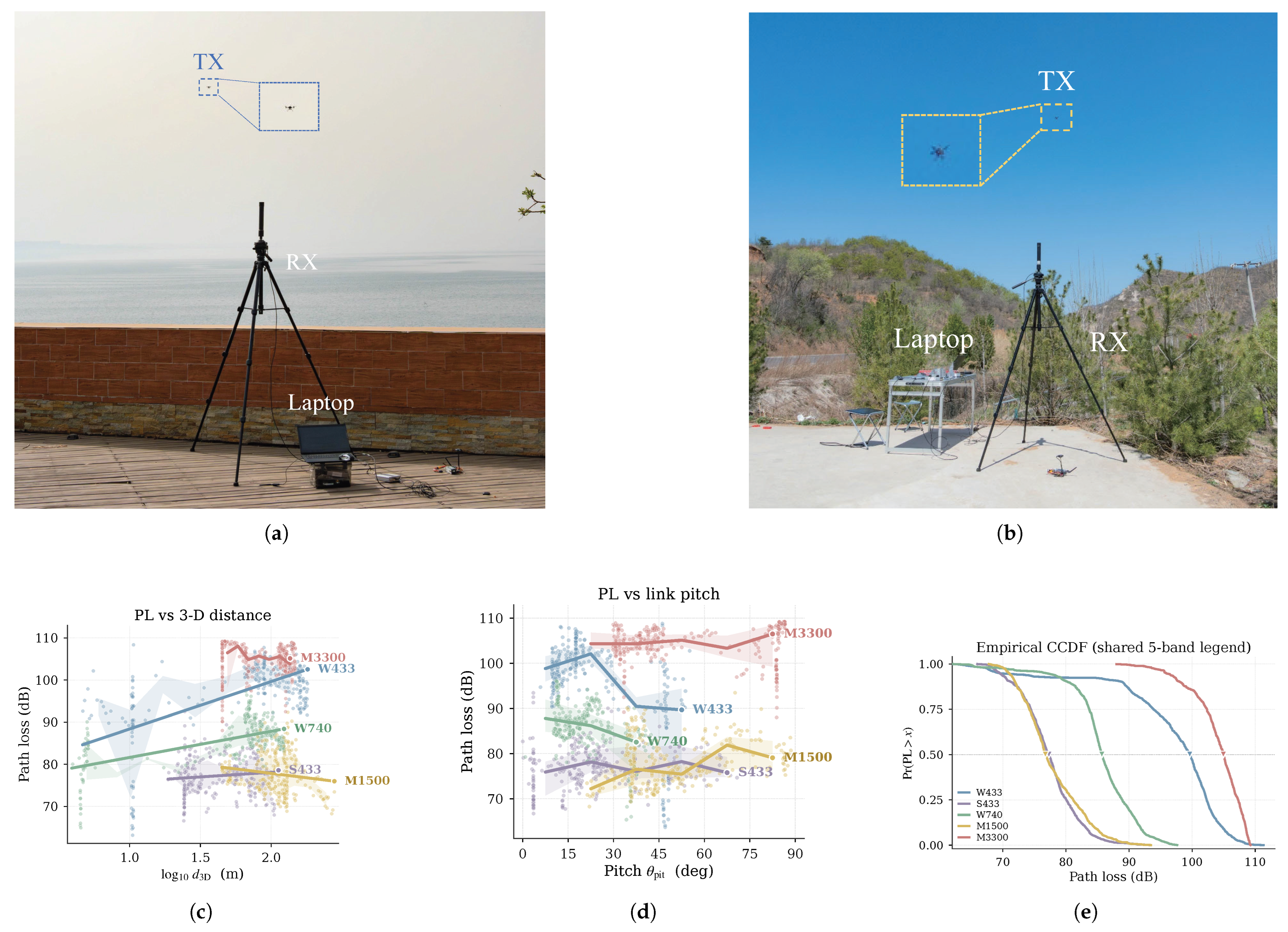
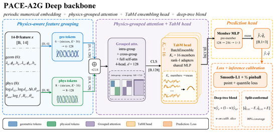
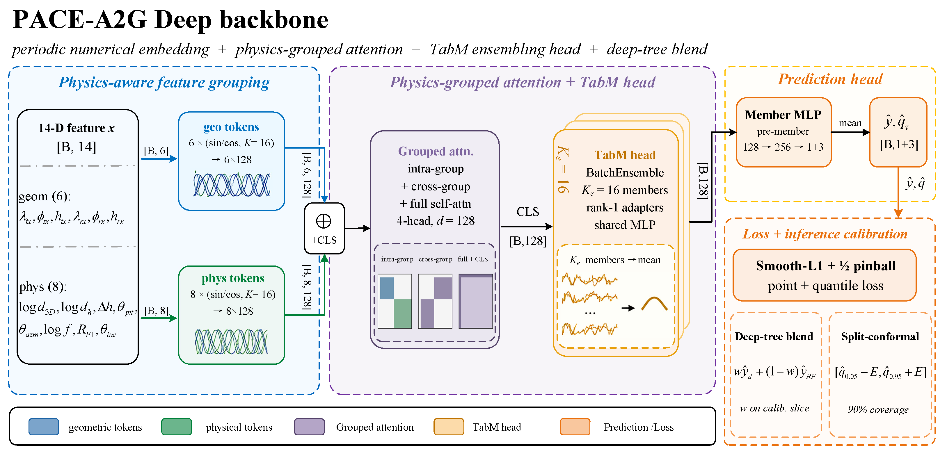
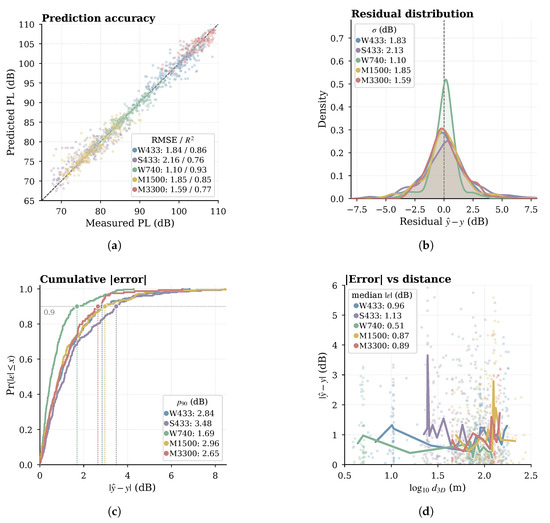
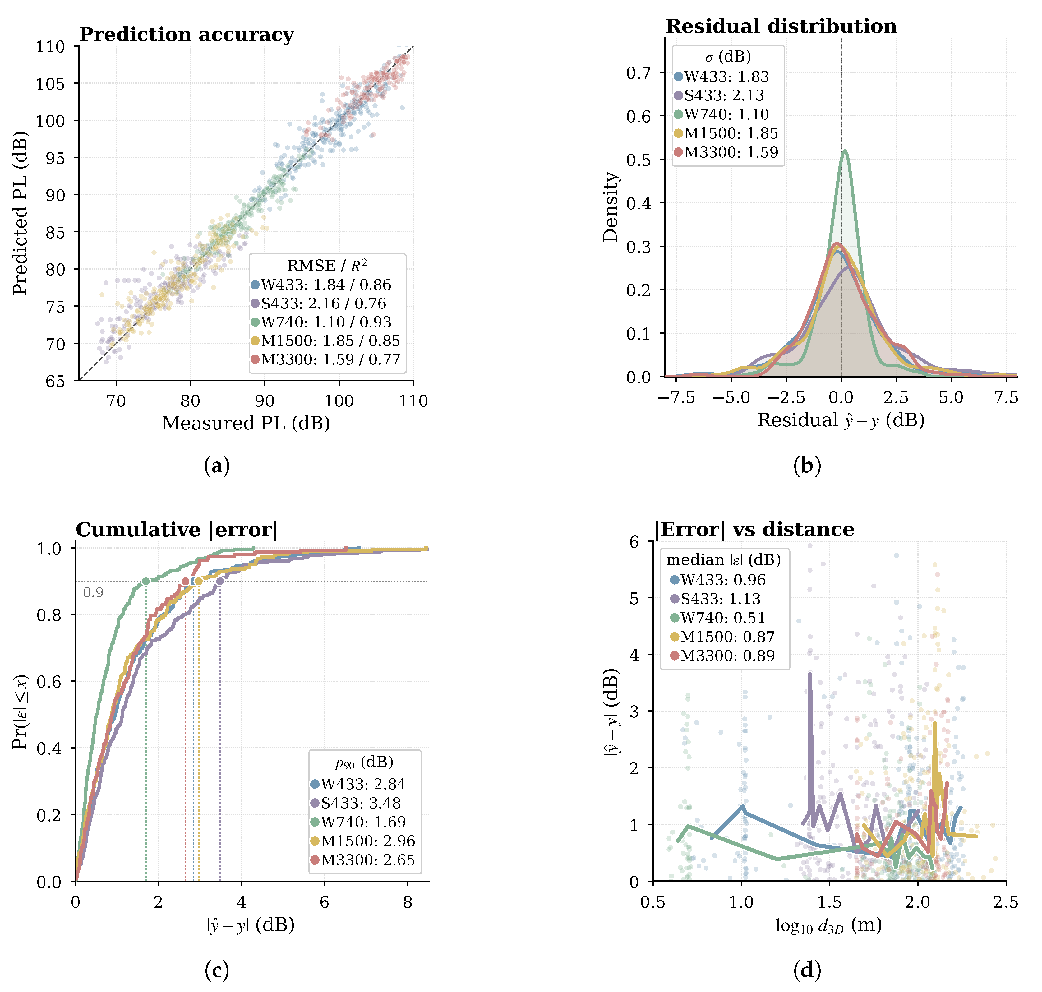
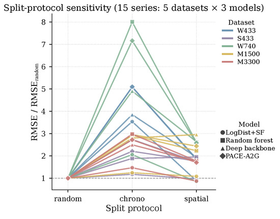
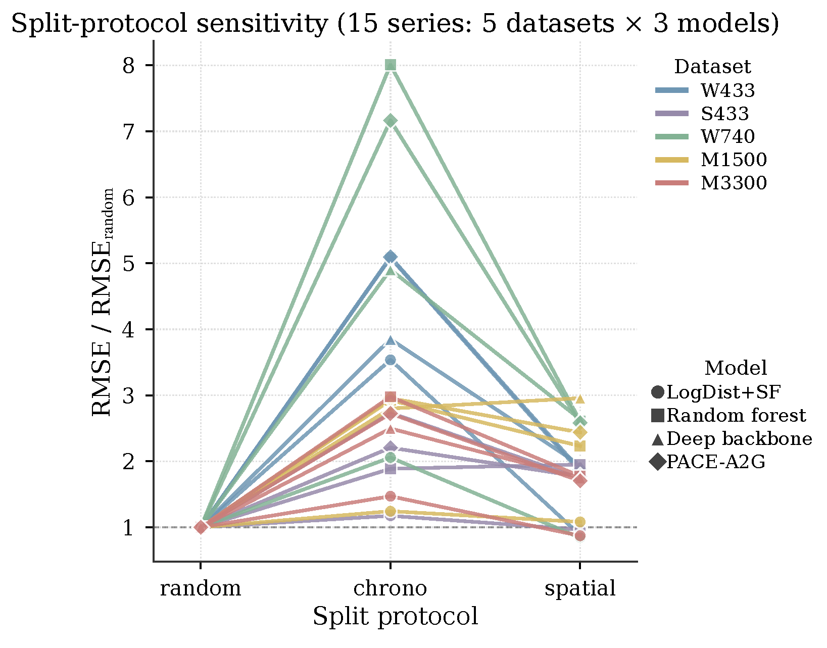
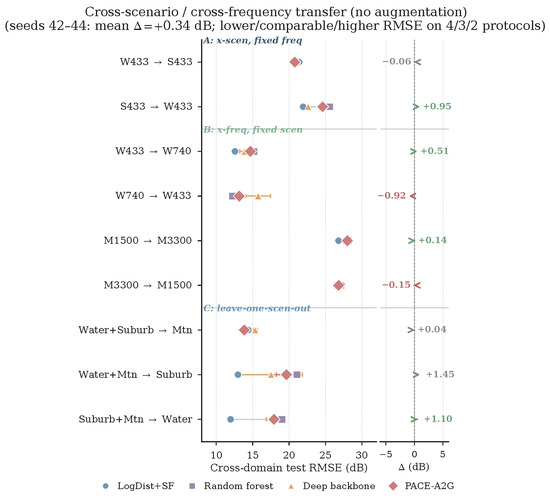
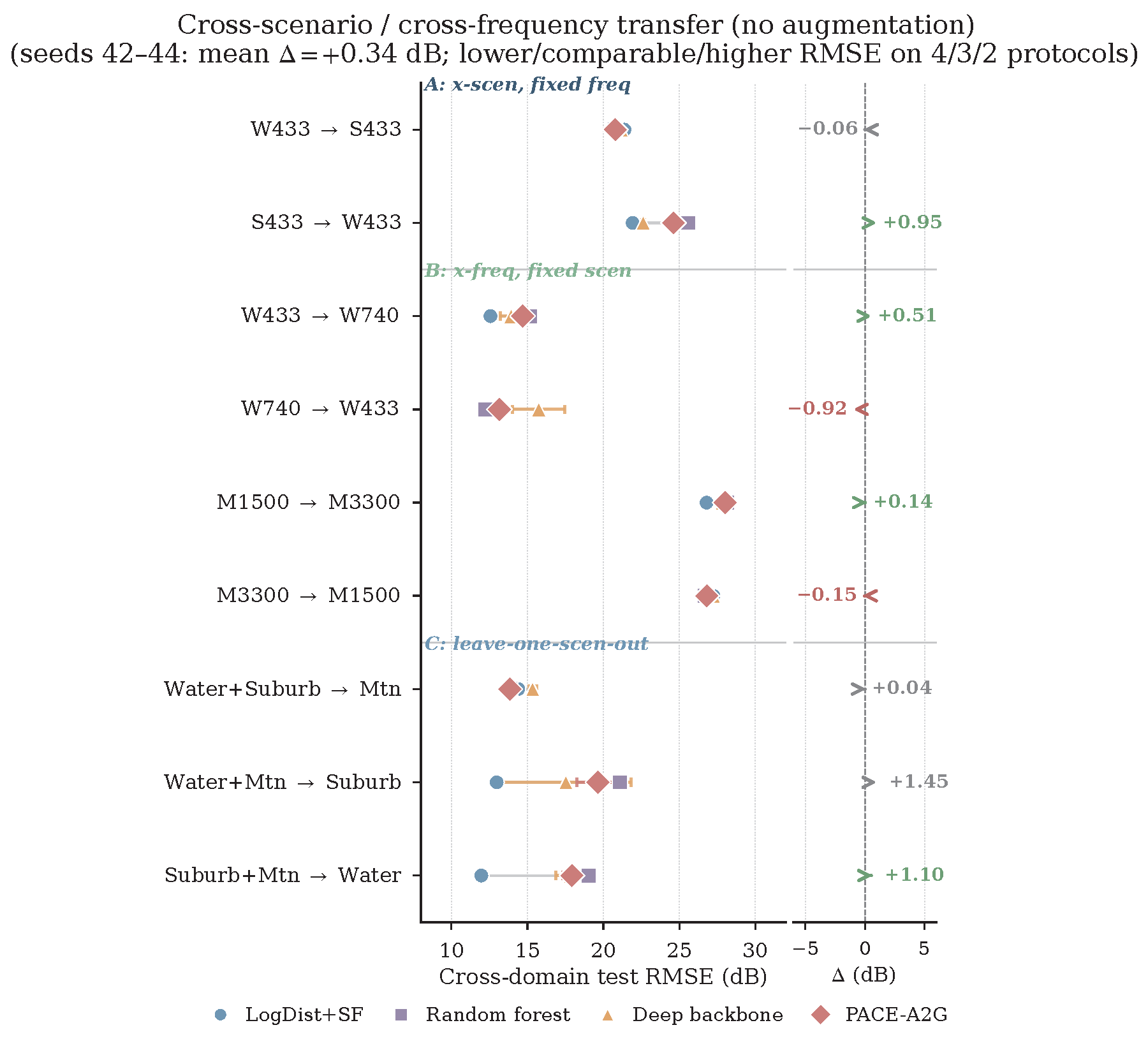
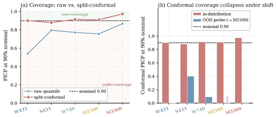
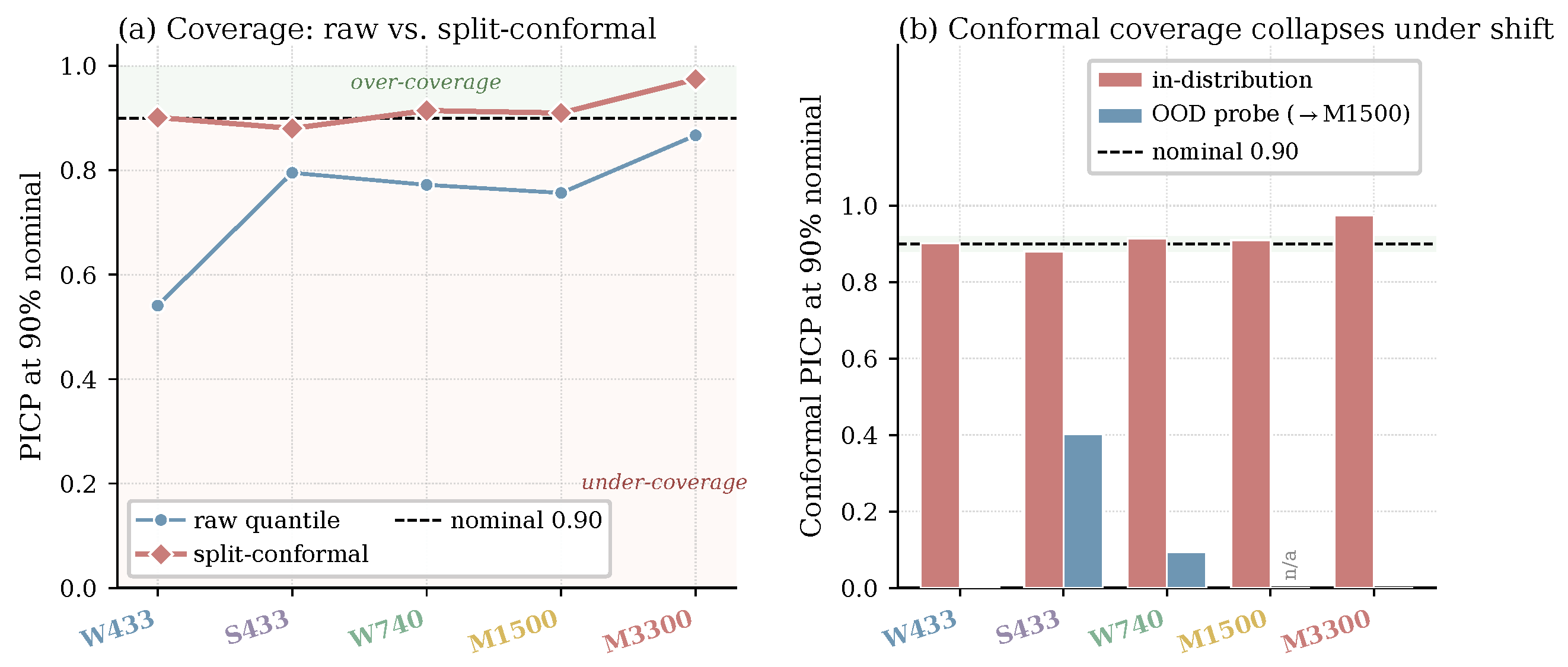
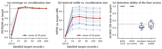
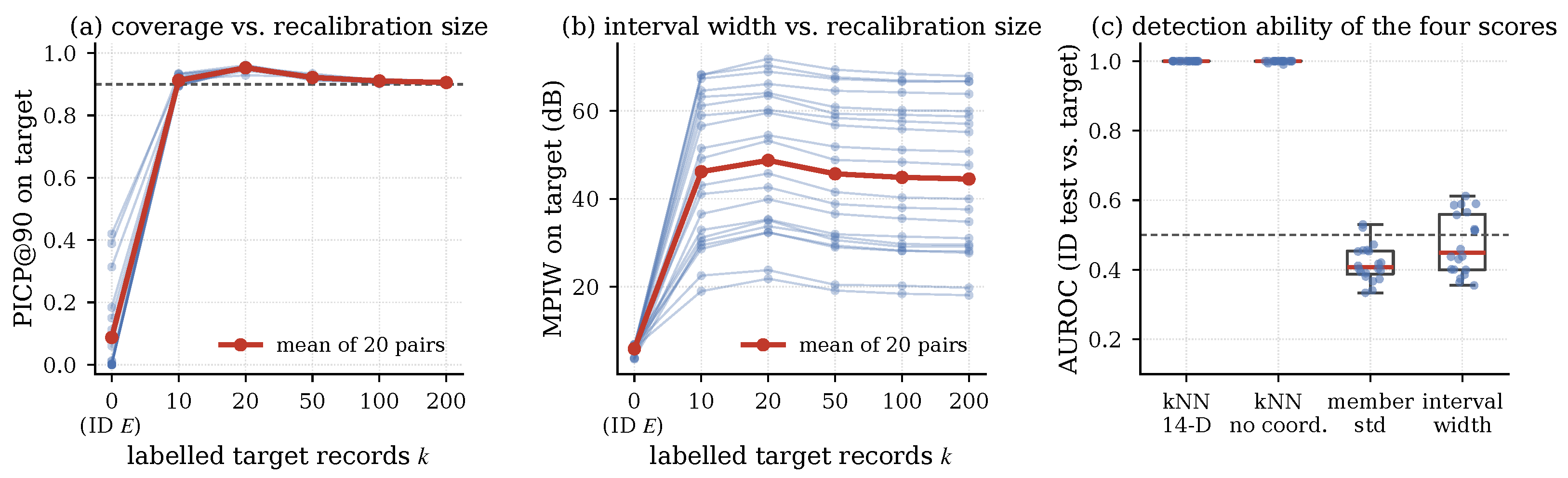
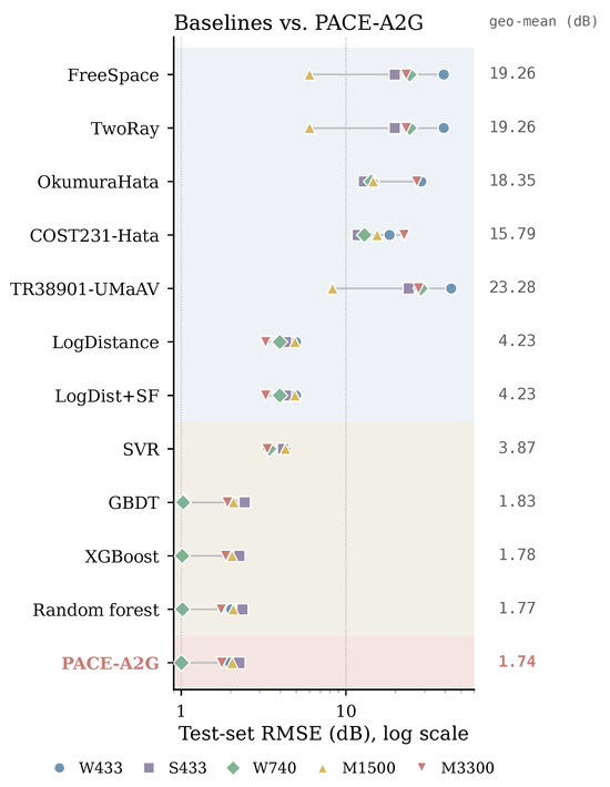
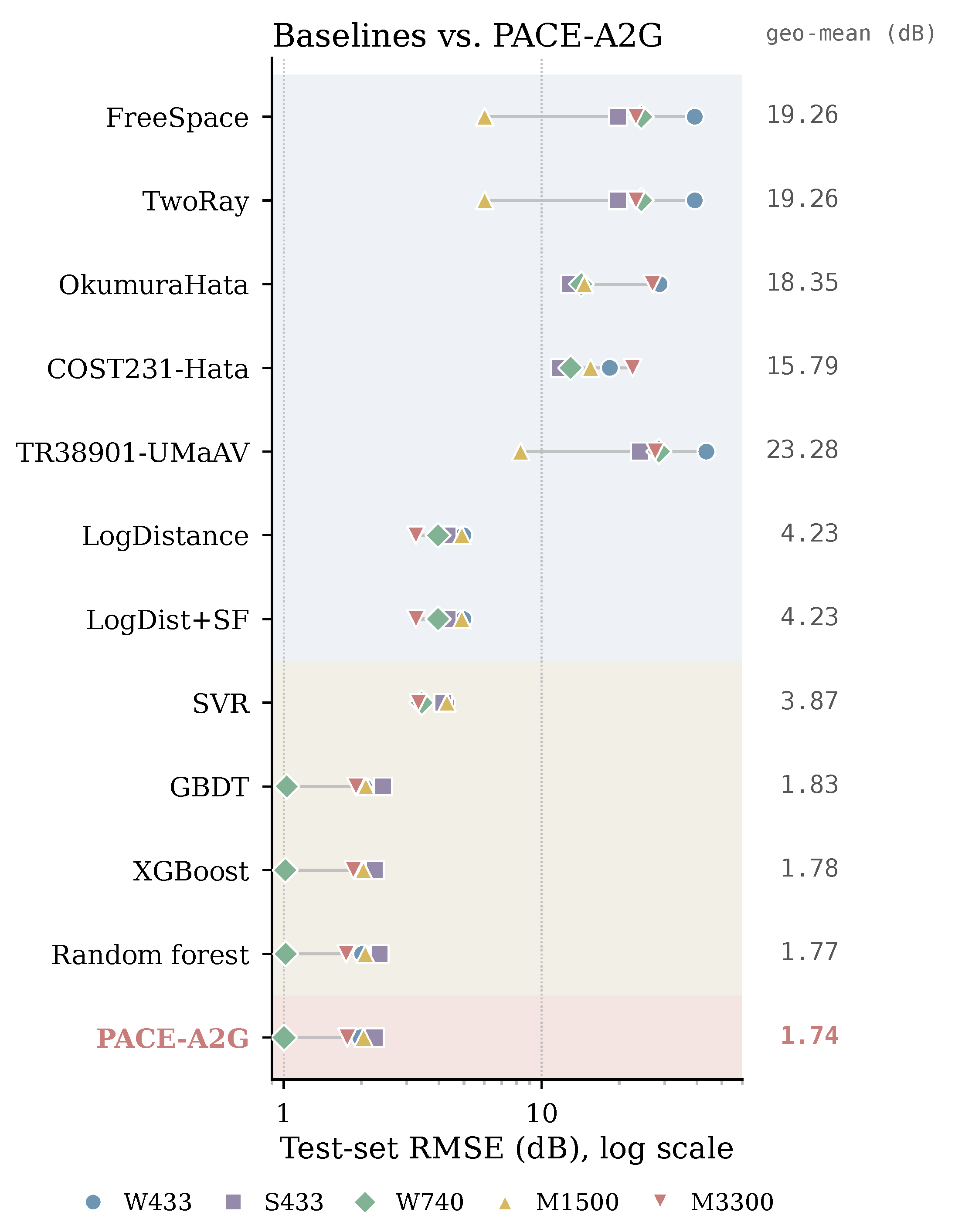

Disclaimer/Publisher’s Note: The statements, opinions and data contained in all publications are solely those of the individual author(s) and contributor(s) and not of MDPI and/or the editor(s). MDPI and/or the editor(s) disclaim responsibility for any injury to people or property resulting from any ideas, methods, instructions or products referred to in the content. |
© 2026 by the authors. Licensee MDPI, Basel, Switzerland. This article is an open access article distributed under the terms and conditions of the Creative Commons Attribution (CC BY) license.