Active Fault-Tolerant Formation Control for Differential-Drive Unmanned Ground Vehicles Under the Separation-Bearing Control Framework

Highlights

What are the main findings?

• A fault-augmented linear error model is developed for differential-drive unmanned ground vehicle formations under the Separation-Bearing Control framework; for a constant-speed reference, the linearization of a stationary operating point is measured, so the model is linear time-invariant, and it explicitly accounts for actuator faults and external disturbances.
• A joint estimation observer and an active fault-compensation controller are designed; the observer reconstructs the fault signal and the controller certifies asymptotic stability of the linear closed-loop error dynamics—hence local asymptotic stability of the nonlinear formation—together with effective recovery of formation performance after actuator faults.

What are the implications of the main findings?

• Online fault estimation and active compensation reject the persistent steady-state offset that fixed-gain robust controllers structurally cannot, while additionally supplying an explicit fault estimate for diagnosis; Monte Carlo, measurement-noise, and modelmismatch studies indicate the behaviour is robust.
• The proposed framework provides a practical approach for improving the reliability and resilience of leader–follower unmanned ground vehicle formations operating in the presence of actuator faults and disturbances.

Abstract

This paper presents an observer-based active fault-tolerant control scheme for leader–follower formations of differential-drive unmanned ground vehicles under the Separation-Bearing Control framework. The relative pose is described by inter-vehicle distance, bearing angle, and heading difference, which are kinematically coupled, so a single actuator fault propagates through all three Separation-Bearing Control channels at once. The nonlinear kinematics are linearized about the rigid-formation operating point; for a constant-speed reference, this operating point is stationary and the resulting fault-augmented error model is linear time-invariant, explicitly accounting for additive actuator faults and bounded external disturbances. A joint estimation observer reconstructs the unmeasured fault signal and filters the measured state with a guaranteed disturbance-attenuation level obtained from a single convex linear matrix inequality, and a state-feedback law with online fault compensation is derived. The linear closed loop is certified asymptotically stable with a prescribed $H_{\infty }$ attenuation bound, which establishes local asymptotic stability of the corresponding equilibrium of the nonlinear formation. Numerical simulations on a three-vehicle circular convoy, together with Monte Carlo, fault-variation, measurement-noise, model-mismatch, and trajectory-change studies, and comparisons against non-fault-tolerant, passive, and integral-action baselines, delineate the specific benefit of online fault reconstruction and active compensation.

1. Introduction

Multi-robot formation control underpins cooperative tasks such as search-and-rescue, logistics, and environmental mapping [1,2]. Among formation paradigms, the leader–follower Separation-Bearing Control (SBC) framework [3] parameterizes relative poses by three scalars—inter-agent distance $L_{li}$, bearing angle ${\psi }_{li}$, and heading difference ${\beta }_{li}$—whose geometric interpretability facilitates formation reconfiguration and analysis [4]. Recent work has addressed collision avoidance [5,6], visibility constraints [7], event-triggered coordination [8], and time-varying delays [9,10]. A structural property of the SBC representation is that $L_{li}$ and ${\psi }_{li}$ are kinematically coupled: a perturbation on either the linear or angular velocity channel of a follower simultaneously corrupts both states, so even a small undetected actuator fault can propagate through multiple SBC state components and risk divergence or inter-vehicle collision.

Differential-drive unmanned ground vehicles (UGVs) are prone to motor degradation, encoder offsets, and wheel slippage, all of which manifest as additive disturbances on the velocity channels [11]. Fault-tolerant control strategies split into passive and active approaches [11]. Passive fault-tolerant control (PFTC) pre-builds robustness into the controller by designing a gain margin sufficient to absorb anticipated faults; however, the required conservatism degrades nominal performance and limits the tolerable fault set. Active fault-tolerant control (AFTC) instead pairs online fault estimation with real-time compensation, achieving wider fault coverage at a lower steady-state performance penalty [12,13]. Observer-based robust and disturbance-rejection methods have proven effective across nonholonomic platforms and multi-agent formations [14,15,16,17,18]. In unmanned aircraft formations, cooperative unknown input observers have been used to simultaneously estimate actuator faults, sensor faults, and external disturbances, yielding fault-tolerant cooperative controllers with provable fixed-time convergence [19]. Robust consensus tracking under concurrent measurement noise and disturbances has likewise been tackled via distributed dual-estimator observer designs, with the approach validated through real-flight multi-UAV experiments [20]. These observer-based strategies have been studied primarily for aerial platforms, and recent work has begun to address wheeled mobile robots as well—for instance, leader–follower formation under actuator loss of effectiveness [21], extended-Kalman-filter fault detection in wheeled-robot consensus [22], and observer-based distributed fault-tolerant consensus [23]. Extending analogous architectures to differential-drive UGV formations governed by a geometric SBC representation nonetheless introduces distinct challenges, as actuator faults couple all three SBC state channels simultaneously through the nonholonomic kinematics. The estimation and synthesis tools drawn upon here—unicycle kinematics, $H_{\infty }$ observers, the change-of-variable linearization of bilinear observer/controller inequalities, and additive-fault compensation via input feedforward—are themselves standard and are not claimed as methodological contributions; the value of the present work lies in adapting and integrating them for the geometrically coupled SBC fault-propagation setting, and in characterizing the resulting behaviour rather than in the estimation machinery per se. Complementary directions include fault compensation for redundant manipulators [24], replay-attack defenses in networked formations [25], and prescribed-time stabilization theory [26].

Against this background, and without claiming absolute priority, we are not aware of prior work that pursues this specific combination for differential-drive UGV formations governed by a Separation-Bearing Control representation. This paper (i) derives a fault-augmented Separation-Bearing Control error model by linearizing about the rigid-formation operating point, which is time-invariant for a constant-speed reference; (ii) designs an $H_{\infty }$ joint estimation observer (JEO) with a guaranteed attenuation bound; (iii) synthesizes a fault-compensating controller that certifies asymptotic stability of the linear closed loop— hence, by the indirect method, local asymptotic stability of the nonlinear formation—together with a prescribed $H_{\infty }$ attenuation bound for the combined closed-loop system; and (iv) validates the resulting scheme on a differential-drive UGV convoy against non-fault-tolerant, passive, and integral-action baselines and under Monte Carlo, fault-variation, measurement-noise, and model-mismatch conditions.

The main contributions of this paper, corresponding to items (i)–(iv) above, are as follows:

• Fault-augmented linear error model for SBC formations. The complete nonlinear Separation-Bearing Control kinematics are derived and linearized about the rigid-formation operating point. For a constant-speed reference, this operating point is stationary, so the Jacobians are constant and the resulting fault-augmented error model is linear time-invariant; additive actuator faults and bounded external disturbances are embedded into it, yielding a description directly amenable to observer-based synthesis. (For a general, non-stationary reference the same construction gives a linear time-varying model, discussed in Section 7.)
• Joint reconstruction of coupled SBC faults. A joint estimation observer is designed to reconstruct the (unmeasured) actuator-fault signal—and, under partial measurement, the state—while attenuating the disturbance influence to a prescribed level through a single convex linear matrix inequality (LMI). Because the fault corrupts all three coupled SBC channels at once, reconstructing it is precisely what enables exact matched compensation.
• Active fault-compensating formation control. A state-feedback control law with online fault compensation is developed so that, in conjunction with the observer, the formation error is restored to its fault-free behaviour; the combined linear closed loop is certified asymptotically stable with a guaranteed disturbance-attenuation level, which establishes local asymptotic stability of the nonlinear formation.
• Comparative and robustness validation on a UGV convoy. A three-vehicle circular-convoy study compares the scheme against non-fault-tolerant, passive, and integral-action baselines—the last of which, like the proposed scheme, can remove the steady-state offset—and Monte Carlo, fault-onset/magnitude/type-variation, measurement-noise, and model-mismatch studies characterize its robustness.

The remainder of this paper is organized as follows. Section 2 derives the SBC fault-augmented linear error model. Section 3 presents the JEO and AFTC controller design. Section 4 reports simulation results for the proposed AFTC scheme. Section 5 presents the comparative study against fixed-gain and integral-action baselines. Section 6 reports the Monte Carlo and robustness studies. Section 7 concludes the paper.

2. System Modeling and Problem Formulation

2.1. Kinematic Model

Consider $N+1$ differential-drive UGVs: leader $R_L$ and followers ${\left\{R_i\right\}}_{i=1}^N$, each obeying the unicycle kinematic model [27,28]

$${\dot{x}}_i=v_i\cos {\theta }_i,{\dot{y}}_i=v_i\sin {\theta }_i,{\dot{\theta }}_i={\omega }_i,$$

(1)

where $x_i$, $y_i$ are Cartesian coordinates, ${\theta }_i$ the heading angle, and $v_i$, ${\omega }_i$ the linear and angular velocities of vehicle $R_i$, respectively. To avoid a bearing-angle singularity when a follower approaches the leader’s geometric center, a virtual reference point

$${\mathbf{p}}_L^d={[x_L-d\cos {\theta }_L,y_L-d\sin {\theta }_L]}^{\top }$$

(2)

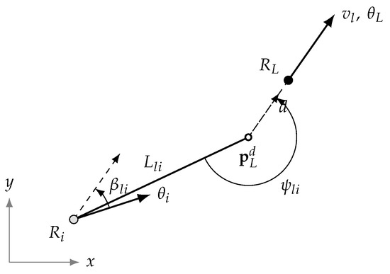
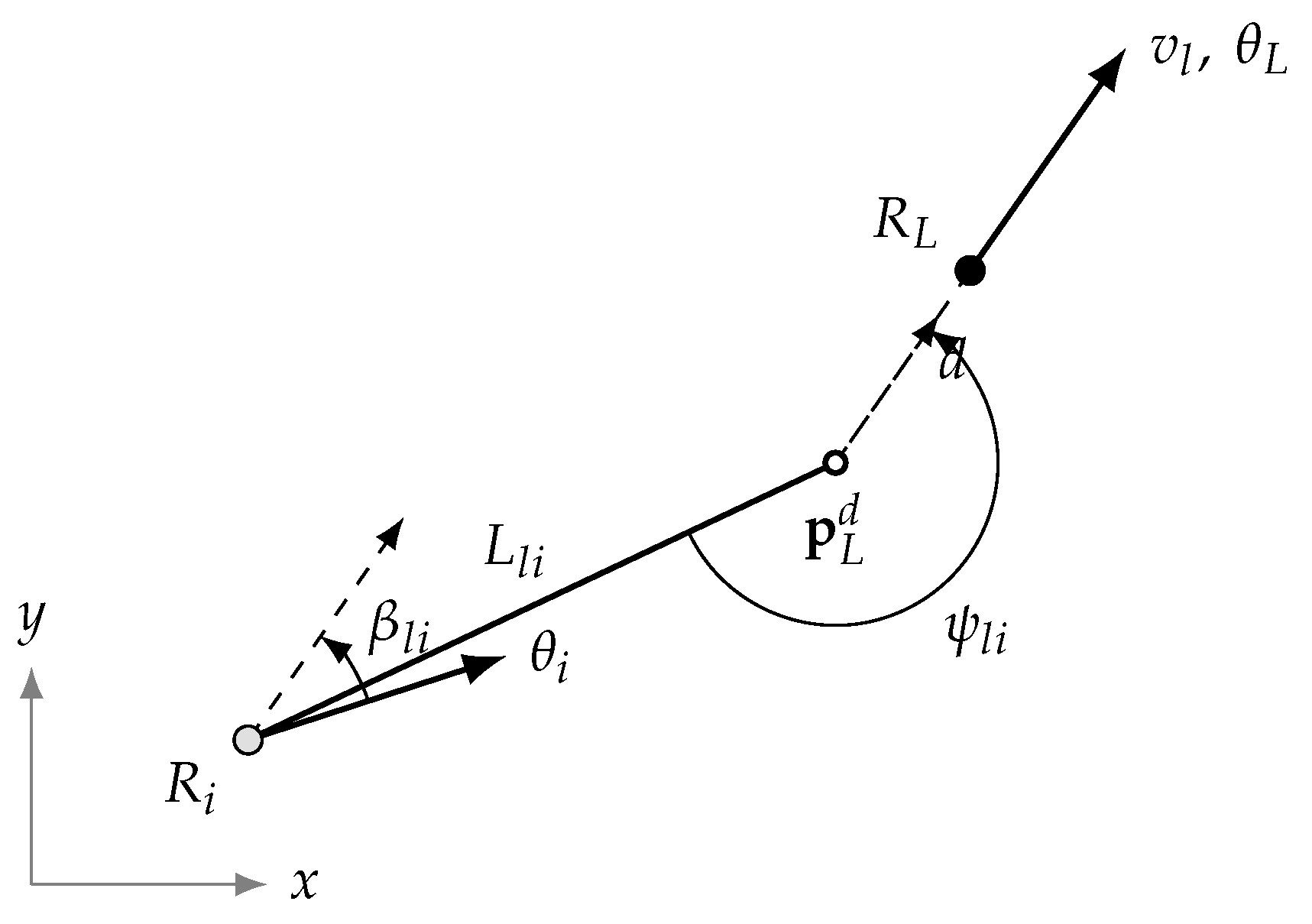
is placed at longitudinal offset $d>0$ ahead of the leader along its heading direction. The leader moves with linear/angular velocity $(v_l,{\omega }_l)$ and heading ${\theta }_L$, and the follower $R_i$ has heading ${\theta }_i$. The resulting leader–follower geometry and the three Separation-Bearing Control quantities used throughout the paper are illustrated in Figure 1.

Figure 1. Leader–follower geometry under the Separation-Bearing Control framework.

2.2. SBC Formation State and Nonlinear Dynamics

The SBC state [3] is defined as the triplet ${\mathit{\chi }}_i={[L_{li},{\psi }_{li},{\beta }_{li}]}^{\top }$, where $L_{li}=\parallel {\mathbf{p}}_L^d-{\mathbf{p}}_i\parallel$ is the Euclidean separation from $R_i$ to ${\mathbf{p}}_L^d$, ${\psi }_{li}$ is the bearing angle from $R_i$ to ${\mathbf{p}}_L^d$ measured from the leader’s velocity direction, and ${\beta }_{li}={\theta }_L-{\theta }_i$ is the heading difference. The leader tracks the virtual reference point ${\mathbf{p}}_L^d={\mathbf{p}}_L-d{[\cos {\theta }_L,\sin {\theta }_L]}^{\top }$, whose inertial velocity is ${\dot{\mathbf{p}}}_L^d={[v_l\cos {\theta }_L+d{\omega }_l\sin {\theta }_L,v_l\sin {\theta }_L-d{\omega }_l\cos {\theta }_L]}^{\top }$. Writing the line-of-sight vector as ${\mathbf{p}}_i-{\mathbf{p}}_L^d={[L_{lix},L_{liy}]}^{\top }$ with the Cartesian decomposition $L_{lix}=-L_{li}\cos ({\psi }_{li}+{\theta }_L)$, $L_{liy}=-L_{li}\sin ({\psi }_{li}+{\theta }_L)$ and differentiating along trajectories of (1) gives ${\dot{L}}_{lix}=v_i\cos {\theta }_i-v_l\cos {\theta }_L-d{\omega }_l\sin {\theta }_L$ and ${\dot{L}}_{liy}=v_i\sin {\theta }_i-v_l\sin {\theta }_L+d{\omega }_l\cos {\theta }_L$. Projecting these onto the line-of-sight and its normal via ${\dot{L}}_{li}=-\cos {\alpha }_{li}{\dot{L}}_{lix}-\sin {\alpha }_{li}{\dot{L}}_{liy}$ and $L_{li}{\dot{\alpha }}_{li}=\sin {\alpha }_{li}{\dot{L}}_{lix}-\cos {\alpha }_{li}{\dot{L}}_{liy}$, where ${\alpha }_{li}={\psi }_{li}+{\theta }_L$ and ${\dot{\psi }}_{li}={\dot{\alpha }}_{li}-{\omega }_l$, and substituting ${\theta }_i={\theta }_L-{\beta }_{li}$ yields the SBC kinematics

$$\begin{array}{cc}\hfill {\dot{L}}_{li}& =v_l\cos {\psi }_{li}-v_i\cos {\varphi }_{li}-d{\omega }_l\sin {\psi }_{li},\hfill \end{array}$$

(3)

$$\begin{array}{cc}\hfill {\dot{\psi }}_{li}& =\frac{1}{L_{li}}\left(v_i\sin {\varphi }_{li}-v_l\sin {\psi }_{li}-d{\omega }_l\cos {\psi }_{li}\right)-{\omega }_l,\hfill \end{array}$$

(4)

$$\begin{array}{cc}\hfill {\dot{\beta }}_{li}& ={\omega }_l-{\omega }_i,\hfill \end{array}$$

(5)

with composite angle ${\varphi }_{li}={\psi }_{li}+{\beta }_{li}$. Throughout, $v_l$ and ${\omega }_l$ denote the leader linear and angular velocities (equivalently $v_L$ and ${\omega }_L$ of $R_L$; the subscript l is reserved for the leader) and are distinct from the exogenous disturbance w introduced later in (7). In particular, the standalone term $-{\omega }_l$ in the bearing rate (4) appears because ${\psi }_{li}$ is measured relative to the rotating leader velocity direction, so the leader turn rate ${\omega }_l$ must be subtracted to obtain the bearing rate in the inertial frame. Consistent with the projection geometry, the leader velocity $v_l$ enters through the line-of-sight angle ${\psi }_{li}$ while the follower velocity $v_i$ enters through ${\varphi }_{li}$; the $d{\omega }_l$ terms originate from the leader angular rate acting on the offset reference point ${\mathbf{p}}_L^d$. The follower angular rate ${\omega }_i$ enters only through ${\dot{\beta }}_{li}$ in (5), and thereafter couples into $L_{li},{\psi }_{li}$ through the state dynamics rather than by direct feedthrough.

2.3. Fault-Augmented Linear Error Model at the Operating Point

Let ${\mathit{\chi }}_i^d={[L_{li}^d,{\psi }_{li}^d,{\beta }_{li}^d]}^{\top }$ be the desired SBC state with nominal input ${\mathbf{u}}_i^d={[v_i^d,{\omega }_i^d]}^{\top }$. Define the formation-error state $\mathbf{x}={\mathit{\chi }}_i-{\mathit{\chi }}_i^d$ and control deviation $\overline{\mathbf{u}}={\mathbf{u}}_i-{\mathbf{u}}_i^d$. A first-order Taylor expansion of the nonlinear kinematics (3)–(5) about $({\mathit{\chi }}_i^d,{\mathbf{u}}_i^d)$ retains the constant and first-order terms and discards the second- and higher-order remainder of order $O(\parallel \mathbf{x}{\parallel }^2+\parallel \overline{\mathbf{u}}{\parallel }^2)$, which is negligible in a neighbourhood of the operating point. This gives $\dot{\mathbf{x}}\approx \mathbf{A}\mathbf{x}+\mathbf{B}\overline{\mathbf{u}}$, where $\mathbf{A}$ and $\mathbf{B}$ are the Jacobians of the kinematics with respect to the state and the input, respectively, evaluated at the operating point [15]

$$\mathbf{A}=\left[\begin{array}{ccc}0& a_{12}& v_i^d\sin {\varphi }_{li}^d\\ {\displaystyle \frac{-a_{12}}{{\left(L_{li}^d\right)}^2}}& {\displaystyle \frac{a_{22}}{L_{li}^d}}& {\displaystyle \frac{v_i^d\cos {\varphi }_{li}^d}{L_{li}^d}}\\ 0& 0& 0\end{array}\right],\mathbf{B}=\left[\begin{array}{cc}-\cos {\varphi }_{li}^d& 0\\ {\displaystyle \frac{\sin {\varphi }_{li}^d}{L_{li}^d}}& 0\\ 0& -1\end{array}\right],$$

(6)

where ${\varphi }_{li}^d={\psi }_{li}^d+{\beta }_{li}^d$ and

$$\begin{array}{cc}\hfill a_{12}& =v_i^d\sin {\varphi }_{li}^d-v_l\sin {\psi }_{li}^d-d{\omega }_l\cos {\psi }_{li}^d=\partial {\dot{L}}_{li}/\partial {\psi }_{li},\hfill \\ \hfill a_{22}& =v_i^d\cos {\varphi }_{li}^d-v_l\cos {\psi }_{li}^d+d{\omega }_l\sin {\psi }_{li}^d.\hfill \end{array}$$

Two points follow directly from (3)–(5). First, $\partial {\dot{L}}_{li}/\partial {\psi }_{li}=a_{12}$ carries units of $[\mathrm{m}/\mathrm{s}]$ as required, and no spurious $1/L_{li}^d$ factor appears in this entry. Second, because both ${\dot{L}}_{li}$ and ${\dot{\psi }}_{li}$ depend on ${\beta }_{li}$ through ${\varphi }_{li}$, the third column of $\mathbf{A}$ is generically nonzero, with $\partial {\dot{L}}_{li}/\partial {\beta }_{li}=v_i^d\sin {\varphi }_{li}^d$ and $\partial {\dot{\psi }}_{li}/\partial {\beta }_{li}=v_i^d\cos {\varphi }_{li}^d/L_{li}^d$. In $\mathbf{B}$, the follower angular-rate channel ${\omega }_i$ appears only in ${\dot{\beta }}_{li}={\omega }_l-{\omega }_i$, so the second column of $\mathbf{B}$ is ${[0,0,-1]}^{\top }$; the $d(·)$ terms present in (3) and (4) stem from the leader input ${\omega }_l$ and are captured inside $a_{12},a_{22}$ rather than in the follower input matrix.

Evaluating $\mathbf{A}$ at a rigid-formation operating point, where the stationarity conditions $\mathbf{f}({\mathit{\chi }}_i^d,{\mathbf{u}}_i^d)=\mathbf{0}$ give $v_i^d\sin {\varphi }_{li}^d-v_l\sin {\psi }_{li}^d-d{\omega }_l\cos {\psi }_{li}^d=L_{li}^d{\omega }_l$, $v_i^d\cos {\varphi }_{li}^d-v_l\cos {\psi }_{li}^d+d{\omega }_l\sin {\psi }_{li}^d=0$ and ${\omega }_i^d={\omega }_l$, the Jacobian reduces to the compact form $a_{12}=L_{li}^d{\omega }_l$, $a_{22}=0$, so that $A_{21}=-{\omega }_l/L_{li}^d$. The off-diagonal entries of $\mathbf{A}$ thus capture the L–$\psi$ coupling, while the corrected $\mathbf{B}$ shows that an ${\omega }_i$ actuator fault acts directly only on ${\beta }_{li}$ and couples into $L_{li},{\psi }_{li}$ through the state dynamics, not through input feedthrough.

Incorporating additive actuator fault $\mathbf{f}\left(t\right)\in {\mathbb{R}}^2$ and a scalar ${\mathcal{L}}_2$ disturbance $w\left(t\right)\in \mathbb{R}$ (aggregating unmodeled kinematic and measurement perturbations), the fault-augmented error model is

$$\dot{\mathbf{x}}\left(t\right)=\mathbf{A}\mathbf{x}+\mathbf{B}\overline{\mathbf{u}}+\mathbf{E}\mathbf{f}+\mathbf{D}w,\mathbf{y}=\mathbf{C}\mathbf{x},$$

(7)

Here, $\mathbf{E}\in {\mathbb{R}}^{3\times 2}$ is the fault-distribution matrix: its columns specify the directions in the error state space along which the two fault components $\mathbf{f}\left(t\right)={[f_1,f_2]}^{\top }$ act, exactly as $\mathbf{B}$ specifies how the control deviation $\overline{\mathbf{u}}$ enters. Because the faults modeled here are additive actuator faults on the commanded $(v_i,{\omega }_i)$ channels, $\mathbf{E}$ shares the entry directions of $\mathbf{B}$; the specific choice $\mathbf{E}=\mathbf{B}$ (the matched case) is formalized in Assumption 3 and is what renders exact fault cancellation possible. The column $\mathbf{D}\in {\mathbb{R}}^{3\times 1}$ is the disturbance-input direction of the scalar signal $w\left(t\right)$, and $\mathbf{C}={\mathbf{I}}_3$ (full-state measurement).

Remark 1 (Time-invariance of the operating-point model). 

Equation (7) is written with a time argument because, for a general reference, the desired SBC state ${\mathit{\chi }}_i^d\left(t\right)$ and nominal input ${\mathbf{u}}_i^d\left(t\right)$ vary along the trajectory, so the Jacobians $\mathbf{A}\left(t\right), \mathbf{B}\left(t\right)$ of (6) are time-varying and the model is linear time-varying (LTV). For the case of interest here—a rigid formation tracking a constant-speed reference (Section 4)—the operating point is stationary: $\mathbf{f}({\mathit{\chi }}_i^d,{\mathbf{u}}_i^d)=\mathbf{0}$ has a constant solution (with the compact values $a_{12}=L_{li}^d{\omega }_l$, $a_{22}=0$ above), so $\mathbf{A}, \mathbf{B}, \mathbf{E}=\mathbf{B}$, and $\mathbf{D}$ are constant and (7) is linear time-invariant (LTI). All of the observer and controller synthesis below is carried out for this constant LTI model; accordingly, the stability certificates use time-invariant notions (Hurwitz matrices, constant Lyapunov matrices, and a single LMI evaluated at the operating point), which are the appropriate tools for a constant $\mathbf{A}$. The genuinely time-varying case is not treated analytically here: the constant design can be applied in a frozen-time (pointwise) sense, and its extension via a parameter-dependent Lyapunov function or gain scheduling is left to future work (Section 7); a trajectory-change scenario in which the operating point drifts is examined empirically in Section 6.

The following three conditions underpin the observer and controller design.

Assumption 1 (Observability). 

At the operating point the pair $(\mathbf{A},\mathbf{C})$ is observable (equivalently, for a time-varying reference, $\left(\mathbf{A}\right(t),\mathbf{C})$ is uniformly observable along the desired trajectory).

Assumption 2 (Slowly Varying Fault). 

$\parallel \dot{\mathbf{f}}\parallel \le f_d$; the observer design uses the working approximation $\dot{\mathbf{f}}\approx \mathbf{0}$.

Assumption 3 (Additive Actuator Fault/Matching Condition). 

The fault acts additively through the control input channel, so that $\mathbf{E}=\mathbf{B}$. Since $\mathbf{B}$ has full column rank ($\mathrm{rank}\mathbf{B}=2$), this gives $\mathrm{rank}\left(\mathbf{B}\right)=\mathrm{rank}\left(\right[\mathbf{B},\mathbf{E}\left]\right)$ and $\mathbf{B}{\mathbf{B}}^{†}\mathbf{E}=\mathbf{E}$, ${\mathbf{B}}^{†}\mathbf{B}={\mathbf{I}}_2$, so fault compensation is exact.

Remark 2. 

Because the corrected $\mathbf{B}$ in (6) has only two columns and full column rank, taking $\mathbf{E}$ as “the first two columns of $\mathbf{B}$” is identical to setting $\mathbf{E}=\mathbf{B}$. We state this explicitly. Physically it models an additive actuator fault: a loss of effectiveness or bias in the commanded $(v_i,{\omega }_i)$, e.g., wheel-slip, encoder bias, or drive-train offset, which necessarily enters the plant through the same channel as the control input. Under $\mathbf{E}=\mathbf{B}$ the compensation term ${\mathbf{B}}^{†}\mathbf{E}\widehat{\mathbf{f}}$ reduces to $\widehat{\mathbf{f}}$, so the compensating control is ${\overline{\mathbf{u}}}_{\mathrm{comp}}=-\widehat{\mathbf{f}}$: the estimate is fed back directly to cancel the fault at its point of entry, which is exactly the desired behaviour for matched additive faults.

The restriction $\mathbf{E}=\mathbf{B}$ is essential to exact cancellation but is not required for the observer, which reconstructs $(\mathbf{x},\mathbf{f})$ for any $\mathbf{E}$ of full column rank. When $\mathbf{E}\ne \mathbf{B}$ (unmatched actuator faults, or sensor/process faults entering through directions outside $\mathrm{range}\left(\mathbf{B}\right)$), the matching condition fails and $\mathbf{B}{\mathbf{B}}^{†}\mathbf{E}\ne \mathbf{E}$; the residual $(\mathbf{I}-\mathbf{B}{\mathbf{B}}^{†})\mathbf{E}\widehat{\mathbf{f}}$ cannot be removed by input compensation and must instead be attenuated by the $H_{\infty }$ feedback channel. In that case, the present scheme still guarantees bounded formation error with the prescribed attenuation ${\gamma }_c$ but no longer achieves asymptotic fault cancellation; handling unmatched or sensor faults exactly would require augmenting the input with additional actuation or redesigning the compensator, which we leave as future work (see Section 7).

For the circular reference trajectory used in Section 4, Assumption 1 is satisfied whenever $v_l>0$ and $L_{li}^d\ne 0$, and step faults and gradual encoder drift satisfy Assumption 2 after the onset transient; any residual $\dot{\mathbf{f}}$ is captured by the $H_{\infty }$ bound ${\gamma }_{\mathrm{obs}}$.

Problem Statement. 

Under (7) and Assumptions 1–3, design (a) a JEO reconstructing $\mathbf{x}\left(t\right)$ and $\mathbf{f}\left(t\right)$ with $H_{\infty }$ attenuation ${\gamma }_{\mathrm{obs}}$, and (b) an AFTC law driving $\mathbf{x}\left(t\right)\to \mathbf{0}$ with $H_{\infty }$ attenuation ${\gamma }_c$.

2.4. Modeling Simplifications and Implementation Limitations

The tractability of the model (7) and of the synthesis in Section 3 rests on a set of simplifying assumptions relating the idealized description to a physical differential-drive platform. We list them explicitly, since several of them also delimit the conditions under which the guarantees apply and may constitute implementation limitations.

(A1)

Kinematic (unicycle) actuation. The plant is the first-order kinematics (1): vehicle mass, inertia, wheel/motor dynamics, and tire–ground interaction are neglected, and the commanded velocities $(v_i,{\omega }_i)$ are assumed to be realized instantaneously. On hardware, these commands are the set-points of an inner velocity loop of finite bandwidth, so the present results describe the outer formation loop under the standard time-scale-separation assumption.

(A2)

Fault class. Motor degradation, encoder offset, and wheel slip are lumped into a single additive, matched fault $\mathbf{f}\left(t\right)$ acting on the velocity channels (Assumption 3) that is slowly varying (Assumption 2). Multiplicative loss-of-effectiveness, unmatched actuator faults, and sensor faults are not canceled exactly and are only attenuated through the $H_{\infty }$ channel (Remark 2).

(A3)

Feedback signals. Full-state SBC feedback $\mathbf{y}=\mathbf{C}\mathbf{x}$ with $\mathbf{C}={\mathbf{I}}_3$ is available, i.e., the relative pose $(L_{li},{\psi }_{li},{\beta }_{li})$ is measurable (e.g., by onboard range/bearing sensing or external localization) and, in the nominal design, noise-free. Measurement noise and partial output measurement are treated only empirically (Section 6.3) and by the output-feedback extension noted in Remark 3.

(A4)

Aggregated disturbance. All unmodeled kinematic and measurement perturbations are aggregated into a single bounded ${\mathcal{L}}_2$ signal $w\left(t\right)$ entering through the fixed, known direction $\mathbf{D}$.

(A5)

Local, operating-point linearization. The synthesis uses the first-order model about the rigid-formation operating point, which is valid on a neighborhood of the desired formation; for a constant-speed reference, this point is stationary and the model is LTI (Remark 1). Large excursions and genuinely time-varying references lie outside the certified region (Remark 4).

(A6)

Architecture. Each follower uses only its own relative state to the leader and is assumed to have ideal, delay-free access to the leader reference; inter-follower communication, network delays, and explicit collision avoidance are outside the present scope.

(A7)

Unsaturated control. The stability and $H_{\infty }$ certificates of Section 3 are derived for the unsaturated control law; actuator saturation is enforced in simulation and its effect verified a posteriori (Section 4.5).

3. Observer and Controller Design

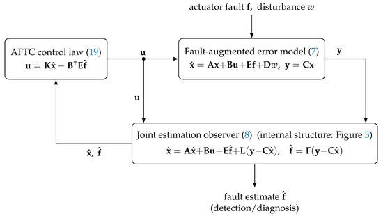
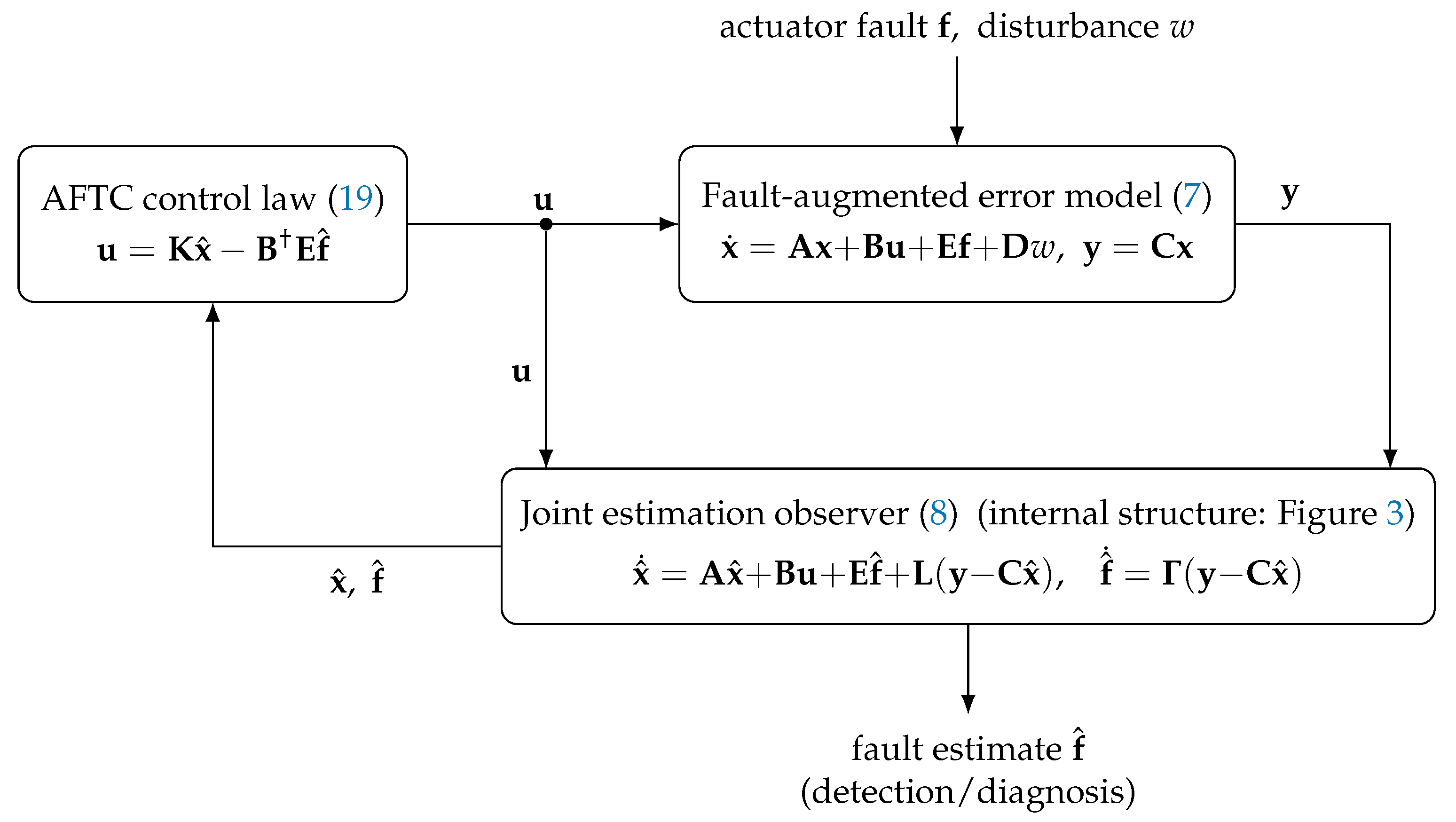
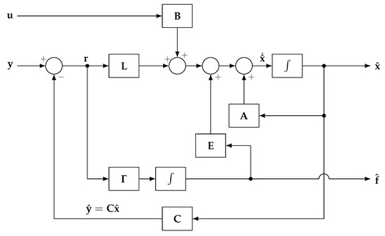
The overall active fault-tolerant architecture is shown in Figure 2. A word on notation is in order first. From this section onward, the control signal is written $\mathbf{u}$ rather than the deviation variable $\overline{\mathbf{u}}={\mathbf{u}}_i-{\mathbf{u}}_i^d$ used in the modeling of Section 2: once the dynamics have been reduced to the error model (7), the absolute input ${\mathbf{u}}_i$ and the nominal input ${\mathbf{u}}_i^d$ no longer appear, so the bar becomes redundant and is dropped for readability. Thus $\mathbf{u}$ throughout Section 4.2 and Section 4 denotes exactly the deviation $\overline{\mathbf{u}}$ of the error model, i.e., the quantity produced by the control law (19); the command actually applied to follower $R_i$ remains ${\mathbf{u}}_i={\mathbf{u}}_i^d+\mathbf{u}$.

Figure 2. Block diagram of the observer-based active fault-tolerant control scheme, with the control-input tap indicated by the filled circle.

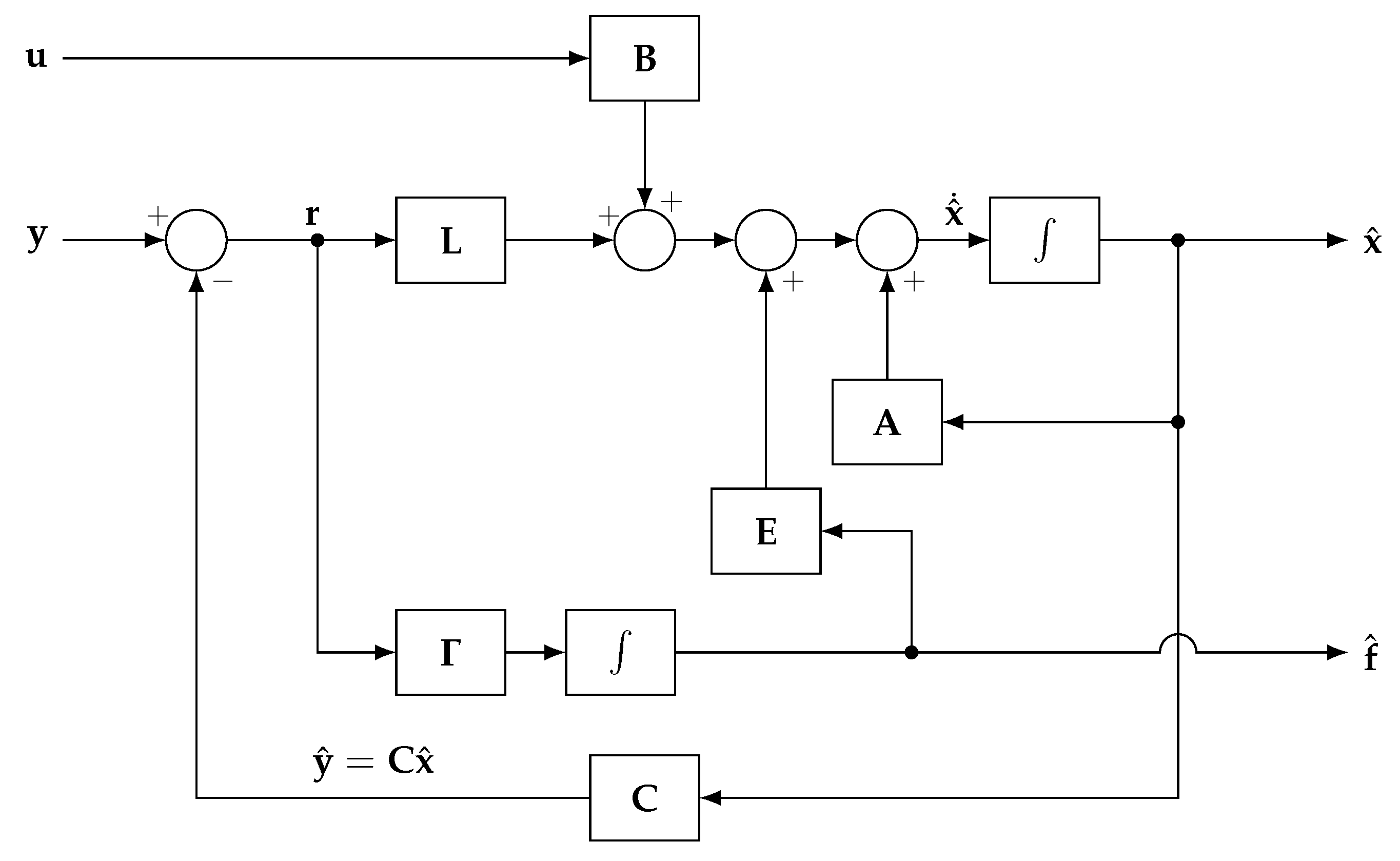
The joint estimation observer (JEO) is a model-based (Luenberger-type) estimator: it propagates a copy of the plant model (7) and corrects that copy by output injection. It is therefore driven by the two input signals that appear on the right-hand side of (8)—the applied control input $\mathbf{u}$ and the measured output $\mathbf{y}$—and both are shown explicitly in Figure 2. The input $\mathbf{u}$ is not an unknown to be reconstructed but a signal generated by the controller itself; it is consequently tapped from the controller output and fed to the observer, which is precisely what makes the shared control term cancel when the observer is subtracted from the plant to form the estimation-error dynamics (9). From $(\mathbf{u},\mathbf{y})$, the JEO reconstructs the state $\widehat{\mathbf{x}}$ and the actuator fault $\widehat{\mathbf{f}}$; the reconstructed fault is fed forward through the compensation term $-{\mathbf{B}}^{†}\mathbf{E}\widehat{\mathbf{f}}$ of the control law, while the reconstructed state drives the nominal feedback $\mathbf{K}\widehat{\mathbf{x}}$. The internal wiring of the observer is detailed separately in Figure 3. Because $\widehat{\mathbf{f}}$ is available directly at the observer output, it also serves as a diagnostic signal for fault detection and isolation, independently of its role in the compensation term above. The remainder of this section derives the two gain sets, $(\mathbf{L},\mathbf{\Gamma })$ and $\mathbf{K}$, that appear in the diagram.

Figure 3. Internal structure of the joint estimation observer (8), detailed in the text; the semicircular hop denotes crossing lines that are not connected.

3.1. Joint Estimation Observer

Building on joint state–fault observer design in [29,30], the proposed JEO is

$$\dot{\widehat{\mathbf{x}}}=\mathbf{A}\widehat{\mathbf{x}}+\mathbf{B}\mathbf{u}+\mathbf{E}\widehat{\mathbf{f}}+\mathbf{L}(\mathbf{y}-\mathbf{C}\widehat{\mathbf{x}}),\dot{\widehat{\mathbf{f}}}=\mathbf{\Gamma }(\mathbf{y}-\mathbf{C}\widehat{\mathbf{x}}),$$

(8)

with state gain $\mathbf{L}\in {\mathbb{R}}^{3\times 3}$ and fault-estimation gain $\mathbf{\Gamma }\in {\mathbb{R}}^{2\times 3}$. The fault estimator $\dot{\widehat{\mathbf{f}}}=\mathbf{\Gamma }(\mathbf{y}-\mathbf{C}\widehat{\mathbf{x}})$ is an output-injection integrator: it continuously adjusts the fault estimate according to the measurement residual, driving the estimation error to zero as the residual decays.

The internal structure of (8) is detailed in Figure 3. Both inputs enter on the left: the known control input $\mathbf{u}$ is passed through $\mathbf{B}$ into the state channel, so that the observer replicates the forcing that the controller applies to the plant, whereas the measured output $\mathbf{y}$ is compared with its estimate $\widehat{\mathbf{y}}=\mathbf{C}\widehat{\mathbf{x}}$ to form the residual $\mathbf{r}=\mathbf{y}-\mathbf{C}\widehat{\mathbf{x}}$. The residual is the only correction signal in the observer and is shared by its two channels: it is injected into the state channel through $\mathbf{L}$ and integrated in the fault channel through $\mathbf{\Gamma }$. The two channels are coupled in both directions—the fault estimate $\widehat{\mathbf{f}}$ re-enters the state channel through $\mathbf{E}$, while $\widehat{\mathbf{x}}$ shapes $\widehat{\mathbf{f}}$ through the residual—which is the coupling described by the augmented matrix ${\mathbf{A}}_{\mathrm{obs}}$ of (12) below, and the reason the two gains are synthesized jointly from a single LMI rather than in sequence.

Remark 3 (Role of the observer under full-state measurement). 

With $\mathbf{C}={\mathbf{I}}_3$ the formation-error state $\mathbf{x}$ is measured directly, so the state estimate $\widehat{\mathbf{x}}$ is not required for state reconstruction; in the noise-free case, $\widehat{\mathbf{x}}\to \mathbf{x}$ and, taken alone, the state channel is redundant. The essential and non-redundant function of the observer is fault reconstruction: the fault $\mathbf{f}$ is not measured, and the output-injection integrator $\dot{\widehat{\mathbf{f}}}=\mathbf{\Gamma }(\mathbf{y}-\mathbf{C}\widehat{\mathbf{x}})$ recovers it from the residual. The joint (state-and-fault) form is nonetheless retained for three reasons: (i) it produces the clean residual $\mathbf{y}-\mathbf{C}\widehat{\mathbf{x}}$ that drives the fault integrator and yields a single convex LMI for both gains $(\mathbf{L},\mathbf{\Gamma })$; (ii) when the measurement is corrupted by disturbance w or sensor noise, the state channel filters these before they reach the fault estimator, which materially improves fault reconstruction under noise (Section 6); and (iii) the same design carries over unchanged to output-feedback settings $\mathbf{C}\ne {\mathbf{I}}_3$ (partial measurement), where the state estimate becomes indispensable. The observer is therefore best read as a fault estimator with an auxiliary state filter, rather than as a state observer.

To examine how the JEO estimates converge, define the state estimation error ${\mathbf{e}}_s=\mathbf{x}-\widehat{\mathbf{x}}$ and the fault estimation error ${\mathbf{e}}_f=\mathbf{f}-\widehat{\mathbf{f}}$. Subtracting the first equation of (8) from the plant (7) cancels the shared control term, leaving

$${\dot{\mathbf{e}}}_s=(\mathbf{A}-\mathbf{L}\mathbf{C}){\mathbf{e}}_s+\mathbf{E}{\mathbf{e}}_f+\mathbf{D}w.$$

(9)

Since the estimator in (8) satisfies $\dot{\widehat{\mathbf{f}}}=\mathbf{\Gamma }\mathbf{C}{\mathbf{e}}_s$, differentiating ${\mathbf{e}}_f=\mathbf{f}-\widehat{\mathbf{f}}$ gives

$${\dot{\mathbf{e}}}_f=-\mathbf{\Gamma }\mathbf{C}{\mathbf{e}}_s+\dot{\mathbf{f}}.$$

(10)

The term $\dot{\mathbf{f}}$ enters as a bounded exogenous signal: under Assumption 2 it satisfies $\parallel \dot{\mathbf{f}}\parallel \le f_d$, and its effect is absorbed into the $H_{\infty }$ attenuation bound ${\gamma }_{\mathrm{obs}}$ established below. Writing (9) and (10) in the augmented error state $\mathit{\xi }={[{\mathbf{e}}_s^{\top },{\mathbf{e}}_f^{\top }]}^{\top }\in {\mathbb{R}}^5$ with composite disturbance $\tilde{\mathbf{w}}={[w,{\dot{\mathbf{f}}}^{\top }]}^{\top }\in {\mathbb{R}}^3$ yields the augmented estimation-error dynamics

$$\dot{\mathit{\xi }}={\mathbf{A}}_{\mathrm{obs}}\mathit{\xi }+{\mathbf{E}}_{\xi }\tilde{\mathbf{w}},$$

(11)

with

$${\mathbf{A}}_{\mathrm{obs}}=\left[\begin{array}{cc}\mathbf{A}-\mathbf{L}\mathbf{C}& \mathbf{E}\\ -\mathbf{\Gamma }\mathbf{C}& \mathbf{0}\end{array}\right],{\mathbf{E}}_{\xi }=\left[\begin{array}{cc}\mathbf{D}& \mathbf{0}\\ \mathbf{0}& \mathbf{I}\end{array}\right].$$

(12)

Theorem 1 ($H_{\infty }$ Observer Gain Synthesis). 

Consider the augmented error dynamics (11). For prescribed ${\gamma }_{\mathrm{obs}}>0$, if there exist $\mathbf{P}={\mathbf{P}}^{\top }>0$ and $\mathbf{Y}$ satisfying

$$\left[\begin{array}{ccc}\mathbf{P}{\mathbf{A}}_{\mathrm{sys}}-\mathbf{Y}{\mathbf{C}}_{\mathrm{sys}}+{(·)}^{\top }& \mathbf{P}{\mathbf{E}}_{\xi }& \mathbf{I}\\ {\mathbf{E}}_{\xi }^{\top }\mathbf{P}& -{\gamma }_{\mathrm{obs}}^2\mathbf{I}& \mathbf{0}\\ \mathbf{I}& \mathbf{0}& -\mathbf{I}\end{array}\right]<0,$$

(13)

where ${\mathbf{A}}_{\mathrm{sys}}=\left[\begin{array}{cc}\mathbf{A}& \mathbf{E}\\ \mathbf{0}& \mathbf{0}\end{array}\right]$, ${\mathbf{C}}_{\mathrm{sys}}=[\mathbf{C},\mathbf{0}]$, then ${\mathbf{A}}_{\mathrm{obs}}$ is Hurwitz, ${\int }_0^{\infty }{\parallel \mathit{\xi }\parallel }^{2}dt\le {\gamma }_{\mathrm{obs}}^2{\int }_0^{\infty }{\parallel \tilde{\mathbf{w}}\parallel }^{2}dt$, and the gains are recovered as ${[{\mathbf{L}}^{\top },{\mathbf{\Gamma }}^{\top }]}^{\top }={\mathbf{P}}^{-1}\mathbf{Y}$.

Proof. 

Choose the Lyapunov function candidate $V\left(\mathit{\xi }\right)={\mathit{\xi }}^{\top }\mathbf{P}\mathit{\xi }$ with $\mathbf{P}>0$. Differentiating V along the trajectories of (11) yields

$$\dot{V}\left(\mathit{\xi }\right)={\mathit{\xi }}^{\top }\left({\mathbf{A}}_{\mathrm{obs}}^{\top }\mathbf{P}+\mathbf{P}{\mathbf{A}}_{\mathrm{obs}}\right)\mathit{\xi }+{\tilde{\mathbf{w}}}^{\top }{\mathbf{E}}_{\xi }^{\top }\mathbf{P}\mathit{\xi }+{\mathit{\xi }}^{\top }\mathbf{P}{\mathbf{E}}_{\xi }\tilde{\mathbf{w}}.$$

(14)

To enforce the prescribed $H_{\infty }$ performance, introduce the Hamiltonian $\mathcal{H}=\dot{V}\left(\mathit{\xi }\right)+{\mathit{\xi }}^{\top }\mathit{\xi }-{\gamma }_{\mathrm{obs}}^2{\tilde{\mathbf{w}}}^{\top }\tilde{\mathbf{w}}$ and require $\mathcal{H}<0$. Written as a quadratic form in ${[{\mathit{\xi }}^{\top },{\tilde{\mathbf{w}}}^{\top }]}^{\top }$, this reads

$${\left[\begin{array}{c}\mathit{\xi }\\ \tilde{\mathbf{w}}\end{array}\right]}^{\top }\left[\begin{array}{cc}{\mathbf{A}}_{\mathrm{obs}}^{\top }\mathbf{P}+\mathbf{P}{\mathbf{A}}_{\mathrm{obs}}+\mathbf{I}& \mathbf{P}{\mathbf{E}}_{\xi }\\ {\mathbf{E}}_{\xi }^{\top }\mathbf{P}& -{\gamma }_{\mathrm{obs}}^2\mathbf{I}\end{array}\right]\left[\begin{array}{c}\mathit{\xi }\\ \tilde{\mathbf{w}}\end{array}\right]<0,$$

(15)

so the central matrix must be strictly negative definite. Applying the Schur complement to the identity term contained in the $(1,1)$ block, (15) is equivalent to

$$\left[\begin{array}{ccc}{\mathbf{A}}_{\mathrm{obs}}^{\top }\mathbf{P}+\mathbf{P}{\mathbf{A}}_{\mathrm{obs}}& \mathbf{P}{\mathbf{E}}_{\xi }& \mathbf{I}\\ {\mathbf{E}}_{\xi }^{\top }\mathbf{P}& -{\gamma }_{\mathrm{obs}}^2\mathbf{I}& \mathbf{0}\\ \mathbf{I}& \mathbf{0}& -\mathbf{I}\end{array}\right]<0.$$

(16)

Inequality (16) is bilinear in $\mathbf{P}$ and the gains through the product $\mathbf{P}{\mathbf{A}}_{\mathrm{obs}}$. To linearize it, decompose the observer matrix as

$${\mathbf{A}}_{\mathrm{obs}}={\mathbf{A}}_{\mathrm{sys}}-\mathcal{L}{\mathbf{C}}_{\mathrm{sys}},\mathcal{L}=\left[\begin{array}{c}\mathbf{L}\\ \mathbf{\Gamma }\end{array}\right],$$

(17)

with the stacked observer gain $\mathcal{L}$ and ${\mathbf{A}}_{\mathrm{sys}}$, ${\mathbf{C}}_{\mathrm{sys}}$ as defined in the statement, so that $\mathbf{P}{\mathbf{A}}_{\mathrm{obs}}=\mathbf{P}{\mathbf{A}}_{\mathrm{sys}}-\mathbf{P}\mathcal{L}{\mathbf{C}}_{\mathrm{sys}}$. The change of variable $\mathbf{Y}=\mathbf{P}\mathcal{L}$ removes the bilinearity, giving $\mathbf{P}{\mathbf{A}}_{\mathrm{obs}}=\mathbf{P}{\mathbf{A}}_{\mathrm{sys}}-\mathbf{Y}{\mathbf{C}}_{\mathrm{sys}}$; substituting this expression into (16) reproduces exactly the LMI (13). Once $\mathbf{P}$ and $\mathbf{Y}$ are obtained, partitioning $\mathbf{Y}={[{\mathbf{W}}_L^{\top },{\mathbf{W}}_{\mathsf{\Gamma }}^{\top }]}^{\top }$ conformably with $\mathcal{L}$ recovers the gains as

$$\left[\begin{array}{c}\mathbf{L}\\ \mathbf{\Gamma }\end{array}\right]={\mathbf{P}}^{-1}\mathbf{Y}={\mathbf{P}}^{-1}\left[\begin{array}{c}{\mathbf{W}}_L\\ {\mathbf{W}}_{\mathsf{\Gamma }}\end{array}\right].$$

(18)

Finally, setting $\tilde{\mathbf{w}}\equiv \mathbf{0}$ in (15) gives $\dot{V}\le -{\parallel \mathit{\xi }\parallel }^2<0$ for every $\mathit{\xi }\ne \mathbf{0}$, so ${\mathbf{A}}_{\mathrm{obs}}$ is Hurwitz and the augmented error system is asymptotically stable. Integrating $\mathcal{H}\le 0$ from 0 to ∞ under zero initial conditions establishes the attenuation bound ${\int }_0^{\infty }{\parallel \mathit{\xi }\parallel }^{2}dt\le {\gamma }_{\mathrm{obs}}^2{\int }_0^{\infty }{\parallel \tilde{\mathbf{w}}\parallel }^{2}dt$. □

3.2. Active Fault-Tolerant Controller

Given JEO estimates $\widehat{\mathbf{x}}$ and $\widehat{\mathbf{f}}$, the AFTC law is

$$\mathbf{u}=\underset{\mathrm{nominal}}{\underbrace{\mathbf{K}\widehat{\mathbf{x}}}}-\underset{\mathrm{fault} \mathrm{compensation}}{\underbrace{{\mathbf{B}}^{†}\mathbf{E}\widehat{\mathbf{f}}}},$$

(19)

where $\mathbf{K}\in {\mathbb{R}}^{2\times 3}$ and ${\mathbf{B}}^{†}$ is the Moore–Penrose pseudoinverse. To design $\mathbf{K}$ for the actual closed-loop system, the AFTC law (19) is substituted simultaneously into the plant (7) and into the observer (8).

Step 1: Closed-loop plant dynamics. Substituting (19) into (7), writing $\widehat{\mathbf{x}}=\mathbf{x}-{\mathbf{e}}_s$ and $\widehat{\mathbf{f}}=\mathbf{f}-{\mathbf{e}}_f$, and invoking the matching condition $\mathbf{B}{\mathbf{B}}^{†}\mathbf{E}=\mathbf{E}$ (Assumption 3) yields

$$\dot{\mathbf{x}}=(\mathbf{A}+\mathbf{B}\mathbf{K})\mathbf{x}-\mathbf{B}\mathbf{K}{\mathbf{e}}_s+\mathbf{E}{\mathbf{e}}_f+\mathbf{D}w.$$

(20)

The true fault $\mathbf{E}\mathbf{f}$ cancels exactly from the plant; only the fault estimation error ${\mathbf{e}}_f$ persists as a residual driving term.

Step 2: Observer dynamics under the control law. Substituting (19) into the first equation of (8) and using $\mathbf{B}{\mathbf{B}}^{†}\mathbf{E}=\mathbf{E}$ again gives

$$\dot{\widehat{\mathbf{x}}}=(\mathbf{A}+\mathbf{B}\mathbf{K})\widehat{\mathbf{x}}+\mathbf{L}\mathbf{C}{\mathbf{e}}_s.$$

(21)

The estimated fault $\widehat{\mathbf{f}}$ vanishes entirely because the compensation term $-{\mathbf{B}}^{†}\mathbf{E}\widehat{\mathbf{f}}$ fed into the observer is exactly canceled by $\mathbf{E}\widehat{\mathbf{f}}$.

Step 3: Estimation-error dynamics. Subtracting (21) from (20) gives

$${\dot{\mathbf{e}}}_s=(\mathbf{A}-\mathbf{L}\mathbf{C}){\mathbf{e}}_s+\mathbf{E}{\mathbf{e}}_f+\mathbf{D}w,$$

(22)

which is independent of $\widehat{\mathbf{x}}$ and $\mathbf{K}$ and coincides with the ${\mathbf{e}}_s$-subsystem of (11).

Step 4: Combined closed-loop system. Stacking (21) and (22) with the combined state $\mathbf{z}={[{\widehat{\mathbf{x}}}^{\top },{\mathbf{e}}_s^{\top }]}^{\top }\in {\mathbb{R}}^6$ gives the combined closed-loop system

$$\dot{\mathbf{z}}={\mathbf{A}}_e\mathbf{z}+{\mathbf{D}}_e{\mathbf{v}}_e,{\mathbf{A}}_e=\left[\begin{array}{cc}\mathbf{A}+\mathbf{B}\mathbf{K}& \mathbf{L}\mathbf{C}\\ \mathbf{0}& \mathbf{A}-\mathbf{L}\mathbf{C}\end{array}\right],{\mathbf{D}}_e=\left[\begin{array}{cc}\mathbf{0}& \mathbf{0}\\ \mathbf{E}& \mathbf{D}\end{array}\right],$$

(23)

with composite disturbance ${\mathbf{v}}_e={[{\mathbf{e}}_f^{\top },w]}^{\top }\in {\mathbb{R}}^3$. The block-triangular structure of ${\mathbf{A}}_e$ enables independent stability analysis of the observer and controller subsystems.

Theorem 2 (Closed-Loop Stability and $H_{\infty }$ Attenuation). 

Let ${\mathbf{E}}_d=[\mathbf{E},\mathbf{D}]$. For a prescribed ${\gamma }_c>0$, suppose there exist matrices ${\mathbf{X}}_1={\mathbf{X}}_1^{\top }\succ 0$, ${\mathbf{P}}_2={\mathbf{P}}_2^{\top }\succ 0$ and ${\mathbf{Y}}_c$ such that

$$\left[\begin{array}{cccc}{\mathbf{\Psi }}_{11}& \mathbf{L}\mathbf{C}& \mathbf{0}& {\mathbf{X}}_1\\ \ast & {\mathbf{\Phi }}_{22}& {\mathbf{P}}_2{\mathbf{E}}_d& \mathbf{I}\\ \ast & \ast & -{\gamma }_c^2\mathbf{I}& \mathbf{0}\\ \ast & \ast & \ast & -\mathbf{I}\end{array}\right]\prec 0,$$

(24)

where ${\mathbf{\Psi }}_{11}=\mathbf{A}{\mathbf{X}}_1+{\mathbf{X}}_1{\mathbf{A}}^{\top }+\mathbf{B}{\mathbf{Y}}_c+{\mathbf{Y}}_c^{\top }{\mathbf{B}}^{\top }$ and ${\mathbf{\Phi }}_{22}={(\mathbf{A}-\mathbf{L}\mathbf{C})}^{\top }{\mathbf{P}}_2+{\mathbf{P}}_2(\mathbf{A}-\mathbf{L}\mathbf{C})$. Here, $\mathbf{L}$ is the observer gain fixed by Theorem 1, whereas ${\mathbf{P}}_2$ is an independent decision variable of (24) (it is not inherited from the observer Lyapunov matrix $\mathbf{P}$). Consequently, (24) is a genuine LMI, jointly convex in $({\mathbf{X}}_1,{\mathbf{P}}_2,{\mathbf{Y}}_c)$. Then, with $\mathbf{K}={\mathbf{Y}}_c{\mathbf{X}}_1^{-1}$:

(i) 

The linear combined system (23) is asymptotically stable—indeed globally exponentially stable, being a Hurwitz LTI system—when ${\mathbf{v}}_e\equiv \mathbf{0}$, so $\mathbf{x}\left(t\right)\to \mathbf{0}$;

(ii) 

${\int }_0^{\infty }{\parallel \mathbf{x}\parallel }^{2}dt\le {\gamma }_c^2{\int }_0^{\infty }{\parallel {\mathbf{v}}_e\parallel }^{2}dt$ under zero initial conditions.

Proof. 

Choose the block-diagonal Lyapunov function

$$V\left(\mathbf{z}\right)={\widehat{\mathbf{x}}}^{\top }{\mathbf{P}}_1\widehat{\mathbf{x}}+{\mathbf{e}}_s^{\top }{\mathbf{P}}_2{\mathbf{e}}_s,{\mathbf{P}}_1={\mathbf{X}}_1^{-1}\succ 0,{\mathbf{P}}_2\succ 0,$$

(25)

and define the Hamiltonian $\mathcal{H}=\dot{V}+{\parallel \mathbf{x}\parallel }^2-{\gamma }_c^2{\parallel {\mathbf{v}}_e\parallel }^2$ with $\mathbf{x}=\widehat{\mathbf{x}}+{\mathbf{e}}_s$. Differentiating V with respect to time and substituting the closed-loop derivatives $\dot{\widehat{\mathbf{x}}}$ and ${\dot{\mathbf{e}}}_s$ given by (21) and (22)—that is, evaluating $\dot{V}={\dot{\widehat{\mathbf{x}}}}^{\top }{\mathbf{P}}_1\widehat{\mathbf{x}}+{\widehat{\mathbf{x}}}^{\top }{\mathbf{P}}_1\dot{\widehat{\mathbf{x}}}+{\dot{\mathbf{e}}}_s^{\top }{\mathbf{P}}_2{\mathbf{e}}_s+{\mathbf{e}}_s^{\top }{\mathbf{P}}_2{\dot{\mathbf{e}}}_s$ along the trajectories of the combined closed loop—and keeping the output term ${\parallel \mathbf{x}\parallel }^2={\parallel \widehat{\mathbf{x}}+{\mathbf{e}}_s\parallel }^2$ unexpanded so that the Schur complement can later be applied to it cleanly gives

$$\begin{array}{cc}\hfill \mathcal{H}=& {\widehat{\mathbf{x}}}^{\top }{\mathbf{\Lambda }}_0\widehat{\mathbf{x}}+2{\widehat{\mathbf{x}}}^{\top }{\mathbf{P}}_1\mathbf{L}\mathbf{C}{\mathbf{e}}_s+{\mathbf{e}}_s^{\top }{\mathbf{\Phi }}_{22}{\mathbf{e}}_s\hfill \\ \hfill & +2{\mathbf{e}}_s^{\top }{\mathbf{P}}_2{\mathbf{E}}_d{\mathbf{v}}_e-{\gamma }_c^2\parallel {\mathbf{v}}_e{\parallel }^2+{\parallel \widehat{\mathbf{x}}+{\mathbf{e}}_s\parallel }^2,\hfill \end{array}$$

(26)

where ${\mathbf{\Lambda }}_0={(\mathbf{A}+\mathbf{B}\mathbf{K})}^{\top }{\mathbf{P}}_1+{\mathbf{P}}_1(\mathbf{A}+\mathbf{B}\mathbf{K})$ carries no extra identity term, since the identity contributions of $\parallel \widehat{\mathbf{x}}+{\mathbf{e}}_s{\parallel }^2$ are handled separately through the Schur complement below. Collecting $\mathit{\zeta }={[{\widehat{\mathbf{x}}}^{\top },{\mathbf{e}}_s^{\top },{\mathbf{v}}_e^{\top }]}^{\top }$, the first five terms of (26) read ${\mathit{\zeta }}^{\top }{\mathbf{\Omega }}_0\mathit{\zeta }$ with

$${\mathbf{\Omega }}_0=\left[\begin{array}{ccc}{\mathbf{\Lambda }}_0& {\mathbf{P}}_1\mathbf{L}\mathbf{C}& \mathbf{0}\\ \ast & {\mathbf{\Phi }}_{22}& {\mathbf{P}}_2{\mathbf{E}}_d\\ \ast & \ast & -{\gamma }_c^2\mathbf{I}\end{array}\right].$$

(27)

The output term satisfies $\parallel \widehat{\mathbf{x}}+{\mathbf{e}}_s{\parallel }^2 = {\mathit{\zeta }}^{\top }{\mathbf{C}}_{xe}^{\top }{\mathbf{C}}_{xe}\mathit{\zeta }$ with ${\mathbf{C}}_{xe}=[{\mathbf{I}}_3,{\mathbf{I}}_3,\mathbf{0}]$, so that $\mathcal{H}={\mathit{\zeta }}^{\top }{\mathbf{\Omega }}_0\mathit{\zeta }+{\parallel {\mathbf{C}}_{xe}\mathit{\zeta }\parallel }^2$. Applying the Schur complement to this rank-deficient output term, the condition $\mathcal{H}<0$ is equivalent to

$$\left[\begin{array}{cccc}{\mathbf{\Lambda }}_0& {\mathbf{P}}_1\mathbf{L}\mathbf{C}& \mathbf{0}& \mathbf{I}\\ \ast & {\mathbf{\Phi }}_{22}& {\mathbf{P}}_2{\mathbf{E}}_d& \mathbf{I}\\ \ast & \ast & -{\gamma }_c^2\mathbf{I}& \mathbf{0}\\ \ast & \ast & \ast & -\mathbf{I}\end{array}\right]<0,$$

(28)

in which ${\mathbf{\Lambda }}_0$, ${\mathbf{P}}_1\mathbf{L}\mathbf{C}$, and ${\mathbf{\Phi }}_{22}$ appear without additional identity terms, because the full effect of $\parallel \widehat{\mathbf{x}}+{\mathbf{e}}_s{\parallel }^2$ is captured exactly once by the coupling columns $[\mathbf{I};\mathbf{I};\mathbf{0}]$ together with the trailing $-\mathbf{I}$ block. By pre- and post-multiplying (28) by the congruence transformation $\mathbf{T}=\mathrm{diag}({\mathbf{X}}_1,{\mathbf{I}}_3,{\mathbf{I}}_3,{\mathbf{I}}_3)$, with ${\mathbf{P}}_1={\mathbf{X}}_1^{-1}$ and ${\mathbf{Y}}_c=\mathbf{K}{\mathbf{X}}_1$, each block of (28) transforms as follows:

• $(1,1)$ block: ${\mathbf{X}}_1{\mathbf{\Lambda }}_0{\mathbf{X}}_1=\mathbf{A}{\mathbf{X}}_1+{\mathbf{X}}_1{\mathbf{A}}^{\top }+\mathbf{B}{\mathbf{Y}}_c+{\mathbf{Y}}_c^{\top }{\mathbf{B}}^{\top }={\mathbf{\Psi }}_{11}$;
• $(1,2)$ block: ${\mathbf{X}}_1\left({\mathbf{P}}_1\mathbf{L}\mathbf{C}\right)={\mathbf{X}}_1{\mathbf{X}}_1^{-1}\mathbf{L}\mathbf{C}=\mathbf{L}\mathbf{C}$;
• $(1,4)$ block: ${\mathbf{X}}_1·\mathbf{I}={\mathbf{X}}_1$;
• $(2,2)$ block: ${\mathbf{\Phi }}_{22}$ (unchanged);
• $(2,3)$ block: ${\mathbf{P}}_2{\mathbf{E}}_d$ (unchanged);
• $(2,4)$ block: $\mathbf{I}$ (unchanged);
• $(3,3)$ block: $-{\gamma }_c^2\mathbf{I}$ (unchanged).

This transformation reproduces exactly the LMI (24), with no identity term double-counted; hence, feasibility of (24) guarantees $\mathcal{H}<0$.

Part (i): asymptotic stability. Setting ${\mathbf{v}}_e\equiv \mathbf{0}$, the inequality $\mathcal{H}<0$ reduces to $\dot{V}<0$ for every nonzero combined state, so $\mathbf{z}\left(t\right)\to \mathbf{0}$ by Lyapunov’s theorem. Because the true formation error satisfies $\mathbf{x}=\widehat{\mathbf{x}}+{\mathbf{e}}_s$, the convergence of $\widehat{\mathbf{x}}$ and ${\mathbf{e}}_s$ yields $\mathbf{x}\left(t\right)\to \mathbf{0}$; moreover, ${\mathbf{e}}_f\left(t\right)\to \mathbf{0}$ follows from Theorem 1.

Part (ii): $H_{\infty }$ performance. Integrating $\mathcal{H}\le 0$ from $t=0$ to ∞ under zero initial conditions, with $V\left(0\right)=0$ and $V(\infty )\ge 0$, yields

$${\int }_0^{\infty }{\parallel \mathbf{x}\parallel }^{2}dt\le {\gamma }_c^2{\int }_0^{\infty }{\parallel {\mathbf{v}}_e\parallel }^{2}dt,$$

which certifies the prescribed disturbance-attenuation level ${\gamma }_c$. □

Remark 4 (Scope of the stability certificate: linear vs. nonlinear). 

Theorems 1 and 2 concern the linear error model obtained by linearizing the Separation-Bearing Control kinematics about the rigid-formation operating point (Remark 1). Because that model is linear and its closed loop is Hurwitz, the origin is globally exponentially stable for the linear system. This should not be read as global asymptotic stability of the nonlinear formation. By Lyapunov’s indirect method, a Hurwitz linearization guarantees only local asymptotic stability of the corresponding equilibrium of the full nonlinear closed loop (3)–(5), valid on a neighbourhood of the desired formation on which the first-order approximation dominates the neglected higher-order terms. Establishing a global result for the nonlinear kinematics would require a Lyapunov function for the original nonlinear system and is left to future work (Section 7). Two remarks temper this restriction in practice: the neglected terms are $O(\parallel \mathbf{x}{\parallel }^2)$, so the guaranteed region is not vanishingly small, and the fault-variation and model-mismatch studies in Section 6 exercise the closed loop away from the nominal operating point.

• Design Procedure.

(i)

Evaluate the Jacobians $\mathbf{A}$, $\mathbf{B}$ from (6) at the rigid-formation operating point. For the constant-speed reference of Section 4 this operating point is stationary (Remark 1), so $\mathbf{A}$, $\mathbf{B}$ are constant and are obtained by a single evaluation; for a time-varying reference the same expressions are evaluated point-wise along the desired trajectory in the frozen-time sense. Solve the observer LMI (13) for $(\mathbf{P},\mathbf{Y})$; extract $\mathbf{L}={\mathbf{P}}^{-1}\mathbf{Y}$ (restricted to the state block) and $\mathbf{\Gamma }={\mathbf{P}}^{-1}\mathbf{Y}$, so that $\mathbf{A}-\mathbf{L}\mathbf{C}$ is Hurwitz.

(ii)

With $\mathbf{L}$ fixed, solve the controller LMI (24) jointly for $({\mathbf{X}}_1,{\mathbf{P}}_2,{\mathbf{Y}}_c)$, treating ${\mathbf{P}}_2\succ 0$ as a free variable; recover $\mathbf{K}={\mathbf{Y}}_c{\mathbf{X}}_1^{-1}$.

(iii)

Deploy JEO (8) and AFTC law (19) on each follower.

Remark 5 (Feasibility of the two-step design). 

Because ${\mathbf{P}}_2$ is a free variable of (24) rather than the upper-left block of the observer matrix $\mathbf{P}$, the block ${\mathbf{\Phi }}_{22}={(\mathbf{A}-\mathbf{L}\mathbf{C})}^{\top }{\mathbf{P}}_2+{\mathbf{P}}_2(\mathbf{A}-\mathbf{L}\mathbf{C})$ is affine in the decision variables and ${\mathbf{\Phi }}_{22}\prec 0$ can always be enforced. The earlier claim that the observer LMI renders ${\mathbf{\Phi }}_{22}$ determined and negative is therefore not needed and is, in fact, not implied by Theorem 1: the observer only guarantees ${\mathbf{\Phi }}_{22}-{\mathbf{P}}_{12}\mathbf{\Gamma }\mathbf{C}-{\mathbf{C}}^{\top }{\mathbf{\Gamma }}^{\top }{\mathbf{P}}_{12}^{\top }\prec 0$ for its own block ${\mathbf{P}}_2$, which does not by itself yield ${\mathbf{\Phi }}_{22}\prec 0$. Feasibility of the decoupled design is nonetheless guaranteed: since $\mathbf{A}-\mathbf{L}\mathbf{C}$ is Hurwitz, the Lyapunov equation ${(\mathbf{A}-\mathbf{L}\mathbf{C})}^{\top }{\mathbf{P}}_2+{\mathbf{P}}_2(\mathbf{A}-\mathbf{L}\mathbf{C})=-\mathbf{Q}\prec 0$ admits a unique ${\mathbf{P}}_2\succ 0$ for any $\mathbf{Q}\succ 0$; whenever $(\mathbf{A},\mathbf{B})$ is stabilizable, an ${\mathbf{X}}_1\succ 0$, ${\mathbf{Y}}_c$ render $\mathbf{A}+\mathbf{B}\mathbf{K}$ Hurwitz. As ${\mathbf{A}}_e$ is block-triangular with both diagonal blocks Hurwitz, its $H_{\infty }$ norm from ${\mathbf{v}}_e$ to $\mathbf{x}$ is finite, hence a block-diagonal certificate $\mathrm{diag}({\mathbf{P}}_1,{\mathbf{P}}_2)$ satisfying (24) exists for every ${\gamma }_c$ above that norm, removing the conservatism concern.

3.3. Discrete-Time Implementation

The observer (8) and the control law (19) are stated in continuous time, whereas a digital realization operates on sampled measurements at a fixed period $T_s$ with a zero-order hold (ZOH) on the actuator. We record the corresponding discrete-time equations and the condition under which they inherit the continuous-time guarantees.

With the input held constant over each interval, exact ZOH discretization of the LTI operating-point model (7) gives

$$\mathbf{x}[k+1]={\mathbf{A}}_d\mathbf{x}\left[k\right]+{\mathbf{B}}_d\overline{\mathbf{u}}\left[k\right]+{\mathbf{E}}_d\mathbf{f}\left[k\right]+{\mathbf{D}}_{d}w\left[k\right],\mathbf{y}\left[k\right]=\mathbf{C}\mathbf{x}\left[k\right],$$

(29)

where ${\mathbf{A}}_d=e^{\mathbf{A}{T}_s}$ and $[{\mathbf{B}}_d,{\mathbf{E}}_d,{\mathbf{D}}_d]=\left({\int }_0^{T_s}{e}^{\mathbf{A}\tau }d\tau \right)[\mathbf{B},\mathbf{E},\mathbf{D}]$. The discrete JEO and controller are

$$\begin{array}{cc}\hfill \widehat{\mathbf{x}}[k+1]& ={\mathbf{A}}_d\widehat{\mathbf{x}}\left[k\right]+{\mathbf{B}}_d\mathbf{u}\left[k\right]+{\mathbf{E}}_d\widehat{\mathbf{f}}\left[k\right]+{\mathbf{L}}_d\left(\mathbf{y}\left[k\right]-\mathbf{C}\widehat{\mathbf{x}}\left[k\right]\right),\hfill \end{array}$$

(30)

$$\begin{array}{cc}\hfill \widehat{\mathbf{f}}[k+1]& =\widehat{\mathbf{f}}\left[k\right]+{\mathbf{\Gamma }}_d\left(\mathbf{y}\left[k\right]-\mathbf{C}\widehat{\mathbf{x}}\left[k\right]\right),\mathbf{u}\left[k\right]=\mathbf{K}\widehat{\mathbf{x}}\left[k\right]-{\mathbf{B}}^{†}\mathbf{E}\widehat{\mathbf{f}}\left[k\right].\hfill \end{array}$$

(31)

Two routes yield the discrete gains $({\mathbf{L}}_d,{\mathbf{\Gamma }}_d)$. In the emulation route, the continuous gains of Theorem 1 are ported directly, giving ${\mathbf{L}}_d\approx \mathbf{L}{T}_s$ and ${\mathbf{\Gamma }}_d\approx \mathbf{\Gamma }{T}_s$ (forward-Euler consistency). Since the sampled observer matrix $e^{(\mathbf{A}-\mathbf{L}\mathbf{C})T_s}$ depends continuously on $T_s$ and reduces to the identity at $T_s=0$, a Hurwitz $\mathbf{A}-\mathbf{L}\mathbf{C}$ implies a Schur-stable discrete observer for all sufficiently small $T_s$; the same continuity argument applies to $\mathbf{A}+\mathbf{B}\mathbf{K}$. The static feedback gain $\mathbf{K}$ and the matched-fault compensation $-{\mathbf{B}}^{†}\mathbf{E}\widehat{\mathbf{f}}$ carry over unchanged. In the redesign route, the discrete $H_{\infty }$ counterparts of the LMIs (13) and (24) are solved directly on $({\mathbf{A}}_d,{\mathbf{B}}_d,\mathbf{C})$ (bounded-real lemma in discrete time), which removes the small-$T_s$ restriction and is preferable when the loop rate is slow relative to the closed-loop bandwidth. The simulations of Section 4 integrate the continuous-time closed loop with a fixed step $\Delta t=0.02$ s—a numerical integration step rather than a sampling period, for the reasons set out in Section 4, although it fixes the same 50 Hz time scale at which a digital realization would run. Section 4 verifies that at this rate the emulated loop (30) and (31) is Schur and reproduces the continuous-time modes, so the two coincide in practice here. A hardware deployment would set $T_s$ to the available control-loop period and apply (30) and (31), taking the redesign route if that period is not small relative to the closed-loop bandwidth.

4. Simulation Results

4.1. Simulation Setup

Simulations were conducted in MATLAB R2021b with a fourth-order Runge–Kutta (RK4) integrator at step size $\Delta t=0.02$ s over a horizon of $T=200$ s. The three-vehicle convoy consists of leader $R_L$ and followers $R_1$, $R_2$. The leader follows a circle of radius $R=10$ m at $v_l=2.0$ m/s (${\omega }_l=0.2$ rad/s); longitudinal offset $d=0.5$ m. Followers $R_1$ (${\psi }_{d1}=2\pi /3$) and $R_2$ (${\psi }_{d2}=4\pi /3$) maintain $L_{di}=3.0$ m, forming a symmetric triangular formation about the leader. For a rigidly rotating formation, the nominal follower input and heading offset are not free but are fixed by the stationarity condition $\mathbf{f}({\mathit{\chi }}_i^d,{\mathbf{u}}_i^d)=\mathbf{0}$; solving it for each follower gives ${\omega }_i^d={\omega }_l=0.2$ rad/s together with $(v_1^d,{\beta }_{d1})=(2.53 \mathrm{m}/\mathrm{s},-0.079 \mathrm{rad})$ and $(v_2^d,{\beta }_{d2})=(1.49 \mathrm{m}/\mathrm{s},-0.134 \mathrm{rad})$. These stationarity-consistent values are used when evaluating $\mathbf{A},\mathbf{B}$ in (6), so that the linearization carries no residual affine term at the operating point. The external disturbance is $w\left(t\right)=0.06\sin \left(1.5t\right)+0.03\cos \left(3t\right)$ with $\mathbf{D}={[0.18,0.10,0.04]}^{\top }$. Initial errors are $(\Delta L,\Delta \psi ,\Delta \beta )=(0.50\mathrm{m},0.18\mathrm{rad},0.025\mathrm{rad})$ for $R_1$ and $(0.55\mathrm{m},0.20\mathrm{rad},0.035\mathrm{rad})$ for $R_2$. Control signals are saturated at $|v_i| \le 5.0\mathrm{m}/\mathrm{s}$, $|{\omega }_i| \le 1.5\mathrm{rad}/\mathrm{s}$. At $t_f=60$ s, $R_2$ experiences a step additive actuator fault $\mathbf{f}={[-0.3,-0.5]}^{\top }$ (m/s, rad/s); $R_1$ remains fault-free throughout. The $H_{\infty }$ attenuation of the observer is set to ${\gamma }_{\mathrm{obs}}=2.0$, and the controller is synthesized for a target level ${\gamma }_c=3.0$; as detailed in Section 4.2, this target is feasible for the fault-free follower, whereas the faulty follower requires a relaxed feasible level ${\gamma }_c=4.50$. For reproducibility, all case study parameters are collected in Table 1.

Table 1. Case-study parameters for the three-vehicle convoy.

Quantity	Value
Leader speed/radius/turn rate	$v_l=2.0$ m/s, $R=10$ m, ${\omega }_l=0.2$ rad/s
Reference-point offset	$d=0.5$ m
Desired separation (both followers)	$L_{li}^d=3.0$ m
Desired bearings	${\psi }_{l1}^d=2\pi /3$, ${\psi }_{l2}^d=4\pi /3$
Nominal input $R_1$ (from stationarity)	$v_1^d=2.53$ m/s, ${\beta }_{l1}^d=-0.079$ rad, ${\omega }_1^d=0.2$ rad/s
Nominal input $R_2$ (from stationarity)	$v_2^d=1.49$ m/s, ${\beta }_{l2}^d=-0.134$ rad, ${\omega }_2^d=0.2$ rad/s
Disturbance signal	$w\left(t\right)=0.06\sin \left(1.5t\right)+0.03\cos \left(3t\right)$
Disturbance input direction	$\mathbf{D}={[0.18,0.10,0.04]}^{\top }$
Initial error $R_1$ $(\Delta L,\Delta \psi ,\Delta \beta )$	$(0.50\mathrm{m},0.18\mathrm{rad},0.025\mathrm{rad})$
Initial error $R_2$ $(\Delta L,\Delta \psi ,\Delta \beta )$	$(0.55\mathrm{m},0.20\mathrm{rad},0.035\mathrm{rad})$
Actuator saturation	$|v_i| \le 5.0$ m/s, $|{\omega }_i| \le 1.5$ rad/s
Fault ($R_2$; $R_1$ fault-free)	step $\mathbf{f}={[-0.3,-0.5]}^{\top }$ at $t_f=60$ s
$H_{\infty }$ levels/gain bound	${\gamma }_{\mathrm{obs}}=2.0$; ${\gamma }_c$ target $3.0$ ($R_2$ feasible $4.50$); $K_{\max }=5$
Integrator/step/horizon	RK4, $\Delta t=0.02$ s, $T=200$ s

Rationale for the continuous-time simulation model: The plant, the observer (8), and the control law (19) are simulated in continuous time, rather than through the sampled-data realization of Section 3.3, for three reasons. First, the object under test is exactly the continuous-time closed loop certified by Theorems 1 and 2: the purpose of this section is to verify those certificates, so simulating a digital realization instead would test a different system and would confound the properties of the design with artefacts of discretization. Second, the process being represented is itself continuous-time—the vehicles obey the unicycle kinematics (1); on hardware, only the estimator and the controller are digital, and the sampling period is a property of the deployment platform rather than of the scheme, so a continuous-time plant is the faithful representation of the physical convoy. Third, at the rate used here, the choice costs nothing in fidelity: the step $\Delta t=0.02$ s lies far below every closed-loop time scale. With the gains synthesized in Section 4.2, the fastest mode of the combined loop has ${\left|\lambda \right|}_{\max }=5.23$ rad/s and the dominant mode has time constant $1/0.731=1.37$ s, so ${\Delta t\left|\lambda \right|}_{\max }=0.10$—a factor of ≈27 inside the RK4 absolute-stability boundary, and ≈68 integration steps per dominant time constant—leaving the integration error negligible on the scale of the metrics reported below.

Continuous-time simulation is, moreover, not an evasion of the digital-implementation question addressed in Section 3.3: the rate used here lies well inside the regime in which the emulation route of that section transfers the continuous-time guarantees. Discretizing the operating-point model (32) exactly with a zero-order hold at $T_s=0.02$ s (50 Hz) and porting the gains as ${\mathbf{L}}_d=\mathbf{L}{T}_s$ and ${\mathbf{\Gamma }}_d=\mathbf{\Gamma }{T}_s$ gives a sampled-data closed loop (30) and (31) that is Schur, with spectral radius $0.99$ and closed-loop modes reproduced to within $5.3\%$ of their continuous-time counterparts (within $2.0\%$ for every mode except the fastest observer mode); the emulated design remains Schur for every $T_s$ up to ≈0.06 s, so the rate used here retains a threefold margin. The continuous-time results of this section are therefore representative of a digital implementation at that loop rate, whereas a deployment constrained to a slower rate would use the discrete redesign route of Section 3.3.

4.2. Observer and Controller Synthesis

Before presenting the closed-loop response, we report the synthesis of Section 3 for the faulty follower $R_2$ (the $R_1$ gains are obtained identically and are printed by the accompanying script). This makes the numerical realization of the observer and controller explicit and reproducible.

Evaluating the Jacobians (6) at the stationary operating point of $R_2$ gives

$${\mathbf{A}}_2=\left[\begin{array}{ccc}0.0000& 0.6000& -1.1821\\ -0.0667& 0.0000& -0.3045\\ 0.0000& 0.0000& 0.0000\end{array}\right],{\mathbf{B}}_2={\mathbf{E}}_2=\left[\begin{array}{cc}0.6114& 0.0000\\ -0.2638& 0.0000\\ 0.0000& -1.0000\end{array}\right].$$

(32)

Solving the observer LMI (13) with ${\gamma }_{\mathrm{obs}}=2.0$ yields the state-injection and fault-estimation gains

$${\mathbf{L}}_2=\left[\begin{array}{ccc}1.4116& -0.6467& -1.1478\\ 0.2766& 0.8380& 4.4059\\ -0.3024& -5.0144& 1.6461\end{array}\right],{\mathbf{\Gamma }}_2=\left[\begin{array}{ccc}2.1643& -1.8929& -1.8536\\ 0.2611& 3.7530& -3.0522\end{array}\right],$$

(33)

for which the augmented estimation-error matrix ${\mathbf{A}}_{\mathrm{obs}}$ in (12) is Hurwitz, its eigenvalues having largest real part $-0.7309$ (all in the open left half-plane). The controller LMI (24) is then solved with the target attenuation ${\gamma }_c=3.0$ and the Lyapunov-weighted gain bound $K_{\max }=5$ (Section 4.5). For the faulty follower $R_2$ this target is infeasible: because $R_2$ must additionally reject the matched fault $\mathbf{E}\widehat{\mathbf{f}}$ through the same input channel, the smallest attenuation level for which (24) admits a solution is ${\gamma }_c=4.50$, and this feasible value is used. The synthesis then returns

$${\mathbf{K}}_2=\left[\begin{array}{ccc}-1.1690& 3.8495& -0.1162\\ -1.9975& -4.4795& 3.2172\end{array}\right],{\parallel {\mathbf{K}}_2\parallel }_2=6.56,$$

(34)

which places the poles of $\mathbf{A}+\mathbf{B}\mathbf{K}$ at $\{-1.6278+1.0725i,-1.6278-1.0725i,-1.6916\}$, all with negative real part. (The realized gain norm $\parallel {\mathbf{K}}_2{\parallel }_2=6.56$ exceeds $K_{\max }$; as explained in Section 4.5, the auxiliary LMI bounds the Lyapunov-weighted gain rather than ${\sigma }_{\max }\left(\mathbf{K}\right)$ directly, so a moderate overshoot is expected and its effect on the input is assessed a posteriori there.) The combined closed-loop matrix ${\mathbf{A}}_e$ of (23) is therefore Hurwitz, so the observer subsystem meets its prescribed attenuation ${\gamma }_{\mathrm{obs}}=2.0$ and the controller subsystem meets the feasible level ${\gamma }_c=4.50$. The fault-free follower $R_1$, which carries no fault term, is feasible at the target itself (${\gamma }_c=3.0$, $\parallel {\mathbf{K}}_1{\parallel }_2=4.75$) and is synthesized in the same way.

4.3. Formation Trajectory

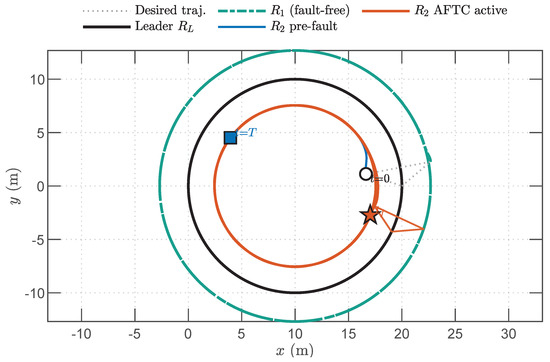
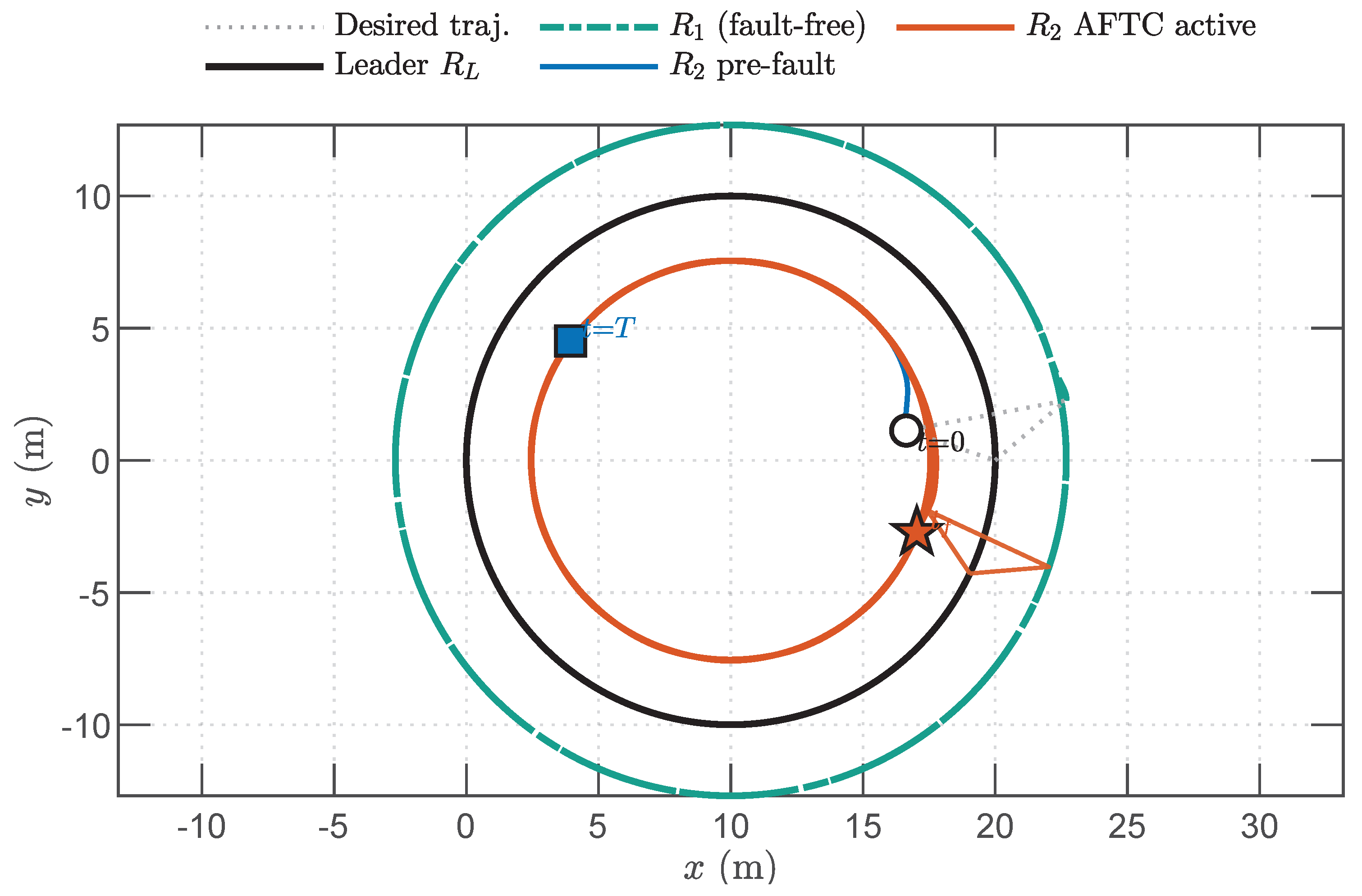
Figure 4 shows the two-dimensional convoy paths. $R_1$ maintains tight formation with the leader throughout the mission. $R_2$ deviates briefly at $t_f$ but rapidly reconverges to the circular formation under the AFTC law, preserving the triangular inter-vehicle geometry.

Figure 4. Two-dimensional formation trajectories over the simulation horizon (leader: black solid; $R_1$: teal dash-dot; $R_2$: blue before the fault, orange–red after).

4.4. Fault Estimation and State Recovery

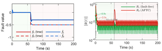
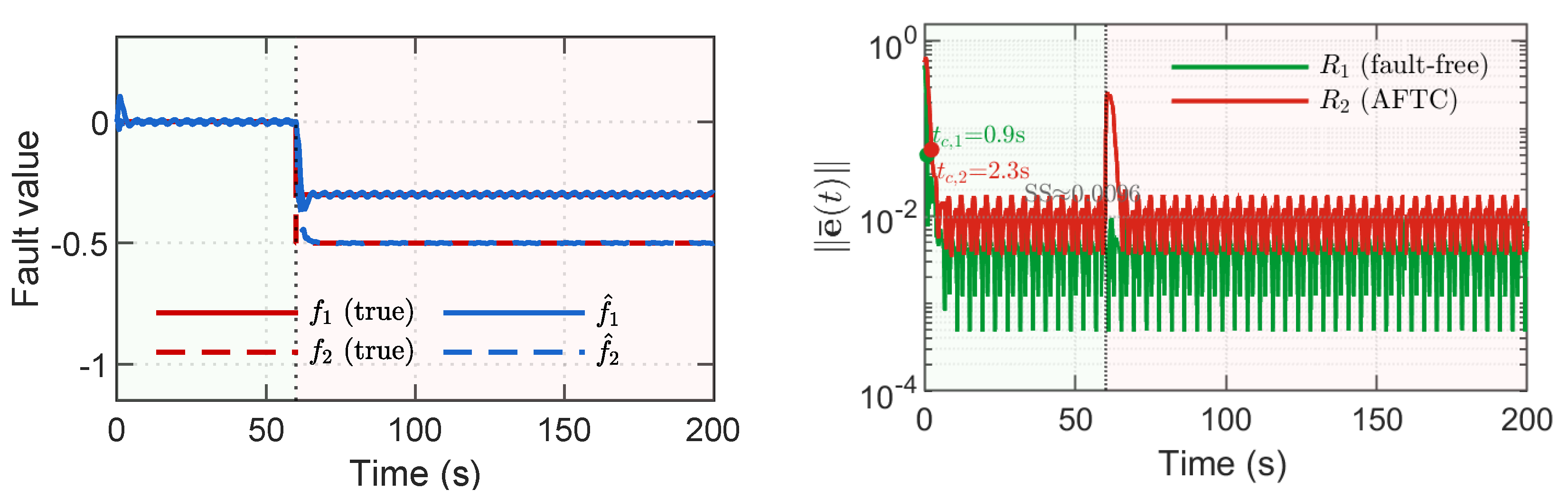
Figure 5 shows fault-estimate convergence and the evolution of the state-error norm $\parallel \mathbf{x}\left(t\right)\parallel$. Prior to $t_f$, the JEO maintains $\widehat{\mathbf{f}}\approx \mathbf{0}$. Upon fault injection, both fault components converge quickly to their true values (5% criterion; convergence time reported in Table 2). Although $\parallel \mathbf{x}\parallel$ for $R_2$ rises sharply at $t_f$, active compensation suppresses the transient within a few seconds of the fault-estimate convergence. Quantitative performance metrics are summarized in Table 2.

Figure 5. (Left) Fault estimates ${\widehat{f}}_1$, ${\widehat{f}}_2$ for $R_2$ (dashed) vs. true fault values (solid). (Right) State-error norms $\parallel \mathbf{x}\left(t\right)\parallel$ for $R_1$ (green) and $R_2$ (red).

Table 2. Quantitative performance metrics for the AFTC simulation.

Metric	${\mathit{R}}_1$ (Fault-Free)	${\mathit{R}}_2$ (AFTC)
Pre-fault SS-RMS of $\parallel \mathbf{x}\parallel$	≈0.005	≈0.010
Post-fault transient peak of $\parallel \mathbf{x}\parallel$	—	$0.262$
Fault-estimate convergence time $t_c$	—	≈3.2 s
Fault RMSE ($f_1$/$f_2$)	—	≈0.007/≈0.001
Post-fault SS-RMS of $\parallel \mathbf{x}\parallel$	≈0.005	≈0.011

4.5. Effect of Input Saturation

The stability and $H_{\infty }$ guarantees of Theorems 1 and 2 are established for the unsaturated linear control law $\overline{\mathbf{u}}=\mathbf{K}\widehat{\mathbf{x}}-\widehat{\mathbf{f}}$; the saturation limits $|v_i| \le 5.0$ m/s, $|{\omega }_i| \le 1.5$ rad/s are enforced in simulation as a hardware constraint. To limit the control effort along the closed-loop trajectory, the controller synthesis includes an auxiliary LMI that bounds the Lyapunov-weighted gain $\mathbf{K}{\mathbf{X}}_1{\mathbf{K}}^{\top }⪯K_{\max }^2\mathbf{I}$ with $K_{\max }=5$ (this coincides with a bound on ${\sigma }_{\max }\left(\mathbf{K}\right)$ only when ${\mathbf{X}}_1⪰\mathbf{I}$, so the realized gain may slightly exceed $K_{\max }$; here, $\parallel {\mathbf{K}}_1{\parallel }_2=4.75$ and $\parallel {\mathbf{K}}_2{\parallel }_2=6.56$). We therefore verify the effect of saturation a posteriori over the full run. The peak deviation commands are, for $R_1$, ${\max }_t\left|{\overline{v}}_i\right|=1.20$ m/s and ${\max }_t\left|{\overline{\omega }}_i\right|=0.86$ rad/s (limits never reached, $0.00\%$ of the horizon), and for $R_2$, ${\max }_t\left|{\overline{v}}_i\right|=0.48$ m/s and ${\max }_t\left|{\overline{\omega }}_i\right|=1.51$ rad/s. The only activation is a single brief transient on the $R_2$ angular-rate channel immediately after fault onset, where the command momentarily reaches $1.51$ rad/s ($0.4\%$ above the $1.5$ rad/s limit) for $0.01\%$ of the horizon. Away from this negligible transient, the closed loop coincides with the analyzed linear system and the $H_{\infty }$ guarantees apply; during the transient touch they hold in the anti-windup sense, so the reported recovery is a conservative (slightly slower) bound. This is stated explicitly as a limitation of the linear design.

4.6. Fault Transient Detail

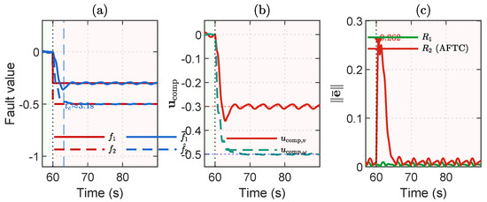
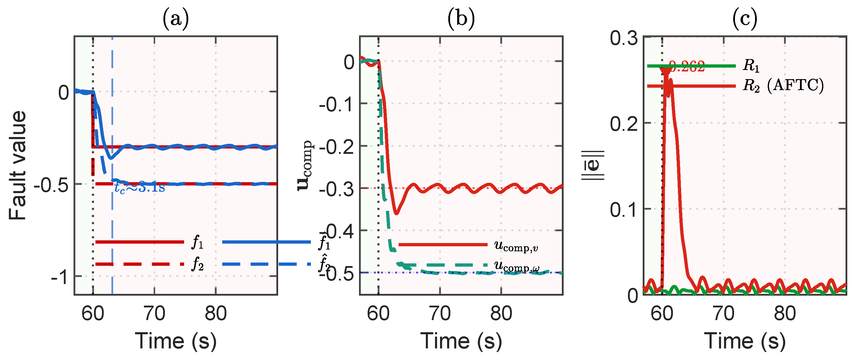
Figure 6 provides an enlarged view of $t\in [57,90]$ s. Panel (a) confirms fast fault-estimate convergence; panel (b) shows the compensation input tracking the true fault magnitudes; panel (c) shows $\parallel \mathbf{x}\parallel$ for $R_2$ peaking at $0.262$ and recovering to the pre-fault level within a few seconds, consistent with Theorem 2.

Figure 6. Enlarged fault transient ($t\in [57,90]$ s). (a) Fault-estimate convergence (5% band, dashed blue). (b) Compensation input ${\mathbf{u}}_{\mathrm{comp}}$, with the true fault magnitudes shown dotted. (c) State-error norm $\parallel \mathbf{x}\parallel$ for $R_2$ (red) vs. $R_1$ (green); the transient peak is marked ∇.

As Table 2 shows, the steady-state RMS error of $R_2$ after fault compensation is indistinguishable from that of fault-free $R_1$, validating both the compensation effectiveness of the proposed AFTC law and the $H_{\infty }$ performance bound established in Theorem 2.

5. Comparative Study

To place the proposed AFTC scheme in context, we compare it against three baseline controllers subject to the same physical fault scenario, initial conditions, and external disturbance used in Section 4.

Before presenting the baselines, we state a caveat that a reviewer of an earlier version rightly emphasized. The injected fault is a step additive matched actuator fault ($\mathbf{E}=\mathbf{B}$). For any fixed-gain state-feedback law $\mathbf{u}=\mathbf{K}\mathbf{x}$ the closed-loop steady state under a constant fault $\mathbf{f}$ is ${\mathbf{x}}_{ss}=-{(\mathbf{A}+\mathbf{B}\mathbf{K})}^{-1}\mathbf{B}\mathbf{f}$, which is nonzero whenever $\mathbf{f}\ne \mathbf{0}$; a permanent offset for the No-FTC and PFTC baselines is therefore structurally inevitable, not an artifact of poor tuning. The offset can be removed only by mechanisms that supply an equal-and-opposite constant control, of which the two canonical options are (a) integral action on the tracking error and (b) online fault estimation with feedforward cancellation, i.e., the proposed AFTC. We therefore add an integral-action baseline (I-H_∞) that, like AFTC, is capable of eliminating the offset, so that the comparison is not decided a priori by the absence of any offset-canceling mechanism. This isolates a genuine question: given that both AFTC and I-H_∞ remove the steady-state error, what does online fault reconstruction add?

5.1. Baseline Controllers

No-FTC: A standard $H_{\infty }$ state-feedback controller designed without any fault consideration. The gain ${\mathbf{K}}_{\mathrm{nf}}$ is obtained by solving the linear matrix inequality

$$\left[\begin{array}{ccc}\mathbf{A}\mathbf{X}+\mathbf{X}{\mathbf{A}}^{\top }+\mathbf{B}\mathbf{Y}+{\mathbf{Y}}^{\top }{\mathbf{B}}^{\top }& \mathbf{D}& \mathbf{X}\\ {\mathbf{D}}^{\top }& -{\gamma }_{\mathrm{nf}}^2& \mathbf{0}\\ \mathbf{X}& \mathbf{0}& -\mathbf{I}\end{array}\right]<0,$$

(35)

with ${\mathbf{K}}_{\mathrm{nf}}=\mathbf{Y}{\mathbf{X}}^{-1}$, ${\gamma }_{\mathrm{nf}}=3.0$. The disturbance channel contains $\mathbf{D}$ only; the fault channel $\mathbf{E}$ is absent from the design. Control law: $\mathbf{u}={\mathbf{K}}_{\mathrm{nf}}\mathbf{x}$ (no online fault estimation).

PFTC: A passive robust $H_{\infty }$ controller whose design treats the additive fault as an additional bounded disturbance with known entry direction [11]. The augmented disturbance matrix ${\mathbf{D}}_{\mathrm{aug}}=[\mathbf{D},\mathbf{E}]\in {\mathbb{R}}^{3\times 3}$ replaces $\mathbf{D}$ in (35), yielding gain ${\mathbf{K}}_{\mathrm{pf}}$ that simultaneously attenuates both w and $\mathbf{f}$ channels at the design stage, with ${\gamma }_{\mathrm{pf}}=3.0$. Control law: $\mathbf{u}={\mathbf{K}}_{\mathrm{pf}}\mathbf{x}$ (fixed gain, no online estimation).

I-H_∞ (integral-augmented): An offset-free robust baseline that augments the error state with its integral $\mathbf{q}={\int }_0^t\mathbf{x}\mathrm{d}\tau$. On the augmented plant with $\tilde{\mathbf{x}}={[{\mathbf{x}}^{\top },{\mathbf{q}}^{\top }]}^{\top }$, $\tilde{\mathbf{A}}=\left[\begin{array}{cc}\mathbf{A}& \mathbf{0}\\ \mathbf{I}& \mathbf{0}\end{array}\right]$, $\tilde{\mathbf{B}}={[{\mathbf{B}}^{\top },\mathbf{0}]}^{\top }$, $\tilde{\mathbf{D}}={[{\mathbf{D}}^{\top },\mathbf{0}]}^{\top }$, an integral-augmented state-feedback gain $\tilde{\mathbf{K}}=[{\mathbf{K}}_p,{\mathbf{K}}_i]$ is obtained by standard optimal state-feedback synthesis (a linear-quadratic regulator; equivalently an $H_{\infty }$ design) on the augmented plant, with the physical error $\mathbf{x}$ as the regulated variable. The control law is $\mathbf{u}={\mathbf{K}}_p\mathbf{x}+{\mathbf{K}}_i\mathbf{q}$ with conditional integration (the integrator is frozen while the command is saturated) to prevent windup. Because the integral state enforces ${\mathbf{x}}_{ss}=\mathbf{0}$ at equilibrium—the integrator supplies the constant control ${\mathbf{K}}_i{\mathbf{q}}_{ss}=-\mathbf{f}$ that cancels the matched fault—this baseline is offset-free for constant faults, exactly like AFTC, but uses no online fault estimate and no explicit fault model. It thus serves as the fair counterpart isolated in the caveat above.

The key structural distinction between the four strategies is summarized in Table 3.

Table 3. Summary of the four control strategies.

Strategy	Main Design Feature	Control law
No-FTC	No online fault estimation; only disturbance rejection	$\mathbf{u}={\mathbf{K}}_{\mathrm{nf}}\mathbf{x}$
PFTC	Fault treated as a bounded disturbance in the design stage	$\mathbf{u}={\mathbf{K}}_{\mathrm{pf}}\mathbf{x}$
I-H∞	Integral action on the error; offset-free but no fault model	$\mathbf{u}={\mathbf{K}}_p\mathbf{x}+{\mathbf{K}}_i\mathbf{q}$
AFTC (proposed)	Online fault reconstruction with feedforward compensation; offset-free and yields a fault estimate	$\mathbf{u}=\mathbf{K}\widehat{\mathbf{x}}-{\mathbf{B}}^{†}\mathbf{E}\widehat{\mathbf{f}}$

5.2. Results and Discussion

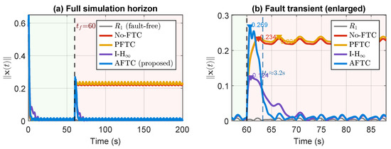
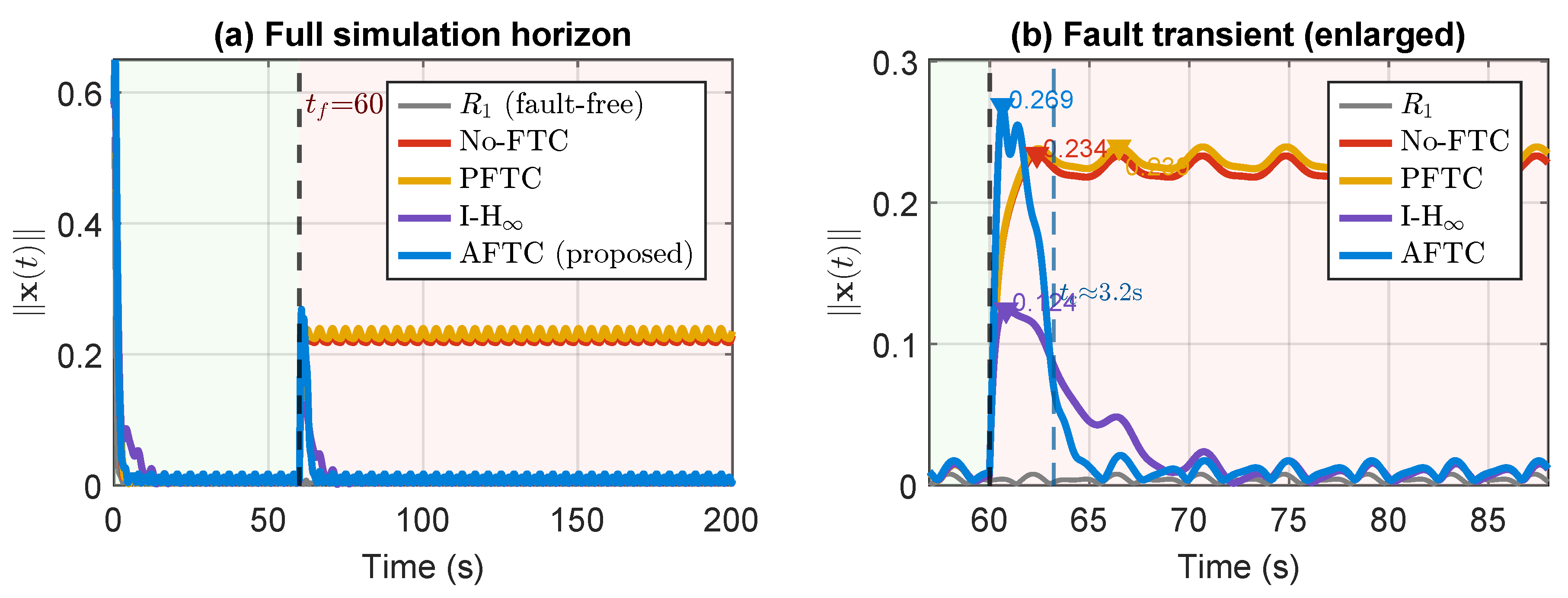
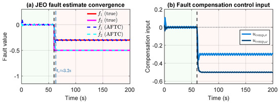
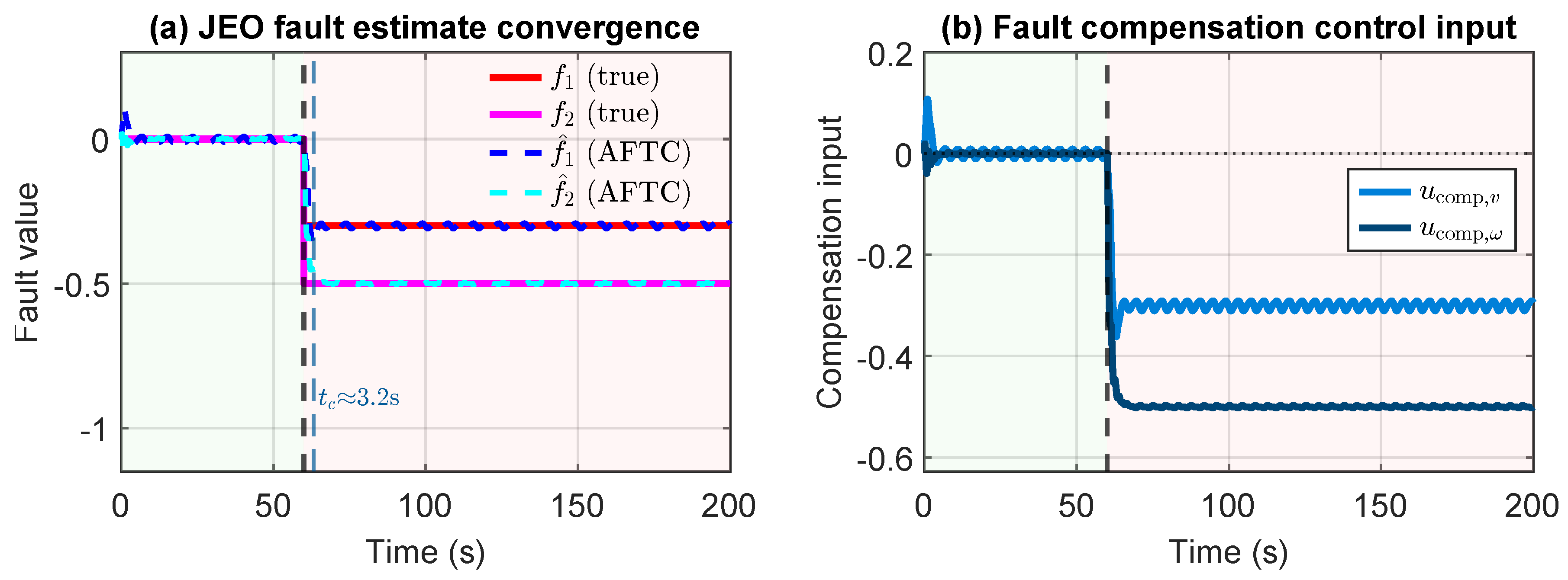
Figure 7 compares the state-error norm $\parallel \mathbf{x}\left(t\right)\parallel$ of follower $R_2$ under the four control strategies (No-FTC, PFTC, I-H_∞, and the proposed AFTC), while Figure 8 reports the internal signals of the proposed scheme that account for the observed behaviour. Quantitative metrics are collected in Table 4.

Figure 7. State-error norm $\parallel \mathbf{x}\left(t\right)\parallel$ of follower $R_2$ under the four control strategies, with $R_1$ as the fault-free reference. (a) Full simulation horizon. (b) Fault transient (enlarged).

Figure 8. Internal signals of the proposed AFTC scheme for follower $R_2$. (a) JEO fault-estimate convergence: estimates ${\widehat{f}}_1,{\widehat{f}}_2$ (dashed) vs. true fault values $f_1,f_2$ (solid). (b) Fault-compensation control input channels $u_{\mathrm{comp},v}$ and $u_{\mathrm{comp},\omega }$.

Table 4. Comparative performance metrics for $R_2$ under four control strategies; $R_1$ is shown as the fault-free reference.

Metric	${\mathit{R}}_1$	No-FTC	PFTC	I-H∞	AFTC
Pre-fault RMS of $\parallel \mathbf{x}\parallel$	0.0043	0.0089	0.0084	0.0087	0.0101
Post-fault transient peak	—	0.2341	0.2394	0.1242	0.2687
Fault-estimate convergence time	—	N/A	N/A	N/A	3.20 s
Recovery time to pre-fault band	—	no recovery	no recovery	7.5 s	3.6 s
Post-fault RMS of $\parallel \mathbf{x}\parallel$	0.0043	0.2237	0.2300	0.0093	0.0106

Pre-fault phase ($t<60$ s): All four controllers achieve comparable nominal performance with $\parallel \mathbf{x}\parallel$ converging to near-zero within ≈10 s. As reported in Table 4, the fixed-gain No-FTC and PFTC controllers attain a marginally lower pre-fault RMS than AFTC, whose slightly larger nominal error reflects the more conservative JEO-based Lyapunov structure used to jointly handle estimation and fault recovery; the I-H_∞ baseline is comparable to the fixed-gain controllers. All four remain at the same order as the fault-free $R_1$ level, so these nominal-performance differences are small in absolute terms.

Post-fault transient ($t\in [60,75]$ s): All strategies exhibit a spike at $t_f=60$ s. No-FTC and PFTC reach nearly identical peaks ($0.2341$ and $0.2394$, a difference of less than $2.3\%$), indicating that the passive robust gain provides negligible transient benefit when the fault magnitude and the disturbance channel are both bounded by the same $H_{\infty }$ design. The AFTC transient peak is slightly higher at $0.2687$: at the instant of fault onset the estimate $\widehat{\mathbf{f}}$ has not yet converged, so no compensation is applied during the first samples, and the larger AFTC gain ($\parallel {\mathbf{K}}_2{\parallel }_2=6.56$ vs. $5.42$ for No-FTC) momentarily amplifies the growing error. This transient penalty is short-lived: within $t_c=3.20$ s the fault estimate enters the $5\%$ error band (Figure 8), after which active cancellation returns $\parallel \mathbf{x}\parallel$ to the pre-fault band within $\approx 3.6$ s. The integral-action I-H_∞ baseline peaks at $0.1242$ and also returns to the pre-fault band, but only after its integrator has accumulated the required constant control, giving a recovery time of $7.5$ s. Comparing the two offset-free schemes on this transient is the fair test: AFTC cancels the matched fault by direct feedforward as soon as $\widehat{\mathbf{f}}$ converges, whereas I-H_∞ must integrate the error up, so the two recovery times $3.6$ s and $7.5$ s quantify the difference between feedforward cancellation and integral accumulation for this scenario.

Post-fault steady state ($t>120$ s): For No-FTC and PFTC, the step fault $\mathbf{f}$ acts as a permanent additive forcing term. Since the steady-state response satisfies ${\mathbf{x}}_{ss}=-{(\mathbf{A}+\mathbf{B}\mathbf{K})}^{-1}\mathbf{B}\mathbf{f}$, any fixed gain yields a nonzero offset whenever $\mathbf{f}\ne \mathbf{0}$. No-FTC settles at $\parallel {\mathbf{x}}_{ss}\parallel \approx 0.224$, representing a ≈22× degradation relative to the pre-fault level. PFTC settles at $\approx 0.230$—statistically indistinct from No-FTC—because $\mathbf{E}=\mathbf{B}$ and the $H_{\infty }$ gain-size trade-off under the same $K_{\max }$ bound cannot eliminate the permanent offset. Both offset-free schemes remove this error: AFTC’s online compensation term ${\mathbf{B}}^{†}\mathbf{E}\widehat{\mathbf{f}}$ directly cancels $\mathbf{B}\mathbf{f}$ once $\widehat{\mathbf{f}}\to \mathbf{f}$, restoring the post-fault steady-state RMS to $0.0106$, while I-H_∞ drives it to $0.0093$ via its integrator; both are practically identical to the pre-fault level and the fault-free $R_1$ baseline. The $21.1\times$ and $21.7\times$ steady-state improvements are therefore improvements over the fixed-gain No-FTC and PFTC baselines specifically and should be read as evidence that some offset-canceling mechanism is required, not as an advantage of AFTC over integral action, which the I-H_∞ column shows as also removing the offset. The distinctive value of AFTC over the equally offset-free I-H_∞ baseline is threefold and does not reduce to the steady-state number: (i) it produces an explicit estimate $\widehat{\mathbf{f}}$ of the fault, which I-H_∞ does not, making the fault directly available for detection, isolation, and health monitoring; (ii) it cancels the matched fault by feedforward rather than by charging an integrator, which for this scenario gives the recovery-time difference reported above and avoids integrator windup under the saturation of Section 4.5; and (iii) because the estimator tracks $\mathbf{f}\left(t\right)$ rather than only its constant part, it extends to time-varying faults, as examined in Section 6.

Fault-tolerance vs. nominal-performance trade-off: Table 4 makes explicit that active fault tolerance is not free: relative to the fixed-gain baselines, the proposed scheme incurs a marginally larger pre-fault tracking RMS and a slightly higher post-fault transient peak. Both penalties stem from the same design choice—the joint observer and the larger, more conservative compensating gain that make fault reconstruction and matched cancellation possible—and both are small: a nominal-RMS difference at the fault-free order, and a transient-peak difference of a few percent that persists only until $\widehat{\mathbf{f}}$ converges. In return, the scheme removes the otherwise permanent post-fault offset and supplies an explicit fault estimate. For the fault magnitudes and disturbance levels considered here, the trade-off is strongly favorable, since the transient and nominal cost is bounded and short-lived whereas the fixed-gain offset is permanent; where nominal tracking is at an absolute premium and faults are rare, a supervisory variant that engages the active compensation only after a fault is detected would recover the fixed-gain nominal performance while retaining fault tolerance.

6. Robustness Studies

The study in Section 4 uses a single scenario—one three-vehicle convoy, one follower fault, one step profile, one disturbance realization—which is adequate as a proof of concept but not to support broad robustness claims. This section therefore reports (i) a Monte Carlo campaign that randomizes the fault and the operating conditions, (ii) a variation of fault onset, magnitude, and type, (iii) a measurement-noise study, (iv) a model-mismatch study, and (v) a curvature-varying trajectory-change scenario (a serpentine/double-lane-change manoeuvre) in which the operating point drifts structurally so that the frozen linear-time-invariant design of Remark 1 is exercised outside its nominal point. All studies are produced by a common simulation pipeline, from which the aggregate numbers reported below and the exported figures are obtained. Unless stated otherwise, every trial reuses the observer/controller gains synthesized at the nominal operating point (no retuning), integrates the fault-augmented error model with the RK4 scheme and the saturation limits of Section 4, and reports four metrics for the faulty follower: the post-fault transient peak of $\parallel \mathbf{x}\parallel$, the recovery time to the pre-fault band, the post-fault steady-state RMS of $\parallel \mathbf{x}\parallel$, and the steady-state fault-reconstruction RMSE $\parallel \widehat{\mathbf{f}}-\mathbf{f}\parallel$.

6.1. Monte Carlo Campaign

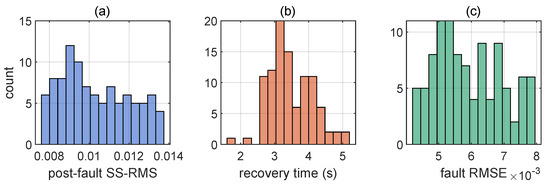
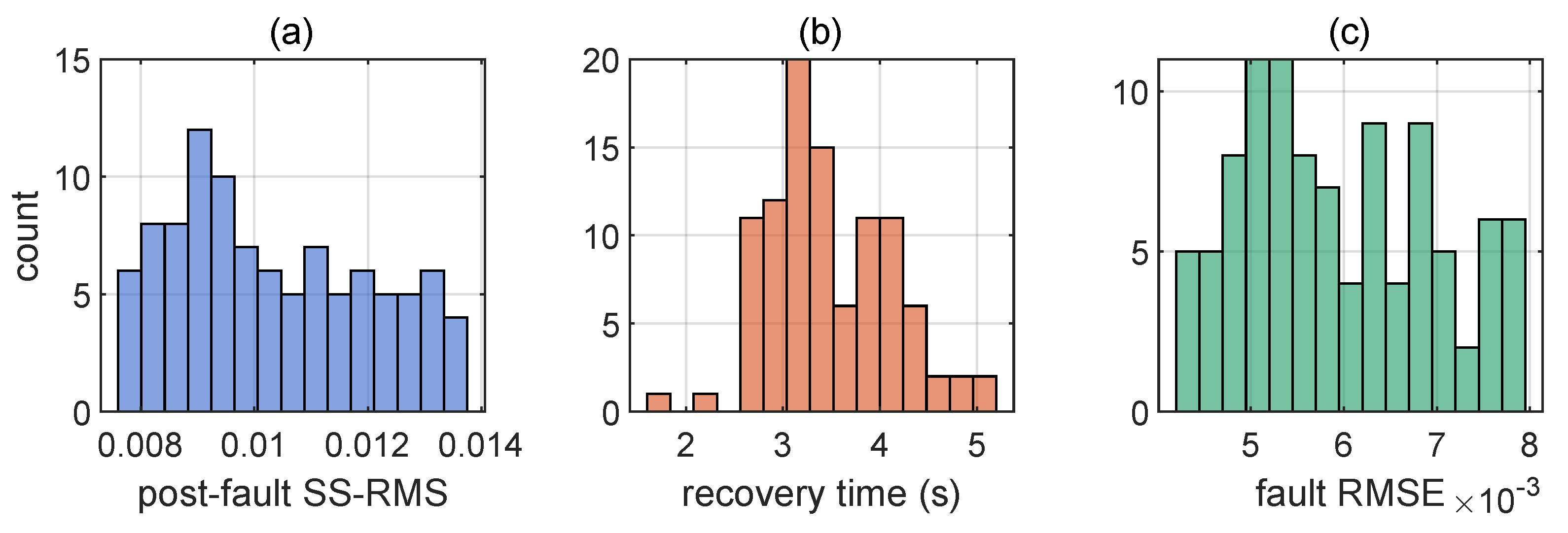
We run $N_{\mathrm{MC}}=100$ independent trials. In each trial, the fault onset $t_f$ is drawn uniformly from $[40,120]$ s, with each fault component from $[-0.6,0.6]$ (in m/s and rad/s, excluding a small dead-band around zero), the initial SBC error from a box around the nominal, and the disturbance as a random phase/amplitude realization of the same spectral class as in Section 4. A trial is counted successful when the post-fault steady-state RMS returns to within a factor $\kappa =3.0$ of the pre-fault band. Table 5 reports the mean ± standard deviation of each metric over the successful trials together with the success rate, and Figure 9 shows the distributions. The concentration of the steady-state RMS near the fault-free level indicates that offset elimination is not specific to a single nominal fault.

Table 5. Monte Carlo summary over $N_{\mathrm{MC}}=100$ randomized trials (mean ± std).

Metric	Value
Success rate (returns to pre-fault band)	100%
Post-fault transient peak of $\parallel \mathbf{x}\parallel$	0.1844
Recovery time to pre-fault band (s)	3.47
Post-fault steady-state RMS of $\parallel \mathbf{x}\parallel$	0.0103
Fault-reconstruction RMSE $\parallel \widehat{\mathbf{f}}-\mathbf{f}\parallel$	0.0059

Figure 9. Monte Carlo distributions over randomized trials: (a) post-fault steady-state RMS of $\parallel \mathbf{x}\parallel$; (b) recovery time; (c) fault-reconstruction RMSE.

6.2. Fault Onset, Magnitude, and Type

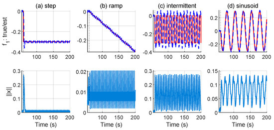
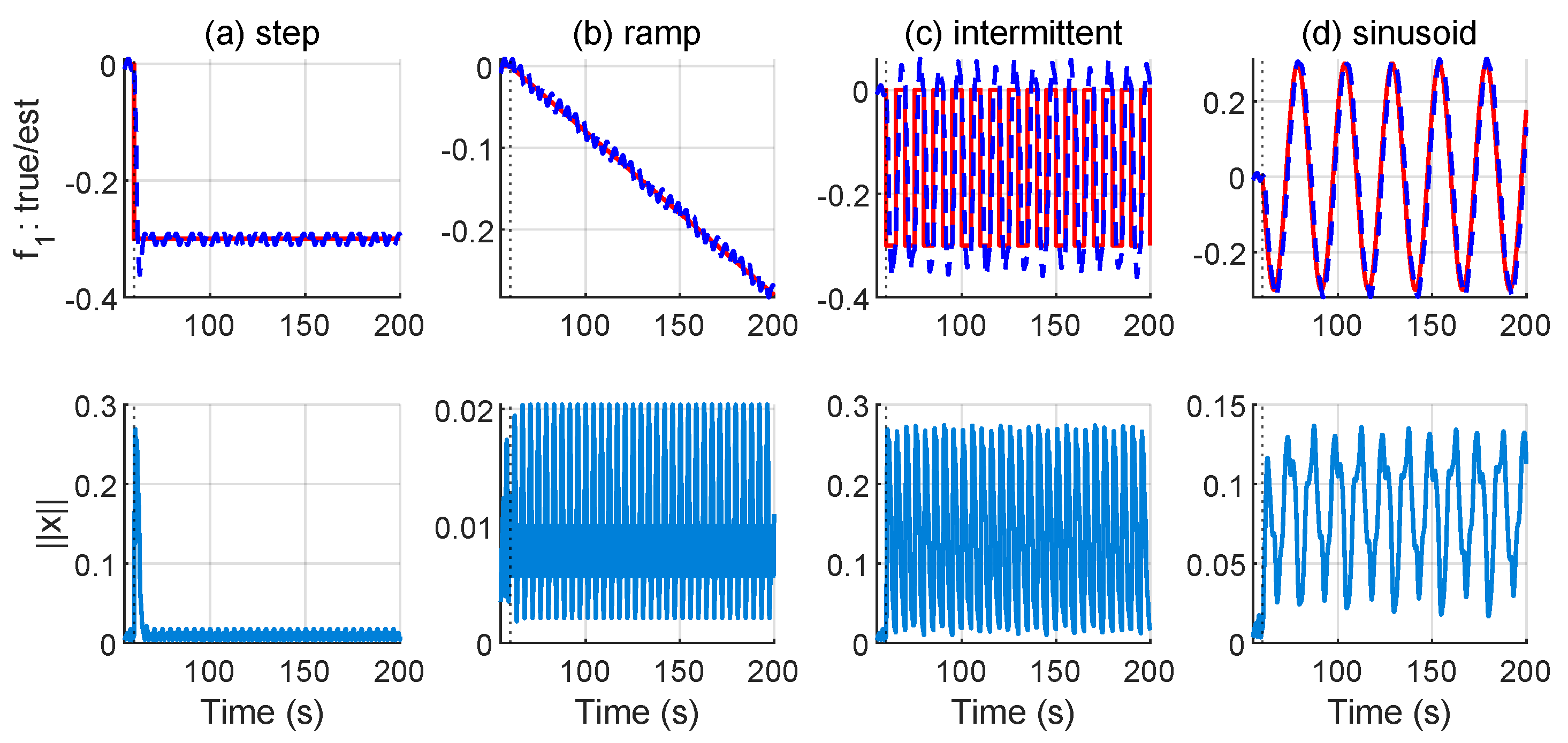
Holding the controller fixed, we vary the fault along three axes. First, the onset time is swept over $t_f\in \{45,60,80,100\}$ s to confirm that recovery is insensitive to when the fault strikes. Second, the magnitude is scaled over a range up to the point at which the saturation limits of Section 4 are reached, locating the largest fault the present (linear, saturated) design tolerates; the empirical threshold is $1.46$. Third, the fault type is changed from the nominal step to (a) a ramp $\mathbf{f}\left(t\right)=\mathbf{r}(t-t_f)$, (b) an intermittent (on/off) fault, and (c) a slowly varying sinusoid $\mathbf{f}\left(t\right)=\mathbf{a}\sin \left(\varpi t\right)$ consistent with Assumption 2. For the ramp and sinusoid the estimate tracks a moving target, so a bounded lag replaces exact convergence; the residual is governed by the observer attenuation ${\gamma }_{\mathrm{obs}}$, as anticipated in Remark 2. Figure 10 overlays the estimate and the error norm for the four fault types, and Table 6 lists the tracking lag and steady/bounded error for each.

Figure 10. Fault-type variation: true fault (solid), estimate (dashed), and error norm for step, ramp, intermittent, and sinusoidal faults under the same fixed controller.

Table 6. Effect of fault type on estimation and recovery (fixed controller).

Fault Type	Step	Ramp	Intermittent	Sinusoid
Fault-tracking error/lag	0.0061	0.0076	0.1377	0.0966
Post-fault RMS of $\parallel \mathbf{x}\parallel$	0.0106	0.0111	0.1588	0.0895

6.3. Measurement Noise

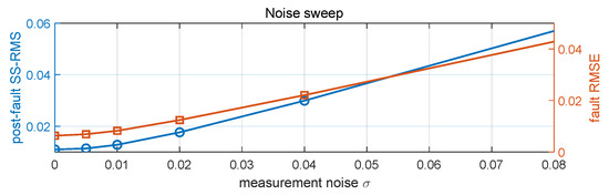
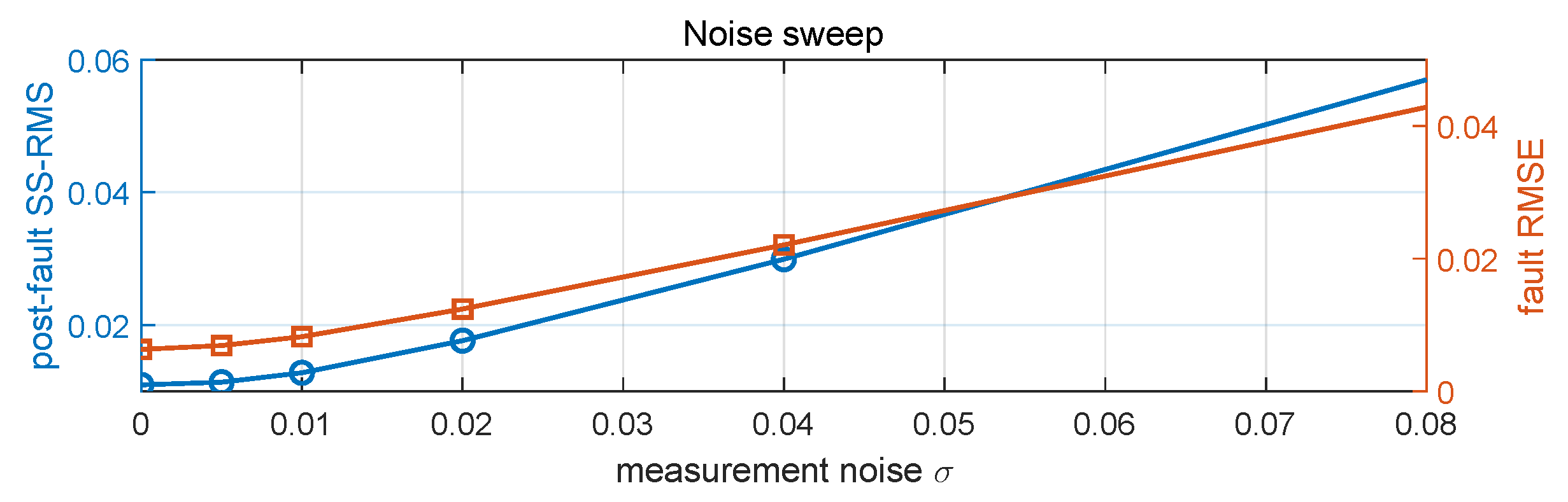
The nominal study assumes noise-free full-state measurement. Here, the measurement is corrupted as $\mathbf{y}=\mathbf{C}\mathbf{x}+\mathbf{n}$, with $\mathbf{n}$ zero-mean Gaussian noise whose per-channel standard deviation is swept over $\sigma \in \{0,0.005,0.01,0.02,0.04,0.08\}$. This study also substantiates Remark 3: the state channel of the joint observer filters $\mathbf{n}$ before it reaches the fault integrator, so the fault estimate degrades gracefully as $\sigma$ grows rather than tracking the raw noise. Figure 11 plots the steady-state RMS of $\parallel \mathbf{x}\parallel$ and the fault-reconstruction RMSE against $\sigma$; both increase smoothly, and up to $\sigma =0.02$ the post-fault RMS stays within $2\times$ the noise-free value.

Figure 11. Measurement-noise sweep: post-fault steady-state RMS of $\parallel \mathbf{x}\parallel$ (left axis) and fault-reconstruction RMSE (right axis) vs. the per-channel noise standard deviation $\sigma$.

6.4. Model Mismatch

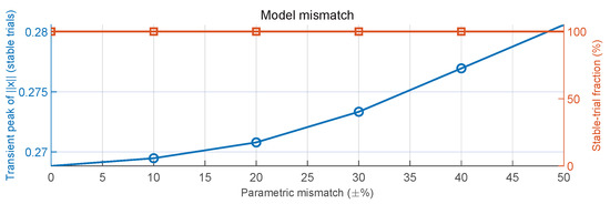
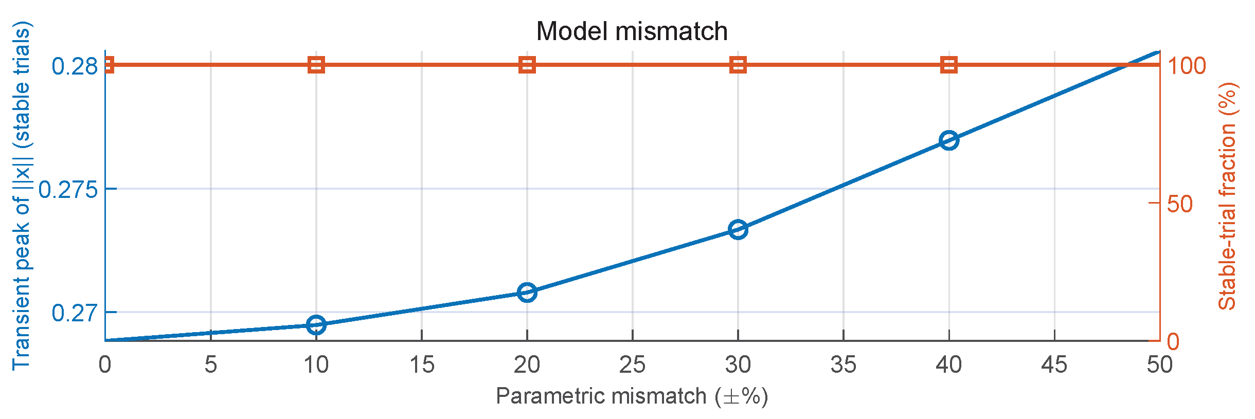
To probe sensitivity to modeling error, the gains $(\mathbf{L},\mathbf{\Gamma },\mathbf{K})$ are synthesized from the nominal model $({\mathbf{A}}_0,{\mathbf{B}}_0)$ but applied to a perturbed plant $(\mathbf{A},\mathbf{B})$ obtained by perturbing the physical parameters that enter the Jacobian of (6)—the desired separation $L_{li}^d$, the offset d, and the leader speed—by up to $\pm 50\%$. A useful structural property emerges here. Because the fault is matched ($\mathbf{E}=\mathbf{B}$) and the nominal compensation reduces to ${\mathbf{B}}_0^{†}{\mathbf{E}}_0\widehat{\mathbf{f}}=\widehat{\mathbf{f}}$, both the fault and its compensation enter the perturbed plant through the same input matrix $\mathbf{B}$, so the net residual forcing is $\mathbf{B}(\mathbf{f}-\widehat{\mathbf{f}})$, which vanishes once $\widehat{\mathbf{f}}\to \mathbf{f}$ regardless of how $\mathbf{B}$ differs from ${\mathbf{B}}_0$. Consequently, the post-fault steady-state offset is essentially invariant to parametric mismatch; the effect of mismatch appears instead in the transient and, for large perturbations, in the loss of closed-loop stability once the nominal gains no longer stabilize the perturbed plant. Figure 12 therefore reports the transient peak of $\parallel \mathbf{x}\parallel$ (over the trials that remain stable) together with the stable-trial fraction, both as functions of the mismatch level, and Table 7 summarizes the corresponding numbers. The design retains full stability up to $\pm 50\%$ mismatch, with the transient peak bounded by $0.2806$ over that range.

Figure 12. Model-mismatch study: transient peak of $\parallel \mathbf{x}\parallel$ (left axis) and stable-trial fraction (right axis) vs. parametric perturbation.

Table 7. Effect of parametric model mismatch (gains fixed at nominal).

Mismatch Level	0%	±20%	±50%
Post-fault RMS of $\parallel \mathbf{x}\parallel$ (mean)	0.0106	0.0106	0.0106
Fault-reconstruction RMSE (mean)	0.0061	0.0061	0.0062
Stable-trial fraction	100%	100%	100%

6.5. Trajectory Change

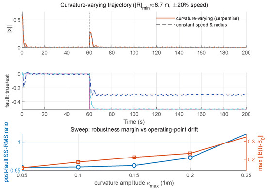
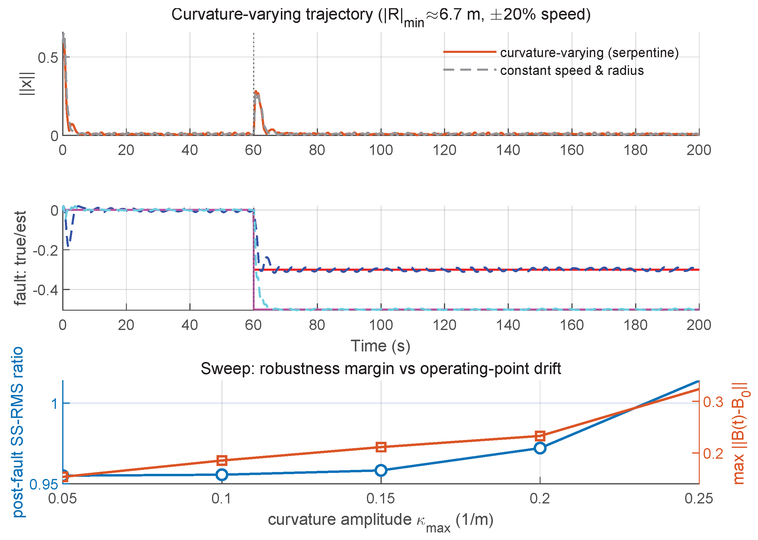
Finally, to exercise the genuinely time-varying regime deferred in Remark 1 under a geometrically more demanding reference than the nominal circle, the leader executes a curvature-varying serpentine (double-lane-change) manoeuvre: its linear speed is modulated by $\pm 20\%$ (period 80 s) while its turn rate is driven so that the path curvature $\kappa \left(t\right)={\omega }_l\left(t\right)/v_l\left(t\right)$ oscillates about zero, $\kappa \left(t\right)={\kappa }_{\max }\sin (2\pi t/T_{\kappa })$ with ${\kappa }_{\max }=0.15{\mathrm{m}}^{-1}$ and $T_{\kappa }=40$ s. The leader therefore alternates left and right turns down to a minimum instantaneous radius ${\left|R\right|}_{\min }=1/{\kappa }_{\max }\approx 6.7$ m, rather than following a fixed circle at varying speed. Because both the desired SBC state ${\mathit{\chi }}_i^d\left(t\right)$ and the nominal input ${\mathbf{u}}_i^d\left(t\right)$ now change along the path, the operating point—and hence the true Jacobians $\mathbf{A}\left(t\right),\mathbf{B}\left(t\right)$ of the error model—drifts structurally (not merely in scale), while the controller and observer keep the fixed gains computed at the nominal point (no gain scheduling). This is the frozen-time application of the constant design to a genuinely LTV plant.

To confirm that the induced perturbation is non-trivial, we track the drift of the input Jacobian relative to its nominal value ${\mathbf{B}}_0$ along the run: the nominal heading offset ${\phi }_i^d$ excursion reaches $\max |\Delta {\phi }_i^d|=13.9^{°}$ and the input-matrix drift reaches $\max \parallel \mathbf{B}\left(t\right)-{\mathbf{B}}_0{\parallel }_2=0.211$ (a relative change of $21\%$), i.e., the frozen gains are applied to a plant whose control-input geometry departs materially from the design point—in contrast to the constant-speed circle, where this drift is identically zero. Figure 13 reports the error norm and the fault estimate across the maneuver with the same fault injected mid-run. Despite this $21\%$ structural operating-point drift, the closed loop remains stable and bounded and the fault estimate still tracks the injected fault: the post-fault RMS of $\parallel \mathbf{x}\parallel$ is, if anything, marginally lower than for the constant-speed/constant-radius baseline (a ratio of $0.96$). This is expected—the serpentine curvature oscillates about zero, so the time-averaged manoeuvre is no more aggressive than the fixed circle, and the point of the test is not that the ratio exceeds unity but that a genuinely time-varying plant with a $21\%$ Jacobian excursion is handled by the frozen-LTI gains with no degradation. To map the robustness margin against the severity of the maneuver, we sweep the curvature amplitude ${\kappa }_{\max }\in [0.05,0.25]{\mathrm{m}}^{-1}$ (bottom panel of Figure 13), which drives the input-matrix drift from $0.15$ up to $0.32$ (heading excursion from $10.2°$ to $27.8°$): the post-fault RMS ratio rises smoothly and monotonically with this drift—from $0.96$ at ${\kappa }_{\max }=0.05$ to $1.01$ at ${\kappa }_{\max }=0.25$—with no abrupt loss of stability over the tested range, exactly the graceful degradation predicted by frozen-time/slowly-varying arguments. Larger or faster excursions than those tested would call for the parameter-dependent (LPV/gain-scheduled) extension noted in Section 7.

Figure 13. Curvature-varying trajectory-change scenario (AFTC gains held fixed at their nominal-point values). (Top): error norm $\parallel \mathbf{x}\parallel$. (Middle): true and estimated fault components. (Bottom): post-fault RMS ratio and input-matrix drift $\parallel \mathbf{B}\left(t\right)-{\mathbf{B}}_0\parallel$ vs. curvature amplitude ${\kappa }_{\max }$.

• Applicability to general trajectories: The scenario above already exercises a curvature-varying reference—the effect most relevant in practice is the resulting drift of the operating point—and the same reasoning covers more general references. For any sufficiently smooth desired trajectory, the linearization applies pointwise: expanding about the (now time-varying) operating point yields the LTV error model $\dot{\mathbf{x}}=\mathbf{A}\left(t\right)\mathbf{x}+\mathbf{B}\left(t\right)\overline{\mathbf{u}}+\dots$, and the gains synthesized at the nominal point act as a frozen-time controller on that model. The serpentine study above shows this frozen design keeps a useful margin for the combined speed-and-curvature excursions typical of convoy lane-change maneuvers, and the curvature sweep makes its graceful degradation as the operating-point drift grows explicit—consistent with standard frozen-time/slowly-varying arguments: the design is expected to remain effective as long as the operating point varies slowly relative to the closed-loop bandwidth. For aggressive or persistently time-varying references—curvature beyond the tested range, large speed swings, or trajectories that never settle—this margin is no longer guaranteed, and the appropriate methodology is to schedule the observer and controller gains along the trajectory (a linear-parameter-varying/parameter-dependent-Lyapunov design), identified as the natural extension in Section 7. A full LTV/LPV synthesis and its experimental validation are beyond the scope of the present proof-of-concept study.

7. Conclusions

This paper presented an observer-based active fault-tolerant control scheme for leader–follower formations of differential-drive unmanned ground vehicles operating under the Separation-Bearing Control representation. Rather than a new estimation or control methodology, the contribution is the adaptation and integration of established $H_{\infty }$ observer and active-compensation tools to the geometrically coupled Separation-Bearing Control setting, in which a single matched actuator fault corrupts all three formation states at once. The nonlinear Separation-Bearing Control kinematics were linearized about the rigid-formation operating point; for a constant-speed reference, this operating point is stationary, so the fault-augmented error model is linear-time-invariant. A joint estimation observer and a state-feedback controller were then designed; the combined linear closed loop was certified asymptotically stable with a prescribed disturbance-attenuation bound, which by the indirect method establishes local asymptotic stability of the corresponding equilibrium of the nonlinear formation.

Simulations of a three-vehicle circular convoy confirmed rapid fault-estimate convergence and effective formation-error recovery following a step actuator fault, consistent with the theoretical guarantees established in the design section. A comparative study against non-fault-tolerant, passive, and integral-action baselines showed that fixed-gain approaches leave a structurally inevitable steady-state offset, that both the proposed scheme and an integral-action controller remove it, and that the distinctive value of the proposed scheme over integral action is the explicit fault reconstruction it provides—useful for diagnosis and for feedforward cancellation of time-varying faults. Monte Carlo, fault-variation, measurement-noise, model-mismatch, and trajectory-change studies further indicated that this behavior is not specific to the single nominal scenario.

Several limitations delimit the present contribution and motivate future work. First, the design rests on the matched additive-fault assumption $\mathbf{E}=\mathbf{B}$; unmatched actuator faults and sensor faults, for which $\mathbf{E}\ne \mathbf{B}$, are attenuated but not exactly canceled by the current compensator, and extending exact reconstruction to these cases (e.g., via input augmentation or unknown-input observers) is an open problem. Second, the stability and $H_{\infty }$ certificates are derived for the unsaturated law; a formal treatment of input saturation through anti-windup or explicit constraint-handling (e.g., model-predictive) synthesis would remove the a posteriori saturation check used here. Third, the certificates hold for the linear model obtained by linearizing about the operating point and are therefore local in the nonlinear state space and time-invariant only for a constant-speed reference; a global result for the full nonlinear Separation-Bearing Control kinematics via a nonlinear Lyapunov construction, a parameter-dependent (or gain-scheduled) extension for genuinely time-varying references, and experimental validation on a physical UGV platform all remain to be established.

References

- Sun, L.; Yang, Y.; Duan, Q.; Shi, Y.; Lyu, C.; Chang, Y.-C.; Lin, C.-T.; Shen, Y. Multi-agent coordination across diverse applications: A survey. arXiv 2025, arXiv:2502.14743. [Google Scholar]
- Yang, R.; Liu, L.; Feng, G. An overview of recent advances in distributed coordination of multi-agent systems. Unmanned Syst. 2022, 10, 307–325. [Google Scholar] [CrossRef] [Scilit]
- Liu, W.; Wang, X.; Li, S. Formation control for leader–follower wheeled mobile robots based on embedded control technique. IEEE Trans. Control Syst. Technol. 2023, 31, 265–280. [Google Scholar] [CrossRef] [Scilit]
- Chen, Q.; Wang, Y.; Jin, Y.; Wang, T.; Nie, X.; Yan, T. A survey of an intelligent multi-agent formation control. Appl. Sci. 2023, 13, 5934. [Google Scholar] [CrossRef] [Scilit]
- Wen, B.; Huang, J. Leader-following formation tracking control of nonholonomic mobile robots considering collision avoidance: A system transformation approach. Appl. Sci. 2022, 12, 12579. [Google Scholar] [CrossRef] [Scilit]
- Wang, J.; Peng, Y.; Wen, S.; Wang, H.; Wan, Y. Formation control for multiple nonholonomic wheeled mobile robots based on integrated sliding mode controller and force function. Proc. Inst. Mech. Eng. I J. Syst. Control Eng. 2024, 238, 01423312241291093. [Google Scholar]
- Lin, J.; Miao, Z.; Zhong, H.; Peng, W.; Wang, Y.; Fierro, R. Adaptive image-based leader–follower formation control of mobile robots with visibility constraints. IEEE Trans. Ind. Electron. 2021, 68, 6010–6019. [Google Scholar] [CrossRef] [Scilit]
- Li, W.; Zhang, H.; Cai, Y.; Wang, Y. Fully distributed formation control of general linear multiagent systems using a novel mixed self- and event-triggered strategy. IEEE Trans. Syst. Man. Cybern. Syst. 2022, 52, 5736–5745. [Google Scholar] [CrossRef] [Scilit]
- Nuño, E.; Ortega, R.; Basañez, L. Global consensus-based formation control of perturbed nonholonomic mobile robots with time-varying delays. Automatica 2022, 141, 110294. [Google Scholar]
- Loría, A.; Nuño, E.; Panteley, E. Leader-follower consensus formation control of differential-drive nonholonomic vehicles with time-varying delays. In Proceedings of the 29th Mediterranean Conference on Control and Automation (MED), Puglia, Italy, 22–25 June 2021; pp. 1240–1245. [Google Scholar]
- Abbaspour, A.; Mokhtari, S.; Sargolzaei, A.; Yen, K.K. A survey on active fault-tolerant control systems. Electronics 2020, 9, 1513. [Google Scholar] [CrossRef] [Scilit]
- Ling, X.; Xu, H.; Zhu, F. Active compensation fault-tolerant control for uncertain systems with both actuator and sensor faults. Sensors 2026, 26, 267. [Google Scholar] [CrossRef] [Scilit] [PubMed]
- Li, Y.; Liu, Y.; Zhu, L.; Guo, Y. Fault-tolerant formation control of heterogeneous multi-agent systems with unknown inputs and external disturbances. Sci. Rep. 2025, 15, 20773. [Google Scholar] [CrossRef] [Scilit] [PubMed]
- Xu, L.; Tian, B.; Wang, C.; Lu, J.; Wang, D.; Li, Z.; Zong, Q. Fixed-time disturbance observer-based MPC robust trajectory tracking control of quadrotor. IEEE/ASME Trans. Mechatron. 2025, 30, 4272–4282. [Google Scholar] [CrossRef] [Scilit]
- Flores-Resendiz, J.B.; Aranda-Bricaire, E.; González-Sierra, J.; Escaño, J. Trajectory tracking nonlinear H∞ controller for wheeled mobile robots with disturbances observer. ISA Trans. 2023, 137, 503–514. [Google Scholar]
- Wang, X.; Tan, C.P.; Zhou, D. A novel sliding mode observer for state and fault estimation in systems not satisfying matching and minimum phase conditions. Automatica 2017, 79, 290–295. [Google Scholar] [CrossRef] [Scilit]
- Sader, M.; Chen, Z.; Liu, Z.; Deng, C. Distributed robust fault-tolerant consensus control for a class of nonlinear multi-agent systems with intermittent communications. Appl. Math. Comput. 2021, 403, 126166. [Google Scholar] [CrossRef] [Scilit]
- Cui, B.; Mao, L.; Xia, Y.; Ma, T.; Gao, H. Fixed-time fault-tolerant consensus control for high-order nonlinear multiagent systems under directed topology. IEEE Trans. Control Netw. Syst. 2024, 11, 197–209. [Google Scholar] [CrossRef] [Scilit]
- Yang, Z.; Li, M.; Yu, Z.; Cheng, Y.; Xu, G.; Zhang, Y. Fault detection and fault-tolerant cooperative control of multi-UAVs under actuator faults, sensor faults, and wind disturbances. Drones 2023, 7, 503. [Google Scholar] [CrossRef] [Scilit]
- Zheng, Z.; Tong, S.; Wang, E.; Zhu, Y.; Shao, J. Robust consensus tracking control for multi-unmanned-aerial-vehicle (UAV) system subjected to measurement noise and external disturbance. Drones 2025, 9, 61. [Google Scholar] [CrossRef] [Scilit]
- Shahab, M.; Nasir, A.; Alyazidi, N.M. Formation control of wheeled mobile robots with fault-tolerance capabilities. Robotics 2025, 14, 59. [Google Scholar] [CrossRef] [Scilit]
- Jouili, A.; Boussaid, B.; Zouinkhi, A.; Abdelkrim, M.N. Fault detection of multi-wheeled robot consensus based on EKF. Actuators 2024, 13, 253. [Google Scholar] [CrossRef] [Scilit]
- Zhao, Y.; Li, D.; Li, Y.; Gong, D.; Chen, J.; Song, S.; Zhu, M. Data-driven fully distributed fault-tolerant consensus control for nonlinear multi-agent systems: An observer-based approach. Mathematics 2025, 13, 3582. [Google Scholar] [CrossRef] [Scilit]
- Luo, J.; Li, K.; Yang, H.; Yang, J. Comparison on inverse-free method and pseudoinverse method for fault-tolerant planning of redundant manipulator. IEEE Access 2020, 8, 178796–178804. [Google Scholar] [CrossRef] [Scilit]
- Liu, Z.-Q.; Ge, X.; Xie, H.; Han, Q.-L.; Zheng, J.; Wang, Y.-L. Secure leader–follower formation control of networked mobile robots under replay attacks. IEEE Trans. Ind. Inform. 2024, 20, 4149–4159. [Google Scholar] [CrossRef] [Scilit]
- Ye, H.; Song, Y. A separation principle for the prescribed-time stabilization of a class of nonlinear systems. Automatica 2025, 171, 111983. [Google Scholar] [CrossRef] [Scilit]
- Li, L.; Kuang, C.; Xia, Y.; Qiang, J. Formation control of nonholonomic mobile robots with inaccurate global positions and velocities. Int. J. Robust Nonlinear Control 2022, 32, 9776–9790. [Google Scholar] [CrossRef] [Scilit]
- Saradagi, A.; Muralidharan, V.; Krishnan, V.; Menta, S.; Mahindrakar, A.D. Formation control and trajectory tracking of nonholonomic mobile robots. IEEE Trans. Control Syst. Technol. 2018, 26, 2250–2258. [Google Scholar] [CrossRef] [Scilit]
- Wang, H.; Wang, Q.; Zhang, H.; Han, J. H∞ observer for vehicle steering system with uncertain parameters and actuator fault. Actuators 2022, 11, 43. [Google Scholar] [CrossRef] [Scilit]
- Mohite, S.; Alma, M.; Zemouche, A. Estimating faults/attacks using a fast adaptive unknown input observer: An enhanced LMI approach. IEEE Control Syst. Lett. 2024, 8, 448–453. [Google Scholar]
Disclaimer/Publisher’s Note: The statements, opinions and data contained in all publications are solely those of the individual author(s) and contributor(s) and not of MDPI and/or the editor(s). MDPI and/or the editor(s) disclaim responsibility for any injury to people or property resulting from any ideas, methods, instructions or products referred to in the content. |
© 2026 by the authors. Licensee MDPI, Basel, Switzerland. This article is an open access article distributed under the terms and conditions of the Creative Commons Attribution (CC BY) license.