


Highlights
What are the main findings?
- Segmented RPM scheduling alone reduces the synchronization error by 98.9% (from 1.192 s to 0.013 s) while keeping the original path geometry unchanged.
- Phase-circle retention alone shortens the total path length by 30.9% (from 37.75 km to 26.10 km) and achieves a 99.4% error reduction.
What is the implication of the main finding?
- Phase-circle retention provides coarse flight-time adjustment through path shortening, whereas segmented RPM scheduling offers fine timing correction; their joint optimization achieves sub-millisecond synchronization s.
- Wind-aware flight-time prediction is essential: ignoring wind introduces a flight-time bias of 28–31 s and alters the optimal retention ratios and RPM schedules.
Abstract
Cooperative UAV missions often require multiple vehicles to reach a target area at nearly the same time. For small-turbofan UAVs flying along recorded routes, this timing task is affected by path-length differences, spatially varying wind, and phase-circle segments kept for waiting or coordination. Under these conditions, using only a fixed cruise setting often leaves limited room for arrival-time adjustment. This paper develops a wind-aware synchronized-arrival optimization method for small-turbofan UAVs based on segmented RPM scheduling and phase-circle retention. The method combines local wind projection along the path, an empirical RPM-to-airspeed model, and discrete flight-time integration, and it evaluates three timing-adjustment modes: fixed-alpha segmented RPM optimization, fixed-RPM phase-circle retention optimization, and their joint optimization. The method is tested on the recorded trajectories of UAV 13 and UAV 14, using a reconstructed wind field obtained from multi-UAV flight data. In the wind-aware constant-RPM baseline, both UAVs keep the full phase-circle segments and fly at 6500 rpm, which gives a predicted synchronization error of s. Segmented RPM optimization reduces the error to s. Phase-circle retention optimization reduces it to s and shortens the total path length from 37,752.3 m to 26,103.4 m. The joint optimization gives the best result, with a synchronization error of s and a total path length of 26,094.4 m. A no-wind ablation study also shows that ignoring wind leads to a total flight-time bias of about 29–31 s. These results indicate that phase-circle retention is effective for coarse flight-time adjustment through path shortening, whereas segmented RPM scheduling is better suited to fine timing correction. Using the two together improves synchronized-arrival prediction and adjustment for recorded UAV paths in wind.
1. Introduction
Cooperative unmanned aerial vehicle (UAV) missions require coordination in both space and time. In reconnaissance, surveillance, communication relay, disaster monitoring, and emergency delivery, multiple vehicles may need to reach a target region within a limited time window. If this timing requirement is not met, sensing coverage, task handover, formation reconfiguration, and follow-on actions may all be affected. Synchronized arrival has therefore become an important problem in multi-UAV planning and coordination, especially when trajectory design and timing control must be considered together [1,2,3,4]. Recent work on UAV path planning, swarm coordination, and evolutionary optimization likewise shows continued interest in cooperative trajectory generation under temporal and mission-related constraints [5,6,7].
For fixed-wing UAVs, arrival time depends on both path geometry and the speed profile along the route. The path geometry must also satisfy the vehicle’s kinematic constraints, such as minimum turning radius, which are often addressed using Dubins path formulations [8]. When vehicles depart from different locations or follow routes with different shapes, their travel times can diverge because of differences in path length, turning structure, and local heading. Under simplified assumptions, this mismatch can be reduced by changing route length, assigning different cruise speeds, or shifting departure times [9,10]. In low-altitude operations, however, wind makes the problem harder. The relation between airspeed and ground speed changes with the local wind field, and the along-track wind component varies with position, altitude, and path direction. As a result, two UAVs flying under the same nominal speed or propulsion command may still accumulate different travel times along different routes. Studies on non-uniform wind fields have also reported their effects on guidance accuracy, path following, energy consumption, and trajectory execution [11]. When communication limits, energy constraints, kinematic feasibility, and formation requirements are also present, synchronized-arrival planning depends on a flight-time model that reflects both local wind variation and actual path geometry.
Existing timing-adjustment methods usually emphasize either path modification or speed regulation. Path-based methods alter the route to satisfy temporal requirements, for example by constructing equal-length paths, inserting loiter segments, or adding circular holding patterns to absorb timing differences. Although intuitive, these treatments may add substantial distance and reduce path efficiency when large corrections are needed. In formation flight, obstacle-rich environments, and complex three-dimensional missions, geometric adjustment is also coupled with feasibility and coordination constraints [12]. This is one reason why intelligent optimization methods, including particle swarm optimization, genetic algorithms, and reinforcement-learning-assisted metaheuristics, have been widely explored in UAV and multi-UAV path planning [13,14]. Speed-regulation methods preserve the geometry and adjust the speed profile along it, which avoids extra detours. However, many formulations still optimize an ideal ground-speed or airspeed profile directly, while the mapping from that profile to propulsion-feasible commands is simplified and the wind contribution along the actual route is not modeled explicitly. This can create a mismatch between predicted arrival time and what the vehicle can achieve in practice.
For small-turbofan fixed-wing UAVs, engine rotational speed, expressed in revolutions per minute (RPM), is a practical variable for timing adjustment. RPM is usually available in flight logs and reflects engine operating condition more directly than an abstract cruise-speed command. Recent studies on turbojet, micro-aero engines, and propulsion-system modeling show that measured data can support practical identification of thrust, shaft speed, and engine dynamics [15,16,17]. Related work on UAV propulsion and rotor-speed modeling also highlights the usefulness of RPM-related variables in performance characterization and control-oriented analysis [18,19]. At the same time, recorded UAV routes may contain phase-circle or loiter-like segments introduced for waiting, formation coordination, timing adjustment, or task synchronization. Keeping these segments in full increases total distance and mission duration, whereas removing them without additional timing compensation may violate the synchronized-arrival requirement. This creates a coupled problem in which propulsion scheduling and local path adjustment must be considered together.
This paper proposes a wind-aware synchronized-arrival optimization method for cooperative small-turbofan UAVs flying along recorded paths. The method takes recorded trajectories, a common target position, a reconstructed wind field, and an empirical RPM-to-airspeed model as inputs. Along each path segment, the local wind is interpolated and projected onto the path direction to obtain the along-track wind component. The corresponding airspeed is then estimated from the RPM command, and ground speed and flight time are computed through discrete integration. On this basis, segmented RPM scheduling and phase-circle retention are studied both separately and jointly.
Unlike MPC-based synchronized control methods or cooperative path-planning approaches that focus on online feedback control, receding-horizon replanning, or global trajectory redesign, this study addresses a complementary mission-level problem: wind-aware arrival-time coordination along recorded or preassigned UAV trajectories. The proposed framework preserves the main recorded path structure while adjusting arrival time through segmented RPM scheduling and selective phase-circle retention under a reconstructed wind field.
The experiments use recorded flight data from 16 UAVs for wind-field reconstruction and RPM-to-airspeed model identification. UAV 13 and UAV 14 are selected as the synchronized-arrival pair because both trajectories contain clear phase-circle segments before the common target. Five cases are considered: a wind-aware constant-RPM baseline, fixed-alpha segmented RPM optimization, fixed-RPM phase-circle retention optimization, joint phase-circle retention and segmented RPM optimization, and a no-wind ablation study. This setup allows the individual and combined effects of wind modeling, RPM scheduling, and retained phase-circle geometry to be evaluated within the same recorded-path framework.
The main contributions of this paper are summarized as follows:
- A wind-aware flight-time prediction method is developed for recorded UAV paths using along-track wind projection, an empirical RPM-to-airspeed model, and discrete flight-time integration.
- A synchronized-arrival optimization framework is formulated for small-turbofan UAVs with RPM constraints and redundant phase-circle segments, including fixed-alpha segmented RPM optimization, fixed-RPM phase-circle retention optimization, and joint optimization.
- Recorded multi-UAV flight data and a no-wind ablation study are used to evaluate the effects of wind-aware prediction, segmented RPM scheduling, and phase-circle retention on synchronized-arrival performance.
2. Methodology
This study considers synchronized arrival for small-turbofan UAVs flying along given paths under wind. The paths are taken from recorded trajectories and are used together with a common target position, a reconstructed wind field, and an empirical RPM-to-airspeed relation. Along each trajectory, the local wind vector is interpolated from the reconstructed field and projected onto the path direction to obtain the along-track wind component. This component is combined with the RPM-dependent airspeed to estimate ground speed, and the corresponding flight time is obtained by discrete integration along the path. On this basis, the arrival-time difference between UAVs is reduced through segmented RPM scheduling, phase-circle retention adjustment, or their joint optimization.
Compared with conventional synchronized-arrival methods that mainly rely on speed-command adjustment or path-geometry modification alone, the proposed framework jointly considers wind-aware flight-time prediction, segmented RPM scheduling, and phase-circle retention. For fixed-wing UAVs operating in wind, arrival time is affected not only by commanded airspeed, but also by the along-track wind component and the retained path length. Optimizing only the speed command or only the path geometry may therefore provide limited timing-adjustment capability. By combining RPM-based speed regulation with phase-circle retention, the proposed method provides a practical mission-level framework for improving synchronized-arrival performance using recorded flight data and reconstructed wind information.
The RPM-to-airspeed relation used here is an empirical mission-level model rather than a high-fidelity turbofan thrust model. For small-turbofan UAVs, the actual thrust and speed response can be influenced by rotor speed, inlet conditions, altitude, Mach number, fuel-control laws, engine dynamics, and installation effects. Experimental and data-driven studies on turbojet engines have shown that measured data can support the identification of thrust, shaft speed, and engine dynamic behavior, providing a practical basis for propulsion modeling [20]. Since the purpose of this work is arrival-time adjustment at the mission level rather than component-level engine analysis, a tractable mapping identified from flight data is used to connect RPM commands with airspeed over the operating range considered here. In the dataset used in this study, flight records from 16 UAVs are used for wind-field reconstruction and RPM-to-airspeed identification, while UAV 13 and UAV 14 are selected as the synchronized-arrival pair.
Figure 1 illustrates the overall architecture of the proposed wind-aware synchronized-arrival optimization framework, which comprises four layers: input, flight-time prediction, optimization, and output. The input layer comprises the recorded trajectories, reconstructed wind field, and empirical RPM-to-airspeed model. These data are processed by the wind-aware flight-time prediction layer, which estimates the arrival time of each UAV based on the corresponding path information and along-track wind component. Using the predicted arrival times, the optimization layer formulates and evaluates three strategies: fixed- segmented RPM optimization, fixed-RPM phase-circle retention optimization, and joint optimization of phase-circle retention and segmented RPM scheduling. The output layer provides the optimized RPM schedules, phase-circle retention ratios, reconstructed path lengths, and synchronization errors. Together with the step-by-step procedure described in Section 2.8, the framework provides a concise and systematic workflow for mission-level synchronized-arrival analysis based on recorded flight trajectories and reconstructed wind-field data.
Figure 1.
Wind-aware synchronized-arrival optimization framework with input, prediction, optimization, and output layers.
Table 1.
Main symbols and parameters used in the proposed methodology.
2.1. Problem Formulation and Trajectory Representation
Consider a cooperative mission involving M UAVs. Let the initial position of the i-th UAV and the common target position be
For a prescribed path, represented here by a recorded UAV trajectory, the path of the i-th UAV is written as
where s is the arc-length parameter and is the total path length.
The synchronized-arrival requirement means that all UAVs assigned to the mission should reach the common target within a prescribed timing tolerance. Let denote the predicted arrival time of the i-th UAV. The ideal condition is
and the practical requirement is
This form of timing-consistency constraint is widely used in synchronized guidance, simultaneous-arrival planning, and cooperative task allocation for UAV teams [21,22]. In the recorded-trajectory case studied here, UAV 13 and UAV 14 form the synchronized-arrival pair, and the constraint becomes
The flight records are first transformed from longitude, latitude, and altitude into a local Cartesian coordinate system. The discrete trajectory of the i-th UAV is then written as
where is the number of trajectory samples. The segment length, cumulative arc length, and total path length are computed by
Before optimization, each trajectory is resampled with respect to arc length. This reduces the influence of non-uniform sampling on tangent estimation, wind projection, and flight-time integration.
2.2. Wind-Aware Ground-Speed and Flight-Time Prediction
The reconstructed wind field is written as
where is the position of the m-th wind sample and are the corresponding wind-velocity components. At trajectory point , the local wind velocity is obtained by
where denotes the wind-field interpolation operator. Linear interpolation is used in this work [23].
For the k-th path segment, the unit tangent vector is computed from two adjacent trajectory samples. The along-track wind component is then
Here, indicates tailwind and indicates headwind along the local path direction [24].
The empirical RPM-to-airspeed model is
where n is the engine RPM, a and b are identified parameters, and is the roll angle. Since the synchronized-arrival evaluation is performed under a level-flight assumption, is used, which gives
This relation is used as a mission-level approximation over the considered operating range considered here. The RPM command is bounded by
The empirical RPM-to-airspeed model in Equation (12) was fitted using 2131 steady-turn segments extracted from flight data recorded by 16 UAVs. The fitted model yielded an of 0.8005, a root mean square error (RMSE) of 6.20 m/s, and a mean absolute error (MAE) of 4.95 m/s. These metrics quantify the model’s explanatory power and predictive accuracy over the operating range represented in the identification dataset. Because this dataset includes data from UAV 13 and UAV 14, the synchronization results presented below should be interpreted as model-based predictions rather than errors independently validated through separate flight tests.
If the k-th segment of UAV i belongs to the j-th RPM control interval, the corresponding airspeed is
The along-track ground speed on that segment is modeled as
To avoid nonphysical or numerically unstable time integration caused by strong headwind estimates or local interpolation errors, the computed ground speed is lower-bounded by
where m/s. This lower bound is introduced only for numerical robustness in flight-time calculation and prevents the along-track ground speed from approaching zero or becoming non-positive under excessive headwind estimates or local interpolation errors. Because 5 m/s is far below the normal operating speed of the UAVs considered in this study, this threshold is not activated under normal flight conditions and does not affect the predicted arrival time or optimization results.
For a given path and RPM sequence, the predicted arrival time of UAV i is obtained by summing the travel time over all path segments:
This segment-wise integration incorporates local path direction, interpolated wind, and RPM-dependent airspeed into a wind-aware flight-time prediction model [25,26].
2.3. Fixed-Alpha Segmented RPM Optimization
When the recorded path is kept unchanged, arrival time can still be adjusted through propulsion scheduling along the route. In this mode, both UAVs retain their full recorded phase-circle segments, and only the segment-wise RPM commands are optimized under the wind-aware flight-time model [27].
The empirical RPM-to-airspeed model used in this study was identified from the available 16-UAV flight dataset, including UAV 13 and UAV 14. Thus, the UAV 13–UAV 14 case is treated as a model-predicted optimization case within the same flight-data-driven mission-level framework, rather than as a held-out validation case. The reported synchronization errors are model-predicted values from the mission-level wind-aware time prediction model, not independently validated flight-test errors.
The fitted RPM-to-airspeed relation used throughout this study is platform-specific. Its parameters reflect the combined aerodynamic and propulsion characteristics of the small-turbofan fixed-wing UAV platform within the recorded operating range. The numerical model identified here should therefore not be directly transferred to another UAV platform without recalibration. For a different platform, the RPM-to-airspeed model, or an equivalent propulsion-to-speed mapping, should be re-identified using platform-specific flight data, wind-tunnel measurements, or reliable performance data.
For UAV i, the path is divided into three mission-level parts:
where is the segment before the phase circle, is the phase-circle segment, and is the segment from phase-circle exit to the target. In the fixed-alpha mode, the phase-circle retention ratios are fixed as
Thus, both UAVs keep their complete recorded phase-circle segments.
For RPM scheduling, each path is further divided into J control intervals along arc length:
The segmented RPM vector for UAV i is
and the decision vector for the two-UAV case is
Each RPM entry satisfies
Given a candidate , each path segment is assigned the RPM value of its control interval. Airspeed, ground speed, and arrival time are then evaluated using Equations (12)–(17). The predicted arrival time of UAV i on the unchanged path is denoted by
In the reported implementation, no normalization constants such as or are used for fixed-alpha RPM optimization. The objective function is
where . The numerical weights are , =15,000, and . The length term is omitted because both recorded paths are unchanged and the total path length is constant with respect to . The general length weight is , but this term is inactive in the fixed-alpha RPM-only case.
The fixed-alpha segmented RPM problem is written as
This constrained nonlinear problem is solved by particle swarm optimization (PSO) [22]. The resulting synchronization error is
When , the optimized RPM schedule satisfies the predicted synchronized-arrival requirement for the unchanged recorded paths.
2.4. Phase-Circle Parameterization and Geometric Reconstruction
Recorded UAV paths may include phase-circle segments used for waiting, timing adjustment, or formation coordination. Keeping these segments in full can add unnecessary distance, whereas removing them completely may eliminate the timing margin required for synchronized arrival. To adjust this part of the route while preserving the main path structure, the phase circle is described by a retention ratio. This variable is used in both the fixed-RPM phase-circle retention mode and the joint phase-circle retention and segmented RPM optimization [28].
For UAV i, the recorded trajectory is decomposed as
where , , and denote the pre-circle, phase-circle, and post-circle parts of the trajectory.
The phase-circle segment is approximated by a horizontal circular arc. Its center and radius are obtained by least-squares fitting:
where is the index set of points in the phase-circle portion. In the experiments, this portion is identified from curvature variation and accumulated heading change [29].
Let and be the polar angles of the entry and exit points with respect to the fitted circle center. The angular span of the recorded phase-circle segment and its arc length are
The phase-circle retention ratio is bounded by
When , the full recorded phase-circle segment is retained; smaller values keep only part of the original arc. The lower bound is an operational mission-level design parameter introduced to avoid complete removal of the circular structure and to preserve a minimum portion of the original holding-circle/phase-adjustment maneuver for timing-reference reconstruction. It should not be interpreted as a universal physical constant or as a guarantee of flyability.
For a given , the retained angular span and arc length are
The exit angle and horizontal exit point of the retained arc are
If the recorded phase-circle segment includes altitude variation, the exit altitude is obtained by linear interpolation:
The corresponding three-dimensional exit point is
Let be the connection point after the retained arc. In the recorded trajectories used here, is chosen as the start point of the remaining post-circle segment. If the phase circle lies immediately before final approach, may coincide with the common target. The retained arc is connected to by a straight segment. Let denote the length of the remaining path from to the target. If is the target, then . The reconstructed timing-reference path length is approximated as
Under this construction, the pre-circle and remaining post-circle portions are preserved for timing-reference reconstruction, while the redundant part of the phase circle is shortened and locally reconnected by a straight segment. This reconnection is not intended to represent a dynamically flyable transition unless additional flyability constraints are included [30].
After reconstruction, the path is resampled with respect to arc length. Wind velocity is then interpolated again along the modified route, and the along-track wind component is recomputed before time integration. The predicted arrival time therefore accounts for both the path-length change and the wind-projection change caused by the modified geometry.
This reconstruction is intended for mission-level timing analysis. It does not explicitly enforce curvature continuity, minimum-turning-radius constraints, obstacle avoidance, or full dynamic feasibility. The reconstructed path is therefore used as a mission-level timing-reference trajectory rather than as a directly executable autopilot trajectory [4].
2.5. Fixed-RPM Phase-Circle Retention Optimization
In this mode, the RPM commands of both UAVs are fixed, and only the phase-circle retention ratios are optimized. The goal is to reduce synchronization error while removing redundant phase-circle distance. Unlike the fixed-alpha segmented RPM mode, this setting modifies local path geometry while keeping the propulsion schedule unchanged.
For UAV 13 and UAV 14, the decision vector is
The fixed-RPM condition is
Equivalently, let denote the constant RPM sequence for UAV i.
Given a candidate , the trajectory of each UAV is reconstructed from its retention ratio, resampled with respect to arc length, and evaluated using the wind-aware flight-time model in Section 2.2. The corresponding arrival time and reconstructed path length are
where denotes the path-length operator.
The objective function is implemented without additional normalization constants as
where . The numerical weights are , , and = 15,000. No additional normalization constants, such as , , or , are used. Under fixed RPM, changing affects both the reconstructed path length and the wind projected along the modified route, which together determine the predicted arrival time.
The fixed-RPM phase-circle retention problem is written as
This constrained nonlinear problem is solved by PSO. The resulting synchronization error is
2.6. Joint Phase-Circle Retention and Segmented RPM Optimization
This mode adjusts phase-circle retention and segmented RPM commands simultaneously. Unlike the fixed-alpha segmented RPM mode, the full phase-circle segment is not retained. Instead, a partial circular arc is kept according to , and the remaining timing difference is compensated by feasible RPM scheduling along the modified path.
For UAV i, the reconstructed path is written as
where is the retained circular arc and is the post-circle connection defined in Section 2.4.
Each reconstructed path is divided into arc-length-based control intervals, consistent with the fixed-alpha segmented RPM mode. The segmented RPM vector of UAV i is
For UAV 13 and UAV 14, the joint decision vector is
With , the problem contains two retention-ratio variables and twelve RPM variables.
Given a candidate , each UAV path is reconstructed from , resampled with respect to arc length, and evaluated using the wind-aware flight-time model. The corresponding arrival time and path length are
The objective function used in the reported joint PSO implementation is
where and rpm. The numerical weights are , , = 15,000, and . No additional normalization constants, such as , , or , are used; the relative contributions are balanced directly through these weights.
No soft ground-speed penalty is used in the reported implementation. Equivalently, the ground-speed penalty weight is set to , and the ground-speed condition is handled through the hard lower bound m/s in Equation (16).
In the experiments, , , and the synchronized-arrival tolerance is . This constrained nonlinear problem is solved by PSO [22].
The synchronization error after optimization is
and the synchronized-arrival requirement is satisfied when . The total path-length reduction ratio is computed as
2.7. Particle Swarm Optimization Solver
The fixed-alpha segmented RPM, fixed-RPM phase-circle retention, and joint optimization problems are nonlinear and nonconvex. Their objective values are obtained through numerical evaluation of wind interpolation, RPM-to-airspeed mapping, path reconstruction, and discrete flight-time integration. Since analytical gradients are not readily available, particle swarm optimization (PSO) is adopted [22].
Particle encoding depends on the optimization mode. In the fixed-alpha segmented RPM case, each particle is
In the fixed-RPM phase-circle retention case, each particle is
In the joint case, each particle is
For each particle, the decision variables are decoded according to the selected mode. In RPM-related cases, the segment-wise RPM commands are converted to airspeed using Equation (12). Wind velocity is then interpolated along the path, projected onto the local path direction, and combined with the airspeed to obtain the along-track ground speed. Arrival time is then computed using Equation (17). In geometry-related cases, the path is first reconstructed from the retention ratio, resampled with respect to arc length, and then evaluated by the same wind-aware flight-time model.
Bound constraints are enforced by saturating particle positions to the prescribed variable ranges. No soft ground-speed penalty is used in any reported optimization mode; equivalently, the ground-speed penalty weight is set to . The ground-speed condition is handled through the hard lower bound m/s in Equation (16). After optimization, the predicted synchronization error is checked against the tolerance .
Table 2 lists the objective-function weights and PSO parameter settings used in the reported experiments. The same PSO settings are used for the fixed-alpha segmented RPM optimization, fixed-RPM phase-circle retention optimization, and joint optimization.
Table 2.
Objective-function weights and PSO parameter settings used in the reported experiments.
The weights were selected through heuristic tuning to balance synchronization accuracy, total flight time, path-length reduction, and RPM deviation from the nominal command. They are design parameters of the reported optimization framework rather than universal constants. No additional normalization constants, such as , , or , are used in the implemented objective functions.
2.8. Overall Computational Procedure
To complement the system architecture in Figure 1, the complete computational procedure is summarized below. The workflow follows the main data-processing, prediction, optimization, ablation, and output stages of the proposed wind-aware synchronized-arrival framework.
- Preprocessing: Convert the recorded flight data to a local Cartesian coordinate system, resample the paths by arc length, identify the phase-circle segments, and construct the wind-field interpolation operator .
- Wind-aware flight-time prediction: Interpolate wind velocity along each path, project it onto the local path direction, compute RPM-dependent airspeed, and evaluate arrival time by discrete integration.
- Constant-RPM baseline: Keep the recorded paths unchanged, set all RPM commands to 6500 rpm, and compute the baseline arrival times, synchronization error, total flight time, and total path length.
- Fixed-alpha segmented RPM optimization: Set , divide each path into arc-length-based RPM intervals, and optimize the segment-wise RPM commands.
- Fixed-RPM phase-circle retention optimization: Fix all RPM commands at 6500 rpm, parameterize the phase-circle segments by retention ratios, reconstruct the shortened local geometry, and optimize the retention ratios.
- Joint phase-circle retention and segmented RPM optimization: Jointly optimize the retention ratios and segmented RPM commands. For each candidate solution, reconstruct the path geometry, divide each reconstructed path into arc-length-based RPM intervals, and evaluate the wind-aware arrival times.
- No-wind ablation study: Set the wind terms in the ground-speed model to zero and re-evaluate the baseline and optimized cases to quantify the effect of wind-aware prediction.
- Output: Return the optimized RPM schedules, phase-circle retention ratios, reconstructed path lengths, predicted arrival times, synchronization errors, total flight times, and path-length reduction ratio.
3. Experiments and Results
3.1. Experimental Setup
The experiments use recorded multi-UAV flight data and a reconstructed wind field. The recorded longitude, latitude, and altitude data are first converted to a local Cartesian coordinate system, abnormal increments are removed, and each trajectory is resampled with respect to arc length. The processed trajectories are then used for wind projection, phase-circle identification, path reconstruction, and flight-time evaluation.
The experiments are based on recorded real-flight data rather than a high-fidelity dynamic simulation environment. Optimization and evaluation are conducted offline using the recorded trajectories, reconstructed wind field, and empirical RPM-to-airspeed model as inputs to the wind-aware flight-time prediction model. Wind velocity is interpolated along each path, projected onto the local path direction, and combined with RPM-dependent airspeed to compute along-track ground speed. Arrival time is then evaluated by the discrete path-segment summation in Equation (17). The PSO algorithm is used as an offline optimizer for RPM commands and/or phase-circle retention ratios. No additional UAV dynamic simulator, closed-loop flight-control simulator, or high-fidelity numerical flight environment is used.
The proposed framework is data-driven and does not use physical UAV parameters such as platform dimensions, mass, aerodynamic coefficients, detailed propulsion maps, operational envelopes, or sensor/autopilot specifications as model inputs. Platform-specific aerodynamic and propulsive effects are represented empirically through the RPM-to-airspeed model identified from recorded flight data. Thus, the fitted parameters in Equation (11) implicitly reflect the combined effects of the UAV platform, propulsion system, flight condition, and environment within the recorded operating range. Path geometry and wind information are also obtained from recorded trajectories and reconstructed wind-field data. Accordingly, the reported results should be interpreted as data-driven offline synchronized-arrival optimization results within the recorded operating envelope, rather than results from a first-principles UAV dynamic model or a high-fidelity closed-loop flight simulator. The available operational context includes small-turbofan fixed-wing UAVs, an RPM range of 6200–6800 rpm, an altitude range of 1300–2200 m, and real flight records from 16 UAVs. More detailed platform specifications are not disclosed due to data and platform-privacy restrictions.
The dataset used in this study consists of real flight records from 16 UAVs rather than simulation data. The trajectory data, engine RPM data, and wind-field information were obtained from actual flight measurements. Optimization and performance evaluation are conducted offline based on these recorded data. Therefore, the reported results should be interpreted as data-driven offline optimization and evaluation results based on real UAV flight records, rather than purely simulation-based results. Actual closed-loop flight-test validation of the optimized commands is beyond the scope of this study and will be considered in future work.
The recorded flight data from 16 UAVs are used for wind-field reconstruction and empirical RPM-to-airspeed model identification. UAV 13 and UAV 14 are selected as the synchronized-arrival pair because both trajectories contain clear phase-circle segments before the common target. This pair is therefore suitable for evaluating segmented RPM scheduling, phase-circle retention, and their joint effect on synchronized arrival. The selection is based on trajectory-geometry requirements, namely identifiable phase-circle segments and convergence to a common target, rather than post-optimization performance. The UAV 13–UAV 14 pair is used as a representative two-UAV case for demonstrating the proposed framework, while wind-field reconstruction and RPM-to-airspeed model identification still use the recorded multi-UAV dataset.
Before the synchronization experiments, the reconstructed wind field is assessed statistically. Table 3 summarizes the wind characteristics in three altitude layers: 1300–1600 m, 1600–1900 m, and 1900–2200 m. The corresponding mean wind speeds are m/s, m/s, and m/s, and the mean residuals are m/s, m/s, and m/s. Figure 2 shows the variation of reconstructed wind speed with altitude.
Table 3.
Statistics of the reconstructed wind field in three altitude layers.
Figure 2.
Variation in reconstructed wind speed with altitude.
A multi-UAV consistency check is also performed. Table 4 summarizes the statistics from 55 matched wind-sample pairs. The mean differences in wind speed and direction are m/s and , respectively, while the corresponding maxima are m/s and . Figure 3 shows the wind-speed and wind-direction differences as functions of horizontal distance between matched samples, indicating good local consistency of the reconstructed wind field.
Table 4.
Multi-UAV consistency statistics of the reconstructed wind field based on 55 matched wind-sample pairs.
Figure 3.
Wind-field consistency check using matched multi-UAV samples: wind-speed difference versus horizontal distance (left) and wind-direction difference versus horizontal distance (right).
Figure 4 shows the recorded trajectories of UAV 13 and UAV 14. Both contain a phase-circle segment before the common target. In the fixed-alpha segmented RPM mode, these segments are kept in full, i.e., . In the geometry-related modes, only a retained portion of each phase circle is preserved according to the optimized .
Figure 4.
Recorded trajectories of UAV 13 and UAV 14 selected for the synchronized-arrival experiments.
Table 5 lists the main mission and optimization settings. The reference RPM used in the constant-RPM baseline and in the fixed-RPM phase-circle retention mode is 6500 rpm. Each path is divided into six RPM control segments, and the retention ratio is constrained by in the main experiments. The lower bound is introduced as an operational design parameter to retain a minimum portion of the original holding-circle/phase-adjustment maneuver and avoid excessive truncation of the circular segment in mission-level timing-reference reconstruction. It should therefore be interpreted as a mission-level design parameter rather than a universal physical constant. Sensitivity to alternative lower bounds is further examined in Section 3.2.
Table 5.
Mission geometry and optimization settings for the synchronized-arrival experiments.
Table 6 gives a diagnostic decomposition of the processed recorded trajectories of UAV 13 and UAV 14 into pre-circle, phase-circle, and post-circle portions. The phase-circle part provides the geometric basis for retention-based reconstruction in the later optimization experiments. These values describe the processed recorded trajectories themselves and should not be interpreted as the reconstructed evaluation-path lengths reported in the subsequent optimization tables.
Table 6.
Diagnostic decomposition of the processed recorded trajectories of UAV 13 and UAV 14 into pre-circle, phase-circle, and post-circle segments.
The empirical RPM-to-airspeed model is identified from the recorded flight data. Figure 5 shows the extracted RPM–airspeed samples, and Figure 6 shows the fitted model used in flight-time prediction.
Figure 5.
Scatter distribution of RPM and measured airspeed samples from the recorded flight data.
Figure 6.
Empirical RPM-to-airspeed model fitted from recorded flight data.
The proposed method is evaluated in five cases: a constant-RPM baseline, fixed-alpha segmented RPM optimization, fixed-RPM phase-circle retention optimization, joint phase-circle retention and segmented RPM optimization, and a no-wind ablation study.
3.2. Comparative Optimization Experiments on Recorded Trajectories
Four comparative experiments are conducted on the recorded trajectories of UAV 13 and UAV 14 to distinguish between the effects of segmented RPM scheduling, phase-circle retention, and their joint use under the wind-aware flight-time prediction model.
Experiment 1 is the constant-RPM baseline, where both UAVs keep their original phase-circle segments and fly at 6500 rpm. Experiment 2 applies fixed-alpha segmented RPM optimization with , so only the RPM schedule is optimized. Experiment 3 applies fixed-RPM phase-circle retention optimization, where RPM is fixed at 6500 rpm and only the retention ratios are optimized. Experiment 4 jointly optimizes the retention ratios and segmented RPM commands.
These comparative experiments are conducted on one representative two-UAV case, UAV 13 and UAV 14, under one reconstructed wind field and one PSO configuration. The results should therefore be interpreted as a proof-of-concept evaluation of the proposed mission-level optimization framework, rather than as a robustness assessment over additional UAV pairs, larger formations, multiple random seeds, different PSO settings, or different wind realizations.
For clarity, the path lengths reported in the following optimization results are reconstructed evaluation-path lengths. After the retained circular portion is determined, the path used for flight-time integration is rebuilt using the original pre-circle segment, the retained arc on the fitted phase circle, and a newly constructed straight segment from the new circle-exit point to the target. Thus, for UAV i, the evaluation-path length is computed as
It is not computed as . Therefore, the optimized lengths in the following tables are not expected to match the recorded-trajectory totals in Table 6, nor values obtained by linearly scaling the recorded phase-circle lengths.
The design of the four comparative experiments is summarized in Table 7.
Table 7.
Design of the four comparative experiments on recorded trajectories.
Table 8 reports the main results. The length values are reconstructed evaluation-path lengths used in the mission-level flight-time prediction model. In the constant-RPM baseline, the total evaluation-path length is 37,752.3 m, the total predicted flight time is s, and the synchronization error is s.
Table 8.
Comparison of the wind-aware baseline and optimization methods based on reconstructed evaluation paths. Error denotes the model-predicted synchronization error.
With fixed-alpha segmented RPM optimization, the evaluation-path length remains unchanged because the geometry is fixed. The total predicted flight time drops to s, and the synchronization error decreases to s. This shows that segmented RPM scheduling alone can largely correct the arrival-time mismatch.
With fixed-RPM phase-circle retention optimization, the total evaluation-path length decreases to 26,103.4 m, the total predicted flight time decreases to s, and the synchronization error decreases to s. This indicates that shortening the phase-circle portion strongly reduces flight time when the original trajectories contain long circular waiting segments.
The joint strategy gives the best result. The total evaluation-path length is reduced to 26,094.4 m, the total predicted flight time decreases to s, and the synchronization error reaches s in the prediction model. This value should be interpreted as a model-predicted synchronization result rather than experimentally validated sub-millisecond timing accuracy.
Figure 7 provides a graphical comparison of the four experiments in terms of total evaluation-path length, total predicted flight time, and model-predicted synchronization error. Experiment 1 denotes the constant-RPM baseline, Experiment 2 denotes fixed-alpha segmented RPM optimization, Experiment 3 denotes fixed-RPM phase-circle retention optimization, and Experiment 4 denotes joint optimization. The figure shows that geometry-related optimization substantially reduces both path length and flight time, while segmented RPM scheduling mainly improves arrival-time synchronization. The joint strategy achieves the smallest synchronization error, consistent with Table 8.
Figure 7.
Graphical comparison of the four comparative experiments based on Table 8: (a) total evaluation-path length, (b) total predicted flight time, and (c) model-predicted synchronization error. Experiment 1: constant-RPM baseline. Experiment 2: fixed-alpha segmented RPM optimization. Experiment 3: fixed-RPM phase-circle retention optimization. Experiment 4: joint phase-circle retention and segmented RPM optimization.
Table 9 shows the synchronization improvement relative to the constant-RPM baseline. The error reduction is for fixed-alpha segmented RPM optimization, for fixed-RPM phase-circle retention optimization, and for the joint strategy. Since the synchronization tolerance is 1 s and the baseline error is 1.192 s, only about 0.192 s improvement is required to satisfy the nominal tolerance. The small residual errors mainly indicate the adjustment capability of the proposed framework within the adopted prediction model, rather than an operational requirement for sub-second or sub-millisecond residuals.
Table 9.
Model-predicted synchronization-error reduction of different optimization methods.
The geometry-related strategies also shorten the route substantially. Relative to the baseline, fixed-RPM phase-circle retention optimization reduces the total evaluation-path length by about , and the joint strategy yields a similar reduction. This shows that phase-circle retention is the main source of path-length reduction, whereas segmented RPM scheduling mainly provides fine timing correction. Because the optimized retention ratios are close to the imposed lower bound, the reported path-length reduction depends on the design constraint and the mission geometry.
To examine this dependence, a wind-aware sensitivity analysis is conducted by repeating the joint optimization with , , and . All other settings are kept unchanged, including the RPM bounds, number of RPM segments, RPM-to-airspeed model, wind-aware time prediction model, objective function, and PSO configuration.
Table 10 shows that the optimized retention ratios remain close to the imposed lower bounds. As increases from to and , the total evaluation-path length increases from 25,986.1 m to 26,095.5 m and 26,134.1 m, respectively. The total predicted flight times also increase, while the synchronization errors remain small. These results indicate that a smaller allows more aggressive phase-circle truncation, whereas a larger preserves more of the original holding-circle maneuver.
Table 10.
Sensitivity of joint optimization results to the retention-ratio lower bound under the wind-aware model. Total length denotes the reconstructed evaluation-path length.
Because PSO is stochastic, the sensitivity cases are independently rerun for each . Therefore, the result in Table 10 is not exactly identical to the main joint-optimization result in Table 11. It is included for trend comparison under a consistent sensitivity-analysis protocol.
Table 11.
UAV-level results of the joint phase-circle retention and segmented RPM optimization based on reconstructed evaluation paths.
Table 11 gives the UAV-level results of the joint strategy. The optimized retention ratios are for UAV 13 and for UAV 14. These values are close to the lower bound , confirming that the path shortening in this case is strongly affected by the adopted retention-ratio constraint. Here, controls the retained angular extent on the fitted phase circle, rather than directly scaling the recorded phase-circle length in Table 6. After the retained arc is determined, the UAV exits the phase circle at a new point, and the recorded post-circle segment is replaced by a straight connection from this new exit point to the target. This straight reconnection is used for mission-level timing-reference reconstruction and should not be interpreted as a dynamically flyable transition without additional flyability constraints. The corresponding predicted flight times are s and s, giving a final synchronization error of s.
Figure 8 shows the reconstructed synchronized-arrival timing-reference paths and the corresponding segmented RPM schedules obtained by the joint strategy. The retained circular portions are much shorter than in the original trajectories, while the optimized RPM values remain close to the reference setting. These reconstructed paths should be interpreted as mission-level timing-reference trajectories rather than directly executable flight trajectories, because curvature continuity, minimum-turning-radius constraints, obstacle avoidance, and full dynamic feasibility are not explicitly enforced.
Figure 8.
Mission-level reconstructed synchronized-arrival timing-reference trajectories and segmented RPM schedules obtained by the joint phase-circle retention and segmented RPM optimization.
Table 12 lists the optimized segmented RPM commands for the joint strategy. All values stay within the allowable bounds and remain close to 6500 rpm, indicating that the near-zero synchronization error is achieved by combining moderate RPM adjustment with substantial phase-circle shortening. The RPM-to-airspeed relation used here is empirical and quasi-steady. Propulsion dynamics, actuator lag, transient acceleration, and possible closed-loop tracking errors caused by segmented RPM changes are not explicitly modeled. Therefore, the reported sub-second or sub-millisecond synchronization errors should be interpreted as model-predicted residuals within the mission-level timing calculation, rather than as experimentally validated tracking precision or guaranteed closed-loop execution accuracy.
Table 12.
Optimized segmented RPM commands in the joint phase-circle retention and segmented RPM optimization.
Overall, the results show that segmented RPM scheduling is effective for fine timing correction when path geometry is fixed, whereas phase-circle retention provides the main reduction in path length and total flight time. The sensitivity analysis also shows that the achievable path-length reduction depends on the retention-ratio lower bound and mission geometry. The joint strategy combines both effects and gives the best synchronization performance within the adopted mission-level prediction framework. Since the reconstructed paths are timing-reference trajectories without explicit flyability constraints, and since optimization and evaluation are conducted within the same predictive model, the results should be regarded as mission-level model-based optimization results rather than independently validated executable flight trajectories. Robustness across additional UAV pairs, larger UAV groups, multiple random seeds, different PSO configurations, and different wind realizations remains unverified in this study.
3.3. Experiment 5: No-Wind Ablation Study
Experiment 5 evaluates the influence of wind modeling through a no-wind ablation study. In this case, all wind components are set to zero during both optimization and flight-time evaluation. All other settings are kept the same as in Experiments 1–4, including path geometry, retention-ratio bounds, RPM constraints, the number of RPM control segments, the RPM-to-airspeed model, objective functions, and PSO parameters. Therefore, this ablation compares the predicted results of the wind-aware model and the no-wind model under otherwise identical settings. It does not evaluate the performance of a no-wind-optimized solution when re-evaluated under wind-aware conditions.
The path lengths reported in this subsection follow the same definition as in Section 3.2. They are reconstructed evaluation-path lengths rather than diagnostic recorded-trajectory totals. Table 13 compares the wind-aware and no-wind results. Under the no-wind model, the constant-RPM baseline gives a total predicted flight time of s and a synchronization error of s. The no-wind fixed-alpha segmented RPM optimization, fixed-RPM phase-circle retention optimization, and joint optimization reduce the synchronization error to s, s, and s, respectively. These values are model-predicted synchronization results under the no-wind assumption.The detailed results of the joint optimization under the no-wind condition are summarized in Table 14.
Table 13.
Wind-aware and no-wind ablation results under the same optimization framework based on reconstructed evaluation paths. The total-time differences represent predicted flight-time biases between the wind-aware and no-wind model assumptions, rather than direct synchronization degradation under wind-aware re-evaluation. Error denotes the predicted synchronization error.
Table 14.
Detailed results of the no-wind joint phase-circle retention and segmented RPM optimization based on reconstructed evaluation paths.
Compared with the wind-aware model, the no-wind model predicts shorter total flight times in all cases. The differences are s for the constant-RPM baseline, s for fixed-alpha segmented RPM optimization, s for fixed-RPM phase-circle retention optimization, and s for the joint strategy. These differences should be interpreted as total predicted flight-time biases between the wind-aware and no-wind models. They do not directly show the synchronization degradation of a no-wind-optimized solution under wind-aware re-evaluation. However, their magnitudes are much larger than the synchronization tolerance used in this study, indicating that neglecting wind can substantially bias mission-level arrival-time prediction.
Overall, the no-wind ablation study shows that ignoring wind changes both the predicted mission time and the optimized control decisions. Therefore, wind-aware flight-time prediction is important for mission-level synchronized-arrival assessment under the second-level timing tolerance considered in this study.
4. Discussion
The results show that synchronized arrival is affected by RPM scheduling, phase-circle geometry, and along-track wind projection in the adopted mission-level prediction model. These factors act together rather than independently. Geometry optimization and RPM optimization can both improve synchronization, and their joint use gives the best model-predicted result in the tested case.
In the wind-aware constant-RPM baseline, UAV 13 and UAV 14 keep their full recorded phase-circle segments and fly at 6500 rpm. The predicted synchronization error is s. Since both UAVs use the same RPM command, this error is mainly caused by differences in path geometry, route length, and projected wind along the two trajectories.
The fixed-alpha segmented RPM case keeps the path geometry unchanged and optimizes only the segment-wise RPM commands. The synchronization error decreases from s to s, while the total reconstructed evaluation-path length remains 37,752.3 m. This indicates that segmented RPM scheduling is effective for fine timing adjustment, but it cannot reduce the redundant circular distance.
The fixed-RPM phase-circle retention case optimizes only the retained phase-circle portions while keeping all RPM commands at 6500 rpm. The synchronization error decreases to s, and the total reconstructed evaluation-path length decreases from 37,752.3 m to 26,103.4 m. This shows that the original phase-circle segments contain considerable redundant distance, and geometric adjustment has a strong effect on total path length and flight time.
The optimized retention ratios are close to the imposed lower bound . Therefore, the path-shortening effect is influenced by this design constraint. In this study, is used to retain a minimum portion of the original holding-circle maneuver and to avoid excessive truncation. It should be regarded as a mission-level design parameter rather than a universal physical constant.
The sensitivity analysis with , , and further confirms this dependence. As increases, the total reconstructed evaluation-path length increases from 25,986.1 m to 26,095.5 m and 26,134.1 m. The corresponding total predicted flight times are s, s, and s, while the synchronization errors remain small. Thus, a smaller lower bound allows more aggressive phase-circle truncation, whereas a larger lower bound preserves more of the original holding-circle maneuver.
The joint strategy combines phase-circle retention and segmented RPM scheduling. It achieves the best wind-aware result among the tested methods, with a synchronization error of s, a total reconstructed evaluation-path length of 26,094.4 m, and a total predicted flight time of s. The optimized retention ratios are for UAV 13 and for UAV 14, both close to the adopted lower bound. These results indicate that phase-circle retention mainly reduces path length and mission time, while segmented RPM scheduling compensates for the remaining timing mismatch.
The highly precise numerical values reported above should be interpreted as outputs of the adopted prediction model, not as independently validated measurement accuracy. Therefore, in the abstract and conclusions, the main results are reported with reduced precision, such as approximately km total path length, about 469 s total predicted flight time, and a sub-millisecond model-predicted synchronization residual for the joint case.
The synchronization tolerance in this study is 1 s, while the baseline error is s. Therefore, only about s improvement is required to meet the tolerance. The practical meaning of the optimization is that it provides enough model-level adjustment margin to bring the selected case within the tolerance. The very small final residuals mainly show the adjustment capability of the prediction model, rather than an operational requirement for sub-millisecond synchronization.
From an operational viewpoint, the main benefit of the joint strategy is not the sub-millisecond residual itself, but its ability to satisfy the 1 s tolerance while reducing the total reconstructed path length from about km to km, corresponding to about reduction. Such a reduction can shorten mission duration, reduce energy or fuel consumption, and decrease exposure time, provided that the reconstructed timing-reference paths are further converted into dynamically feasible executable trajectories.
The synchronization errors are computed using the same mission-level wind-aware prediction model used during optimization. The RPM-to-airspeed model is identified from the available 16-UAV flight dataset, including the UAV 13–UAV 14 case. Thus, the results should be interpreted as model-predicted performance, not as held-out validation, independent flight validation, or high-fidelity simulation validation. Further flight tests or high-fidelity simulations are needed before the predicted synchronization accuracy can be regarded as validated execution accuracy.
The no-wind ablation study shows that neglecting wind leads to shorter predicted flight times. The no-wind total flight time is about 29–31 s shorter than the wind-aware prediction under comparable settings. These differences should be interpreted as flight-time prediction biases between the wind-aware and no-wind models, rather than direct synchronization degradation under cross-evaluation. The no-wind model also gives different optimized retention ratios and RPM schedules, showing that wind affects both arrival-time prediction and optimization decisions. Since the 29–31 s bias is much larger than the 1 s synchronization tolerance, wind-aware prediction is important for reliable synchronized-arrival planning in realistic atmospheric environments.
The reconstructed wind field is treated as quasi-static during the analyzed mission interval. If wind changes significantly with time, the actual along-track wind component may differ from the predicted one, causing arrival-time errors. Therefore, real-time wind estimation or online correction would be needed when temporal wind variation is important.
Compared with methods based only on fixed cruise speed, simple delay absorption, or idealized path assumptions, the proposed framework combines recorded trajectories, reconstructed wind, empirical RPM-to-airspeed mapping, and phase-circle reconstruction in one mission-level optimization model. At the current stage, the framework should be regarded mainly as a mission-level timing-analysis and optimization tool.
Compared with MPC-based synchronized control methods, the proposed method does not perform online receding-horizon replanning or high-frequency feedback control. Instead, it performs offline mission-level optimization on recorded or preassigned paths. Compared with cooperative path-planning methods that redesign the whole route, the proposed method preserves most of the recorded trajectory structure and adjusts timing through RPM scheduling and phase-circle retention. Therefore, it is complementary to MPC and cooperative path-planning approaches, especially for pre-mission timing coordination when recorded paths, wind fields, and propulsion–speed data are available.
Although this study considers two UAVs, the framework can be extended to larger formations by using a formation-level synchronization metric, such as maximum arrival-time difference, arrival-time variance, or deviation from a common desired arrival time. For N UAVs with one retention ratio and J RPM segments per UAV, the number of decision variables is approximately . With , the current two-UAV case has 14 variables, while 10-UAV and 20-UAV cases would have about 70 and 140 variables. Since flight-time evaluation for each UAV is independent, computation can be parallelized across UAVs or particles. However, larger formations increase the search dimension and convergence difficulty, and also require communication, deconfliction, and tracking considerations. Large-scale swarm validation has not yet been conducted.
The PSO optimization was implemented in MATLAB (R2024a, The MathWorks, Inc., Natick, MA, USA) using the ‘particleswarm’ solver on a desktop computer with an AMD Ryzen 7 5800H processor (AMD, Santa Clara, CA, USA), 3.20 GHz, and 16 GB RAM. In the joint case, the swarm size was 80, the maximum number of iterations was 80, the maximum stall iterations was 20, and the function tolerance was . Parallel computation with 8 MATLAB workers was enabled. The joint optimization reached the maximum iteration number with about 6480 objective-function evaluations. Therefore, the current implementation is more suitable for mission-level or pre-mission planning than for high-frequency onboard control. Since PSO is stochastic, the reported optimized results are the best solutions from single PSO runs under the specified settings, not averages over repeated random seeds. Convergence robustness and solution variability across different random seeds remain unquantified.
The transferability of the framework should be distinguished from the transferability of the fitted RPM-to-airspeed model. The optimization framework is general at the mission-planning level. However, the RPM-to-airspeed model is platform-specific and operating-range-dependent because it reflects the aerodynamic and propulsion characteristics of the UAV platform in the recorded data. Applying the framework to another UAV type would require recalibrating this relationship using platform-specific flight data, wind-tunnel data, or reliable performance data.
Several limitations remain. First, both optimization and evaluation are conducted within the same mission-level prediction model, so the results are model-based rather than independently validated. Second, the RPM-to-airspeed model is empirical and quasi-steady, and does not explicitly model propulsion dynamics, actuator lag, transient acceleration, or closed-loop tracking errors. Therefore, the small synchronization residuals should be interpreted as model-predicted timing results, not as validated dynamic flight-response accuracy. Third, the wind model is spatial only; time-varying wind, online estimation, and uncertainty propagation are not considered. Fourth, the reconstructed timing-reference paths do not explicitly enforce curvature continuity, minimum turning radius, obstacle avoidance, or full dynamic feasibility. Fifth, the retained phase-circle length depends on the selected lower bound , which should be further studied under different operational requirements. Finally, the experiments focus on one representative two-UAV case under one reconstructed wind field and one PSO configuration. Robustness across more UAV pairs, larger groups, multiple random seeds, different PSO settings, and different wind realizations remains to be verified.
5. Conclusions
This paper proposes a wind-aware synchronized-arrival optimization framework for cooperative small-turbofan UAVs under RPM constraints. The framework predicts arrival time along recorded trajectories by combining along-track wind projection, an empirical RPM-to-airspeed model, and discrete flight-time integration. Three optimization modes are investigated: fixed-alpha segmented RPM optimization, fixed-RPM phase-circle retention optimization, and joint phase-circle retention with segmented RPM optimization.
Using recorded flight data from 16 UAVs, UAV 13 and UAV 14 are selected as the synchronized-arrival pair. Under the wind-aware constant-RPM baseline, the predicted synchronization error is about s. Fixed-alpha segmented RPM optimization reduces this error to about s without changing the path geometry. Fixed-RPM phase-circle retention optimization further reduces it to about s and shortens the total path length from about km to km. The joint strategy achieves the best model-predicted performance among the evaluated cases, with a sub-millisecond synchronization residual and a total path length of about km. These rounded values are reported to avoid implying numerical accuracy beyond that supported by the mission-level prediction model, wind-field reconstruction, empirical speed model, and path discretization.
It should be noted that the synchronization tolerance considered in this study is 1 s, while the constant-RPM baseline error is s. Therefore, only about s improvement is required to satisfy the nominal tolerance for the selected UAV 13–UAV 14 case. The very small residual obtained by the joint strategy should be interpreted as model-level adjustment capability and timing margin within the adopted prediction framework, rather than as evidence that sub-millisecond synchronization is operationally required or independently validated.
The results indicate that phase-circle retention is the main contributor to path-length and flight-time reduction, while segmented RPM scheduling mainly provides fine timing correction. The wind-aware sensitivity analysis further shows that the achievable path-length reduction depends on the adopted retention-ratio lower bound and mission geometry. The lower bound should therefore be interpreted as an operational mission-level design parameter rather than as a universal physical constant, and the reported path-length reduction should not be interpreted as a bound-independent property of the method. The no-wind ablation study shows that neglecting wind leads to a total predicted flight-time bias of about 29–31 s and changes the optimized retention ratios and RPM schedules, confirming the necessity of wind-aware prediction in realistic operating conditions.
Relative to MPC-based synchronized control and cooperative path-planning methods, the proposed approach addresses a complementary mission-level problem: wind-aware timing optimization along recorded or preassigned trajectories. It does not replace online feedback control or global cooperative path redesign, but provides a pre-mission optimization layer based on recorded paths, reconstructed wind, and empirical RPM–airspeed mapping.
Several limitations should be noted. The reported synchronization errors are model-predicted values obtained from the same mission-level wind-aware time prediction framework used for optimization. The RPM-to-airspeed model was identified from the available 16-UAV flight dataset, including UAV 13 and UAV 14. Therefore, the present UAV 13–UAV 14 results should be interpreted as model-predicted optimization results rather than as held-out trajectory validation, independent flight validation, or high-fidelity simulation validation. In addition, the reconstructed paths should be regarded as mission-level timing-reference trajectories rather than directly executable flight trajectories, because curvature-continuity, minimum-turning-radius, obstacle-avoidance, and full dynamic-feasibility constraints are not explicitly enforced. The reconstructed wind field is assumed to be quasi-static during the analyzed mission interval; time-varying wind may alter along-track wind components and reduce the accuracy of the optimized timing prediction. Since PSO is stochastic, the reported optimized values correspond to the best solutions obtained from single PSO runs under the selected parameter settings, rather than statistical averages over multiple independent random-seed trials.
Future work will focus on several directions. First, the quasi-steady RPM-to-airspeed mapping will be extended by incorporating propulsion and execution dynamics, such as first-order or second-order engine/RPM response, actuator lag, transient acceleration and deceleration, and closed-loop tracking errors caused by segmented RPM commands. Second, the quasi-static spatial wind representation will be extended to an online spatiotemporal wind-estimation framework. Kalman filtering, recursive state estimation, or data-assimilation methods may be used to update the wind field during flight, and wind uncertainty should be propagated through the flight-time prediction model to estimate arrival-time uncertainty and support robust or chance-constrained synchronized-arrival optimization. Third, the simplified timing-reference path reconstruction will be replaced or complemented by dynamically feasible path-generation methods that enforce curvature continuity, minimum-turning-radius constraints, obstacle avoidance, and vehicle-dynamic constraints, for example using Dubins paths, clothoid-based transitions, Bézier/B-spline curves, or trajectory optimization with explicit dynamic constraints. Fourth, the framework will be extended to additional UAV pairs and larger UAV formations. This extension will require hierarchical grouping, distributed optimization, reduced-order RPM/path-geometry parameterization, adaptive swarm-size control, and parallel computation to manage the increased decision dimension and objective-function evaluation cost. Operational issues such as communication latency, command synchronization, inter-UAV deconfliction, and closed-loop tracking accuracy should also be considered. Finally, independent validation will be conducted using held-out trajectories, newly collected flight data, additional flight tests, and high-fidelity six-degree-of-freedom simulations.
Author Contributions
Conceptualization, methodology, formal analysis, investigation, writing—original draft preparation, X.Z.; methodology, resources, project administration, funding acquisition, writing—review and editing, supervision, B.L.; software, methodology, writing—review and editing, C.M.; software, validation, Y.Z.; validation, J.D.; data curation, Z.C.; visualization, Z.Z. All authors have read and agreed to the published version of the manuscript.
Funding
This research received no external funding.
Data Availability Statement
The data presented in this study are available on request from the corresponding author due to privacy restrictions.
Acknowledgments
The authors would like to thank the Norinco Group Air Ammunition Research Institute and Harbin Engineering University for providing the flight data and technical support.
Conflicts of Interest
Authors Xin Zhang, Changwei Mi, Yangyang Zhao, Junqi Dong, Zhenyang Cui and Zeyuan Zhao are employed by Norinco Group Air Ammunition Research Institute, Harbin, China. The remaining author declares that the research was conducted in the absence of any commercial or financial relationships that could be construed as a potential conflict of interest.
Abbreviations
| UAV | Unmanned Aerial Vehicle |
| RPM | Revolutions Per Minute |
| PSO | Particle Swarm Optimization |
References
- McLain, T.W.; Beard, R.W. Coordination Variables, Coordination Functions, and Cooperative-Timing Missions. J. Guid. Control Dyn. 2005, 28, 150–161. [Google Scholar] [CrossRef] [Scilit]
- Bortoff, S.A. Path Planning for UAVs. In Proceedings of the 2000 American Control Conference (ACC 2000), Chicago, IL, USA, 28–30 June 2000; pp. 364–368. [Google Scholar] [CrossRef] [Scilit]
- Yang, Y.; Xiong, X.; Yan, Y. UAV Formation Trajectory Planning Algorithms: A Review. Drones 2023, 7, 62. [Google Scholar] [CrossRef] [Scilit]
- Alqudsi, Y.; Makaraci, M. UAV swarms: Research, challenges, and future directions. J. Eng. Appl. Sci. 2025, 72, 12. [Google Scholar] [CrossRef] [Scilit]
- Jiang, Y.; Xu, X.X.; Zheng, M.Y.; Zhan, Z.H. Evolutionary computation for unmanned aerial vehicle path planning: A survey. Artif. Intell. Rev. 2024, 57, 267. [Google Scholar] [CrossRef] [Scilit]
- Feng, J.; Fan, L.; Hu, J.; Xu, Z.; Han, J. Multi-target Penetration Path Planning for UAV Swarms Based on Time Synchronization Constraints. In Proceedings of the 2024 International Conference on Guidance, Navigation and Control (ICGNC 2024); Springer: Singapore, 2025; Volume 1348, pp. 71–80. [Google Scholar] [CrossRef] [Scilit]
- Wang, G.; Ding, S.; Pan, Y. Review of Swarm Formation Control and Obstacle Avoidance Technology in Multi-Agent Systems. In Proceedings of the 2025 International Conference on Mechatronics, Robotics, and Artificial Intelligence (MRAI 2025), Jinan, China, 19–21 June 2025; pp. 373–377. [Google Scholar] [CrossRef] [Scilit]
- Chitsaz, H.; LaValle, S.M. Time-optimal paths for a Dubins airplane. In Proceedings of the 2007 46th IEEE Conference on Decision and Control (CDC 2007), New Orleans, LA, USA, 12–14 December 2007; pp. 2379–2384. [Google Scholar] [CrossRef] [Scilit]
- Liu, X.; Li, D.; Wang, Y.; Zhang, Y.; Zhuang, X.; Li, H. Research on a Distributed Cooperative Guidance Law for Obstacle Avoidance and Synchronized Arrival in UAV Swarms. Drones 2024, 8, 352. [Google Scholar] [CrossRef] [Scilit]
- Yan, F.; Chu, J.; Hu, J.; Zhu, X. Cooperative task allocation with simultaneous arrival and resource constraint for multi-UAV using a genetic algorithm. Expert Syst. Appl. 2024, 245, 123023. [Google Scholar] [CrossRef] [Scilit]
- Li, H.; Miao, F.; Mei, X. Facilitating Multi-UAVs application for rescue in complex 3D sea wind offshore environment: A scalable Multi-UAVs collaborative path planning method based on improved coatis optimization algorithm. Ocean. Eng. 2025, 320, 120701. [Google Scholar] [CrossRef] [Scilit]
- Guo, J.; Gan, M.; Hu, K. Cooperative path planning for multi-UAVs with time-varying communication and energy consumption constraints. Drones 2024, 8, 654. [Google Scholar] [CrossRef] [Scilit]
- Zhang, J.; Liu, X.; Wang, W.; Li, H.; Chen, Y. A Reinforcement Learning-Based Adaptive Grey Wolf Optimizer for Simultaneous Arrival in Manned/Unmanned Aerial Vehicle Dynamic Cooperative Trajectory Planning. Drones 2025, 9, 723. [Google Scholar] [CrossRef] [Scilit]
- Liu, S.; Jin, Z.; Lin, H.; Lu, H. A spherical vector-based adaptive evolutionary particle swarm optimization for UAV path planning under threat conditions. Sci. Rep. 2025, 15, 2116. [Google Scholar] [CrossRef] [Scilit] [PubMed]
- Chen, Y.; Zhang, W.; Zhao, Z.; Tsoutsanis, E.; Malkogianni, A.; Ma, Y.; Gou, L. A practical robust method for obtaining turbojet thrust and shaft speed models from experimental data. Chin. J. Aeronaut. 2024, 38, 103243. [Google Scholar] [CrossRef] [Scilit]
- Lei, C.; Wei, D.; Hang, S.; Dongmei, W.; Hui, D. Nonlinear dynamic modeling of turbojet engines using combined convolutional and long short-term memory networks. Eng. Appl. Artif. Intell. 2025, 148, 110484. [Google Scholar] [CrossRef] [Scilit]
- Lei, B.; Huang, H.; Chen, G.; Liang, J.; Long, H. DBO-CNN-BiLSTM: Dung Beetle Optimization Algorithm-Based Thrust Estimation for Micro-Aero Engine. Aerospace 2024, 11, 344. [Google Scholar] [CrossRef] [Scilit]
- Goli, S.; Kurtuluş, D.F.; Alhems, L.M.; Memon, A.M.; Imran, I.H. Experimental study on efficient propulsion system for multicopter UAV design applications. Results Eng. 2023, 20, 101555. [Google Scholar] [CrossRef] [Scilit]
- Atci, K.; Weiand, P.; Guner, F. Understanding the fixed pitch RPM-controlled rotor modeling for the conceptual design of UAM vehicles. CEAS Aeronaut. J. 2023, 14, 447–462. [Google Scholar] [CrossRef] [Scilit]
- Villarreal-Valderrama, F.; Liceaga-Castro, E.; Hernandez-Alcantara, D.; Santana-Delgado, C.; Ekici, S.; Amezquita-Brooks, L. Control-Oriented System Identification of Turbojet Dynamics. Aerospace 2024, 11, 630. [Google Scholar] [CrossRef] [Scilit]
- Yan, Z.; Liang, X.; Hou, Y.; Yang, A.; Zheng, A. Research on Time-Coordinated Strategy for UAV Swarm Cooperative Attack on Multiple Ground-Moving Targets. In Proceedings of the 2024 International Conference on Guidance, Navigation and Control (ICGNC 2024); Springer: Singapore, 2024; pp. 460–472. [Google Scholar] [CrossRef] [Scilit]
- Hu, G.; Cheng, M.; Houssein, E.H.; Jia, H. CMPSO: A novel co-evolutionary multigroup particle swarm optimization for multi-mission UAVs path planning. Adv. Eng. Inform. 2025, 63, 102923. [Google Scholar] [CrossRef] [Scilit]
- Duan, Y.; Achermann, F.; Lim, J.; Siegwart, R. Energy-Optimized Planning in Non-Uniform Wind Fields with Fixed-Wing Aerial Vehicles. In Proceedings of the 2024 IEEE/RSJ International Conference on Intelligent Robots and Systems (IROS 2024), Abu Dhabi, United Arab Emirates, 14–18 October 2024. [Google Scholar] [CrossRef] [Scilit]
- Muslimov, T. Cooperative Circumnavigation with Robust Vector Field Guidance for Multiple UAVs in Unknown Wind Environments. J. Intell. Robot. Syst. 2023, 109, 85. [Google Scholar] [CrossRef] [Scilit]
- Li, H.; Gao, L.; Yan, Y.; Hou, M.; Wang, C. Wind disturbance compensated path-following control for fixed-wing UAVs in arbitrarily strong winds. Chin. J. Aeronaut. 2024, 37, 431–445. [Google Scholar] [CrossRef] [Scilit]
- Li, C.; Zhao, Q.; Che, C. 3D Flight Path Planning for UAV Based on Improved Particle Swarm Optimization Algorithm. IEEE Access 2025, 13, 36637–36646. [Google Scholar] [CrossRef] [Scilit]
- Duong, T.T.N.; Bui, D.N.; Phung, M.D. Navigation variable-based multi-objective particle swarm optimization for UAV path planning with kinematic constraints. Neural Comput. Appl. 2025, 37, 5683–5697. [Google Scholar] [CrossRef] [Scilit]
- Li, B.; Liu, X.; Jiang, W.; Zhang, W. HDP-TSRRT*: A Time–Space Cooperative Path Planning Algorithm for Multiple UAVs. Drones 2023, 7, 170. [Google Scholar] [CrossRef] [Scilit]
- Li, J.; Li, J.; Zhang, J.; Meng, W. A Comprehensive Review of Path-Planning Algorithms for Multi-UAV Swarms. Drones 2025, 10, 11. [Google Scholar] [CrossRef] [Scilit]
- Yan, Y.; Liu, S.; Hao, R. RRT*-APF Path Planning and MA-AADRC-SMC Control for Cooperative 3-D Obstacle Avoidance in Multi-UAV Formations. Drones 2025, 9, 611. [Google Scholar] [CrossRef] [Scilit]
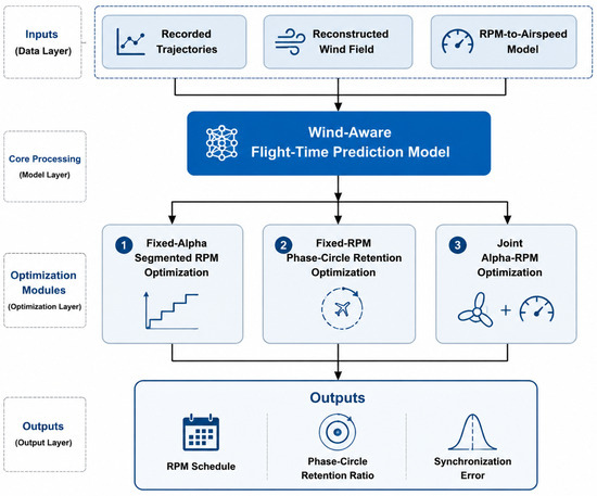
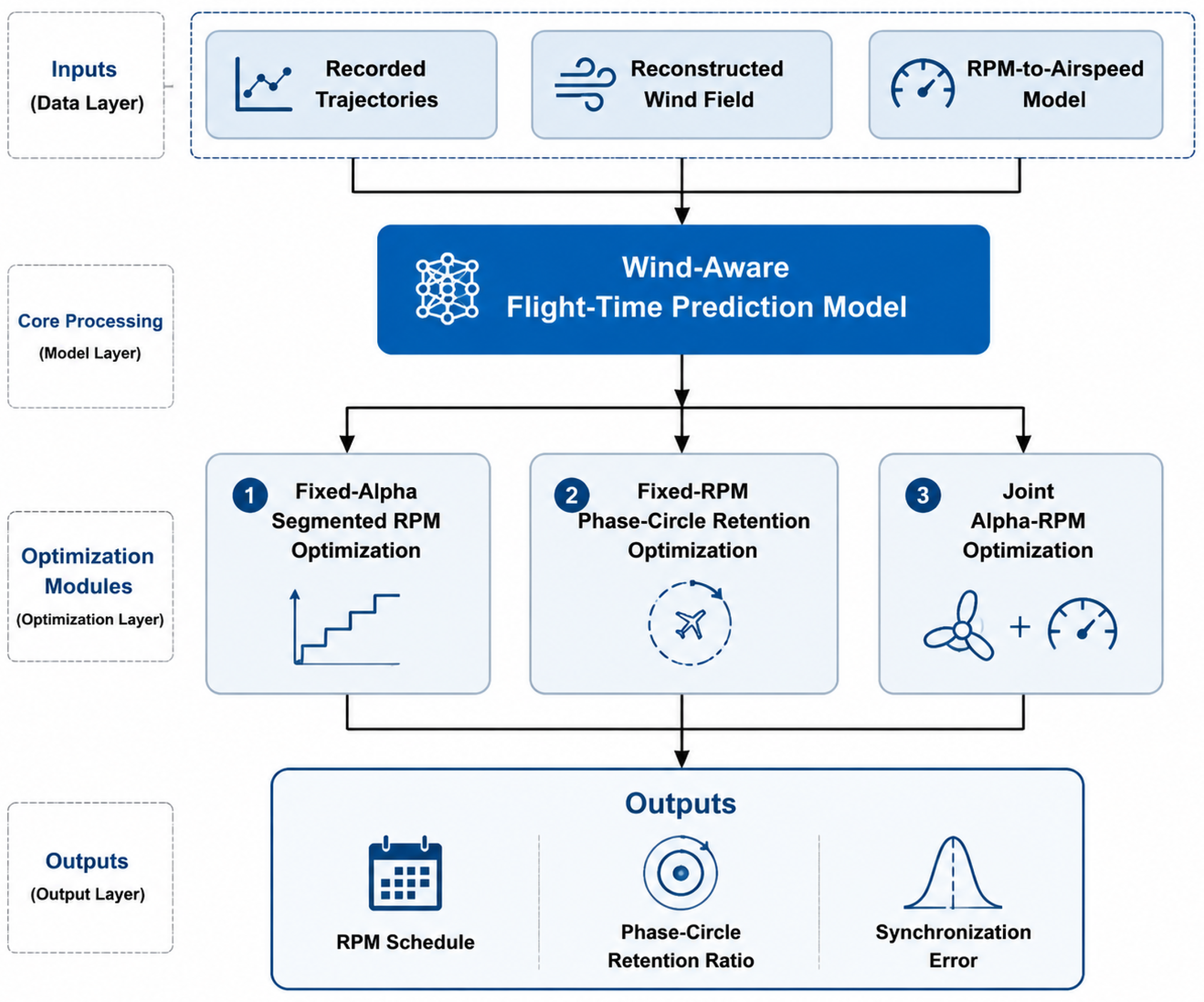
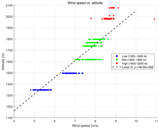
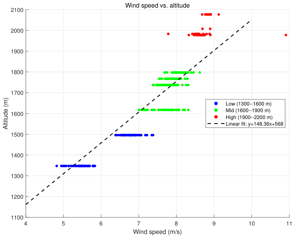
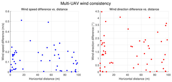
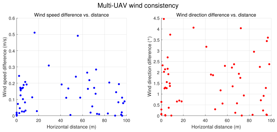
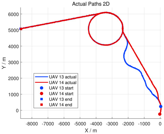
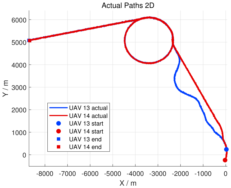
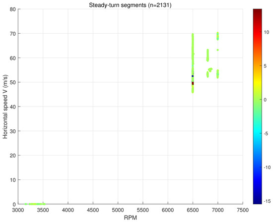
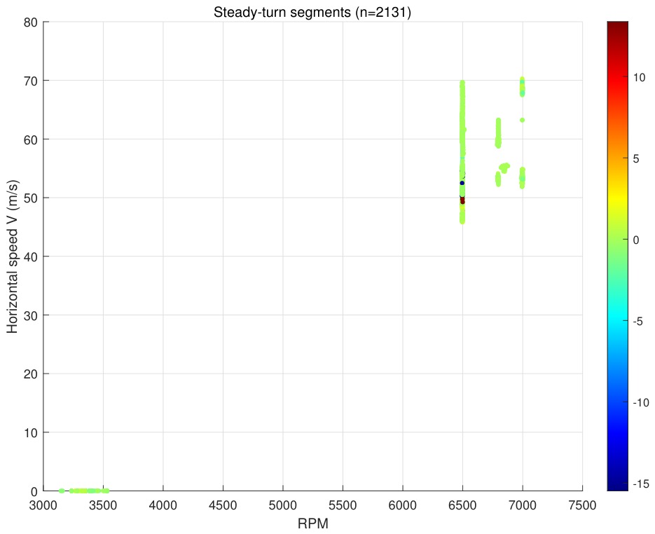
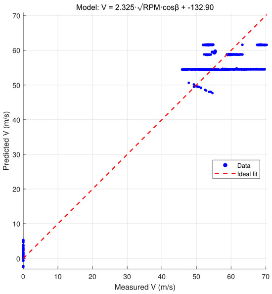
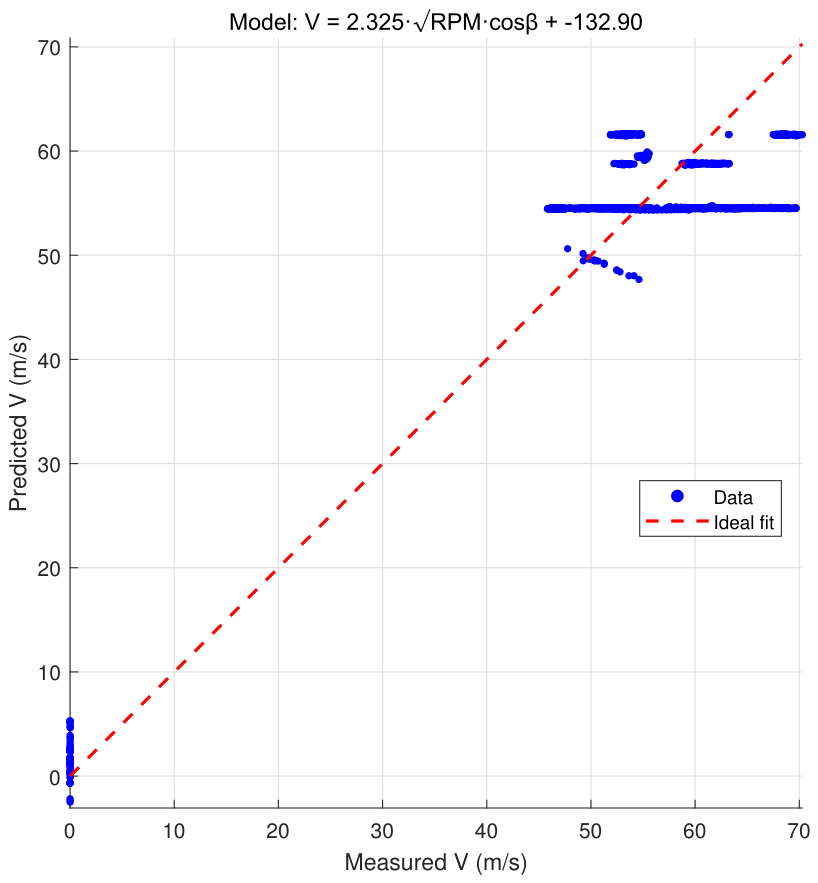
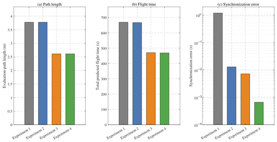
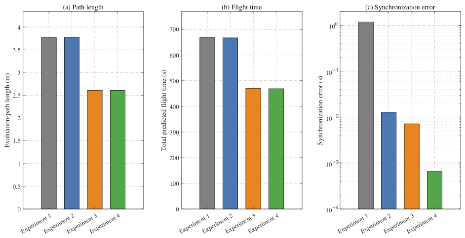
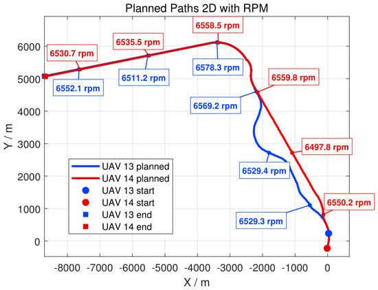
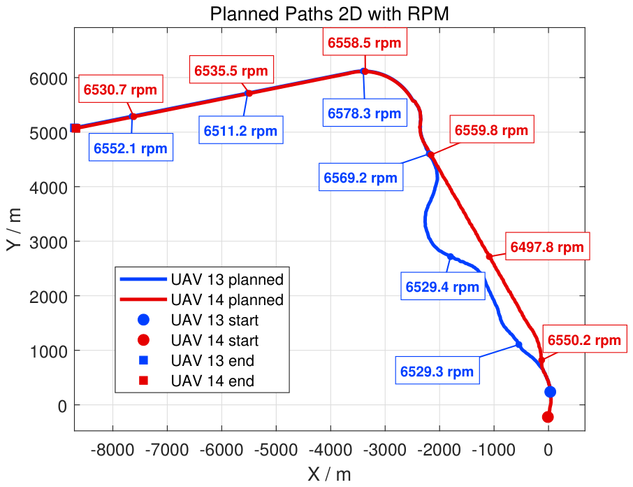

Disclaimer/Publisher’s Note: The statements, opinions and data contained in all publications are solely those of the individual author(s) and contributor(s) and not of MDPI and/or the editor(s). MDPI and/or the editor(s) disclaim responsibility for any injury to people or property resulting from any ideas, methods, instructions or products referred to in the content. |
© 2026 by the authors. Licensee MDPI, Basel, Switzerland. This article is an open access article distributed under the terms and conditions of the Creative Commons Attribution (CC BY) license.