


Highlights
What are the main findings?
- A novel hybrid path planning framework (Improved A* + Enhanced APF) is proposed for seamless UAV navigation across continuous indoor–outdoor environments.
- The proposed algorithm achieves a significant reduction in average turning angles while maintaining optimal path efficiency and successfully escaping local minima traps.
What are the implications of the main findings?
- The significant reduction in sharp maneuvers contributes to maintaining payload stability and cargo safety, addressing a critical physical constraint in UAV logistics.
- This collaborative framework bridges the gap between indoor warehouse and outdoor urban planning, providing a robust and scalable solution for autonomous “last-mile” delivery.
Abstract
Path planning for cargo unmanned aerial vehicles (UAVs) in continuous indoor–outdoor heterogeneous environments poses a critical challenge: promoting payload stability under sharp turns and abrupt altitude variations while maintaining navigational efficiency. To address this issue, this paper proposes a hybrid A*–APF path planning framework that embeds trajectory smoothness optimization directly into the planning process rather than treating it as a post-processing step. An improved A* algorithm is developed by incorporating a trajectory smoothness term into its cost function to penalize sharp turns during global path generation. The resulting path is further refined using an enhanced artificial potential field (APF) method with virtual target points and multi-field force synthesis to mitigate local minima. In addition, the Ramer–Douglas–Peucker algorithm is employed to remove redundant waypoints, and a trajectory generation module based on B-spline interpolation and minimum snap optimization is introduced to produce smooth and dynamically feasible trajectories. Numerical simulation results demonstrate that, in indoor warehouse environments, the proposed method reduces the average turning angle by 88.4% (to 23.1°) compared with the standard A* algorithm while maintaining a comparable path length of 135.11 m. In large-scale outdoor urban scenarios, it achieves a path smoothness of 0.0124 with an average turning angle of 40.0°, substantially outperforming the Genetic Algorithm (104.6°) and Particle Swarm Optimization (83.5°) on turning angle while delivering competitive computation times of 0.52–1.51 s. An ablation study confirms that the improved A* and enhanced APF components each contribute independently to turning angle reduction and local minima avoidance, respectively, and that their integration yields the optimal balance across all metrics. These results indicate the proposed framework’s effectiveness for UAV-based last-mile delivery in scenarios requiring seamless indoor–outdoor transitions under payload stability constraints.
1. Introduction
With the rapid advancement of unmanned aerial vehicle (UAV) technology and the progressive relaxation of regulatory frameworks governing low-altitude airspace, drone-based logistics has emerged as a transformative solution to address the escalating demand for efficient last-mile delivery—the terminal segment of the supply chain in which goods are transported from a distribution hub or warehouse to the end customer. Last-mile delivery is widely recognized as the most cost-intensive and operationally challenging phase of logistics, accounting for up to 53% of total shipping costs, primarily due to traffic congestion, labor shortages, and the spatial dispersion of urban and suburban delivery points [1]. Compared with conventional ground transportation, UAVs offer distinct advantages in this context: they are inherently immune to road-network constraints, capable of flying direct geodesic routes, and can achieve significantly shorter delivery times over short-to-medium distances. These operational benefits have motivated large-scale deployment initiatives by major logistics operators, including Amazon Prime Air, Google Wing, and DHL Parcelcopter, and have spurred an extensive body of research on UAV path planning for urban and semi-urban delivery scenarios [2].
Despite the considerable progress achieved in UAV path planning, existing studies have predominantly addressed indoor and outdoor environments in isolation, resulting in a fragmented body of knowledge that does not reflect the operational reality of end-to-end logistics. Indoor navigation methods typically emphasize high-precision localization, dense environmental mapping, and robust obstacle avoidance under GPS-denied conditions, as exemplified by SLAM-based frameworks [3,4], UWB-AOA/IMU fusion approaches [5], and grid-optimized planning strategies tailored for structured warehouse environments [6,7]. These methods, however, rely on centimeter-level mapping fidelity and are inherently constrained to small-scale, enclosed spaces; their dependence on dense grid representations (with resolutions on the order of 1 m or finer) renders them computationally prohibitive and representationally inadequate for outdoor urban-scale deployment [8]. Conversely, outdoor UAV path planning research has focused on large-scale navigation, energy-aware trajectory optimization, and multi-agent coordination under environmental uncertainties. Representative works include hybrid metaheuristic optimization frameworks [9,10], consensus-based swarm coordination algorithms [11], and coverage path planning for aerial fleets [12], as well as safe navigation strategies under GNSS signal degradation in urban canyons [13]. While these approaches exhibit strong performance in kilometer-scale environments, they generally adopt coarse environmental discretizations (e.g., 20 m grid cells) and assume relatively sparse obstacle distributions, lacking the precision required for confined indoor maneuvering. Critically, the heterogeneous nature of the indoor–outdoor boundary—involving abrupt transitions in spatial scale, coordinate reference frames, obstacle density, and navigation sensor modalities—has received minimal systematic treatment in the literature, leaving a significant gap in the development of unified, continuous-domain planning frameworks [8,12].
In addition to the indoor–outdoor fragmentation, a second and equally critical limitation pervades the existing path planning literature: the systematic neglect of task-specific physical constraints, particularly payload stability. The overwhelming majority of conventional planning algorithms—whether graph-based, sampling-based, or optimization-based—optimize geometric criteria such as path length, obstacle clearance, or computational efficiency, treating the UAV as a point-mass agent whose orientation and dynamic state are irrelevant to planning performance [14,15]. For cargo UAVs engaged in suspended-payload or top-mounted delivery operations, this simplification is fundamentally inadequate. Payload dynamics are highly sensitive to aggressive maneuvers: sharp turns induce lateral centrifugal forces that can excite pendulum-like swinging of suspended loads, while abrupt altitude changes generate vertical accelerations that may compromise cargo integrity or trigger load detachment [16]. The consequences of neglecting such constraints extend beyond theoretical suboptimality—they directly threaten mission safety, delivery reliability, and public acceptance of urban UAV logistics. Despite the well-documented sensitivity of slung-load systems to maneuver aggressiveness in the aerospace and rotorcraft literature [17], the explicit incorporation of payload stability metrics into the core path planning objective—rather than as a posteriori verification—remains largely unaddressed in the UAV navigation domain.
It is important to distinguish the approach proposed in this work from the widespread practice of trajectory smoothing as a post-processing step applied after path generation. In many existing frameworks, a collision-free path is first computed using a conventional planner (e.g., A*, RRT*, or a metaheuristic search), after which spline interpolation, minimum-snap optimization, or Bézier curve fitting is applied to smooth the resulting waypoint sequence and improve dynamic feasibility [18,19]. While computationally convenient, this decoupled paradigm suffers from a structural limitation: the initial path search is conducted without any awareness of smoothness as a planning objective, and consequently the optimizer may irrevocably commit to a geometrically short path whose topology—such as a sequence of zigzag segments through densely packed obstacles—is inherently tortuous and cannot be adequately smoothed without either violating obstacle clearance constraints or substantially deviating from the original route. In other words, post-processing can soften the corners of a path, but it cannot fundamentally alter the path’s structural character. For cargo UAV operations, this distinction is of practical significance: a path that appears acceptable after post hoc smoothing may still contain residual heading changes of sufficient magnitude to excite payload oscillations, because the planner never evaluated kinematic smoothness during the search itself. In contrast, directly embedding a trajectory smoothness term into the cost function of the search algorithm—as is done in the improved A* component of the proposed framework—ensures that the exploration process inherently favors path topologies that are structurally amenable to smooth execution, eliminating the discrepancy between planned geometry and dynamic feasibility at the source.
Taken together, the foregoing analysis identifies three interrelated gaps in the current state of the art. First, a unified planning framework capable of supporting seamless transitions between indoor and outdoor environments—reconciling disparate spatial resolutions, environmental representations, and constraint regimes within a single algorithmic pipeline—has yet to be established [8,12]. Second, path smoothness and payload stability are predominantly treated as secondary concerns, addressed after path generation through post-processing heuristics, rather than being embedded as first-class objectives within the planning stage itself [18,19]. Third, the integration of global path search, local collision avoidance, and kinodynamically aware trajectory generation into a coherent, end-to-end framework remains an open challenge, particularly for large-scale, heterogeneous operational domains that impose both geometric and physical constraints on feasible flight trajectories [15,20]. These gaps collectively motivate the present study.
To address the identified limitations, this study develops a hybrid and stability-aware path planning framework for UAV operations in continuous indoor–outdoor environments. The framework comprises three tightly integrated algorithmic modules. First, an improved A* algorithm is developed that incorporates a trajectory smoothness penalty term directly into its cost function, ensuring that the global path search inherently biases exploration toward smooth, low-curvature route topologies rather than merely optimizing for path length. Second, the resulting global path is locally refined using an enhanced artificial potential field (APF) method augmented with virtual target points and multi-force field synthesis to resolve local minima entrapment—a well-known failure mode of classical APF formulations—while preserving the smoothness properties inherited from the improved A* stage. Third, the Ramer-Douglas-Peucker (RDP) algorithm is employed to eliminate redundant waypoints, and a trajectory generation module based on B-spline interpolation and minimum-snap optimization produces a continuous-time trajectory that satisfies dynamic feasibility constraints. A dedicated boundary transition mechanism—incorporating a structurally defined exit zone, a constraint-aware vertical ascent segment, and resolution-matched trajectory concatenation—enables seamless navigation across the indoor–outdoor interface without manual intervention or environmental re-initialization.
Compared with the state-of-the-art, the primary contributions of this work are as follows:
- A Unified Indoor–Outdoor Planning Framework: A seamless path planning architecture is proposed and implemented that integrates fine-resolution indoor grid maps with coarse-resolution outdoor 3D models, connected through a structured boundary transition mechanism. In contrast to prior studies that address indoor and outdoor navigation as independent problems [6,12], the proposed framework generates a single, globally continuous trajectory across heterogeneous domains without requiring domain-specific reconfiguration.
- Stability-Aware Path Optimization via Embedded Smoothness: To address the critical but underexplored issue of payload stability in UAV logistics, a trajectory smoothness metric is embedded directly into the cost function of the A* search algorithm, explicitly penalizing sharp turns and abrupt altitude changes during path exploration. This design fundamentally differs from post-processing-based smoothing approaches [18,19], as it constrains the search to path topologies that are structurally compatible with smooth execution, thereby promoting payload safety throughout the delivery mission.
- Hybrid Algorithm Design with Complementary Strengths: An innovative integration of an improved A* algorithm and an enhanced APF method is introduced, combining the global optimality and determinism of heuristic graph search with the local responsiveness of potential-field-based obstacle avoidance. The APF component is augmented with virtual target points and multi-force synthesis to overcome the classical local minima problem, achieving a pragmatic balance between global path efficiency and real-time local adaptability.
- Comprehensive Numerical Benchmarking and Performance Characterization: Extensive simulation-based evaluation is conducted across both structured indoor warehouse environments and large-scale outdoor urban scenarios in MATLAB R2024a. The proposed method is systematically benchmarked against representative graph-based, sampling-based, and metaheuristic path planning algorithms, with performance characterized along multiple dimensions including path smoothness (quantified via average turning angle reduction), path length, computational runtime, and local minima escape capability. While the current validation is limited to numerical simulation, the evaluation scenarios are designed to capture realistic operational constraints, and the results provide a rigorous baseline against which future software-in-the-loop (SITL) and hardware-in-the-loop (HIL) validations on established flight stacks (e.g., PX4 and ArduPilot) can be measured.
The remainder of this paper is organized as follows. Section 2 critically reviews the related literature and positions the present work relative to prior contributions. Section 3 formalizes the problem statement and constraint model. Section 4 describes the proposed hybrid planning framework in detail. Section 5 presents the simulation setup, comparative results, and performance analysis. Section 6 discusses the implications, limitations, and future research directions, and Section 7 concludes the paper.
2. Related Work
This section critically examines the existing literature across four thematic areas relevant to the proposed framework: global path planning paradigms, indoor–outdoor cross-domain navigation, trajectory smoothing and stability-aware planning, and the positioning of the present work relative to prior contributions. Unlike a conventional survey, the analysis below emphasizes the limitations of each category of methods, establishing the specific research gaps that motivate and justify the hybrid framework developed in this study.
2.1. Global Path Planning
UAV path planning has been extensively investigated through four dominant algorithmic paradigms: graph-based search, sampling-based exploration, bio-inspired and metaheuristic optimization, and learning-based methods. Rather than rehearsing the well-documented mechanics of each paradigm, this section focuses on their structural limitations when applied to cargo UAV operations in heterogeneous environments.
Graph-based methods, exemplified by A* and its derivatives (e.g., D*, Theta*, and Jump Point Search), operate on discretized grid representations and offer deterministic optimality guarantees with respect to the defined cost metric [4]. Their principal advantage—completeness and repeatability—is, however, obtained at the expense of angular resolution: because the search is confined to grid-adjacent transitions (typically multiples of 45° in 2D grids), the resulting paths are inherently piecewise linear with abrupt heading changes at waypoints. For cargo UAVs, such discontinuous curvature profiles directly translate into aggressive yaw maneuvers that excite payload oscillations. Post-grid smoothing can partially mitigate this effect, but the fundamental limitation resides in the decoupling of geometric search from kinematic feasibility assessment.
Sampling-based methods, most notably RRT, RRT*, and their informed variants, avoid explicit grid discretization by constructing connectivity graphs through stochastic exploration of the configuration space [5]. This property renders them effective in high-dimensional and cluttered environments where grid-based methods suffer from the curse of dimensionality. However, the stochastic nature of sampling introduces two related deficiencies for logistics applications. First, path quality is non-deterministic: repeated runs of the same planner on the same environment may yield topologically distinct paths with substantially different smoothness profiles, undermining the predictability required for certified delivery operations. Second, the raw paths produced by sampling-based planners are almost invariably jagged and require dedicated post-processing to achieve curvature continuity, reintroducing the decoupling problem.
Bio-inspired and metaheuristic optimization algorithms, including PSO, GA, grey wolf optimization (GWO) [7], fruit fly optimization [6], and sparrow search algorithms [8], formulate path planning as a multi-objective optimization problem over a continuous parameter space. These methods can naturally accommodate diverse cost terms within a single objective function, and their population-based search strategy reduces susceptibility to local minima. Nevertheless, their computational footprint is substantial, rendering them unsuitable for real-time replanning in dynamic delivery environments. Furthermore, the stochastic nature of their convergence makes it difficult to provide formal guarantees on path optimality or constraint satisfaction.
Learning-based methods, including deep reinforcement learning (DRL) [10] and deep learning-based obstacle avoidance [9], have demonstrated remarkable adaptability to unseen environments. However, their reliance on extensive training datasets and their fundamental opacity with respect to safety guarantees severely limit their applicability to cargo UAV operations, where an errant policy update can result in payload loss. The well-documented fragility of DRL policies to distributional shift further compounds these concerns in heterogeneous indoor–outdoor settings [10].
Regardless of the paradigm, a common deficiency pervades the aforementioned methods: none of them embed payload stability or trajectory smoothness as a first-class objective within the path search process. Geometric optimality (shortest path) and computational efficiency remain the dominant optimization criteria, while the kinematic consequences of the planned path on the transported cargo are either ignored entirely or deferred to a decoupled post-processing stage. This observation motivates the first design principle of the proposed framework: the integration of a smoothness penalty directly into the heuristic cost function of the global planner.
2.2. Indoor–Outdoor Cross-Domain Navigation
The operational reality of UAV-based logistics demands navigation capabilities that span both indoor environments and outdoor environments. Existing research, however, has almost exclusively treated these two domains as separate problems, resulting in a bifurcated literature that offers no systematic solution for the indoor–outdoor transition.
Indoor UAV navigation research has focused primarily on localization under GPS-denied conditions and high-precision obstacle avoidance in confined, structured spaces [11,12,13,14]. On the planning side, grid-optimized search strategies [4], BIM-assisted coverage planning [15], and point-cloud-based real-time obstacle avoidance [16] have demonstrated effectiveness in warehouses [17] and agricultural facilities [18]. The unifying characteristic of these methods is their reliance on high-resolution, dense environmental representations, which are computationally intractable and representationally inappropriate for kilometer-scale outdoor domains. Critically, none of the surveyed indoor methods incorporate a mechanism for handing off navigation authority to an outdoor planner at the environment boundary.
Outdoor UAV path planning, conversely, operates at a fundamentally different spatial and representational scale. Research in this domain has emphasized energy-aware trajectory optimization [20], multi-objective planning [21], multi-agent cooperative planning and swarm coordination [22,23,24], and safety-preserving navigation under GNSS signal degradation [25]. Emerging approaches have also explored the integration of large language models for visual path reasoning [26] and noise-exposure-constrained planning [27]. These methods typically assume coarse environmental discretizations (10–20 m grid cells) and continuous GNSS availability. Moreover, their planning architectures are not designed to accept a high-resolution indoor terminal segment as an initial condition.
The boundary involves simultaneous discontinuities in (i) spatial resolution, (ii) environmental representation, (iii) available sensor modalities, and (iv) operational constraints. To the best of our knowledge, no existing framework provides a unified planning pipeline that reconciles all four dimensions of heterogeneity within a single, computationally tractable architecture. The transition mechanism designed in this work is specifically engineered to bridge this gap.
2.3. Trajectory Smoothing and Stability-Aware Planning
Trajectory smoothness has been recognized as an important consideration in UAV path planning. However, the manner in which smoothness is incorporated into the planning pipeline varies considerably across the literature.
Post-processing approaches constitute the predominant paradigm. A geometric path is first generated by a conventional planner, after which a smoothing algorithm (e.g., B-spline and minimum-snap) is applied to the waypoint sequence [18,19,21]. This decoupled architecture offers practical convenience but introduces an irreducible structural limitation: the path planner may commit to a route topology that is inherently tortuous, and the smoother cannot fundamentally restructure the path without violating obstacle clearance. The result is a trajectory that may retain residual heading changes of sufficient magnitude to excite payload dynamics.
Simultaneous planning and smoothing approaches incorporate smoothness metrics directly into the planning objective [28,29]. While these represent a conceptual improvement, their application has been largely confined to single-domain scenarios. Furthermore, the smoothness criteria employed (typically curvature or jerk minimization) are generic kinematic metrics that do not explicitly model the coupling between path geometry and payload dynamics specific to cargo UAVs.
Payload stability in UAV path planning has received surprisingly limited attention. Studies typically address payload behavior at the control level (e.g., active pendulum damping controllers) rather than at the planning level. Collaborative truck-drone routing frameworks [30] and energy-consumption-aware planning models [20] abstract away the kinematic details of individual UAV trajectories. Consequently, generating paths inherently compatible with payload stability remains an open research problem.
Table 1 provides a structured comparison of representative trajectory planning and smoothing methods.
Table 1.
Comparative analysis of representative trajectory planning and smoothing methods.
As Table 1 illustrates, no existing method simultaneously satisfies all four criteria. The proposed framework is designed to occupy this unfilled cell in the design space.
2.4. Positioning of the Present Work
The critical analysis presented in Section 2.1, Section 2.2 and Section 2.3 identifies a coherent set of research gaps that the proposed framework is specifically designed to address:
- From decoupled to embedded smoothness: Whereas the dominant paradigm treats trajectory smoothness as a post-processing correction, the proposed framework embeds a smoothness penalty (the term) directly into the heuristic cost function of the improved A* algorithm.
- From domain-specific to cross-domain unified planning: Whereas existing methods are designed for either indoor or outdoor environments in isolation, the proposed framework introduces a structured boundary transition mechanism.
- From geometry-only to stability-aware optimization: Whereas conventional planners optimize purely geometric criteria, the proposed framework explicitly incorporates payload stability constraints (turning angle, flight-path inclination, and flight range) into the planning objective.
- From isolated to integrated local-global refinement: Whereas most frameworks deploy global planning and local obstacle avoidance as loosely coupled modules, the proposed framework tightly integrates the improved A* global planner with an enhanced APF local refinement stage.
In summary, the present work contributes a co-design of the global search objective, the local refinement mechanism, the cross-domain transition architecture, and the trajectory generation pipeline, unified by the overarching design principle that payload stability must be a first-class consideration at every stage of the planning process.
3. Problem Modeling and Constraint Analysis
3.1. Environmental Modeling
Let a path be represented by a sequence of waypoints (), where () is the start point and () is the goal point. Each waypoint () specifies the three-dimensional position. The path planning problem is formulated as minimizing the total path length [31]:
subject to the operational constraints defined in Section 3.2. The index starts from 0 so that the segment-wise operations in turning-angle computation (Equation (3)), RDP simplification, and B-spline trajectory generation (Section 4.3) consistently operate on adjacent segment pairs ().
The problem defined by Equation (1) belongs to the class of constrained shortest-path problems on a three-dimensional occupancy grid. Let the workspace be discretized into a uniform grid with resolution $r$. Each cell is labeled as either traversable () or occupied (), collectively forming an occupancy map . A path is feasible if and only if (i) every waypoint lies in a traversable cell, (ii) the straight-line segment between consecutive waypoints intersects no occupied cell, and (iii) the sequence satisfies the kinematic, energy, and operational constraints formalized in Section 3.2.
The problem is distinguished from conventional shortest-path formulations by the heterogeneous nature of the workspace: the environment may comprise multiple sub-domains that differ in spatial scale, grid resolution, obstacle morphology, and prevailing navigation constraints. Each sub-domain is characterized by an occupancy map at resolution . The sub-domains are coupled through a set of boundary regions that define spatial adjacency and constrain feasible transitions between adjacent domains. The path must remain feasible within each sub-domain individually and across all inter-domain boundaries. This multi-domain structure is motivated by the “last-mile” delivery scenario, wherein a UAV must navigate seamlessly from a confined indoor warehouse () through a transition zone () into a large-scale outdoor urban airspace (), and vice versa [32].
To evaluate the proposed framework under diverse operational conditions, two representative environments are modeled: an indoor warehouse and an outdoor urban setting. The modeling parameters for these environments are summarized in Table 2.
Table 2.
Key Modeling Parameters of Indoor Warehouse and Outdoor Urban Environments.
The indoor warehouse environment was represented using a three-dimensional grid map, with the Z-axis fixed at 1 m, and the core region modeled as a two-dimensional traversable area. The overall dimensions of the warehouse were set to 100 m × 100 m × 5 m, with a minimum clearance height of 4.5 m to ensure safe UAV passage. The grid resolution was set at 1 m per cell, balancing path planning precision and computational efficiency, and effectively avoiding unnecessary computational overhead caused by excessive grid refinement.
Obstacles were arranged uniformly along the X-axis at 20, 40, 60, and 80 m and along the Y-axis at 10, 30, 50, 70, and 90 m, with adjacent shelves spaced 8 m apart. The warehouse contained a total of 20 obstacle groups, including shelves and walls, represented as ‘1’ for obstacles and ‘0’ for traversable areas. The start point was positioned near the warehouse entrance at coordinates [5, 5, 1], ensuring sufficient clearance from obstacles and adequate takeoff space. The goal point was set near the warehouse exit at coordinates [95, 95, 1], connected to the outdoor transition point. The indoor warehouse environment model is illustrated in Figure 1.
Figure 1.
Indoor Warehouse Environment Model.
The outdoor urban environment was modeled using a three-dimensional grid map, with buildings represented as precise cuboid obstacles. This environment encompassed the scale of a typical city block, with dimensions of 2000 m × 2000 m × 100 m, providing adequate low-altitude flight space. To accommodate the large-scale urban setting, the grid resolution was set to 20 m per cell, preventing excessive memory consumption caused by over-refined grids.
Obstacles included approximately 100 buildings, randomly distributed throughout the area while ensuring no overlap with delivery or transition points. The minimum spacing between buildings was maintained at 15 m to satisfy lateral obstacle avoidance safety requirements. Unlike the indoor environment, the outdoor scenario did not have a distinct start point; instead, a transition point served as the starting location for outdoor path planning, positioned at [100, 100, 5], a critical juncture connecting indoor and outdoor paths.
Within the outdoor environment, five delivery points were designated at the following coordinates: (43.5, 849.5, 30.0), (538.5, 1504.5, 42.0), (1715, 1780, 50.0), (1660, 465, 65.0), and (1115, 1053, 90.0). Additionally, an auxiliary takeoff node was pre-set at [100, 100, 25], located 10 m vertically above the transition point, serving as the formal starting point for outdoor path execution. The modeled urban environment is illustrated in Figure 2.
Figure 2.
Outdoor Urban Environment Model.
The indoor and outdoor environments are spatially coupled through a shared boundary region. The indoor goal point () is located at the warehouse exit, while the outdoor transition point () and an auxiliary takeoff point () (positioned 10 m vertically above the transition point) serve as the entry to the outdoor path. The proximity of these boundary coordinates (approximately 5 m horizontally between the indoor goal and the outdoor transition point) ensures that the two path segments can be joined without an extensive intermediate traversal.
3.2. UAV Model and Constraints
This study considers a multi-rotor (quadcopter) UAV platform. Unlike fixed-wing UAVs, multi-rotors can hover and perform vertical maneuvers; however, payload stability remains sensitive to aggressive translational maneuvers. The key mathematical symbols and their definitions used in this study are listed in Table 3.
Table 3.
The Key Mathematical Symbols and Their Definitions.
In this study, a quadrotor UAV is employed as the transport platform, with its physical parameters and performance constraints summarized in Table 4. When carrying a payload, the UAV’s dynamic characteristics change, necessitating consideration of the following key constraints:
Table 4.
UAV System Parameters and Constraints.
3.2.1. Lateral Acceleration Constraint
For cargo UAVs, the fundamental physical constraint governing turning maneuvers is lateral acceleration rather than the turning angle per se, as it is the centrifugal force—proportional to lateral acceleration—that induces payload swing and threatens load stability [33]. Denoting the instantaneous flight speed by (v) and the heading angular rate by (), the lateral acceleration is defined as:
To prevent excessive lateral perturbation of the payload, is bounded by a safe upper limit :
For the multi-rotor platform considered here (, Table 4), a conservative limit of is adopted. Following previous studies on cargo UAV operation [17,33], a lateral acceleration limit in the range of 0.2–0.3 g is commonly adopted to suppress payload oscillation and maintain cargo integrity during translational maneuvers; the value of 0.25 g selected here lies within this established range and is commensurate with typical cargo stability margins for small multi-rotor UAVs. The corresponding angular rate bound is:
which is conservatively rounded to 30°/s as the operational threshold enforced in the planning algorithm.
It should be noted that the derivation above adopts a constant cruise-speed assumption for planning purposes. In general, the lateral acceleration bound yields a speed-dependent angular rate limit:
where v denotes the instantaneous cruise speed. Under this generalized formulation, a lower flight speed permits a proportionally higher heading rate, whereas a higher speed necessitates gentler turns to maintain the same lateral acceleration threshold. The present study adopts as a nominal cruise speed to maintain consistency across all simulation scenarios. This constant-speed simplification decouples the trajectory geometry search from speed profile optimization, thereby reducing the dimensionality of the planning problem while maintaining a consistent lateral-acceleration limit throughout the planned trajectory. Extension of the framework toward adaptive-speed planning—wherein the cruise velocity is jointly optimized with the path geometry—constitutes a natural direction for future work.
In grid-based path planning, the lateral acceleration constraint must be expressed in a computationally tractable geometric form. For any three consecutive waypoints , the segment vectors are:
The inter-segment turning angle is:
and is constrained by:
This equation is the geometric analogue of the lateral acceleration bound: given a fixed control interval , the per-step heading change inherits the same limit.
To guide the global search toward paths that inherently satisfy the lateral acceleration constraint, a turning smoothness penalty is embedded in the A* cost function:
where is a weighting coefficient (set to 0.5). The penalty structure is designed to vanish for straight-line flight, apply moderate cost to gradual turns, and maximally penalize sharp heading changes, thereby steering the search away from path segments likely to violate the lateral acceleration bound.
3.2.2. Flight Range Constraint
The maximum flight range of a UAV is dictated by its onboard energy capacity (battery or fuel). If the cumulative trajectory length exceeds this limit, the UAV will deplete its energy reserve before completing the mission, resulting in mission failure. The constraint is therefore formulated as an energy-feasibility condition:
where (Table 4). Satisfaction of this equation indicates that the planned path is expected to be executable within the platform’s energy budget.
Under the constant cruise-speed assumption introduced in Section 3.2.1, the flight range constraint is mathematically equivalent to a flight time constraint, since . Nevertheless, the distance-based formulation is retained in the present work for two reasons. First, the path planning algorithm directly optimizes the cumulative Euclidean path length as its primary objective (Equation (1)); expressing the endurance limitation in terms of travel distance therefore maintains dimensional consistency between the optimization objective and the feasibility constraint. Second, the geometric path length is an intrinsic property of the planned trajectory, independent of the speed profile adopted during execution; the corresponding flight time can be recovered a posteriori once the speed schedule is determined. This decoupling allows the range constraint to remain applicable even if the speed assumption is relaxed in future extensions.
3.2.3. Flight-Path Inclination Constraint
During three-dimensional trajectory planning, excessively steep climb or descent segments may lead to abrupt altitude transitions between consecutive waypoints, thereby reducing the smoothness and practical feasibility of the planned trajectory. To generate smoother three-dimensional paths while considering payload transportation requirements, a flight-path inclination constraint is introduced.
Unlike the vehicle pitch angle, which is defined with respect to the UAV body frame and depends on the flight controller and attitude dynamics, the flight-path inclination angle considered in this study is a purely geometric quantity determined by the spatial relationship between consecutive waypoints. Therefore, it is introduced as a planning-level geometric constraint rather than an explicit vehicle-attitude or payload-dynamics constraint.
where , and denote the coordinate differences between two adjacent waypoints.
To avoid excessively steep altitude transitions, the inclination angle is constrained by
The threshold provides a conservative margin that limits the horizontal component of payload displacement during altitude changes, thereby preserving load stability without excessively restricting the platform’s vertical maneuverability.
It should be emphasized that the proposed flight-path inclination constraint is formulated at the trajectory-planning level rather than the flight-dynamics level. The inclination angle defined in Equation (12) represents the geometric relationship between consecutive waypoints and should not be interpreted as the UAV body pitch angle, which depends on the vehicle body frame, attitude controller, and aerodynamic characteristics. Accordingly, the proposed constraint serves as a planning-level geometric constraint to regulate altitude transitions during trajectory generation. Although smoother trajectories may contribute to improved payload transportation stability, the proposed formulation does not explicitly model vehicle attitude or payload dynamics.
3.2.4. Flight Altitude Constraint
The flight altitude constraint imposes a critical limitation on the UAV’s operational altitude, ensuring that the vehicle remains within a predefined safe altitude range. This not only facilitates compliance with regulatory and obstacle avoidance requirements but also mitigates the occurrence of frequent altitude fluctuations. As a result, the continuity and smoothness of the UAV’s trajectory are preserved, enhancing mission performance and operational safety.
Formally, the altitude constraint is defined as:
where Hi denotes the UAV’s altitude at the i-th waypoint, and and specify the UAV’s minimum and maximum permissible flight altitudes, respectively.
The four constraints defined above are enforced at different stages of the planning pipeline:
- Hard feasibility filters: The flight-path inclination constraint and flight altitude constraint () are enforced as hard feasibility checks during node expansion in both the global A* search and the local APF refinement: any candidate waypoint violating either constraint is pruned immediately. This ensures that every waypoint in the generated path is altitude- and inclination-angle-feasible by construction.
- Soft penalty: The lateral acceleration constraint is enforced as a soft penalty via embedded in the A* cost function. Unlike hard constraints, which would render large portions of the search space infeasible in cluttered environments, the soft penalty formulation allows the planner to accept minor violations when geometrically unavoidable while strongly favoring paths with inherently low lateral acceleration.
- Global feasibility check: The flight range constraint is verified after the complete path is generated. If , the path is rejected and re-planning is triggered with a reduced search radius. Given the platform’s 15 km range budget and the environment scales considered, this condition is rarely active but serves as a safety backstop.
3.3. Objective Evaluation Function
The performance of a UAV path-planning algorithm is evaluated along three dimensions: path efficiency, computational tractability, and trajectory quality. To capture these dimensions quantitatively, six metrics are defined:
- Path length (m): the cumulative Euclidean distance along the planned trajectory, measuring navigational efficiency.
- Number of nodes : the count of waypoints in the discrete path before smoothing, reflecting path complexity.
- Planning time (s): the wall-clock computation time from algorithm invocation to path output, measuring real-time responsiveness.
- Path smoothness : a dimensionless index quantifying the absence of sharp directional changes, defined below.
- Number of turns : the count of waypoints at which the inter-segment turning angle exceeds a threshold of , measuring maneuver frequency.
- Average turning angle (°): the arithmetic mean of all inter-segment turning angles along the path, measuring maneuver intensity.
Let a path consist of waypoints . For each interior waypoint (), the inter-segment turning angle is defined by Equation (3). The path smoothness is then defined as:
The kernel is adopted to maintain structural consistency with the planning-stage turning penalty defined in Equation (9): . Consequently, minimizing during planning is mathematically equivalent to maximizing in the resulting trajectory—the two quantities share the same angular kernel and differ only in normalization. The metric satisfies , with corresponding to a perfectly straight trajectory and lower values indicating paths containing more frequent or sharper turns. Unlike , which operates within the A* search loop to guide node expansion, is computed post hoc over the final smoothed trajectory and serves purely as an evaluation criterion.
The six raw metrics differ fundamentally in dimension, range, and optimization direction. To aggregate them into a single composite score, a unified two-stage normalization pipeline is applied:
Stage 1 (Direction alignment): For the five metrics that are naturally smaller-is-better (), the direction-aligned quantity is the raw value itself:
For path smoothness, where a larger raw value indicates superior performance, the direction is reversed by taking its complement:
Stage 2 (Min–Max scaling): Every direction-aligned quantity $X’_i$ is then mapped to the unit interval ([0, 1]) via Min–Max normalization:
where and denote the minimum and maximum values of metric observed across all compared algorithms in a given simulation scenario. After Equation (18), every satisfies the smaller-is-better convention, with the best-performing algorithm receiving and the worst receiving .
Applying Stage 2 to rather than to the raw is essential: because by definition (Equation (15)), a Min–Max normalization applied directly to would destroy its intrinsic bounding and create an artificial distributional mismatch with the other five metrics. The two-stage design—direction alignment followed by uniform scaling—preserves the structural integrity of every metric while ensuring dimensional homogeneity in .
Composite objective function. The six normalized metrics are aggregated into a single scalar score:
subject to .
The weight vector is designed to reflect the operational priorities of cargo UAV delivery:
- : Path length is the primary determinant of energy consumption and mission duration.
- : Smoothness directly governs payload stability and is assigned the second-highest weight.
- : Node count reflects path complexity and discretization overhead.
- : Average turning angle captures the aggregate maneuver intensity experienced by the payload.
- : Planning time affects responsiveness to dynamic replanning requests; its lower weight reflects the offline nature of global planning in logistics operations.
- : Turn count is partially redundant with $A$ and $S$ and is accordingly assigned the lowest weight.
Substituting the weights into Equation (18) yields the operational form:
where a smaller value of indicates superior overall performance.
The sensitivity of algorithm ranking to moderate perturbations of this weight vector was examined. Across weight variations of $\pm 0.05$ for each coefficient (with renormalization), the proposed Hybrid A*–APF framework retained the lowest composite score $F$ in all tested configurations. A systematic sensitivity analysis of the trajectory smoothness weight within the A* cost function is presented in Section 5.3.
4. Path Planning Methodology
Building on the problem formulation and constraints defined in Section 3, the proposed path planning framework comprises three tightly coupled modules:
- (1)
- A global path planning module based on an improved A* algorithm with a stability-aware cost function (Section 4.1),
- (2)
- A local path refinement module using an enhanced APF method with multi-field force synthesis and local-minima escape mechanisms (Section 4.2),
- (3)
- A trajectory generation module that produces smooth, dynamically feasible paths via B-spline interpolation and minimum-snap optimization (Section 4.3).
The overall architecture and data flow among these modules are illustrated in Figure 3.
Figure 3.
Hybrid A*–APF Path Planning Framework.
4.1. Improved A* Algorithm
To adapt the A* algorithm for UAV cargo missions, three key improvements are introduced, focusing on path quality, environmental awareness, and search efficiency.
4.1.1. Improvement of the Cost Function
Traditional A* minimizes path length, ignoring trajectory smoothness. For cargo UAVs, abrupt turns can compromise payload stability. This engineering constraint is explicitly addressed by integrating a trajectory smoothness optimization term into the A* cost function:
Here, and retain their conventional definitions as the accumulated actual cost and heuristic cost, respectively. The parameter adjusts the weighting of the smoothness term, which is determined to be 1.0 through a detailed sensitivity analysis (see Section 5.3)., and quantifies the turning penalty associated with the current node.
The turning cost is computed based on the angular deviation between consecutive path segments:
where and represent the directional angles of the adjacent path segments, and k serves as a scaling factor modulating the influence of the smoothness term.
Figure 4 illustrates the effectiveness of the proposed path smoothing methodology integrated into the A* algorithm. The 3D (top-left) and 2D (top-right) trajectory plots provide a visual comparison between the original path and the improved path, demonstrating the mitigation of severe turning angles. The bottom-left panel shows the behavior of the turning cost function, which is designed to penalize sharp turns based on a scaling factor. A quantitative validation is presented in the bottom-right panel, where a bar chart comparison of path curvature confirms the enhanced smoothness of the trajectory generated by our proposed method. This improvement causes the algorithm to favor paths with smaller turning angles during the search process, effectively reducing the occurrence of sharp turns, as illustrated in Figure 5. Figure 5 compares the paths before and after the improvement, clearly demonstrating that the modified path exhibits smoother turns. The heuristic component in Equation (21) is further refined in Section 4.1.2 through an adaptive weighting strategy that dynamically adjusts its contribution according to the local obstacle density. In addition, the larger inter-waypoint spacing apparent in the modified path is a direct consequence of the variable step-size strategy introduced in Section 4.1.3: when the remaining distance to the goal is large, a proportionally expanded step accelerates traversal, yielding fewer waypoints than fixed-unit A* search. This sparser distribution does not degrade trajectory quality, because the post-processing pipeline (RDP simplification followed by B-spline interpolation, Section 4.3) reconstructs a continuous trajectory from the discrete waypoint sequence irrespective of nodal density.
Figure 4.
Performance evaluation of the proposed turning-aware A* algorithm for path smoothing.
Figure 5.
Comparison of Paths Using the Improved A* Algorithm (Top: Traditional A*, Bottom: A* with Trajectory Smoothness Optimization).
4.1.2. Adaptive Heuristic Function Strategy
The standard heuristic in Equation (21) is the Euclidean distance from the current node to the goal. In obstacle-dense regions, optimistic distance estimates may mislead the search into infeasible corridors; conversely, in sparse regions, a strong heuristic accelerates convergence. To adapt the heuristic contribution to local environmental complexity, is replaced by an adaptive form that scales the heuristic weight according to the obstacle coverage ratio :
where denotes the obstacle coverage ratio of the bounding rectangle formed by the start and goal coordinates, defined as the ratio of the total obstacle area to the total map area. Substituting this into Equation (21), the complete cost function used in the final implementation is:
The adaptive mechanism operates as follows. When is low (sparse environments), , and the search relies primarily on the heuristic function to accelerate convergence toward the goal. When is high (dense environments), reduces the heuristic weight, causing the algorithm to depend more heavily on the accumulated path cost , thereby mitigating the risk of heuristic estimation errors leading the search into infeasible regions. This adaptive scaling ensures that the balance between exploration and goal-directed expansion is automatically tuned to the local obstacle density without manual parameter adjustment.
Mechanism of Obstacle Coverage Ratio:
As the obstacle coverage ratio increases, the uncertainty and complexity of the environment rise. If a high heuristic weight is maintained in such cases, the algorithm may excessively depend on the estimated direction of the goal, neglecting the impact of obstacles on path feasibility. This could lead the search to get trapped in invalid regions or even converge to a local optimum. By reducing the relative weight of h(n), the search relies more on the accumulated cost g(n), mitigating the influence of heuristic estimation errors and ensuring the feasibility and stability of the generated path.
As shown in Figure 6, in sparse environments (with p = 0.1, p = 0.3), the adaptive heuristic function exhibits a non-monotonic behavior of “first increasing, then decreasing.” This initial “expansion” of the heuristic value helps the algorithm escape local optimal traps caused by U-shaped obstacles. As the environment becomes denser (with p = 0.5, p = 0.8), the adaptive heuristic function tends to provide a more compact and realistic cost estimate. Moreover, as the obstacle coverage ratio P increases, the search efficiency (represented by the blue bars) decreases, as more nodes need to be explored in a more complex environment. However, the path quality (represented by the red curve) significantly improves, indicating that the adaptive strategy intelligently adjusts the search behavior according to the environmental complexity, sacrificing some search speed for higher-quality path solutions in complex environments.
Figure 6.
Adaptive Heuristic Strategy for Improved A* Algorithm Under Varying Obstacle Coverage.
In Figure 7, the heat map in the upper left corner shows the values of the adaptive heuristic function within the 2D space defined by the parameters p and the number of search iterations. The heat map clearly illustrates that areas with high heuristic values (warm colors) are mainly concentrated in regions with low p values and at the beginning of the search, visually confirming that the “expansion” of the heuristic value primarily occurs in sparse environments to overcome local optima. The upper-right graph overlays the evolutionary curves of the heuristic function at different p values, providing a clearer comparison of the decisive impact of p on the function’s shape.
Figure 7.
Mathematical Analysis of Adaptive Heuristic Strategy with Respect to Obstacle Coverage Parameter.
The lower-left graph quantifies the impact of p on the final heuristic values, revealing a clear negative correlation: the simpler the environment (lower p values), the higher the “expansion” of the heuristic value maintained by the algorithm to escape potential traps. The lower-right graph presents the convergence speed analysis, showing that the number of iterations required for the algorithm to converge increases rapidly as p moves from 0 to 0.2, and then stabilizes at a plateau. This indicates that once the environment complexity exceeds a certain threshold, the algorithm’s solving time stabilizes within a predictable range, demonstrating good robustness.
4.1.3. Expansion Node Selection
To enhance search efficiency, a variable step-size strategy is introduced. The expansion step is scaled proportionally to the remaining distance to the goal: when the current node is far from the goal, a larger step accelerates traversal; as the node approaches the goal, the step is progressively reduced to a unit step to preserve accuracy and promote convergence. Taking the -axis as an example (the same principle applies to the - and -axes), the step size is:
where and denote the coordinates of the current node $n$ and the goal node , respectively. The floor operation produces integer grid steps, and the bound to preserve completeness under the grid discretization.
The divisor of 5 in the equation is an empirically tuned hyperparameter that controls the trade-off between search acceleration and path granularity. A smaller divisor produces larger steps and faster search, but risks skipping over narrow passage entrances when the inter-node spacing exceeds the width of traversable corridors. A larger divisor preserves finer granularity at the cost of reduced acceleration. The value 5 was selected through a grid search over {3, 4, 5, 6, 8, 10} on the indoor warehouse scenario (Section 3.1), where shelf aisles are 8 m wide at 1 m grid resolution. Each candidate value was evaluated on three criteria: path length, computation time, and success rate (proportion of runs that found a feasible path to the goal without entrapment). Divisors 3 and 4 reduced computation time but produced occasional failures in cluttered regions by skipping aisle entrances; divisors 6, 8, and 10 yielded marginal improvements in path length (<2%) at the cost of substantially increased search time. The divisor 5 achieved the best balance across all three metrics, providing a meaningful search acceleration while maintaining a success rate of 100% across all test instances.
When , the risk of collision between the UAV and obstacles arises during movement. To address this, the Bresenham line algorithm is employed for collision detection. This approach generates a set of discrete points along the straight line connecting the start and end of a step, and checks whether these points intersect with any obstacles. Consequently, the variable step-size strategy not only improves search efficiency but also ensures path safety. Simulation results confirm that this method is effective in avoiding obstacles while significantly enhancing computational efficiency.
For a candidate expansion with step size , the Bresenham line algorithm is applied to check the line-of-sight occupancy between the current node and the candidate endpoint. If any sampled grid point intersects an obstacle, the expansion is considered unsafe. In this case, we apply a step rollback strategy to maintain completeness: the step size is reduced and re-tested until either a collision-free segment is found or the step size reaches the minimum unit step. If collision persists at the unit step in the same direction, this direction is rejected and the algorithm falls back to standard neighbor expansion. The variable-step expansion procedure is summarized in Algorithm 1.
| Algorithm 1: Variable-step expansion with Bresenham rollback |
|
4.1.4. Search Pruning with Jump Point Search (JPS)
To further mitigate redundancy in grid-based search, Jump Point Search (JPS) is integrated into the global path generation phase. Instead of traversing all 26 neighbors of a node in a 3D grid, JPS systematically prunes redundant expansion points by identifying “jump points” and “forced neighbors”. A jump point is recursively defined based on its neighbors and the search direction , allowing the algorithm to “jump” over large areas of the grid that do not contain optimal turning points. This method substantially reduces the number of nodes searched while maintaining path optimality. A jump point is recursively defined as:
This approach substantially reduces the number of searched nodes and minimizes redundant path turns while maintaining path optimality [34].
4.2. Improved Artificial Potential Field Method
The conventional artificial potential field (APF) method is prone to the local minimum problem, which is particularly pronounced in complex warehouse shelf environments with densely distributed obstacles, often causing UAVs to become immobilized. To overcome this limitation and enhance the algorithm’s applicability in such environments, this study introduces three improvements:
- Multi-Field Force Composition Mechanism [35]
To increase search efficiency and mitigate the risk of local minima, the proposed method incorporates both a memory force field and a virtual target attractive force:
Memory Force Field: The memory force is computed through a dedicated function to prevent redundant exploration and improve search efficiency. The formulation is given as:
where denotes the memory weight, is the distance vector between the current node and a memory point, and represents its direction. By aggregating weighted attraction from previously visited nodes, the UAV is guided away from already explored regions. This mechanism reduces redundant searches and substantially improves efficiency, particularly in cluttered environments.
Virtual Target Attractive Force: To overcome local minima and guide the UAV towards the global goal, a virtual target attractive force is introduced. Its formulation is expressed as:
where is the attraction coefficient, is the coordinate of the virtual target point, and represents the vector from the current position to the virtual target. This mechanism directs the UAV toward a temporary goal located outside impassable regions or along a feasible direction toward the final target, thereby enabling the algorithm to escape deadlock conditions and avoid entrapment in local minima. Figure 8 presents a three-dimensional visualization of the force fields, providing an intuitive depiction of the combined effects of the memory force field and the virtual target attractive force.
Figure 8.
Multifield Visualization.
- 2.
- Enhanced Local Minima Handling [36]
To effectively mitigate the persistent challenge of local minima, this study introduces two principal mechanisms: a multi-directional exploration strategy and a random jumping mechanism.
Multi-directional Exploration Mechanism: Within the core iterative loop, the proposed algorithm systematically attempts path searches in eight distinct directions. This approach is designed to prevent premature convergence into local minima. The search outcomes from each direction are then rigorously evaluated using a comprehensive path quality assessment metric. Subsequently, the direction yielding the optimal path quality is selected for continued exploration.
Random Jumping Mechanism: Upon detection of either a path looping phenomenon or an identified local minimum, the system automatically triggers a random jump. This mechanism forcefully alters the current path direction, thereby circumventing potential deadlocks and ensuring the algorithm does not become trapped in undesirable local optima.
Adaptive Step Size Adjustment: During the path planning process, an adaptive step size adjustment mechanism is employed. The step size is dynamically scaled within a range of 0.1 to 0.8. This dynamic adjustment is crucial for optimizing both the efficiency and the precision of the search process. As shown in Figure 9, which illustrates the process of escaping a local minimum. A dynamically generated virtual target creates a temporary attractive force, guiding the UAV out of the trap and allowing it to resume navigation toward the real target.
Figure 9.
Virtual Target Attractive Force Mechanism for Local Minimum Escape.
- 3.
- Three-Dimensional Obstacle Density Perception [37]
The methodology presented herein incorporates a dynamic calculation of local obstacle density through a dedicated density computation function, which subsequently modulates the effective range of the repulsive forces. The formulation for perceiving obstacle density is given by:
where represents the volume of the local region, denotes the number of obstacles within that local region, and is the indicator function for an obstacle.
When the obstacle density is high, the effective range of the repulsive force is expanded. The adjusted influence distance can be expressed by the following equation:
Here, represents the base repulsive force distance, signifies the local obstacle density, and indicates the adjusted repulsive force influence distance.
4.3. Path Refinement and Trajectory Smoothing
The output of the hybrid A*–APF process is a discrete, optimized set of waypoints. This path is safe but still not directly flyable, as it lacks temporal information and continuity (continuous position, velocity, and acceleration). This final section details the transformation from a discrete path to a smooth, dynamically feasible trajectory.
4.3.1. Redundancy Elimination (RDP)
Initially, for a given set of existing path points, denoted as:
The RDP algorithm ascertains the redundancy of intermediate points by examining the straight line segment connecting the path’s start point and end point . The perpendicular distance from a point to the line segment is defined as:
If the maximum distance:
all intermediate points are deemed redundant and are consequently discarded, retaining only the endpoints P0 and Pn. Otherwise, the point exhibiting the maximum distance is preserved, and the path is recursively partitioned at this point. This process is iterated until all sub-segments satisfy the predefined threshold condition. This method effectively prunes unnecessary waypoints while preserving the overall geometry of the path.
4.3.2. Continuous Trajectory Generation (B-Spline)
To transform these discrete paths into continuous, flyable trajectories through post-processing smoothing techniques, this paper primarily utilizes B-spline interpolation. This algorithm fits path points using piecewise polynomial functions, thereby ensuring continuity while precisely controlling curvature. Given a set of control points {P0, P1,…, Pn} and a parameter t ∈ [0, 1], the curve equation is defined as:
where represents the k-th order (commonly cubic, k = 3) B-spline basis function, recursively defined by:
To further enhance the feasibility and smoothness of the planned UAV trajectory, this paper introduces curvature constraints into the B-spline interpolation framework.
First, let the smoothed path be defined by a sequence of control points . The path is constructed using cubic B-spline basis functions as:
Its first and second derivatives are, respectively:
Consequently, the path curvature can be derived as:
To satisfy the UAV’s minimum turning radius constraint, the following condition is imposed:
This constraint is imperative for ensuring that the generated trajectory is geometrically continuous and sufficiently smooth, thereby preventing any unexecutable sharp turns.
4.3.3. Dynamic Feasibility (Minimum Snap)
Building upon this, to promote dynamic controllability of the trajectory, this paper adopts the Minimum Snap optimization method, which minimizes the fourth derivative of the path (snap). Assuming the UAV’s three-dimensional trajectory is represented in polynomial form:
then “snap” is defined as:
The optimization objective is to minimize:
in conjunction with the path boundary conditions:
and the curvature constraint conditions:
By solving the aforementioned optimization problem, a final executable flight trajectory is obtained. This trajectory exhibits continuity in terms of position, velocity, acceleration, and jerk, while simultaneously satisfying the UAV’s dynamic constraints and turning radius limitations. This comprehensive method addresses the discontinuity and flight characteristic incompatibility observed in paths generated by the improved A* + APF algorithm.
5. Simulation Results and Analysis
5.1. Simulation Environment
Numerical simulations were performed on a computing platform running Windows 11 Version 23H2. The simulation models were developed and executed in MATLAB R2024a. All computational tasks were executed on a workstation equipped with an AMD Ryzen 7 7435H processor (3.1 GHz), an NVIDIA GeForce RTX 4060 graphics card (16 GB VRAM), and 16 GB of DDR5 4800 MHz system memory.
To evaluate the proposed framework, nine algorithms were selected for comparison: Standard A*, Genetic Algorithm (GA), RRT*, Particle Swarm Optimization (PSO), basic Artificial Potential Field (APF), Ant Colony Optimization (ACO), Theta*, Informed RRT*, and the proposed Hybrid A*–APF. The first seven represent widely adopted canonical baselines spanning graph-based, sampling-based, metaheuristic, and potential-field paradigms. Theta* and Informed RRT* are included as advanced variants—representing any-angle graph search and ellipsoid-constrained sampling, respectively—to ensure a comparison against state-of-the-art alternatives beyond the standard canonical forms.
The delivery path planning process in this research is segmented into two primary stages: indoor path planning and outdoor path planning. Indoor path planning focuses on designing UAV paths within a warehouse environment, whereas outdoor path planning considers UAV flight trajectories in complex urban settings. Ultimately, the integration of these two planning stages yields a comprehensive delivery path, fulfilling the mission requirements of traversing from the warehouse to multiple delivery points and subsequently returning. the overall workflow of the simulation is illustrated in Figure 10.
Figure 10.
Path Planning Flowchart.
5.1.1. Indoor Path Planning
The objective of indoor path planning is to generate a two-dimensional path for the UAV, originating from the warehouse entrance (start point) to designated delivery points. Given the relatively constrained and simpler nature of indoor environments, the path planning process predominantly focuses on a two-dimensional plane, taking into account obstacle locations and the UAV’s collision avoidance requirements. The paramount emphasis in indoor path planning is to ensure that the UAV can safely and rapidly navigate through various obstacles within the warehouse, precisely reaching the predetermined delivery points. Throughout this process, the employed path planning algorithm is designed to promote path optimality while avoiding collisions or excessively tortuous trajectories.
5.1.2. Outdoor Path Planning
The objective of outdoor path planning is to generate a three-dimensional path for the UAV, initiating its flight from a transition point, sequentially visiting multiple delivery points, and finally returning to the transition point. In contrast to indoor path planning, outdoor path planning necessitates consideration of a significantly more complex three-dimensional spatial structure, encompassing factors such as buildings, various obstacles, and critical low-altitude flight safety regulations.
The planning of the outdoor path sequence adheres to the following steps:
- Transition Point (start_point) → Take-off Point (takeoff_point): The UAV initially takes off from a designated transition point. The “take-off point” is defined as a position 10 m vertically above the transition point, serving as the official starting point for the outdoor trajectory. The primary focus of path design in this initial stage is to ensure the safety of the vertical take-off maneuver and to rapidly ascend to the planned flight altitude.
- Take-off Point → Delivery Point 1:Upon completing the vertical ascent at the take-off point, the path planning guides the UAV to fly towards the first delivery point. This specific path segment must strategically avoid urban buildings and other potential obstacles, thereby ensuring a smooth and safe flight trajectory.
- Delivery Point 1→ Delivery Point 2 →Delivery Point 3 →Delivery Point 4 → Delivery Point 5 → Delivery Point 6: After successfully completing the task at the first delivery point, the UAV proceeds to sequentially visit the remaining delivery points. Path planning during this stage not only necessitates considering the distances and flight safety between each delivery point but also demands ensuring the optimality and computational efficiency of each flight segment. Particularly in dense urban environments, the distribution and varying heights of buildings can significantly influence path selection, thus requiring the utilization of three-dimensional building information for refined path optimization.
- Delivery Point 6 → Transition Point: Upon completion of the delivery tasks at the final delivery point, the UAV returns to the transition point.
5.2. Simulation Results and Discussion
Following the simulation setup described in Section 5.1, all nine algorithms were evaluated across three distinct mission scenarios: an indoor warehouse environment, an outdoor urban setting, and the complete end-to-end delivery path. Quantitative analyses were performed based on six performance metrics—path length, number of search nodes, computation time, path smoothness, number of turns, and average turning angle—with each algorithm executed over 10 independent trials to ensure statistical reliability. The results are summarized in Table 5, Table 6 and Table 7, with path visualizations presented in Figure 11, Figure 12, Figure 13, Figure 14, Figure 15, Figure 16, Figure 17, Figure 18 and Figure 19.
Table 5.
Indoor Environment Delivery Path Planning Data.
Table 6.
Outdoor Environment Delivery Path Planning Data.
Table 7.
Overall Delivery Path Planning Data.
Figure 11.
Standard A* Algorithm: Indoor (Top Two Panels) and Outdoor (Bottom Two Panels) Delivery Paths.
Figure 12.
Genetic Algorithm (GA): Indoor (Top Two Panels) and Outdoor (Bottom Two Panels) Delivery Paths.
Figure 13.
RRT* Algorithm: Indoor (Top Two Panels) and Outdoor (Bottom Two Panels) Delivery Paths.
Figure 14.
Particle Swarm Optimization (PSO): Indoor (Top Two Panels) and Outdoor (Bottom Two Panels) Delivery Paths.
Figure 15.
Artificial Potential Field (APF) Algorithm: Indoor (Top Two Panels) and Outdoor (Bottom Two Panels) Delivery Paths.
Figure 16.
Ant Colony Optimization (ACO): Indoor (Top Two Panels) and Outdoor (Bottom Two Panels) Delivery Paths.
Figure 17.
Proposed Hybrid A*–APF Algorithm: Indoor (Top Two Panels) and Outdoor (Bottom Two Panels) Delivery Paths.
Figure 18.
Theta* Algorithm: Indoor (Top Two Panels) and Outdoor (Bottom Two Panels) Delivery Paths.
Figure 19.
Informed RRT* Algorithm: Indoor (Top Two Panels) and Outdoor (Bottom Two Panels) Delivery Paths.
5.2.1. Indoor Environment Evaluation
Among the graph-based planners, the proposed Hybrid A–APF* framework achieved the shortest path length (135.11 m), the lowest average turning angle (23.1°), and the fewest turns (4.0) in the indoor warehouse scenario (Table 5). Standard A* produced a comparable path length (135.48 m) but required 16.0 turns at an average angle of 45.0°, reflecting its inherent limitation of grid-constrained heading changes. Theta* mitigated this limitation through any-angle line-of-sight relaxation, reducing the turn count to 5.2 and the average turning angle to 33.8°; however, its expansion of 1852 search nodes—versus 643 for Standard A*—indicates the computational cost of visibility checks at each node expansion step. The smoothness metric further quantifies the progression: 0.1444 (Standard A*), 0.0512 (Theta*), and 0.0168 (Hybrid A*–APF). Theta* achieved the highest smoothness among graph-based methods in this scenario, yet its comprehensive score remained above that of the proposed framework, which additionally incorporates APF local refinement and a turning-penalty cost embedded in the planning objective.
Among sampling-based methods, Informed RRT* improved upon RRT* across all key metrics: path length decreased from 148.72 to 140.56 m, smoothness improved from 0.0605 to 0.0418, and the average turning angle dropped from 33.1° to 28.5°. These gains confirm that ellipsoid-constrained sampling biases the search toward geometrically direct trajectories. The path length standard deviation, however, increased from ±12.83 m (RRT*) to ±6.12 m (Informed RRT*), indicating reduced—but not eliminated—stochastic variability. The remaining gap in smoothness relative to the proposed framework (0.0418 vs. 0.0168) is attributable to the absence of deterministic global path optimisation and B-spline-based trajectory post-processing in the Informed RRT* pipeline.
The metaheuristic algorithms exhibited pronounced trade-offs: GA produced the fewest turns (1.5) but the longest path (163.80 m) and the largest average turning angle (81.3°); PSO and ACO offered intermediate performance, while basic APF recorded the shortest computation time (0.048 s) but the poorest smoothness (0.0900) and the highest turn count (11.6).
5.2.2. Outdoor Environment Evaluation
The outdoor urban scenario (Table 6) amplified the performance differentiation among paradigms due to the large spatial scale (2000 m × 2000 m) and the sparse, randomly distributed building obstacles.
The proposed Hybrid A–APF* framework maintained leading performance with a path length of 6500.42 m, smoothness of 0.0124, and an average turning angle of 34.7°. Standard A* produced a longer path (6883.29 m) with inferior smoothness (0.0124) and a higher average turning angle (49.5°). Theta* reduced the path length to 6785.62 m and achieved the highest smoothness among all algorithms (0.0118), benefiting from any-angle shortcuts in the open outdoor airspace; its turn count of 48.4, however, substantially exceeded that of the proposed framework (40.1), indicating that geometric relaxation alone, without a turning-penalty mechanism, retains redundant heading changes along the path.
Informed RRT* recorded the lowest average turning angle across all evaluated algorithms (25.8°), a direct consequence of ellipsoidal sampling favouring near-collinear node sequences between the start and goal foci. Its computation time (0.435 s) was competitive and faster than that of the proposed framework (0.568 s). Nevertheless, its path length exhibited a standard deviation of ±235.42 m and its smoothness (0.0168) fell below that of both Theta* and the proposed framework. This pattern—strong performance on a single metric accompanied by larger variance on others—reflects the inherent stochasticity of sampling-based planning when applied to large-scale environments.
PSO achieved the shortest overall path length (6453.60 m) but at the cost of a high computation time (2.064 s) and a large average turning angle (81.0°). Basic APF and GA produced excessively long and inconsistent paths (12,057.13 and 7998.51 m, respectively), underscoring their limited scalability. ACO recorded the highest computation time (22.899 s) and an impractically large number of search nodes (298,679), confirming its unsuitability for real-time outdoor planning.
5.2.3. Full-Delivery Path Planning Evaluation
The full-delivery scenario (Table 7) encompassed the complete mission profile—indoor warehouse departure, outdoor urban traversal, sequential multi-point delivery, and return—thereby evaluating algorithmic robustness under heterogeneous environmental conditions within a single planning instance.
The proposed Hybrid A–APF* framework achieved a balanced performance across all six metrics: path length of 6770.94 m, smoothness of 0.0130, an average turning angle of 37.8°, and a computation time of 1.409 s. Theta* produced a longer path (6921.67 m) with a higher average turning angle (40.3°) and a computation time of 1.777 s. Its smoothness (0.0122) exceeded that of the proposed framework in absolute terms; however, this advantage was concentrated in the outdoor segment, where any-angle path construction benefits from open airspace, and was partially offset by higher node expansion costs in the densely structured indoor segment.
Informed RRT* maintained the lowest average turning angle (26.8°) and a competitive computation time (0.717 s), yet its path length (7232.91 m) and turn count (138.7) substantially exceeded those of the proposed framework. This trajectory morphology—a high turn count with a low average angle—reveals a path composed of frequent small-amplitude heading corrections punctuated by occasional large deflections, a structural characteristic of sampling-based planners that lack explicit heading continuity constraints during node connection. The contrast between this morphology and the coherently smooth trajectory produced by the proposed framework illustrates the fundamental distinction between post hoc sampling optimality and planning-stage stability enforcement for cargo UAV operations.
PSO recorded the shortest path length (6580.30 m) but required 3.494 s of computation time with a moderate smoothness of 0.0183. The remaining algorithms each exhibited at least one critical limitation: GA and RRT* produced path-length standard deviations exceeding ±500 m; basic APF generated the longest path (11,968.19 m); and ACO consumed 24.066 s with 309,863 search nodes, rendering it infeasible for operational deployment. These results confirm that the simultaneous optimisation of path efficiency, smoothness, and computational tractability across indoor–outdoor transitions remains uniquely addressed by the proposed hybrid framework.
5.2.4. Comprehensive Performance Analysis
To further assess the statistical robustness and multi-dimensional trade-offs across all evaluated methods, the comprehensive evaluation score was computed for each algorithm across the three mission scenarios. The box-and-whisker plot (Figure 20) illustrates that the proposed Hybrid A–APF* framework consistently exhibits the lowest median -score and the narrowest interquartile range (IQR), indicating not only favourable overall performance but also stable behaviour across varying environmental complexities. Theta* ranks second in the indoor scenario and third in the outdoor scenario; its IQR remains narrow, reflecting the deterministic nature of any-angle graph search, yet its median is elevated by higher node expansion counts relative to the proposed framework. Informed RRT* achieves the lowest normalised turning-angle metric across all scenarios, but its -score distribution exhibits a wider IQR, consistent with the stochastic variability inherent in sampling-based planning. The results of the Tukey HSD post hoc test confirm that the performance advantage of the proposed framework is statistically significant relative to all other evaluated algorithms ().
Figure 20.
Algorithm Performance Distribution Across Three Scenarios.
A multi-dimensional evaluation based on the six core metrics is presented in the radar chart (Figure 21), where a smaller covered area signifies superior overall performance. The area representing the proposed framework is the most tightly constrained, reflecting balanced optimization across all six dimensions. Individual algorithms attain superior normalised values on isolated axes: PSO on path length, basic APF on computation time, and Informed RRT* on average turning angle. Theta* approaches the proposed framework on the smoothness axis, yet its polygon expands on the search-nodes and turns dimensions. Informed RRT* achieves the smallest normalised value on the turning-angle axis, but its polygon extends markedly on the turns and path-length axes, a visual manifestation of the structural trade-off identified in Section 5.2.3. These observations indicate that the proposed framework’s advantage is attributable not to dominance on any single metric, but to the simultaneous optimization of all six dimensions through the integration of planning-stage smoothness enforcement, enhanced APF refinement, and trajectory post-processing.
Figure 21.
Algorithm Performance Radar Chart (Full-Delivery).
5.2.5. Ablation Study
To rigorously validate the individual contributions of the proposed algorithmic improvements, an ablation study was conducted. We established four configurations: (1) the Base Model, which combines the Standard A* with the Standard APF; (2) Variant 1, incorporating the Improved A* with the Standard APF; (3) Variant 2, utilizing the Standard A* alongside the Enhanced APF; and (4) the Proposed Hybrid Algorithm, which integrates both the Improved A* and the Enhanced APF. All variants utilized the same B-spline and Minimum Snap optimization for the final continuous trajectory generation. The tests were performed in a representative complex urban scenario, focusing on path length, trajectory smoothness, average turning angle, and computation time.
As summarized in Table 8, the Base Model exhibits the poorest performance in trajectory smoothness and turning angle. It frequently struggles with local minima, which significantly increases the computational overhead during the local adjustment phase. When the Improved A* is independently introduced (Variant 1), the average turning angle decreases substantially. This demonstrates the effectiveness of the proposed turning penalty cost function () in suppressing sharp maneuvers at the global planning stage. Conversely, Variant 2, which solely incorporates the Enhanced APF, demonstrates a marked reduction in local minima entrapment. The integration of the multi-field force composition and virtual target mechanisms leads to faster local convergence and improved obstacle avoidance robustness.
Table 8.
Ablation Study Results.
Ultimately, the Proposed Hybrid Algorithm synergizes the complementary strengths of both components. It achieves the optimal balance, yielding the highest trajectory smoothness and the lowest average turning angle without compromising overall path efficiency. Figure 22 visually corroborates these quantitative findings. By comparing the detailed trajectories within a highly constrained obstacle cluster, it is evident that the fully integrated hybrid framework generates the safest, smoothest, and most dynamically feasible flight path, satisfying the payload stability constraints required for UAV cargo transport.
Figure 22.
Trajectory comparison. (a) Base Model (Standard A* + Standard APF); (b) Variant 1 (Improved A* + Standard APF); (c) Variant 2 (Standard A* + Enhanced APF); (d) Proposed Hybrid Algorithm (Improved A* + Enhanced APF).
5.3. Parameter Sensitivity Analysis
5.3.1. Objectives
Parameter sensitivity analysis constitutes a critical step in evaluating an algorithm’s robustness and determining its optimal parameter configurations. This chapter is dedicated to systematically investigating the influence mechanism of the trajectory smoothness optimization weight coefficient, denoted as λ, within the improved A algorithm on path planning performance. By quantitatively analyzing the correlation between the value of λ and key performance indicators, including path length, smoothness, and turning characteristics, this study aims to identify the optimal parameter range. This analysis provides a basis for parameter tuning in practical applications.
5.3.2. Simulation Design
To comprehensively assess the sensitivity of the λ parameter, a controlled simulation was designed. In this setup, all other algorithm parameters (including the heuristic function weight, step size strategy, and potential field parameters) were kept constant, while the value of λ was systematically varied within the range [0,3.0] in increments of 0.5. The standard indoor warehouse scenario, as established in Section 3.1, was selected as the simulation environment to ensure the comparability of the results.
For each λ configuration, 15 independent runs were performed to obtain statistically significant data. The following key performance metrics were recorded:
Path Length (L),Number of Turns (C),Average Turning Angle (A),Path Smoothness (S),Computation Time (T) and Comprehensive Evaluation Value (F).
5.3.3. Trade-Off Analysis and Statistical Validation
As summarized in Table 9, the variation of reveals a clear trade-off between path efficiency and trajectory quality. When increases from 0.0 to 1.0, the average turning angle drops sharply from 48.2° to 23.1°, and the smoothness metric improves significantly. This confirms that the proposed smoothness penalty effectively constrains sharp maneuvers. However, as exceeds 1.5, the marginal improvement in smoothness diminishes, while the path length continues to increase linearly (), leading to unnecessary energy expenditure.
Table 9.
Sensitivity Analysis Results for Trajectory Smoothness Optimization Weight Coefficient λ.
The visualization in Figure 23 and Figure 24 further corroborates this “U-shaped” optimization trend. The comprehensive F-score reaches its minimum at , indicating the optimal balance between navigational efficiency and payload stability. Statistical analysis using one-way ANOVA and Tukey HSD tests () confirms that the performance advantage at is statistically significant compared to the non-optimized configuration (), while further increases in (e.g., to 1.5 or 2.0) do not yield significant gains (). Therefore, is selected as the standard weight for the proposed framework.
Figure 23.
Multi-Metric Trend Analysis.
Figure 24.
Three-Dimensional Response Surface Plot.
5.4. Robustness Evaluation in Dynamic and Noisy Environments
To directly address the uncertainties inherent in real-world UAV deployment, further numerical simulations were conducted. The evaluations were performed within the established outdoor urban model ( m, grid resolution m), specifically targeting the mission segment from transition point S (102, 102, 3) to delivery point D1 (43.5, 849.5, 30). The proposed Hybrid A*–APF algorithm was tested against three critical constraints: dynamic obstacles, sensor noise, and crosswind disturbances.
5.4.1. Robustness to Dynamic Obstacles
In highly active airspaces, UAVs must react to unmapped moving threats. In this scenario, a simulated intruder drone (safety sphere radius m) cruising at m was introduced. It moved along a linear trajectory from (10, 480, 55) to (180, 480, 55) at a constant velocity of m/s, orthogonally crossing the UAV’s planned route and reaching the collision zone at s. To evaluate cargo safety, the payload swing angle was mathematically defined as , where is the heading change rate and m/s is the UAV cruise speed.
As shown in Figure 25, both algorithms successfully avoided the dynamic threat; however, their kinematic impacts differed significantly. The basic APF algorithm (configured with ) exhibited a delayed response, forcing an abrupt avoidance maneuver that increased the path length to 1112.1 m. More critically, this sharp turn induced a severe maximum payload swing angle of 46.1°, threatening the stability of slung cargo. In contrast, the proposed Hybrid A*–APF framework proactively anticipated the obstacle’s trajectory. By leveraging the trajectory smoothness optimization () and dynamic APF repulsion (), it generated a much more efficient path (765.8 m) in merely 0.13 s. The maximum payload swing angle was significantly constrained to 24.2° (mean swing angle 8.04°), ensuring dynamic stability while maintaining a safe minimum distance of 186.9 m from the threat.
Figure 25.
Performance evaluation under dynamic obstacle interference.
The proposed hybrid framework anticipates the moving threat to execute a smooth, low-swing avoidance maneuver, whereas the basic APF exhibits delayed, sharp avoidance resulting in dangerous payload oscillation.
5.4.2. Robustness to Localization Sensor Noise
In complex urban environments, GPS denial or SLAM degradation frequently introduces noise into the UAV’s state estimation. To simulate this, the clean reference path was sampled at m intervals, generating approximately 150 measurement points. At each point, zero-mean Gaussian white noise with m was injected independently into the X, Y, and Z coordinates. Path quality was evaluated using the 3D curvature metric , bounded by a dynamic limit of rad/m.
The results presented in Figure 26 explicitly demonstrate the vulnerability of traditional reactive algorithms to sensory noise. The baseline approach, relying on direct linear interpolation of noisy points, resulted in an erratic, highly jagged trajectory with an inflated path length of 2824.2 m (compared to the clean ideal path of 767.9 m). This mechanical jitter caused the mean heading rate to spike to 72.0 deg/s (max 263.8 deg/s), while the maximum curvature reached an unexecutable 1.6362 rad/m. Conversely, the proposed Hybrid framework effectively functioned as a spatial low-pass filter. By strictly smoothing the noisy points via B-Spline and Minimum Snap optimization (control point interval = 25 m), it generated a continuous trajectory spanning only 839.4 m without requiring computationally expensive re-planning. The algorithm successfully suppressed the noise, reducing the maximum path curvature to 0.5454 rad/m and dropping the mean heading rate to a highly stable 21.2 deg/s (max 252.9 deg/s, std 37.5 deg/s).
Figure 26.
Robustness against sensor localization noise.
The traditional baseline algorithm falls into high-frequency mechanical jitter (red), while the proposed Hybrid algorithm (magenta) successfully filters the noise, maintaining a smooth trajectory and a low, stable heading rate.
5.4.3. Robustness to Crosswind Disturbances
UAVs operating outdoors are highly susceptible to sudden lateral wind gusts. To evaluate this, a Gaussian lateral gust profile was imposed perpendicular to the ideal trajectory in the XY-plane, modeled as , where m (maximum lateral offset), L (gust center located at 40% of the path length), and L (gust width, where m). To quantify payload safety under wind correction, the equivalent lateral load was computed as (where m/s2), with a strict safety threshold of 0.3 g.
As presented in Figure 27, while both methods experienced similar maximum cross-track deviations (45.3 m for traditional APF vs. 40.0 m for Hybrid framework) due to the external force, their restorative control behaviors were fundamentally different. The traditional APF algorithm behaved as a reactive bang-bang controller, following the wind-displaced points with a sharp linear correction (V-shaped corner) back to the ideal path under a sensor noise of m. This sudden mathematical kink generated an unrealistic maximum equivalent lateral overload of 121.231 g (RMS = 11.352 g), which would lead to immediate catastrophic payload detachment in reality. By contrast, the proposed method smoothed the wind-displaced points via B-Spline (control point interval = 30 m), producing a gradual S-curve recovery without sharp kinks. The maximum equivalent lateral overload was drastically reduced to a safe and executable 0.767 g (RMS = 0.128 g), well within safe operating bounds. This confirms that the proposed method not only survives environmental disturbances but actively protects the payload from violent structural shocks during trajectory recovery.
Figure 27.
Trajectory recovery under lateral wind gust disturbances.
The proposed algorithm recovers from the wind-induced cross-track error using a dynamically feasible maneuver (maximum lateral overload 0.767 g), completely avoiding the catastrophic acceleration spikes seen in the traditional reactive method.
6. Discussion
6.1. Mechanism Analysis of the Hybrid Framework
The core performance advantage of the proposed Hybrid A*–APF algorithm stems from its ability to reconcile global path optimality with local kinematic constraints. As evidenced by the ablation study, neither the improved A* nor the enhanced APF alone can achieve the level of smoothness and efficiency required for cargo transport. The introduction of the trajectory smoothness penalty () in the improved A* cost function explicitly suppresses the expansion of nodes that would lead to sharp maneuvers at the global planning stage. Furthermore, the multi-force field synthesis mechanism in the enhanced APF resolves the classic local minima problem. Specifically, the virtual target attractive force provides a lateral vector that breaks the equilibrium between attraction and repulsion, allowing the UAV to escape U-shaped obstacle traps that frequently immobilize standard APF implementations.
6.2. Comparative Performance with State-of-the-Art Algorithms
Relative to both canonical and advanced baseline algorithms, the proposed framework demonstrates favourable stability and resource efficiency. Among sampling-based methods, RRT* incurs high path variance and excessive turns (up to 195.4 in full missions). Informed RRT* mitigates these limitations through ellipsoid-constrained sampling, reducing the average turning angle to 26.8° in the full-delivery scenario—the lowest across all evaluated algorithms—yet its path-length standard deviation (±241.54 m) and turn count (138.7) remain substantially higher than those of the proposed framework. This outcome indicates that informed sampling improves directional optimality but does not inherently enforce the heading continuity required for payload-stable trajectories.
Among graph-based methods, Theta* outperforms Standard A* on smoothness (0.0512 vs. 0.1150 indoors) and path length (6785.62 m vs. 6883.29 m outdoors), confirming that any-angle line-of-sight relaxation provides measurable benefits. However, Theta* incurs higher node expansion costs (1852 vs. 643 indoors) and, lacking a turning-penalty mechanism and APF-based local refinement, does not approach the composite balance achieved by the proposed framework. Metaheuristic algorithms such as ACO and PSO exhibit pronounced scalability limitations: ACO consumed 24.066 s across the full-delivery scenario with 309,863 search nodes, while PSO achieved the shortest outdoor path length (6453.60 m) at the cost of a large average turning angle (81.0°). In contrast, the proposed framework maintained computation times of 0.380 s indoors and 0.568 s outdoors, providing a scalable and repeatable solution for logistics deployment.
6.3. Engineering Implications for UAV Logistics Delivery
From an engineering perspective, the 88.4% reduction in average indoor turning angle is a pivotal achievement for payload stability. In “last-mile” delivery, cargo is often sensitive to the high lateral accelerations induced by sharp turns at high speeds. By enforcing a maximum permissible turning angle and optimizing for smoothness, our framework significantly reduces the pendulum effect of slung loads or the displacement of internal cargo. Furthermore, the seamless integration of high-precision indoor grid maps with large-scale 3D urban models addresses a critical gap in current research, which often neglects the transition phase at warehouse exits. This holistic approach ensures that the UAV maintains a continuous, safe, and stable flight profile throughout the entire delivery chain.
6.4. Limitations and Future Perspectives
The proposed framework operates at the trajectory planning layer and therefore adopts several simplifying assumptions regarding vehicle motion. The lateral acceleration, flight-range, and flight-path inclination constraints are introduced as planning-level geometric constraints to improve trajectory feasibility and reduce potential payload disturbances, rather than as explicit vehicle dynamics or attitude-control models. Consequently, the present work does not explicitly model suspended-load dynamics, six-degree-of-freedom vehicle dynamics, aerodynamic disturbances, or closed-loop flight control, which remain important topics for future investigation.
Although the proposed algorithm demonstrates favorable performance in numerical simulations, practical deployment requires further validation under realistic operating conditions. Future work will therefore employ Software-in-the-Loop (SITL) and Hardware-in-the-Loop (HIL) platforms based on PX4 or ArduPilot to evaluate the planner under realistic actuator dynamics, sensor noise, and control frequencies before conducting real-world flight experiments on quadrotor platforms. These experiments will further assess trajectory tracking accuracy, payload stability, and robustness under aerodynamic disturbances.
In addition, future research will investigate adaptive-speed trajectory planning by jointly optimizing path geometry and cruise velocity, while integrating six-degree-of-freedom flight dynamics, attitude control, suspended-payload dynamics, and energy-aware trajectory optimization into a unified planning framework to further improve the practicality and physical fidelity of cargo UAV path planning in complex urban environments.
7. Conclusions
This study proposes a stability-aware hybrid path planning framework for cargo UAVs operating in continuous indoor–outdoor heterogeneous environments. By integrating an improved A* algorithm with an enhanced artificial potential field (APF) method, the proposed approach effectively combines global path optimality with local obstacle avoidance. In addition, trajectory smoothness is explicitly incorporated into the planning process, and a spline-based trajectory generation strategy is employed to ensure dynamic feasibility and payload stability.
Simulation results across representative logistics scenarios demonstrate the effectiveness and robustness of the proposed framework. In constrained indoor environments, the method reduces the average turning angle by 88.4% compared with the standard A* algorithm while maintaining comparable path length. In large-scale outdoor environments, it consistently achieves superior performance in path smoothness and turning efficiency relative to conventional metaheuristic and sampling-based approaches, without sacrificing computational efficiency.
The proposed framework provides a practical and scalable solution for stability-sensitive UAV logistics applications, particularly in last-mile delivery scenarios involving fragile payloads. By explicitly addressing the transition between indoor and outdoor environments within a unified planning paradigm, this work contributes to advancing reliable UAV navigation in complex real-world settings.
Nevertheless, this study has several limitations. The current framework is validated primarily in simulation environments and does not fully account for real-world uncertainties such as dynamic obstacles, sensor noise, and environmental disturbances. Future work will focus on real-world experimental validation, adaptive parameter tuning, and the incorporation of learning-based strategies to further enhance robustness and autonomy.
Author Contributions
Conceptualization: Y.W. and D.Z.; methodology, Y.W.; software, Y.W.; validation, Y.W. and D.Z.; formal analysis: Y.W.; investigation, Y.W.; resources, D.Z.; data curation: Y.W.; writing original draft preparation, Y.W.; writing—review and editing: D.Z., X.V.W. and L.W.; visualization: Y.W. and D.Z.; supervision, D.Z.; project administration: Y.W.; funding acquisition: Y.W. All authors have read and agreed to the published version of the manuscript.
Funding
This research was funded by The Major Project of Philosophy and Social Science Research in Hubei Province Higher Education Institutions (22ZD046); Institute of Service Science and Engineering WUST (2025ISSEB05); Wuhan Natural Science Foundation Exploration Program (Morning Light Program) (2025041001020346); The CSL & CFLP project (2025CSLKT3-421); The WUST Research Project (2025H10340, 2025H20444, 2026H20215).
Data Availability Statement
The data presented in this study are available on request from the corresponding author.
Conflicts of Interest
The authors declare no conflicts of interest.
References
- Moadab, A.; Farajzadeh, F.; Valilai, O.F. Drone Routing Problem Model for Last-Mile Delivery Using the Public Transportation Capacity as Moving Charging Stations. Sci. Rep. 2022, 12, 6361. [Google Scholar] [CrossRef] [Scilit] [PubMed]
- Liu, S.; Jin, Z.; Lin, H.; Lu, H. An Improved Crested Porcupine Algorithm for UAV Delivery Path Planning in Challenging Environments. Sci. Rep. 2024, 14, 20445. [Google Scholar] [CrossRef] [Scilit] [PubMed]
- Wang, J.; Zhao, Z.; Qu, J.; Chen, X. APPA-3D: An Autonomous 3D Path Planning Algorithm for UAVs in Unknown Complex Environments. Sci. Rep. 2024, 14, 1231. [Google Scholar] [CrossRef] [Scilit] [PubMed]
- Han, B.; Zuo, X.; Wang, Y.; Wei, R. Grid-Optimized UAV Indoor Path Planning Algorithms in a Complex Environment. Int. J. Appl. Earth Obs. Geoinf. 2022, 111, 102857. [Google Scholar] [CrossRef] [Scilit]
- Yildiz, B.; Cicek, Z.; Bayraktar, E.; Gurel, Y. Consensus-Based Virtual Leader Tracking Swarm Algorithm with GDRRT*-PSO for Path-Planning of Multiple-UAVs. Swarm Evol. Comput. 2024, 88, 101612. [Google Scholar] [CrossRef] [Scilit]
- Zhong, H.; Du, Y.; Liu, D.; Wang, M.; Cong, M.; Tian, X. A Fruit Fly–Inspired Path Planning Algorithm for Unmanned Aerial Vehicle in Underground Environments Based on Low-Discrepancy Sequences. Eng. Appl. Artif. Intell. 2025, 156, 111250. [Google Scholar] [CrossRef] [Scilit]
- Yang, J.; Ma, C.; Liu, Z.; Chen, J. Hybrid Chaos Game and Grey Wolf Optimization Algorithms for UAV Path Planning. Appl. Math. Model. 2025, 142, 115979. [Google Scholar] [CrossRef] [Scilit]
- Liang, Z.; Li, Y.; Wang, T.; Wu, X. Optimized UAV View Planning for High-Quality 3D Reconstruction of Buildings Using a Modified Sparrow Search Algorithm. Adv. Eng. Inform. 2025, 65, 103344. [Google Scholar] [CrossRef] [Scilit]
- Zhang, X.; Li, Y.; Wu, M.; Chen, J. Obstacle Avoidance Algorithm for Unmanned Aerial Vehicle Vision Based on Deep Learning. J. South China Univ. Technol. (Nat. Sci. Ed.) 2022, 50, 101–108. [Google Scholar] [CrossRef]
- Kaufmann, E.; Bauersfeld, L.; Loquercio, A.; Müller, M.; Koltun, V.; Scaramuzza, D. Champion-Level Drone Racing Using Deep Reinforcement Learning. Nature 2023, 620, 982–987. [Google Scholar] [CrossRef] [Scilit] [PubMed]
- Yang, L.; Zhang, J.; Wang, R.; Wu, X. A Semantic SLAM-Based Method for Navigation and Landing of UAVs in Indoor Environments. Knowl.-Based Syst. 2024, 293, 111693. [Google Scholar] [CrossRef] [Scilit]
- Labbé, M.; Michaud, F. RTAB-Map as an Open-Source Lidar and Visual Simultaneous Localization and Mapping Library for Large-Scale and Long-Term Online Operation. J. Field Robot. 2019, 36, 416–446. [Google Scholar] [CrossRef] [Scilit]
- Zhao, P.; Zhang, H.; Liu, G.; Cui, X.; Lu, M. A UWB-AOA/IMU Integrated Navigation System for 6 DoF Indoor UAV Localization. Drones 2025, 9, 546. [Google Scholar] [CrossRef] [Scilit]
- Raja, G.; Suresh, S.; Anbalagan, S.; Ganapathisubramaniyan, A.; Kumar, N. PFIN: An Efficient Particle Filter-Based Indoor Navigation Framework for UAVs. IEEE Trans. Veh. Technol. 2021, 70, 4984–4992. [Google Scholar] [CrossRef] [Scilit]
- Chen, Z.; Wang, Y.; Zhang, W.; Chen, J. Improved Coverage Path Planning for Indoor Robots Based on BIM and Robotic Configurations. Autom. Constr. 2024, 158, 105160. [Google Scholar] [CrossRef] [Scilit]
- Chen, H.; Lu, P. Real-Time Identification and Avoidance of Simultaneous Static and Dynamic Obstacles on Point Cloud for UAVs Navigation. Robot. Auton. Syst. 2022, 154, 104124. [Google Scholar] [CrossRef] [Scilit]
- Villa, D.K.D.; Brandão, A.S.; Sarcinelli-Filho, M. A Survey on Load Transportation Using Multirotor UAVs. J. Intell. Robot. Syst. 2020, 98, 267–296. [Google Scholar] [CrossRef] [Scilit]
- Beul, M.; Droeschel, D.; Nieuwenhuisen, M.; Quenzel, J.; Houben, S.; Behnke, S. Fast Autonomous Flight in Warehouses for Inventory Applications. IEEE Robot. Autom. Lett. 2018, 3, 3121–3128. [Google Scholar] [CrossRef] [Scilit]
- Moon, H.; Martinez-Carranza, J.; Cieslewski, T.; Faessler, M.; Falanga, D.; Li, S.; Ozo, M.; de Wagter, C.; de Croon, G. Challenges and Implemented Technologies Used in Autonomous Drone Racing. Intell. Serv. Robot. 2019, 12, 137–148. [Google Scholar] [CrossRef] [Scilit]
- Hu, Z.; Wang, Y.; Zhang, D.; Chen, L. Towards Sustainable UAV Operations: Balancing Economic Optimization with Environmental and Social Considerations in Path Planning. Transp. Res. Part E Logist. Transp. Rev. 2024, 181, 103314. [Google Scholar] [CrossRef] [Scilit]
- Lin, Z.; Li, Y.; Qian, Q.; Huang, F.; Zhang, X.; Zhang, T.; Wang, W. Construction of an Improved Semi-Physical Simulation System for UAV with Integrated Energy-Consumption Prediction Model and Its Evaluation of the Path Planning Algorithms in Mountainous Scenery. Comput. Ind. Eng. 2024, 197, 110601. [Google Scholar] [CrossRef] [Scilit]
- Hu, D.; Wang, Y.; Zhang, D.; Wang, L. Multi-Agent Robotic System (MARS) for UAV-UGV Path Planning and Automatic Sensory Data Collection in Cluttered Environments. Build. Environ. 2022, 221, 109349. [Google Scholar] [CrossRef] [Scilit]
- Yang, L.; Zhang, J.; Wang, R.; Wu, X. A Two Stage-Based Approach for Swarm UAVs Landing in Unknown 3D Environments. J. Ind. Inf. Integr. 2025, 48, 100928. [Google Scholar] [CrossRef] [Scilit]
- Guastella, D.C.; Monforte, G.M.; Muscato, G.; Pous, R. Complete Coverage Path Planning for Aerial Vehicle Flocks Deployed in Outdoor Environments. Comput. Electr. Eng. 2019, 75, 189–201. [Google Scholar] [CrossRef] [Scilit]
- Delamer, J.A.; Watanabe, Y.; Chanel, C.P.C. Safe Path Planning for UAV Urban Operation under GNSS Signal Occlusion Risk. Robot. Auton. Syst. 2021, 142, 103800. [Google Scholar] [CrossRef] [Scilit]
- Sammaa, H.; El-Ferik, S. UAV Visual Path Planning Using Large Language Models. Transp. Res. Procedia 2025, 84, 339–345. [Google Scholar] [CrossRef] [Scilit]
- Wang, Y.; Yang, S.; Wang, X.V.; Wang, L.H. Research on Truck-Drone Collaborative Route Planning for Rural Logistics Delivery Services. Sci. Rep. 2024, 14, 31815. [Google Scholar] [CrossRef] [Scilit] [PubMed]
- Liu, L.; Ru, L.; Wang, W.; Xi, H.; Zhu, R.; Li, S.; Zhang, Z. UAV Path Planning in Threat Environment: A*-APF Algorithm for Spatio-Temporal Grid Optimization. Drones 2025, 9, 661. [Google Scholar] [CrossRef] [Scilit]
- Li, L.; Peng, H.; Ren, X.; Wang, Q. UAV logistics and distribution path planning in urban areas based on improved PSO and A* algorithms. IEIE Trans. Smart Process. Comput. 2025, 14, 257–267. [Google Scholar] [CrossRef] [Scilit]
- Chen, Y.; Jin, Y.; He, X.; Zhang, Y. Research on Path Planning Methods and Characteristics of Urban Unmanned Aerial Vehicles Under Noise Constraints. Drones 2026, 10, 227. [Google Scholar] [CrossRef] [Scilit]
- Banik, M.R.; Ngeljaratan, L.; Moustafa, M.A. Performance evaluation of path planning algorithms for autonomous UAV deployment using two urban scenarios. Drone Syst. Appl. 2025, 13, 1–12. [Google Scholar] [CrossRef] [Scilit]
- Bai, K.; Jiang, H.; Cui, J.; Lu, K.; Chen, P.; Zhang, M. UAV Path Planning Based on Improved A* and DWA Algorithms. Int. J. Aerosp. Eng. 2021, 2021, 4511252. [Google Scholar] [CrossRef] [Scilit]
- Jiang, L.; Wei, R.; Wang, D. Improving Multi-UAV Cooperative Path-Finding through Multiagent Experience Learning. Appl. Intell. 2024, 54, 11103–11119. [Google Scholar] [CrossRef] [Scilit]
- Chen, J.; Chen, Y.; Nie, R.; Liu, L.; Liu, J.; Qin, Y. Application of Improved Grey Wolf Model in Collaborative Trajectory Optimization of Unmanned Aerial Vehicle Swarm. Sci. Rep. 2024, 14, 17321. [Google Scholar] [CrossRef] [Scilit] [PubMed]
- Hao, G.; Lu, Q.; Huang, Z.; Zhao, H.; Chen, W. UAV Path Planning Based on Improved Artificial Potential Field Method. Aerospace 2023, 10, 562. [Google Scholar] [CrossRef] [Scilit]
- Tao, F.; Ding, Z.; Wang, Z.; Ji, B. VPS-APF-RRT*: A Variable Probability Sampling RRT* Intelligent Algorithm Combined with APF for Autonomous Vehicles Path Planning. Expert Syst. Appl. 2026, 299, 129965. [Google Scholar] [CrossRef] [Scilit]
- Wang, Y.; Li, J.; Zhao, S.; Su, P.; Fu, H.; Niu, H. Hybrid Path Planning for USV with Kinematic Constraints and COLREGS Based on Improved APF-RRT and DWA. Ocean Eng. 2025, 318, 120128. [Google Scholar] [CrossRef] [Scilit]
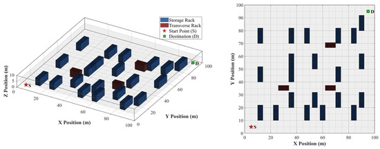
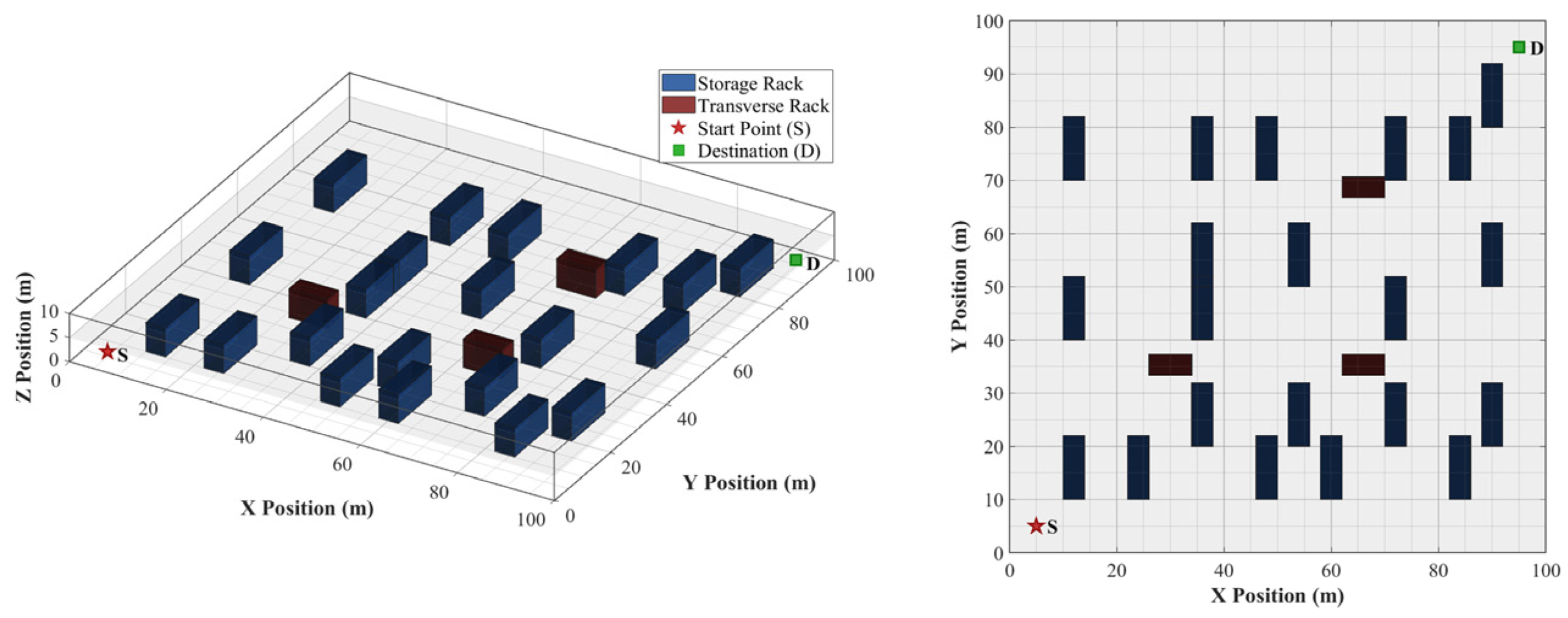
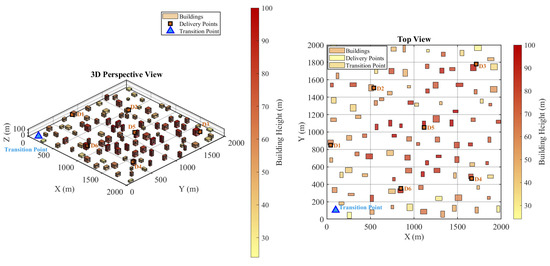
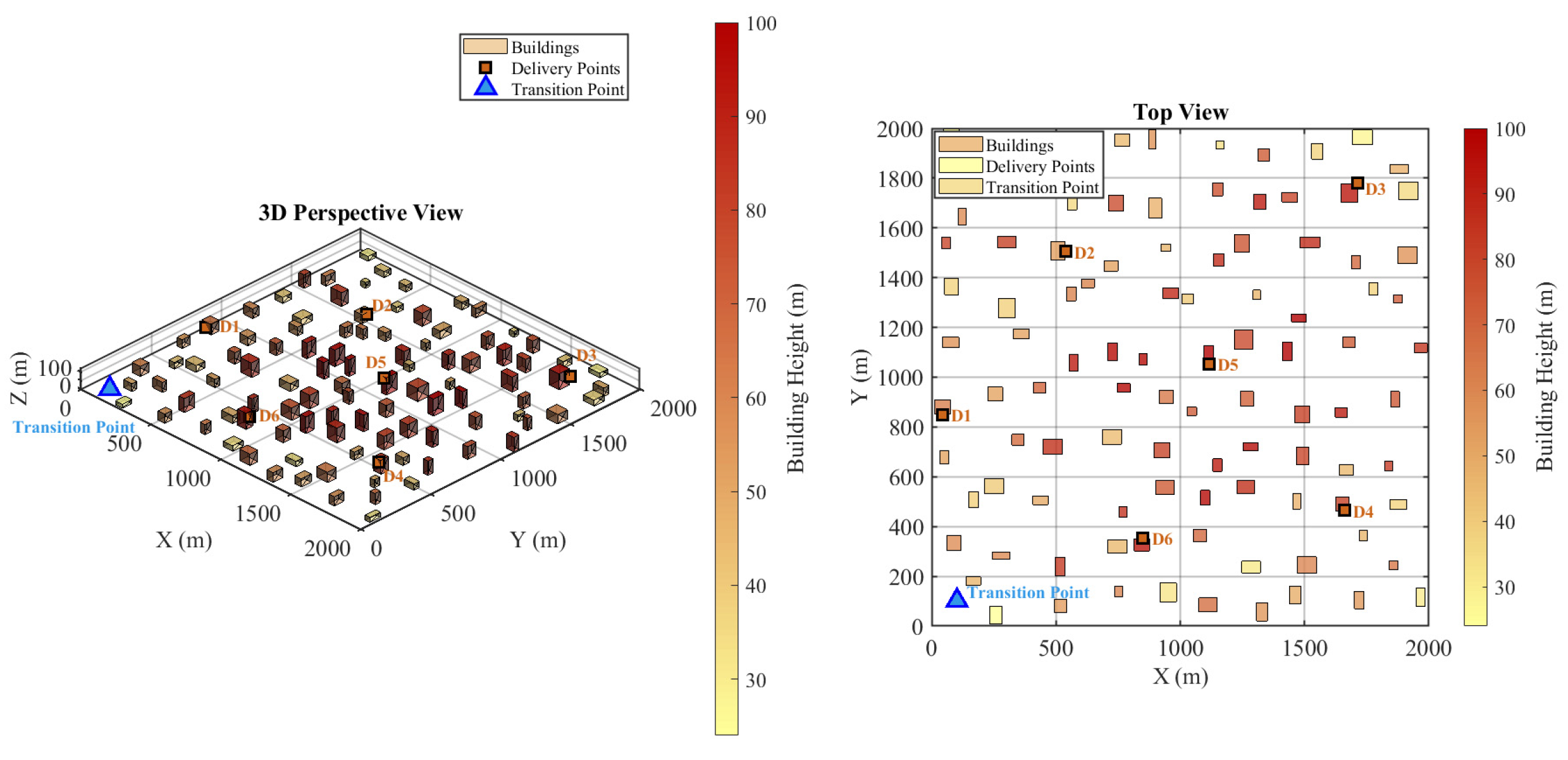
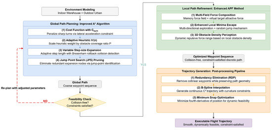
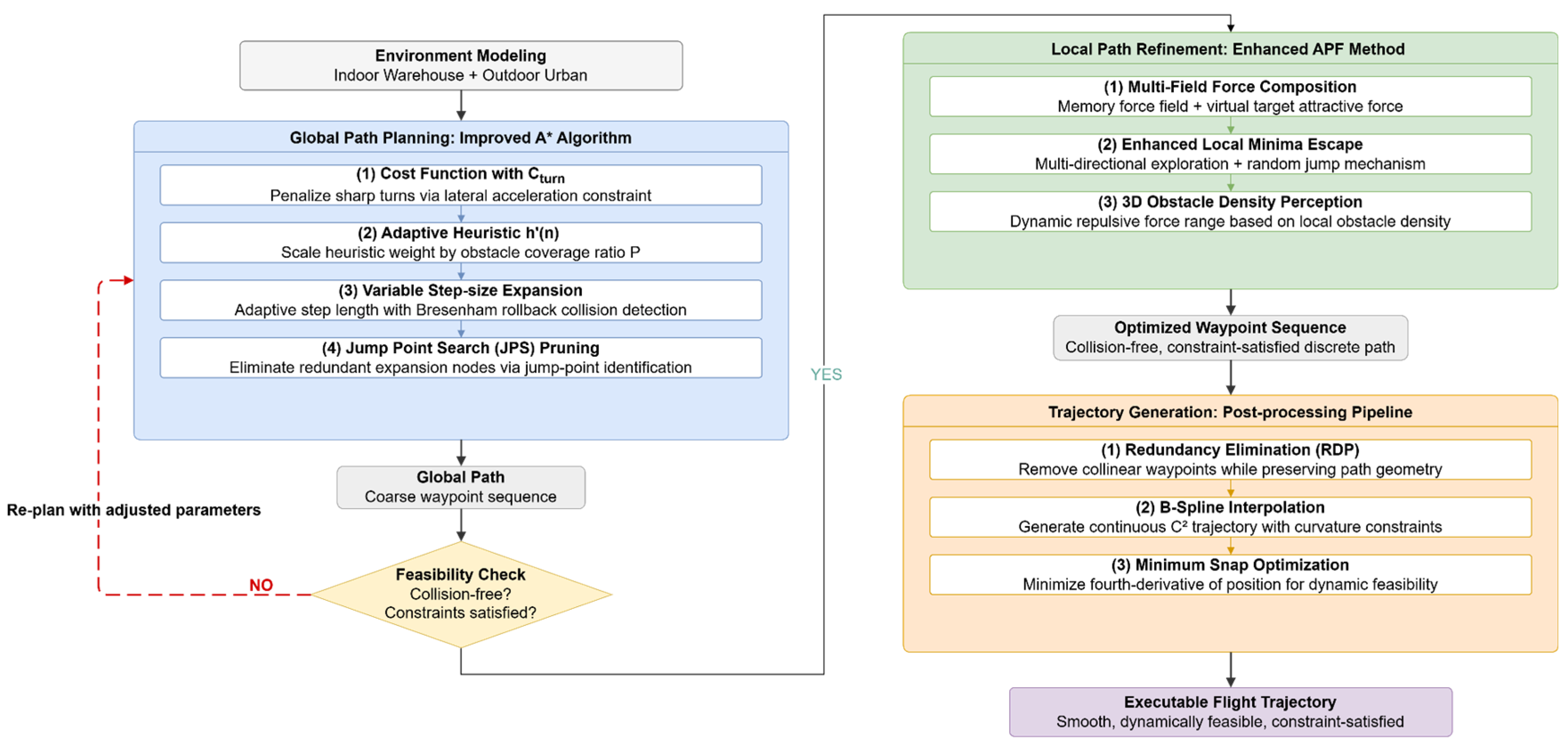
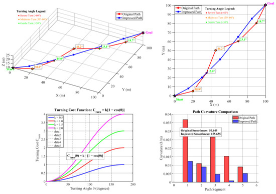
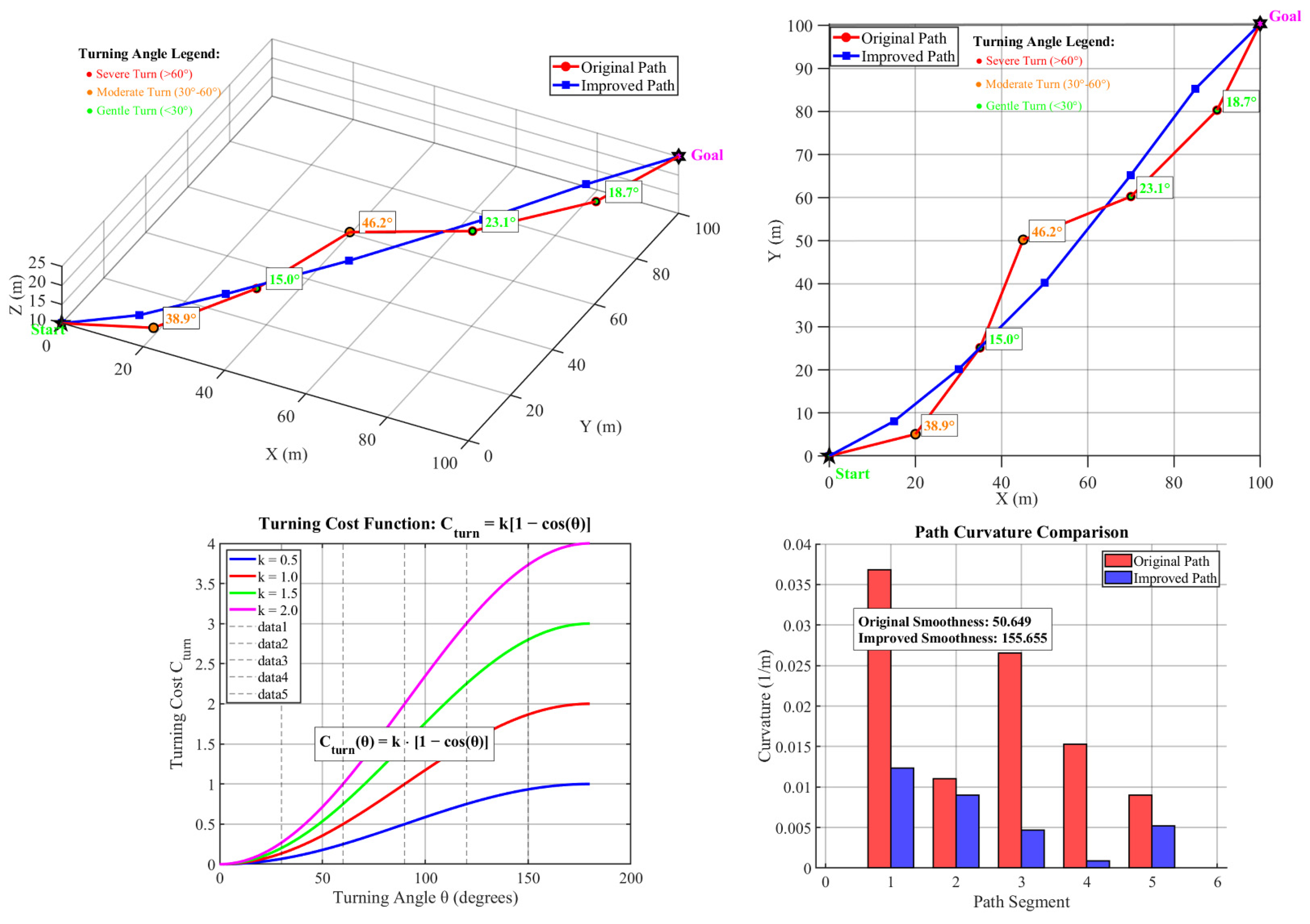
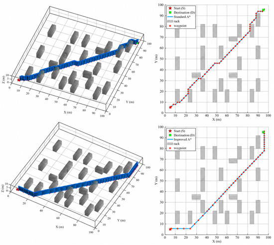
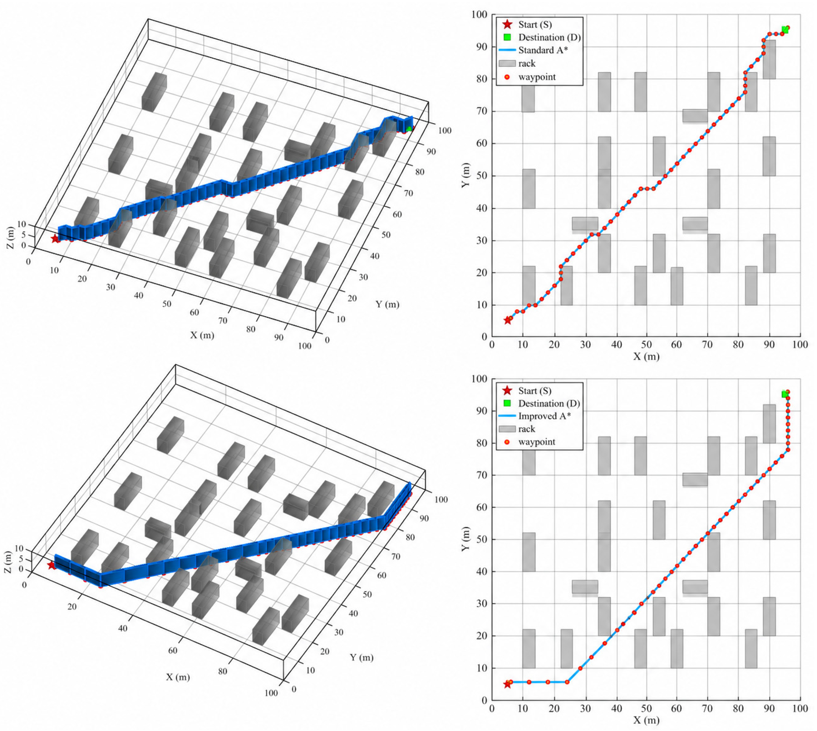
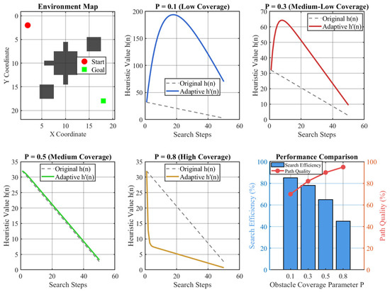
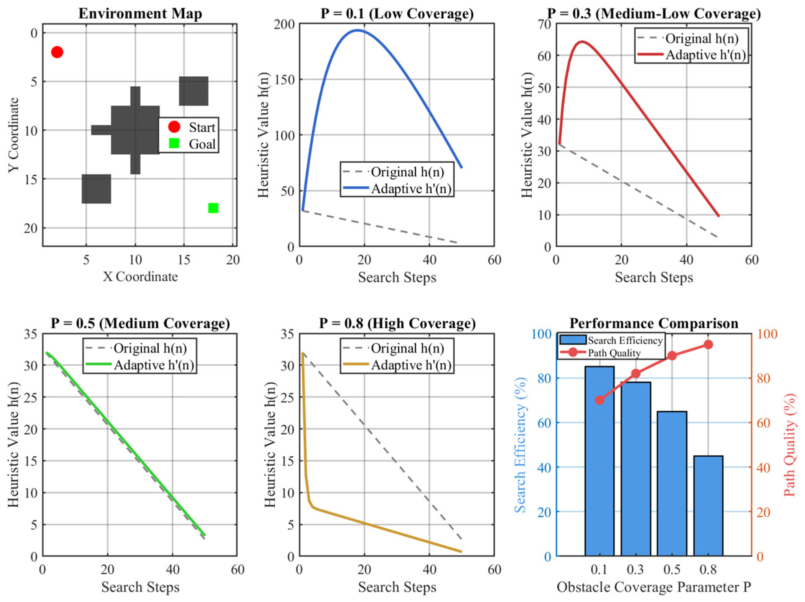
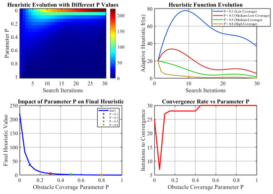
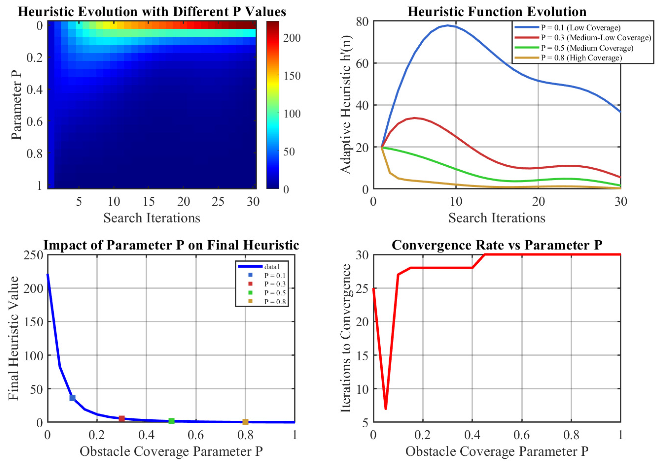
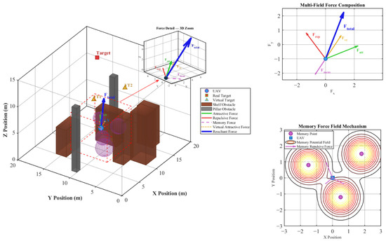
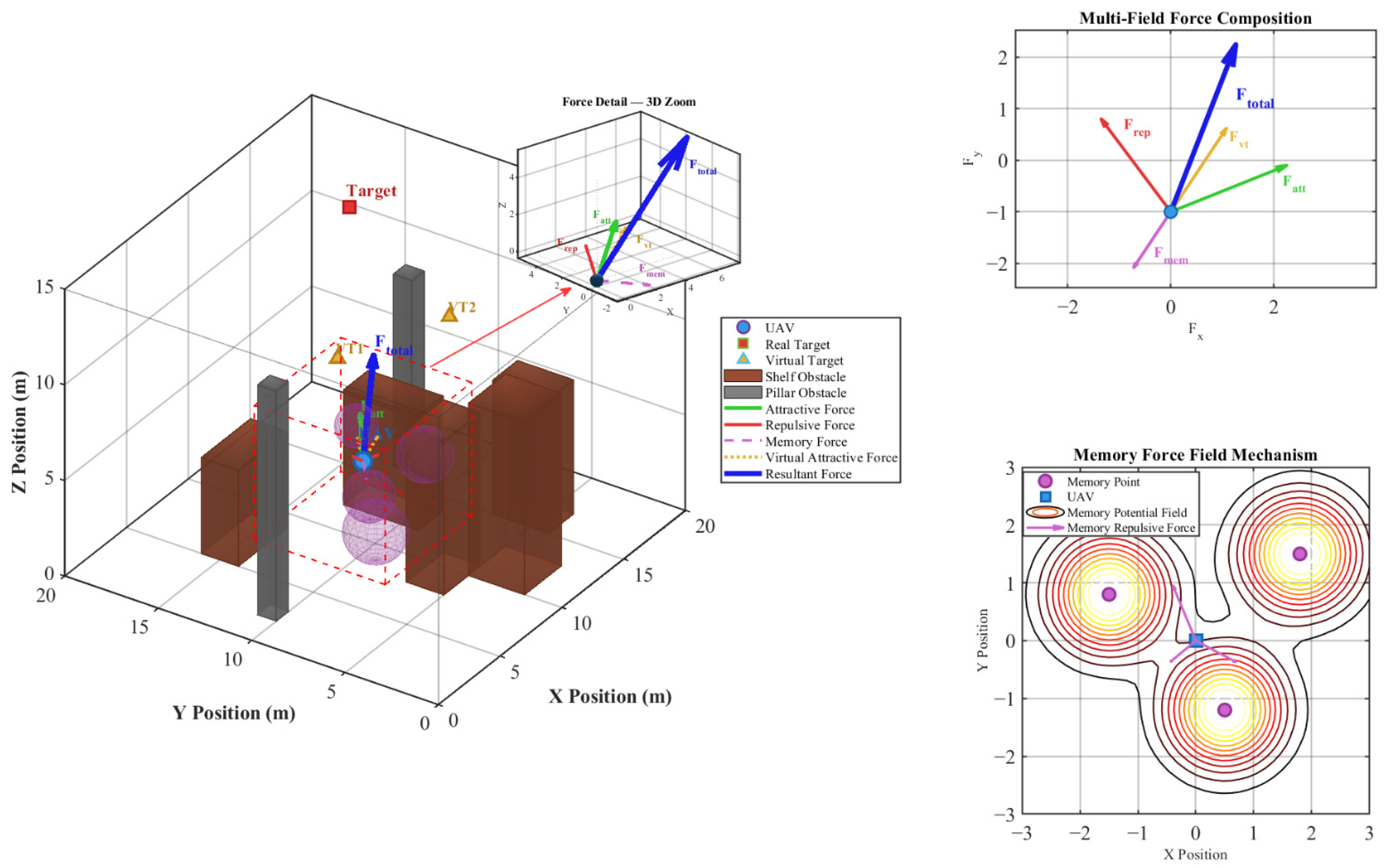
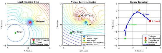
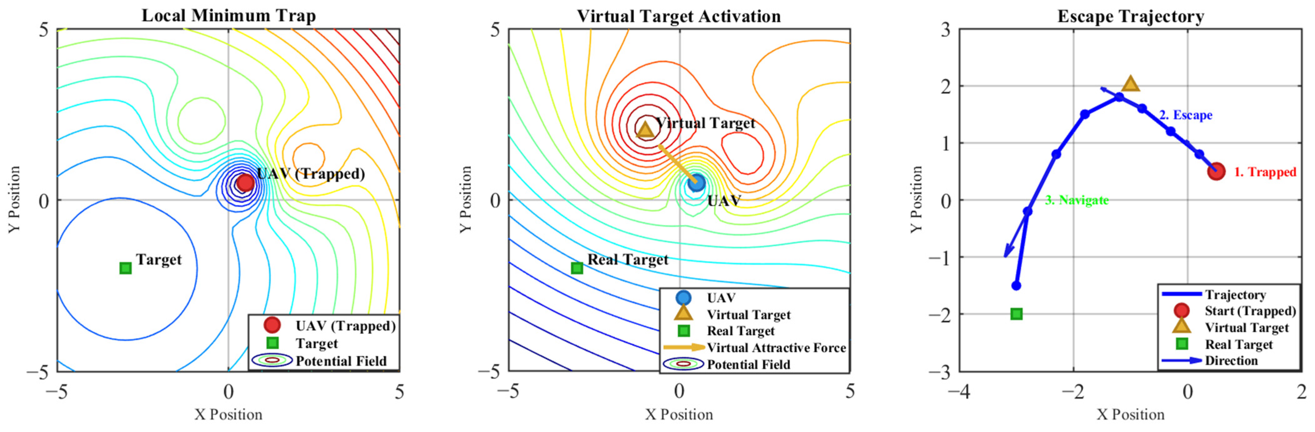
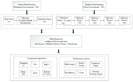
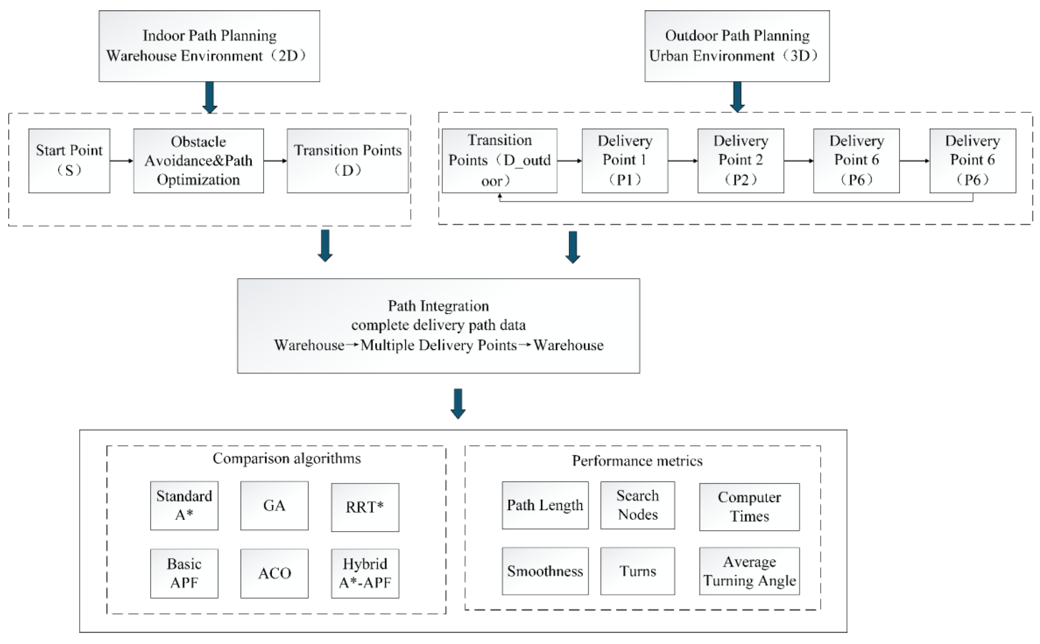
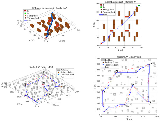
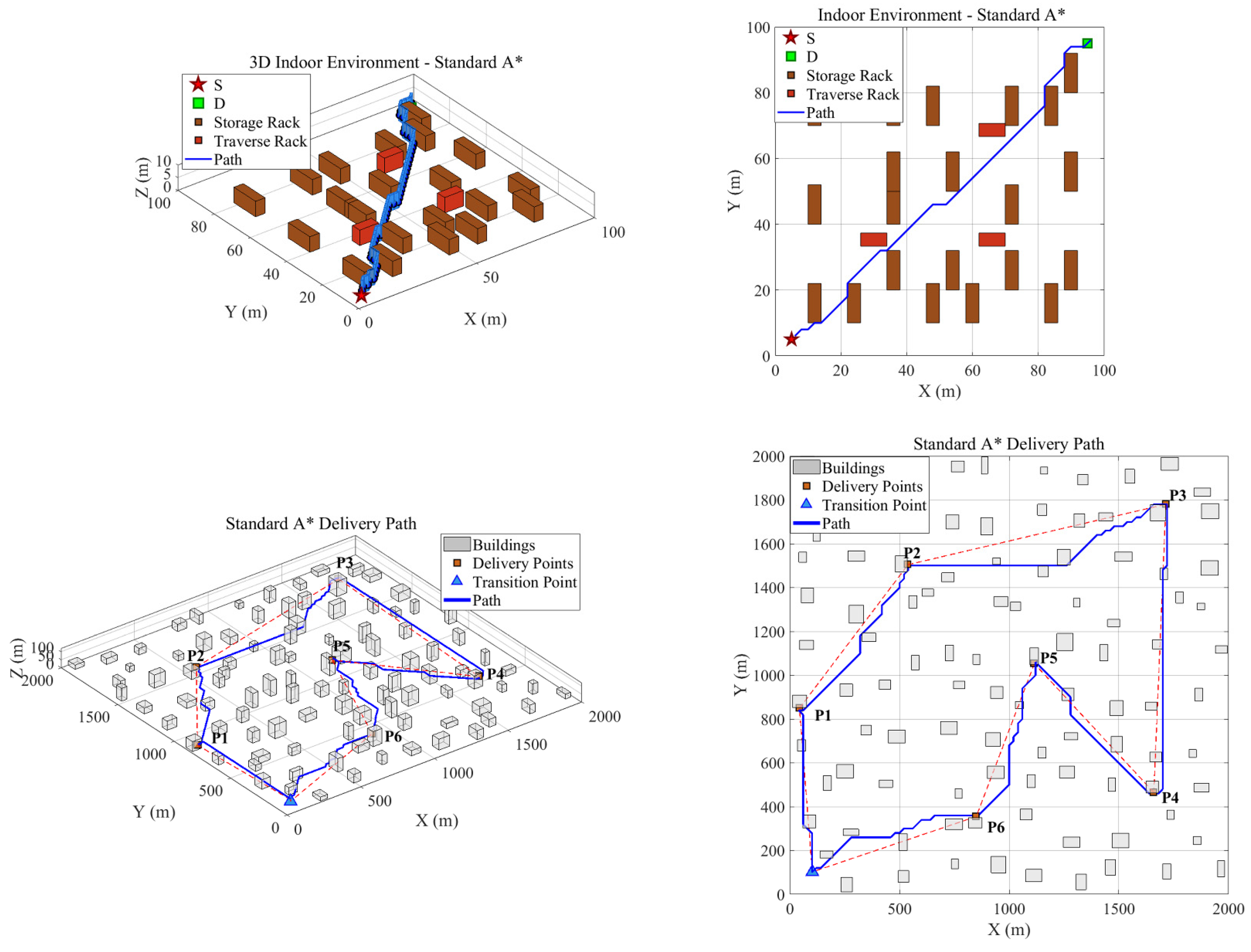
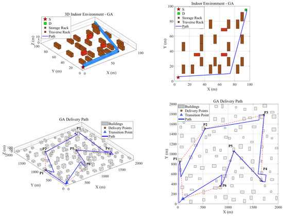
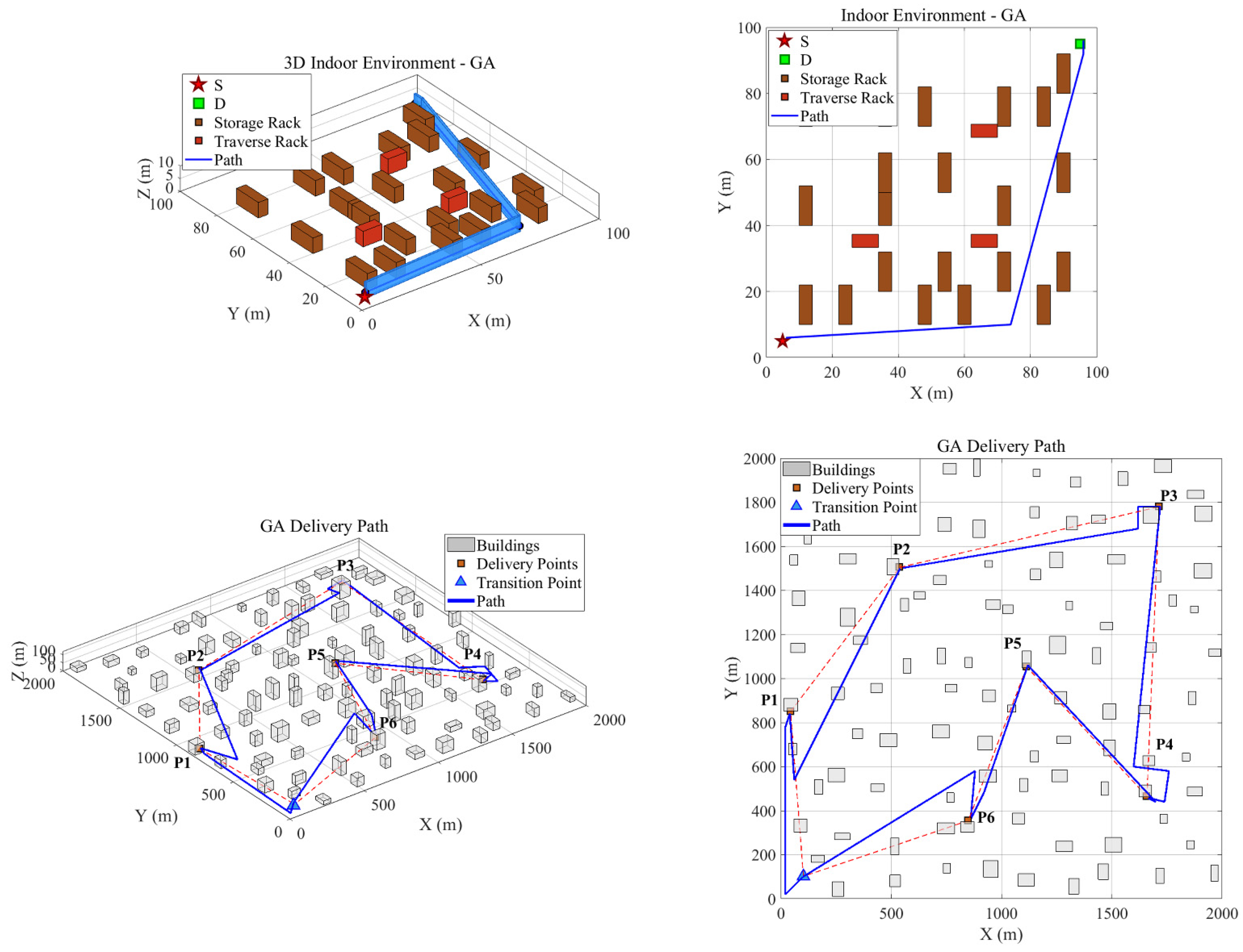
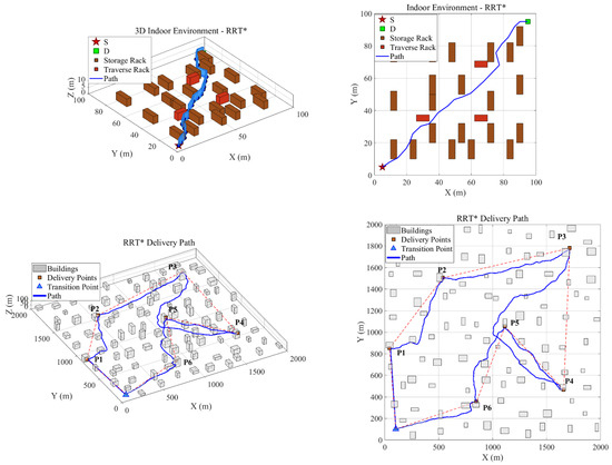
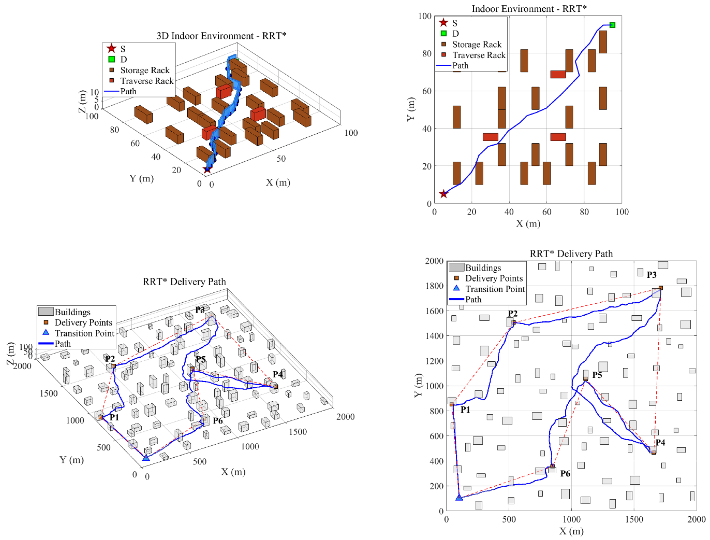
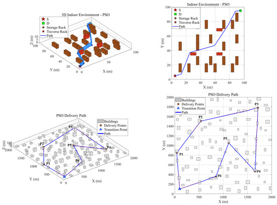
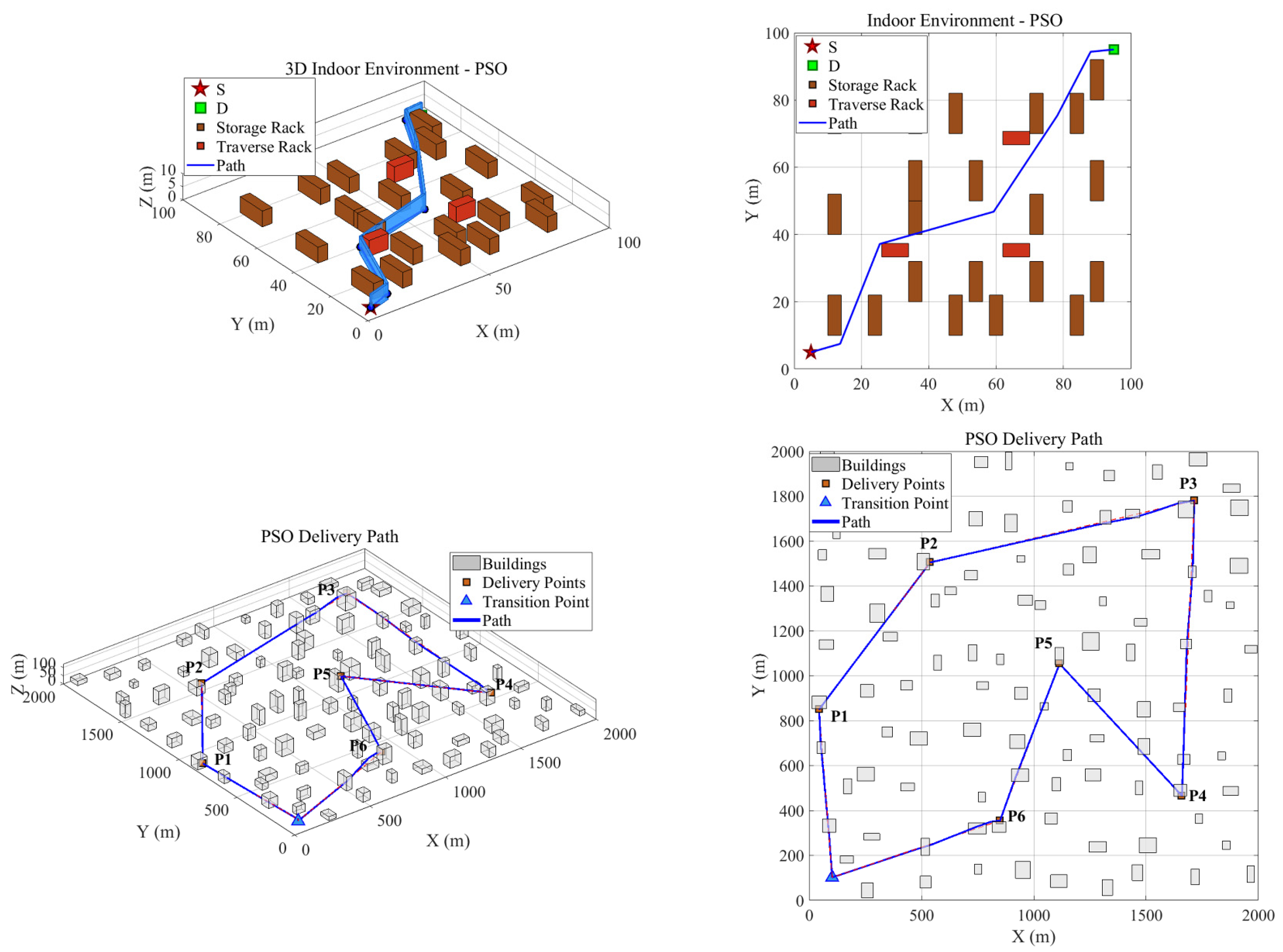
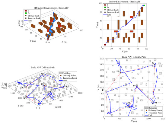
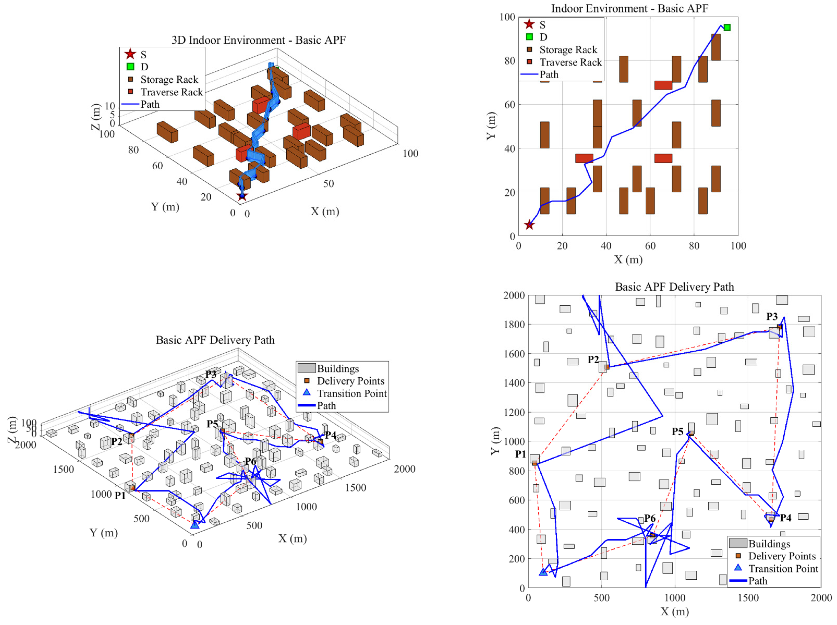
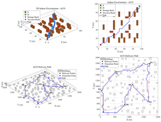
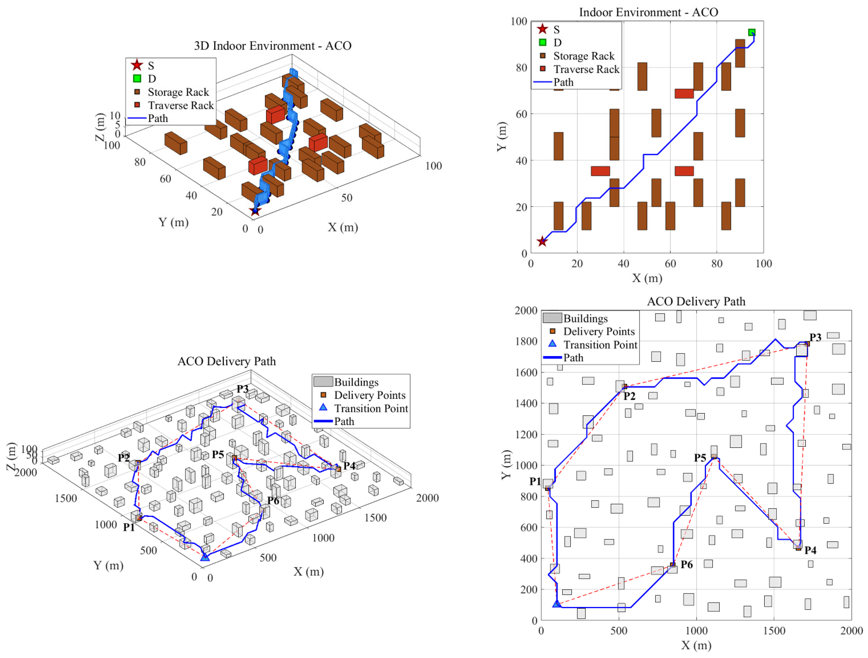
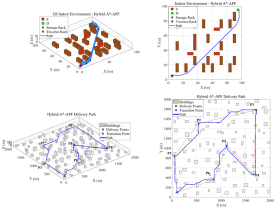
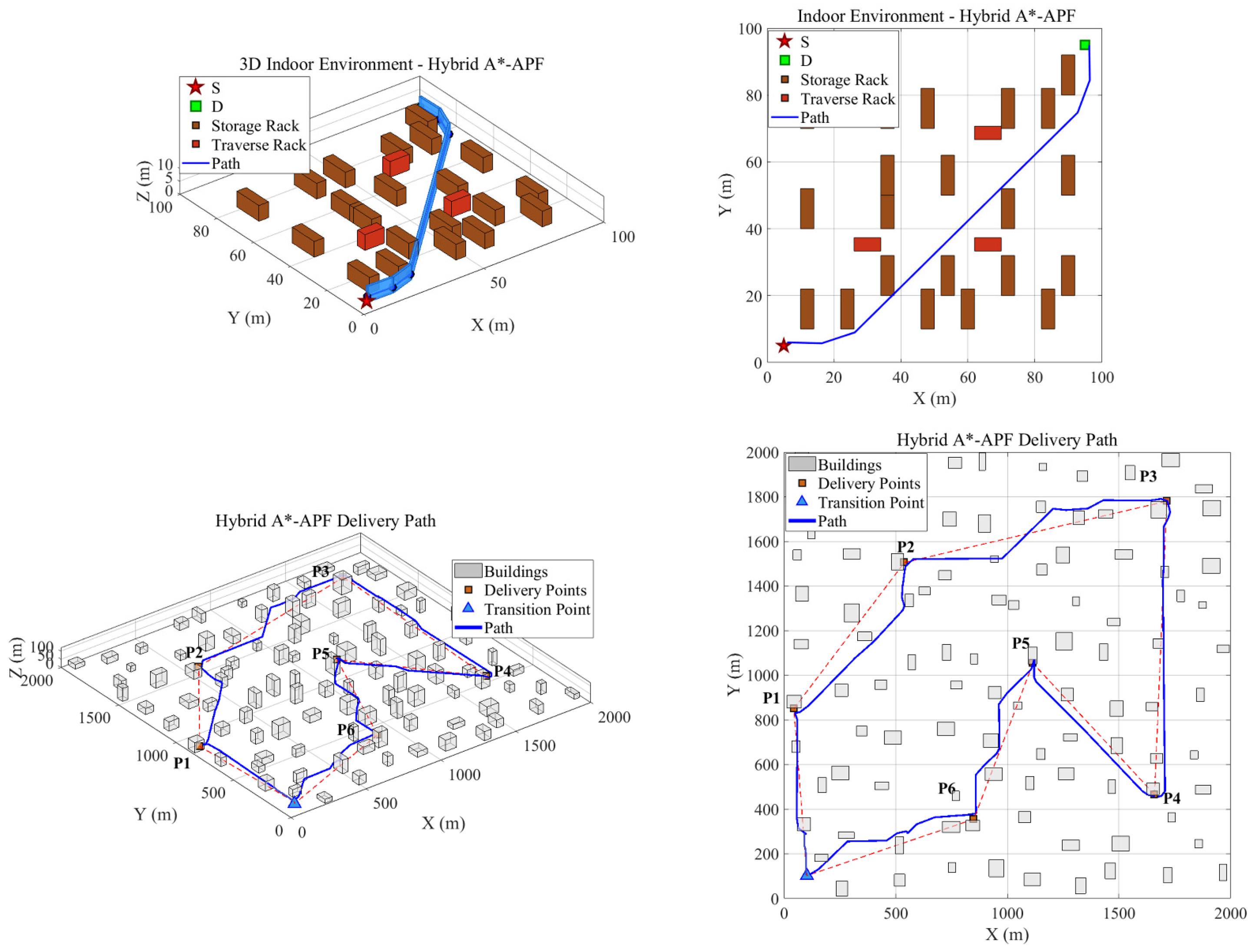
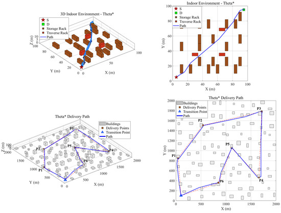
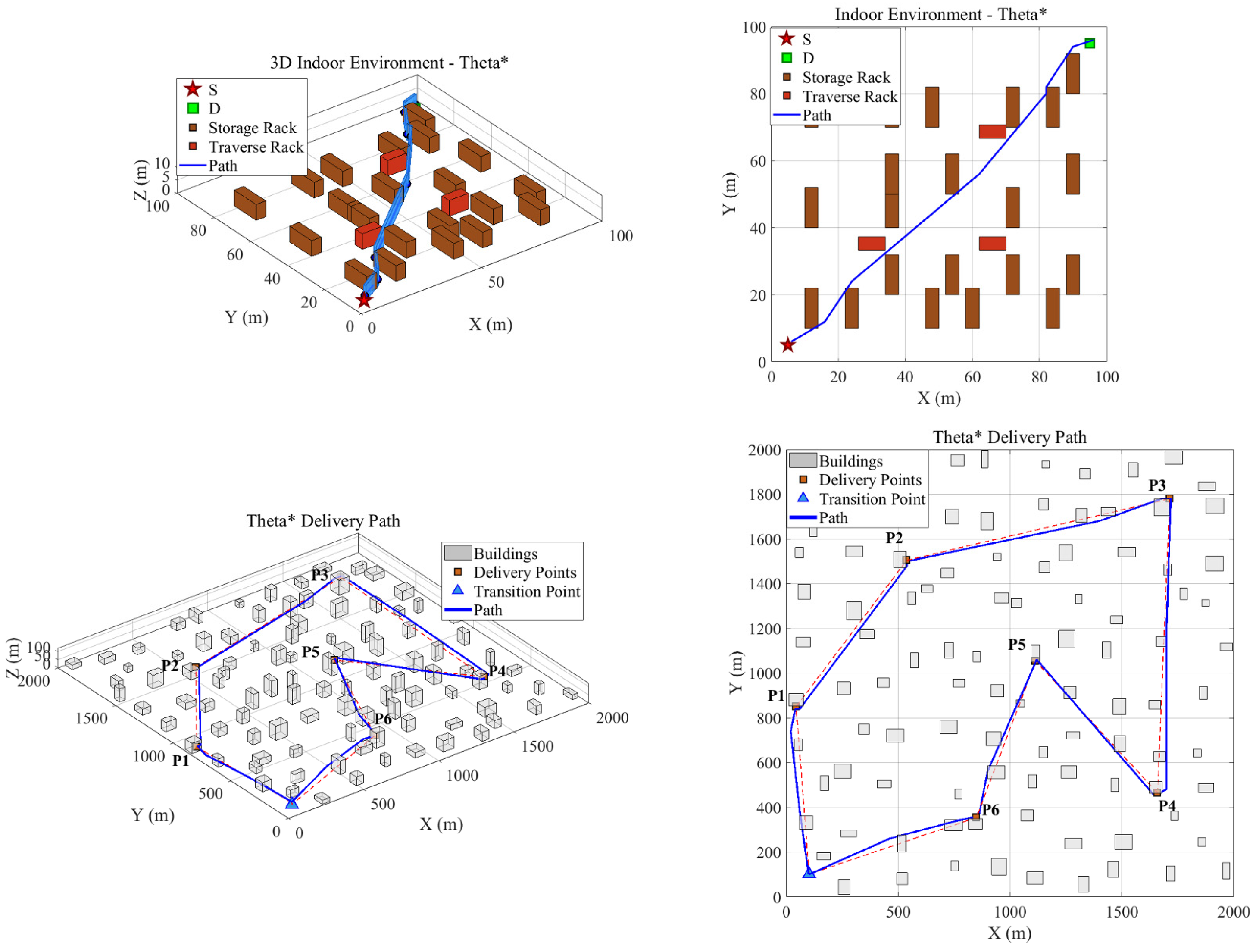
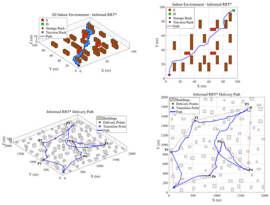
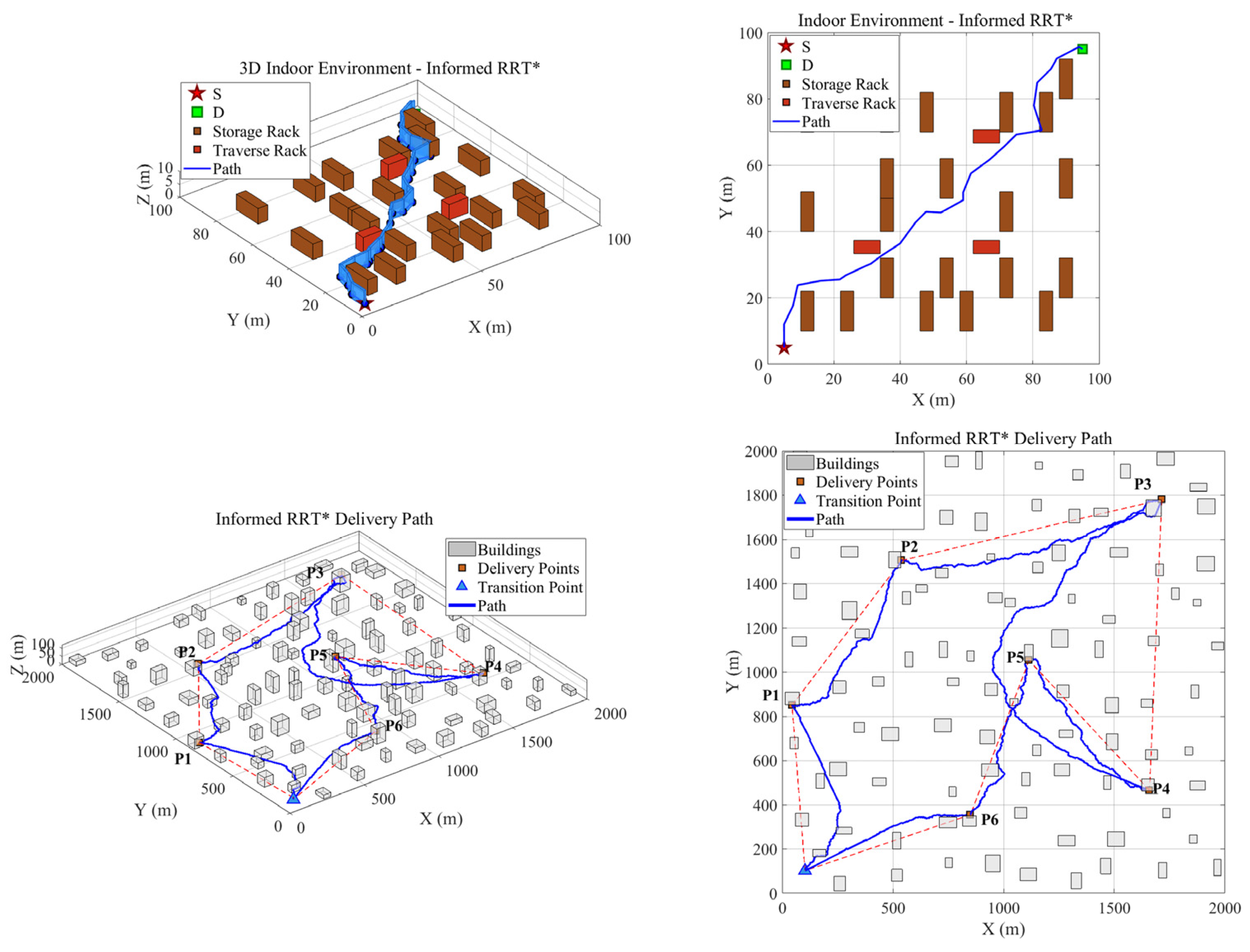
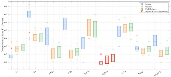
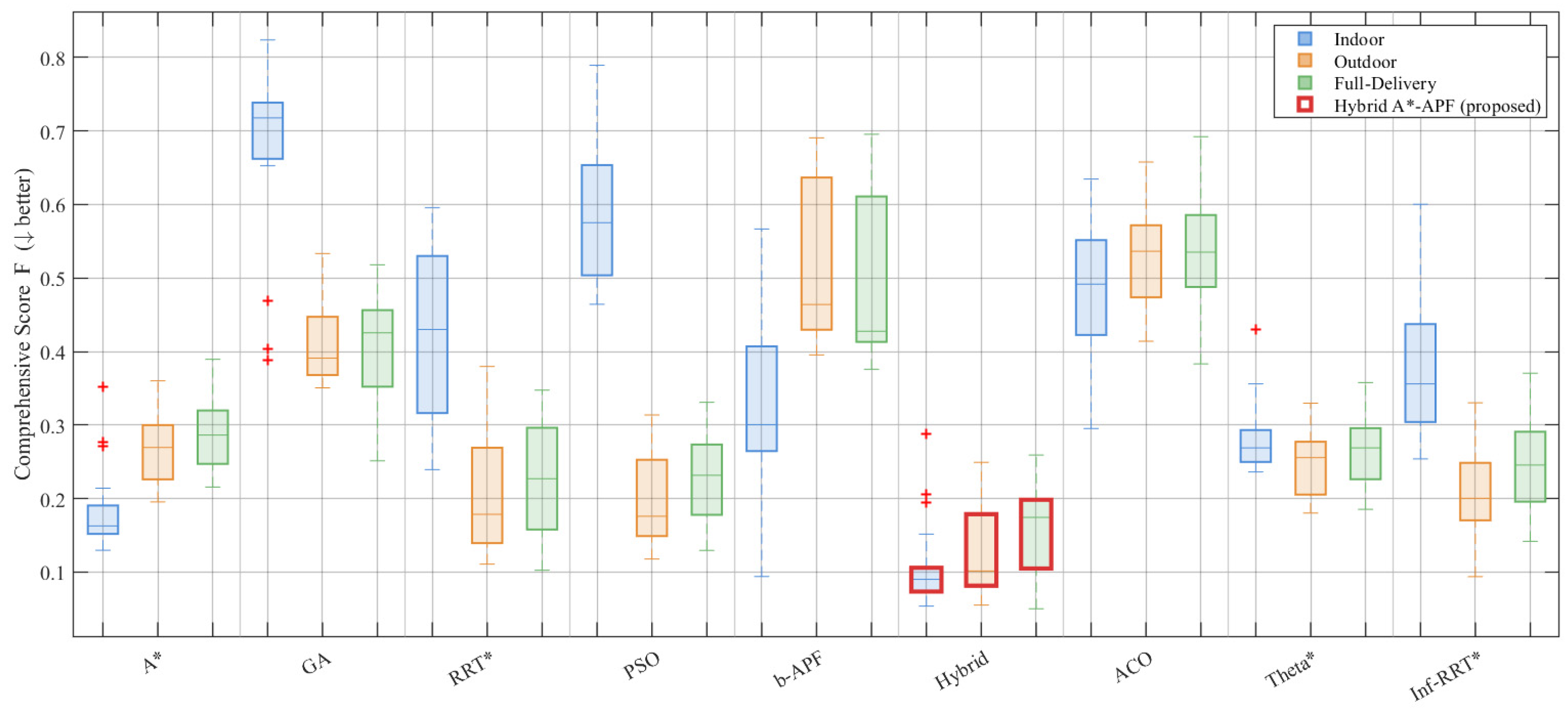
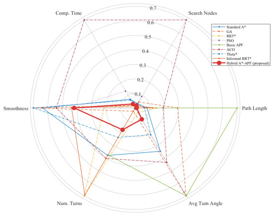
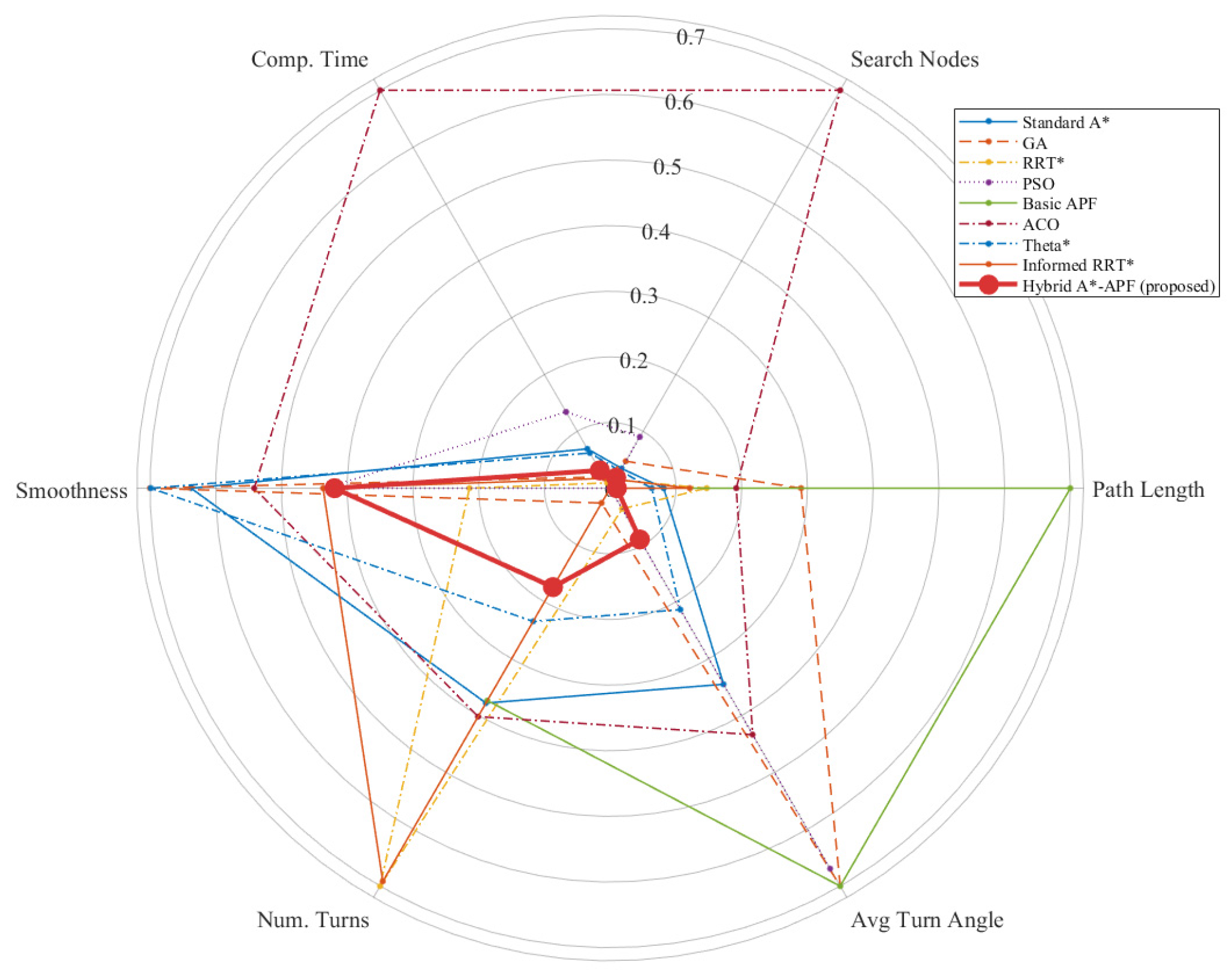
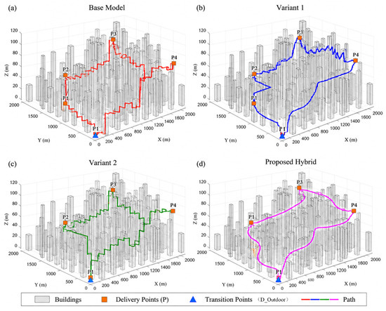
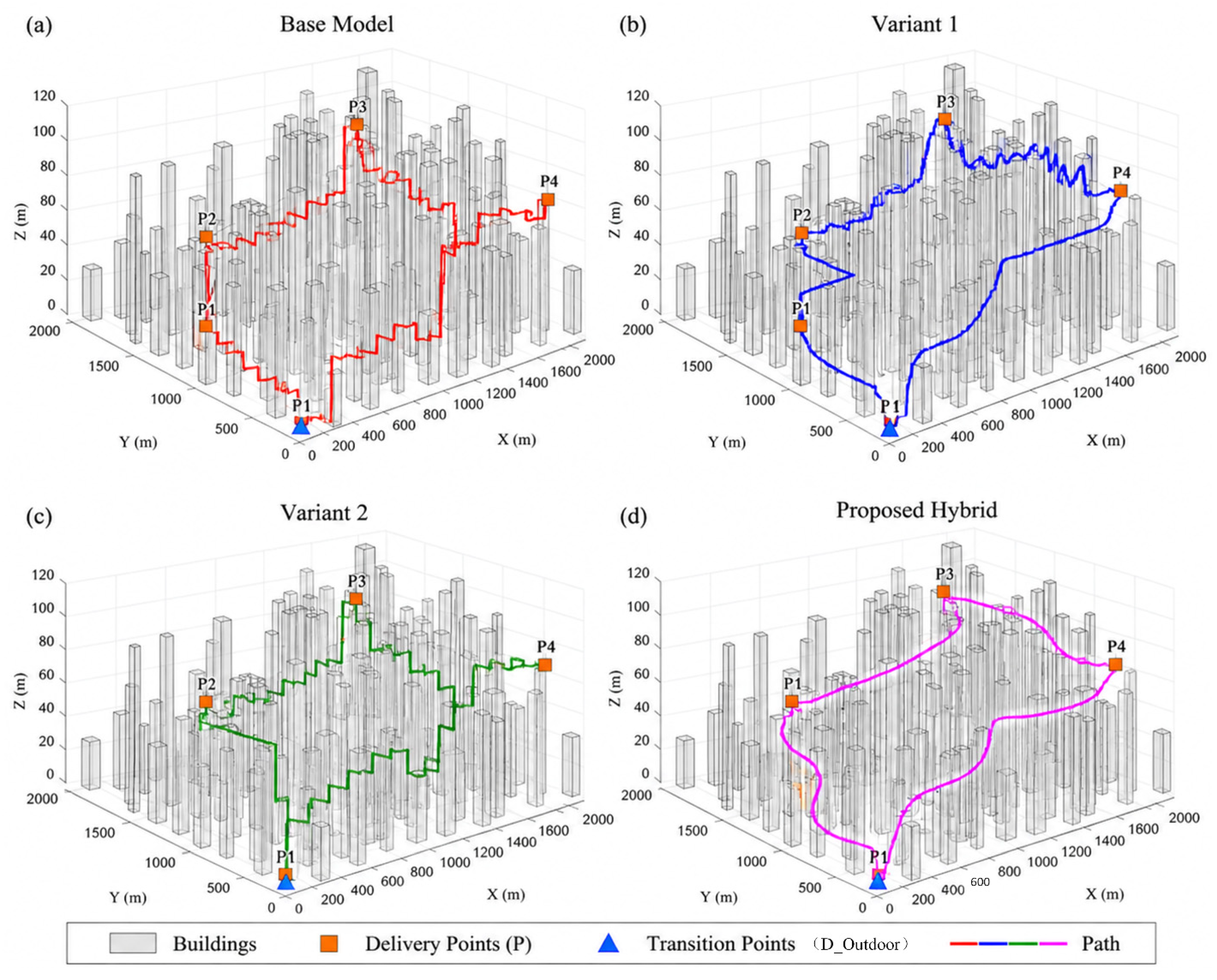
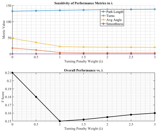
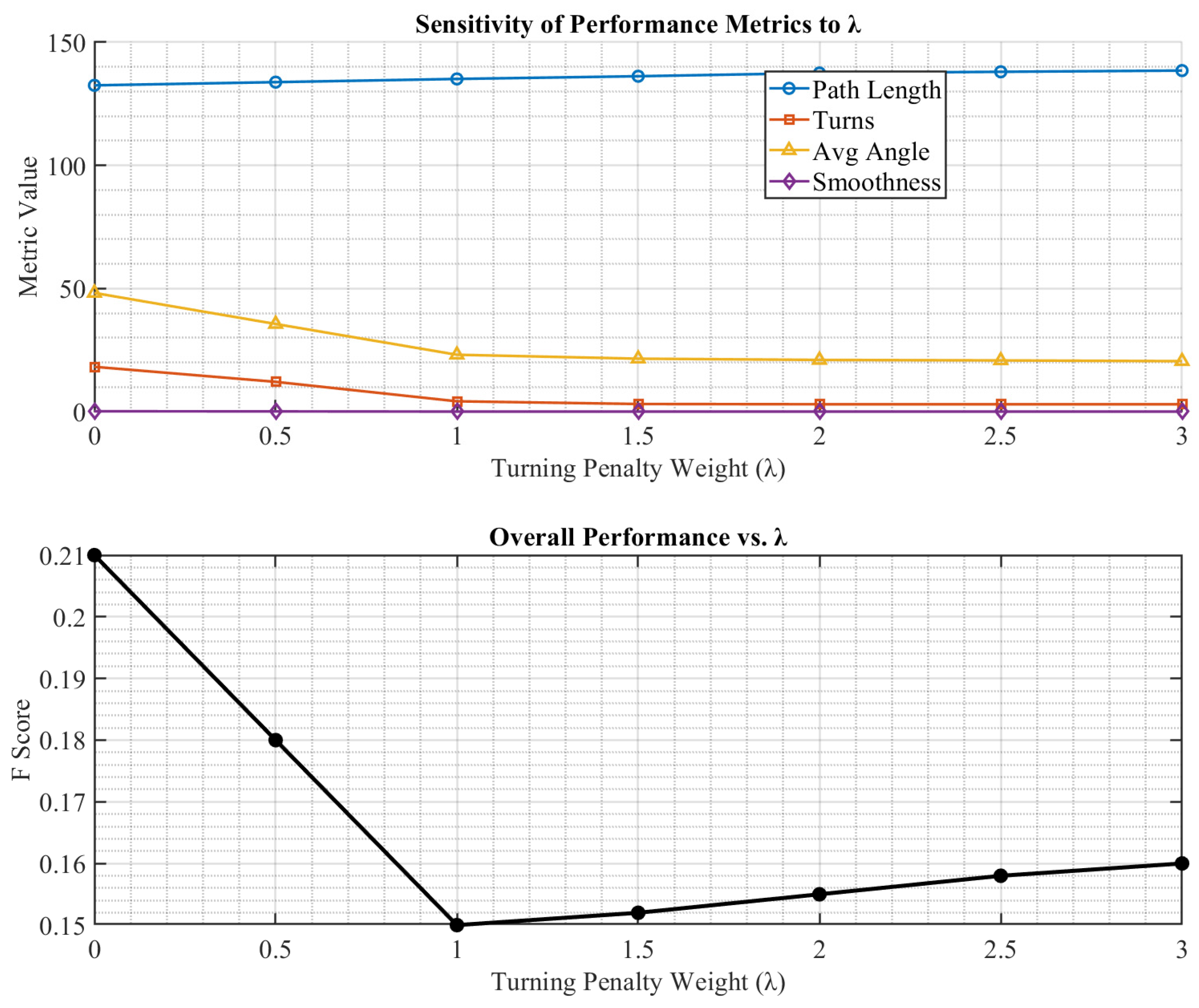
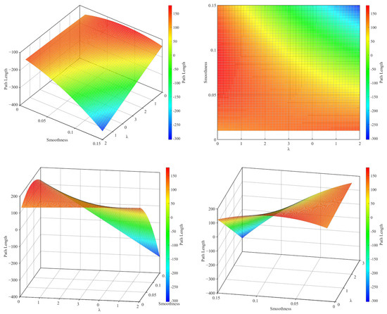
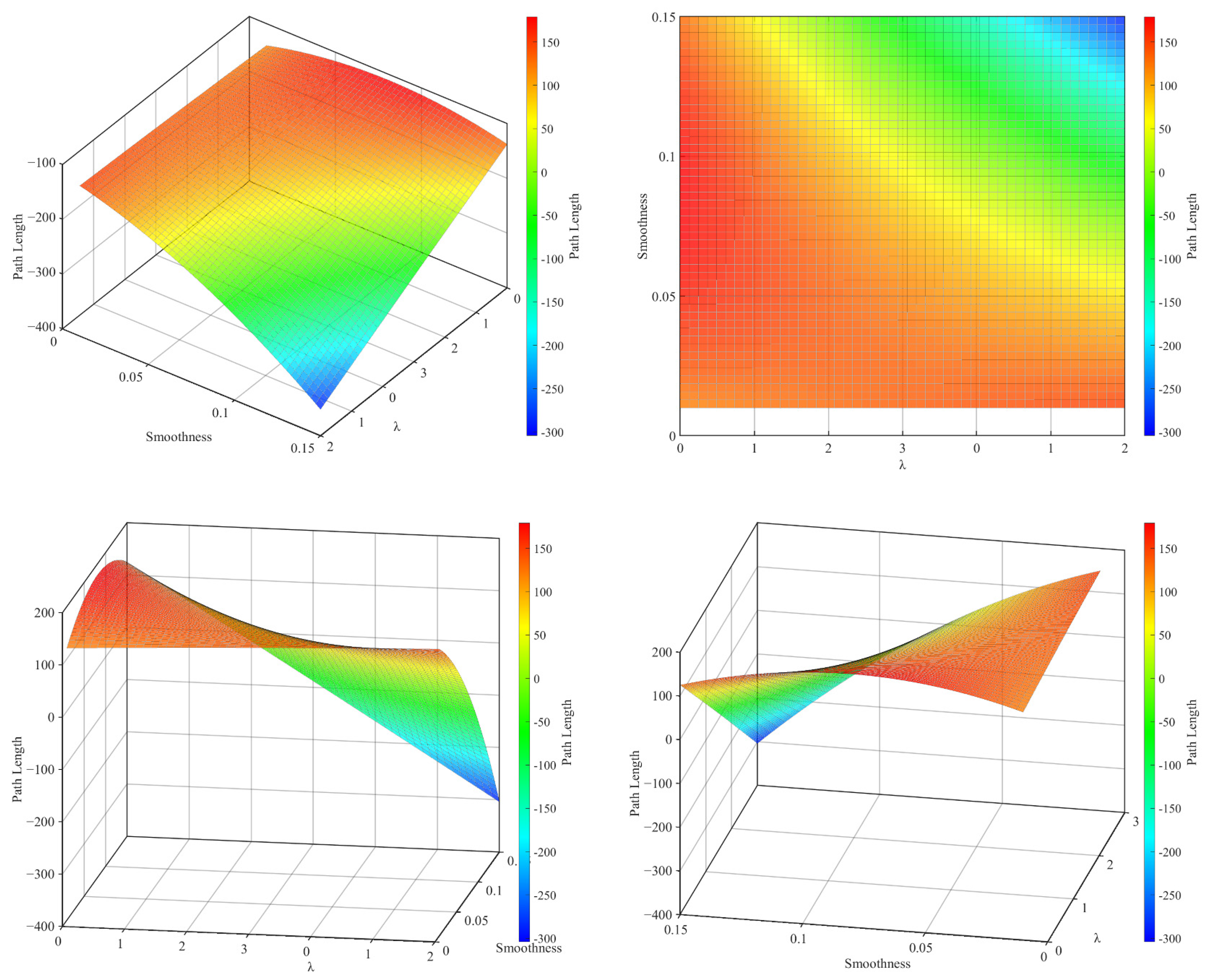
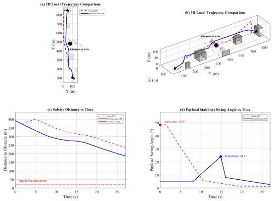
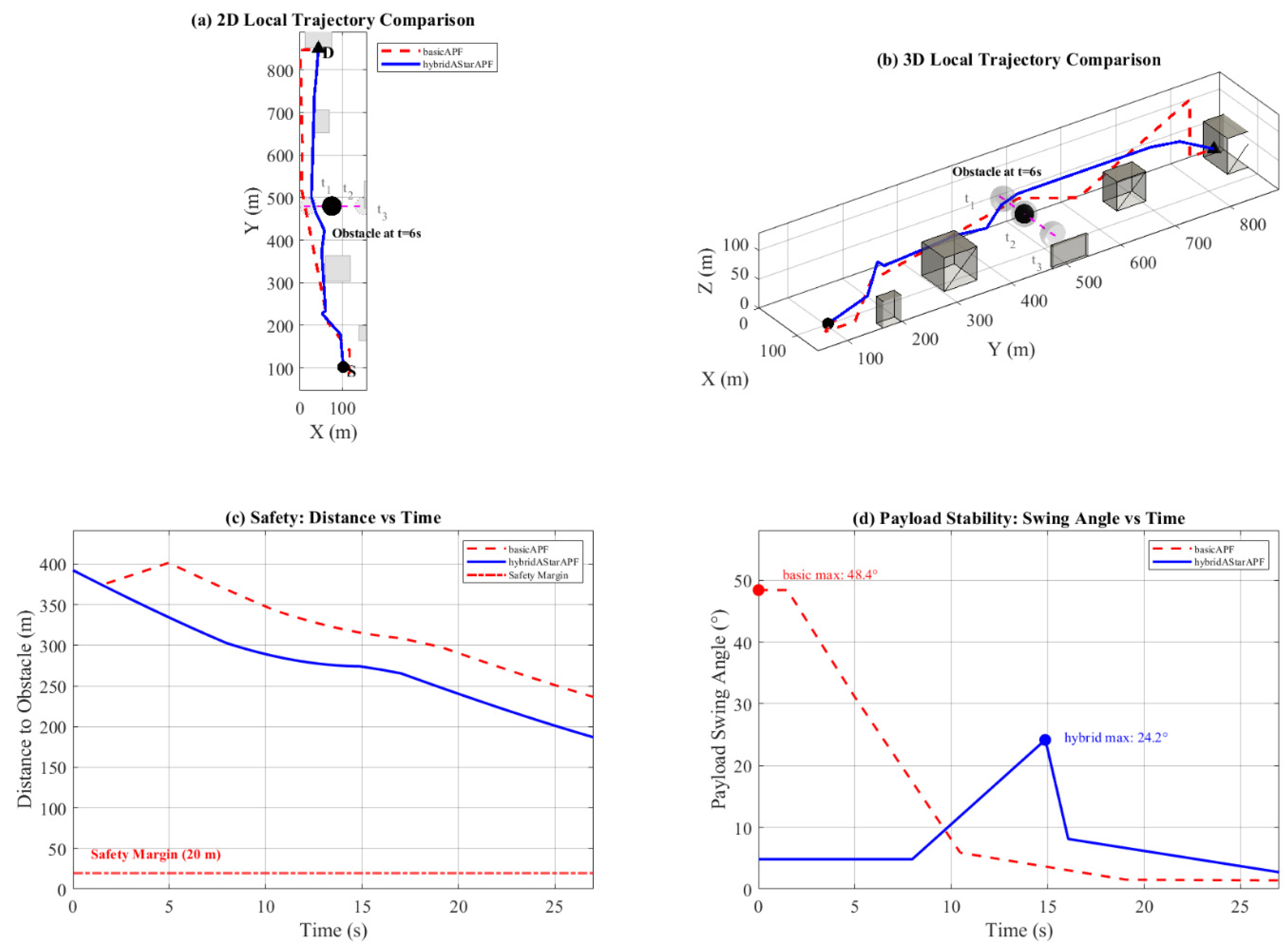
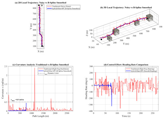
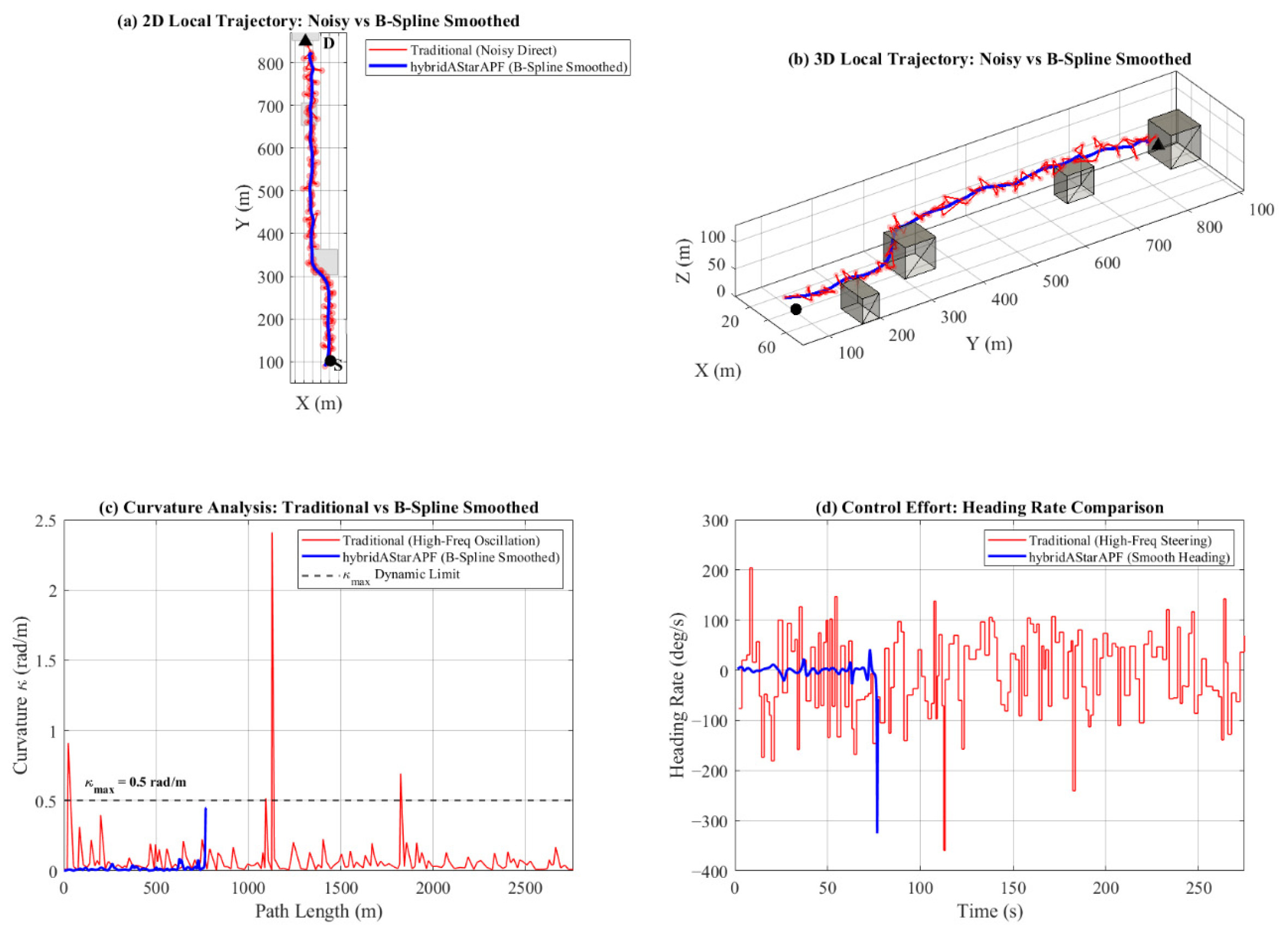
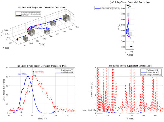
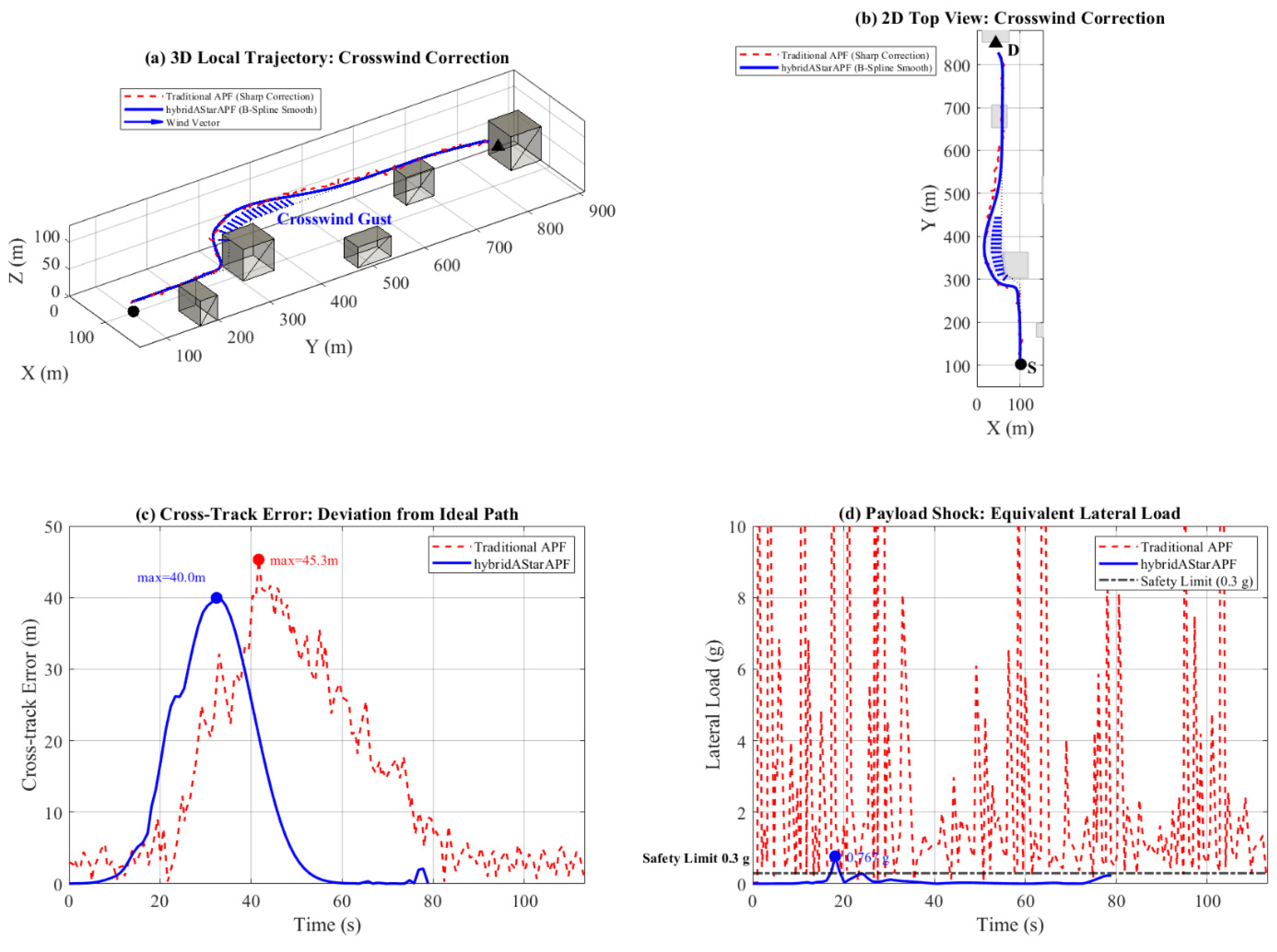

Disclaimer/Publisher’s Note: The statements, opinions and data contained in all publications are solely those of the individual author(s) and contributor(s) and not of MDPI and/or the editor(s). MDPI and/or the editor(s) disclaim responsibility for any injury to people or property resulting from any ideas, methods, instructions or products referred to in the content. |
© 2026 by the authors. Licensee MDPI, Basel, Switzerland. This article is an open access article distributed under the terms and conditions of the Creative Commons Attribution (CC BY) license.