Enhanced Incremental Nonlinear Dynamic Inversion with Aerodynamic Angular Rate Feedback for Autonomous Wing Rock Recovery of a Flying-Wing UAV

Highlights

What are the main findings?

• This study proposes, for the first time, the introduction of aerodynamic angular rate feedback in flight control. The proposed Enhanced Incremental Nonlinear Dynamic Inversion (EINDI) framework, incorporating aerodynamic angular rate feedback into the outer-loop control, achieves successful wing rock recovery from all tested initial states along the limit cycle trajectory.
• Under nominal conditions, EINDI exhibits control accuracy comparable to nonlinear dynamic inversion (NDI)-based control and outperforms linear outer-loop strategies; in the presence of aerodynamic model uncertainties, EINDI maintains superior angle-of-attack tracking accuracy and better sideslip suppression than both NDI-based and linear methods.

What are the implications of the main findings?

• Aerodynamic angular rate feedback offers a viable alternative to model-based control for highly nonlinear flight regimes, reducing reliance on accurate onboard aerodynamic models for wing rock recovery. In addition, the EINDI method is applicable to fixed-wing unmanned aerial platforms equipped with aerodynamic-angle sensing.
• The results reveal that while the attitude control loop possesses strong inherent robustness, the choice of outer-loop architecture significantly affects angle-of-attack regulation accuracy under model uncertainty, providing guidance for controller design in high-maneuverability UAVs.

Abstract

Wing rock motion observed in low-aspect-ratio flying-wing unmanned aerial vehicles (UAVs) severely degrades maneuverability and flight safety, making effective recovery control a challenging task. This paper proposes an Enhanced Incremental Nonlinear Dynamic Inversion (EINDI) control framework for autonomous wing rock recovery, in which aerodynamic angular rate feedback is introduced into the outer-loop control design, while an INDI scheme is employed in the inner loop. The proposed controller is evaluated using a six-degree-of-freedom (6-DOF) flying-wing UAV model. Recovery performance is assessed for multiple initial conditions distributed along the wing rock trajectory, and the results are compared with those obtained using linear outer-loop control, nonlinear dynamic inversion (NDI) outer-loop control, and a simplified NDI-based outer-loop control strategies. Simulation results demonstrate that the proposed method can achieve successful recovery from arbitrary initial states along the wing rock trajectory. It is found that the required recovery altitude exhibits a negative correlation with the Euclidean distance between the initial and target states. Under nominal conditions, the EINDI controller achieves higher control accuracy and better stability than linear outer-loop control and exhibits performance comparable to NDI-based control. In the presence of aerodynamic model uncertainties, the sideslip suppression capability of linear outer-loop control degrades, while the angle-of-attack tracking performance of NDI-based outer-loop control deteriorates. These results indicate that, although the attitude control loop itself possesses strong inherent robustness, the proposed EINDI framework provides improved control accuracy under model uncertainty, making it well suited for high-maneuverability flight control of flying-wing UAVs.

1. Introduction

Advanced unmanned aerial vehicles (UAVs) are increasingly required to achieve high aerodynamic efficiency, large internal volume, and long endurance, which place stringent demands on their aerodynamic and structural design. To meet these demands, UAV configuration design has progressively moved toward tailless layouts, which offer reduced wetted area, lower trim drag, improved structural efficiency, and a higher overall lift-to-drag ratio compared with conventional tailed configurations [1,2]. A low-aspect-ratio flying-wing UAV with a single leading edge, a sweep angle of 65°, and a W-shaped trailing edge has been developed as a generic research platform for this class of configurations [3]. Owing to its representative geometry and aerodynamic characteristics, this configuration has been widely adopted as a research platform for studying the aerodynamics and flight dynamics of low-aspect-ratio tailless UAVs [4]. Nevertheless, flying-wing configurations suffer from inherent stability challenges [5]. The absence of a vertical tail renders the UAV directionally statically unstable, preventing the automatic attenuation of sideslip disturbances. Furthermore, the lack of a horizontal tail can lead to the loss of longitudinal stability in certain angle-of-attack regimes, resulting in pitch-up behavior and an increased risk of high-angle-of-attack stall. During flight at high angles of attack, vortex breakdown along the leading edge may induce flow separation, and the interaction between separated flow and vortical structures can trigger undesirable rotational motions, including spin, tumbling, and wing rock. Extensive experimental and theoretical studies have shown that slender UAVs with large sweep angles are particularly susceptible to wing rock motion [6,7,8]. For low-aspect-ratio flying-wing configurations, computational fluid dynamics simulations [4,9] and bifurcation analyses [10] have further demonstrated that wing rock represents a typical mode of motion instability.

The physical mechanism sustaining wing rock motion in low-aspect-ratio flying-wing UAV arises from the interaction between concentrated leading-edge vortices and separated flow [4,11,12]. At high angles of attack and large roll angles, a strong vortex forms on the leeward wing, generating significant vortex lift, while flow separation on the windward wing reduces lift. The resulting lift asymmetry produces a roll-restoring moment, causing the roll angle to reverse after reaching an extreme value. Due to the relatively low roll damping of low-aspect-ratio UAVs, the roll motion overshoots the neutral position and continues toward the opposite side, with the windward and leeward wings alternating. This mechanism gives rise to a sustained oscillatory motion dominated by roll. In practice, wing rock is a six-degree-of-freedom (6-DOF) phenomenon in which roll dynamics are coupled with complex motions in other degrees of freedom. Wing rock constitutes a typical high-angle-of-attack, stall-induced oscillation that severely restricts the maneuvering envelope of the UAV [11], degrades tracking performance [13], and may ultimately lead to loss of control.

Active control techniques have been shown to mitigate or suppress wing rock motion. For autonomous wing rock recovery control, a variety of analytical nonlinear models have been developed to describe the underlying dynamics, typically formulated as nonlinear differential equations. These models are generally of low order, including the classical single-degree-of-freedom roll model [14], as well as second-order [15], third-order [16], and fifth-order models [17].

The control design for wing rock recovery faces two fundamental challenges. First, due to the strongly nonlinear characteristics of wing rock dynamics, conventional linear control methods are generally inadequate. Second, wing rock is accompanied by complex unsteady aerodynamic effects, which inevitably introduce parameter uncertainties, unmodeled dynamics, and external disturbances into analytical models. As a result, effective control strategies are typically required to possess a certain degree of robustness. To address these issues, various robust and adaptive control approaches have been proposed. Representative examples include robust adaptive control with Fourier series-based uncertainty estimation [18], model reference adaptive control with novel adaptive laws [19], as well as implicit reference model-based methods [16], adaptive fuzzy control [20], and L1 adaptive control [21]. In addition, feedback linearization combined with sliding mode control [17], reinforcement learning-based approaches [21,22], and extended state observer-based methods [23] have also demonstrated effectiveness in wing rock recovery.

Over the past decade, Incremental Nonlinear Dynamic Inversion (INDI) has attracted increasing attention due to its reduced reliance on explicit system models, improved disturbance rejection capability, and applicability to non-affine systems [24,25]. By exploiting measured angular accelerations and control surface deflections as feedback variables, INDI requires little model information beyond control effectiveness derivatives during controller synthesis, which endows it with inherent robustness against modeling uncertainties and unmodeled dynamics. As a result, INDI has been successfully applied in UAVs [26], underwater vehicles [27], spacecraft [28], and various power systems [29]. Salahudden developed a decoupled INDI-based control law for UAV spin recovery [30], indicating its potential applicability to other highly nonlinear flight motions. O. Pfeifle proposed a cascaded INDI framework for three-dimensional path-following, in which an NDI-based attitude control loop was designed using trajectory state information, providing useful insights for wing rock recovery control [31]. Nevertheless, the application of INDI to wing rock recovery control has not yet been reported.

Despite these advances, several limitations remain in the recovery control of wing rock motion for low-aspect-ratio flying-wing UAVs. Most existing wing rock models are reduced-order representations with constrained degrees of freedom and are therefore unable to fully capture UAV motion within a 6-DOF framework. Consequently, the effectiveness of control laws designed based on such simplified models has not been sufficiently validated in full 6-DOF dynamics. Moreover, in existing INDI-based frameworks, the attitude control loop commonly relies on linear outer-loop controllers, model-based NDI schemes [32], or trajectory state information [31]. Under conditions of model uncertainty or navigation system degradation, these approaches may experience performance degradation.

To address these limitations, this paper proposes an enhanced INDI (EINDI) control framework that incorporates aerodynamic angular rate feedback. To the authors’ best knowledge, this is the first study to introduce aerodynamic angular rate feedback into flight control design. The proposed controller is validated on a full 6-DOF wing rock dynamic model, demonstrating its effectiveness in wing rock recovery control. Furthermore, the proposed control structure is platform-independent, making it applicable to various unmanned platforms beyond the specific flying-wing configuration studied here.

The remainder of this paper is organized as follows. Section 2 presents the flight dynamic model of the low-aspect-ratio flying-wing UAV and the characteristics of wing rock motion. Section 3 describes the proposed aerodynamic-angular-rate-feedback-based EINDI control design. Section 4 reports numerical simulation results and discusses the control performance. Finally, Section 5 concludes the paper.

2. Wing Rock Flight Dynamics of Flying-Wing

This chapter establishes the 6-DOF model for analyzing wing rock motion. Section 2.1 provides a brief introduction to the low-aspect-ratio flying wing used in this study. Section 2.2 presents the flight dynamic equations and actuator models that constitute the 6-DOF wing rock model. Section 2.3 describes the onset and development of the wing rock motion.

2.1. Description of Flying-Wing

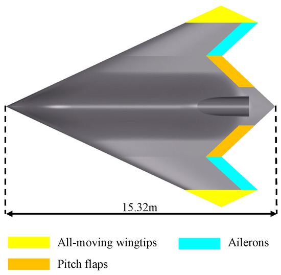
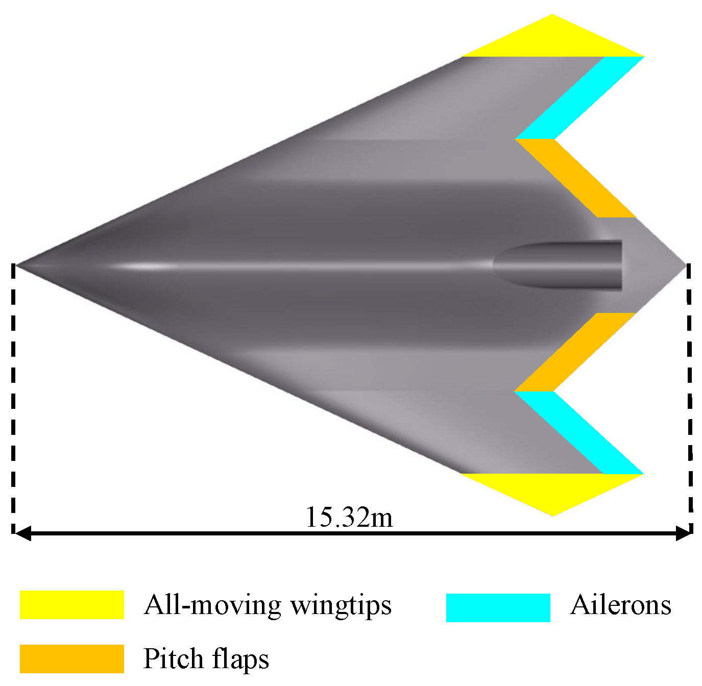
The platform used in this study is a flying-wing UAV, shown in Figure 1, representing a low-aspect-ratio flying-wing configuration developed by the China Aerodynamics Research and Development Center (CARDC). The UAV model has a total length of 15.32 m and a wingspan of 11.43 m, with a large sweep angle of 65° and a small aspect ratio of 1.54. The model parameters are listed in Table 1. Compared with conventional tailed configurations, this flying-wing layout offers a higher lift-to-drag ratio, larger internal volume, and improved structural efficiency, making it a representative platform for studying the aerodynamics and flight dynamics of low-aspect-ratio tailless UAVs. The mass of this flying-wing model is set to 14,855 kg, consistent with that of a geometrically similar tailless configuration reported in [33], owing to their close resemblance in planform layout and aerodynamic characteristics.

Figure 1. Low-aspect-ratio flying-wing UAV model.

Table 1. Model parameters of flying-wing UAV.

Symbol	Parameter	Value	Unit
m	Mass of UAV	14,855	$\mathrm{kg}$
g	Gravitational acceleration	9.765	$\mathrm{m}/{\mathrm{s}}^2$
c	Mean aerodynamic chord	9.56	$\mathrm{m}$
S	Reference wing area	84.6	${\mathrm{m}}^2$
b	Wingspan	11.43	$\mathrm{m}$
A	Aspect ratio	1.54	$\mathrm{m}$
$\rho$	Air density	0.7361	$\mathrm{kg}·{\mathrm{m}}^3$
$I_x$	Moment of inertia about x-axis	48,103	$\mathrm{kg}·{\mathrm{m}}^2$
$I_y$	Moment of inertia about y-axis	106,365	$\mathrm{kg}·{\mathrm{m}}^2$
$I_z$	Moment of inertia about z-axis	149,990	$\mathrm{kg}·{\mathrm{m}}^2$
$I_{xz}$	Product of inertia about x- and z-axes	−712	$\mathrm{kg}·{\mathrm{m}}^2$
$T_{max}$	Maximum thrust of UAV	148,550	$\mathrm{N}$

To address the inherent yaw instability of the flying wing, the UAV utilizes differential drag generated by all-moving wing tips for yaw control. The all-moving wing tip is regarded as a highly effective control effector for flying-wing configurations, as it can provide substantial yawing moments across a wide range of angles of attack. In addition, the inboard elevons are symmetrically deflected to perform pitch control, while the outboard elevons are differentially deflected to realize roll control. In this paper, the terms “elevator,” “rudder,” and “aileron” refer to nominal control quantities with equivalent functions rather than conventional control surfaces on traditional UAVs.

All aerodynamic data from the present model were derived from wind tunnel tests conducted at CARDC, while the inertial data were taken from the geometrically similar configuration reported in [33]. Further modeling details of the present model can be found in our previous work [10].

2.2. Mathematical Model of Flying Wing

2.2.1. Flight Dynamic Equations

From the perspective of flight dynamics, when elastic deformation and other flexible effects of the UAV are neglected, the vehicle can be modeled as a single rigid body. Under this assumption, the rigid-body flight dynamics can be described by a set of differential equations, as given in Equations (1)–(12). This system represents the 6-DOF flight dynamics formulated in the body frame and consists of three force equations (Equations (1)–(3)), three moment equations (Equations (4)–(6)), three velocity equations (Equations (7)–(9)), and three angular rate equations (Equations (10)–(12)). In these equations, $F_x$, $F_y$, and $F_z$, as well as $M_x$, $M_y$, and $M_z$, denote the resultant aerodynamic and propulsive forces and moments acting on the UAV, expressed in the body frame. The complete equation set involves 12 state variables characterizing the UAV’s motion, including the velocity components ${\left[u,v,w\right]}^T$, the angular rate components ${\left[p,q,r\right]}^T$, the position components ${\left[x,y,z\right]}^T$, and the Euler angles ${\left[\varphi ,\theta ,\psi \right]}^T$. The 6-DOF motion described by these 12 equations can be directly implemented using the 6-DOF (Euler Angles) block provided in MATLAB/Simulink R2023b.

$$\dot{u}={\displaystyle \frac{F_x}{m}}-qw+rv$$

(1)

$$\dot{v}={\displaystyle \frac{F_y}{m}}-ru+pw$$

(2)

$$\dot{w}={\displaystyle \frac{F_z}{m}}-pv+qu$$

(3)

$$\begin{array}{c}\dot{p}={\displaystyle \frac{I_z{M}_x+I_{xz}{M}_z}{I_x{I}_z-I_{xz}^2}}+{\displaystyle \frac{I_{xz}\left(I_x-I_y+I_z\right)}{I_x{I}_z-I_{xz}^2}}pq+{\displaystyle \frac{I_y{I}_z-I_z^2-I_{xz}^2}{I_x{I}_z-I_{xz}^2}}qr\end{array}$$

(4)

$$\dot{q}={\displaystyle \frac{M_y}{I_y}}+{\displaystyle \frac{I_z-I_x}{I_y}}pr+{\displaystyle \frac{I_{xz}}{I_y}}\left(r^2-p^2\right)$$

(5)

$$\begin{array}{c}\dot{r}={\displaystyle \frac{I_{xz}{M}_x+I_x{M}_z}{I_x{I}_z-I_{xz}^2}}+{\displaystyle \frac{I_x^2+I_{xz}^2-I_x{I}_y}{I_x{I}_z-I_{xz}^2}}pq+{\displaystyle \frac{I_{xz}\left(I_y-I_x-I_z\right)}{I_x{I}_z-I_{xz}^2}}qr\end{array}$$

(6)

$$\begin{array}{c}\dot{x}=u\cos \theta \cos \psi +v\left(\sin \varphi \sin \theta \cos \psi -\cos \varphi \sin \psi \right)+w\left(\cos \varphi \sin \theta \cos \psi +\sin \varphi \sin \psi \right)\end{array}$$

(7)

$$\begin{array}{c}\dot{y}=u\cos \theta \sin \psi +v\left(\sin \varphi \sin \theta \sin \psi +\cos \varphi \cos \psi \right)+w\left(\cos \varphi \sin \theta \sin \psi -\sin \varphi \cos \psi \right)\end{array}$$

(8)

$$\dot{z}=-u\sin \psi +v\sin \varphi \cos \theta +w\cos \varphi \cos \theta$$

(9)

$$\dot{\varphi }=p+\tan \theta ·\left(q\sin \varphi +r\cos \varphi \right)$$

(10)

$$\dot{\theta }=q\cos \varphi -r\sin \varphi$$

(11)

$$\dot{\psi }=\sec \theta \left(q\sin \varphi +r\cos \varphi \right)$$

(12)

In addition to the 12 state variables defined in the above equation set, several other flight states of particular importance can be derived from these variables. Specifically, the angle of attack $\alpha$, sideslip angle $\beta$, and total airspeed V can be computed from the state variables using Equations (13)–(15), respectively.

$$\alpha ={\tan }^{-1}\left({\displaystyle \frac{w}{u}}\right)$$

(13)

$$\beta ={\tan }^{-1}\left({\displaystyle \frac{v}{\sqrt{u^2+w^2}}}\right)$$

(14)

$$V=\sqrt{u^2+v^2+w^2}$$

(15)

The UAV velocity roll angle $\mu$, flight-path angle $\gamma$, and heading angle $\chi$ can be determined from the equivalence relationships among coordinate transformation matrices. Specifically, Equation (16) states that the transformation matrix from the inertial frame to the wind frame is equal to the product of the transformation matrix from the inertial frame to the body frame and that from the body frame to the wind frame.

$$T_{we}=T_{wb}·T_{be}$$

(16)

Here, $T_{we}$ denotes the transformation matrix from the inertial frame to the wind frame, $T_{wb}$ represents the transformation matrix from the body frame to the wind frame, and $T_{be}$ denotes the transformation matrix from the inertial frame to the body frame. The explicit expressions of these three transformation matrices are given in Equations (17)–(19).

$$T_{wb}=\left[\begin{array}{ccc}\cos \alpha \cos \beta & \sin \beta & \sin \alpha \cos \beta \\ -\cos \alpha \sin \beta & \cos \beta & -\sin \alpha \sin \beta \\ -\sin \alpha & 0& \cos \alpha \end{array}\right]$$

(17)

$$T_{be}=\left[\begin{array}{ccc}\cos \theta \cos \psi & \cos \theta \sin \psi & -\sin \theta \\ \sin \theta \sin \varphi \cos \psi -\sin \psi \cos \varphi & \sin \psi \sin \theta \sin \varphi +\cos \psi \cos \varphi & \sin \varphi \cos \theta \\ \sin \theta \cos \varphi \cos \psi +\sin \psi \sin \varphi & \sin \psi \sin \theta \cos \varphi -\cos \psi \sin \varphi & \cos \varphi \cos \theta \end{array}\right]$$

(18)

$$T_{we}=\left[\begin{array}{ccc}\cos \gamma \cos \chi & \cos \gamma \sin \chi & -\sin \gamma \\ \sin \gamma \sin \mu \cos \chi -\sin \chi \cos \mu & \sin \chi \sin \gamma \sin \mu +\cos \chi \cos \mu & \sin \mu \cos \gamma \\ \sin \gamma \cos \mu \cos \chi +\sin \chi \sin \mu & \sin \chi \sin \gamma \cos \mu -\cos \chi \sin \mu & \cos \mu \cos \gamma \end{array}\right]$$

(19)

Based on this equivalence relationship, the velocity roll angle $\mu$, flight-path angle $\gamma$, and heading angle $\chi$ can be solved using Equations (20)–(22), respectively.

$$\mu ={\tan }^{-1}\left({\displaystyle \frac{T_{we}\left(2,3\right)}{T_{we}\left(3,3\right)}}\right)$$

(20)

$$\gamma ={\sin }^{-1}\left(-T_{we}\left(1,3\right)\right)$$

(21)

$$\chi ={\tan }^{-1}\left({\displaystyle \frac{T_{we}\left(1,2\right)}{T_{we}\left(1,1\right)}}\right)$$

(22)

In addition to describing UAV attitude using Euler angles, researchers often employ aerodynamic angles to characterize the UAV attitude. This is because aerodynamic angles inherently account for the influence of wind, making them more suitable and intuitive for control design in the presence of wind disturbances. Accordingly, in this study, aerodynamic angles are adopted as the control variables for attitude control design, and their governing dynamic equations are given in Equations (23)–(25).

$$\begin{array}{c}\dot{\alpha }=q-\tan \beta \left(p\cos \alpha +r\sin \alpha \right)+{\displaystyle \frac{1}{mV\cos \beta }}\left(-L-T\sin \alpha +mg\cos \gamma \cos \mu \right)\hfill \end{array}$$

(23)

$$\begin{array}{c}\dot{\beta }=p\sin \alpha -r\cos \alpha +{\displaystyle \frac{1}{mV}}\left(-T\cos \alpha \sin \beta +Y\cos \beta +mg\cos \gamma \sin \mu \right)\hfill \end{array}$$

(24)

$$\begin{array}{c}\dot{\mu }=\sec \beta \left(p\cos \alpha +r\sin \alpha \right)-{\displaystyle \frac{g}{V}}\cos \gamma \cos \mu \tan \beta +\\ {\displaystyle \frac{1}{mV}}\left[L\left(\tan \gamma \sin \mu +\tan \beta \right)+Y\tan \gamma \cos \mu \cos \beta \right]\end{array}$$

(25)

Here, L, T, and Y represent the lift, engine thrust, and side force acting on the UAV, respectively.

2.2.2. Actuators Model

The actuator model represents the dynamic relationship between the commanded control surface deflection and the actual deflection angle. It is typically described by a first-order or second-order transfer function. In this study, a high-bandwidth second-order actuator model is employed to meet the requirements of high-dynamic and rapid maneuvers of the UAV. The model is adopted from study [34], and its transfer function is expressed as follows:

$$H_{act}={\displaystyle \frac{4000}{s^2+140·s+4000}}$$

(26)

$$H_{thrust}={\displaystyle \frac{1}{0.2·s+1}}$$

(27)

Equation (26) represents the transfer functions of the elevator, rudder, and aileron, while Equation (27) describes the transfer function of the throttle response.

In addition to the second-order dynamic response described above, both position and rate limits are imposed on the actuators to reflect the physical constraints of realistic control surfaces. The corresponding limit values used in the simulation are summarized in Table 2. The elevator, aileron, and rudder (implemented through the all-moving wingtips) share identical position limits of $\pm 30°$ and rate limits of $150°/\mathrm{s}$, while the throttle command is constrained to the normalized range $[0,1]$ with no rate limit imposed. These limits ensure that the actuator commands generated by the proposed controller remain within physically realizable bounds, and the simulation results presented in Section 4 inherently account for actuator saturation effects.

Table 2. Position and rate limits of the actuators used in the simulation.

Actuator	Symbol	Position Limit	Rate Limit
Elevator	${\delta }_e$	$\pm 30°$	$150°/\mathrm{s}$
Aileron	${\delta }_a$	$\pm 30°$	$150°/\mathrm{s}$
Rudder	${\delta }_r$	$\pm 30°$	$150°/\mathrm{s}$
Throttle	${\delta }_t$	$[0,1]$	—

2.2.3. Aerodynamic Modeling

The aerodynamic model used in this study is constructed from wind tunnel test data obtained at the China Aerodynamics Research and Development Center (CARDC), comprising both static and dynamic tests. A complete description of the modeling procedure has been reported in our previous work [10]; only the essential features are summarized here.

The aerodynamic forces and moments are represented as the sum of three contributions:

$$C_i=C_i^0(\alpha ,\beta )+C_i^{\omega }\left(\alpha ,\frac{\omega L_{\mathrm{ref}}}{2V}\right)·\frac{\omega L_{\mathrm{ref}}}{2V}+C_i^{\delta }(\alpha ,\delta ),$$

(28)

where $C_i$ denotes any of the six force/moment coefficients ($C_A,C_Y,C_N,C_l,C_m,C_n$). The first term is the static coefficient, interpolated from static wind tunnel tests as a two-dimensional function of angle of attack and sideslip angle. The second term represents the dynamic increment induced by the non-dimensional angular rate ($\omega \in \{p,q,r\}$ with the corresponding reference length $L_{\mathrm{ref}}$); the dynamic derivatives are themselves two-dimensional functions of $\alpha$ and the non-dimensional angular rate. The third term represents the increment caused by control surface deflections.

The static database covers angles of attack from $-10°$ to $90°$ and sideslip angles up to $\pm 40°$, which fully encompasses the wing rock regime considered in this study. The dynamic derivatives were measured by forced-oscillation tests at multiple frequencies (1, 1.5, and 2 Hz), spanning reduced frequencies from $0.05$ to $0.2$. According to the criterion that unsteady aerodynamic effects become significant for reduced frequencies above $0.05$, the database is adequate for capturing the unsteady characteristics relevant to wing rock motion.

The complete aerodynamic database is large in scope and strongly nonlinear in nature, making accurate onboard modeling inherently challenging. This difficulty is one of the main motivations for adopting a sensor-based, model-light control strategy such as the proposed EINDI framework, in which explicit modeling of the aerodynamic forces and moments is replaced by sensor-derived feedback signals. The full set of coefficient plots, dynamic derivatives, and control-surface increments is provided in [10].

2.3. Wing Rock Motion

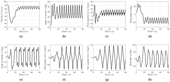
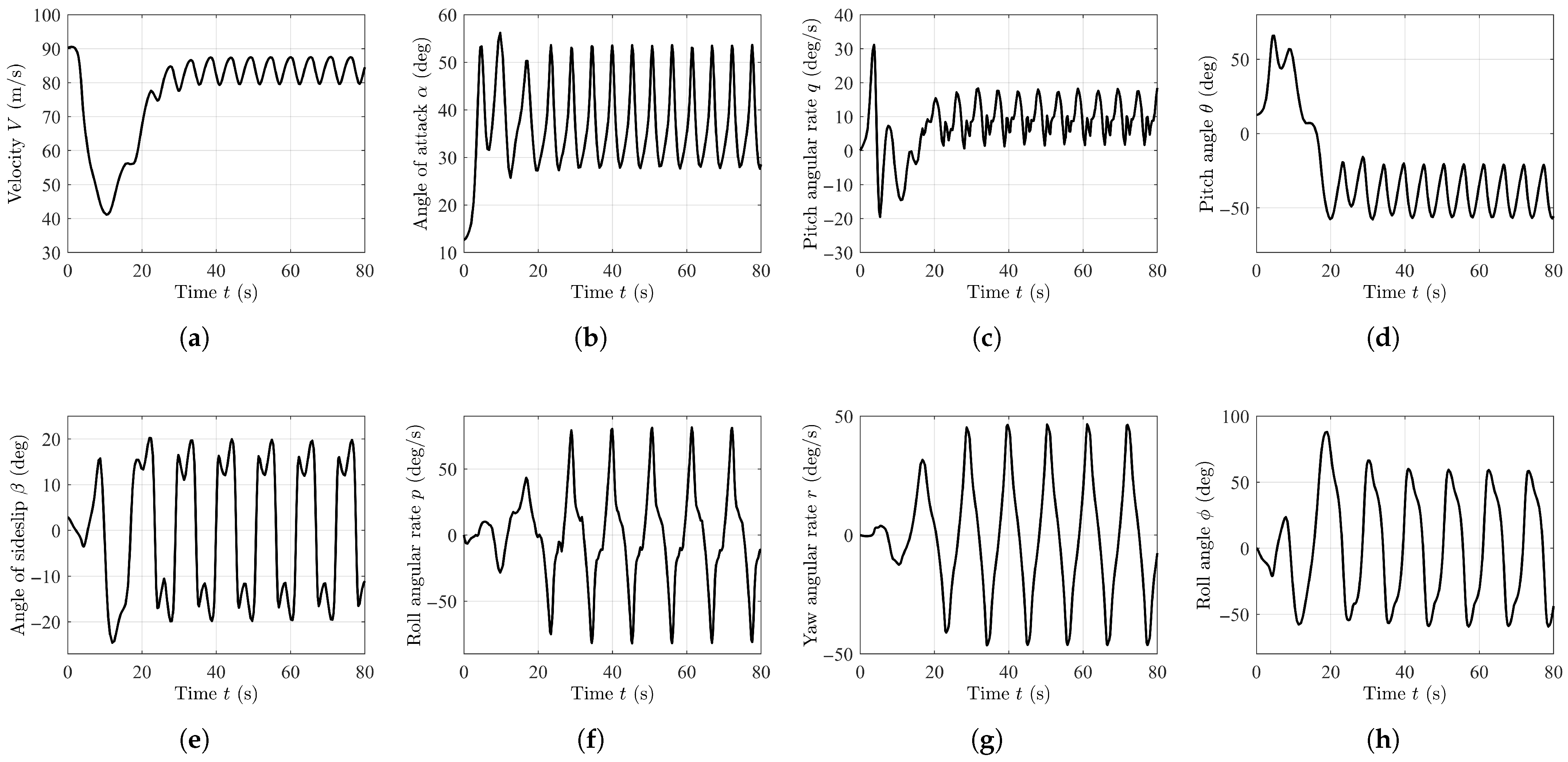
To illustrate the dynamic characteristics of wing rock, this study presents the open-loop evolution of the UAV from steady-level flight to the onset of wing rock. The initial flight state is set at an altitude of 5000 m and a velocity of 90.67 m/s, with a trimmed angle of attack of 12.54°. A sideslip disturbance of 2.8° is applied at the initial moment. Due to the longitudinal and directional instabilities inherent in the flying wing, the flight states naturally diverge under open-loop conditions. Figure 2 shows representative flight states, where Figure 2a–d illustrate longitudinal motion, and Figure 2e–h illustrate lateral-directional motion.

Figure 2. Time histories of longitudinal and lateral–directional flight state. (a–d) represent the longitudinal flight states, corresponding to velocity, angle of attack, pitch rate, and pitch angular angle, respectively. (e–h) represent the lateral–directional flight states, corresponding to sideslip angle, roll angular rate, yaw angular rate, and roll angle, respectively.

As shown in Figure 2b, the angle of attack rises sharply during the initial phase, quickly exceeding the stall angle of 38°. The pitch angle also increases markedly, resulting in a pronounced nose-up attitude, as shown in Figure 2d. The rapid rise in angle of attack significantly increases drag, causing airspeed to drop rapidly to about 42 m/s. After 10 s, the angle of attack gradually stabilizes into oscillation, while the pitch angle decreases sharply, indicating a nose-down attitude. At this stage, the UAV has entered a stall condition, and altitude decreases rapidly as gravitational potential energy converts into kinetic energy, leading to a gradual recovery of airspeed to around 85 m/s.

As shown in Figure 2e, the sideslip angle does not diverge directly but instead decreases initially, then increases, and ultimately settles into a limit cycle oscillation. This behavior stems from the coupling between lateral and directional motions, where the initial response exhibits a typical Dutch roll mode. As illustrated in Figure 2e,h, the flying wing is laterally stable: a positive sideslip disturbance induces a negative rolling motion. Under a negative roll attitude, the gravitational component along the $-y$ axis generates a negative sideslip, which then induces a positive rolling motion. Conversely, under a positive roll attitude, the gravitational component along the $+y$ axis produces a positive sideslip. When the angle of attack exceeds 40° and the sideslip angle surpasses 18°, both pitch and yaw stability are restored; however, the disturbance can no longer be suppressed, and the UAV eventually enters a limit cycle oscillation.

The limit cycle oscillation associated with wing rock exhibits several key characteristics:

(1) The angle of attack oscillates approximately around the stall angle;

(2) The pitch angle remains below zero, with longitudinal motion oscillating about a negative mean value;

(3) The roll angle, sideslip angle, roll rate, and yaw rate oscillate symmetrically around zero.

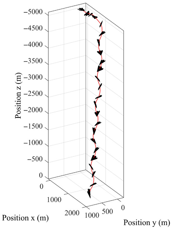
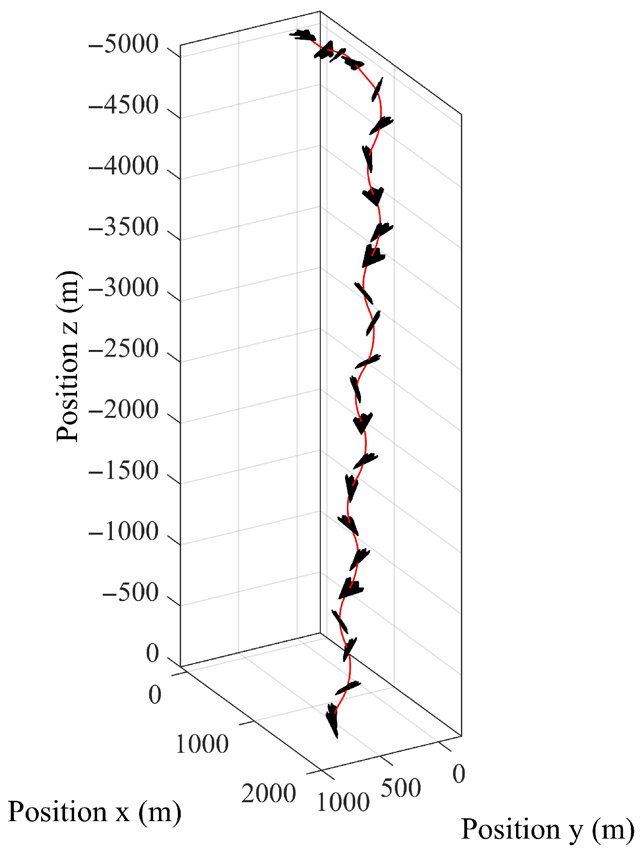
Figure 3 illustrates the three-dimensional trajectory and attitude of the UAV as it transitions from steady-level flight to the wing rock state. It can be observed that during the initial unstable phase, the UAV pitches up rapidly, while the loss of altitude remains relatively small. Subsequently, the UAV pitches down sharply and enters a near-vertical spiral descent. When viewed solely from the flight trajectory, this motion may appear similar to a spin mode. However, it is important to note that wing rock is distinct from spin motion. The fundamental difference lies in the center of oscillation of the lateral–directional states: in a spin motion, the lateral–directional oscillation centers are nonzero, as discussed in study [35]. From a physical perspective, the oscillation in wing rock originates from alternating stall phenomena between the left and right wings, whereas spin motion is sustained by continuous aerodynamic asymmetry in lift between the two wings induced by autorotation.

Figure 3. Flight trajectory of wing rock.

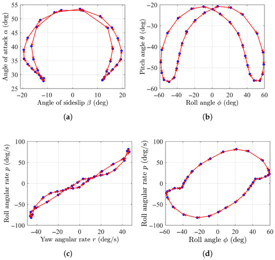
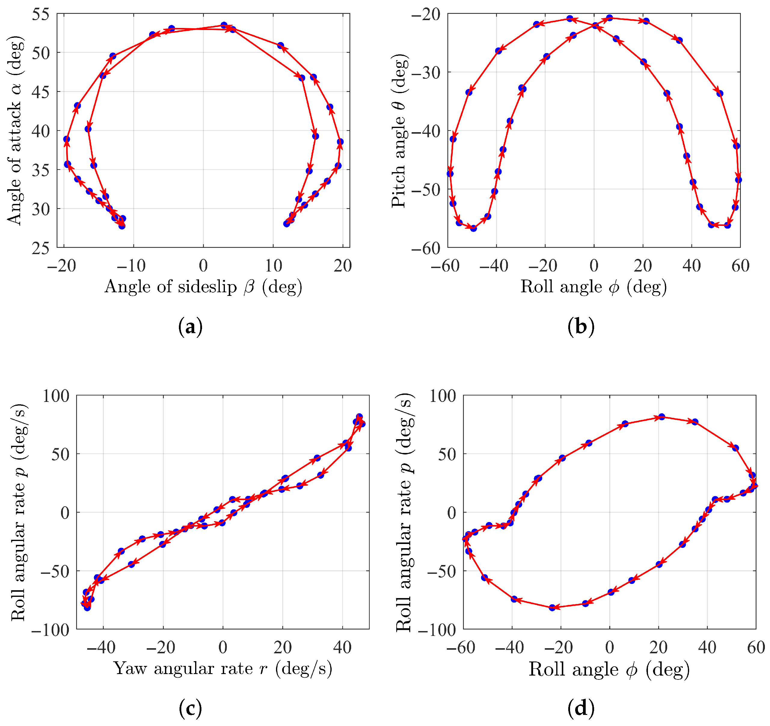
Figure 4 show the phase portraits of the wing rock motion, where the arrows indicate the direction of the motion trajectories. The phase portraits reveal that the wing rock motion is a stable limit cycle oscillation; regardless of the initial conditions, the system eventually converges to the same closed trajectory. In addition to illustrating the characteristics of the motion trajectory and amplitude, the shape of the limit cycle also reflects the degree of nonlinearity in the system. A circular or elliptical shape indicates weak nonlinearity, suggesting near-harmonic oscillation, whereas distorted or sharp-cornered shapes signify strong nonlinearity. As shown in Figure 4a–d, the phase portraits exhibit noticeable distortions and sharp corners, indicating that the wing rock exhibits strong nonlinear behavior. In particular, Figure 4c,d display twisted and pointed elliptical shapes, implying that the roll rate dynamics are highly nonlinear.

Figure 4. Phase portraits of wing rock motion. (a) represents the phase portrait of angle of attack and sideslip angle. (b) represents the phase portrait of roll angle and pitch angle. (c) represents the phase portrait of yaw angular rate and roll angular rate. (d) represents the phase portrait of roll angle and roll angular rate.

3. Control Law Design

This chapter presents the design process of the EINDI controller based on aerodynamic angular rate feedback. The same control framework can be applied to both wing rock recovery and maneuvering flight. Section 3.1 introduces the overall control architecture, while Section 3.2, Section 3.3 and Section 3.4 describe the inner loop for angular rate control, the outer loop for aerodynamic attitude control, and the velocity control law design, respectively.

3.1. Control Architecture

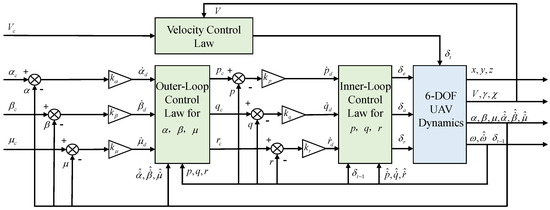
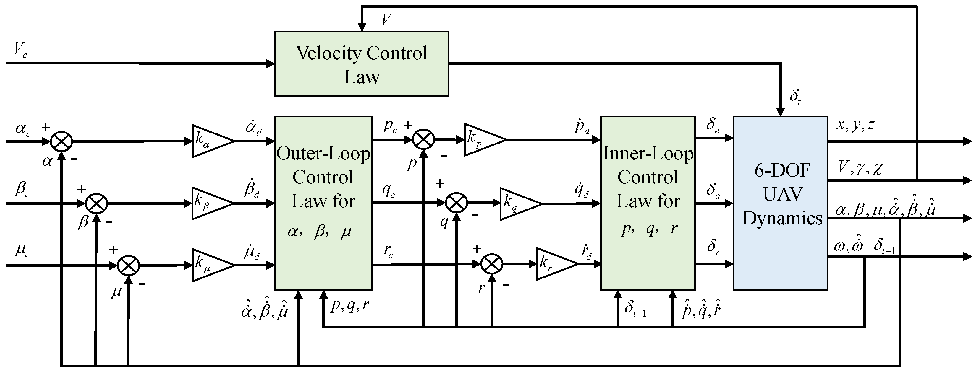
Figure 5 illustrates the control architecture proposed in this paper. The objective of flight control is to maintain the flight states at their desired values. A complete description of UAV motion requires 12 state variables, while the control input vector $\mathit{u}$ typically contains only four components, expressed as ${\left[{\delta }_e,{\delta }_T,{\delta }_a,{\delta }_r\right]}^T$. This discrepancy indicates that the UAV is a typical underactuated system. Cascaded control addresses this challenge by decomposing a complex control problem into multiple serially connected control loops. Its theoretical foundation lies in the principle of time-scale separation, which states that the flight states of the system can be divided into fast and slow dynamics, with the fast dynamics evolving significantly more rapidly than the slow ones. Based on this principle, the control system is structured into inner and outer loops: the output of the outer loop serves as the command for the inner loop. For UAV, angular rates ${\left[p,q,r\right]}^T$ represent the fast dynamics, whereas aerodynamic angles ${\left[\alpha ,\beta ,\mu \right]}^T$ represent the slow dynamics. Accordingly, this study adopts angular rate control as the inner loop and aerodynamic-angle control as the outer loop. UAV position and flight-path angles evolve even more slowly and their regulation depends on the stable control of both angular rates and aerodynamic angles. Position and flight-path control typically involve higher-level decision-making and trajectory planning, for which the control of angular rates and aerodynamic angles provides essential prerequisites. Velocity control is designed separately because velocity can be directly regulated through the throttle.

Figure 5. Control architecture of EINDI with aerodynamic angular rate feedback.

As shown in Figure 5, the block labeled “6-DOF UAV Dynamics” in the blue box represents the flight dynamics model that describes the complete 6-DOF motion of the UAV, that is, the system of differential equations given in Equations (1)–(12). The inputs to this module are the elevator, aileron, rudder, and throttle commands, and its outputs are the flight states. This module incorporates the aerodynamic model, gravity model, engine thrust model, and the associated coordinate-transformation matrices. In addition, this module records the estimated angular acceleration, the estimated aerodynamic angular rate, and the control inputs from the previous time step, all of which are required in the subsequent control law design.

On the far left of the control framework are the control command inputs, namely the airspeed command, angle-of-attack command, sideslip-angle command, and velocity-roll-angle command. The three aerodynamic-angle control commands are compared with the corresponding feedback states to obtain the state errors. These errors are multiplied by the aerodynamic-angle proportional gains to generate the first-order derivative commands of the aerodynamic angles, which are then sent to the outer-loop control-law design module. This module also takes the estimated aerodynamic angular rates and the body angular rates as inputs and outputs the angular rate control commands, denoted as ${\left[p_c,q_c,r_c\right]}^T$. The angular rate control commands are compared with the measured angular rates to obtain the angular rate errors, which are then multiplied by the angular rate proportional gains to produce the first-order derivative commands of the angular rates. These commands are passed into the inner-loop control-law design module. The inner-loop module also requires the estimated angular accelerations and the control surface deflection commands from the previous time step as inputs, and generates the updated control-surface deflection commands. For the velocity-control module, the airspeed command and the feedback airspeed serve as the inputs, and the module outputs the corresponding throttle command.

3.2. Inner Loop for Angular Rate Control

In this paper, the classical INDI approach is adopted for the design of the inner-loop control law. The stability of this method has been rigorously and comprehensively established by Xuerui Wang [36] and co-workers. The objective of the inner-loop controller is to achieve precise tracking of the UAV’s angular rates ${\left[p,q,r\right]}^T$. Its design is based on the angular-motion dynamics of the UAV, namely Equations (4)–(6). These three equations can be expressed in matrix form as follows:

$$\dot{\mathit{\omega }}={\mathit{f}}_{\mathbf{1}}\left(\mathit{x}\right)+{\mathit{G}}_{\mathbf{1}}\left(\mathit{x}\right)\mathit{u}$$

(29)

Here, $\mathit{\omega }$ denotes the body angular rate, ${\mathit{f}}_{\mathbf{1}}$ represents the terms in the equations that are independent of the control inputs, and ${\mathit{G}}_{\mathbf{1}}$ is the control effectiveness function of actuators. By applying a first-order Taylor expansion to Equation (29) over one time step $\Delta t$, Equation (30) is obtained:

$$\dot{\mathit{\omega }}={\dot{\mathit{\omega }}}_{\mathbf{0}}+{\left.{\displaystyle \frac{\mathit{\partial }\left[{\mathit{f}}_{\mathbf{1}}\left(\mathit{x}\right)+{\mathit{G}}_{\mathbf{1}}\left(\mathit{x}\right)\mathit{u}\right]}{\mathit{\partial }\mathit{x}}}\right|}_{\mathbf{0}}\Delta \mathit{x}+{\mathit{G}}_{\mathbf{2}}\left({\mathit{x}}_{\mathbf{0}}\right)\Delta \mathit{u}+{\mathit{R}}_{\mathbf{1}}$$

(30)

Here, $\Delta \mathit{x}$ denotes the increment of the state, $\Delta \mathit{u}$ denotes the increment of the control input, ${\mathit{\omega }}_{\mathbf{0}}$ and ${\mathit{x}}_{\mathbf{0}}$ denote the angular rate and flight state at the initial time step, and $\mathit{R}$ represents the higher-order remainder of the expansion. The core assumption employed by INDI is that the control-input variation is much faster than the variation of the flight states. In other words, over the interval $\Delta t$, the change of the flight state is negligible compared with the change of the control input, which means $\Delta \mathit{u}\gg \Delta \mathit{x}$. Based on this assumption, the related state-dependent terms and the higher-order remainder $\mathit{R}$ can be neglected. Consequently, Equation (31) is obtained.

$$\dot{\mathit{\omega }}\approx {\dot{\mathit{\omega }}}_{\mathbf{0}}+{\mathit{G}}_{\mathbf{1}}\left({\mathit{x}}_{\mathbf{0}}\right)\Delta \mathit{u}$$

(31)

Here, the control effectiveness matrix ${\mathit{G}}_{\mathbf{1}}$ can be determined from the control derivatives of the control surfaces, the dynamic pressure, and the basic parameters of the UAV. In essence, ${\mathit{G}}_{\mathbf{1}}$ represents the Jacobian matrix of the moment equations with respect to the control surface deflections, that is, Equation (32):

$${\mathit{G}}_{\mathbf{1}}\left({\mathit{x}}_{\mathbf{0}}\right)=\left[\begin{array}{ccc}{\displaystyle \frac{\partial \dot{p}}{\partial {\delta }_e}}& {\displaystyle \frac{\partial \dot{p}}{\partial {\delta }_a}}& {\displaystyle \frac{\partial \dot{p}}{\partial {\delta }_r}}\\ {\displaystyle \frac{\partial \dot{q}}{\partial {\delta }_e}}& {\displaystyle \frac{\partial \dot{q}}{\partial {\delta }_a}}& {\displaystyle \frac{\partial \dot{q}}{\partial {\delta }_r}}\\ {\displaystyle \frac{\partial \dot{r}}{\partial {\delta }_e}}& {\displaystyle \frac{\partial \dot{r}}{\partial {\delta }_a}}& {\displaystyle \frac{\partial \dot{r}}{\partial {\delta }_r}}\end{array}\right]$$

(32)

If the commanded angular rate and the current angular rate are known, the desired angular acceleration can be obtained from Equations (33)–(35):

$${\dot{p}}_d=K_p\left(p_c-p\right)$$

(33)

$${\dot{q}}_d=K_q\left(q_c-q\right)$$

(34)

$${\dot{r}}_d=K_r\left(r_c-r\right)$$

(35)

Let the estimated angular acceleration feedback from the UAV at each moment be ${\left[\widehat{\dot{p}},\widehat{\dot{q}},\widehat{\dot{r}}\right]}^T$. By taking the inverse of Equation (31), the required control input increment to achieve the control objective can be obtained. It can be expressed in component form as follows:

$$\left[\begin{array}{c}\Delta {\delta }_e\\ \Delta {\delta }_a\\ \Delta {\delta }_r\end{array}\right]={\mathit{G}}_{\mathbf{1}}^{-\mathbf{1}}\left({\mathit{x}}_{\mathbf{0}}\right)\left(\left[\begin{array}{c}{\dot{p}}_d\\ {\dot{q}}_d\\ {\dot{r}}_d\end{array}\right]-\left[\begin{array}{c}\widehat{\dot{p}}\\ \widehat{\dot{q}}\\ \widehat{\dot{r}}\end{array}\right]\right)$$

(36)

At this moment, the control command for the control surface deflection should be the sum of the current control surface deflection and the computed control input increment. Therefore, the control surface deflection command can be expressed as

$$\left[\begin{array}{c}{\delta }_e\\ {\delta }_a\\ {\delta }_r\end{array}\right]=\left[\begin{array}{c}\Delta {\delta }_e\\ \Delta {\delta }_a\\ \Delta {\delta }_r\end{array}\right]+\left[\begin{array}{c}{\delta }_{e_0}\\ {\delta }_{a_0}\\ {\delta }_{r_0}\end{array}\right]$$

(37)

3.3. Outer Loop for Aerodynamic Attitude Control

3.3.1. Enhanced INDI (EINDI)

In this paper, the outer-loop control law that incorporates aerodynamic angular rate feedback is referred to as enhanced INDI (EINDI), in order to clearly distinguish it from other outer-loop control strategies.

The design of the outer-loop control law is based on the dynamics of the aerodynamic angles, namely Equations (23)–(25). These equations can be expressed in matrix form as Equation (38). In this formulation, the terms associated with the body angular rates are grouped together, while the terms associated with external forces are denoted by $f_{\alpha }, f_{\beta }$ and $f_{\mu }$.

$$\left[\begin{array}{c}\dot{\alpha }\\ \dot{\beta }\\ \dot{\mu }\end{array}\right]=\left[\begin{array}{c}{f}_{\alpha }\\ f_{\beta }\\ f_{\mu }\end{array}\right]+{\mathit{G}}_{\mathbf{2}}\left[\begin{array}{c}p\\ q\\ r\end{array}\right]$$

(38)

In this formulation, the $f_{\alpha },f_{\beta }$, $f_{\mu }$ and the matrix ${\mathit{G}}_{\mathbf{2}}$ are defined by Equations (39)–(42), respectively.

$$f_{\alpha }={\displaystyle \frac{1}{mV\cos \beta }}\left(-L-T\sin \alpha +mg\cos \gamma \cos \mu \right)$$

(39)

$$f_{\beta }={\displaystyle \frac{1}{mV}}\left(-T\cos \alpha \sin \beta +Y\cos \beta +mg\cos \gamma \sin \mu \right)$$

(40)

$$\begin{array}{c}{f}_{\mu }=-{\displaystyle \frac{g}{V}}\cos \gamma \cos \mu \tan \beta \hfill \\ +{\displaystyle \frac{1}{mV}}\left[L\left(\tan \gamma \sin \mu +\tan \beta \right)+Y\tan \gamma \cos \mu \cos \beta \right]\hfill \end{array}$$

(41)

$${\mathit{G}}_{\mathbf{2}}=\left[\begin{array}{ccc}-\tan \beta \cos \alpha & 1& -\tan \beta \sin \alpha \\ \sin \alpha & 0& -\cos \alpha \\ \sec \beta \cos \alpha & 0& \sec \beta \sin \alpha \end{array}\right]$$

(42)

The objective of the inner-loop control law is to regulate the aerodynamic angles to their desired target values. This is achieved by generating the corresponding angular rate commands based on the current aerodynamic angles. Let the commanded aerodynamic angles be denoted as ${\alpha }_c$, ${\beta }_c$ and ${\mu }_c$; then, the desired first derivatives of the aerodynamic angles can be obtained from the following equation:

$${\dot{\alpha }}_d=K_{\alpha }\left({\alpha }_c-\alpha \right)$$

(43)

$${\dot{\beta }}_d=K_{\beta }\left({\beta }_c-\beta \right)$$

(44)

$${\dot{\mu }}_d=K_{\mu }\left({\mu }_c-\mu \right)$$

(45)

The matrix ${\mathit{G}}_{\mathbf{2}}$ can be directly computed in real time using the measured angle of attack and sideslip angle obtained from the onboard sensors. If the complete UAV system model is known, that is, the explicit expressions of $f_{\alpha }, f_{\beta }$ and $f_{\mu }$ are available, the angular rate command can in principle be obtained by directly inverting Equation (38). However, obtaining an accurate system model is generally challenging, primarily for two reasons. First, the aerodynamic forces at high angles of attack are highly nonlinear and unsteady. Under the constraints of limited CFD data and wind tunnel measurements, accurate aerodynamic modeling itself poses a significant challenge. For low-aspect-ratio flying wings, the nonlinear and unsteady aerodynamic effects caused by the breakdown of leading-edge vortices during high-angle-of-attack maneuvers are even more pronounced. Second, aerodynamic forces are subject to strong uncertainties. Factors such as wind tunnel measurement errors, external disturbances in actual flight conditions, and sensor inaccuracies introduce considerable uncertainty in aerodynamic calculations. Previous studies have shown that nonlinear dynamic inversion (NDI) control is highly sensitive to modeling errors; thus, using onboard models during high-dynamic maneuvers entails significant risk, necessitating the development of control methods with lower model dependence and higher robustness.

INDI reduces reliance on the system model by employing angular acceleration feedback. Fundamentally, angular acceleration is generated by the total external moments acting on the UAV, thereby encapsulating information about the UAV’s rotational motion. Regardless of model inaccuracies or external disturbances, angular acceleration inherently contains the true information of the applied external moments. To date, the use of INDI has been largely limited to angular acceleration feedback and is therefore commonly applied in inner-loop control-law design. Inspired by the sensor-based dynamic inversion concept, this study innovatively employs aerodynamic angular rate as the feedback variable, enabling the design of an outer-loop control law under a model-free condition.

Assuming that the estimated aerodynamic angular rate ${\left[\widehat{\dot{\alpha }},\widehat{\dot{\beta }},\widehat{\dot{\mu }}\right]}^T$ is available as a feedback signal, the corresponding system model functions $f_{\alpha }, f_{\beta }$ and $f_{\mu }$ in Equation (38) can be directly estimated as follows:

$$\left[\begin{array}{c}{\widehat{f}}_{\alpha }\\ {\widehat{f}}_{\beta }\\ {\widehat{f}}_{\mu }\end{array}\right]=\left[\begin{array}{c}\widehat{\dot{\alpha }}\\ \widehat{\dot{\beta }}\\ \widehat{\dot{\mu }}\end{array}\right]-{\mathit{G}}_{\mathbf{2}}\left[\begin{array}{c}p\\ q\\ r\end{array}\right]$$

(46)

Here, ${\mathit{G}}_{\mathbf{2}}$ and the UAV body angular rates are known quantities. Therefore, Equation (38) is fully solvable. Based on Equations (43)–(45) and Equation (46), the angular rate command required to achieve the aerodynamic-angle control objective can be computed directly as

$$\left[\begin{array}{c}{p}_c\\ q_c\\ r_c\end{array}\right]={\mathit{G}}_{\mathbf{2}}^{-\mathbf{1}}\left(\left[\begin{array}{c}{\dot{\alpha }}_d\\ {\dot{\beta }}_d\\ {\dot{\mu }}_d\end{array}\right]-\left[\begin{array}{c}{\widehat{f}}_{\alpha }\\ {\widehat{f}}_{\beta }\\ {\widehat{f}}_{\mu }\end{array}\right]\right)$$

(47)

As with the angular acceleration used in the inner loop, the aerodynamic angular rates ${[\widehat{\dot{\alpha }},\widehat{\dot{\beta }},\widehat{\dot{\mu }}]}^T$ cannot be measured directly. Their acquisition in practice involves two steps: estimating the aerodynamic angles themselves and then estimating their time derivatives.

For the aerodynamic angles, the angle of attack $\alpha$ and sideslip angle $\beta$ can be measured by air-data sensors. On large aircraft, dedicated air-data systems with mechanical vanes are routinely employed; for smaller UAVs, multi-hole pressure probes (e.g., five-hole probes) and miniaturized vane-based sensors using Hall-effect transducers are commercially available. The velocity roll angle $\mu$ is not measured directly but is obtained from the kinematic relation in Equation (16), which combines the body-axis attitude (provided by the onboard IMU and an attitude estimator) with the measured $\alpha$ and $\beta$. The derivatives $\widehat{\dot{\alpha }},\widehat{\dot{\beta }},\widehat{\dot{\mu }}$ are then estimated by fusing the sensor measurements with inertial information through filtering and state-estimation techniques such as the extended Kalman filter or the complementary filter, in the same manner that the angular acceleration $\widehat{\dot{\omega }}$ used by classical INDI is obtained from gyro measurements.

Sensor-based estimation of $\alpha$, $\beta$ and their derivatives in the presence of measurement noise, sensor lag, and rapidly varying flight states is an active engineering topic, and the development of high-bandwidth, high-accuracy estimators for these quantities is part of our ongoing work. The present paper focuses on the controller design and its theoretical validation, while the corresponding sensor integration and estimator performance will be reported separately.

Equation (46) is a fundamental relation in this work because it implies that once the aerodynamic angular rate is available, the system model functions can be computed directly. These model functions are related to the net external moments and forces acting on the UAV, and here we effectively replace an explicit model of those net moments with information derived from sensors.

3.3.2. Linear Outer Loop (P-INDI and PI-INDI)

In [30], a decoupled INDI control law was proposed, in which the outer loop directly generates angular rate commands through proportional control of the attitude angle errors, as shown in Equations (48)–(50). In this paper, this proportional linear outer-loop control strategy is denoted as P-INDI.

$$p_c=K_{\mu }\left({\mu }_c-\mu \right)$$

(48)

$$q_c=K_{\alpha }\left({\alpha }_c-\alpha \right)$$

(49)

$$r_c=K_{\beta }\left({\beta }_c-\beta \right)$$

(50)

Simulation results indicate that the proportional linear outer loop may lead to relatively large steady-state errors. Therefore, a proportional–integral outer-loop control law is additionally introduced for comparative purposes and is referred to as PI-INDI. The governing equations of the PI outer-loop control law are given in Equations (51)–(53).

$$p_c=K_{\mu }\left({\mu }_c-\mu \right)+K_{\mu }^I\int \left({\mu }_c-\mu \right)dt$$

(51)

$$q_c=K_{\alpha }\left({\alpha }_c-\alpha \right)+K_{\alpha }^I\int \left({\alpha }_c-\alpha \right)dt$$

(52)

$$r_c=K_{\beta }\left({\beta }_c-\beta \right)+K_{\beta }^I\int \left({\beta }_c-\beta \right)dt$$

(53)

3.3.3. Nonlinear Outer Loop (NDI-INDI and SNDI-INDI)

As a benchmark configuration, the combination of a nonlinear dynamic inversion (NDI) [37] outer-loop controller designed using accurate onboard model information and an INDI inner-loop controller is denoted as NDI-INDI in this paper.

In [31], the authors computed angular rate commands based on flight-path state information $\dot{\gamma }$ and $\dot{\chi }$. However, in scenarios where navigation information is unreliable, the flight-path state information may not be available. To assess this scenario, the present study directly removes the terms related to flight-path states and retains only the aerodynamic-angle-related terms, as shown in Equation (54). Further analysis reveals that the matrix appearing in Equation (54) is, in fact, an equivalent transformation of the inverse of matrix ${\mathit{G}}_{\mathbf{2}}$. In other words, if the system state functions $f_{\alpha }, f_{\beta }$ and $f_{\mu }$ are neglected and only motion-related terms are preserved, angular rate commands can still be approximately computed. Consequently, neglecting flight-path state information is equivalent to neglecting the system state function. The combination of this simplified outer-loop control law with the INDI inner-loop controller is referred to as SNDI-INDI in this paper.

$$\left[\begin{array}{c}{p}_c\\ q_c\\ r_c\end{array}\right]=\left[\begin{array}{ccc}0& \sin \alpha & \cos \alpha \cos \beta \\ 1& 0& \sin \beta \\ 0& -\cos \alpha & \sin \alpha \cos \beta \end{array}\right]\left[\begin{array}{c}{\dot{\alpha }}_d\\ {\dot{\beta }}_d\\ {\dot{\mu }}_d\end{array}\right]$$

(54)

3.4. Velocity Control

Since the engine thrust has a direct influence on the UAV’s velocity, the throttle command can be used to control the airspeed directly. A simple proportional control strategy is adopted for the velocity control. Based on the velocity command and the current velocity V, the throttle setting can be determined by Equation (55):

$${\delta }_t=K_V\left(V_c-V\right)$$

(55)

where Kt is the throttle proportional gain.

3.5. Controller Gain Selection

The proposed control framework involves the inner-loop angular rate gains $K_p$, $K_q$, $K_r$, and the outer-loop aerodynamic-angle gains $K_{\alpha }$, $K_{\beta }$, $K_{\mu }$. For the PI-INDI variant, additional integral gains $K_{\alpha }^I$, $K_{\beta }^I$, $K_{\mu }^I$ are introduced. The specific values used in all simulations are summarized in Table 3.

Table 3. Controller gains used in the simulations.

Method	Loop/Gain	Value (rad/s)	Notes
All methods	$K_p$	13	Inner loop (INDI)
	$K_q$	12
	$K_r$	8
	$K_V$	1.6	Velocity loop
EINDI, NDI-INDI, SNDI-INDI	$K_{\alpha }$	1.6	Outer loop (P), nonlinear
	$K_{\beta }$	1.3
	$K_{\mu }$	1.0
P-INDI, PI-INDI	$K_{\alpha }$	0.5	Outer loop (P), linear
	$K_{\beta }$	−0.1
	$K_{\mu }$	1.0
PI-INDI only	$K_{\alpha }^I$	0.2	Outer loop (I)
	$K_{\beta }^I$	−0.01
	$K_{\mu }^I$	0.05

Following the cascaded design strategy of [31], each proportional gain corresponds to the bandwidth of its associated loop, and a sufficient separation between inner- and outer-loop bandwidths is required to preserve time-scale separation. In this work, the inner-loop gains are placed in the range of 8–13 $\mathrm{rad}/\mathrm{s}$, and the outer-loop gains in the range of $1.0$–$1.6\mathrm{rad}/\mathrm{s}$, yielding a separation ratio of approximately 8 to 10.

For the linear outer-loop methods (P-INDI, PI-INDI), the proportional gains differ from those of the nonlinear methods, and the sign of $K_{\beta }$ differs as well, reflecting the different control law structures. All gains were obtained through tuning and represent the best results achieved for each method.

4. Results

This chapter presents the results of applying EINDI to wing rock recovery control, together with a comparative evaluation of different control strategies under model uncertainty. Section 4.1 examines whether EINDI is capable of achieving effective recovery from wing rock motion. To demonstrate the effectiveness of EINDI as comprehensively as possible, 17 initial conditions distributed along the wing rock trajectory are selected as test cases. Section 4.2 provides a comparative assessment of the control performance of EINDI against other control approaches. Section 4.3 focuses on the differences in attitude command tracking performance among the considered control methods in the presence of model uncertainties, thereby highlighting their respective robustness characteristics.

4.1. Simulation of Different Initial Condition

As a typical limit cycle oscillation, the wing rock mode does not possess fixed flight states; instead, all states evolve continuously along a periodic trajectory. Because recovery control may be initiated at any point on this trajectory, assessing the effectiveness of EINDI for wing rock suppression requires evaluating the controller at multiple states along the cycle.

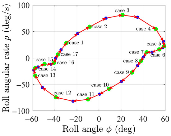
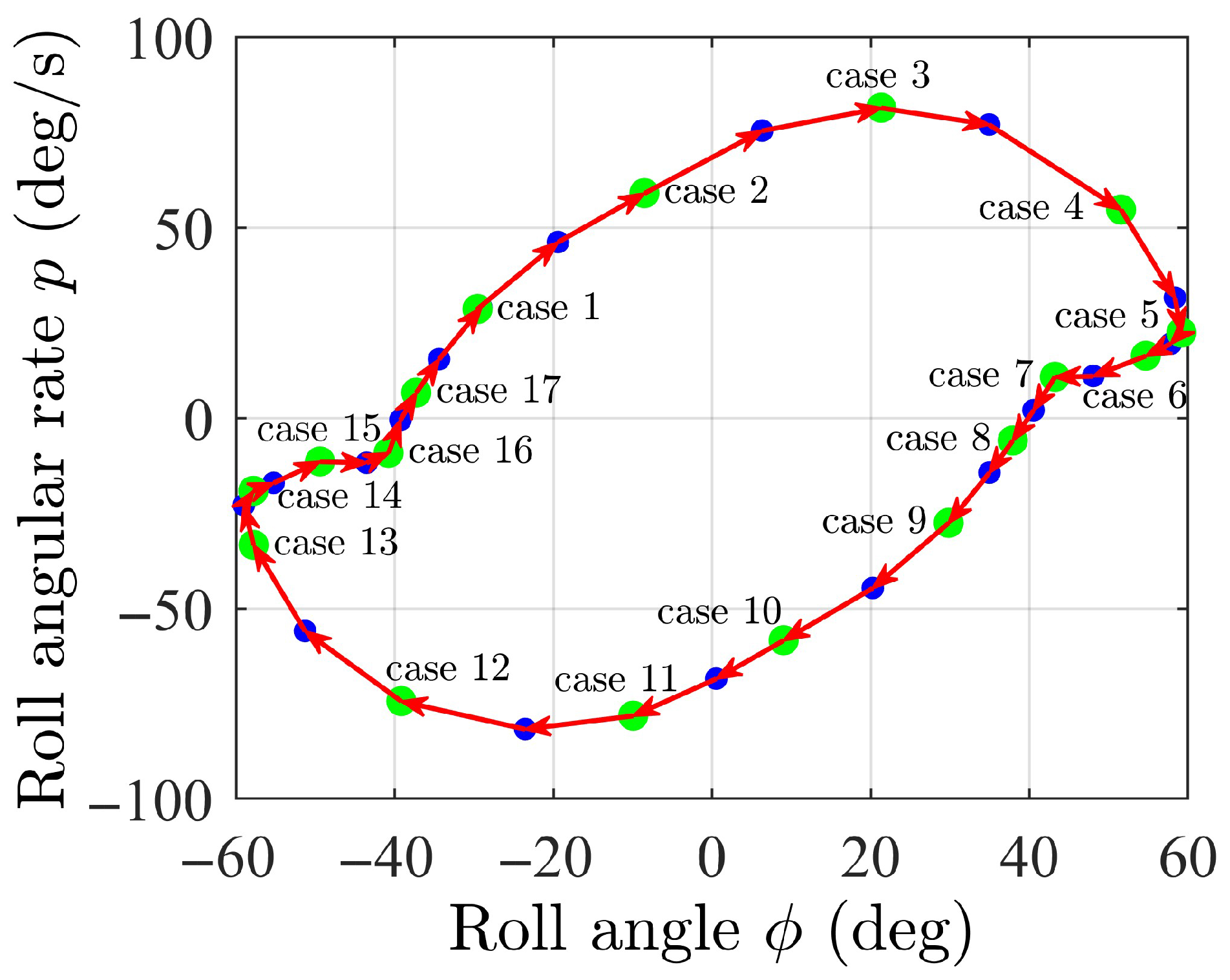
Given that wing rock motion is dominated by rolling dynamics, 17 representative points on the $\varphi$–p phase portrait were selected as initial conditions. These points, highlighted in green in Figure 6, span roll angles with an amplitude of approximately 60° and roll rates with an amplitude of approximately 80°/s.

Figure 6. Selected cases on the phase portrait of $\varphi , p$.

The simulation was initialized at an altitude of 5000 m, with the EINDI controller activated at the start of the run. The desired recovery state was straight-level flight at a speed of 100 m/s, corresponding to a trim angle of attack of 10.67°. Accordingly, the velocity command was set to 100 m/s, the angle-of-attack command to 10.67°, and both the velocity roll-angle and sideslip-angle commands were set to zero.

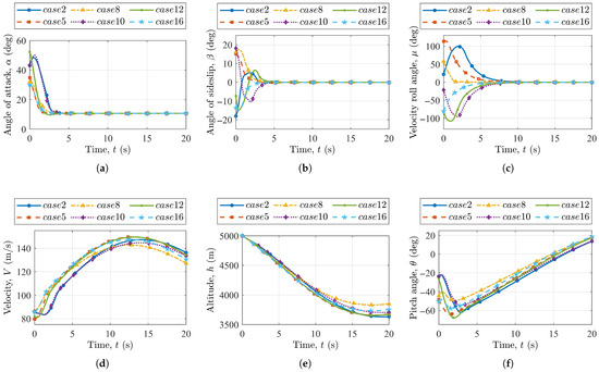
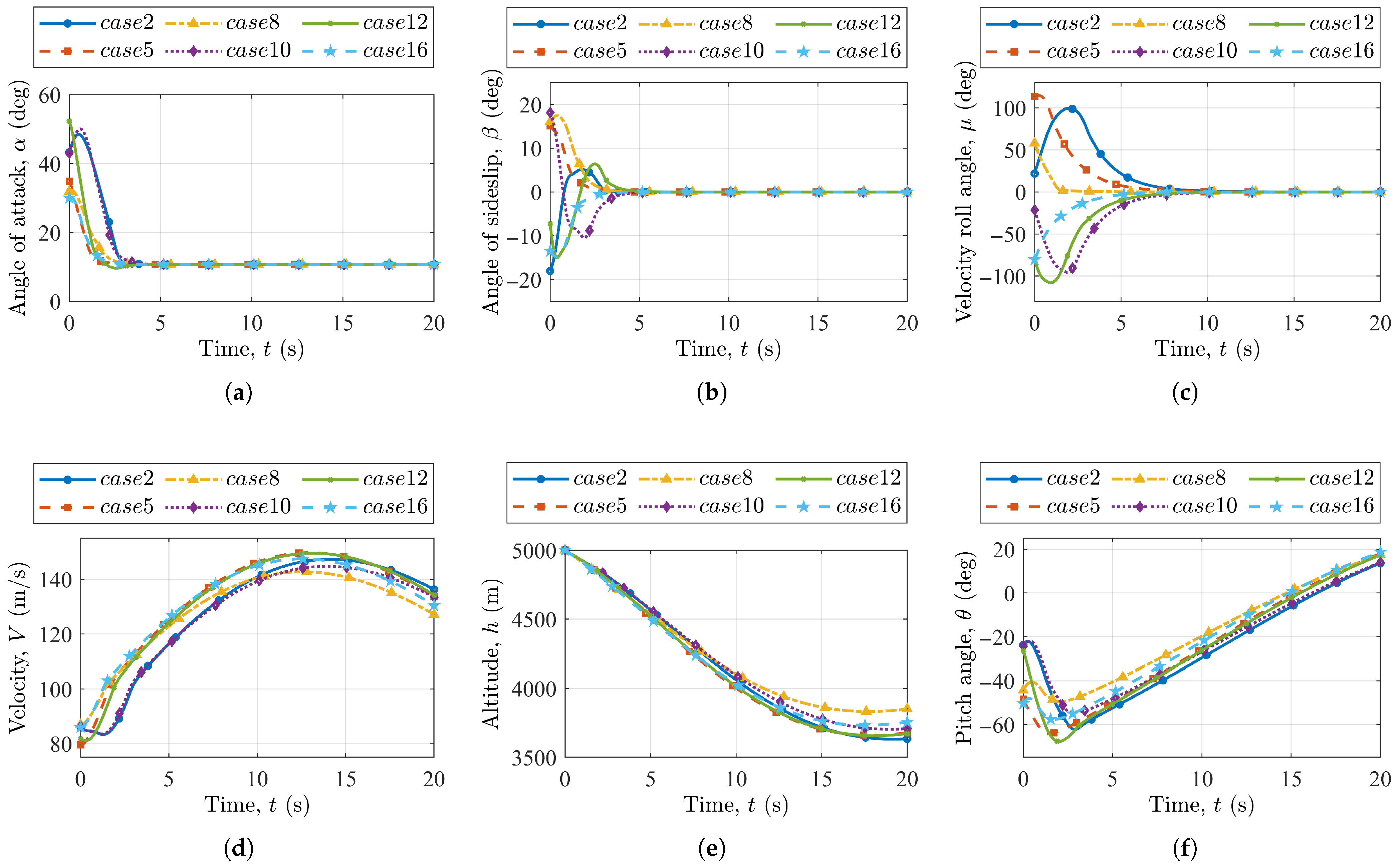
Figure 7 illustrates the wing rock recovery process for six representative initial states. As shown in Figure 7a, the initial angle of attack ranges from 30° to 52°. Although the convergence rates differ among the cases, all trajectories reach the commanded value at approximately 4 s. In Case 2 and Case 10, the angle of attack initially increases before decreasing, indicating that the angle-of-attack rates for these two states are positive at the start. Figure 7b shows the convergence of the sideslip angle, which proceeds slightly more slowly than the angle of attack and fully converges at around 5 s. The convergence of the velocity roll angle is presented in Figure 7c; this variable requires more time to settle than both the angle of attack and the sideslip angle, taking approximately 10 s. Figure 7d shows the speed response: before 13 s, the velocity gradually increases, whereas after 13 s it begins to decrease.

Figure 7. Six cases of wing rock recovery control using EINDI. (a–f) depict the time-domain evolution curves of angle of attack, sideslip angle, velocity roll angle, velocity, altitude, and pitch angle in the six cases, respectively.

During the initial phase of recovery control, the angle of attack, sideslip angle, and velocity roll angle decrease rapidly, enabling the UAV to exit the stalled condition and thereby reducing drag. At this stage, the pitch angle has not yet recovered, and the UAV maintains a diving attitude, which causes the airspeed to increase. After 13 s, lift is gradually restored, the descent rate decreases, and the pitch angle returns toward its commanded state. Because the airspeed remains above the target value, the throttle command is subsequently reduced, placing the UAV in a low-power condition and leading to a decrease in speed.

In the simulation tests, the UAV speed converges to the target value at approximately 40 s. This complete convergence is not fully reflected in Figure 7d because the UAV has already completed the wing rock recovery maneuver by 20 s. In this study, the completion of the recovery maneuver is defined as the moment when the altitude rate returns to zero, which occurs at approximately 18 s in Figure 7e. This definition is motivated by the fact that the primary hazard of the wing rock mode is not the oscillatory motion itself, but the onset of a near-vertical spiral descent that leads to substantial altitude loss. Once the fuselage is stabilized and altitude begins to recover, the UAV is considered to have exited the hazardous condition.

As shown in Figure 7e, from the onset of wing rock to the completion of recovery, the UAV experiences an altitude loss of approximately 1600 m. This indicates that, for the small-aspect-ratio flying wing considered in this study, the minimum safe recovery altitude for wing rock is at least 1600 m. In Figure 7f, the pitch angle remains oscillatory during the first 3.5 s. After the angle of attack recovers, the pitch angle gradually increases, and the UAV eventually exits the stalled, nose-down attitude.

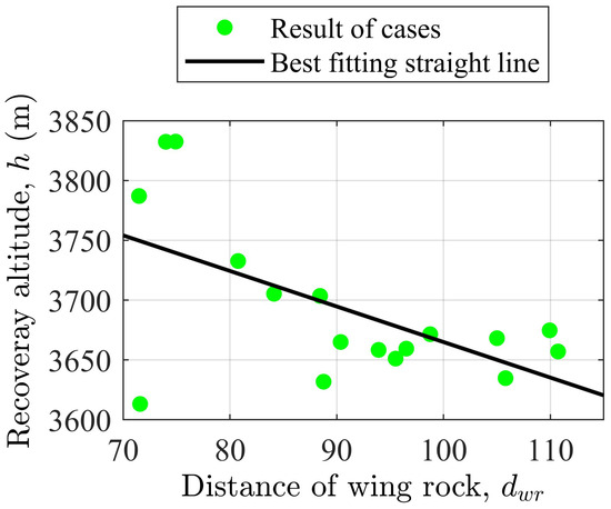
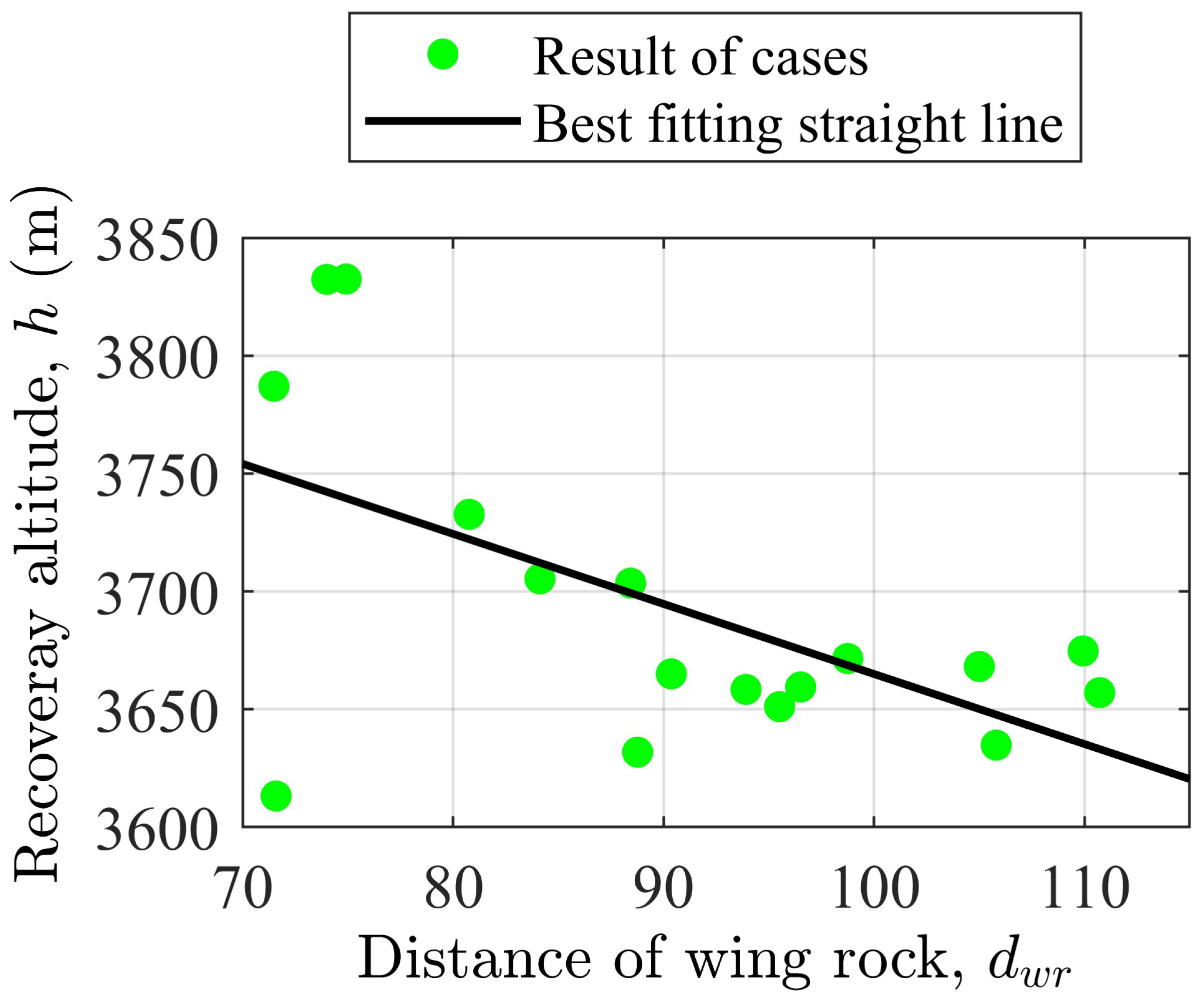
The simulation results demonstrate that the UAV successfully completes wing rock recovery from all tested initial states; however, the recovery altitude varies depending on the initial condition. Here, the recovery altitude is defined as the flight altitude at the moment the recovery maneuver is completed. This naturally raises the question of whether an optimal initial state exists along the wing rock trajectory that minimizes altitude loss during recovery. This study hypothesizes that the recovery altitude is negatively correlated with the Euclidean distance between the initial wing rock state and the target flight state. This distance, referred to as the distance of the initial wing rock state and defined in Equation (56), quantifies the separation between the two states. A smaller distance corresponds to a higher recovery altitude, whereas a larger distance leads to a lower recovery altitude.

$$d_{wr}=\sqrt{\begin{array}{c}{\left(V_0-V_d\right)}^2+{\left({\alpha }_0-{\alpha }_d\right)}^2+q_0^2+{\left({\theta }_0-{\theta }_d\right)}^2+{\beta }_0^2+p_0^2+r_0^2+{\varphi }_0^2\end{array}}$$

(56)

Under straight-level flight conditions, the trim values of ${\alpha }_d$ and ${\theta }_d$ are identical and expressed in degrees. The eight selected states were chosen because they represent critical flight conditions that strongly influence the UAV’s dynamic stability; in contrast, position and heading angles do not affect motion stability. To validate the hypothesis proposed in this study, the recovery altitudes and the corresponding Euclidean distances for all cases are summarized in Table 4.

Table 4. Result of all cases.

Cases	Recovery Altitude, h (m)	Distance of Initial Wing Rock State, ${\mathit{d}}_{\mathit{wr}}$
1	3787.014	71.4899388
2	3631.828	88.7705407
3	3674.75	109.935232
4	3668.2	105.003228
5	3659.46	96.5151082
6	3658.413	93.9211461
7	3705.307	84.1304022
8	3832.466	74.9217714
9	3613.237	71.5932893
10	3703.539	88.4395879
11	3634.795	105.806776
12	3657.074	110.722089
13	3671.528	98.7503714
14	3651.124	95.5152354
15	3665.016	90.3692374
16	3732.691	80.7678953
17	3832.327	74.0019779

Figure 8 presents the scatter distribution of the Euclidean distance versus the recovery altitude, with the black line representing the least-squares fit to the data. As shown in the figure, most points support the hypothesis that a larger distance corresponds to a lower recovery altitude. However, several points, such as Case 9, deviate noticeably from the fitted line, exhibiting both a small distance and a low recovery altitude. This deviation arises because, in highly nonlinear motions such as wing rock, the differences among initial states cannot be fully characterized by Euclidean distance alone; the initial direction of motion also plays an important role.

Figure 8. The correlation between the Euclidean distance of the initial state from the target state and the recovery altitude.

Overall, the Euclidean distance of the initial state remains the dominant factor. Therefore, when selecting an optimal initial state, one should choose the state closest to the target state. From a flight-safety perspective, once the UAV enters the wing rock mode, recovery control should be initiated as early as possible.

4.2. Comparison of Different Control Methods in Wing Rock Recovery

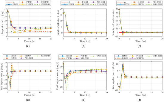
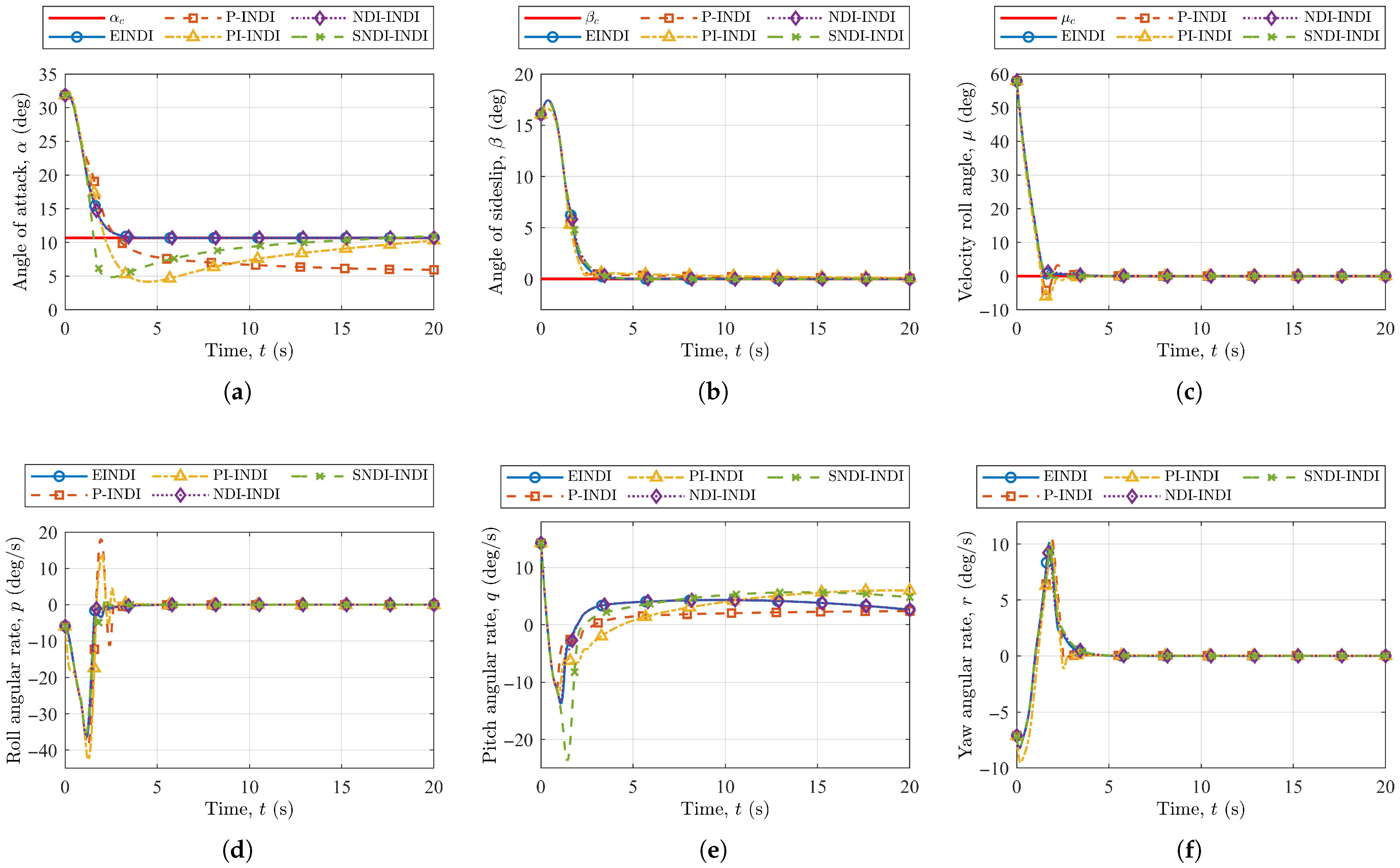
The simulation uses Case 8 as the initial state, and the results of the five control strategies are presented in Figure 9. As shown in Figure 9a, all methods achieve convergence of the angle of attack. P-INDI reaches the target angle in approximately 2.7 s but cannot maintain it, exhibiting a steady-state error of about 5°. In contrast, PI-INDI significantly reduces the steady-state error due to the integral term, but it exhibits larger overshoot than P-INDI and requires more time to eliminate the steady-state error. The SNDI-INDI scheme exhibits a faster response; however, it also shows pronounced overshoot. Compared with linear control strategies, EINDI and NDI-INDI demonstrate superior performance, with minimal overshoot and negligible steady-state error. The performance of EINDI is very close to that of NDI-INDI, indicating that aerodynamic angular rate feedback can achieve control results comparable to those of NDI with a known model.

Figure 9. Case 8 simulation results using EINDI, P-INDI, PI-INDI, NDI-INDI and SNDI-INDI. (a–f) depict the time-domain evolution curves of angle of attack, sideslip angle, velocity roll angle, roll angular rate, pitch angular rate, and yaw angular rate, respectively.

Figure 9b presents the sideslip angle response. The differences among the four control strategies are minor; linear methods respond slightly faster but exhibit small control errors near the target, which take longer to converge. EINDI and NDI-INDI, by contrast, show smoother responses with negligible steady-state error. Figure 9c depicts the velocity roll angle response, where linear control strategies exhibit significant overshoot, whereas EINDI and NDI-INDI maintain favorable control performance.

Figure 9d–f show the time responses of roll rate, pitch rate, and yaw rate. EINDI closely tracks NDI-INDI, whereas linear control strategies display substantial overshoot and oscillations. As shown in Figure 9e, SNDI-INDI exhibits a more pronounced overshoot. Since all methods employ standard INDI in the inner loop, these angular rate responses primarily reflect the outer-loop-generated angular rate control commands, demonstrating that EINDI produces more reasonable and smoother control signals.

To more quantitatively evaluate the differences in control performance among the considered control strategies, the integrated absolute error (IAE, ${\int }_0^t\left|e\left(t\right)\right|dt$) and integrated time absolute error (ITAE, ${\int }_0^{t}t\ast \left|e\left(t\right)\right|dt$) of the control variables are employed as performance metrics. As summarized in Table 5, for angle-of-attack command tracking, EINDI and NDI-INDI achieve the best performance, whereas P-INDI performs the worst. For sideslip-angle and velocity-roll-angle command tracking, the performance differences among the various methods are relatively minor.

Table 5. IAE and ITAE results for wing rock recovery control using different control strategies.

Control Method and Index	$\mathit{\alpha }$	$\mathit{\beta }$	$\mathit{\mu }$	p	q	r
EINDI (IAE)	25.9	25.6	39.3	34.6	79.2	14.2
P-INDI (IAE)	95.5	28.0	38.8	49.0	43.7	15.9
PI-INDI (IAE)	81.4	28.8	39.5	48.2	86.2	15.4
NDI-INDI (IAE)	25.8	26.4	39.9	34.4	79.3	14.2
SNDI-INDI (IAE)	54.7	26.4	38.4	34.4	103.4	14.2
EINDI (ITAE)	21.6	22.4	21.3	35.0	733.0	18.2
P-INDI (ITAE)	849.8	52.6	24.8	59.4	415.0	21.4
PI-INDI (ITAE)	477.2	64.3	26.7	57.3	942.7	21.3
NDI-INDI (ITAE)	21.4	24.5	22.5	35.3	734.0	19.0
SNDI-INDI (ITAE)	208.6	24.4	18.7	33.7	1008.0	19.4

In summary, EINDI achieves performance comparable to that of NDI-INDI and clearly outperforms the linear control strategies as well as the simplified NDI-based approach. Under practical flight conditions characterized by model uncertainties, EINDI is expected to exhibit superior performance relative to NDI-INDI.

4.3. Performance Comparison Under Model Uncertainty

In Section 4.2, when model uncertainty is not taken into account, EINDI and NDI-INDI exhibit essentially comparable performance. The present section focuses on comparing the differences among various control methods when model uncertainty is considered.

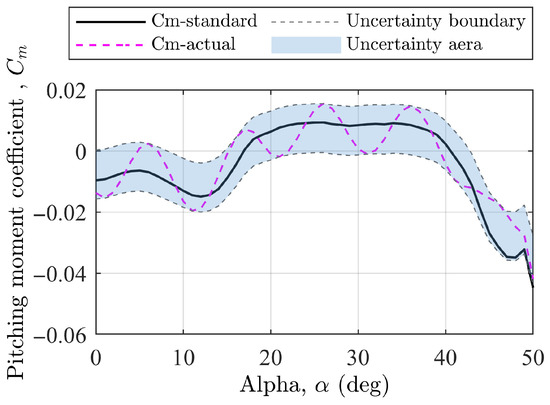
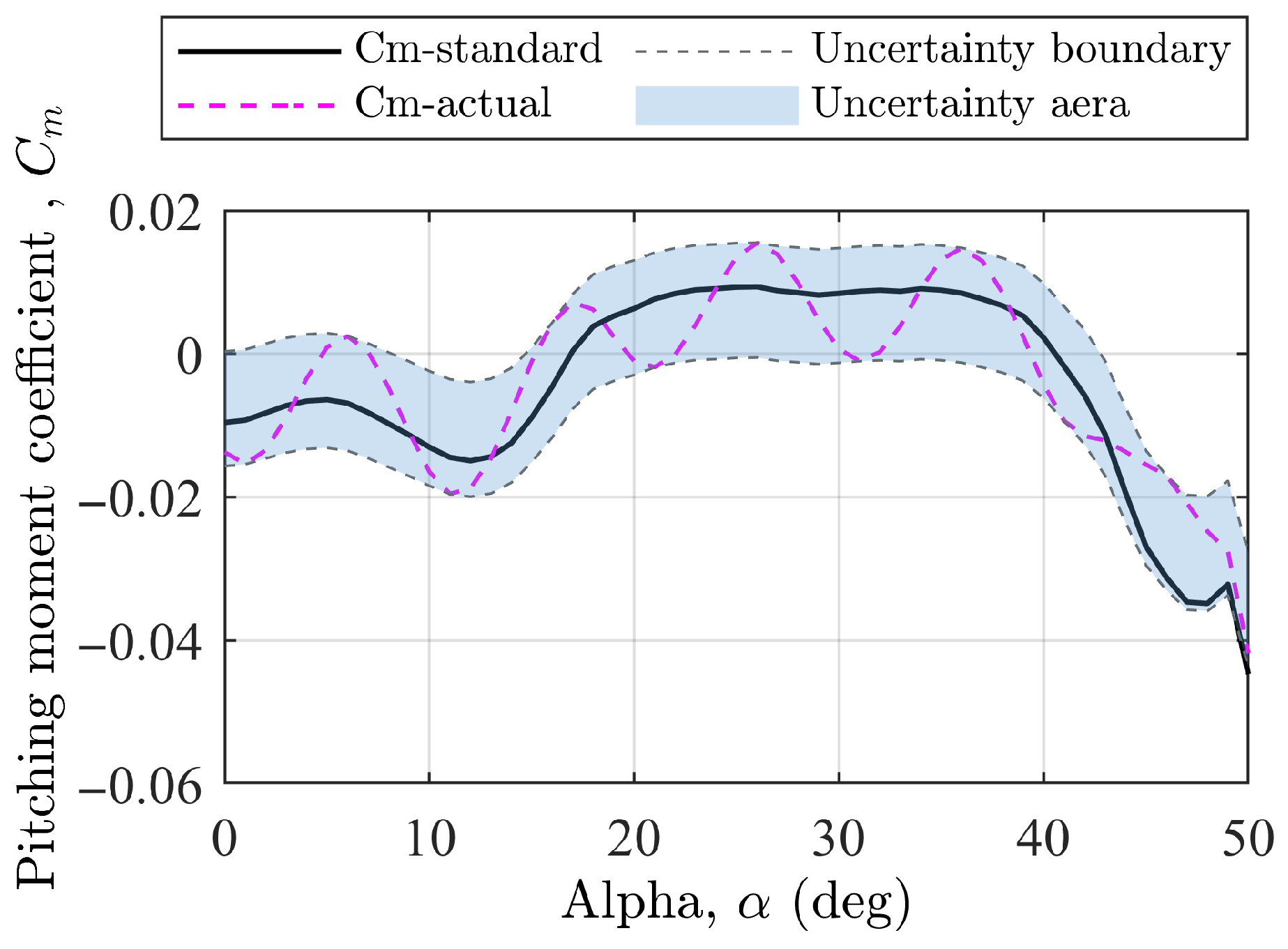
With respect to the design of model uncertainty, this study primarily considers uncertainties in aerodynamic parameters. Specifically, a small-amplitude sinusoidal perturbation is first superimposed on the three force coefficients and three moment coefficients, after which a uniform $20\%$ bias is applied to the aerodynamic parameters as a whole. Taking the pitching moment coefficient as an example, the actual pitching moment coefficient used in the simulation satisfies Equation (57). The sinusoidal perturbations applied to the six aerodynamic parameters are assigned different initial phases. The resulting model uncertainty in the pitching moment coefficient is illustrated in Figure 10.

$$\begin{array}{c}{C}_m\left(actual\right)=\left[C_m\left(standard\right)+\right.\left.0.01\ast \sin \left(\mathrm{pi}/5\ast \alpha +9\right)\right]·\left(1-20\%\right)\hfill \end{array}$$

(57)

Figure 10. Modeling of pitching moment coefficient uncertainty.

In the first two sets of simulations, constant control commands are applied. To further compare the responses of different control methods to time-varying commands, this section considers a trimmed level-flight condition as the initial flight state and introduces changes in the angle-of-attack and velocity-roll-angle commands during flight, while the sideslip-angle command is maintained at zero.

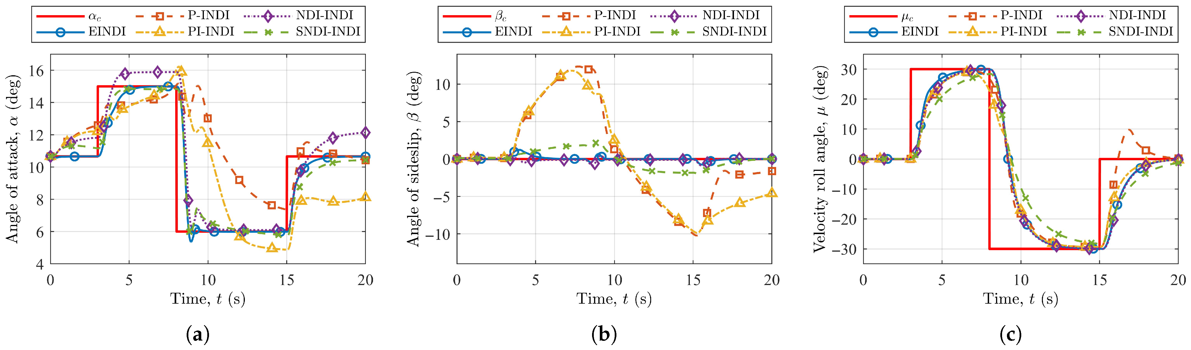
At the start of the simulation, the UAV is trimmed in level flight at an airspeed of 100 m/s with an angle of attack of 10.66 deg. At $t=3$ s, the angle-of-attack command is increased to 15 deg, and the velocity roll angle command is set to 30 deg. At $t=8$ s, the angle-of-attack command is changed to 6 deg, and the velocity roll angle command is set to −30 deg. Finally, at $t=15$ s, both the angle-of-attack and velocity roll angle commands are returned to their initial level-flight values.

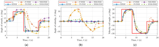
The simulation results obtained in the presence of model uncertainty are shown in Figure 11. Since all controllers employ the same INDI-based inner-loop design, only the time histories of the aerodynamic angles are presented. As illustrated in Figure 11a, owing to model uncertainty, NDI-INDI exhibits a pronounced steady-state error, which is even larger than that observed for SNDI-INDI. The linear outer-loop control laws show relatively slow responses when tracking rapidly varying command inputs and fail to follow the commands adequately within a limited time interval. This behavior indicates that linear outer-loop control approaches are unsuitable for flight missions with high maneuverability requirements. In contrast, EINDI is barely affected by model uncertainty and continues to demonstrate excellent response speed and control accuracy.

Figure 11. Time history of attitude angle tracking under model uncertainty using EINDI, P-INDI, PI-INDI, NDI-INDI and SNDI-INDI. (a–c) depict the time-domain evolution curves of angle of attack, sideslip angle and velocity roll angle, respectively.

Due to lateral–directional coupling, commands in the velocity roll angle induce deviations in the sideslip angle. Regarding sideslip angle regulation, as shown in Figure 11b, P-INDI and PI-INDI perform poorly in suppressing sideslip, with peak deviations reaching up to 13 deg. SNDI-INDI also produces sideslip oscillations of approximately 2 deg. By comparison, NDI-INDI results in smaller sideslip fluctuations, while EINDI exhibits superior performance in maintaining the sideslip angle close to zero. For velocity roll angle command tracking, the differences among the control methods are relatively minor, with only P-INDI showing a noticeably large overshoot.

The quantitative IAE and ITAE results are summarized in Table 6. It can be observed that, in the presence of model uncertainty, NDI-INDI still exhibits favorable performance in most aspects, with the exception of angle-of-attack control accuracy. For velocity roll angle tracking, the control performance is almost unaffected by system model errors. Although the performance of the linear outer-loop control strategies is significantly inferior to that of the other methods, they do not lead to loss of UAV control. This indicates that, within the attitude control loop, the availability of an explicit system model is not critically important, as this loop inherently possesses strong robustness. However, during highly dynamic maneuvering, accurate angle-of-attack control becomes essential. Near the limits of the UAV performance envelope, angle-of-attack tracking errors may easily cause the UAV to exceed the safe angle-of-attack boundary, which is clearly undesirable.

Table 6. IAE and ITAE results under model uncertainty.

Control Method and Index	$\mathit{\alpha }$	$\mathit{\beta }$	$\mathit{\mu }$	p	q	r
EINDI (IAE)	11.6	2.8	158.7	115.2	42.7	40.2
P-INDI (IAE)	43.1	98.9	156.3	138.7	25.7	13.0
PI-INDI (IAE)	45.5	11.9	154.4	118.0	37.8	13.1
NDI-INDI (IAE)	20.8	2.9	162.8	113.9	45.3	41.1
SNDI-INDI (IAE)	16.3	19.5	211.2	108.8	41.7	29.2
EINDI (ITAE)	101.5	21.7	1567.6	1136.7	413.2	366.6
P-INDI (ITAE)	405.9	1023.0	1471.2	1485.1	248.7	132.7
PI-INDI (ITAE)	504.3	1267.8	1444.2	1145.0	389.3	138.2
NDI-INDI (ITAE)	202.5	29.1	1587.5	1128.6	422.9	371.6
SNDI-INDI (ITAE)	156.2	208.8	2095.1	1101.2	409.9	260.0

It is worth noting an interesting phenomenon observed in Table 6: SNDI-INDI occasionally exhibits smaller steady-state error than NDI-INDI in $\alpha$-tracking under model uncertainty. This counterintuitive result reflects an important property of model-based dynamic inversion: when the onboard model is significantly biased, the use of a biased model in NDI-INDI actively injects a systematic error into the control loop, whereas SNDI-INDI—by omitting the model-based compensation altogether—avoids this contamination. In other words, in the presence of substantial model error, “no compensation” can be locally less harmful than “wrong compensation”. EINDI, by contrast, replaces the model-based compensation with sensor-derived information and thereby achieves the most favorable performance among the three nonlinear methods, neither omitting the compensation nor relying on a potentially biased model.

The simulation results in this subsection further demonstrate that, when model uncertainty is considered, the UAV attitude control loop itself exhibits strong robustness. Nevertheless, linear outer-loop control methods show poor sideslip suppression during lateral–directional maneuvers, whereas EINDI consistently maintains high control accuracy.

5. Conclusions

This paper proposed an EINDI control framework and applied it to the autonomous wing rock recovery problem of a low-aspect-ratio flying-wing UAV. The proposed approach introduces aerodynamic angular rate feedback into the outer-loop control design while retaining an INDI-based inner loop, thereby reducing the reliance on accurate system model information and improving attitude control accuracy.

Simulation studies were conducted using a full 6-DOF flight dynamics model of a low-aspect-ratio flying-wing UAV. The proposed controller was comparatively evaluated against linear outer-loop control, NDI-based outer-loop control, and a simplified NDI outer-loop control strategy. The results demonstrate that the EINDI framework is capable of achieving motion recovery from arbitrary initial states along the wing rock trajectory. Under nominal conditions, the control performance of EINDI is comparable to that of NDI-based control and superior to linear outer-loop designs in terms of tracking accuracy and smoothness. When model uncertainty is considered, the linear outer-loop control strategy exhibits poor sideslip suppression during lateral–directional maneuvers, while NDI-based approaches suffer from degraded angle-of-attack tracking accuracy. These findings indicate that the attitude control loop itself possesses strong inherent robustness; however, during highly dynamic maneuvers near performance limits, precise angle-of-attack regulation remains critical. In this context, the proposed EINDI framework provides improved angle-of-attack control performance under model uncertainty. In addition, the EINDI method proposed in this paper is applicable to fixed-wing unmanned aerial platforms equipped with aerodynamic-angle sensing capability.

Although the proposed method may impose increased requirements on sensor performance, this study demonstrates the effectiveness of aerodynamic angular rate feedback for controlling highly nonlinear and strongly coupled flight motions of flying-wing UAVs.

References

- Wang, H. Development of high performance collaborative combat UAVs. Acta Aeronaut. Astronaut. Sin. 2024, 45, 530304. (In Chinese) [Google Scholar] [CrossRef]
- Yang, W. Development of future fighters. Acta Aeronaut. Astronaut. Sin. 2020, 41, 524377. (In Chinese) [Google Scholar] [CrossRef]
- Wang, Y.; Bu, C.; Yang, W.; Shen, Y.; Feng, S. State-space representation of aerodynamica of flying wing with low aspect ratio at high angles of attack. Acta Aeronaut. Astronaut. Sin. 2021, 42, 124539. (In Chinese) [Google Scholar] [CrossRef]
- Wang, F.; Xie, K.; Liu, J.; Song, Y.; Qin, H.; Chen, L. Unsteady flow and wing rock characteristics of low aspect ratio flying-wing. Acta Aeronaut. Astronaut. Sin. 2023, 44, 126449. (In Chinese) [Google Scholar] [CrossRef]
- Wang, L.; Zhang, N.; Liu, H.; Yue, T. Stability characteristics and airworthiness requirements of blended wing body aircraft with podded engines. Chin. J. Aeronaut. 2022, 35, 77–86. [Google Scholar] [CrossRef] [Scilit]
- Katz, J. Wing/vortex interactions and wing rock. Prog. Aerosp. Sci. 1999, 35, 727–750. [Google Scholar] [CrossRef] [Scilit]
- Ma, B.; Deng, X.; Wang, B. Effects of wing locations on wing rock induced by forebody vortices. Chin. J. Aeronaut. 2016, 29, 1226–1236. [Google Scholar] [CrossRef] [Scilit]
- Geng, X.; Shi, Z.; Cheng, K. Experimental investigation of influence of strake wings on self-induced roll motion at high angles of attack. Chin. J. Aeronaut. 2016, 29, 1591–1601. [Google Scholar] [CrossRef] [Scilit]
- Li, X.; Feng, L.; Wang, Q. Wing Rock Mode and its Mechanism of a Flying-wing Aircraft. Flow 2023, 3, E38. [Google Scholar] [CrossRef] [Scilit]
- Jiang, Y.; Li, D.; Kan, Z.; Dong, B.; Zhen, C.; Xiang, J. Bifurcation analysis of wing rock and routes to chaos of a low aspect ratio flying wing. Nonlinear Dyn. 2024, 112, 21491–21508. [Google Scholar] [CrossRef] [Scilit]
- Nelson, R.C.; Pelletier, A. The Unsteady Aerodynamics of Slender Wings and Aircraft Undergoing Large Amplitude Maneuvers. Prog. Aerosp. Sci. 2003, 39, 185–248. [Google Scholar] [CrossRef] [Scilit]
- Yang, L.; Wu, J.; Tao, Y.; Ma, S.; Li, G.; Wu, J. Study on leading-edge vortex/shock interaction and unsteady characteristics of a transonic low-aspect-ratio flying wing. Phys. Fluids 2025, 37, 075220. [Google Scholar] [CrossRef] [Scilit]
- Hall, R.M.; Woodson, S.H.; Chambers, J.R. Overview of the abrupt wing stall program. Prog. Aerosp. Sci. 2004, 40, 417–452. [Google Scholar] [CrossRef] [Scilit]
- Guglieri, G. A comprehensive analysis of wing rock dynamics for slender delta wing configurations. Nonlinear Dyn. 2012, 69, 1559–1575. [Google Scholar] [CrossRef] [Scilit]
- Dong, Y.; Shi, Z.; Chen, K.; Yao, Z. Self-learned suppression of roll oscillations based on model-free reinforcement learning. Aerosp. Sci. Technol. 2021, 116, 106850. [Google Scholar] [CrossRef] [Scilit]
- Andrievsky, B.; Kudryashova, E.V.; Kuznetsov, N.V.; Kuznetsova, O.A. Aircraft wing rock oscillations suppression by simple adaptive control. Aerosp. Sci. Technol. 2020, 105, 106049. [Google Scholar] [CrossRef] [Scilit]
- Zribi, M.; Alshamali, S.; Al-Kendari, M. Suppression of the wing-rock phenomenon using nonlinear controllers. Nonlinear Dyn. 2013, 71, 313–322. [Google Scholar] [CrossRef] [Scilit]
- Mobayen, S.; Izadbakhsh, A. Observer-based suppression of the wing-rock oscillations using function approximation technique. Phys. Fluids 2025, 37, 017170. [Google Scholar] [CrossRef] [Scilit]
- Roshanian, J.; Rahimzadeh, E. Novel model reference adaptive control with application to wing rock example. Proc. Inst. Mech. Eng. Part G J. Aerosp. Eng. 2021, 235, 1911–1929. [Google Scholar] [CrossRef] [Scilit]
- Rong, H.; Han, S.; Zhao, G. Adaptive Fuzzy Control of Aircraft Wing-rock Motion. Appl. Soft Comput. 2014, 14, 181–193. [Google Scholar] [CrossRef] [Scilit]
- Capello, E.; Guglieri, G.; Sartori, D. Performance Evaluation of an L1 Adaptive Controller for Wing-Body Rock Suppression. J. Guid. Control Dyn. 2012, 35, 1702–1708. [Google Scholar] [CrossRef] [Scilit]
- Sun, W.; Wang, Y.; Pan, C.; Qi, Z. Delta wing rocking motion suppression by deep reinforcement learning. Phys. Fluids 2023, 35, 097125. [Google Scholar] [CrossRef] [Scilit]
- Kori, D.K.; Kolhe, J.P.; Talole, S.E. Extended state observer based robust control of wing rock motion. Aerosp. Sci. Technol. 2014, 33, 107–117. [Google Scholar] [CrossRef] [Scilit]
- Steinert, A.; Raab, S.; Hafner, S.; Holzapfel, F.; Hong, H. From fundamentals to applications of incremental nonlinear dynamic inversion: A survey on INDI—Part I. Chin. J. Aeronaut. 2025, 38, 103553. [Google Scholar] [CrossRef] [Scilit]
- Steinert, A.; Raab, S.; Hafner, S.; Holzapfel, F.; Hong, H. Advancements in incremental nonlinear dynamic inversion and its components: A survey on INDI—Part II. Chin. J. Aeronaut. 2025, 38, 103591. [Google Scholar] [CrossRef] [Scilit]
- Canin, D. F-35 High Angle of Attack Flight Control Development and Flight Test Results. In AIAA Aviation 2019 Forum; American Institute of Aeronautics and Astronautics: Dallas, TX, USA, 2019. [Google Scholar] [CrossRef] [Scilit]
- Chen, G.; Liu, A.; Hu, J.; Feng, J.; Ma, Z. Attitude and Altitude Control of Unmanned Aerial-Underwater Vehicle Based on Incremental Nonlinear Dynamic Inversion. IEEE Access 2020, 8, 156129–156138. [Google Scholar] [CrossRef] [Scilit]
- Acquatella, P.; Van Kampen, E.-J.; Chu, Q.P. A Sampled-Data Form of Incremental Nonlinear Dynamic Inversion for Spacecraft Attitude Control. In AIAA SCITECH 2022 Forum; American Institute of Aeronautics and Astronautics: San Diego, CA, USA, 2022. [Google Scholar] [CrossRef] [Scilit]
- Bose, D.; Hazra, A.; Mukhopadhyay, S.; Gupta, A. A Co-ordinated Control Methodology for Rapid Load-Following Operation of a Pressurized Water Reactor Based Small Modular Reactor. Nucl. Eng. Des. 2020, 367, 110748. [Google Scholar] [CrossRef] [Scilit]
- Salahudden, S. Decoupled Incremental Nonlinear Dynamic Inversion Control for Aircraft Spin Recovery. IEEE Trans. Aerosp. Electron. Syst. 2025, 61, 3336–3345. [Google Scholar] [CrossRef] [Scilit]
- Pfeifle, O.; Fichter, W. Cascaded Incremental Nonlinear Dynamic Inversion for Three-Dimensional Spline-Tracking with Wind Compensation. J. Guid. Control Dyn. 2021, 44, 1559–1571. [Google Scholar] [CrossRef] [Scilit]
- Wang, Z.; Zhao, J.; Cai, Z.; Wang, Y.; Liu, N. Onboard actuator model-based Incremental Nonlinear Dynamic Inversion for quadrotor attitude control: Method and application. Chin. J. Aeronaut. 2021, 34, 216–227. [Google Scholar] [CrossRef] [Scilit]
- Niestroy, M.A.; Dorsett, K.M.; Markstein, K. A Tailless Fighter aircraft Model for Control-Related Research and Development. In AIAA Modeling and Simulation Technologies Conference; American Institute of Aeronautics and Astronautics: Grapevine, TX, USA, 2017. [Google Scholar] [CrossRef] [Scilit]
- Stougie, J.; Pollack, T.; Van Kampen, E.-J. Incremental Nonlinear Dynamic Inversion control with Flight Envelope Protection for the Flying-V. In AIAA SCITECH 2024 Forum; American Institute of Aeronautics and Astronautics: Orlando, FL, USA, 2024. [Google Scholar] [CrossRef] [Scilit]
- Raghavendra, P.K.; Sahai, T.; Kumar, P.A.; Chauhan, M.; Ananthkrishnan, N. Aircraft Spin Recovery, with and without Thrust Vectoring, Using Nonlinear Dynamic Inversion. J. Aircr. 2005, 42, 1492–1503. [Google Scholar] [CrossRef] [Scilit]
- Wang, X.; Van Kampen, E.; Chu, Q.; Lu, P. Stability Analysis for Incremental Nonlinear Dynamic Inversion Control. J. Guid. Control Dyn. 2019, 42, 1116–1129. [Google Scholar] [CrossRef] [Scilit]
- Snell, S.A.; Enns, D.F.; Garrard, W.L. Nonlinear inversion flight control for a supermaneuverable aircraft. J. Guid. Control Dyn. 1992, 15, 976–984. [Google Scholar] [CrossRef] [Scilit]
Disclaimer/Publisher’s Note: The statements, opinions and data contained in all publications are solely those of the individual author(s) and contributor(s) and not of MDPI and/or the editor(s). MDPI and/or the editor(s) disclaim responsibility for any injury to people or property resulting from any ideas, methods, instructions or products referred to in the content. |
© 2026 by the authors. Licensee MDPI, Basel, Switzerland. This article is an open access article distributed under the terms and conditions of the Creative Commons Attribution (CC BY) license.