


Highlights
What are the main findings?
- A lightweight autonomous UAV navigation framework using only a single Intel RealSense D435i depth camera was developed for forest-like GNSS-denied environments, integrating RTAB-Map SLAM, direction-oriented frontier exploration, DWA-based local planning, and autonomous return-to-home.
- The proposed system achieved stable localization performance across low-, medium-, and high-density scenarios, with traversal RMSEs of 0.195, 0.197, and 0.420 m and return RMSEs of 0.295, 0.474, and 1.084 m, while also demonstrating effective real-time replanning and obstacle avoidance in dynamic environments.
What are the implications of the main findings?
- The results demonstrate that reliable UAV navigation in GNSS-denied and highly occluded environments can be achieved without heavy multi-sensor payloads, supporting lightweight platform design with reduced hardware complexity and power demand.
- The direction-oriented frontier strategy provides a practical exploration mechanism for directionally constrained environments such as forests, corridors, and warehouse passages, with potential applications in inspection, search and rescue, and autonomous exploration.
Abstract
In environments where GNSS signals are unavailable—such as indoor spaces, underground facilities, and forested areas—autonomous UAV navigation faces challenges related to localization uncertainty and limited onboard sensing capability. This study proposes a lightweight navigation framework using a single Intel RealSense D435i depth camera, integrating RTAB-Map SLAM, DWA-based local planning, and a direction-oriented frontier exploration strategy. The proposed exploration strategy introduces heading consistency into frontier target selection to support navigation in directionally constrained environments. The system is implemented within the ROS framework and evaluated in Gazebo/ArduPilot SITL simulation environments under low-, medium-, and high-density obstacle configurations. The results show that the system successfully completed autonomous traversal and return-to-home missions across all scenarios, with traversal RMSE values of 0.195 m, 0.197 m, and 0.420 m and return RMSE values of 0.295 m, 0.474 m, and 1.084 m, respectively. Qualitative dynamic-obstacle tests further demonstrate the system’s capability for local map updating and replanning. It should be noted that the current evaluation is primarily simulation-based and conducted in simplified environments. Therefore, the results are interpreted as initial system-level validation rather than full real-world deployment verification. The proposed system should not be directly interpreted as a ready-to-deploy real-world UAV navigation solution. Future work will focus on physical UAV experiments and more realistic GNSS-denied environments.
1. Introduction
1.1. Background
In recent years, Unmanned Aerial Vehicle (UAV) technology has advanced rapidly, extending its applications from military operations to civilian domains such as agricultural inspection, environmental monitoring, disaster search and rescue, and logistics delivery. However, most existing navigation methods remain highly dependent on the Global Positioning System (GPS). In highly occluded environments—including indoor spaces, underground facilities, and forested areas—satellite signals are prone to blockage and multipath effect interference, resulting in significant degradation of localization accuracy and potentially leading to navigation failure and mission interruption. Ensuring reliable autonomous navigation for UAVs in GNSS-denied environments has therefore emerged as a critical challenge in the field of autonomous flight.
To address this issue, many studies have adopted Simultaneous Localization and Mapping (SLAM) as an alternative approach, constructing environmental maps and estimating vehicle pose based on sensor inputs. While LiDAR-based or multi-sensor fusion systems can achieve high accuracy, they are often constrained in small UAV platforms by limitations in payload capacity, power consumption, and system complexity. Moreover, conventional frontier-based exploration strategies typically select the next exploration target according to either distance or information gain. Here, distance refers to the Euclidean distance between the robot’s current position and a candidate frontier point, and the system usually prioritizes the frontier with the shortest distance. Information gain, by contrast, is used to estimate the amount of unknown environmental information the robot can acquire after moving to that frontier, and is commonly evaluated by the quantity or area of the surrounding unexplored regions. However, such strategies generally emphasize distance minimization or information maximization while neglecting directional consistency in navigation, which can easily lead to path overlap and frequent turning during the exploration process.
In response to these challenges, this study proposes a lightweight autonomous navigation system that relies solely on a single Intel RealSense D435i depth camera. The system integrates real-time appearance-based mapping (RTAB-Map) SLAM with a direction-guided frontier exploration strategy to enable real-time mapping, dynamic obstacle avoidance, and autonomous return-to-home capability. The architecture is implemented within the ROS framework, combining move_base and MAVROS, and is validated across multiple scenarios using the Gazebo and ArduPilot SITL simulation environments. The focus of this study lies not only in constructing a navigation framework with minimal hardware requirements, but also in proposing a direction-oriented exploration mechanism to mitigate the oscillatory movements and repetitive path patterns that may arise in conventional frontier-based exploration strategies, thereby enhancing path continuity and navigation stability.
1.2. Contributions
The principal contributions of this study are summarized as follows:
- A lightweight single-sensor UAV navigation framework is developed using only an Intel RealSense D435i depth camera. The system integrates RTAB-Map SLAM, depth-based obstacle representation, DWA local planning, MAVROS-based flight control, and autonomous return-to-home functionality.
- A direction-oriented frontier exploration strategy is proposed to improve target selection stability in directionally constrained environments. The strategy incorporates heading consistency, costmap-based filtering, and failure-point exclusion mechanisms.
- A simulation-based evaluation is conducted in low-, medium-, and high-density forest-like environments. The system performance is assessed using localization RMSE, mission completion, robustness under different initial conditions, and qualitative dynamic-obstacle replanning behavior.
These contributions define the study as a simulation-based feasibility validation rather than a performance comparison study.
1.3. Related Work
1.3.1. Development of SLAM Techniques and Applications of RTAB-Map
Simultaneous localization and mapping (SLAM) constitutes a fundamental technology for mobile robots operating in unknown environments. Since the statistical framework was first proposed by Smith and Cheeseman [1], numerous algorithms have been developed, including GMapping [2], Hector SLAM [3], Cartographer [4], and the ORB-SLAM family [5], each introducing optimizations in areas such as loop closure detection, 2D/3D mapping, and feature matching.
Among these approaches, RTAB-Map performs loop closure detection based on appearance similarity and employs graph optimization to maintain global map consistency. Owing to its real-time performance and support for multiple sensor modalities, RTAB-Map has been widely adopted in indoor and outdoor autonomous navigation applications [6]. However, in environments with limited visual features or drastic lighting changes, RTAB-Map’s loop closure detection is easily disrupted, indicating that its performance remains sensitive to environmental conditions and dependent on certain parameter settings.
1.3.2. Sensor Selection and Advantages of Depth Cameras
Navigation accuracy is strongly influenced by sensor characteristics. LiDAR sensors provide high precision and long-range measurements but are often unsuitable for small UAV platforms due to their weight and power consumption constraints [7]. Stereo and RGB cameras offer low-cost alternatives; however, their localization reliability deteriorates in texture-poor or low-light environments [8,9]. In contrast, the Intel RealSense D435i depth camera is compact and lightweight, incorporates an onboard IMU, and exhibits robust performance under varying lighting conditions. It has therefore been extensively utilized in visual–inertial odometry (VIO) and dynamic obstacle tracking applications [10,11,12]. Previous studies have further demonstrated that IMU integration can significantly enhance the stability of RTAB-Map localization and mapping [13]. Consequently, the D435i represents a practical compromise between lightweight design and operational robustness.
1.3.3. Path Planning and Exploration Strategies
Conventional frontier-based exploration methods typically select exploration targets based on information gain or shortest-path criteria [14,15]. While effective in promoting exploration of unknown regions, these approaches often result in redundant path traversal and discontinuous navigation directions, thereby reducing global exploration efficiency. Some studies have incorporated cost maps or heuristic strategies to mitigate exploration redundancy [16]; however, they generally lack designs tailored to environments with strong directional constraints, such as forest corridors or elongated passageways. This limitation suggests that existing exploration strategies remain suboptimal in directionally structured environments.
1.3.4. Research Gap and Positioning of This Study
A synthesis of the above literature reveals several key observations:
- Although SLAM technologies have matured considerably, their performance remains highly dependent on environmental features, with limited optimization specifically targeting highly occluded environments.
- Multi-sensor fusion can improve robustness but increases system complexity and payload demands, which conflict with the lightweight requirements of small UAV platforms.
- Existing frontier exploration strategies largely overlook directional consistency in navigation, resulting in reduced efficiency in forested or elongated environments.
In response to these gaps, this study proposes a single-camera navigation architecture that integrates RTAB-Map SLAM with a direction-oriented frontier exploration strategy to reduce hardware complexity while improving target selection stability. The proposed design is positioned as a simulation-based feasibility validation for highly occluded and directionally constrained scenarios, such as simplified forest-like traversal, rather than as a complete real-world deployment verification.
Therefore, the main objective of this study is to validate the feasibility of a lightweight UAV navigation framework for GNSS-denied environments using only a single Intel RealSense D435i depth camera.
Specifically, this study evaluates whether such a single-sensor configuration can support autonomous traversal, SLAM-based localization, obstacle avoidance, direction-oriented exploration, and return-to-home navigation under different obstacle-density conditions.
Accordingly, the central research question is formulated as follows:
Can a UAV equipped with a single depth camera achieve stable autonomous navigation, as evaluated by localization accuracy, mission completion, and obstacle avoidance behavior, in GNSS-denied environments under varying obstacle-density conditions?
This question is examined through simulation-based experiments.
2. System Architecture and Methodology
2.1. System Overview
This study develops an autonomous UAV navigation system designed for operation in unknown environments. The system is formulated on a two-dimensional navigation framework and provides real-time mapping, autonomous localization, dynamic obstacle avoidance, and return-to-home capabilities. To address the challenges associated with navigation in GNSS-denied environments, the architecture integrates modules for environmental sensing, map construction, path planning, and flight control. The overall system is validated and evaluated within the Gazebo simulation platform.
In the present implementation, the navigation problem is formulated as a fixed-altitude planar navigation task. The mapping, frontier selection, and local planning modules operate on a two-dimensional occupancy-grid representation.
The UAV altitude is maintained at a predefined constant height, while roll and pitch are stabilized by the flight controller. Therefore, the system should not be interpreted as a full three-dimensional aerial navigation solution.
Although the system is primarily developed and integrated in a simulated environment, the validity of the sensor model is first established to ensure the realism of simulation results. Specifically, depth data generated by the physical camera and the simulated camera are compared under static conditions to verify output consistency. This comparison confirms the accuracy and reliability of the simulated camera model, which subsequently serves as the foundation for navigation system development and testing. The system integrates multiple development and simulation components, including computing platforms, simulation tools, physical sensors, and software frameworks.
The development platform consists of an MSI Vector GP 78 HX 13V series laptop (Micro-Star International Co., Ltd., New Taipei City, Taiwan) equipped with an Intel® Core™ i9 processor (Intel Corporation, Santa Clara, CA, USA), 32 GB of memory, and an NVIDIA® GeForce RTX™ 4080 Laptop GPU (NVIDIA Corporation, Santa Clara, CA, USA). The host operating system is Windows 11, and an Ubuntu 20.04 LTS environment is deployed via VMware Workstation 17 Pro virtualization software as the primary platform for development and experimentation.
The simulation environment is based on Gazebo 11, a three-dimensional simulator featuring a real-time physics engine and multi-sensor simulation capabilities for modeling aerial vehicle dynamics and environmental interactions. The UAV platform utilizes a quadrotor model provided by IQ Sim [17], which includes the base_link frame, rotor structures, and an inertial measurement unit (IMU), and supports integration with ArduPilot Software-In-The-Loop (SITL) version 4.0.4. To emulate realistic sensing outputs, the realsense_ros_gazebo package [18] is incorporated to simulate the Intel RealSense D435i depth camera, including RGB imagery, depth maps, and IMU data, thereby closely approximating real-world sensor inputs.
For physical validation, experiments are conducted using the same Intel RealSense D435i depth camera employed in the simulation. This device utilizes stereo vision combined with infrared projection for depth sensing and integrates a six-axis IMU. The relevant hardware specifications are summarized in Table 1.
Table 1.
Specifications and experimental settings of the Intel RealSense D435i camera.
The Intel RealSense D435i was selected because it provides a suitable balance between payload constraints and sensing capability for lightweight UAV navigation. The camera is compact and lightweight, weighing approximately 75 g, and integrates RGB-D sensing with a six-axis IMU.
Its wide field of view, short-to-medium operating range, ROS compatibility, and availability in Gazebo simulation make it suitable for integration with RTAB-Map and the proposed navigation framework.
The camera also provides sufficient frame rate for real-time SLAM and local planning.
However, its robustness in outdoor environments with strong lighting variation or adverse conditions is limited and is not fully evaluated in the current study. Therefore, it is not claimed to be the optimal sensing solution, but rather a practical trade-off among sensing capability, weight, cost, and integration complexity.
The system software is centered on the ROS framework, which serves as the integration core responsible for data management and inter-module communication through topic exchange. Flight control is simulated using ArduPilot SITL, which emulates the onboard flight controller. Communication between ROS and the SITL environment is established via the MAVROS package (ROS Noetic compatible release), enabling flight mode switching, position control, and status feedback.
For the navigation subsystem, RTAB-Map is employed as the visual SLAM framework for map construction and localization. The depthimage_to_laserscan package [19] is incorporated to convert depth images into laser scan representations compatible with move_base [20]. Path planning is performed using the Dynamic Window Approach (DWA) algorithm to support real-time obstacle avoidance and local navigation. An in-house developed control node is implemented to execute UAV flight control and navigation commands.
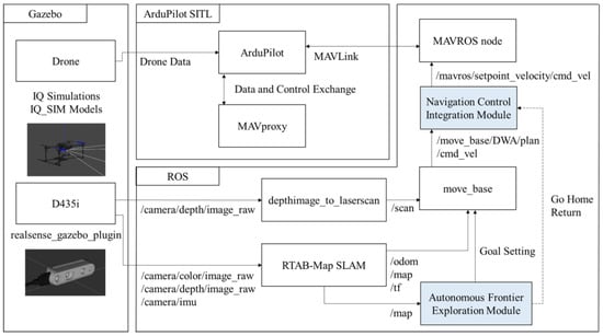
To realize a complete navigation pipeline, the proposed autonomous UAV navigation system is organized as illustrated in Figure 1 and divided into three principal modules:
Figure 1.
Integrated system architecture diagram (blue blocks denote custom-developed module nodes).
- Simulation environment and sensor data generation: The Gazebo simulation platform provides real-time depth imagery and UAV motion information.
- Flight control simulation and communication bridging: ArduPilot SITL emulates the flight controller, while MAVROS enables seamless integration with ROS.
- Sensor processing and navigation control module: RTAB-Map, move_base, and custom-developed nodes are deployed to achieve real-time mapping, obstacle avoidance, and navigation control.
2.2. RTAB-Map SLAM Integration
RTAB-Map is a graph-optimization-based SLAM framework proposed by Labbé and Michaud [21]. Its central concept is to represent environmental observations as a node–edge graph structure and to perform loop closure detection based on appearance similarity in order to correct accumulated drift caused by sensor errors. Compared with other SLAM approaches, RTAB-Map offers real-time processing capability, sensor flexibility—supporting RGB-D cameras, stereo vision, 3D LiDAR, and external odometry—and a hierarchical memory management mechanism, enabling stable operation in long-duration and large-scale navigation tasks.
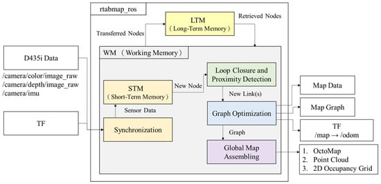
The overall workflow, illustrated in Figure 2, can be summarized in five stages:
Figure 2.
Schematic diagram of the RTAB-Map architecture and operational workflow within the ROS framework [6].
- Data acquisition and node creation: The system continuously receives RGB-D and IMU data and performs coordinate transformations through the TF framework to ensure that all sensor measurements are integrated within a unified reference frame. After processing in Short-Term Memory (STM), a new node is created that encapsulates pose estimation results, visual features, and depth information, forming the basis for subsequent matching and optimization.
- Visual odometry and spatial transformation: During node creation, visual odometry (VO) is employed to estimate the relative pose between consecutive nodes and to establish odometry edges. RTAB-Map supports two operating modes: (1) Frame-to-Frame (F2F), which computes relative motion by matching features between adjacent images, providing real-time performance but being susceptible to cumulative drift; and (2) Frame-to-Map (F2M), which matches the current frame against map nodes to reduce drift at the expense of higher computational cost. These modes can be alternated as required to balance accuracy and efficiency.
- Loop closure and proximity detection: To mitigate long-term accumulated errors, loop closure and proximity detection are performed within Working Memory (WM). Node images are first converted into Bag-of-Words (BoW) histograms to enable rapid retrieval of appearance similarity with historical nodes. When a similarity threshold is exceeded, geometric verification is conducted to ensure spatial consistency. If loop closure is not established, proximity detection compensates for cases in which feature scarcity limits recognition.
- Graph optimization: When new edges—arising from odometry, loop closure, or proximity constraints—are added, graph optimization is triggered to adjust the relative poses among nodes, ensuring global map consistency and convergence. The optimized graph is then forwarded to the global map assembly module, which generates map data, the map graph structure, and coordinate transformations (e.g.,/map →/odom) for use by the navigation subsystem.
- Memory management: RTAB-Map employs a hierarchical memory architecture to support long-term operation: (1) STM stores the most recent observations; (2) WM retains recently active nodes for real-time matching; and (3) Long-Term Memory (LTM) archives historical nodes on disk and reloads them when necessary. This strategy reduces memory overhead and improves loop closure efficiency, enabling stable performance in large-scale environments.
RTAB-Map has been widely applied in autonomous robotics and UAV navigation, offering advantages such as high sensor integration capability, robust loop closure detection, and suitability for long-term operation. However, its performance is strongly influenced by scene feature distribution and parameter configuration. In environments with sparse visual features or abrupt illumination changes, the accuracy of loop closure detection may deteriorate. In this study, RTAB-Map is selected as the core mapping module primarily due to its high compatibility with the ROS framework and its ability to provide stable real-time localization in GNSS-denied environments.
2.3. Local Path Planning with Dynamic Window Approach (DWA)
The Dynamic Window Approach (DWA), proposed by Fox et al. [22], is a velocity-space-based local path planning method. Unlike traditional waypoint-based planning techniques, DWA directly searches for optimal velocity commands in the control space and makes decisions through short-term trajectory simulation combined with an evaluation function. This approach simultaneously accounts for real-time responsiveness, obstacle avoidance, and the dynamic constraints of the robot, making it particularly well-suited for real-time autonomous navigation.
For nonholonomic mobile platforms, the motion model is described by Equation (1):
where denotes the current position, represents the heading angle, and and correspond to the linear and angular velocities, respectively.
In velocity space, the DWA considers only the set of velocity commands that are reachable within a finite time horizon, as defined in Equation (2):
Here, , denotes the current velocity state, , represents the maximum linear and angular accelerations, respectively, and is the simulation time interval used in the DWA algorithm.
Within the dynamic window, each candidate velocity pair (v, ω) is subjected to trajectory simulation and evaluated using the objective function defined in Equation (3):
where path_distance(v,ω) evaluates the alignment between the simulated trajectory and the global path, represents the proximity of the trajectory endpoint to the target position, and obstacle_cost reflects the distance between the trajectory and surrounding obstacles based on the costmap.
In this study, the weighting coefficients in Equation (3) correspond directly to the ROS DWA parameters as follows:
The numerical values used in this work are:
These coefficients determine the trade-off between path-following behavior, goal-directed motion, and obstacle avoidance. A higher value of α encourages the UAV to remain closer to the global path, while β increases the priority of reaching the goal. The parameter γ penalizes trajectories that approach obstacles, thereby improving navigation safety.
It should be noted that, unlike the original DWA formulation, which includes heading, clearance, and velocity terms, the ROS-based implementation used in this study adopts path distance, goal distance, and obstacle cost as evaluation criteria. Therefore, the velocity term is not explicitly included in the objective function, but is implicitly constrained by the dynamic window and velocity limits.
- Heading function : This function computes the angular deviation between the terminal heading of the simulated trajectory and the direction of the target. A smaller deviation corresponds to a higher score, as expressed in Equation (4):
- Clearance function : This function evaluates the minimum distance between all points along the simulated trajectory and surrounding obstacles. A larger minimum distance indicates a safer trajectory, as defined in Equation (5):
- Velocity function : This term encourages faster motion by assigning a score proportional to the linear velocity , as shown in Equation (6):
Here, are weighting coefficients used to balance directional alignment, safety, and velocity requirements during navigation. The velocity pair that maximizes is selected as the control output for the current cycle.
A principal advantage of DWA lies in its explicit incorporation of the vehicle’s kinematic and dynamic constraints, enabling rapid adaptation to environmental changes and making it well-suited for highly uncertain and dynamic scenarios. Nevertheless, the method has inherent limitations. First, it is highly sensitive to the reliability of map and sensor data; excessive sensing noise may lead to erroneous planning decisions. Second, as a local planner, DWA often becomes trapped in local minima due to its lack of a global perspective, particularly in environments such as U-shaped obstacles, and therefore cannot guarantee a globally optimal path. Accordingly, the innovation of this study lies in integrating a direction-guided frontier exploration strategy, enabling the UAV to maintain a more consistent motion direction during exploration and thereby reducing the unstable navigation behavior caused by local minima in the DWA objective function.
2.4. Direction-Oriented Frontier Exploration
2.4.1. Exploration Strategy Design
The proposed direction-oriented frontier exploration strategy is designed to improve target selection stability in directionally constrained environments.
In conventional frontier-based exploration, targets are typically selected based on distance or information gain. However, in forest-like or corridor-like environments, such strategies may result in frequent heading changes, redundant path traversal, and unstable navigation behavior.
A frontier is defined as the boundary between known free space and unexplored regions and serves as a candidate target for exploration.
In this study, directional consistency is introduced as a preference rather than a strict constraint. Infeasible targets are filtered using the costmap, and unreachable targets are recorded and excluded from future selection.
Recovery behaviors, including map clearing, rotation, and backward motion, are applied to avoid deadlock situations. This mechanism prevents repeated selection of infeasible targets and reduces the risk of local trapping.
- Frontier detection and filtering: The system first extracts all frontier candidate points and applies a series of filtering rules to improve navigation efficiency and success rate:
- Candidate points located too close to the previously selected target are discarded to prevent redundant attempts.
- Points situated within obstacles or high-risk regions are excluded based on costmap evaluation.
- Regions previously associated with navigation failures and recorded in a failure list are removed from consideration.
- 2.
- Direction-guided prioritization: A preferred exploration direction may be predefined by the operator, such as due north (0°), northeast (45°), or northwest (330°). Candidate frontier points are ranked according to their alignment with a directional vector, and the point most consistent with the desired heading is selected as the navigation target. This mechanism is particularly suitable for directionally constrained scenarios, such as forest traversal or corridor inspection.
- 3.
- Target dispatch and navigation execution: The filtered navigation target is transmitted to the move_base module, which performs path planning and motion control. Upon reaching the target, the system reinitiates the frontier detection process, iteratively advancing the exploration task.
- 4.
- Failure recovery mechanism: When the UAV is unable to reach the designated target, the system executes the following recovery actions in sequence:
- Clearing the local costmap.
- Performing an in-place rotation to expand the sensing field of view and trigger the generation of new frontier points.
- Moving backward for two seconds at an estimated speed of 0.5 m/s to ensure sufficient clearance from nearby obstacles.
- 5.
- Return-to-home conditions: The system automatically switches to return-to-home mode under the following conditions:
- No valid frontier points remain on the map.
- The UAV exceeds a predefined distance threshold of 30 m from the starting position, which can be adjusted according to mission requirements.
2.4.2. Exploration Process
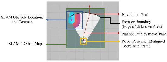
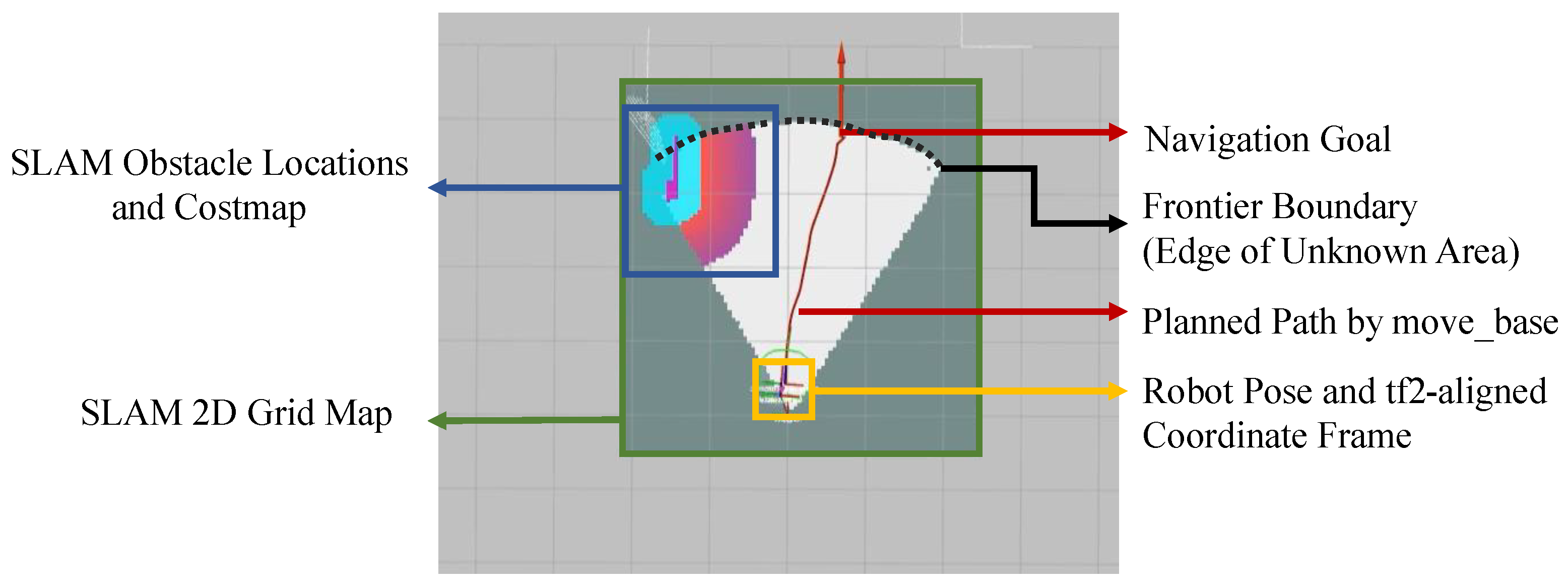
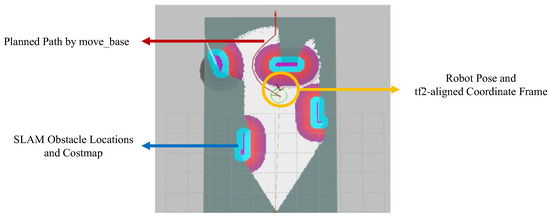
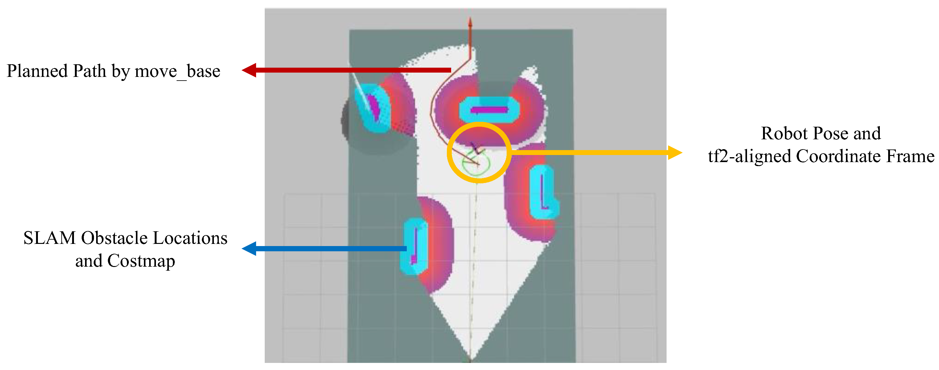
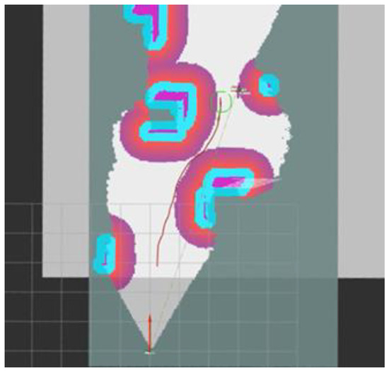
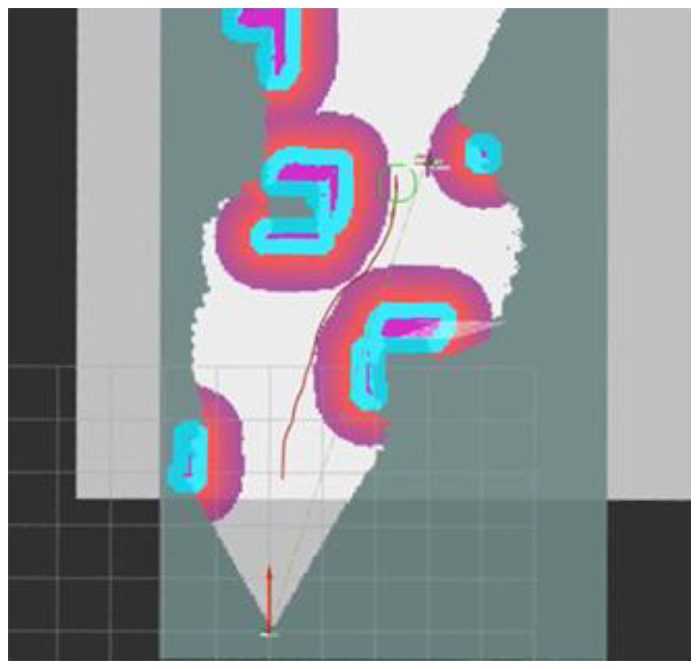
To provide a clearer illustration of the operational behavior of this module, Figure 3, Figure 4 and Figure 5 depict the exploration process at different stages:
Figure 3.
Selection of a northern frontier target point for navigation.
Figure 4.
Automatic updating of target points and obstacle-avoidance paths.
Figure 5.
Execution of the return-to-home mechanism using the starting position as the navigation target.
- Initial exploration stage: Within the two-dimensional grid map constructed by the SLAM system, the controller selects a frontier located in the northern direction and sufficiently distant from obstacles as the initial navigation target. A feasible local path is then generated toward this target, as illustrated in Figure 3. The blue box denotes the SLAM obstacle locations and costmap; the red arrow and line represent the navigation goal and the planned path generated by move_base, respectively; the black dashed line indicates the frontier boundary (the edge of the unknown area); the yellow box marks the UAV position; and the green box corresponds to the SLAM 2D grid map.
- Intermediate exploration stage: After the UAV reaches the current target, the system reanalyzes the frontier distribution based on the updated map and automatically selects the next navigation objective, generating a new path accordingly. This iterative process enables continuous exploration without requiring a preconstructed global map, as illustrated in Figure 4.
- Exploration completion and return-to-home: When the mission termination conditions are satisfied—such as exceeding a predefined travel distance or the absence of available frontier points—the system automatically designates the starting position as the return target. The path planner then computes a safe return trajectory that avoids environmental obstacles, thereby completing the mission, as illustrated in Figure 5.
2.5. Navigation and Return-to-Home Control
To ensure that the UAV can safely return to its starting point upon completion of exploration, an automatic return-to-home module is developed. When the return condition is triggered, the system designates the initial position (0, 0) as the navigation target and transmits it to the move_base module for path planning and execution. During the return process, RTAB-Map SLAM continuously updates the map, enabling the planner to avoid newly detected obstacles in real time.
The navigation control module receives velocity commands from the/cmd_vel topic, transforms them into the vehicle’s body coordinate frame via TF, and encapsulates them through MAVROS as/mavros/setpoint_velocity/cmd_vel. These commands are then executed by the ArduPilot SITL controller to perform flight control. If no feasible path is available during the return phase, the system automatically invokes the same recovery mechanisms used during exploration, repeating them as necessary until the return is successfully completed.
In addition, the control module supports several specialized commands, including rotate, backward motion, map clearing, return-to-home, and stop. These behavioral commands temporarily override the standard navigation controller and automatically revert to normal operation upon completion, thereby ensuring stable performance throughout both exploration and return phases.
3. Experimental Setup and Evaluation
3.1. Simulation Environment and UAV Configuration
To evaluate the UAV’s capabilities in mapping, obstacle avoidance, and return-to-home operations within unstructured environments such as forests, a simulation environment measuring approximately 30 × 30 m (total area 900 m2) was constructed in Gazebo. The base map was derived from the CCO-VOXE project released by Harithas et al. on GitHub [23] (accessed on 8 July 2025). This Box Cylinder World scenario features a forest-like layout populated with diverse obstacles and is well-suited for complex environment simulation. While preserving the original characteristics of the scene, two primary modifications were introduced: (1) reconfiguration of obstacle quantity and density, and (2) integration of a quadrotor UAV model equipped with a D435i camera for subsequent validation.
The simulation scenarios are designed as simplified forest-like environments composed of geometric obstacles (e.g., cubes and cylinders) with controlled density levels.
Although these scenarios allow repeatable evaluation, they do not fully reproduce real forests, such as irregular trunks, branches, foliage, canopy structures, uneven terrain, dynamic lighting, and partial occlusions.
To investigate navigation performance under varying forest densities, three representative scenarios—low, medium, and high density—were designed. Because the simulated environment does not include foliage or canopy structures, classifying density solely by obstacle count would not adequately represent actual occlusion conditions. Therefore, this study adopts the Ground Trunk Coverage Ratio (GCR) and equivalent tree density (trees per ha) as primary density metrics, supplemented by an analysis of navigable passage width.
The GCR is defined in Equation (7):
where represents the base area of the -th obstacle and denotes the total map area of 900 m2.
For comparison with conventional forestry density classification methods, the equivalent tree density of each scenario is also computed, as defined in Equation (8):
where N denotes the total number of obstacles and represents the map area.
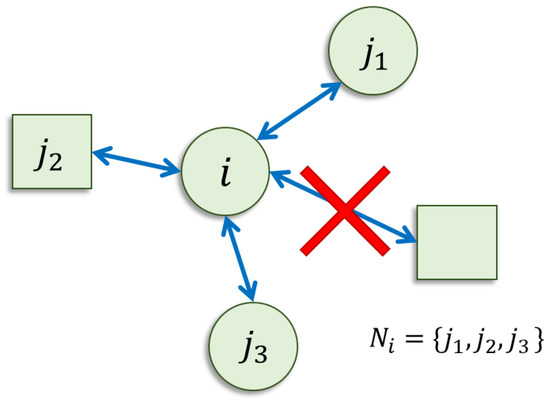
The local navigable spacing is defined as the center-to-center distance between obstacle iii and obstacle , minus their respective radii and , yielding the effective traversable width . This relationship is expressed in Equation (9):
and its geometric definition is illustrated in Figure 6.
Figure 6.
Schematic illustration of local navigable spacing calculation.
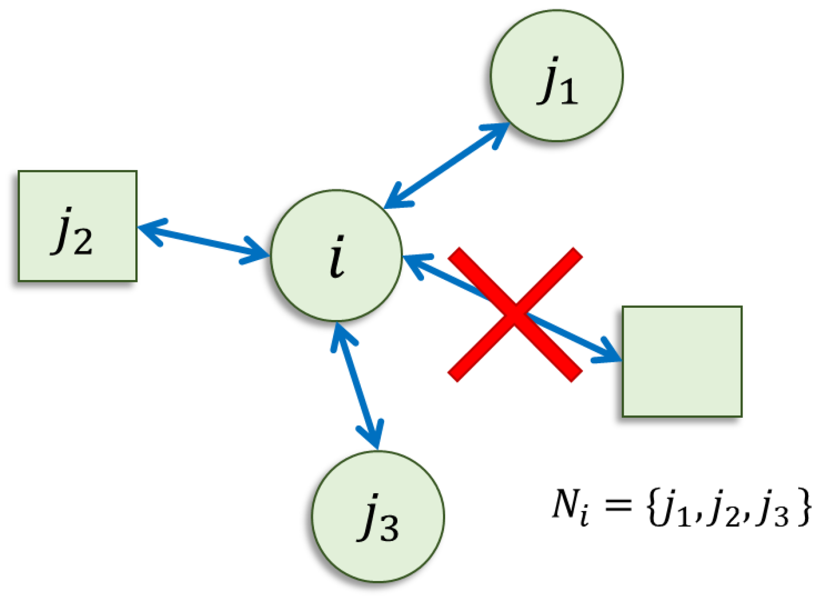
To ensure a representative characterization of local inter-obstacle spacing, the analysis considers, for each obstacle , only its three nearest neighboring obstacles . The average traversable width , as well as the minimum and maximum traversable widths , are computed accordingly, as defined in Equation (10):
A schematic illustration of this definition is presented in Figure 7, where the red cross denotes a neighboring obstacle excluded from the calculation because it is not among the three nearest neighbors.
Figure 7.
Schematic illustration of average traversable width calculation.
The obstacles used in the simulation are categorized into three types: large cubes, small cubes, and cylinders. Their dimensions and base areas are listed in Table 2, while the quantity distribution and statistical results for the three scenarios are summarized in Table 3. The results indicate GCR values of 7.01%, 10.98%, and 14.59%, corresponding to equivalent tree densities of 277.78, 455.56, and 611.11 trees/ha, respectively, with consistent proportional scaling across density levels.
Table 2.
Dimensions and base areas of tree obstacles.
Table 3.
Obstacle configuration and ground coverage statistics for different scenarios.
As obstacle density increases, the average traversable width decreases from 3.868 m to 2.607 m, with a minimum width of approximately 1.5 m. This value approaches the UAV’s wheelbase-equivalent span and turning radius, indicating that high-density scenarios substantially increase the complexity of obstacle avoidance and path planning.
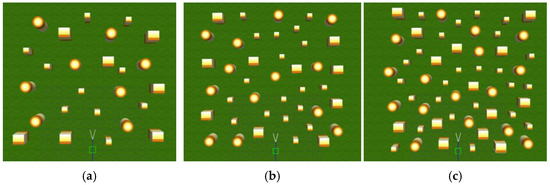
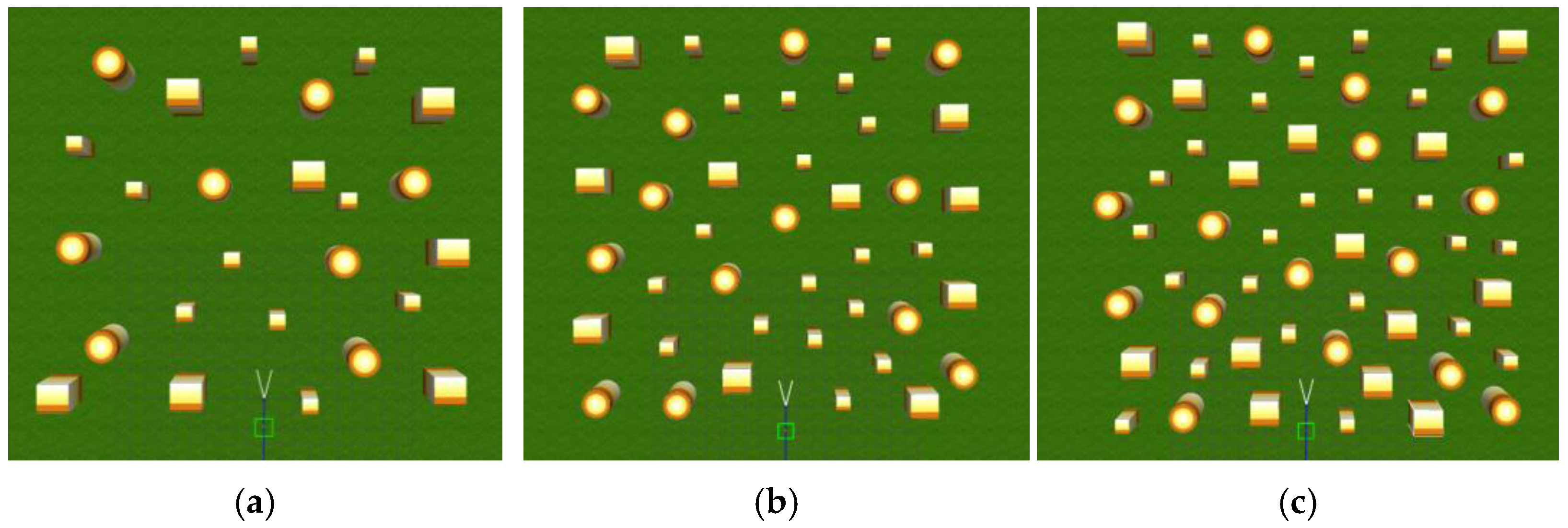
As illustrated in Figure 8, the low-, medium-, and high-density scenarios exhibit obstacle distributions ranging from sparse to highly compact. It is noteworthy that although individual small obstacles occupy a limited area, their dense arrangement in high-density environments produces substantial occlusion and increased navigation difficulty. Prior studies have likewise indicated that higher levels of occlusion can adversely affect SLAM loop closure detection and localization stability [24]. Accordingly, this study employs three quantitative indicators—GCR, equivalent tree density, and traversable passage width—to construct representative simulation scenarios that serve as a consistent evaluation framework for subsequent system validation and comparison.
Figure 8.
Gazebo simulation environments with cylindrical and cuboid obstacles: (a) low-density map; (b) medium-density map; (c) high-density. The green marker represents the UAV reference position in Gazebo.
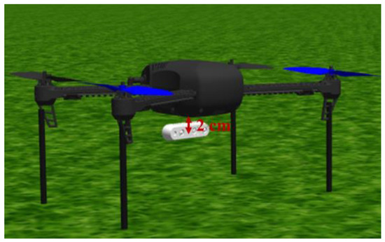
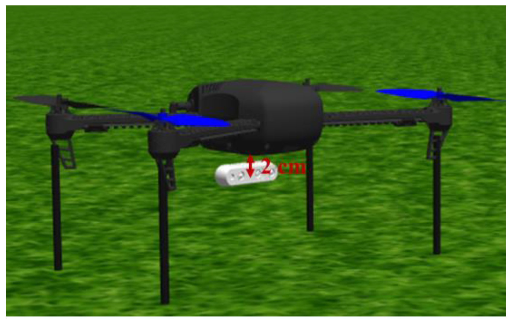
A quadrotor UAV model is deployed in the simulation platform (IQ Sim standard airframe, with an approximate diagonal wheelbase of 420 mm) and is equipped with an Intel RealSense D435i depth camera mounted at the front of the vehicle. The camera is installed at a height of approximately 2 cm and oriented horizontally in the forward direction, as shown in Figure 9. Through the realsense_ros_gazebo package, the camera provides RGB-D and IMU data, which are transformed into the UAV body coordinate frame via the ROS TF framework to ensure consistency in mapping and navigation.
Figure 9.
Gazebo quadrotor UAV equipped with a D435i camera.
This configuration approximates the basic RGB-D and IMU sensing inputs of a D435i-equipped UAV in a controlled GNSS-denied simulation environment. However, it does not fully reproduce real-world disturbances such as sunlight interference, vibration, motion blur, foliage occlusion, or dynamic lighting. Therefore, the simulation results are interpreted as initial system-level validation rather than complete real-world performance verification.
3.2. SLAM and Navigation Workflow
The navigation system is integrated within the ROS Noetic framework and comprises modules for sensor input, SLAM-based mapping, path planning, and flight control. The SLAM component employs RTAB-Map to perform simultaneous localization and mapping by fusing depth imagery and IMU data. To support path planning, depth images are converted into laser scan representations using the depthimage_to_laserscan package for compatibility with move_base. Local path planning is implemented using the DWA algorithm to enable real-time obstacle avoidance.
In addition, a direction-oriented frontier exploration strategy is developed to enhance navigation stability and exploration efficiency. By prioritizing frontier points aligned with the principal heading and incorporating failure-point filtering together with local costmap analysis, the system improves target selection robustness. Selected navigation goals are transmitted to move_base for execution. If navigation fails, recovery behaviors—such as map clearing, in-place rotation, or backward motion—are automatically triggered.
3.3. System Frequency and Velocity Constraints
The operational frequencies of each system module and sensor are presented in Table 4.
Table 4.
Operational frequencies of system modules.
Among them, RTAB-Map is capable of updating at only 1 Hz, resulting in an end-to-end sensing-to-planning latency of approximately . To ensure safe UAV operation within this latency interval, both velocity and acceleration must be appropriately constrained. First, based on the stable depth sensing range of the D435i camera, defined as , the maximum allowable linear velocity can be derived, as expressed in Equation (11):
Furthermore, to prevent insufficient visual overlap between consecutive sensor frames, the horizontal field of view of the D435i depth camera (FOV = 87°) was considered. A conservative safe disparity angle of ° ≈ 0.7 rad was therefore specified. In conjunction with the same latency duration, the maximum allowable angular velocity can be derived, as formulated in Equation (12):
Within the ROS/MAVROS framework, velocity control commands are updated at approximately 4 Hz (control interval s). Assuming that the UAV can accelerate from rest to and within a single control cycle, the corresponding linear acceleration and angular acceleration can be derived as expressed in Equations (13) and (14), respectively.
Accordingly, in the experimental implementation, the UAV’s linear and angular velocities were constrained to and , respectively, in order to ensure navigation stability and operational safety under sensing latency conditions.
3.4. Mission Design and Evaluation Metrics
The camera range and system latency were considered when defining conservative velocity constraints for the UAV. These constraints ensure stable perception and safe obstacle avoidance under sensing and processing limitations.
- Depth sensor validation: A comparative analysis was conducted to assess the consistency between simulated and physical D435i depth outputs.
- Multi-Scenario navigation tests: Traversal and return missions were executed in low-, medium-, and high-density environments, with localization performance quantified using the Root Mean Square Error (RMSE).
- Initial condition robustness Tests: The starting position and exploration direction were varied to examine navigation stability and fault tolerance under differing initial configurations.
- Dynamic obstacle tests: Sudden obstacles were introduced during navigation to evaluate real-time obstacle avoidance and replanning capabilities.
3.5. Data Collection and Analysis
Experimental data were recorded using ROS bag, including camera images, depth maps, IMU measurements,/odom and/tf coordinate information,/cmd_vel control outputs, and the planning results generated by move_base.
The data analysis procedure was conducted as follows:
- Localization error computation: The/map coordinates produced by the SLAM system were compared against known GPS ground truth or simulated reference values to calculate the RMSE.
- Navigation performance validation: Navigation and return performance under varying environmental densities were evaluated through RMSE analysis, complemented by visualization results in RViz and Gazebo.
- Obstacle avoidance and replanning assessment: The system’s response latency and path replanning success rate were analyzed when dynamic obstacles were introduced during navigation.
Through the above experimental design, the proposed navigation framework was comprehensively validated within a simulated environment, demonstrating its feasibility and robustness across diverse operational scenarios.
4. Experimental Results and Analysis
4.1. Depth Accuracy Comparison
To validate the credibility of the Intel RealSense D435i model in the Gazebo simulation environment, a two-stage experimental procedure was designed. The first stage evaluated the stability of a single pixel measurement, followed by a multi-point sampling analysis to examine trend consistency. This experiment was designed as a preliminary sensor-model consistency check and does not represent full UAV sensing validation.
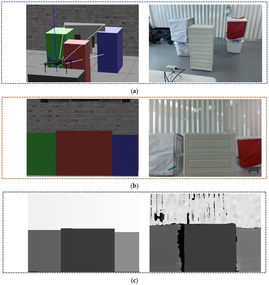
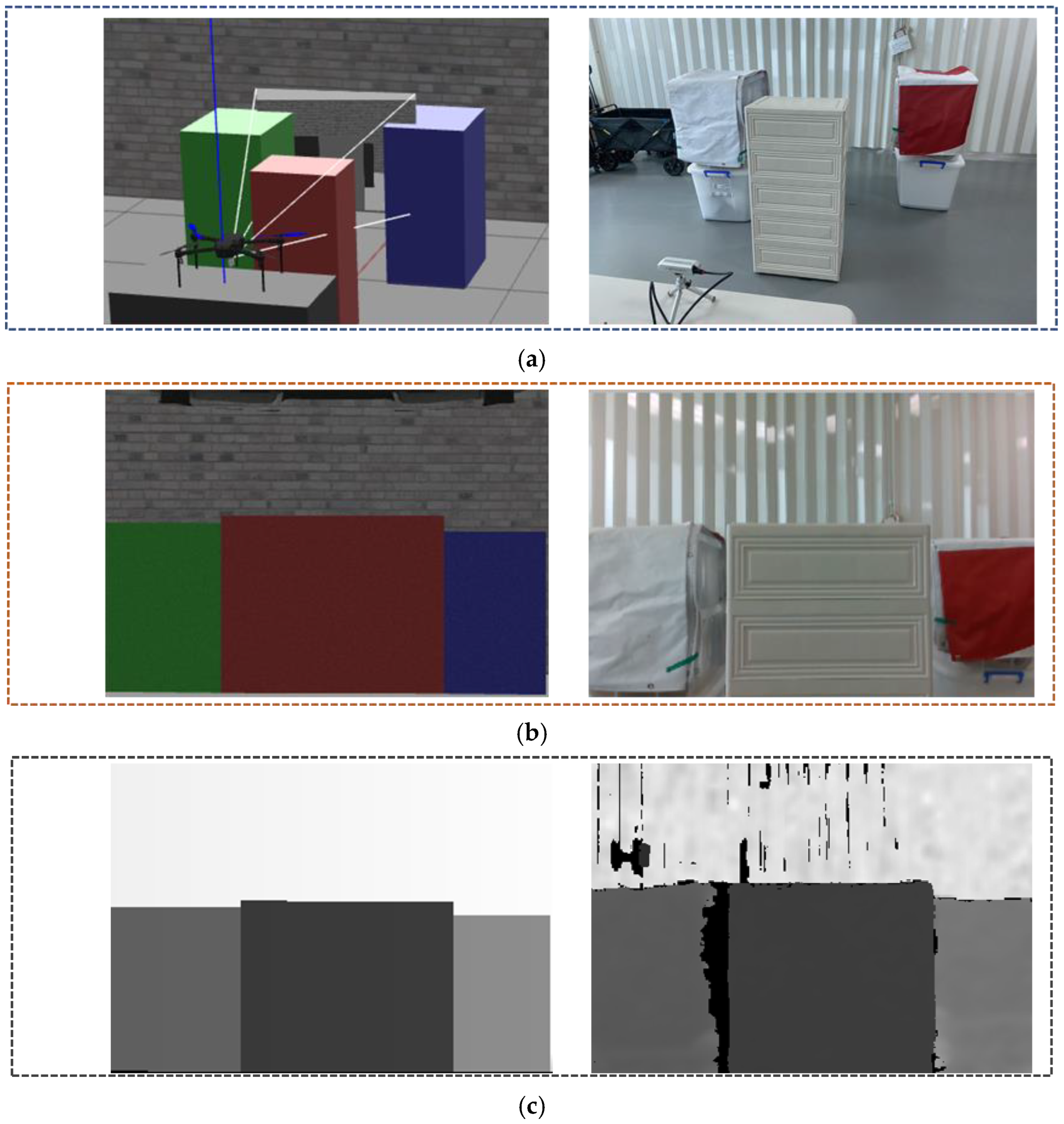
The experimental setup is illustrated in Figure 10. Three fixed obstacles were positioned in front of the camera at distances of 1.0 m, 1.5 m, and 2.0 m, respectively. Both the simulated and physical environments were configured to maintain consistent viewing angles, lighting conditions, and spatial arrangements to ensure data comparability.
Figure 10.
Comparison of simulated and physical test scenarios: (a) Experimental layout, with obstacle distances arranged from left to right at 1.5 m, 1.0 m, and 2.0 m, respectively; (b) First-person RGB images captured by the simulated and physical cameras under identical scene conditions; (c) First-person depth images acquired by the simulated and physical cameras within the same environment.
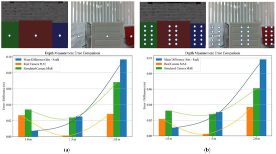
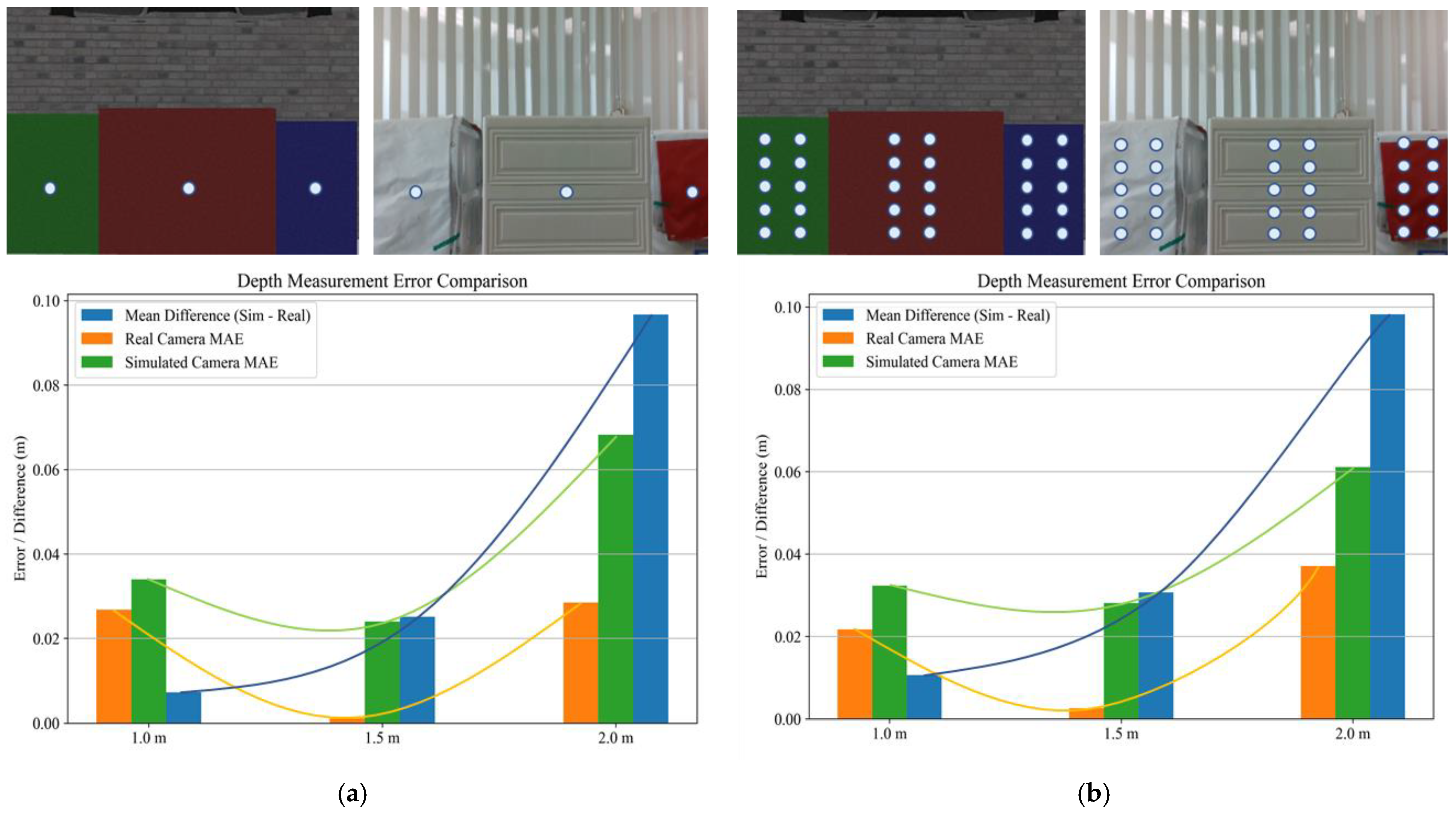
The experimental results are illustrated in Figure 11, with the corresponding statistical data summarized in Table 5 and Table 6.
Figure 11.
Depth measurement comparison between simulated and physical cameras: (a) Single-pixel evaluation, the simulated camera exhibits systematic overestimation with stable output, whereas the physical camera demonstrates greater variability due to environmental influences; (b) Multi-point sampling evaluation; both systems display consistent trends in error variation with respect to distance, while the deviation of the simulated camera becomes increasingly pronounced as distance increases.
Table 5.
Statistical results of single-pixel depth measurements at different distances using real and simulated cameras.
Table 6.
Statistical results of multi-point depth measurements at different distances using real and simulated cameras.
In the single-pixel evaluation, the simulated camera exhibited a systematic overestimation in depth output, with mean absolute errors ranging from 3.40 to 6.82 cm. Notably, the standard deviation remained below 0.12 cm, indicating a high degree of output stability. In contrast, the physical camera’s measurement error fell within the manufacturer’s specified accuracy range (±2–4 cm), with standard deviations between 0.2 and 1.4 cm, reflecting greater variability due to lighting conditions and surface material properties.
Both systems demonstrated optimal performance at a distance of 1.5 m, where the physical camera achieved a minimal error of only 0.73 cm.
In the multi-point sampling experiment, the results were consistent with those obtained from the single-pixel analysis. The simulated camera continued to exhibit systematic overestimation while maintaining low measurement noise. The physical camera achieved its highest accuracy at 1.5 m, with a mean error of 1.10 cm and an RMSE of 1.21 cm.
As the distance increased, the discrepancy between the simulated and physical measurements widened, with the mean difference expanding from 0.7 cm at 1.0 m to 9.7 cm at 2.0 m. This phenomenon is primarily attributable to the simplified modeling of illumination, surface reflection, and depth return mechanisms within the Gazebo simulation environment. These findings indicate that although the simulated system can provide consistent and low-noise depth data, calibration against physical measurements remains necessary to ensure practical reliability.
4.2. SLAM Localization Error Using Simulated Ground-Truth Pose Analysis
To evaluate the localization accuracy of the SLAM system, the estimated positions were compared with the simulated ground-truth pose provided by the Gazebo/ArduPilot SITL environment. Experiments were conducted in three obstacle-density scenarios—low, medium, and high—each comprising five traversal missions and five return missions.
Because the SLAM map is constructed in a relative coordinate frame, its initial origin and orientation do not coincide with those of the GPS reference frame. Therefore, prior to error computation, coordinate alignment and rotational transformation were performed to ensure that both trajectories were evaluated within a common reference framework.
To compensate for discrepancies between the SLAM and GPS coordinate systems, four alignment strategies were applied prior to error computation:
- Original: No alignment was performed; the two trajectories were compared directly.
- Rotated: A fixed angular correction was applied to adjust the overall orientation.
- Best angle: An optimal rotation angle within the range of 0–180° was determined by minimizing the RMSE.
- Initial angle: Alignment was conducted based on the initial directional vector, simulating a practical real-time application scenario.
To evaluate localization accuracy, three commonly adopted error metrics were employed: RMSE, Mean Error, and Maximum Error. Their computational formulations and interpretations are described as follows.
First, RMSE was utilized to quantify the overall deviation between the SLAM-estimated and GPS-referenced coordinates, thereby reflecting the global stability of the localization system. The definition is given in Equation (15):
where denotes the total number of data points, and and represent the SLAM and GPS coordinates of the -th data sample, respectively.
The Mean Error represents the average Euclidean distance between corresponding coordinate pairs and is used to characterize the overall positional deviation trend. Its formulation is provided in Equation (16):
The Maximum Error is employed to identify the largest deviation among all sampled points, thereby capturing potential extreme discrepancies that may occur in specific trajectory segments during SLAM operation. Its formulation is presented in Equation (17):
In this study, five traversal missions and five return missions were conducted in each obstacle-density environment to compare localization errors between SLAM and GPS. The corresponding statistical results are summarized in Table 7.
Table 7.
Comparison of traversal and return missions in three density maps.
- Medium-density obstacle scenario
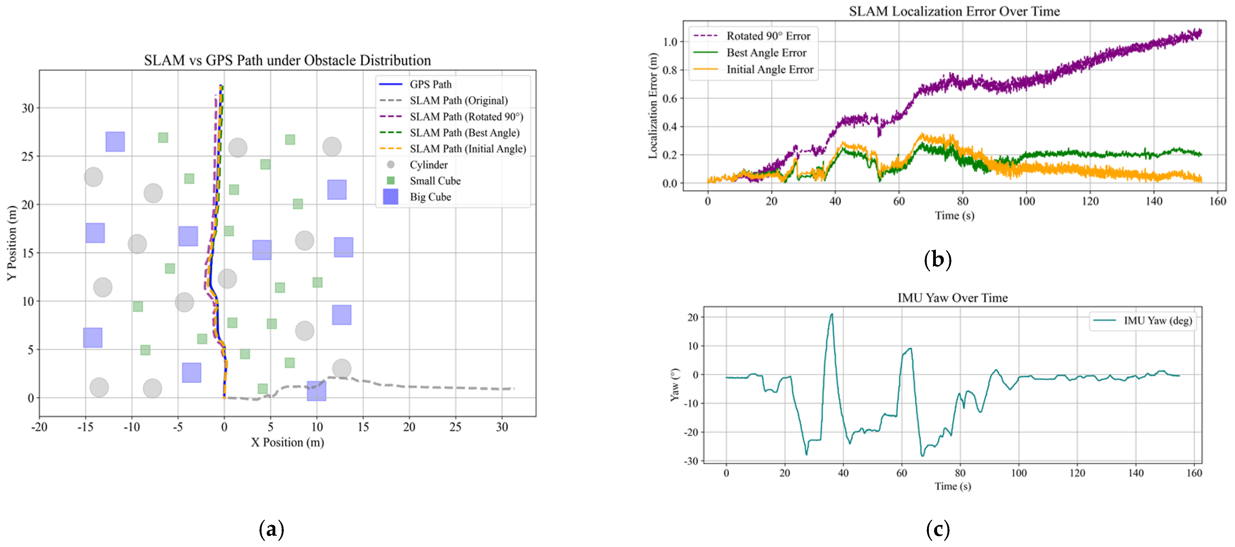
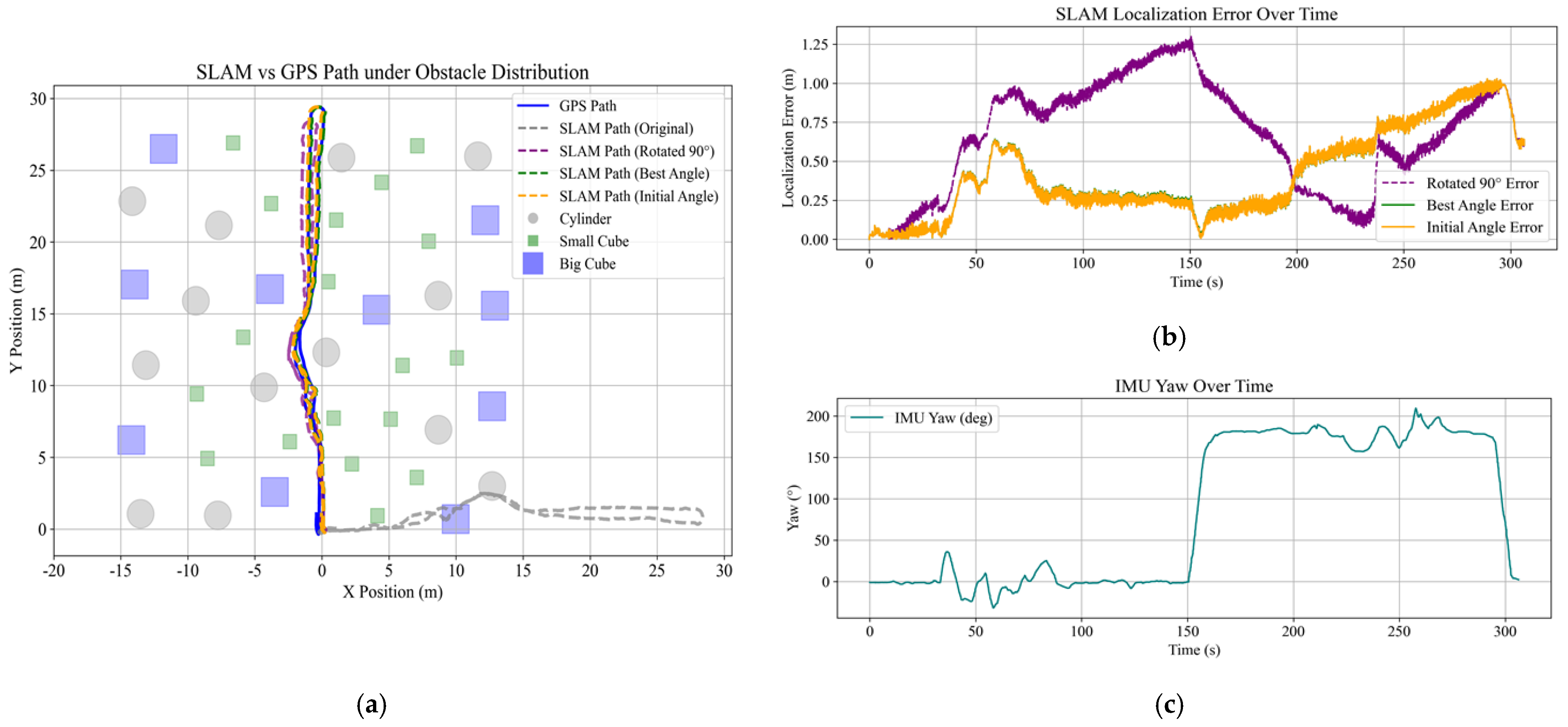
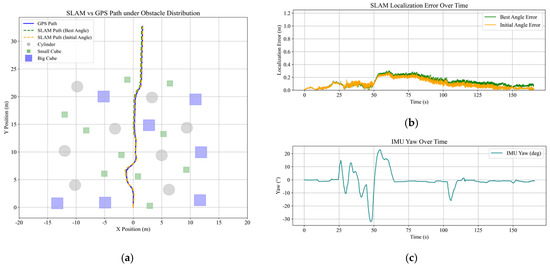
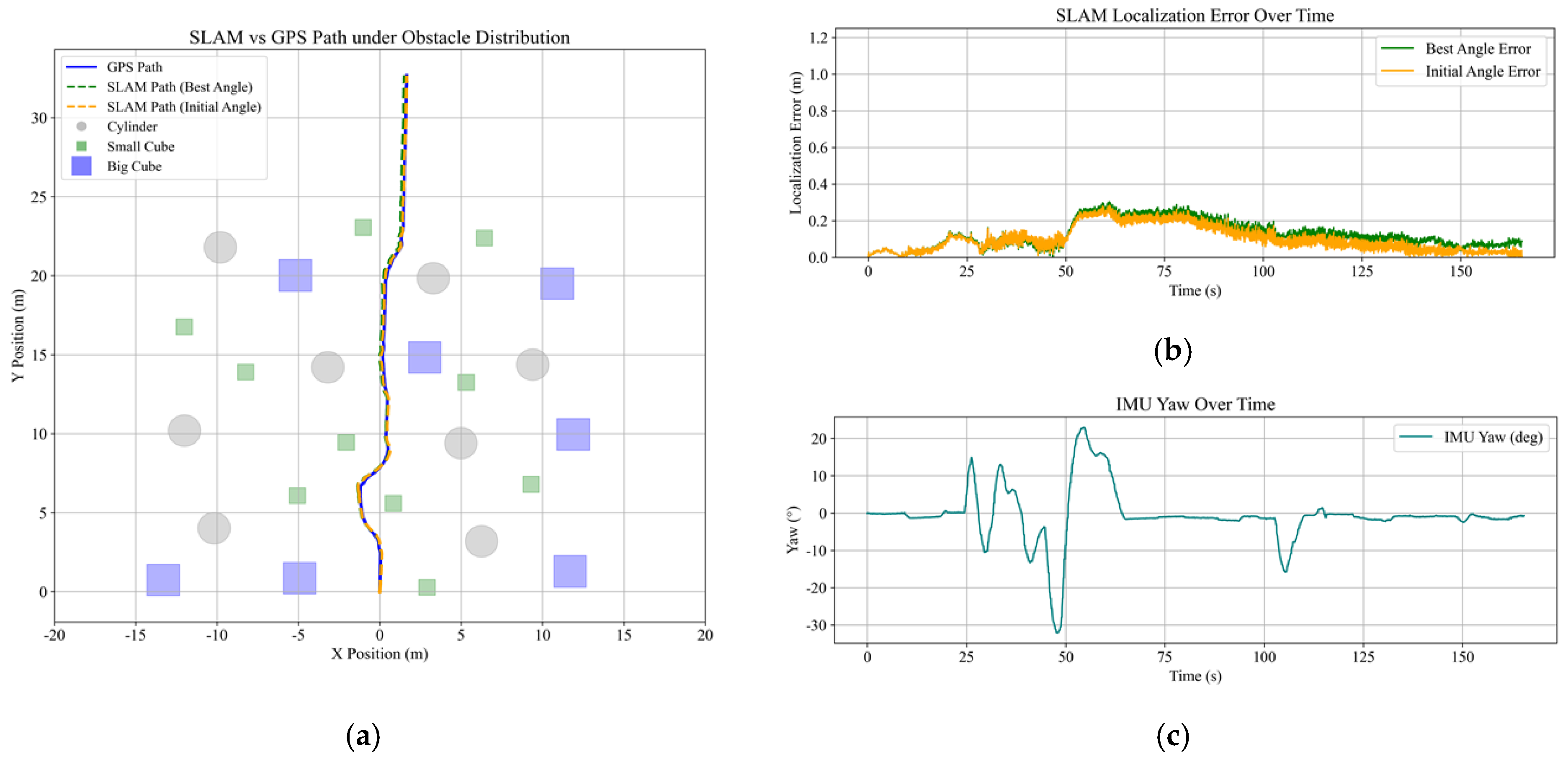
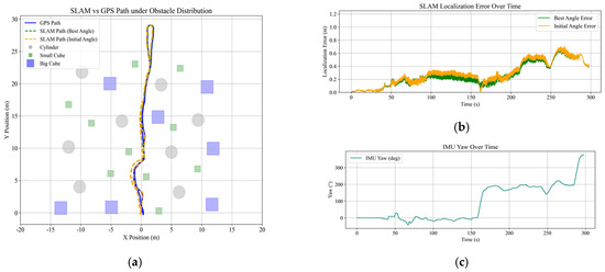
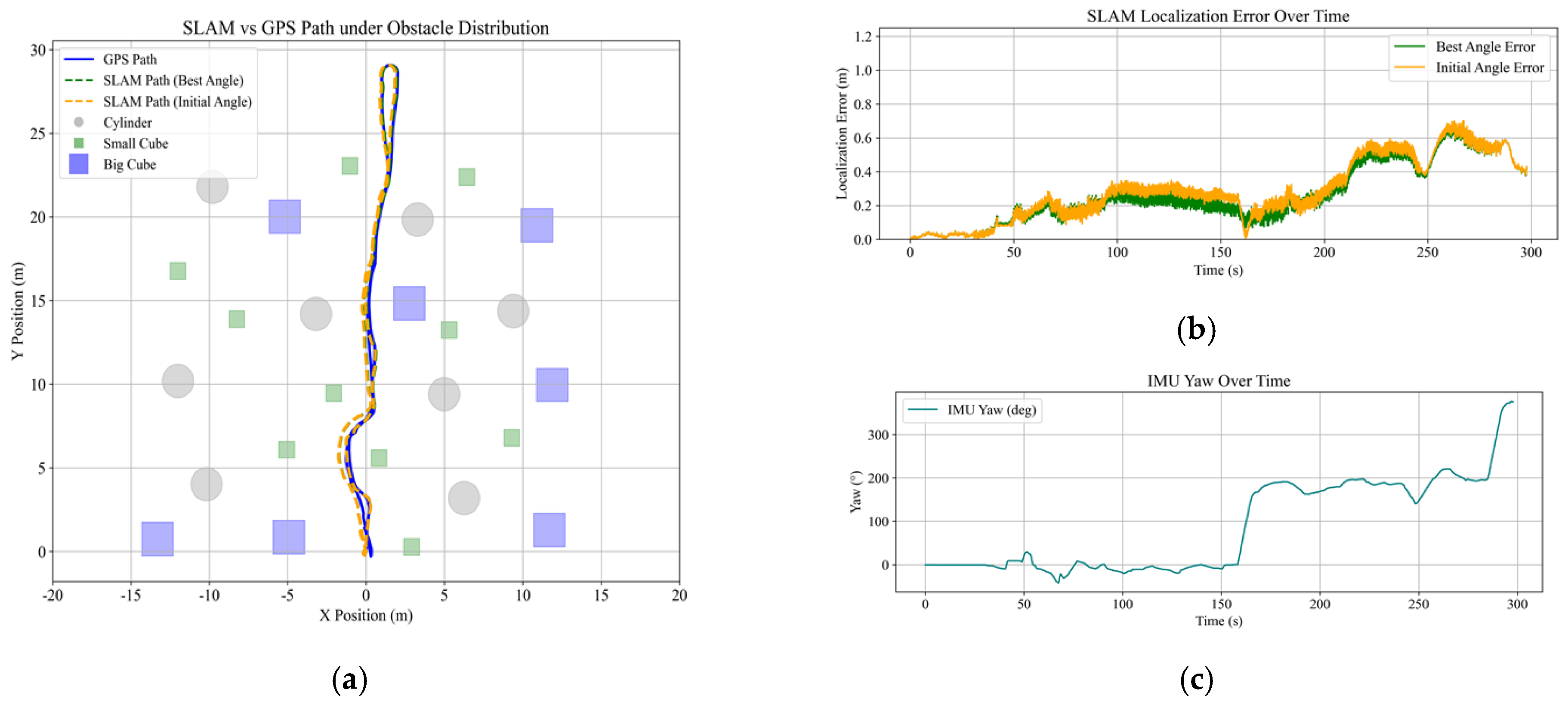
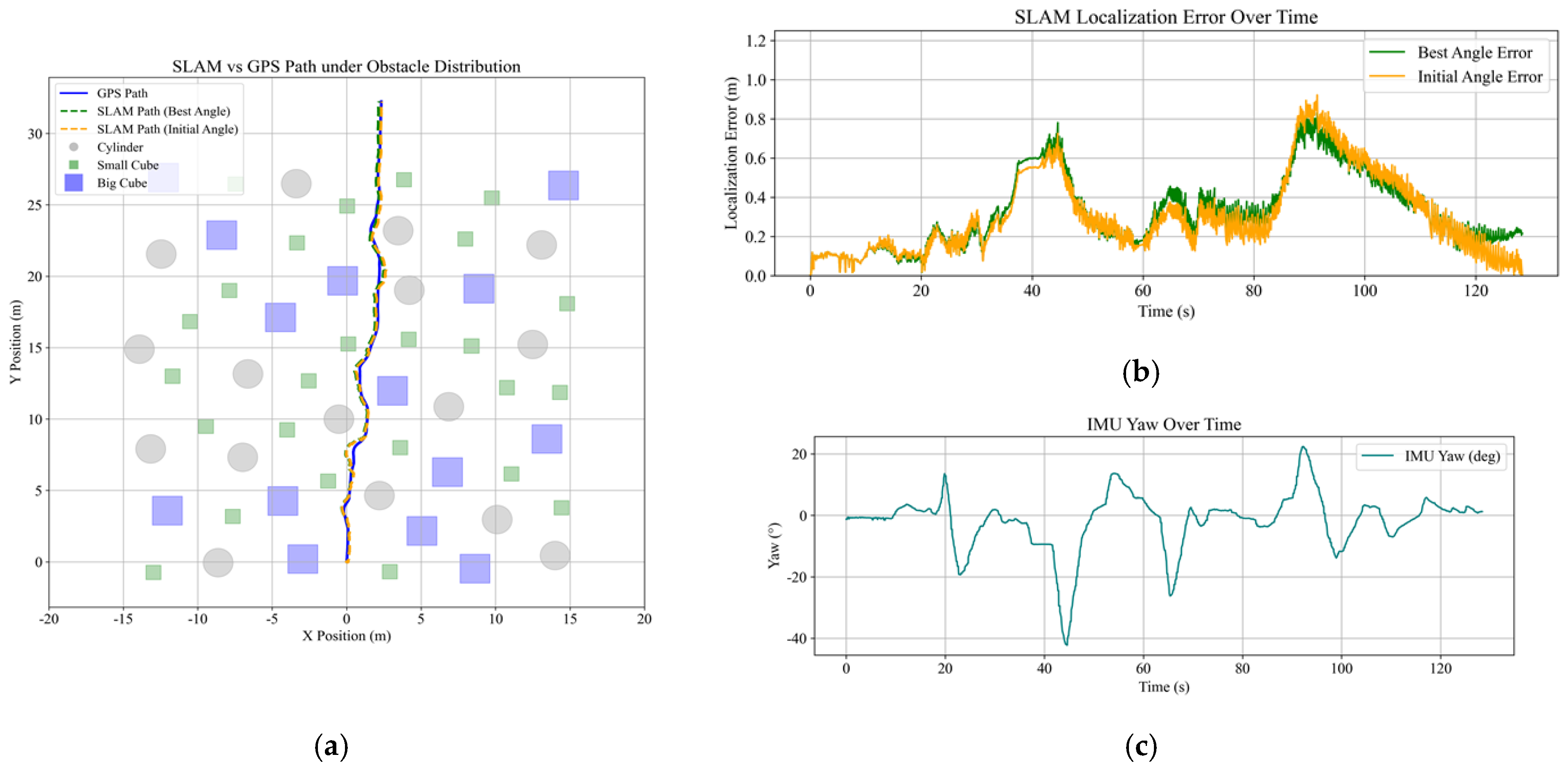
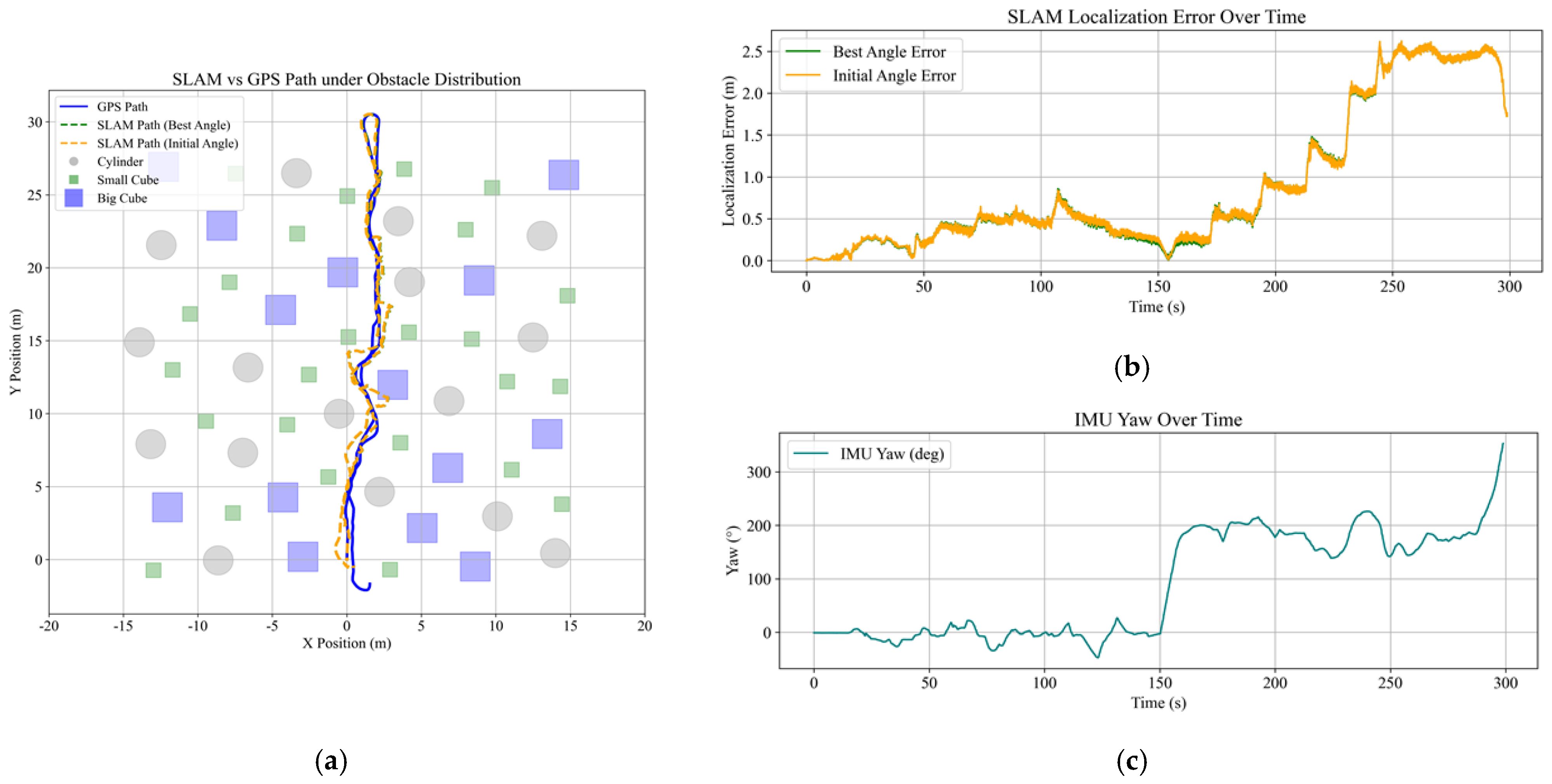
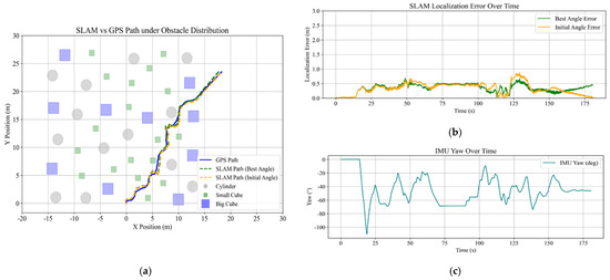
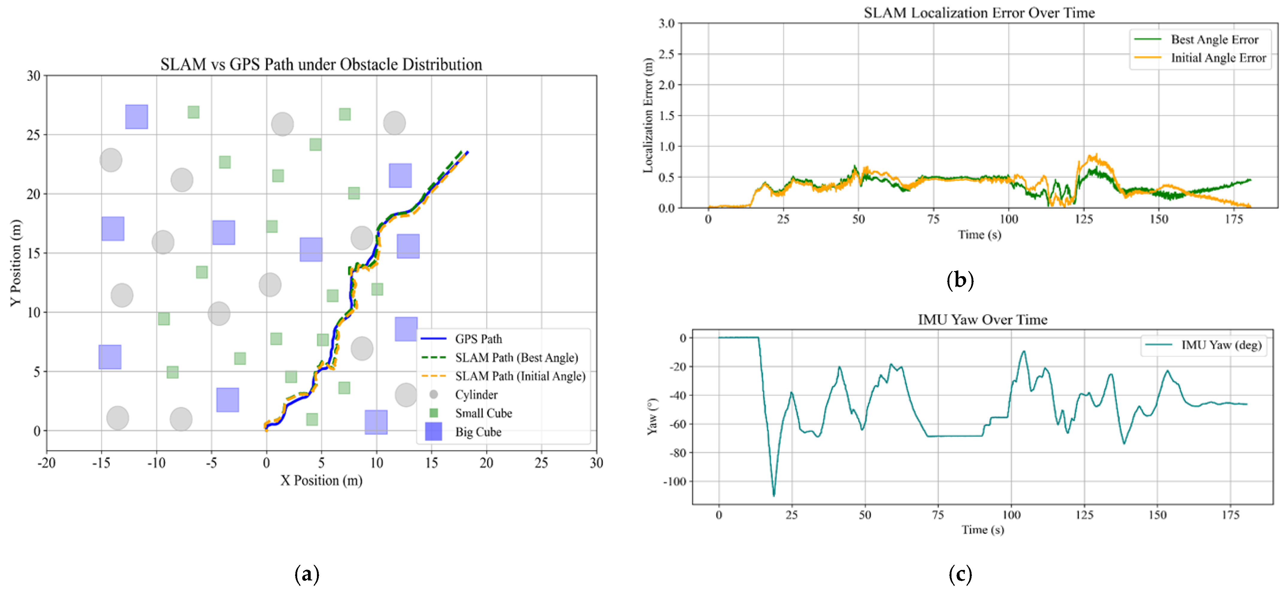
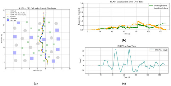
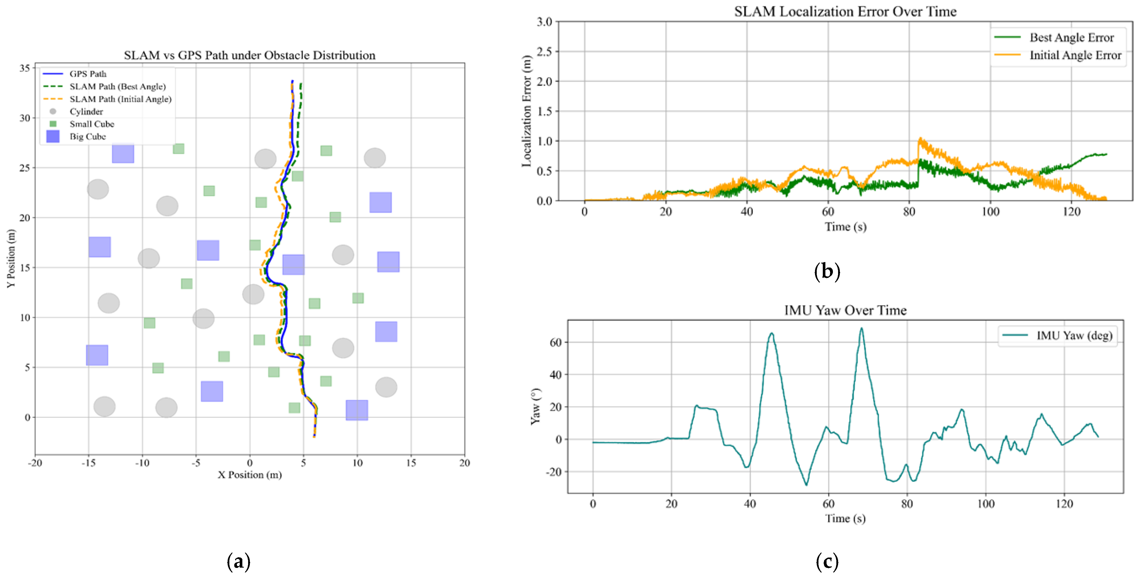
As illustrated in Figure 12a and Figure 13b, under the unaligned condition, the RMSE values for the traversal and return missions were 25.93 m and 23.48 m, respectively, indicating substantial discrepancies between the original coordinate frames. Following alignment, the errors were markedly reduced. Among the evaluated strategies, the Best Angle method achieved the lowest RMSE, reducing it to 0.183 m for traversal and 0.473 m for return missions. The Initial Angle method yielded RMSE values of 0.197 m and 0.474 m, respectively, demonstrating performance comparable to that of the optimal rotation approach.
Figure 12.
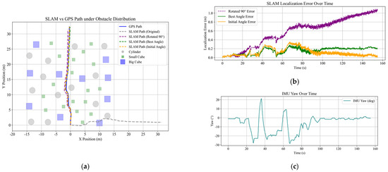
Localization comparison between SLAM and GPS during autonomous traversal in the medium-density scenario: (a) Comparison of SLAM and GPS trajectories, with obstacle distribution illustrated; (b) Localization error curves under different coordinate alignment strategies; (c) Temporal variation in the IMU yaw angle.
Figure 13.
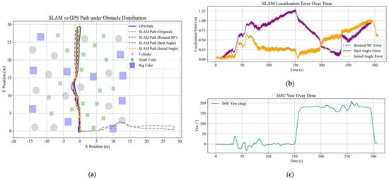
Localization comparison between SLAM and GPS during autonomous return in the medium-density scenario: (a) Comparison of SLAM and GPS trajectories, with obstacle distribution illustrated; (b) Localization error curves under different coordinate alignment strategies; (c) Temporal variation in the IMU yaw angle.
It should be noted that the Best Angle method requires access to the complete trajectory to search for the optimal rotation angle and is therefore applicable only to offline analysis. In contrast, the Initial Angle method estimates the coordinate misalignment based on the initial heading vector and vehicle orientation at the beginning of the mission, and applies the corresponding correction without relying on GPS throughout the entire trajectory. As a result, it exhibits greater potential for real-time deployment.
The error performance of the Initial Angle approach is nearly identical to that of the optimal rotation method, indicating that it can maintain stability and accuracy during return missions as well. This demonstrates its practical feasibility. Accordingly, subsequent experiments and result analyses focus primarily on comparisons between the Best Angle and Initial Angle strategies.
A further examination of the localization error trends during traversal and return missions indicates that the observed differences are primarily associated with flight maneuver characteristics.
In the traversal mission, as shown in Figure 12b, the discrepancy between SLAM and GPS remains generally stable, demonstrating satisfactory temporal continuity and error convergence of the system. However, a pronounced increase in the error curve is observed between approximately 37 and 100 s. By correlating this interval with the yaw angle variation depicted in Figure 12c, it is evident that the UAV executed multiple turning maneuvers for obstacle avoidance during this period. Frequent directional changes induced abrupt shifts in the camera’s field of view, thereby destabilizing visual feature matching and temporarily increasing SLAM trajectory estimation error.
In the return mission, as illustrated in Figure 13b, the error curve remains relatively stable during the initial phase of the task but exhibits a pronounced increase after approximately 150 s, corresponding to the UAV’s execution of an approximately 180° turning maneuver. This large-angle rotation introduced a directional deviation in SLAM pose estimation, resulting in a temporary degradation of localization accuracy. The yaw angle variation shown in Figure 13c further corroborates this turning behavior.
Nevertheless, as the UAV gradually approached the initial position and reoriented its heading, the loop closure mechanism successfully matched historical visual features, thereby correcting the accumulated localization error. Consequently, even within the medium-density environment, the system was able to effectively constrain localization error within ±0.5 m through the combined effects of loop closure detection and initial orientation alignment, demonstrating both stability and practical applicability.
- Low-density obstacle scenario
In the low-density obstacle environment, five traversal and five return missions were likewise conducted to compare SLAM and GPS trajectories, with the results presented in Figure 14 and Figure 15. Overall, the localization error curves remain stable with minimal fluctuation, indicating that the SLAM system maintains strong temporal continuity and error stability in open environments.
Figure 14.
Localization comparison between SLAM and GPS during autonomous traversal in the low-density scenario: (a) Comparison of SLAM and GPS trajectories, with obstacle distribution illustrated; (b) Localization error curves under different coordinate alignment strategies; (c) Temporal variation in the IMU yaw angle.
Figure 15.
Localization comparison between SLAM and GPS during autonomous return in the low-density scenario: (a) Comparison of SLAM and GPS trajectories, with obstacle distribution illustrated; (b) Localization error curves under different coordinate alignment strategies; (c) Temporal variation in the IMU yaw angle.
With respect to alignment strategies, the Best Angle method again achieved the lowest error, yielding RMSE values of 0.193 m for traversal and 0.281 m for return missions. The Initial Angle method produced comparable results of 0.195 m and 0.295 m, respectively.
The limited increases observed in certain segments of the error curves correspond to UAV turning maneuvers, as illustrated in Figure 14b,c and Figure 15b,c, though their magnitudes are substantially lower than those observed in the medium-density scenario. In comparison, the maximum localization errors for traversal and return missions decreased by approximately 0.07 m and 0.32 m, respectively. These findings further substantiate the influence of environmental occlusion on the stability of visual SLAM algorithms.
- High-density obstacle scenario
In the high-density obstacle environment, comparisons between SLAM and GPS trajectories for traversal and return missions are presented in Figure 16 and Figure 17. Using the Best Angle strategy, the RMSE values were 0.347 m for traversal and 1.022 m for return missions. The Initial Angle method yielded RMSE values of 0.420 m and 1.084 m, respectively. These results indicate that even under the optimal alignment strategy, the return mission error remains substantially higher than that of traversal, with a difference of approximately 0.67 m.
Figure 16.
Localization comparison between SLAM and GPS during autonomous traversal in the high-density scenario: (a) Comparison of SLAM and GPS trajectories, with obstacle distribution illustrated; (b) Localization error curves under different coordinate alignment strategies; (c) Temporal variation in the IMU yaw angle.
Figure 17.
Localization comparison between SLAM and GPS during autonomous return in the high-density scenario: (a) Comparison of SLAM and GPS trajectories, with obstacle distribution illustrated; (b) Localization error curves under different coordinate alignment strategies; (c) Temporal variation in the IMU yaw angle.
The error curves exhibit frequent fluctuations, including multiple segments of abrupt error escalation, corresponding to repeated turning and obstacle avoidance maneuvers within confined spaces, as shown in Figure 16b,c and Figure 17b,c. This phenomenon reflects the increased likelihood of visual feature loss or mismatching in complex terrains, leading to transient drift in SLAM estimation. Notably, during the return phase, the time required for the error to recover to a stable level is significantly prolonged, indicating that the corrective effectiveness of loop closure detection is constrained under conditions of severe environmental occlusion.
Across the three obstacle-density scenarios, the UAV successfully completed both traversal and return missions in all cases. Overall, localization error during traversal missions was consistently lower than that observed during return missions. The former benefited from a more uniform path direction and sustained visual continuity, whereas the latter involved frequent turning and large-angle maneuvers, leading to feature loss and increased estimation uncertainty.
Environmental density was also found to exert a significant influence on localization accuracy. In the high-density scenario, the maximum RMSE reached 1.084 m. The localization errors were evaluated with respect to the simulated ground-truth pose. A direct comparison with real GNSS performance is not considered a fair comparison in this study.
4.3. Localization Error Analysis Under Varying Exploration Orientations and Starting Configurations
To evaluate the robustness of the SLAM system under different initial conditions, two experimental scenarios were designed. The first scenario fixed the starting position while varying the exploration direction; the second maintained a constant exploration direction while altering the starting position. In each of the three obstacle-density environments, five traversal and five return missions were conducted, with performance assessed using RMSE, Mean Error, and Maximum Error.
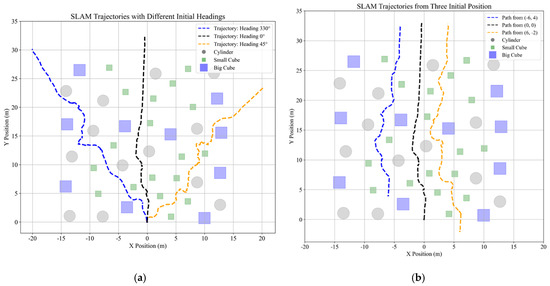
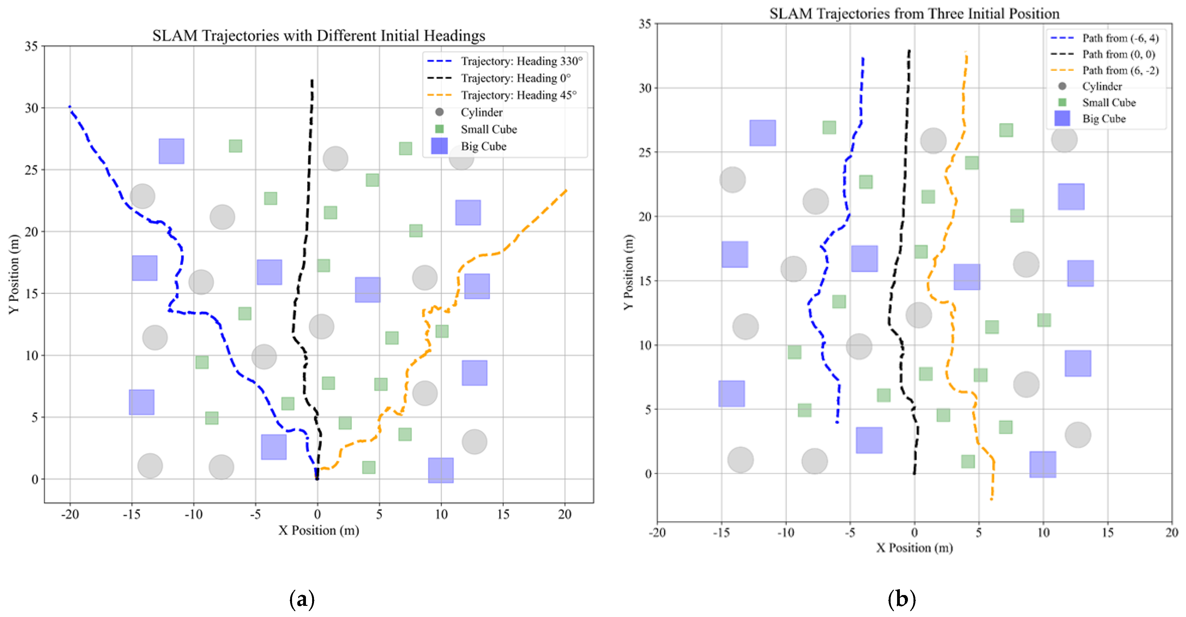
For each exploration orientation and starting configuration, multiple traversal missions were performed to compare localization discrepancies between SLAM and GPS. The statistical results are summarized in Table 8, and representative trajectories under different initial conditions are illustrated in Figure 18.
Table 8.
Comparison of different initial conditions in the medium-density map.
Figure 18.
Comparison of SLAM and GPS trajectories under different initial conditions in the medium-density scenario: (a) Different exploration orientations; (b) Different starting position configurations.
- Exploration Direction Variation (Fixed Start, Varying Direction)
In the medium-density environment, when the starting position was fixed at the center of the map and traversal missions were executed along different exploration directions, the error magnitude exhibited moderate variation depending on the selected heading. For example, along the 330° northwest and 45° northeast directions, the RMSE after initial orientation alignment was 0.438 m and 0.373 m, respectively, representing an increase of approximately 0.15–0.30 m compared with the northbound mission (0.197 m).
The corresponding error curves and yaw angle variations are presented in Figure 19. When the exploration direction deviated from the forward-facing orientation, the UAV was required to perform more frequent turning and obstacle avoidance maneuvers, resulting in amplified heading fluctuations and consequently elevating the risk of cumulative SLAM estimation error.
Figure 19.
Localization comparison between SLAM and GPS during the 45° northeast traversal mission in the medium-density scenario: (a) Comparison of SLAM and GPS trajectories, with obstacle distribution illustrated; (b) Localization error curves under different coordinate alignment strategies; (c) Temporal variation in the IMU yaw angle.
These findings indicate that although directional variation influences localization accuracy to a certain extent, the system is nevertheless capable of maintaining stable positioning performance.
- Starting Position Variation (Fixed Direction, Varying Start)
When the exploration direction was fixed at due north (0°), but the starting position was set at three different locations (0, 0), (6, −2), and (−6, 4), the corresponding RMSE values were 0.197 m, 0.349 m, and 0.249 m, respectively. Although variations in the starting position introduced differences in the early-stage trajectory, the final localization error in all cases remained within 0.40 m.
The associated error curves and yaw angle variations are presented in Figure 20. Changes in the starting position primarily affected the frequency of obstacle avoidance maneuvers during the initial navigation phase; however, no substantial difference was observed in overall SLAM accuracy. These results demonstrate a high degree of tolerance to initial position variations within the proposed system.
Figure 20.
Localization comparison between SLAM and GPS during the traversal mission with initial position (6, −2) in the medium-density scenario: (a) Comparison of SLAM and GPS trajectories, with obstacle distribution illustrated; (b) Localization error curves under different coordinate alignment strategies; (c) Temporal variation in the IMU yaw angle.
The overall results indicate that variations in exploration direction, due to differences in obstacle distribution, may increase the frequency of turning maneuvers and attitude adjustments, thereby leading to a moderate rise in localization error. In contrast, changes in the starting position primarily affect the initial path planning phase and exert only limited influence on the final localization accuracy.
In general, even under conditions where both exploration direction and starting position are altered, the SLAM error remains consistently within ±0.5 m. These findings validate the adaptability and operational flexibility of the proposed system.
4.4. Navigation with Dynamic Obstacles
To evaluate the system’s real-time responsiveness and obstacle avoidance capability in dynamic environments, additional obstacles were manually introduced along the predefined navigation trajectory within the low-density map, simulating unexpected disturbances that may occur in forested scenarios. During the experiment, RTAB-Map continuously updated the map representation, while move_base (DWA) performed real-time local replanning, enabling the UAV to successfully circumvent the obstacles and complete the mission.
The evaluation focused primarily on obstacle avoidance success and path deviation characteristics, with qualitative validation provided through visualization results in RViz and Gazebo.
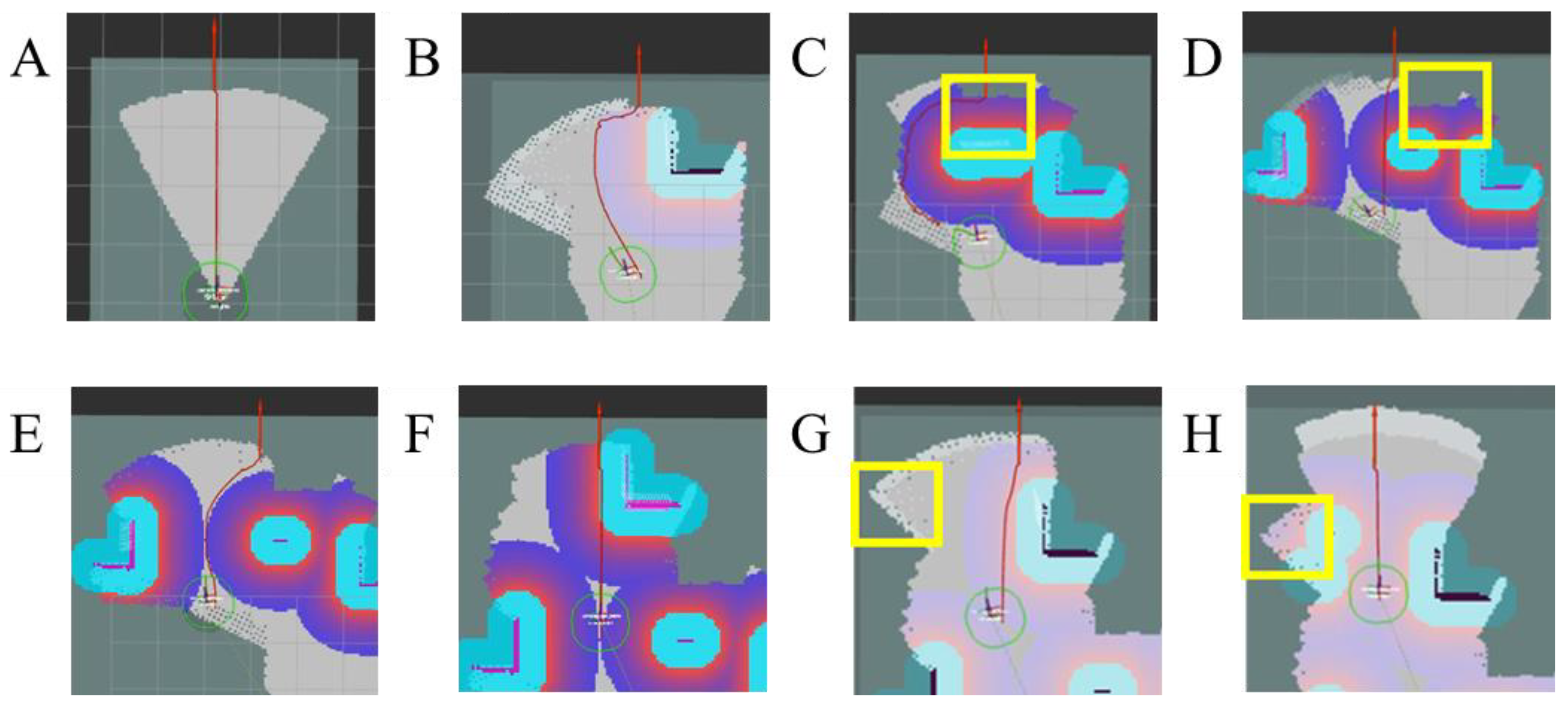
Figure 21 and Figure 22 illustrate the UAV navigation trajectories during traversal and return missions, respectively, when dynamic obstacles were introduced. The following observations can be made:
Figure 21.
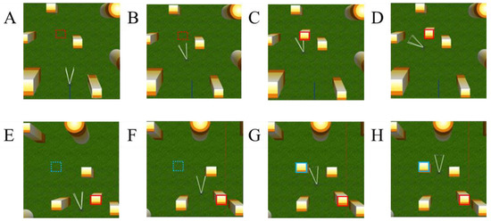
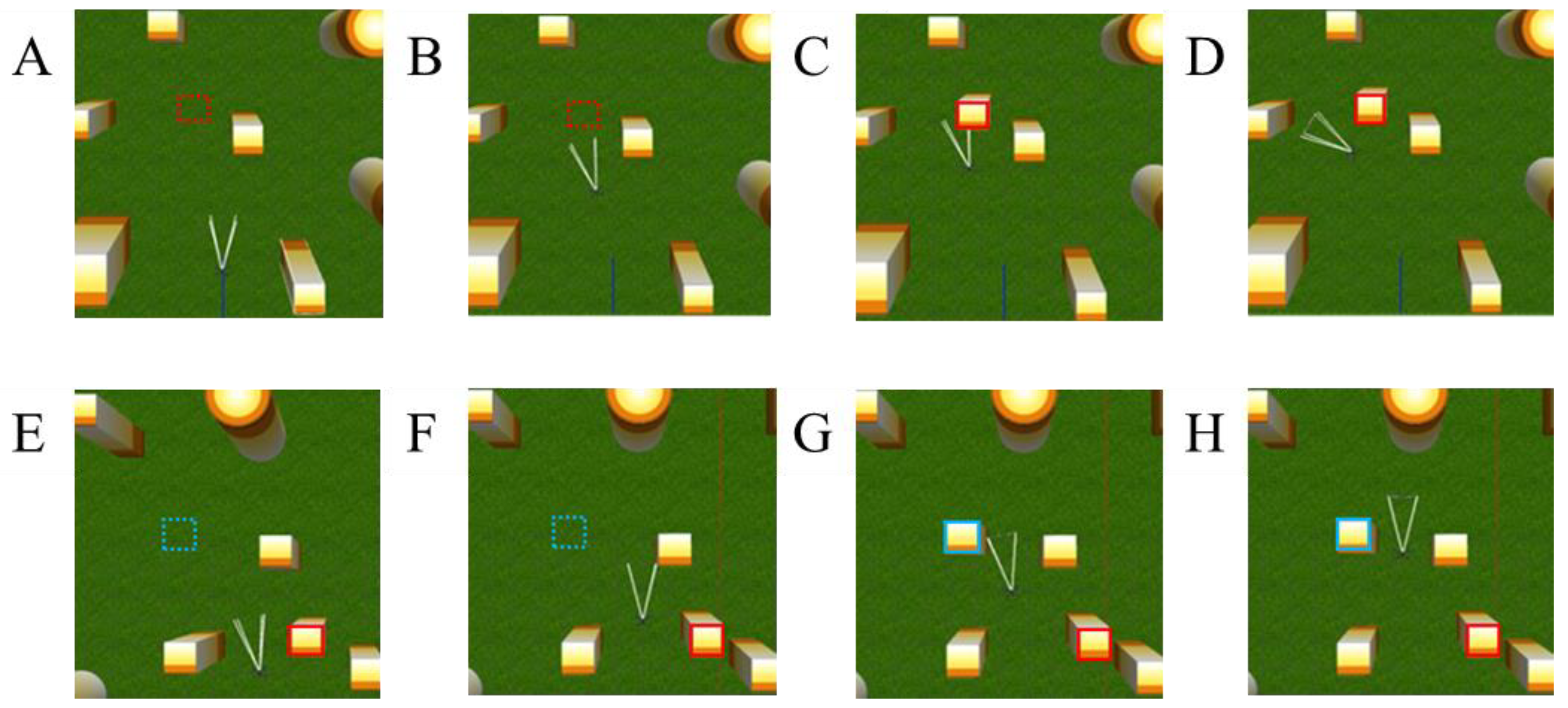
UAV encounter with a dynamic obstacle in the Gazebo simulation environment: (A) initial navigation state before obstacle insertion; (B,C) dynamic obstacle insertion along the UAV trajectory (red dashed box/red solid box); (D) UAV heading adjustment and local avoidance maneuver; (E,F) additional dynamic obstacle insertion during navigation (blue dashed box/blue solid box); (G,H) successful obstacle avoidance and continuation toward the target direction.
Figure 22.
Map update and local replanning process visualized in RViz during dynamic obstacle avoidance: (A,B) normal navigation before obstacle detection; (C,D) obstacle detection and local costmap update (yellow box); (E,F) local trajectory replanning and obstacle avoidance; (G,H) continued navigation with detection of a second dynamic obstacle (yellow box), triggering an additional local replanning process. The colored regions represent local costmap updates generated from depth sensing, while the red trajectory line indicates the UAV navigation path. The colored regions represent local costmap updates generated from depth sensing, while the red trajectory line indicates the UAV navigation path.
- Dynamic sensing and replanning: Once an obstacle entered the sensing range, the depth camera output promptly updated the local costmap, while the SLAM module simultaneously incorporated the newly detected obstacle into the map representation. The navigation module subsequently triggered real-time path replanning.
- Obstacle avoidance behavior: The UAV adjusted its heading prior to direct interception with the obstacle, generating a detour trajectory. After clearing the obstacle, it resumed its original navigation direction.
- Success rate: Across five experimental trials, the UAV successfully avoided the introduced obstacles and completed both exploration and return missions, demonstrating the reliability of the proposed system.
The system was evaluated in a Gazebo simulation environment, where manually introduced sudden dynamic obstacles were placed approximately 1–2 m in front of the UAV during navigation. The experimental results demonstrated that the system could update the SLAM map and costmap in real time and perform local path replanning through the DWA module, thereby effectively avoiding collisions while continuously executing the navigation task.
It should be noted that this experiment is a qualitative demonstration of dynamic-obstacle response. Quantitative metrics such as replanning latency, minimum obstacle clearance, path-length increase, and mission completion time were not systematically evaluated. In addition, quantitative success rate and mission completion metrics were not systematically evaluated. Therefore, the results should be interpreted as preliminary evidence of local replanning capability.
5. Conclusions
This study presents a lightweight UAV navigation framework using a single depth camera and demonstrates its performance through simulation-based experiments.
It should be emphasized that the current evaluation is primarily simulation-based. The results should not be interpreted as real-world deployment readiness.
Several limitations remain:
- (1)
- Simplified environments;
- (2)
- Planar navigation;
- (3)
- No baseline comparison;
- (4)
- Qualitative dynamic obstacle evaluation.
Therefore, the results represent feasibility validation only.
Future work will include real UAV experiments, realistic environments, 3D navigation, and baseline comparison.
Author Contributions
Conceptualization, Y.-T.W. and Y.-C.H.; methodology, Y.-T.W.; software, Y.-T.W.; validation, Y.-T.W.; formal analysis, Y.-T.W.; investigation, Y.-T.W.; resources, Y.-T.W. and Y.-C.H.; data curation, Y.-T.W.; writing—original draft preparation, Y.-T.W. and Y.-C.H.; writing—review and editing, Y.-T.W. and Y.-C.H.; visualization, Y.-T.W.; supervision, Y.-C.H.; project administration, Y.-T.W. and Y.-C.H.; funding acquisition, Y.-C.H. All authors have read and agreed to the published version of the manuscript.
Funding
This research was funded by the National Science and Technology Council in part with grant number 114-2218-E-005-004.
Data Availability Statement
The data presented in this study are available upon request from the author.
Acknowledgments
The authors gratefully acknowledge the National Science and Technology Council for partial financial support.
Conflicts of Interest
The authors declare no conflicts of interest. The funders had no role in the design of the study; in the collection, analyses, or interpretation of data; in the writing of the manuscript; or in the decision to publish the results.
Abbreviations
The following abbreviations are used in this manuscript:
| UAV | Unmanned Aerial Vehicle |
| GPS | Global Positioning System |
| SLAM | Simultaneous Localization and Mapping |
| RTAB-Map | Real-Time Appearance-Based Mapping |
| VIO | Visual–Inertial Odometry |
| IMU | Inertial Measurement Unit |
| SITL | Software-In-The-Loop |
| FOV | Field of View |
| DWA | Dynamic Window Approach |
| STM | Short-Term Memory |
| VO | Visual Odometry |
| F2F | Frame-to-Frame |
| F2M | Frame-to-Map |
| WM | Working Memory |
| BoW | Bag-of-Words |
| LTM | Long-Term Memory |
| GCR | Ground Trunk Coverage Ratio |
| RMSE | Root Mean Square Error |
References
- Smith, R.C.; Cheeseman, P. On the Representation and Estimation of Spatial Uncertainty. Int. J. Robot. Res. 1986, 5, 56–68. [Google Scholar] [CrossRef] [Scilit]
- Grisetti, G.; Stachniss, C.; Burgard, W. Improved Techniques for Grid Mapping With Rao-Blackwellized Particle Filters. IEEE Trans. Robot. 2007, 23, 34–46. [Google Scholar] [CrossRef] [Scilit]
- Kohlbrecher, S.; von Stryk, O.; Meyer, J.; Klingauf, U. A Flexible and Scalable SLAM System with Full 3D Motion Estimation. In Proceedings of the 2011 IEEE International Symposium on Safety, Security, and Rescue Robotics, Kyoto, Japan, 1–5 November 2011; pp. 155–160. [Google Scholar] [CrossRef] [Scilit]
- Jeong, W.; Lee, C.; Lee, N.; Hong, S.; Kang, D.; An, D. Improving Sensor Adaptability and Functionality in Cartographer Simultaneous Localization and Mapping. Sensors 2025, 25, 1808. [Google Scholar] [CrossRef] [Scilit] [PubMed]
- Campos, C.; Elvira, R.; Rodríguez, J.J.G.; M. Montiel, J.M.; D. Tardós, J. ORB-SLAM3: An Accurate Open-Source Library for Visual, Visual–Inertial, and Multimap SLAM. IEEE Trans. Robot. 2021, 37, 1874–1890. [Google Scholar] [CrossRef] [Scilit]
- Labbé, M.; Michaud, F. RTAB-Map as an Open-Source Lidar and Visual Simultaneous Localization and Mapping Library for Large-Scale and Long-Term Online Operation. J. Field Robot. 2019, 36, 416–446. [Google Scholar] [CrossRef] [Scilit]
- Xiao, J.; Zhang, R.; Zhang, Y.; Feroskhan, M. Vision-Based Learning for Drones: A Survey. IEEE Trans. Neural Netw. Learn. Syst. 2025, 36, 15601–15621. [Google Scholar] [CrossRef] [Scilit] [PubMed]
- Xu, K.; Hao, Y.; Yuan, S.; Wang, C.; Xie, L. AirSLAM: An Efficient and Illumination-Robust Point-Line Visual SLAM System. IEEE Trans. Robot. 2025, 41, 1673–1692. [Google Scholar] [CrossRef] [Scilit]
- Forster, C.; Carlone, L.; Dellaert, F.; Scaramuzza, D. On-Manifold Preintegration for Real-Time Visual–Inertial Odometry. IEEE Trans. Robot. 2017, 33, 1–21. [Google Scholar] [CrossRef] [Scilit]
- Intel RealSense D400 Series Product Family. Available online: https://cdrdv2-public.intel.com/841984/Intel-RealSense-D400-Series-Datasheet.pdf (accessed on 28 June 2025).
- Intel RealSense Depth Camera. Available online: https://ardupilot.org/copter/docs/common-realsense-depth-camera.html (accessed on 29 June 2025).
- Xu, Z.; Zhan, X.; Chen, B.; Xiu, Y.; Yang, C.; Shimada, K. A Real-Time Dynamic Obstacle Tracking and Mapping System for UAV Navigation and Collision Avoidance with an RGB-D Camera. In Proceedings of the 2023 IEEE International Conference on Robotics and Automation (ICRA), London, UK, 29 May–2 June 2023; pp. 10645–10651. [Google Scholar] [CrossRef] [Scilit]
- Phan, H.-A.; Nguyen, P.V.; Thi Khuat, T.H.; Dang Van, H.; Quoc Tran, D.H.; Dang, B.L.; Bui, T.T.; Thi Thanh, V.N.; Duc, T.C. A Sensor Fusion Approach for Improving Implementation Speed and Accuracy of RTAB-Map Algorithm Based Indoor 3D Mapping. In Proceedings of the 2023 20th International Joint Conference on Computer Science and Software Engineering (JCSSE), Phitsanulok, Thailand, 28 June–1 July 2023; pp. 219–224. [Google Scholar] [CrossRef] [Scilit]
- Yamauchi, B. A Frontier-Based Approach for Autonomous Exploration. In Proceedings of the Proceedings 1997 IEEE International Symposium on Computational Intelligence in Robotics and Automation, CIRA’97. “Towards New Computational Principles for Robotics and Automation”, Monterey, CA, USA, 10–11 July 1997; pp. 146–151. [Google Scholar] [CrossRef] [Scilit]
- Ribeiro, A.; Basiri, M. Efficient 3D Exploration with Distributed Multi-UAV Teams: Integrating Frontier-Based and Next-Best-View Planning. Drones 2024, 8, 630. [Google Scholar] [CrossRef] [Scilit]
- Zhang, X.; Wang, J.; Wang, S.; Wang, M.; Wang, T.; Feng, Z.; Zhu, S.; Zheng, E. FAEM: Fast Autonomous Exploration for UAV in Large-Scale Unknown Environments Using LiDAR-Based Mapping. Drones 2025, 9, 423. [Google Scholar] [CrossRef] [Scilit]
- Github Intelligent-Quads/Iq_sim. Available online: https://github.com/Intelligent-Quads/iq_sim (accessed on 30 June 2025).
- Github Nilseuropa/Realsense_ros_gazebo. Available online: https://github.com/nilseuropa/realsense_ros_gazebo (accessed on 2 July 2025).
- Github Ros-Perception/Depthimage_to_laserscan. Available online: https://github.com/ros-perception/depthimage_to_laserscan (accessed on 4 July 2025).
- Move_base—ROS Wiki. Available online: https://wiki.ros.org/move_base (accessed on 6 July 2025).
- Labbé, M.; Michaud, F. Appearance-Based Loop Closure Detection for Online Large-Scale and Long-Term Operation. IEEE Trans. Robot. 2013, 29, 734–745. [Google Scholar] [CrossRef] [Scilit]
- Fox, D.; Burgard, W.; Thrun, S. The Dynamic Window Approach to Collision Avoidance. IEEE Robot. Autom. Mag. 1997, 4, 23–33. [Google Scholar] [CrossRef] [Scilit]
- Github Sudarshan-s-Harithas/CCO-VOXEL. Available online: https://github.com/sudarshan-s-harithas/CCO-VOXEL (accessed on 8 July 2025).
- Laina, S.B.; Boche, S.; Papatheodorou, S.; Tzoumanikas, D.; Schaefer, S.; Chen, H.; Leutenegger, S. Scalable Outdoors Autonomous Drone Flight with Visual-Inertial SLAM and Dense Submaps Built without LiDAR. In Proceedings of the 2025 IEEE/RSJ International Conference on Intelligent Robots and Systems (IROS), Hangzhou, China, 19–25 October 2025; pp. 5440–5447. [Google Scholar] [CrossRef] [Scilit]



Disclaimer/Publisher’s Note: The statements, opinions and data contained in all publications are solely those of the individual author(s) and contributor(s) and not of MDPI and/or the editor(s). MDPI and/or the editor(s) disclaim responsibility for any injury to people or property resulting from any ideas, methods, instructions or products referred to in the content. |
© 2026 by the authors. Licensee MDPI, Basel, Switzerland. This article is an open access article distributed under the terms and conditions of the Creative Commons Attribution (CC BY) license.