


Highlights
What are the main findings?
- Smartphones can be used as dispersed sensor platforms that provide sufficient measurement capability to localize a malicious or unauthorized drone to below 10 m.
- The quality of smartphone measurements and human error can have a significant impact on the resulting solution, but the use of correction techniques can assist in alleviating their effect.
What are the implications of the main findings?
- Leveraging smartphones, which are extremely prevalent worldwide, presents a unique opportunity to increase public safety and response time surrounding instances related to unauthorized or harmful drones as they can serve as localization tools.
- Many other localization techniques require specialized hardware to be set up, while the method outlined in this work can be performed with low-cost, readily available Android smartphones.
Abstract
The continued advancement of small unmanned aircraft systems (UASs) has resulted in growing concerns regarding the potential threat that UASs present. To deal with harmful or disruptive drones, techniques that can be performed using affordable, widely distributed sensor platforms would provide an immense benefit. One such sensor platform is Android smartphones, which continue to see improved sensor quality and orientation estimation while being prevalent worldwide. In this work, the results of crowdsourced drone localization experiments using a custom-built Android smartphone app will be presented. Using GPS positions and angular measurements collected from human-operated smartphones, the ability to localize a static and dynamic target will be demonstrated, as the positions of these targets are estimated from the intersection of line-of-sight vectors. The results from these tests show that the position of these targets can be computed to below 10 m using correction techniques to alleviate measurement errors introduced by environmental or human factors. The results from these tests validate the potential of using readily available smartphones as sensor platforms as an alternative to specially designed localization technology. The inclusion of environmental and human errors can significantly influence the resulting solution, but steps can be taken to alleviate their impact.
1. Introduction
Small unmanned aircraft systems (UASs) or drones have become increasingly common. Drones are being applied across a variety of commercial and research applications, including aerial imaging and photogrammetry, emergency response, precision agriculture, and scientific field research [1,2,3,4,5,6]. As these systems are unmanned, they can be much smaller than manned aircraft and are capable of performing tasks with less support and in regions that may be dangerous to humans. In addition, the recreational use of drones has continued to increase. In the United States alone, the registered number of drones was reported to be 1.78 million in 2023, being forecast to grow to 1.92 million in 2028 [7].
The growing drone industry does come with a number of dangers, alongside benefits. One of these dangers is the risk to airports and other aircraft that drones pose. Drone sightings over airports often require an emergency shutdown of the entire airport. This occurred in 2018 at the United Kingdom’s second largest airport, Gatwick Airport, where a 33 h emergency shutdown had to be implemented [8]. More recently, during the Los Angeles wildfires in early 2025, a firefighting aircraft was struck by an unauthorized drone and had to be grounded for a week due to wing damage [9]. Additionally, Ukraine’s Operation Spiderweb [10], Russia’s short-range civilian drone strikes [11], and the use of drones in Israel’s Operation Rising Lion in Iran have shown the military effectiveness of UASs [12]. The United States military has publicly recognized this threat, encouraging the development of counter-UAS technology as the future of warfare changes [13,14]. Unregistered, unauthorized or hostile drones present a real danger to people, with responses to these events becoming an important topic of conversation.
Solutions to the issues presented by drones include audio localization [15,16,17], radio frequency localization [15,18,19], radar solutions [20,21,22,23], and optical target identification [15,16,17]. Each of these techniques has advantages and drawbacks which make them viable under different conditions. Of particular interest in this paper is the use of smartphones as a widespread and affordable optical measurement platform [24].
Smartphones present an exciting potential platform due to their increasing sensor accuracy and lightweight affordability. Additionally, there were approximately 8.01 billion mobile broadband subscriptions in 2025, with Android accounting for 79% of the global smartphone sales share in the third fiscal quarter of 2025 [25,26]. Tapping into even a small portion of these for crowdsourcing would provide an ample number of measurements. Each phone is fully equipped to act as an independent observer, as modern smartphones have built-in orientation sensors that feed measurements into fusion algorithms to estimate phone orientation. Quantifying the orientation output is imperative to leveraging smartphones and understanding their limitations. That being said, this paper does not focus on the impact of the orientation fusion algorithm or sensor quality. That is a topic in itself. This paper takes the orientation solution at face value, only quantifying its performance compared to environmental factors. These capabilities form the basis for the idea to utilize crowdsourced orientation data from dispersed observers for object localization, with drones as the primary targets of interest.
This paper will explore the feasibility of leveraging smartphones as a widely distributed measurement platform for aerial target localization. We will begin by discussing the sensors within modern smartphones and the internal processes used to compute the phone orientation. Following this, the model used to estimate the target location from the phone measurements will be presented. The results will then be presented from experimental testing performed to assess the smartphone measurements, the localization of a static target, and the localization of a dynamic UAS target. Finally, a discussion of the next steps and potential future research directions will be presented.
2. Materials and Methods
2.1. Smartphone Inertial Measurement Unit Sensor Overview
Modern smartphones generally contain an inertial measurement unit consisting of a 3-axis accelerometer, a magnetometer, and a gyroscope. Together, these sensors provide estimates of pitch, roll, and yaw. Pitch and roll are estimated from the accelerometer by measuring the gravity vector relative to the device’s axes. The magnetometer measures the ambient magnetic field vector to estimate the heading relative to magnetic north, providing a yaw solution. The gyroscope measures the angular velocity about each axis; when integrated, this provides the relative orientation with respect to the device’s previous state. The gyroscope is crucial when the device experiences linear acceleration, which alters the accelerometer tilt estimate. These three sensors, while not required by Android, are strongly recommended and exist in virtually all major smartphones manufactured since 2015. If present, Android requires minimum data rates of 10 Hz for the magnetometer, 50 Hz for the accelerometer, and 100 Hz for the gyroscope [27]. While we considered the capabilities and limitations of these sensors, this work does not aim to isolate or evaluate individual smartphone sensor performance. Rather, the goal is to assess the feasibility of the proposed crowdsourcing approach using smartphones in realistic conditions. Accordingly, this discussion will provide context for how environmental and device-level factors can affect the system, rather than serving as an extensive evaluation of sensor or orientation estimation quality. The performance of the orientation estimation will be shown later to contextualize the quality of the measurements expected from smartphones before localizing a target.
2.2. Orientation Fusion Using the Fused Orientation Provider
There exist various methods for “fusing” these sensors to produce a single rotation matrix or quaternion that describes the device’s orientation. This research leverages the Android Application Programming Interface (API) called the Fused Orientation Provider (FOP), which improves the older Rotation Vector API. Android first released the FOP, version 21.2.0, in March 2024, and the second version, 21.3.0, was used in this research. The primary benefits of Android’s FOP, stated by Android, are “uniform implementation across devices”, that it “incorporates local magnetic declination”, and that it “compensates for lower-quality sensors” [28]. The application of magnetic declination information is necessary as it allows the FOP to output its orientation relative to true north rather than magnetic north. Magnetic declination is calculated using a model such as the World Magnetic Model, and requires the device’s GPS position. The detailed internal fusion strategy used by the FOP is proprietary and is not disclosed by Android. However, based on Android’s documentation and our empirical testing, the FOP fuses angular rates, linear acceleration, and the ambient magnetic field vector; applies local magnetic declination; and outputs device orientation as a quaternion. Compensation for gyro-drift is performed using the accurate, slow, and steady reading from both the accelerometer and magnetometer. The FOP also compensates for sensor timing misalignment, likely by interpolation and filtering jitter in sensor time intervals.
The FOP outputs orientation as a quaternion, which is then converted to pitch, roll, and yaw for analysis. For this research, the reference frame of the phone was rotated so that the y-axis is aligned to the camera’s optical axis. Yaw, in this context, is interchangeable with azimuth, representing the compass heading with respect to true north. It should be noted that the accuracy of the FOP’s output depends not only on the underlying device hardware, but also on environmental factors such as local magnetic interference.
2.3. Calibration and Error Sources
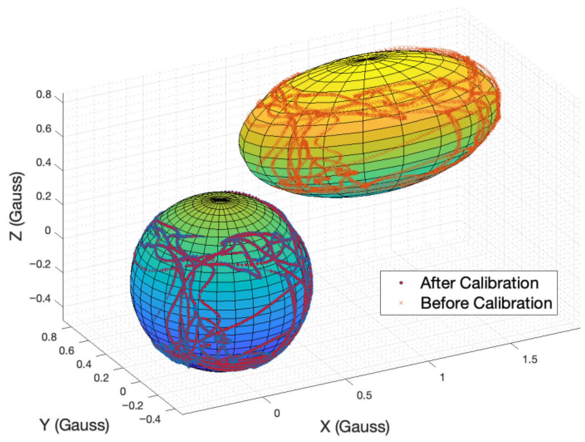
Considering hardware, the magnetometer is the greatest source of error, as the Earth’s magnetic field experiences various interference effects from common devices and objects. Hard iron effects arise from fixed, magnetized components within the device, resulting in a constant three-dimensional magnetic bias. Soft iron effects stem from ferromagnetic objects that distort the Earth’s magnetic field [29,30]. In most sensing applications, including this one, calibration of the magnetometer is necessary to achieve a desirable accuracy [31]. The data collected from calibration forms an ellipsoid cloud of measurements, offset from the origin. Since hard iron effects are constant in the phone’s frame, they shift the ellipsoid from the origin, while variable soft iron effects distort axes unevenly, skewing what would be a sphere into an ellipsoid. Calibration then involves sphere-fitting the cloud of data and shifting back to the origin, as seen in Figure 1 [29].
Google recommends that, to best calibrate a magnetometer, the user performs figure-8s with the device, allowing each of the 3 axes to rotate through the ambient magnetic field [32]. Experimental testing found that after 2–4 figure-8s, Android’s SensorManager (discussed later) consistently reports a high-calibration state for the magnetometer. As this metric does not correspond to the FOP, it was found empirically that the FOP output settles after 2–5 extra figure-8s. To ensure that the FOP was operating as intended, a minimum of 10 figure-8s were performed before data acquisition. This is what we will refer to as the calibrated state.
Figure 1.
Ellipsoid fitting for magnetometer calibration [33].
2.4. Custom Android App for Data Collection
To achieve a solution using orientation-based triangulation, data collection must involve recording the position, orientation, and timestamp. A specialized Android app was developed for this purpose. The app is primarily a camera view with a crosshair for the user to aim at targets. As this app is specialized for testing, it includes functionality to record data over time and to take individual “snapshots” of data. Data recording over time was used to track dynamic objects, while snapshot recording was used to simulate crowd sourcing for the static target. The prototype app is designed to record measurements at a sampling frequency of 1 Hz. A callback function is used to populate data whenever the FOP, which continuously runs in the background, detects a change in orientation. The FOP is capable of updating the orientation at a maximum rate of 200 Hz [28]. The callback ensures that our data-recording thread captures the most recent orientation estimate, and timing misalignment will be at the order of 5 to 10 ms. Time was synchronized across devices using the Network Time Protocol (NTP). In a conference paper from the University of Illinois at Urbana-Champaign, Hong et al. reported that standard NTP clients typically achieve a median synchronization error of 2 to 5 ms, though with a long-tail distribution under undesirable network conditions [34]. Relative to the 1 Hz app sampling rate used in this work, this timing uncertainty is small and was therefore not expected to be a dominant source of localization error. Time synchronization could remain a limitation for higher-rate or more time-sensitive applications.
The app also includes magnetic field and magnetometer calibration metrics to assist a user in achieving the best possible azimuth solution. The magnetic field metric displays the electromagnetic field magnitude in microtesla and tracks a window of recent consecutive measurements. It discourages the user from calibrating when the field strength is out of the Earth’s standard range, as well as if the field is excessively fluctuating within the window. The calibration metric is pulled from Android’s SensorManager API and provides an unreliable-, low-, medium-, and high-accuracy metric related to the magnetometer’s state. While this is insightful, it does not come from Android’s FOP, so while the magnetometer may be calibrated, the FOP may not be displaying the most accurate heading. An image of the resulting app is included in Figure 2.
Figure 2.
Specialized Android app.
2.5. Experimental Setup
The primary smartphone used for data collection in this research is the Google Pixel 6. The Pixel 6 was chosen because we had many at our disposal, which was necessary for large data collection. Additionally, this device is readily available to the public and is affordable, at less than $300 [35].
The first steps to understanding whether smartphones are feasible as a measurement platform involved analyzing their orientation accuracy. The initial device accuracy analysis was performed using landmarks with known locations. Knowing the location of the device and target allows for the calculation of accurate truth values for azimuth and elevation angles. Singular sets of data were taken in the calibrated state, primarily using the sun and moon as near-static targets. To further test the feasibility of locating a dynamic object, data was recorded at 1 Hz, tracking primarily commercial flights. Automatic Dependent Surveillance–Broadcast location data was pulled from online resources and linearly interpolated, allowing for the calculation of the true angle values.
To assess the feasibility of localizing a target, a static landmark visible from a large surrounding area was selected, as triangulation benefits from diverse planar and vertical geometry. The use of a static target also provided the capability to aggregate over 100 data points collected across several days, effectively simulating a singular event observed by many devices. This experimental setup additionally enables the solution to be evaluated as a function of the number of observers. Given that there are more than 5 billion Android smartphones worldwide, crowdsourcing a small fraction of nearby devices could plausibly provide an ample number of measurements. Accordingly, this experiment is structured to explore how solution quality scales with the number of available observations.
Following the localization of a static target, a dynamic localization test was performed to validate the intended use case of this research, localizing UASs. This test involved a more complex setup to aggregate measurements compared to the static localization experiment. With the goal to simulate collecting around 100 observations at each time epoch, it was essential to ensure repeatability in a drone’s flight path to allow measurements to be grouped. To accomplish this, a custom-built Tarot X6 hex rotor drone flew a repeated flight path following GPS waypoints with real-time kinematic positioning (RTK) corrections between two points. Using RTK, which provides 1 to 3 cm-level accuracy, effectively removed variability in the drone path, ensuring repeatability. Following this repeated flight plan, about 100 observers were simulated for both a forward and reverse flight track with eight phones. To aggregate measurements, individual phone data could be aligned with the start command in GPS time pulled from the drone’s logs. This allowed for an experiment comparable to the static localization test to be performed without the logistical complexity of coordinating 100 simultaneous observers.
During the test, the observers were dispersed in a straight line at approximately 30 m intervals under the drone’s flight path. The line of observers traveled together, roughly 40 m, between flights to develop a grid pattern. Note that this specific geometry was a result of usable space constraints and the observed maximum line of sight range being about 400 m. The drone began and finished its flight outside the observation grid, providing a more realistic representation of the use case as a drone approaches, passes over, and proceeds away from the observers. The results of these experiments will be discussed after the developed mathematical model for target localization is presented.
2.6. Localization Model
The fundamental basis for the localization algorithm is the use of line-of-site vectors from the phones to the target. These line-of-sight vectors are derived from the angular measurements collected from smartphones and related back to physical distances using a nonlinear least squares estimator. Although these measurements do not give distance explicitly, by looking for intersection points between multiple line-of-sight vectors with known origin points, a target can be localized.
The Earth-centered Earth-fixed (ECEF) vectors that define the position of the phone are denoted, as shown in Equation (1), as . This vector is simply collected from the smartphone global navigation satellite system solution. The position of the target and the relative vector between the target and phone are denoted as and , respectively, in Equations (2) and (3). The line of sight vector is defined in Equation (4) as the normalized relative vector between the target position and the phone position. This establishes the relationship between the line-of-sight vector and the distance between the phones and the target.
To take advantage of this model within a nonlinear least squares estimator, we can derive a Jacobian matrix, J, from with respect to the states, x, y, and z. This matrix, shown in Equation (5), expresses how the line-of-sight vector components respond to changes in the state, so changes in the relative vector between an observed and computed unit vector can be mapped to ECEF changes in the state.
Using a general formulation, the diagonal terms can be represented with Equation (6) as the partial derivative of component of vector with respect to a. The variable a is simply used to represent one variable, x, y, or z, of the state vector.
The off-diagonal terms can also be represented using the generic form in Equation (7). For the off-diagonal terms, they are the partial derivative of the component with respect to state b. In this case, a and b represent different state variables.
The final component that needs to be defined for the use of a nonlinear least squares estimator is the measurement model. Using the azimuth and elevation angles collected from the phones as yaw, , and pitch, , respectively, an alternate form of the line-of-sight matrix shown in Equation (8) can be defined which is a function of these angles. These angles are collected in the local east, north, up (ENU) frame, so they must be transformed to the ECEF frame using the standard ENU to ECEF rotation matrix, , as shown in Equation (9). This matrix is dependent on the latitude, , and longitude, , of the observer position [36].
By converting the measurements into a standard global frame like ECEF, the state update can be performed in said standard global frame and it is not necessary to deal with converting between ECEF and local ENU frames associated with each observer during the estimation process itself. If the computed vectors instead had to be converted into ENU or angular azimuth and elevation, vector rotations and potentially vector-to-angle conversions would have to be performed each iteration step per observer.
Pulling these pieces together, state updates, , in meters, can be computed using an iterative Newton–Raphson algorithm for nonlinear least squares by solving Equation (10).
Using the relative vector between the computed and measured unit vectors provides insight into the difference between the two, with the minimization of the relative vector corresponding to agreement between the measurements and the current state estimate. A smaller relative vector, with both its components and magnitude approaching 0, represents better agreement, while larger relative vectors will result in larger state updates. The relative vector magnitude is bounded between 0 and 2 as it is the difference between two unit vectors, but through the relation back to the ECEF state through the Jacobian matrix, a solution in a common global frame is capable of being acquired. To show how the use of the relative vector is minimized using the presented formulation, a simple simulation can be presented, which allows the state update to be seen. In this simulation, five perfect observers are set up around a target. These observers are between 100 and 200 m below the target, and spread out at distances from the target, ranging between 3 and 7 km. The resulting relative vector progressions for all five observers are shown in Figure 3a, with a diagram showing how a single observer-relative vector—observer three, which is represented in yellow in Figure 3a—changes during iterations 1 through 4 in Figure 3b. This figure shows how the components of the relative vector are minimized as the solution iterates and updates.
Figure 3.
(a) Simulated relative vector progression using the aforementioned state update technique. (b) Relative and computed vector progression for a single observer for iterations 1 through 4.
When concerned with potential error within the measurements, it is important to understand how the error propagates through the angle to the line-of-sight vector transformation. Analytically, this can be performed by starting with some observed or expected angular measurement errors, and for yaw and pitch, respectively. These values, in practice, would have to be found by surveying a smartphone model’s performance, as is done in Section 3.1 for the Google Pixel 6. Assuming that these two measurements are uncorrelated, a measurement covariances matrix can be set up, as seen in Equation (11).
Using the measurement model shown in Equation (8) before rotation into the ECEF frame, it is possible to convert this matrix into the unit vector space by leveraging the assumption that the azimuth and elevation measurements are uncorrelated. This means that errors in the line-of-sight vector for either the east, north, or up direction, represented generally as c, can be computed using Equation (12).
For the partial derivatives, these are computed using the conversion from angular to ENU line-of-sight vectors in Equation (8). To perform the conversion for all of the states, these derivatives can be grouped into a matrix, , as in Equation (13), which is then multiplied by the measurement covariance to get the resulting covariance matrix of the ENU unit vector. The rotation from the ENU frame to the ECEF frame using can also be included in the formulation in Equation (14) to get the unit vector errors in the ECEF frame, . It is important to note that the results for this are dependent on the azimuth and elevation uncertainties in the measurements, the measured azimuth and elevation value, and the position of the observer due to the frame rotation.
This formulation can be validated by performing a Monte Carlo analysis which visualizes how this linearized approach models the error propagation of random error in the angular measurements. An example of this Monte Carlo analysis is provided in Figure 4. In this analysis, a simulated observer is placed outside the University of Colorado Boulder Aerospace Engineering Sciences building. Three different standard deviations, 5, 10 and 15 degrees, were tested for the angular distributions, and the results for the all azimuth and select elevation values are included. In this analysis, equal azimuth and elevation random errors are used, and the Monte Carlo analysis contains 10,000 points. These plots in Figure 4 show that for random errors with a standard deviation at or under 10 degrees, as shown in Figure 4a,b, the linearized model does well to approximate the expected ECEF unit vector error. Above this value, the linearized model begins to degrade relatively quickly at 15 degrees, as shown in Figure 4c; significant differences in the linearized and Monte Carlo approximations are observed. This is noteworthy as a linearized error propagation model can be used, but it is important to recognize that a Monte Carlo approach may be necessary if the measurements have high uncertainties.
Figure 4.
(a) Monte Carlo and linearized measurement error propagation for azimuth and elevation error standard deviations of 5 degrees. (b) Monte Carlo and linearized measurement error propagation for azimuth and elevation error standard deviations of 10 degrees. (c) Monte Carlo and linearized measurement error propagation for azimuth and elevation error standard deviations of 15 degrees.
Using the measurement covariance matrix from Equation (14) alongside the final estimate of J the uncertainty of the solution of the nonlinear least squares estimator can be computed as shown in Equation (15). This provides some insight into the performance and confidence of the estimation based on the expected angular errors and positions of the observers. It is worth noting that the pseudo-inverse of , , must be computed as the original matrix is not invertible due to it being rank 2 instead of 3 on account of it being derived from the 2 × 2 angular measurement covariance matrix.
As a final note for this technique, the initial condition can be set to the average position of all the observers, and a Newton–Raphson formulation for the nonlinear least squares estimator was leveraged. The initial condition being set to the average position of the observers provides a nearby point for the estimator to begin at, and it is reasonable, as in order to get a measurement, the observers will all have line-of-sight on the target. The use of the Newton–Raphson approach provides the ability to converge more efficiently. For this approach to the the nonlinear least squares estimator, the value of is applied to the current state estimate to get . Then, the mean square error cost function shown in Equation (16) for n observers, , is computed at the new state estimate.
This is then compared to the cost value of the previous state estimate, . If the value of is less than , the nonlinear least squares estimator moves on to the next iteration. If the value of is greater than , the update is reduced by a factor of two, and are recomputed, and the values of the cost function are once again compared. This process can then be repeated, while remains larger than by continuing to reduce by factors of two.
2.7. Correction Techniques
To assist in generating a more accurate estimate of a target’s location, two correction techniques are put forward. The first of these is a regression-based correction to the collected azimuth measurements based on an observed directional bias within a smartphone model’s collected data. The second is a measurement curation technique, which looks at how the post-fit residuals of the measurements compare to the expected measurement covariance matrix and removes the measurements outside of the two sigma bounds.
As will be discussed during the smartphone measurement capability assessment in Section 3.1, a directional based bias was observed within the smartphone data. This bias will be discussed at greater length within that section, but it was noteworthy that the bias seemed to follow a periodic trend. To model this trend, a periodic regression could be performed on the azimuth errors with respect to truth, . If the periodic trend is modeled as a combination of a sine and cosine term, the resulting model solves for the regression coefficients and , which could then be used alongside a given azimuth value to approximate the bias present.
Due to the potential error sources, which include humans, calibration, and general sensor quality, it was desirable to develop a method which could remove some of these poor measurements to improve solution accuracy. The challenge arises in that the observers are in theory at different points around the target, producing unique azimuth and elevation measurements, and it is assumed that there is no guarantee that the observers would each be collecting more than a single measurement. Thus, attempting to remove the measurements before computing the solution runs the risk of removing good measurements, as it is difficult to determine what is a poor measurement without knowledge of the target location. If it is assumed that the majority of measurements are “accurate,” then it is expected that the nonlinear least squares solution should converge near the true target location. Using the post-fit residuals of the nonlinear least squares solution we can then identify poor measurements which show errors deemed significant. These can then be removed and the estimator can be run again.
To identify poor measurements, the residuals of the nonlinear least squares estimator can be compared to the ECEF unit vector uncertainties computed in . This requires some a priori estimates of and . The matrix can be computed for each observer and the diagonal terms can be pulled to get the expected uncertainty. Poor measurements can then be identified as those which have one or more post-fit residual component outside of the predicted values. Due to the lower-quality sensors and the introduction of human error, a more aggressive removal bound of was leveraged as opposed to . By curating the data to remove measurements which have poor post-fit residuals based on expected measurement uncertainty, we can attempt to deal with measurements that have significant human, calibration, or sensor errors.
3. Results
To provide a comprehensive assessment of the feasibility of smartphone-based aerial target localization testing, the results are broken down into three sections. These are an assessment of the measurement capability of smartphones, focusing primarily on the Google Pixel 6, the position estimate of a static target test, and the position estimates of a dynamic UAS target. The first simply looks at the measurement output by the smartphones under both static and dynamic conditions. These measurements were collected by looking at various targets and over numerous days.
3.1. Smartphone Measurement Capability Assessment
Before using smartphone measurements in a localization framework, we must quantify their accuracy and limitations. This section evaluates both the static and dynamic pointing accuracy of the Google Pixel using the FusedOrientationProvider. These results establish performance baselines and guide corrections applied in later localization tasks.
Initial static tests were performed using the Google Pixel and calibrated with 10 or more figure-8s. Measured azimuth and elevation, and , respectively, are pulled from the custom app, while the truth data, and , is calculated using the MATLAB 2025a Navigation Toolbox. The difference between the phone’s coordinates and the target’s coordinates is converted to ENU and then to azimuth and elevation angles using Equation (17). Root mean square error (RMSE) is used to report angular errors, as defined in Equation (18), where the equation shown can be modified to solve for azimuth by interchanging the appropriate terms in the equation with their azimuth equivalents. Static testing, performed by pointing at the sun, moon, and a nearby mountain peak, yielded the results in Table 1.
Table 1.
Static pointing error.
Analyzing the static pointing capabilities of modern smartphones provides a comparison to the capabilities of older-generation devices. A 2020 study by Dresden University of Technology in Germany reported azimuth errors of and in static and dynamic modes, respectively, [30]. This study was performed on smartphone models produced from 2013 to 2019 and used a variety of fusion techniques. Compared to our reported azimuth error of , there has been a significant improvement in the few years since 2019, encouraging further investigation. This improvement is attributed to the FOP and to improved sensor quality. These results also confirm accurate elevation measurements, as expected from a stationary accelerometer. This data additionally provides a performance baseline for the FOP to compare dynamic state data with.
Dynamic target testing was also performed using a calibrated Google Pixel. The goal of dynamic target testing was to understand the workings of the FOP and how accuracy may change over time. Combining the 1100 data points taken at 1 Hz from 21 tracked flights produced the results shown in Table 2. It will be discussed how the inclusion of bias removed RMSE indicates the input of human error.
Table 2.
Dynamic pointing error.
These values align closely with the static results, implying that the FOP performs similarly under both static and dynamic conditions. Comparing these results to those of the Dresden University study, it is clear that the FOP has made great leaps in terms of reporting an accurate azimuth in the dynamic mode. While the Dresden University study showed an error increase of nearly when moving from static to dynamic pointing, the FOP results presented in Table 1 and Table 2 only showed an approximately degradation. In addition to this, the dynamic FOP error of was still much smaller than the static pointing error previously seen in Android devices.
The differences between static and dynamic results were influenced by the fact that static testing allowed time to carefully align the crosshair with a target, reducing human input error. Dynamic testing, on the other hand, involved a significant amount of human inaccuracy, as holding the device steady while pointing at a far target proved difficult. Of the 21 dynamic data sets, 11 showed a constant azimuth bias, while the remainder had a constant drift. Because human pointing variability is not expected to appear as a nearly constant offset across an entire trial, the bias-removed azimuth RMSE is used here as an indicator of random user input error. Although this separation is approximate, it suggests that the underlying FOP performance in dynamic operation remains close to that observed in static testing. Examples of the constant-bias and drifting-error cases are shown in Figure 5a and Figure 5b, respectively.
Figure 5.
(a) Flight ASA414 signed angular error. (b) Flight UAL1470 signed angular error.
Figure 5a,b are representative examples of the constant azimuth bias and azimuth drift trends observed in the 21 dynamic sets. The figures show the signed error, defined as truth minus measurement, for both azimuth and elevation. In all sets, the difference in elevation angle is comparatively stable and falls within . In Figure 5a, aside from the spike attributed to human pointing error, the azimuth error remains near a constant bias of about throughout the 60 s recording. In Figure 5b, the azimuth error drifts from about , crosses zero, and approaches approximately . To further inspect this, data was recorded over time with a calibrated phone in a stationary position. These results are presented in Figure 6a,b, in which both constant azimuth bias and azimuth drift are observed. This suggests that the drifting behavior is unlikely to be caused primarily by changing device attitude or user operation during tracking. Rather, the behavior appears to be associated with the heading-estimation process itself. Because residual soft-iron effects after calibration would be expected to produce a fixed directional bias rather than time-varying drift in a stationary configuration, the observed behavior is more consistent with internal FOP fusion behavior and/or magnetometer weighting that is not exposed to the user. The nearly constant azimuth offsets are most consistent with a systematic heading bias, likely arising from residual magnetometer error within the fused orientation estimate. The exact mechanism remains an open point and is left for future work, but these results show that the FOP can still exhibit azimuth limitations in precision applications.
Figure 6.
(a) Constant bias case, stationary azimuth test. (b) Drifting case, stationary azimuth test.
The aggregated measurement distribution and statistics from dynamic tracking and static localization are provided in Figure 7 and Table 3. Each data set has been analyzed separately up until now, where we look at the combined distribution. In Figure 7, the boxes outline the inner 50% of data points and contain a red median line. The whiskers extend to the high and low ends of the range, while the red + signs are outliers. Figure 7 shows signed error (truth-measured) while the RMSE statistics of these distributions are included in Table 3.
Figure 7.
Aggregated static and dynamic signed angular error box plot.
Table 3.
Angular RMSE of aggregated static and dynamic measurements.
Since we know the static and dynamic cases perform similarly, by combining the largest data sets, we can see the most comprehensive error distributions. The combined plots in Figure 7 exhibit slightly biased, unimodal distributions with large tails. The large tails and increased RMSE can be attributed in part to the addition of new testers and ambiguous targeting. One target was a mountain peak providing a large region to point at, specifically increasing the positive tail in the elevation distribution. Considering the azimuth distribution, the majority of the error falls within and is centered around . Since the bulk of the distribution is centered, localization may average out this error. It is also worth noting that nearly half of the data was taken facing west, which could attribute the centering to a directional azimuth error trend mentioned below.
The final point of interest is the assessment of a measurement trend noticed in the dynamic pointing test. The observation was that in sets looking primarily south, azimuth is generally underestimated, while in sets looking primarily north, azimuth is generally overestimated. Recall that azimuth is measured clockwise with being true north, being east, and so on. Hence, azimuth measurements tend to drift east. To analyze this trend in depth, the bias-removed azimuth error of the static localization data was plotted against the azimuth truth. The resulting plot presented below, Figure 8a, was smoothed into bins, and a periodic regression was fit.
Figure 8.
(a) Google Pixel directional azimuth error. (b) Device-specific directional azimuth error.
The smoothed data indicates a strong correlation between the pointing direction and azimuth measurement error. A working hypothesis for this behavior is residual soft iron interference after calibration. In this interpretation, the calibration process does not fully capture the soft iron distortions introduced by smartphone internal components in every direction, and the Earth’s magnetic field is skewed differently depending on the angle it passes through phone components. This produces a directional error pattern that is well approximated by a sinusoidal trend.
This hypothesis further suggests that the error trend is device-specific, since different models will have different internal component layouts and magnetic environments. To examine this point qualitatively, limited testing of the Samsung Galaxy S24 and Xiaomi X14T devices was performed alongside the Google Pixel 6. Figure 8b shows sinusoidal regressions fit to the bias-removed azimuth error for each device. The clear phase differences between these regressions support the interpretation that the directional azimuth error trend is not universal across phones, but instead depends on device-specific hardware characteristics. However, the localization experiments in this study were conducted with the Google Pixel 6 device, so the reported positioning results should be interpreted in that context rather than as a cross-device generalization.
An additional limitation is that this behavior will not only depend on the phone model, but also any additional accessories, as these may alter the effective magnetic environment and therefore change the azimuth bias pattern for a given phone. Although magnetometer calibration is expected to be capable of handling some of these effects, this is left for future work. As a result, the directional correction described here should be viewed as device- and configuration-specific. In the context of a crowdsourced solution, the ability to aggregate large numbers of observers should help to minimize the impact of these special cases.
3.2. Static Target Localization
As previously mentioned, a static landmark was chosen which was easy to identify from around Boulder, Colorado. The chosen target was the top of Darley North, highlighted in Figure 9, a tower in the south of Boulder which rises above the majority of the Boulder skyline. The true position of this target was obtained by collecting GPS data from the point of interest shown below. Beginning with a static target provided a known, easy-to-identify object which served as the first level of verification for the localization algorithm.
Figure 9.
Target for static localization, Darley North dorms [37].
To collect data to localize this target, members of the Radio Frequency and Satellite Navigation Laboratory at the University of Colorado Boulder were asked to travel around Boulder, Colorado. Each member was given a smartphone and was tasked with finding spots around Boulder where the static target was visible. Once a location was found, the user would open the custom app, calibrate, and then record a snapshot while looking at Darley North. As the target was stationary, data points could be treated as if they were taken at the same time. The resulting spread of data points is shown in Figure 10.
Figure 10.
Spread of measurements observing Darley North.
Estimating the position of Darley North from these data points results in the following solution in Figure 11 with the error in Table 4. Furthermore, included in this table is the 3D uncertainty derived from the covariance matrix and the ENU uncertainties derived from the diagonal of the ECEF-to-ENU-rotated covariance matrix. The resulting solution using all of the collected measurements was relatively inaccurate at nearly 30 m of error, but the use of correction techniques showed promise in producing better results.
Figure 11.
Darley North localized solution.
Table 4.
Error and uncertainty of Darley North solution.
The two correction techniques outlined in Section 2.7 were used to improve the solution. For the results presented in this paper, regression coefficients of equal to 3.45, and equal to −2.73 based on the results in Figure 8a, were used. When using the measurement curation, and of 9.28 and 3.60 degrees, respectively, were used to compute the observer matrices. These values were obtained by using the aggregate static and dynamic data discussed in Section 3.1 after accounting for the directional bias. Table 5 gives the static target position estimate error and estimator uncertainty when these two methods are applied both independently and together. For both the independent and combined cases, the measurement curation technique flagged and removed about 23.33% or 28 of the 120 measurements.
Table 5.
Error and uncertainty of Darley North solution when using correction techniques.
The results in the table show that the correction techniques can produce a better solution, albeit with slightly larger uncertainty due to the reduced measurement count. An improvement is seen when using each of the correction methods on their own, and an even more significant improvement is observed when they are used together. The combined improvement is just under 20 m when compared to the baseline solution, and would indicate that in this case not only is the directional bias impacting the results, but that there are a number of very poor measurements that also have a large influence on the solution. This can be verified by looking at the difference between the measurements and the true angles, as shown in Figure 12a,b, as well as the residuals before and after using the curation, as shown in Figure 13a,b.
Figure 12.
(a) Difference between measurements and truth before data curation. (b) Difference between measurements and truth after data curation.
Figure 13.
(a) Residuals of target localization before data curation. Each line represents the residual progression of an individual observer. (b) Residuals of target localization after data curation. Each line represents the residual progression of an individual observer.
In Figure 12a, several poor elevation measurements are readily identifiable by the elevation differences being in excess of 10 degrees, and for azimuth, several poor measurements sit in excess of 20 degrees. The impact of these measurements is seen in the residual plot of Figure 13a, where several norms of the residual line-of-sight vectors are large, indicating poor agreement between the observed and computed measurements. By applying the measurement curation and regression, the results in Figure 12a,b are produced, which show the elimination of some of the outlier measurements and much better residuals. Specifically, in the elevation plots, the large positive errors in excess of about 10 degrees are eliminated, while the azimuth error is now constrained to between −15 and 15 degrees.
The two corrective methods outlined in this section, and their resulting impact on the static target solution, show great promise for crowdsourced smartphone target localization. They can effectively remove measurements that show poor alignment with true pointing values, as shown in Figure 12, and assist in correcting previously observed directional biases. Their final impact on the static target highlights this as the solution error saw a significant reduction from 31.38 m to 11.60 m using human recorded measurements with sensor platforms not designed for this purpose.
3.3. Dynamic Target Localization
With confidence that a static target can be localized down to below 12 m of accuracy, a test looking at the application of the discussed model to the target use case of a dynamic drone was performed. This test, as described in Section 3, involved tracking a drone following a repeated autonomous flight path. The forward and reverse tracks alongside the smartphone observer locations are shown in Figure 14a,b. In these plots, the drone travels from dark blue to yellow.
Figure 14.
(a) Forward drone track and smartphone observer locations. (b) Reverse drone track and smartphone observer locations.
Of note in these tracks is that the drone always begins and ends outside of the region containing the smartphones. As the geometry of the observers with respect to the target will be poor in these areas, it is expected that the accuracy in those locations will degrade and that uncertainty in the estimate will increase.
After running the collected phone data through the localization algorithm, the resulting solution estimates can be overlaid on the previous truth and observer plots. These results are shown in Figure 15a,b. The overlaid estimates show good qualitative agreement with the truth tracks, especially when the drone is within the region bounded by the smartphone observers.
Figure 15.
(a) Forward track localization estimates. (b) Reverse track localization estimates.
To gain a better understanding of the quantitative accuracy of the resulting location estimates, the east, north, up, and 3D error, as well as estimator uncertainty, can be plotted as a function of time.
Looking at the 3D error in Figure 16a,b, it can be seen that the bounded 3D accuracy of the solution for the forward track is between 5 and 10 m, while the reverse track is slightly worse, with bounded error between 10 and 20 m. Including the unbounded points increases the average error over the tracks to about 15 m for the forward test and approximately 21 m for the reverse track. Using Figure 17a,b, the average bounded east, north, and up error over the course of both the forward and reverse tracks can be assessed. It can be seen that, aside from the east error for both the reverse and forward direction at over 20 and 10 m, respectively, all of the average errors fall under 5 m. Once again, the points within the bounded region show better accuracy, especially for the east error.
Figure 16.
(a) Forward track 3D error. (b) Reverse track 3D error.
Figure 17.
(a) Forward track east, north, and up error. (b) Reverse track east, north, and up error.
Looking qualitatively at all four plots, it becomes evident that geometry plays a role in the solution accuracy. The largest errors generally occur before the drone enters or after leaving the area bounded by the observing smartphones. Additionally, when looking at the one sigma bounds, it can be observed that poor geometry can have a significant impact on our confidence in the state estimate. At the farthest points outside of the bounded region, the uncertainty is above 10 m both for the 3D and east component as a result of the poor east–west geometry in these regions. As the drone approaches the bounded region, the uncertainty improves, dropping below 5 m once within the bounded region, before once again beginning to increase as the drone flies away from all of the observers. Referring back to Figure 14, the flight path extends further outside the observation grid to the east, which is reflected in the increased error on one side of each of the four plots. Instances of entering and exiting the boundaries are marked on the plots by the red dashed line and green dashed line, respectively. The impact of these regions on the resulting error estimates and uncertainty can be seen in Table 6.
Table 6.
Average error and average uncertainty of dynamic tests with and without target outside observer bounded region.
As noted when looking at the static target, there are techniques that can be leveraged to improve the solution without requiring a priori knowledge of the true target location. For these techniques, the same parameters leveraged in Section 3.2 for the static target are used for the dynamic drone. For the measurement curation, it is worth noting that this was performed per epoch and generally resulted in only 2 to 5% of measurements being removed on average, indicating generally better measurement quality in this test compared to the static test.
The results of applying the regression, measurement curation and both techniques together on both the forward and reverse tracks are shown in Table 7 and Table 8. Additionally, as in Table 6, the average errors and uncertainties have also been estimated for the case where the drone is only within the observer bounded region.
Table 7.
Forward average error and average uncertainty of dynamic test when applying correction techniques.
Table 8.
Reverse average error and average uncertainty of dynamic test when applying correction techniques.
As with the static test, we can see that the inclusion of the correction techniques provides benefits to the resulting accuracy of the solution, and in this case, also to confidence in our state estimate, as seen in the uncertainties. In the case of the forward track, the inclusion of both regression and measurement curation improves the average 3D accuracy from about 15 m to just under 10 m. However, it is worth noting for the forward track that when only considering the target track bounded by the observers, the solution accuracy does not show much improvement. All of the solutions are within a meter of each other, which may indicate that at this point, small human error or sensor quality becomes the limiting factor to solution accuracy. The reverse track also shows less, but still notable, improvement when comparing the solution without correction techniques to the solutions with correction techniques. Unlike the forward track, an improvement is seen when looking at the bounded and unbounded solution, as the combined correction technique reduces both the unbounded results by about 9 m, while the bounded region results improve by approximately 4 m.
4. Discussion
Comparison to Simulation
To provide further confidence in the experimental results, a comparison can be made to a simulated output. For the simulation, the measurements were generated from the known truth position of the target and the positions of the phones. The measurement distributions were assumed to have mean values equal to the “truth” bearings, while the standard deviation for angular measurements was chosen as 9.28° for azimuth and 3.6° for elevation. These are the same values used for the measurement curation that were derived from the directional bias-removed aggregate static and dynamic smartphone assessment data. The directional bias observed in Figure 8 was also incorporated into the simulation measurements to best match the experimental setup. Each simulation was run several times, with each run having a new set of measurements drawn from the predefined distributions.
The resulting average error of 100 simulations of the static target localization was approximately 21.71 m, with a standard deviation of approximately 8.08 m. This value was in the same order of magnitude as the solutions seen in the previous sections, and the uncertainty was also nearly equivalent to the observed uncertainty in the nonlinear least squares solution. Although the experimental solution performs worse than the simulation without correction techniques, when they are included, the resulting experimental solution performs better than the simulation. This result is due to human error that can introduce large erroneous measurements, albeit not with a high frequency. The two correction techniques alleviate the impact of not only these large human biases through measurement curation, but also smaller directional biases introduced into the measurements. In particular, the measurement-curation-only solution is worth comparing against. In this case, the directional bias is still included, while poor measurements that would not be captured by the simulated measurements have been removed. The experimental uncertainty has increased due to the lower number of observations, but the solution error itself is under five meters in difference from the simulation.
Another benefit provided by the simulation was the ability to easily assess how the number of phones influences the resulting solution. For the static target, the number of available observers was varied between three and one hundred and nineteen. The upper threshold of one hundred and nineteen corresponded to the total number of experimental static target measurements taken, with the associated positions of the observers from the experimental test provided to the simulation. For each selected number of available observers, 100 simulations were run, which randomly drew the selected number of observers from the pool of available observers. This meant that 100 geometries were tested for each number of available observers. Duplicate locations were not chosen within a simulation. The solution with varying numbers of monitoring stations or observers for the simulations is shown in Figure 18a,b for the static target. The key difference between these plots is that for Figure 18a, the simulation uses the simulated zero mean, azimuth and elevation standard deviation measurements, while for Figure 18b, the simulation draws from the experimentally collected measurements.
Figure 18.
(a) Simulated expected accuracy as a function of measurement number for the static target. (b) Experimental expected accuracy as a function of measurement number for the static target.
From these static plots, it immediately becomes evident that there is a decreasing return on accuracy as you increase the number of observers for the orientation estimation performance currently observed. For both the experimental and simulation results, an exponential decay in 3D error can be seen. Although the resulting accuracy becomes more stable as the number of observers increases, which is seen in the continued decrease in the standard deviations, the average error levels off after about 30 observers. The average error limit of the plot is a function of the phone position and angular measurement error introduced. The uncertainties follow a similar trend as well, with the values beginning to asymptote around the same point as the errors. Finally, it is worth noting that the experimental results do not asymptote to the same points as the simulation results. This is primarily due to the human bias caused by an observers attempts to aim at the static target and sensor biases present in the collected measurement distributions, as well as a lack of correction techniques, resulting in Figure 18b. Despite this, the experimental results follow similar trends to the simulation results, providing a strong correlation between simulation and application as the errors and uncertainties often fall within a several meters of each other.
Further exploring how the geometry impacts the resulting solution, the simulation could be adjusted to look at how the position dilution of precision (PDOP) and number of observers affects the resulting solution accuracy. The PDOP is computed from the dilution of the precision matrix, , which is estimated from the true line-of-sight vectors between the known observer positions and the true target location, with lower PDOP representing better geometry. This metric has been used extensively for position, navigation, and timing applications, such as GPSs, to gain an understanding of how geometry may impact positioning accuracy. The method to compute this metric is shown in Equations (19) through (21) where the line-of-sight matrix for n observers, , comprising line-of-sight vectors computed using Equation (4), transposed, and stacked on top of each other.
For this simulation case, random positions were drawn uniformly from a 2 km by 2 km north-east region centered around a target. This was similar to where the majority of experimental observations were collected for the static experiment. The up component of the observer position was drawn from a uniform distribution centered 60 m below the target with a range of 170 m around that center. This meant that most observers were looking up at the target while a handful could be generated to be at the same level or above the target as was the case in the static test. The same noise characteristics for the measurements, as in the simulation for Figure 18a, were leveraged, and the directional bias was included. Finally, the simulation was run 100 times for each observer count in the range of 3 to 110.
The resulting simulation results as well as a similar plot generated using the experimental observers and measurements is included in Figure 19a,b. The difference in the appearance of these plots is due to the limited observer set that the experimental results can pull from in comparison to random simulated observer sets, which change each run. In both of these plots, the red line is a moving average taken over the data points to help show how geometry can influence the solution, as better geometries generally correspond to better solutions. The most interesting point that both of these plots display that although there can still be variation in the resulting solution accuracy with good geometries, the accuracy generally improves, as shown by the red average lines. Additionally, the number of observers is seen to increase the quality of the geometry, as shown by green and yellow points, representing a higher numbers of observers, corresponding to lower PDOP values, and thus lower average error.
Figure 19.
(a) Simulated expected accuracy vs. position dilution of precision and observer count. A moving average, the red line, has been included in the plot to show the trend in how accuracy changes with geometry. (b) Experimental expected accuracy vs. position dilution of precision and observer count. A moving average, the red line, has been included in the plot to show the trend in how accuracy changes with geometry.
For the dynamic target, a similar assessment can be performed using the simulation. As the dynamic target was solved point-wise, the expectation was that results should be similar to the static localization simulation results. What the dynamic target does allow for is an exploration of how a target outside the region bounded by observers can be compared to a target within the region bounded by observers. To simplify this simulated analysis, two points were chosen to be assessed, only the forward track was considered, and the number of potential observers varied from three to one hundred. For the chosen points, one was selected that was within the region bounded by the observers seen in Figure 14a, while the other was selected outside the bounded region. The chosen points were at 00:01:04 s into the forward track for the bounded point and 00:01:34 s for the unbounded point. Furthermore, since the forward and reverse tracks should perform similarly, including results from the reverse track was considered unnecessary.
Looking at the resulting dynamic target simulation accuracy, we can see that for ninety-three devices observing the bounded point, the average accuracy is 5.04 m with a standard deviation of 1.43 m. Compared to the results of the bounded region in Table 6 and Table 7, the simulated solution is slightly worse than the average errors seen for a bounded point. Compared specifically to the solution at the time of interest, without any correction techniques, the solution was 5.49 m, which is larger than the simulated result. In both of these cases, the uncertainties of the experimental solution are slightly larger at 2.04 m from Table 6 and 1.89 m for the exact point. If correction techniques are applied, the experimental result can improve to 2.98 m with an uncertainty of 1.41 m. These average error values do both fall within two standard deviations of the simulated results, and the uncertainties are similar, but the discrepancy in the results highlights the variability that measurements can introduce to the solution. For the point that was not bounded by the observers, ninety-three measurements were also used in the experimental solution. The average and standard deviation of the errors were 17.75 m and 5.87 m, respectively. This is in comparison to the experimental result for this time, which had an error of 40.17 m and uncertainty of 10.19 m. Even when including the correction techniques, this solution only improves to about 20.97 m with an uncertainty of 3.49 m. The poor measurements and geometry of the experiment for the unbounded point in this case cause the large, nearly two times, discrepancy between the experimental and the simulated error results. Even when the estimator has a lower uncertainty in this case the actual observed error is larger. Looking at the averages from the tables, when including points outside the bounded region, these are more in-line with the unbounded point solution ranging from 9 to 15 m based on the inclusion or exclusion of the correction techniques. Figure 20a,b show the simulation results for the accuracy as a function of observers for the chosen points. These show a very similar behavior to the static point test, with the exponentially decaying relationship between accuracy and observer count evidently displayed.
Figure 20.
(a) Simulated expected accuracy as a function of measurement number for the dynamic target at time 00:01:02. (b) Simulated expected accuracy as a function of measurement number for the dynamic target at time 00:01:34.
5. Conclusions
This paper aims to evaluate the capability and feasibility of using smartphones as dispersed optical measurement platforms for small aerial drone localization. A custom Android app was built to collect measurements, and the use of a nonlinear least squares estimator based on line-of-sight vectors provided the means to convert angular measurements to ECEF target position coordinates. The results within this work show the promise of using the low-cost, widely available sensors available in smartphones to localize a single static and dynamic target to within 12 m. The lower quality of the sensors make the use of solution correction techniques necessary to achieve these accuracy levels. In this paper, two correction techniques were presented: a regression based on measurement trends observed during the smartphone measurement exploration and a measurement curation based on looking at post-fit residuals and expected measurement uncertainty. To apply the regression, the smartphone model must be known, and for measurement curation, prior testing with the phones is necessary to establish expected angular errors.
The single drone localization work presented within this paper lays the foundation for future research surrounding the topic of crowdsourced drone localization. Notably, the extension or adaptation of the proposed crowdsourced technique to the case of multiple-drone localization, highly dynamic drones, or sparsely observed drones would be of particular interest. The research within this paper assumed only a single, predictable, dynamic drone, which may not always be the case in a real-world scenario. To extend this work to the multiple-drone scenario, what would be of utmost importance is either determining methods to appropriately group measurements before estimating each of the groups’ target position, or the development and application of an estimation algorithm, which can provide multiple unique drone state estimates. In the case of highly dynamic or sparsely observed drones, as could be possible in urban or obstructed scenarios, it is possible that there may be less available measurements for a given time or that those measurements are of lower quality. This may be due to human error as observers attempt to measure a highly dynamic or obscured target, or calibration errors as observers have to react to an agile drone. In this case, pairing the proposed crowdsourced method with an appropriate dynamic system model may be necessary to allow the technique to continue to track these more difficult drone targets.
With the growing potential for disruptions that small UASs can cause, the capability to localize them becomes increasingly important to enabling swift responses. The development of higher-grade observation tools could enable more accurate measurements and thus localization solutions but smartphones present an already widespread platform that if leveraged do not necessitate specialized hardware to perform localization.
Author Contributions
Conceptualization, D.A.; methodology, J.R. and F.T.III; software, J.R. and F.T.III; validation, J.R. and F.T.III; formal analysis, F.T.III; investigation, J.R. and F.T.III; resources, D.A.; data curation, J.R.; writing—original draft preparation, J.R. and F.T.III; writing—review and editing, D.A., J.R., and F.T.III; visualization, F.T.III; supervision, D.A. and F.T.III; project administration, D.A.; funding acquisition, D.A. All authors have read and agreed to the published version of the manuscript.
Funding
This research received no external funding.
Data Availability Statement
The raw data supporting the conclusions of this article will be made available by the authors on request.
Acknowledgments
The authors of this paper would like to thank Penina Axelrad from the University of Colorado Boulder for lending the Tarot X6 hex rotor drone to the members of the Radio Frequency and Satellite Navigation Laboratory for the experimental testing performed in this work. Additionally, the authors would like to thank Alexander Kenyon from the University of Colorado Boulder for providing technical support for setting up and flying the aforementioned drone.
Conflicts of Interest
The authors declare no conflicts of interest.
References
- Ariante, G.; Del Core, G. Unmanned Aircraft Systems (UASs): Current State, Emerging Technologies, and Future Trends. Drones 2025, 9, 59. [Google Scholar] [CrossRef] [Scilit]
- Colomina, I.; Molina, P. Unmanned aerial systems for photogrammetry and remote sensing: A review. ISPRS J. Photogramm. Remote Sens. 2014, 92, 79–97. [Google Scholar] [CrossRef] [Scilit]
- Quero, C.O.; Martínez-Carranza, J.; Saldaña, D.; Mondragón, I.F. Unmanned aerial systems in search and rescue: A global perspective on current challenges and future applications. Int. J. Disaster Risk Reduct. 2025, 118, 105199. [Google Scholar] [CrossRef] [Scilit]
- Basso, M.; Soares Guimaraes, C.S.; Martini Da Rosa, A.; Morgan Pereira, P.H.; Pignaton de Freitas, E. Current and Future Perspectives on Drone-Based Computer Vision for Precision Agriculture. In Proceedings of the 2025 IEEE Latin Conference on IoT (LCIoT); IEEE: Piscataway, NJ, USA, 2025; pp. 270–273. [Google Scholar] [CrossRef] [Scilit]
- Dhamankar, N.; Kulkarni, P.; Dixit, N. Estimating Potential Solar Energy on Rooftops using Unmanned Aerial Vehicle. In Proceedings of the 2019 International Conference on Computational Intelligence and Knowledge Economy (ICCIKE); IEEE: Piscataway, NJ, USA, 2019; pp. 275–278. [Google Scholar] [CrossRef] [Scilit]
- Hodgson, J.C.; Baylis, S.M.; Mott, R.; Herrod, A.; Clarke, R.H. Precision wildlife monitoring using unmanned aerial vehicles. Sci. Rep. 2016, 6, 22574. [Google Scholar] [CrossRef] [Scilit]
- Emerging Aviation Entrants: Unmanned Aircraft System and Advanced Air Mobility; FAA: Washington, DC, USA, 2024. Available online: https://www.faa.gov/dataresearch/aviation/aerospaceforecasts/uas-and-aam.pdf (accessed on 9 February 2026).
- BBC News. Gatwick Airport: Drones Ground Flights. BBC, 20 December 2018. Available online: https://www.bbc.com/news/uk-england-sussex-46623754 (accessed on 30 March 2026).
- Deliso, M. Drone Operator Charged for Hitting ‘Super Scooper’ Plane During Palisades Fire: DOJ. ABC News, 31 January 2025. Available online: https://abcnews.com/US/drone-operator-charged-hitting-super-scooper-plane-palisades/story?id=118313936 (accessed on 30 March 2026).
- Gozzi, L. How Ukraine Carried Out Daring ’Spider Web’ Attack on Russian Bombers. BBC, 2 June 2025. Available online: https://www.bbc.com/news/articles/cq69qnvj6nlo (accessed on 9 February 2026).
- Goncharova, O. Russia’s Short-Range Drone Strikes Cause Over 3000 Civilian Casualties in Ukraine, UN Reports. The Kyiv Independent, 27 June 2025. Available online: https://kyivindependent.com/relentless-drone-strikes-cause-over-3-000-civilian-casualties-in-ukraine-un-reports/ (accessed on 9 February 2026).
- McNabb, M. The Silent Invasion: How Israel’s Small Drones Infiltrated Iran. Dronelife, 23 June 2025. Available online: https://dronelife.com/2025/06/23/the-silent-invasion-how-israels-small-drones-infiltrated-iran/ (accessed on 9 February 2026).
- Stewart, D.; Lushenko, P. Countering Small Drones: Office Works Toward Joint Solutions to Growing Threat; Association of the United States Army: Arlington, VA, USA, 2025; Available online: https://www.ausa.org/articles/countering-small-drones-office-works-toward-joint-solutions-growing-threat (accessed on 9 February 2026).
- Gordon, C. Air Force Chief: Small Drones Are Both ‘Threat and Opportunity’. Air and Space Forces Magazine, 29 October 2024. Available online: https://www.airandspaceforces.com/air-force-chief-small-drones-threat-opportunity/ (accessed on 9 February 2026).
- Yousaf, J.; Zia1, H.; Alhalabi, M.; Yaghi, M.; Basmaji, T.; Al Shehhi, E.; Gad, A.; Alkhedher, M.; Ghazal, M. Drone and Controller Detection an Localization: Trends and Challenges. Appl. Sci. 2022, 12, 12612. [Google Scholar] [CrossRef] [Scilit]
- Castrillo, V.U.; Manco, A.; Pascarella, D.; Gigante, G. A Review of Counter-UAS Technologies for Cooperative Defensive Teams of Drones. Drones 2022, 6, 65. [Google Scholar] [CrossRef] [Scilit]
- İsmail, G.; Ozgur, O.; Yavuz, Y.; Hani, M.; David, M. Detection, localization, and tracking of unauthorized UAS and Jammers. In Proceedings of the 2017 IEEE/AIAA 36th Digital Avionics Systems Conference (DASC), St. Petersburg, FL, USA, 17–21 September 2017; pp. 1–10. [Google Scholar] [CrossRef] [Scilit]
- Güzey, N. RF Source Localization Using Multiple UAVs through a Novel Geometrical RSSI Approach. Drones 2022, 6, 417. [Google Scholar] [CrossRef] [Scilit]
- Rei, R.; Yiftach, R.; Yuval, S.; Nahum, N. Experimental Results of UAS Localization and Tracking by Passive TDoA. In Proceedings of the 2024 IEEE International Conference on Microwaves, Communications, Antennas, Biomedical Engineering and Electronic Systems (COMCAS), Tel Aviv, Israel, 9–11 July 2024; pp. 1–6. [Google Scholar] [CrossRef] [Scilit]
- Graff, D.; Anderson, B.; Buck, D.; Peterson, C.K.; McLain, T.W.; Warnick, K.F. Online Calibration for Networked Radar Tracking of UAS. J. Intell. Robot. Syst. 2024, 110, 163. [Google Scholar] [CrossRef] [Scilit]
- Morris, P.J.B.; Hari, K.V.S. Detection and Localization of Unmanned Aircraft Systems Using Millimeter-Wave Automotive Radar Sensors. IEEE Sens. Lett. 2021, 5, 6001304. [Google Scholar] [CrossRef] [Scilit]
- Rudys, S.; Laučys, A.; Ragulis, P.; Aleksiejūnas, R.; Stankevičius, K.; Kinka, M.; Razgūnas, M.; Bručas, D.; Udris, D.; Pomarnacki, R. Hostile UAV Detection and Neutralization Using a UAV System. Drones 2022, 6, 250. [Google Scholar] [CrossRef] [Scilit]
- Tang, Z.; Ma, H.; Qu, Y.; Mao, X. UAV Detection with Passive Radar: Algorithms, Applications, and Challenges. Drones 2025, 9, 76. [Google Scholar] [CrossRef] [Scilit]
- Boddhu, S.K.; McCartney, M.; Ceccopieri, O.; Williams, R.L. A collaborative smartphone sensing platform for detecting and tracking hostile drones. In Proceedings of the SPIE Defense, Security, and Sensing, Baltimore, MD, USA, 29 April–3 May 2013. [Google Scholar] [CrossRef] [Scilit]
- Ericsson. Key Figures—Ericsson Mobility Report; Ericsson: Stockholm, Sweden, 2025; Available online: https://www.ericsson.com/en/reports-and-papers/mobility-report/key-figures (accessed on 30 March 2026).
- Counterpoint Research. Global Smartphone OS Market Share: By Quarter; Counterpoint Research: Hong Kong, China, 2026; Available online: https://www.counterpointresearch.com/en/insights/global-smartphone-os-market-share (accessed on 30 March 2026).
- Android 16 Compatibility Definition. Android Open Source Project. Available online: https://source.android.com/docs/compatibility/16/android-16-cdd#22_handheld_requirements (accessed on 9 February 2026).
- Introducing the Fused Orientation Provider API: Consistent Device Orientation for All. Android Developers Blog. Available online: https://android-developers.googleblog.com/2024/03/introducing-fused-orientation-provider-api.html (accessed on 9 February 2026).
- Magnetometer Hard & Soft Iron Calibration; Vectornav: Dallas, TX, USA; Available online: https://www.vectornav.com/resources/inertial-navigation-primer/specifications--and--error-budgets/specs-hsicalibration (accessed on 10 February 2026).
- Melanie, E.; Hans-Gerd, M. Investigation of Multi-Sensor Fusion Strategies for Improved Orientation Determination in Mobile Phone Imaging Applications. ISPRS Ann. Photogramm. Remote Sens. Spat. Inf. Sci. 2020, V-1-2020, 181–187. [Google Scholar] [CrossRef] [Scilit]
- Papafotis, K.; Nikitas, D.; Sotiriadis, P.P. Magnetic Field Sensors’ Calibration: Algorithms’ Overview and Comparison. Sensors 2021, 21, 5288. [Google Scholar] [CrossRef] [Scilit] [PubMed]
- Find & Improve Your Location’s Accuracy in Google Maps; Google: Mountain View, CA, USA; Available online: https://support.google.com/maps/answer/2839911?co=GENIE.Platform%3DAndroid&oco=1&sjid=4299862202209836620-NC#calibrate_phone_android&zippy=%2Ccalibrate-your-phone-or-tablet (accessed on 10 February 2026).
- Hu, X.; Wu, J.; Xue, B.; Zhu, Y.; Jia, M.; Qi, Y.; Jiang, Y.; Tan, P.; Zhang, W. AM-Align: Globally Optimal Estimation of Accelerometer-Magnetometer Misalignment. IEEE Trans. Instrum. Meas. 2024, 74, 1010710. [Google Scholar] [CrossRef] [Scilit]
- Hong, C.-Y.; Lin, C.-C.; Caesar, M. Understanding Root Causes of Internet Clock Synchronization Noise. In Proceedings of the Passive and Active Measurement, Atlanta, GA, USA, 20–22 March 2011; pp. 204–213. Available online: https://caesar.cs.illinois.edu/papers/csync.pdf (accessed on 10 April 2026).
- Google Pixel 6 5G, US Version, 128GB, Stormy Black—Unlocked (Renewed). Amazon.com. Available online: https://www.amazon.com/Google-Pixel-Unlocked-Smartphone-Ultrawide/dp/B09NP6697R/ref=pd_lpo_d_sccl_1/140-3318707-6134615?pd_rd_w=Zajmw&content-id=amzn1.sym.4c8c52db-06f8-4e42-8e56-912796f2ea6c&pf_rd_p=4c8c52db-06f8-4e42-8e56-912796f2ea6c&pf_rd_r=5EW8E4JHDW70S9V7GRNG&pd_rd_wg=BiDFD&pd_rd_r=9239d5f8-cdcf-40d8-b0fc-c098faf680c7&pd_rd_i=B09NP6697R&th=1 (accessed on 17 February 2026).
- Transformations Between ECEF and ENU Coordinates; ESA Navipedia: Madrid, Spain, 2022; Available online: https://gssc.esa.int/navipedia/index.php/Transformations_between_ECEF_and_ENU_coordinates (accessed on 11 February 2026).
- Darley North Hall. University of Colorado Boulder: University Housing and Residential Life. Available online: https://www.colorado.edu/living/housing/undergraduate-housing/explore-housing/darley-north-hall (accessed on 10 February 2026).
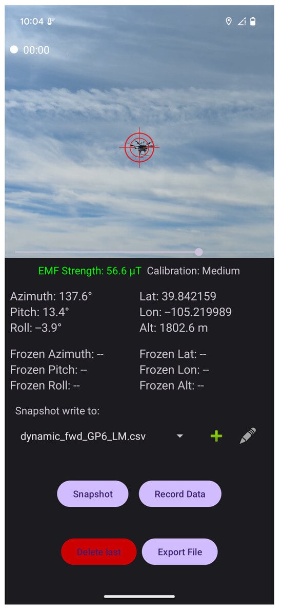
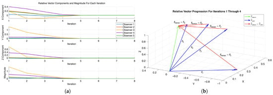
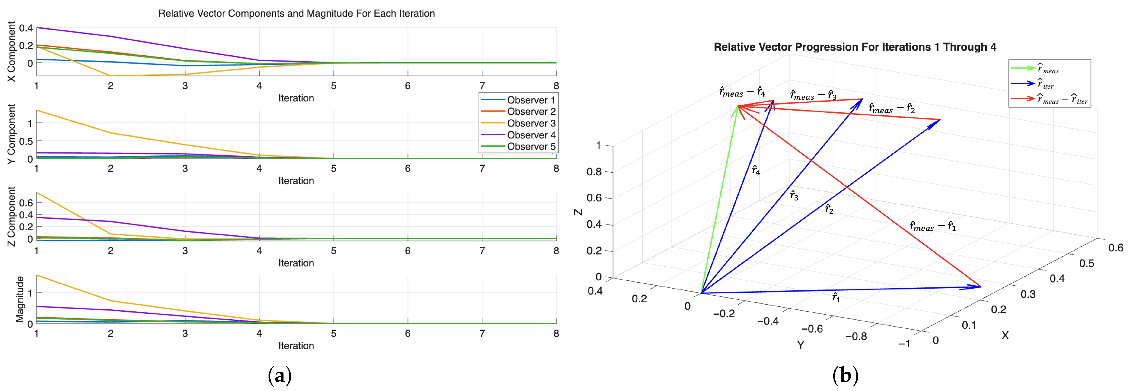
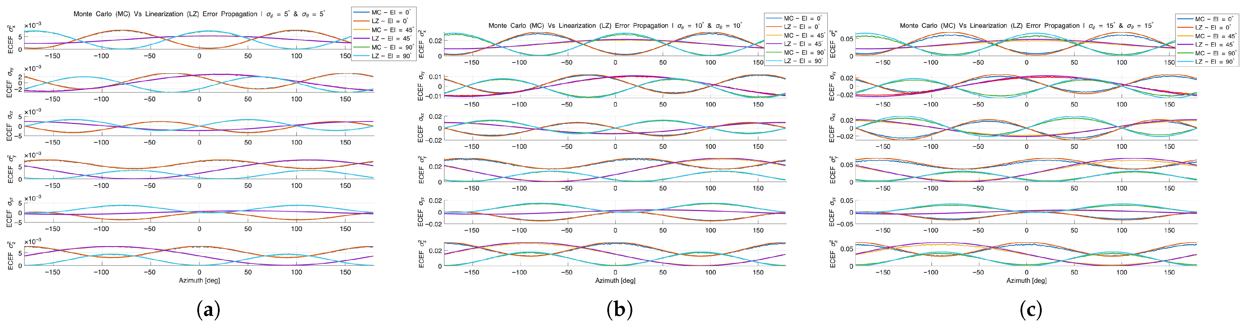
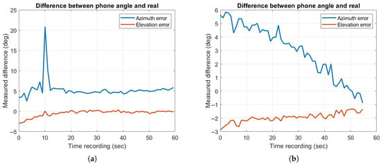
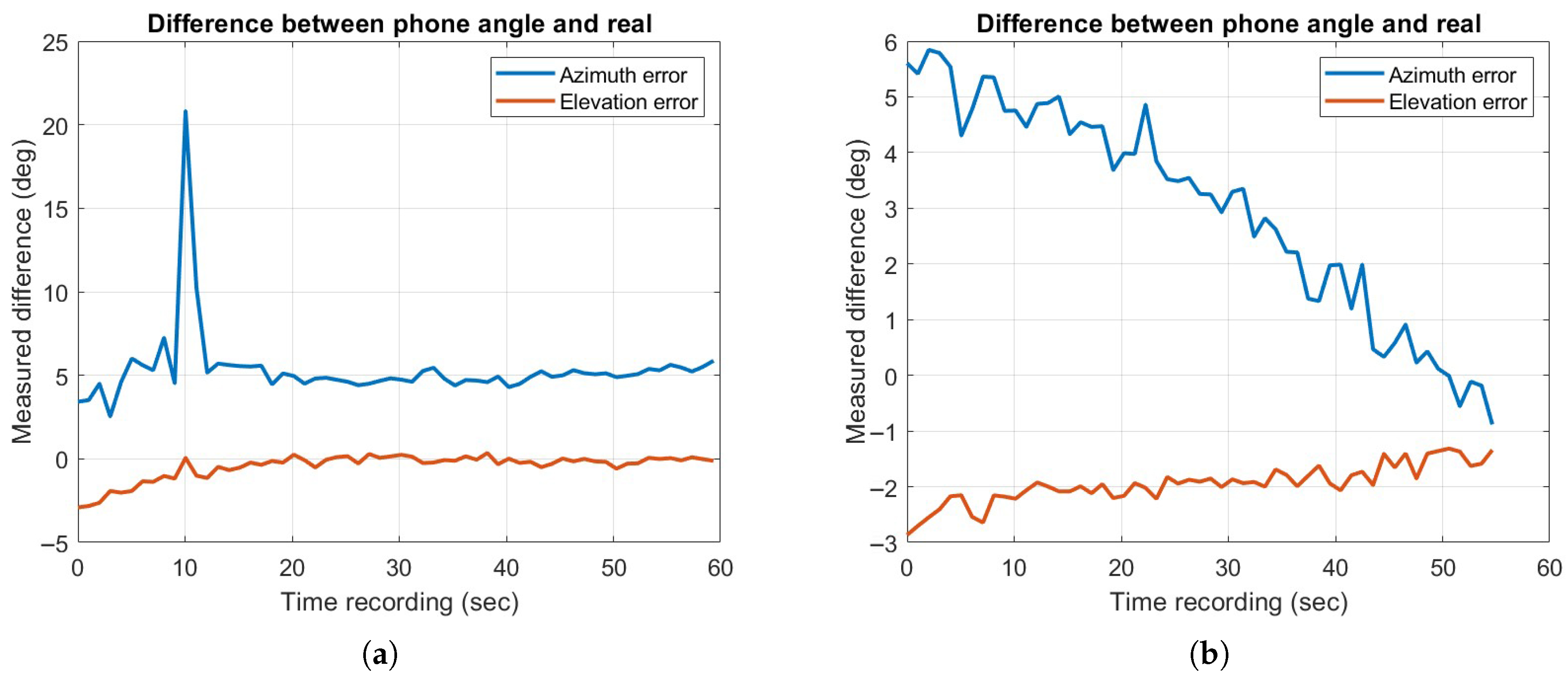
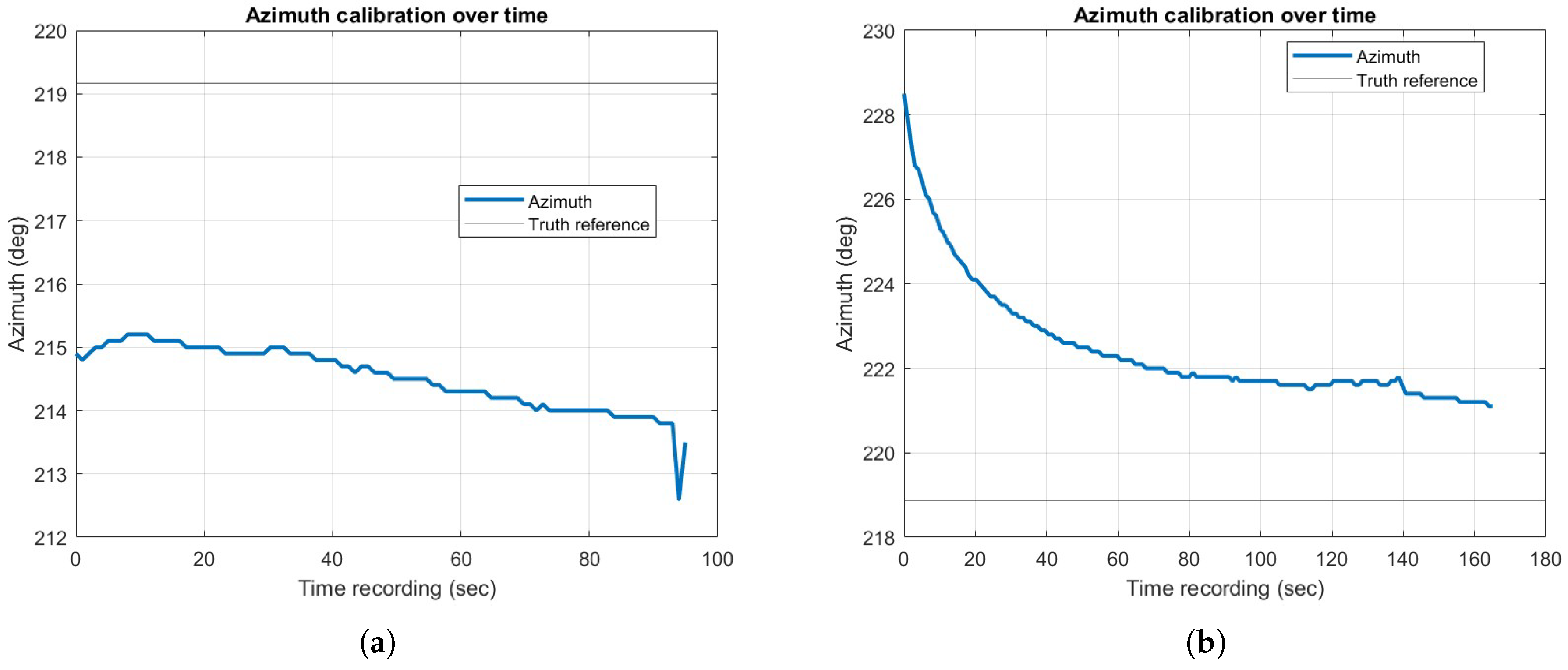
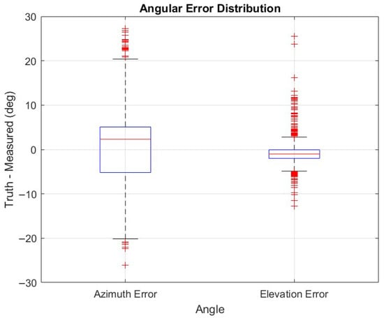
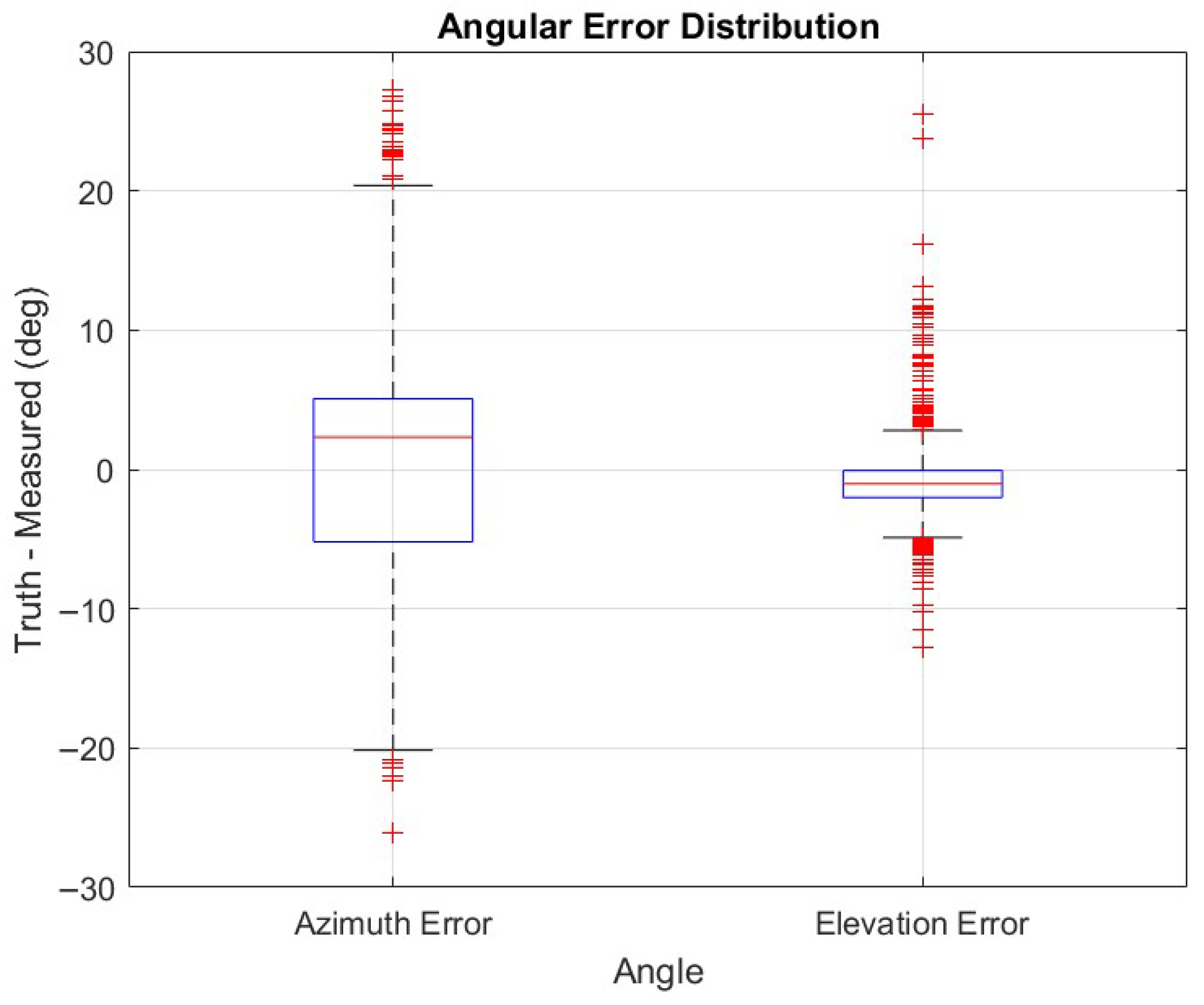
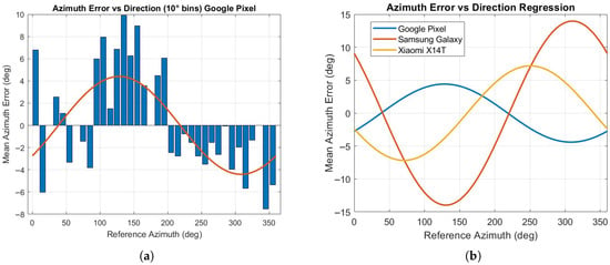
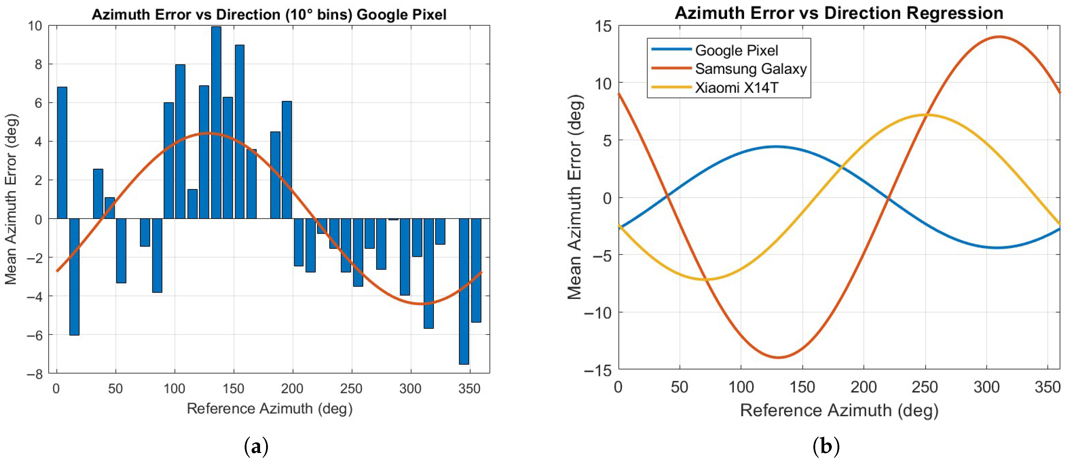
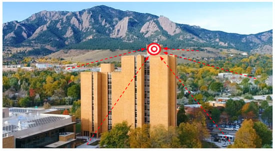
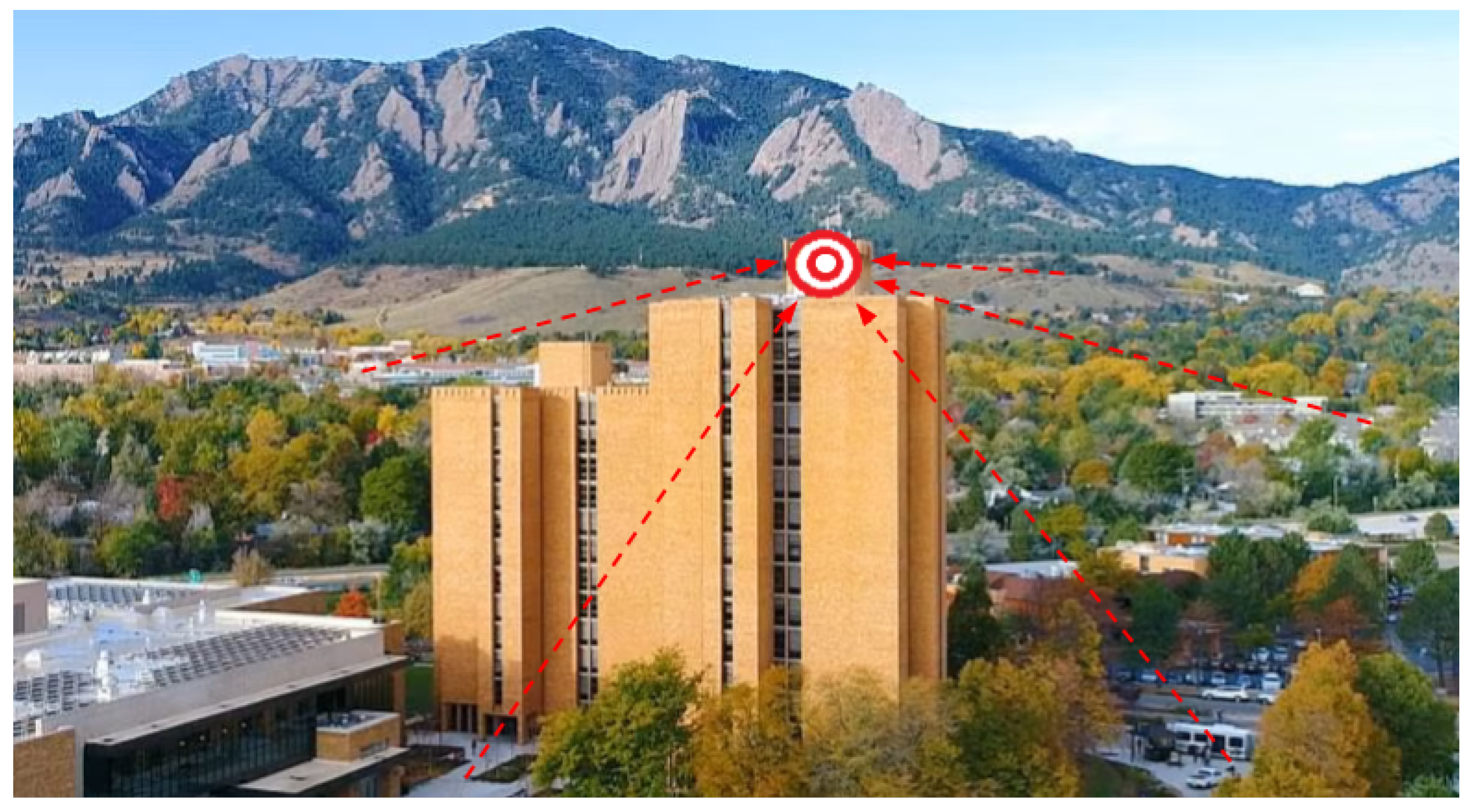
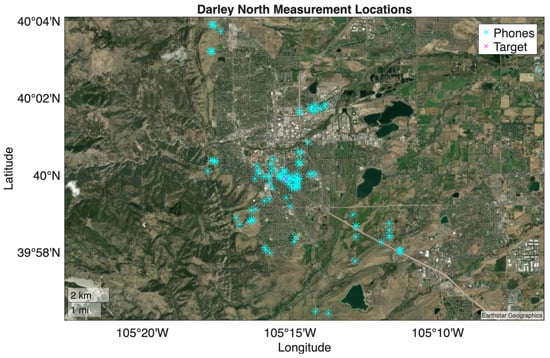
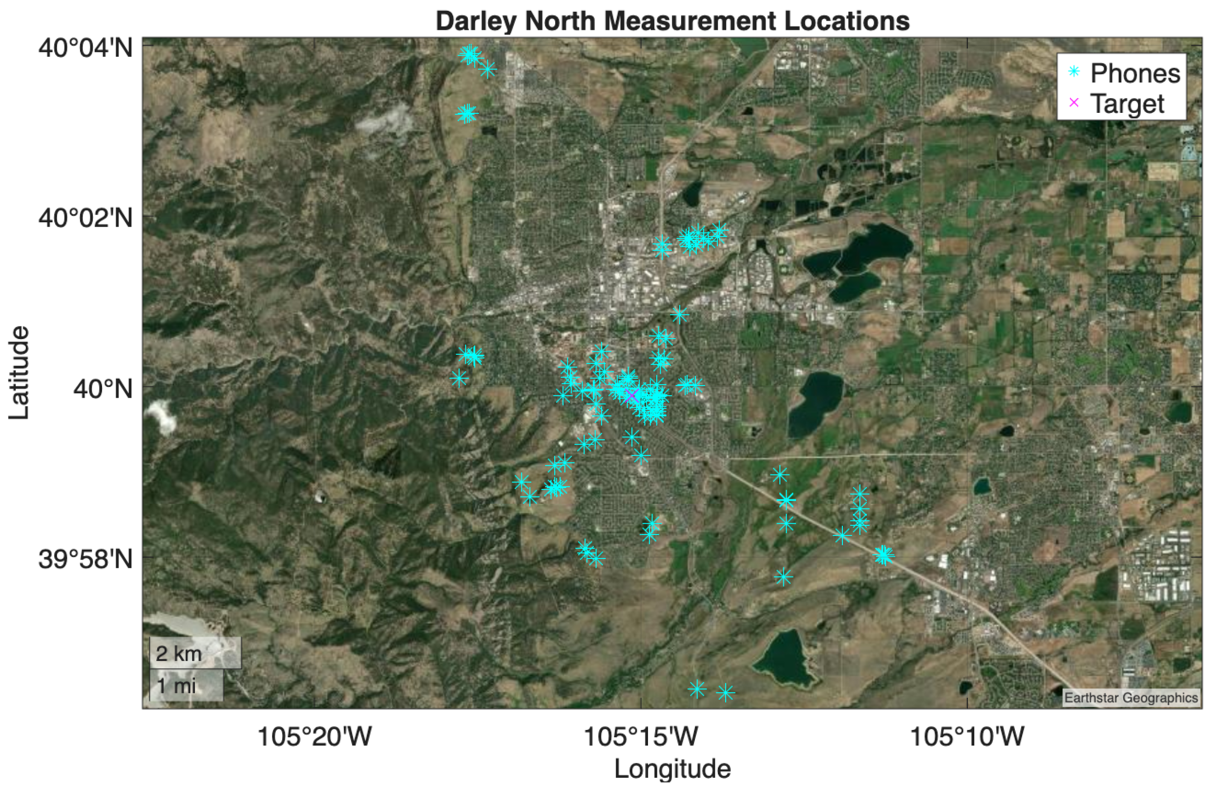
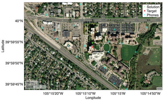
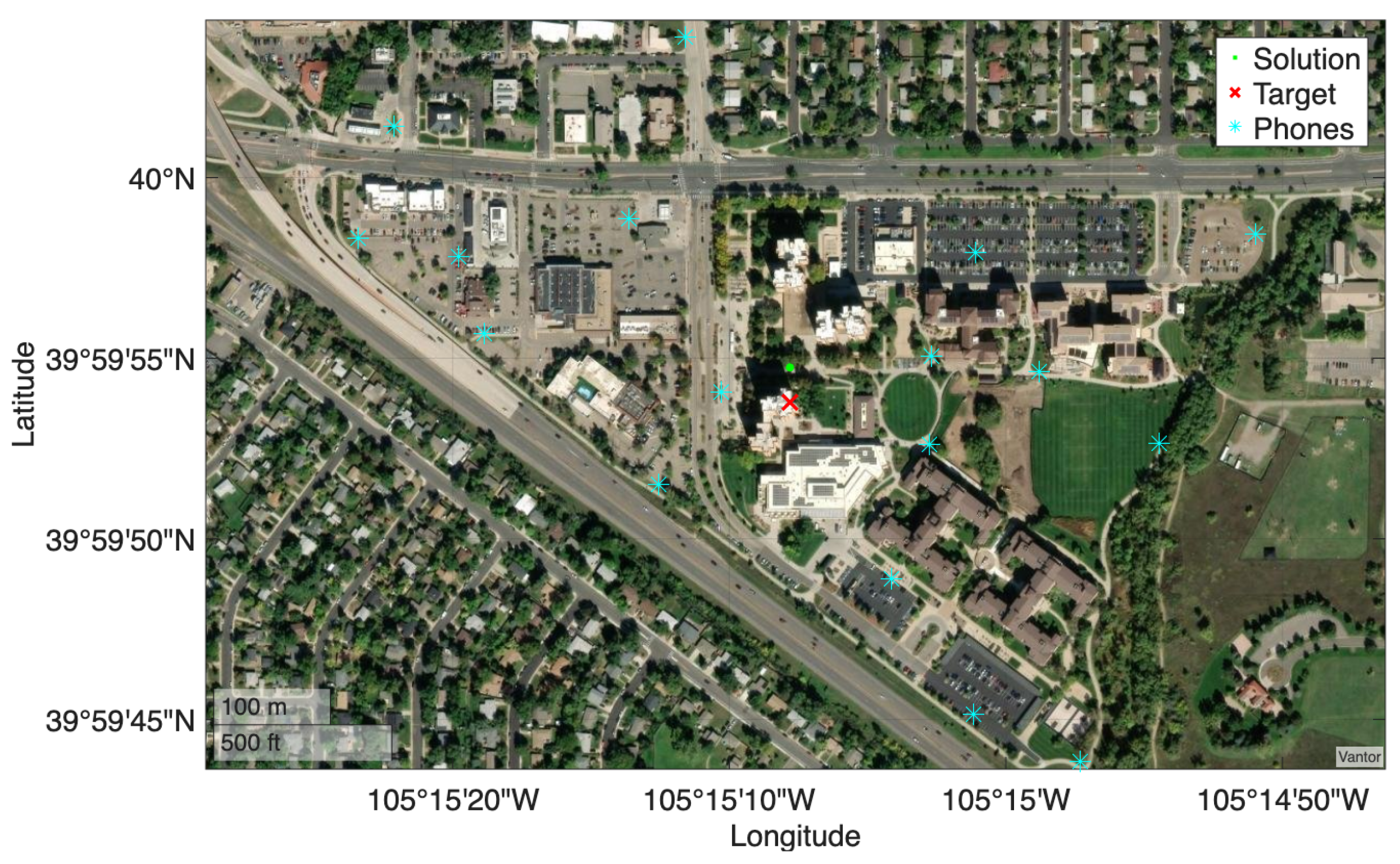
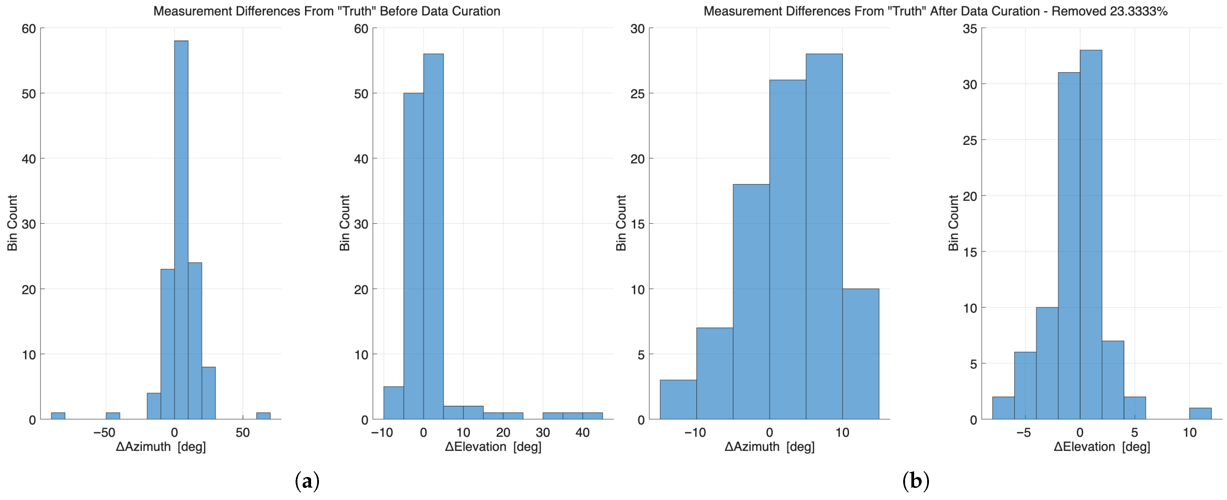
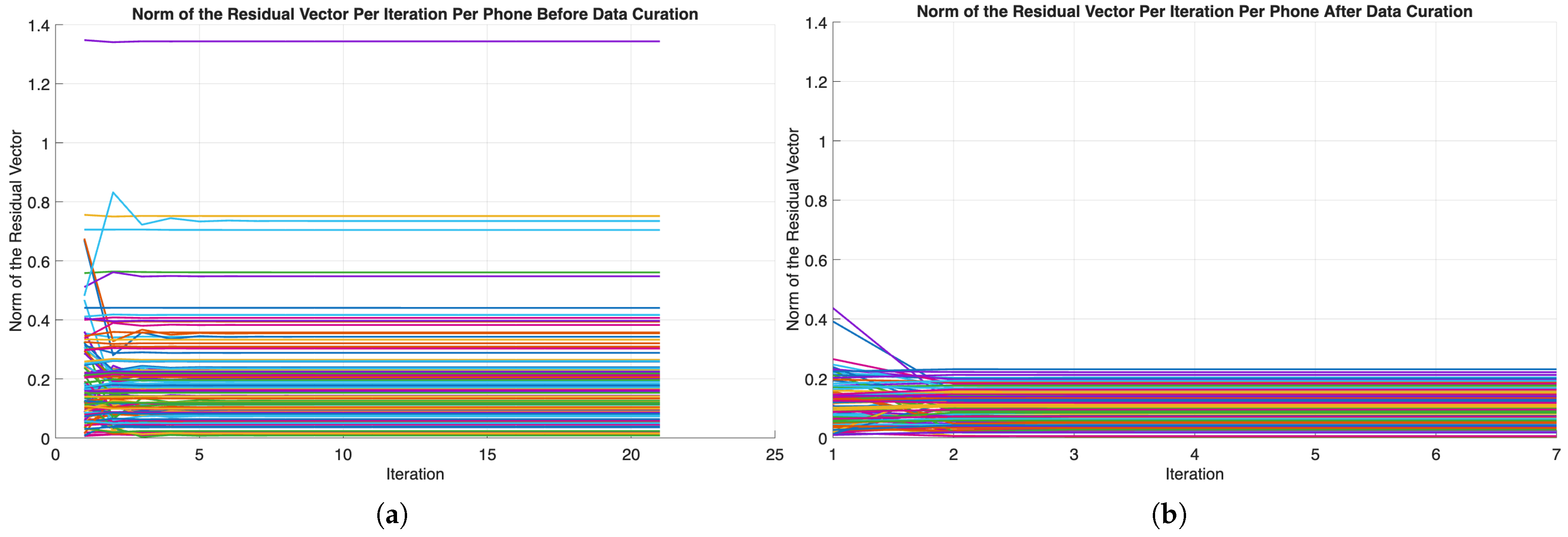
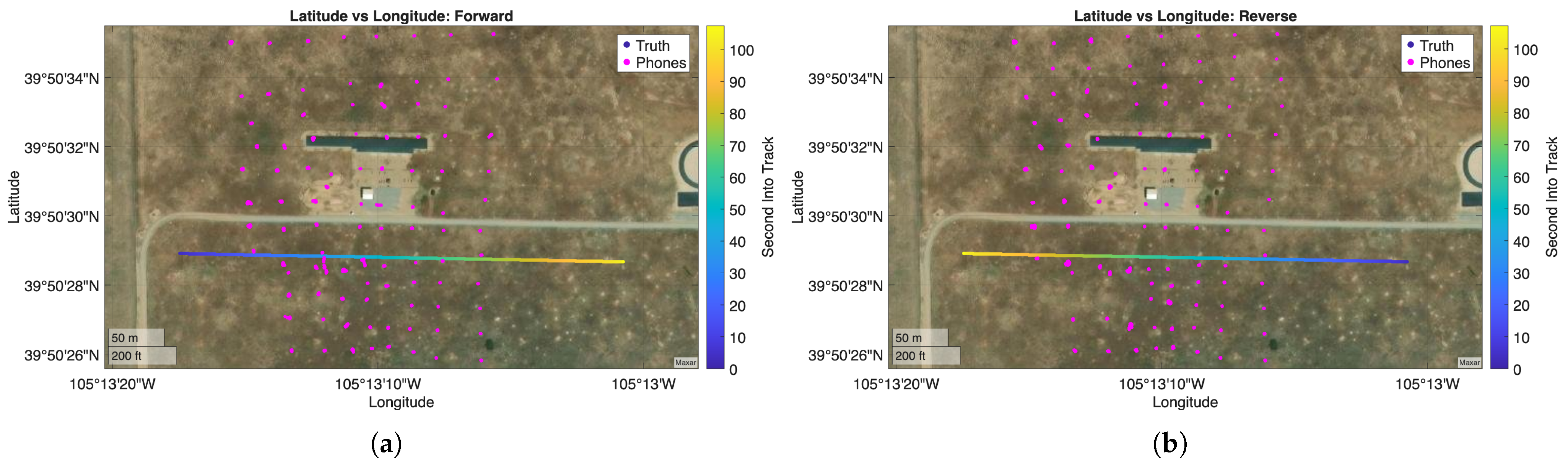
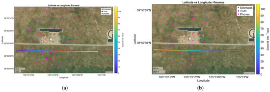
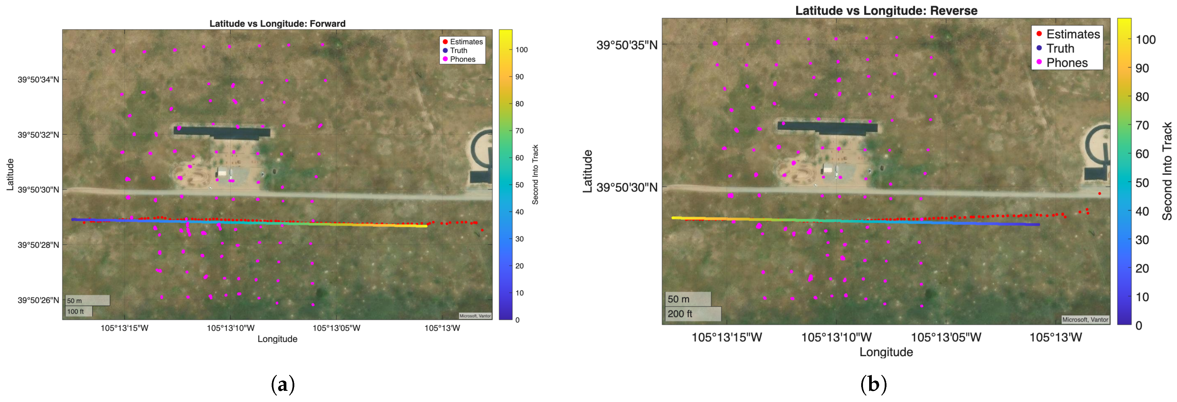
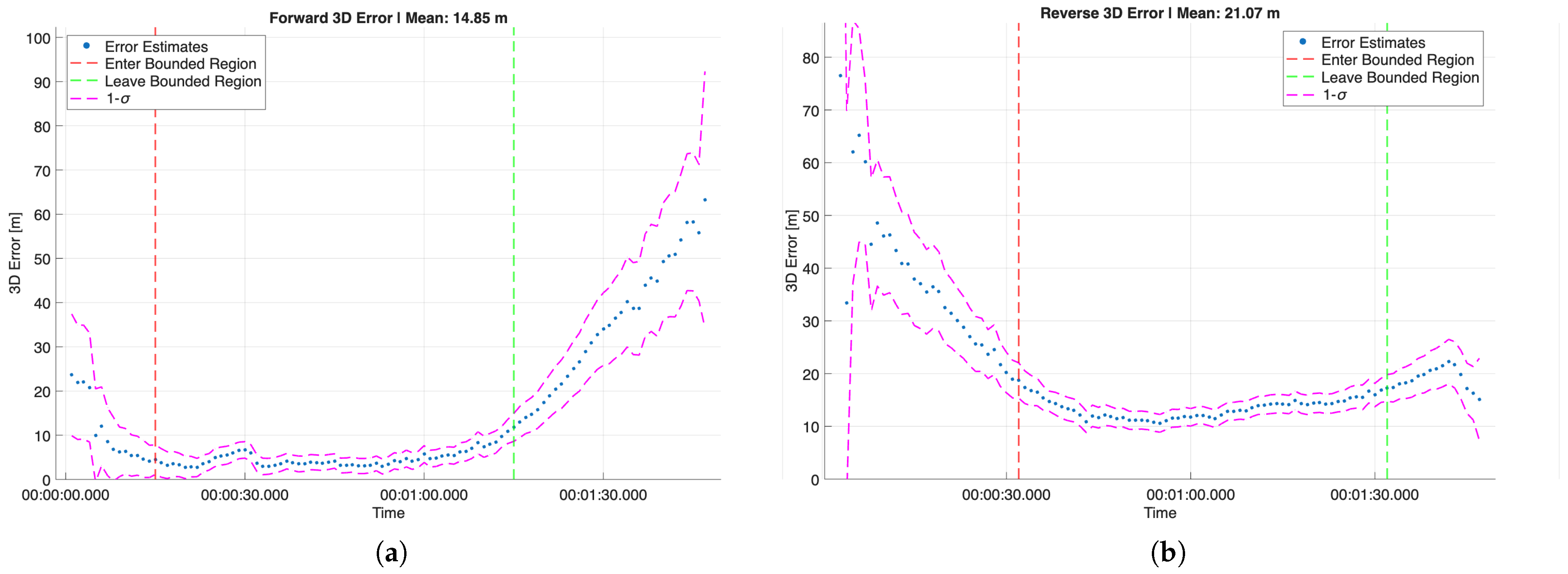
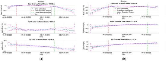
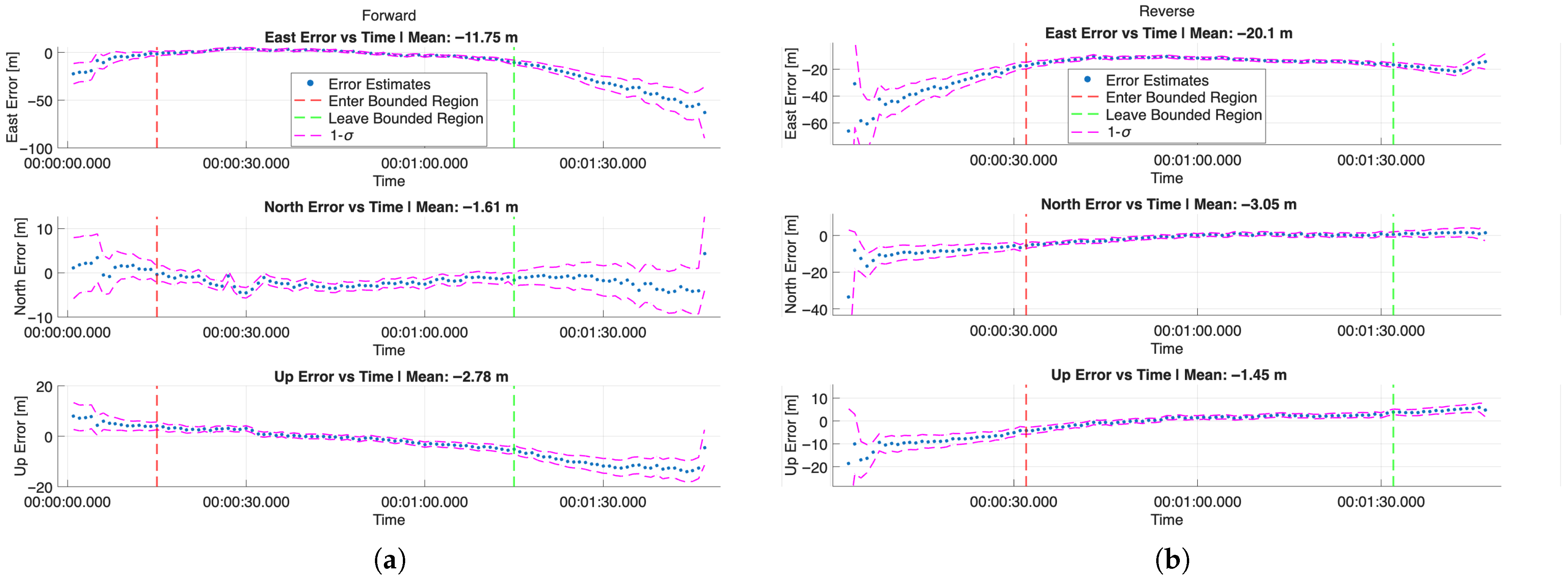
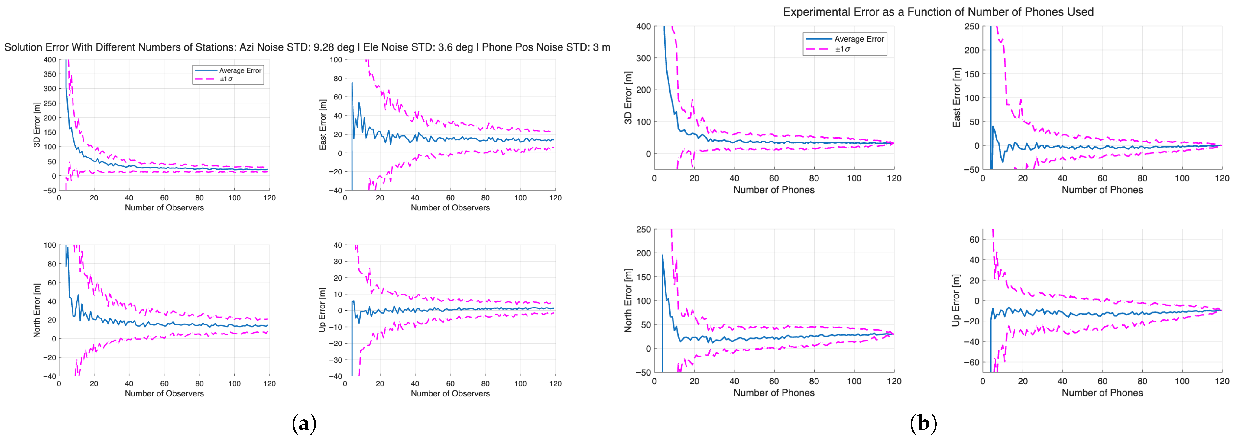
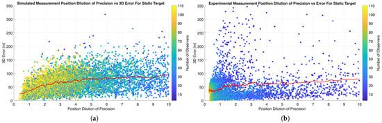
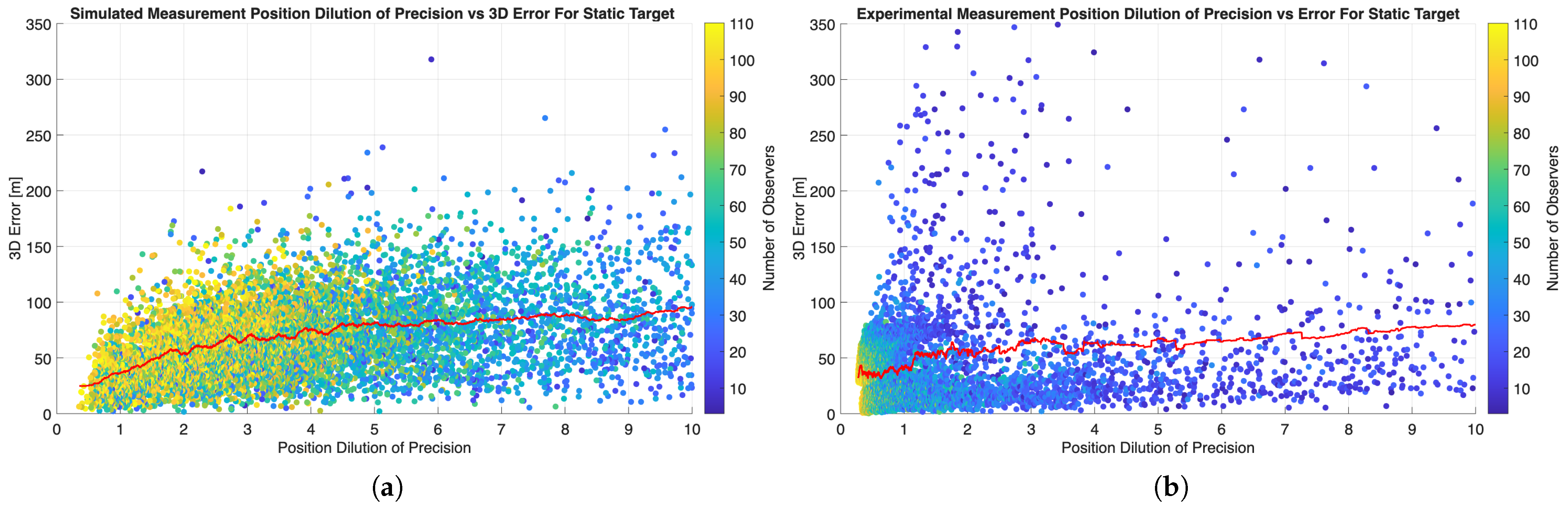
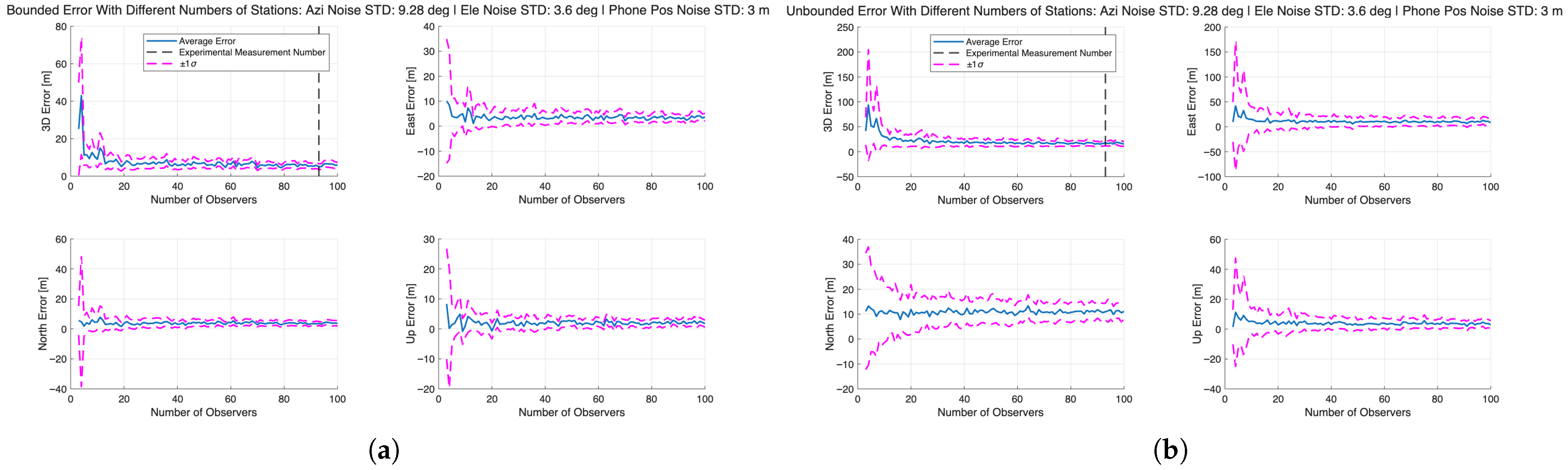

Disclaimer/Publisher’s Note: The statements, opinions and data contained in all publications are solely those of the individual author(s) and contributor(s) and not of MDPI and/or the editor(s). MDPI and/or the editor(s) disclaim responsibility for any injury to people or property resulting from any ideas, methods, instructions or products referred to in the content. |
© 2026 by the authors. Licensee MDPI, Basel, Switzerland. This article is an open access article distributed under the terms and conditions of the Creative Commons Attribution (CC BY) license.