


Highlights
What are the main findings?
- To fill the gap in existing studies that inadequately capture UAV–UGV cooperative operating characteristics and overlook real-world transport conditions, station operations, and regulatory constraints, we propose the MSUUCDSP, develop a corresponding MILP model and a Hybrid Large Neighborhood Search (HLNS) algorithm, and implement an ArcGIS-based 3D simulation for routing visualization.
- By adopting an HMM-based map-matching algorithm and big data techniques, we generate instances across four diverse scenarios. Results show that UAV–UGV cooperative delivery reduces total time cost by 17.12% and highlights significant differences between idealized assumptions and realistic conditions.
What are the implications of the main findings?
- The MILP model incorporates a novel mathematical formulation to obtain exact solutions, while the HLNS algorithm combines greedy strategies, LNS, local search, and simulated annealing to achieve high-quality solutions with an average deviation of 0.22% from the optimal. Together, they provide a scalable and efficient approach for multi-carrier delivery scheduling under complex urban constraints.
- The simulation maps optimized routes onto urban road networks, bridging the gap between optimization results and practical operations, reducing execution uncertainty, and facilitating the engineering implementation of UAV–UGV cooperative delivery.
Abstract
Urban logistics systems face growing delivery demand and complex traffic and operational constraints, which make unmanned delivery carriers, including unmanned aerial vehicles (UAVs) and unmanned ground vehicles (UGVs), a promising solution. Existing studies typically focus on a single delivery carrier type and rely on idealized assumptions, overlooking heterogeneous cooperation under multiple stations, multiple time windows, and real-world transport conditions. To address these gaps, we propose the Multi-Station UAV–UGV Cooperative Delivery Scheduling Problem with Temporally Discontinuous Service Availability (MSUUCDSP) to minimize the total travel and waiting time of UAVs and UGVs. To solve the problem, we propose a mixed-integer linear programming (MILP) model with a novel mathematical approach and a Hybrid Large Neighborhood Search (HLNS) algorithm. Additionally, we adopt a Hidden Markov Model (HMM)-based map-matching method and big data techniques to capture realistic operational characteristics. Computational experiments are conducted on various realistic instances under four diverse scenarios. Results show that UAV–UGV cooperation significantly improves efficiency, reducing total time cost by 17.12% compared with single-mode delivery, and they reveal substantial discrepancies between idealized assumptions and realistic scenarios. We further develop an ArcGIS-based simulation to support practical implementation. The findings provide valuable insights for decision-making and engineering applications for logistics operators.
1. Introduction
As e-commerce and on-demand delivery services develop rapidly, urban logistics systems are facing the dual challenges of continuously growing delivery demand and increasingly complex operating environments [1]. On the one hand, the expanding scale of delivery orders imposes higher requirements on delivery efficiency and service quality. On the other hand, practical factors such as labor shortages, traffic congestion, and urban operational constraints have gradually exposed the efficiency limitations of traditional delivery modes dominated by human-driven vehicles. In this context, unmanned delivery carriers, including unmanned aerial vehicles (UAVs) and unmanned ground vehicles (UGVs), which possess autonomous decision-making and unmanned operation capabilities, have emerged as a promising technological approach to enhancing the efficiency of urban delivery [2].
From an operational and planning perspective, the utilization of unmanned delivery carriers can be abstracted as a class of routing and scheduling problems. In particular, the efficient operation of UAVs and UGVs is commonly formulated as a routing optimization problem under a set of operational constraints [3]. Such problems are often regarded as variants of the classical Vehicle Routing Problem (VRP) introduced by Dantzig and Ramser (1959) [4]. Compared with traditional delivery modes, UAVs offer high routing flexibility and are less affected by ground traffic conditions, making them well-suited for fast, point-to-point aerial deliveries. In contrast, UGVs are constrained by urban road networks but exhibit advantages in payload capacity and endurance, which makes them more suitable for stable and continuous ground delivery tasks. In practical delivery scenarios, a single type of delivery carrier often fails to achieve an optimal balance among efficiency, cost, and feasibility. Therefore, leveraging the complementary operational characteristics of UAVs and UGVs and studying the cooperative scheduling and routing of heterogeneous unmanned delivery carriers are of significant theoretical and practical importance.
Although routing and scheduling problems for unmanned delivery have attracted increasing attention in recent years, existing studies primarily focus on a single delivery carrier type or rely on overly idealized modeling assumptions [5,6], thereby overlooking several critical operational constraints encountered in real-world conditions. First, stations are typically subject to traffic conditions, operational arrangements, and regulatory requirements. The loading, dispatching, recovery, and service activities of UAVs and UGVs are all strictly constrained by time windows. As a result, stations are generally available during specific periods, a factor that has not been explicitly considered in the literature, as they are often assumed to be available throughout the entire planning horizon [7,8]. Second, UGV movements must strictly follow the urban road network topology. Previous studies often abstract the delivery network as an idealized space, adopt Euclidean or Manhattan distance metrics [9,10], and treat vehicle speeds as constant. These simplifications deviate significantly from the complexity of real-world urban road networks. Additionally, the spatial distribution of stations and customers, as well as the advance estimation of customer demands, plays a crucial role in practical applications. Despite their importance, these parameters are typically derived from benchmark instances or randomly generated data [11,12], limiting the realism of the resulting optimization models. If such factors are not systematically incorporated, the applicability and decision-support value of optimization methods in urban logistics systems may be substantially weakened.
To address these gaps and the limitations of the prior studies, we introduce the Multi-Station UAV–UGV Cooperative Delivery Scheduling Problem with Temporally Discontinuous Service Availability (MSUUCDSP). In defining the problem, we adopt a cooperative delivery mode that integrates UAVs and UGVs, and we consider temporally discontinuous service availability in the form of station-specific multiple time windows during which stations are available for the dispatch and return of delivery carriers. These time windows reflect regulatory requirements and practical operational constraints in real-world urban logistics systems, and they build upon existing studies where depots are associated with a single service time window [13,14,15]. They are further motivated by operational requirements at both departure and return, including loading at dispatch and post-return activities such as battery recharging or swapping, and parcel handling (e.g., returns or undelivered items). Multiple time-window settings have received limited attention in the literature and remain at the customer level in VRPs [16], where only the assignment of a single vehicle to a customer’s time window needs to be considered. In contrast, our problem involves loading, departure, and return time windows and requires the simultaneous assignment of multiple vehicles’ time windows at the station level. In addition, several realistic factors are incorporated, with the distinct operating characteristics of UAVs and UGVs further captured by modeling aerial travel using Euclidean distances and ground travel based on real-world road networks and traffic conditions. Under this setting, we develop a mixed-integer linear programming (MILP) model and a Hybrid Large Neighborhood Search (HLNS) algorithm. We further integrate map matching and big data techniques to conduct extensive computational experiments, numerical analyses, and simulation studies, from which managerial insights are derived.
In this study, we need to capture all problem features to fully address this new problem in modeling and algorithm design. These constraints are not merely additive. Rather, they interact with each other, creating coordination requirements among them. Accordingly, the main contributions of this paper are as follows:
- We introduce the MSUUCDSP, a novel framework that incorporates a variety of realistic features, including multiple stations, station-specific multiple time windows, customer time windows, heterogeneous delivery carriers, half-open routing, and endurance constraints.
- We propose an MILP model and develop an HLNS algorithm that integrates greedy strategies, large neighborhood search (LNS), local search, and simulated annealing. The MILP model can be solved optimally using IBM ILOG CPLEX Optimization Studio (CPLEX) [17]. In particular, a novel mathematical approach is introduced to define the temporally discontinuous service availability mechanism.
- By adopting a Hidden Markov Model (HMM)-based map-matching method and big data techniques, we construct two types of realistic instances and design four representative scenarios, resulting in a total of 82 computational experiments. The experimental results demonstrate that the MILP model and the proposed heuristic method outperform existing methods, and that UAV–UGV cooperative delivery offers efficiency advantages while highlighting the significant differences between idealized modeling assumptions and realistic urban operating conditions.
- We further develop an urban road network simulation based on Arc Geographic Information System (ArcGIS Pro 2.6) [18] to enable realistic 3D visualization of the delivery solutions. The simulation provides detailed route guidance for UGVs and offers an intuitive and actionable decision-support tool for logistics operators and engineering applications.
The remainder of this paper is organized as follows. Section 2 reviews the related work. Section 3 presents the fundamental definitions of the MSUUCDSP, mathematical formulation, HLNS algorithm, and the HMM-based map-matching algorithm. Section 4 reports the computational experiments and simulation. Section 5 discusses the management insights, study limitations, and directions for future research. Finally, Section 6 concludes with the main ideas of this work.
2. Related Work
This section provides a brief survey of recent studies relevant to the topic. Here, we discuss related work from four perspectives: (i) UAV routing problems; (ii) their cooperative scheduling with ground vehicles; (iii) approaches for addressing these problems; and (iv) UAV–UGV delivery system applications.
2.1. UAV Routing Problem
In the literature on UAV routing problems, customer time window constraints are widely recognized as an important operational factor [19]. Time windows define the allowable time intervals during which customer service can be performed and have a significant impact on routing feasibility and solution quality. Guerriero et al. [13] formulated the UAV routing problem with soft time windows as a multi-criteria optimization model, simultaneously considering the minimization of total travel distance and the number of UAVs used, as well as the maximization of customer satisfaction. Shi et al. [20] investigated a routing problem of small UAVs for information collection with time windows, in which UAVs are allowed to be recharged at distributed platforms. To solve this problem, an improved adaptive large neighborhood search algorithm combined with simulated annealing strategies was developed. Most existing studies focused on a single time window per customer. The few existing studies addressing multiple time windows mainly emphasized customer-related characteristics in VRPs [16]. To the best of our knowledge, routing problems considering multiple time windows at UAV stations have not been reported. Furthermore, the modeling approach proposed in this paper achieves better solution performance.
Moreover, in real-world delivery scenarios, UAV operations typically involve multiple stations for dispatch and recovery, which is also directly relevant to the problem examined in our study. Stodola and Kutěj [21] proposed the multi-depot vehicle routing problem with drones, where heterogeneous trucks, each paired with a UAV, are assigned to different depots. The authors employed a metaheuristic algorithm based on ant colony optimization. Wen et al. [22] addressed the modeling complexity and multi-objective collaborative optimization challenges in multi-depot and multiple UAV delivery task planning. They proposed a bilayer planning framework that comprehensively considered resource constraints, multi-depot coordination, and the coupling characteristics of route execution. These studies highlighted the importance of considering multiple stations and the associated operational constraints in UAV routing problems.
2.2. UAV–UGV Scheduling Problem
As mentioned above, these studies primarily focus on UAVs operating independently. However, in recent years, a few researchers have begun to investigate cooperative scheduling between UAVs and ground vehicles to further improve delivery efficiency and operational flexibility. Wang et al. [23] explored a truck–drone hybrid routing problem with time-dependent road travel time and employed an iterative local search heuristic to solve it. Lu et al. [24] investigated the routing optimization problem for takeout delivery under a joint delivery scheme involving drones, occasional drivers, and riders. They developed a model with the objectives of minimizing delivery costs and maximizing overall customer satisfaction, and proposed an improved adaptive large neighborhood search algorithm to solve the problem. Han et al. [25] introduced a multi-objective vehicle routing problem with time windows and drone transportation constraints and designed an improved artificial bee colony algorithm to find high-quality solutions. In their model, vehicles were used to transport goods over the network, while drones were used to deliver parcels directly to customer locations in a vertical and timely manner. Luo et al. [26] presented a collaborative truck-drone routing problem where a truck works with multiple drones to deliver parcels, allowing service time to deviate within a given tolerance window. To solve this, they developed a hybrid multi-objective genetic optimization algorithm integrated with a Pareto local search. However, when considering the coordination with ground vehicles, the characteristics of real-world road networks become an important factor. As noted in [23,24,26], many studies calculated the distance between two nodes traveled by a ground vehicle using the Manhattan distance, which ignored the actual features of the road networks. Moreover, in most existing models, parameter values were not derived from realistic data. Overall, the study of the MSUUCDSP, which fully captures the operational characteristics of heterogeneous delivery carriers and incorporates a variety of realistic features, has not appeared in the existing literature.
2.3. Solution Methods
With respect to solution methods, the VRP and its variants have been established as strongly NP-hard [27]. Exact methods are capable of directly obtaining optimal solutions. Constructing MILP formulations and solving them with CPLEX, which is based on the branch-and-bound algorithm [28], represents an important strategy. This solution strategy has been widely adopted in the literature [29,30]. Coelho et al. [31] investigated a heterogeneous UAV fleet routing problem under limited vehicle autonomy, in which multiple charging stations and operational constraints were explicitly incorporated. The problem was formulated as an MILP model with seven objective functions to be minimized. Ribeiro et al. [32] focused on the integrated use of UAVs and mobile charging stations and formulated the problem as a VRP with synchronized networks using an MILP framework. In addition to exact methods, heuristic algorithms are also widely adopted. Although they cannot guarantee optimality, these methods are effective for large-scale problems in obtaining optimized solutions. The LNS algorithm used in this study, based on a destroy-and-repair strategy, can escape local optima and quickly find high-quality solutions [33]. Frequently applied exact and heuristic algorithms include Benders decomposition [34], column generation [35], genetic algorithm [36], local search [37], greedy algorithm [38], simulated annealing [39], variable neighborhood search (VNS) [40], and adaptive large neighborhood search (ALNS) [41]. The above studies have shown that exact and heuristic algorithms are highly effective, guiding the design of our study. The HLNS algorithm integrates multiple methods and demonstrates superior performance compared to alternative algorithms in solving the MSUUCDSP.
2.4. UAV–UGV Delivery System Applications
The delivery scheduling problem discussed above provides key technical support for the efficient operation of UAV–UGV collaborative systems. However, for practical engineering applications and deployment, additional considerations are necessary beyond planning algorithms. Munasinghe et al. [42] provided a comprehensive review of multi-UAV and multi-UGV systems, focusing on collaborative aerial and ground operations as well as the communication and coordination mechanisms that enable such cooperation. They also highlighted potential limitations and challenges, including computational constraints, communication network instability, and difficulties in adapting to dynamic environments. Kanarskyi et al. [43] noted that UAVs and UGVs are considered complex multi-state technical systems. In this context, they proposed a method for assessing the availability of monitoring systems with augmented reality–based human–machine interaction interfaces, which enable the quantitative evaluation of the overall availability and reliability of such systems. Taken together, these studies emphasized the importance of addressing safety, reliability, and operational risks in UAV–UGV delivery systems. They provide valuable guidance for the future engineering applications of the present research.
3. Problem Description and Methods
This study proposes the development of the MSUUCDSP, including an MILP model and an HLNS algorithm, with the aim of minimizing the total travel and waiting time of UAVs and UGVs. In particular, the study employs an HMM-based map-matching approach to capture the transport characteristics of unmanned delivery carriers in practical delivery scenarios.
3.1. Problem Statement
The following provides a formal description of the MSUUCDSP:
- The delivery network is composed of a set of stations and a set of customers. Each station stores goods destined for customers and serves as a dispatch and return node for unmanned delivery carriers. The geographic locations of all stations and customers are known in advance. Delivery carriers may start their delivery missions from one station and terminate at the same or a different station, with a half-open routing scheme.
- The total number of available UAVs and UGVs in the delivery network is limited, while each station is assumed able to dispatch carriers as long as the overall fleet size constraint is satisfied. The payload capacity and endurance of each unmanned delivery carrier, as well as the loading speed at stations, are known and fixed.
- The demand of each customer is known and indivisible. Service to each customer is provided by one unmanned delivery carrier. Each customer may be served by either a UAV or a UGV, and the selection of the delivery carrier type is treated as a decision variable in the optimization process. The stations are assumed to have sufficient inventory to satisfy all customer demands.
- Due to operational and regulatory constraints, the temporally discontinuous service availability of stations is implemented as a service mechanism within specific time periods. Each station is associated with multiple time windows during which loading, dispatching, and recovery operations are allowed. Unmanned delivery carriers can only be loaded and dispatched when the corresponding station is available. After completing customer service, the delivery carriers must return to a station within its availability time window, and early arrival with waiting is prohibited.
- Customer service time windows define the allowable service intervals. Unmanned delivery carriers may arrive earlier than the time window but must initiate service within the specified interval. Late arrivals beyond the customer time window are not permitted.
- Real-world delivery conditions are considered to distinguish different transport characteristics of unmanned delivery carriers. UAVs are assumed to travel directly between nodes, and their travel distances are calculated based on Euclidean distances. In contrast, UGVs are constrained by the urban road networks, and their delivery routing must follow the actual road topology.
Figure 1 illustrates an example of the MSUUCDSP, which involves three stations and eight customers. Each station has two time windows. A UAV from Station 1 carries the goods for Customers 1, 3, and 4, provides service within the customer time windows, and returns to the same station after completing the delivery. Loading, dispatching, and recovery operations must be performed within the service availability period of Station 1. The remaining customers are served by UGVs A and B, which also operate within the customer and station time windows. UGV B follows a half-open routing scheme and returns to Station 3 after completing the service. It should be noted that UAVs travel along straight-line routes, whereas UGVs are constrained by the urban road networks throughout the entire delivery process. The temporally discontinuous service availability of stations means that services can only be provided within the gray-shaded boxes. These two characteristics also represent key innovations of the MSUUCDSP.
Figure 1.
Example of the MSUUCDSP.
3.2. Mathematical Formulation
We develop an MILP model to represent the MSUUCDSP. The proposed mathematical model can be directly solved using CPLEX 12.9 based on branch-and-bound, which is capable of providing exact solutions. The model mainly consists of parameters and decision variables, the objective function, and constraints. Among these, the constraints are organized into six subsections: routing constraints, assignment constraints, temporally discontinuous service availability constraints, customer time window and time continuity constraints, unmanned delivery carrier use constraints, and other constraints. The key factors in the construction of the model are threefold: (i) establishing the relationship between UAVs and UGVs based on the objective function, and distinguishing the two types of carriers through time continuity constraints and unmanned delivery carrier use constraints; (ii) formulating the relationships among customers, stations, and carriers using assignment constraints; and (iii) capturing the multi-time-window characteristics of stations by employing temporally discontinuous service availability constraints.
To ensure consistency and clarity, the related symbols are kept uniform and definitions for all symbols are provided in Table 1. The MSUUCDSP is formulated as follows.
Table 1.
Parameters and variables.
The objective function (1) minimizes the total time, comprising three components: the travel time of UAVs and UGVs, and the waiting time incurred by UAVs and UGVs at customer nodes. The main objective of this study is to minimize the total system time. Therefore, the objective function treats these terms equally. This assumption is also consistent with some existing VRPs and UAV–UGV scheduling problems [19,20,44].
- Routing constraints
Constraint (2) ensures that the numbers of departures from and returns to stations are balanced for each unmanned delivery carrier. The departure and the return stations may be the same or different.
Constraint (3) guarantees that the number of arrivals at each customer equals the number of departures, and that each customer is served exactly once.
- Assignment constraints
Constraint (4) specifies that customer demands must be supplied by stations, meaning that all customer demands are fulfilled by the inventory stored at the stations.
Constraint (5) indicates whether a customer node is served by an unmanned delivery carrier.
Constraints (6)–(7) describe whether the demand of a customer is delivered by an unmanned delivery carrier departing from a station, thereby defining the service relationship among stations, unmanned delivery carriers, and customers.
Constraints (8)–(9) ensure that if an unmanned delivery carrier assigned to a station is utilized, it must depart from that station to perform delivery services.
- Temporally discontinuous service availability constraints
Constraints (10)–(11) specify that an unmanned delivery carrier can start loading goods only after the opening of a time window at the corresponding station.
Constraints (12)–(13) ensure that an unmanned delivery carrier starts loading goods before the closing of the corresponding time window at the station.
Constraints (14)–(21) are used to determine the specific time window during which an unmanned delivery carrier starts loading goods at the station.
Constraints (22)–(23) ensure that if an unmanned delivery carrier is utilized, it must load goods within the time window of the station.
Constraint (24) ensures that each unmanned delivery carrier completes the loading operation within the station time window and then departs to serve customers.
Constraints (25)–(26) describe the continuity between the loading start time and the departure time of the unmanned delivery carrier. Together with Constraint (24), they ensure that unmanned delivery carriers can only be loaded and dispatched when the corresponding station is available.
Constraints (27)–(28) ensure that the unmanned delivery carrier returns to the station after the opening of the corresponding time window.
Constraints (29)–(30) ensure that the unmanned delivery carrier returns to the station before the closing of the corresponding time window.
Constraints (31)–(38) are used to determine the specific time window during which an unmanned delivery carrier returns to a station after completing delivery services.
Constraints (39)–(40) ensure that if an unmanned delivery carrier is utilized, it must return within the time window of the station.
- Customer time window and time continuity constraints
Constraint (41) imposes the time window constraint when an unmanned delivery carrier serves a customer.
Constraints (42)–(45) ensure the time continuity of UAVs and UGVs from stations to customers.
Constraints (46)–(49) ensure the time continuity of UAVs and UGVs between customers.
- Unmanned delivery carrier use constraints
Constraint (50) imposes the payload capacity constraints of each unmanned delivery carrier.
Constraints (51)–(52) enforce the endurance requirements of UAVs and UGVs for delivery services.
Constraints (53)–(54) specify the limits on the number of UAVs and UGVs allowed in the entire delivery network.
- Other constraints
Constraints (55)–(59) define the range for each variable.
For the proposed MILP model, the key challenge lies in characterizing temporally discontinuous service availability, namely the representation of station-specific multiple time windows. Due to the involvement of discontinuous time intervals and their selection, a direct linearization of this feature is nontrivial. To address this issue, we develop a novel mathematical formulation by introducing several auxiliary decision variables, including , , , and , which are designed to represent and establish logical relationships for the primary decision variables and . The detailed modeling structure is presented in Constraints (14)–(21) and (31)–(38).
A numerical illustration is provided here to further demonstrate the role of the auxiliary variables. For example, suppose that unmanned carrier k departs from station m to provide service, and the station’s time windows are [10,12] and [14,16]. Then, and are 10 and 12, respectively, while and are 14 and 16, respectively. If the loading start time of the carrier k is 11, then , , and take the value 1, while takes the value 0. Therefore, , indicating that unmanned carrier k is loaded during the first time window.
It is possible to directly adopt the approach used in existing studies for customers’ multiple time windows—without introducing auxiliary variables—by replacing Constraints (14)–(21) and (31)–(38) with Constraints (60)–(63) [16,45]. Experiments show that our proposed approach, which introduces auxiliary variables, achieves better computational performance. This will be further explained in Section 4.2.1.
Additionally, in practical enterprise operations, the deployment of unmanned delivery carriers is typically confined to limited service areas due to traffic conditions and operational scale considerations, rather than large-scale rollouts. Therefore, for medium-scale scenarios such as community-level distribution, directly solving the MILP model using exact methods can generally satisfy operational requirements. However, as future applications move toward larger-scale deployments, the problem size will increase significantly. Accordingly, the following section introduces a heuristic algorithm designed to efficiently solve larger-scale MSUUCDSP instances, which also serves to validate the accuracy of the MILP solutions.
3.3. Hybrid Large Neighborhood Search Algorithm
To address the MSUUCDSP, we propose an HLNS algorithm. The specific operational procedure of the proposed algorithm is illustrated in Figure 2, and the corresponding pseudocode is provided in Algorithm 1.
Figure 2.
Flowchart of the HLNS algorithm designed for the MSUUCDSP.
The HLNS algorithm integrates four main modules: initial solution construction, LNS [33], local search [37], and a simulated annealing strategy [39]. The LNS framework, originally proposed by Shaw [46], aims to iteratively improve an initial solution by exploring large-scale neighborhoods and relies on destroy and repair operators. The destroy operator extracts a subset of elements from the current solution according to predefined rules, whereas the removed elements are reinserted into the partially destroyed solution by the repair operator, thereby reconstructing a complete solution. Due to its strong exploration capability and flexibility, LNS has been widely and successfully applied to a variety of combinatorial optimization problems [47].
A greedy heuristic is first employed to generate an initial solution in this study [38], which serves as the starting point of the HLNS procedure. Subsequently, a random removal operator is employed to remove a subset of customers [48], and a greedy insertion operator is used to reinsert these customers into the routes [49], thereby generating a new solution. To further enhance the exploration of the search space, seven local search neighborhood structures are designed to intensify the search process. Finally, the simulated annealing acceptance criterion is adopted to determine whether the newly generated solution should be accepted. Inferior solutions are accepted with a certain probability, which helps the algorithm escape from local optima.
| Algorithm 1: HLNS algorithm | |
| Input: instance data | |
| 1 | Generate initial solution X0 |
| 2 | Xcurrent = X0 |
| 3 | Xbest = X0 |
| 4 | for iter = 1 to maximum number of iterations do |
| 5 | Xnew = Repair (Destroy (Xcurrent)) |
| 6 | Xnew = Local Search (Xnew) |
| 7 | if f(Xnew) < f(Xbest) then |
| 8 | Xbest = Xnew |
| 9 | Xcurrent = Xnew |
| 10 | else |
| 11 | if acceptance criterion is satisfied then |
| 12 | Xcurrent = Xnew |
| 13 | end if |
| 14 | end if |
| 15 | end for |
| 16 | return Xbest |
3.3.1. Initial Solution
The initial solution is generated using a greedy strategy, with the procedure detailed as follows and illustrated in Figure 3.
Figure 3.
Flowchart of the procedure for generating the initial solution for the MSUUCDSP.
Step 1: Construct the UAV assignment sets. All customers are initially assumed to be served by UAVs, and UAV delivery routes are given priority in construction. For each customer , the station that minimizes travel time is selected, resulting in the customer assignment set for each station.
Step 2: Generate the UAV routes. UAV routes are generated for each station based on . The loading start time for each UAV is set to which is the earliest opening time of the first time window of the corresponding station. Customers are then sequentially added to the route according to the principle of minimum travel time from the current node, while satisfying customer time windows, payload capacity, endurance, and station time window constraints. During route construction, the loading start time is dynamically adjusted as customers are added. Once any constraint is violated, customer insertion stops and the current route is finalized. The final return station is determined according to the greedy criterion. The station that minimizes travel time from the route’s final customer and satisfies the station time windows is selected as the return node. UAV routes are constructed continuously following this procedure until the maximum number of UAVs is reached or no more customers can be added due to constraint violations.
Step 3: Generate the UGV routes. UGVs serve customers previously not successfully assigned, forming a new customer assignment set . The same construction strategy is then applied for UGV routes.
Step 4: Adjust the waiting time. After each route is constructed, the maximum allowable adjustment time for the route is calculated, and the loading start time is further adjusted within feasible limits to reduce waiting time.
3.3.2. Large Neighborhood Search and Local Search
The LNS phase adopts random removal and greedy insertion operators. First, a certain proportion of customers are randomly selected and removed from all current routes. Then, based on a greedy strategy, the selected customers are reinserted into their best feasible positions and routes, that is, the insertion that results in the minimum increment in the objective function is chosen. It should be noted that routing adjustments may involve reconsiderations regarding station time windows for loading, dispatching, and recovery. In addition, since there are two types of routes, including UAV and UGV routes, each insertion operation must not only verify whether the modified route itself satisfies all constraints, but also ensure that the entire delivery network complies with the limited number of unmanned delivery carriers. The corresponding return station is also updated accordingly.
In the local search phase, we design seven neighborhood structures and adopt a parallel framework to further enhance the solution quality. The neighborhood structures include node relocation, insertion, swap, and route creation. Specifically, the relocation operation involves repositioning a node within the same route. The insertion and swap operations are performed between two different routes. For the insertion operation, either one node or a sequence of two or three nodes is transferred from one route to a different route. The swap operation consists of exchanging one node from one route with one node or two consecutive nodes from another route. The route creation operation refers to selecting a new node to construct a new route, where we prioritize constructing a UAV route. Overall, among the seven neighborhood structures, node relocation and route creation each represent one operator. The insertion operator is classified into three types, denoted as insertion (φ,0), and we adopt insertion (1,0), insertion (2,0), and insertion (3,0). The swap operator is classified into two types, denoted as swap (φ1,φ2), and we adopt swap (1,1) and swap (1,2). Additionally, throughout the entire optimization process, all operations should satisfy the same constraints as those applied in the LNS phase.
3.3.3. Simulated Annealing Criterion
After generating a new solution , the algorithm does not necessarily accept it, but determines acceptance according to the simulated annealing criterion. This mechanism is inspired by the analogy between combinatorial optimization and physical annealing, which allows the algorithm to escape from local optima while balancing exploration and exploitation. Specifically, if is better than the best-known solution , it is accepted directly. Otherwise, it is accepted with a probability , which is given by Equation (64), where denotes the current temperature. As the iterations proceed, the system temperature gradually decreases following an exponential cooling schedule described in Equation (65), where is the cooling coefficient. A random number is generated from a uniform distribution , and is accepted if .
3.4. HMM-Based Map-Matching Approach
In the MSUUCDSP, the UGVs’ movement is constrained by the urban road networks, unlike UAVs, which can travel in a straight line. Therefore, to accurately model UGV travel distance and time, map-matching techniques must be applied to project the UGVs’ routes onto the real-world road networks.
We adopt a Hidden Markov Model (HMM)-based map-matching approach [50], which treats the road segment sequence as hidden states and the estimated UGV positions as observations. Let denote the road network graph, where N is the set of nodes and E is the set of directed edges (road segments). For a sequence of planned UGV waypoints , where each is a coordinate in Euclidean space, we aim to find the most probable road segment sequence with .
The HMM is defined as follows: Observation probability represents the likelihood that a UGV located on road segment is observed at position . Assuming Gaussian measurement noise, this probability is given by Equation (66), where ) is the Euclidean distance from to , and is the standard deviation of GPS errors.
The transition probability , which models the plausibility of moving from segment at to segment at , is based on network connectivity and travel consistency, as given by Equation (67). is the shortest path distance in G, is the Euclidean distance, is a scaling parameter, and is an indicator function that equals 1 if and are connected in G, and 0 otherwise.
The optimal matching sequence is obtained via the Viterbi algorithm [51], which maximizes the following:
To improve computational efficiency in large-scale networks, we restrict candidate segments for each to those within a radius . Considering the urban road networks and typical GPS error characteristics, we set [52], which effectively balances coverage and computational cost.
The matched road sequence is then used to compute the UGV’s actual travel distance and time, considering road segment lengths and speed limits. This ensures that UGV routing constraints are realistically incorporated into the optimization model.
4. Computational Experiments
Our computational study consisted of two types of experiments to evaluate the performance of the MILP model and the HLNS algorithm. We also developed an urban road network simulation based on ArcGIS to enable realistic 3D visualization of the delivery solutions.
4.1. Test Instances and Scenario Settings
The first type of computational experiments involved 16 realistic instances and four research scenarios, resulting in a total of 64 experiments to comprehensively evaluate the proposed approach. The second type of experiments involved nine groups of larger-scale instances, comprising a total of 18 instances under two selected scenarios. The MSUUCDSP model was solved with CPLEX 12.9, and the HLNS algorithm was implemented using C++, both on a computational platform featuring an Intel Core i7 Quad-Core processor (3.60 GHz) and 16 GB of memory. CPLEX was executed with default parameter settings, and the duration of each computation was restricted to a maximum of 5400 s. For the HLNS algorithm, the destruction rate, the maximum number of outer iterations, and the number of inner local search iterations were set to 0.15, 1000, and 20, respectively. The cooling coefficient was fixed at 0.95, and the initial temperature was dynamically adjusted according to the scale of the instances. The urban simulation environment was established in ArcGIS, where Python 3.11 scripts [53] were employed to control ArcGIS and carry out the simulation tasks.
The study focused on the core urban area of Chongqing, China, which was selected to generate realistic instances. In this process, we employed a combination of real-world data, simulated and derived data, as well as empirical and assumed parameters.
The real-world data used in this study included the following. We obtained candidate station locations by using online map APIs (the API of online maps is available at https://lbs.amap.com/). Then, mobile signaling data were obtained from China Telecom in Chongqing under a data usage agreement, providing anonymized aggregate population distribution within the study area.
Combined with these datasets and other information, we calculated the customer demand and travel time between nodes, which were considered simulated and derived data. (i) First, by combining mobile signaling data preprocessing techniques with the Voronoi diagram method [54], we identified base stations from mobile signaling data as customer locations and determined their service areas along with the corresponding population sizes. (ii) Second, a weighted prediction model was used to estimate the potential demand of customers [55], serving as a substitute for actual order data in the experimental calculations. Specifically, population size, traffic conditions, and points of interest representing logistics demand (e.g., commercial and office facilities) were selected as evaluation indicators, and the corresponding indicator values were calculated based on the service areas delineated for each customer. Subsequently, the analytic hierarchy process was applied to determine the weights of the three indicators [56], followed by a consistency check, resulting in a comprehensive weight coefficient for each customer. Finally, the total initial demand was allocated according to the weight coefficients of each customer to obtain the predicted demand. (iii) Third, we applied the proposed map-matching techniques with the Dijkstra algorithm to compute travel time between nodes in the road networks [57].
In addition, drawing on empirical insights from urban logistics operations and previous studies, we determined the values of the remaining parameters in the MSUUCDSP. Key parameters such as endurance time, payload capacity, and travel speed were set with reference to existing literature [23,55,58], while the other parameters were assumed based on experience. More specifically, UAV and UGV payload capacities were set to 30 kg and 150 kg, respectively, and their endurance was set to 0.5 h for UAVs and 8 h for UGVs. The loading speed at stations was 1000 kg/h, the UAV travel speed was 50 km/h, and each station had 2–3 time windows. The maximum numbers of UAVs and UGVs were each set between 2 and 12.
In general, the majority of the data originate from real or derived sources, with a portion based on modeling assumptions, and these data reasonably represent real-world urban logistics systems. As an example, we selected the Lijia area to illustrate the relevant information, as shown in Figure 4, where the dotted line represents the boundary of the area. In Figure 4c, the colored frames indicate the service areas associated with each customer. In Figure 4b,d, the color gradient from green to red indicates increasing population size and customer demand, with red representing the highest level and green the lowest level. For Figure 4b, the color represents the population ranges within the service areas of customers. Specifically, green, yellow, orange, and red correspond to population ranges of 200–500, 500–800, 800–1000, and more than 1000 people, respectively. For Figure 4d, the color reflects the relative levels of customer demand, measured in kilograms (kg). Based on our calculations, the estimated demand intervals corresponding to green, yellow, orange, and red are 10–30 kg, 30–50 kg, 50–80 kg, and more than 80 kg, respectively.
Figure 4.
Example of the Lijia area. (a) Node distribution. (b) Population sizes based on mobile signaling data. (c) Customer service areas. (d) Customer demand forecast.
Four research scenarios were considered, namely the working-day scenario, non-working-day scenario, idealized scenario, and pure-UGV scenario. The differences among these scenarios mainly lay in the delivery mode and the travel time calculation scheme for UGVs, as detailed below. (1) In terms of the delivery mode, the first three scenarios adopted a collaborative delivery strategy involving UAVs and UGVs. In contrast, the pure-UGV scenario allowed only UGVs to perform deliveries, which was designed to evaluate the performance advantages of the collaborative delivery mechanism. (2) Regarding travel time settings, the idealized scenario followed the common assumptions adopted in existing studies, where the travel distance between nodes for UGVs was measured using Euclidean distance, and vehicles were assumed to move at a constant speed. In the remaining scenarios, UGVs traveled along the real-world road networks. Furthermore, due to reduced traffic congestion and lower traffic volumes in the non-working-day scenario, travel time between nodes was shorter than in the working-day scenario. The pure-UGV scenario adopted the same travel time settings as the working-day scenario.
4.2. Computational Results
4.2.1. Results of the Exact Algorithm
Table 2, Table 3, Table 4 and Table 5 present the computational results of the exact solutions obtained by CPLEX for different scenarios. For example, Table 2 shows the results under the working-day scenario. Column 1 represents the instance number. Columns 2–4 report the instance parameters, where N, S, and C indicate the numbers of nodes, stations, and customers, respectively. Columns 5–9 show the solution details, where UAVWD represents the coverage rate of customers served by UAVs, SDPRWD represents the participation rate of stations in dispatch, SRPRWD represents the participation rate of stations in recovery, ObjWD (hours) is the objective function value, and TimeWD (seconds) is the computation time. In addition, columns 10–11 use the superscript “E” to denote the modeling approach from existing studies mentioned in Section 3.2. The deviations in objective function values and computation time between the two modeling approaches are defined as follows:
Table 2.
Results of instances under the working-day scenario using CPLEX.
Table 3.
Results of instances under the non-working-day scenario using CPLEX.
Table 4.
Results of realistic instances under the idealized scenario using CPLEX.
Table 5.
Results of instances under the pure-UGV scenario using CPLEX.
For Table 3, Table 4 and Table 5, the symbols and their units follow the definitions provided in Table 2. Superscripts indicate the scenario: NWD for the non-working-day scenario, I for the idealized scenario, and P-UGV for the pure-UGV scenario. For each instance, the scenario-wise deviation in objective function values relative to the working-day scenario is defined as follows:
Regarding model performance, the results indicate that the proposed model formulation outperforms the existing approach. For the 12 instances where exact solutions can be obtained within the prescribed time, the computation time is significantly reduced, with an average DevTime-E of 60.72%. For the 4 instances where exact solutions cannot be obtained within the time limit, the model finds solutions with smaller objective function values, with an average DevObj-E of 1.59%. Based on these observations, the newly introduced model formulation will be consistently applied in subsequent computations.
Overall, the results show that the objective function value increases with the instance scale across all scenarios. This trend reflects the increased problem scale and decision complexity associated with larger numbers of nodes and customers, as larger instances involve greater service demands and consequently higher transportation time costs. In the first three scenarios that allow collaborative use of UGVs and UAVs, the optimal solutions consistently employ both UAVs and UGVs rather than relying on a single delivery carrier type. The number of customers served by UAVs is lower than that served by UGVs, with the average UAVWD and UAVNWD values being 18.34% and 19.45%, respectively. The utilization rate of each station varies across different instances, with not all stations participating in dispatch and recovery operations.
Further comparison of the objective function values reveals that solutions for the same instance vary substantially across scenarios (as shown in Figure 5, Figure 6 and Figure 7), which highlights the significant impact of operational assumptions on total time-related outcomes. Specifically, the following observations can be made. (1) Compared with the working-day scenario, the overall time cost is lower in the non-working-day scenario, which is consistent with the fact that travel time between nodes is shorter. The average Dev1 value is −12.59%, which corresponds to a consistent decrease in objective function values under reduced congestion conditions. (2) Under the idealized setting, the average Dev2 reaches −68.88%. This represents a substantial deviation from the realistic scenario and demonstrates that idealized assumptions can lead to a severe underestimation of overall time cost, thereby significantly reducing the practical relevance of the resulting solutions. (3) In the pure-UGV scenario, the average Dev3 is 17.12%, which further highlights the advantage of UAV–UGV collaboration in reducing overall time costs.
Figure 5.
Instances under working-day and non-working-day scenarios: objective function value comparison.
Figure 6.
Instances under working-day and idealized scenarios: objective function value comparison.
Figure 7.
Instances under working-day and pure-UGV scenarios: objective function value comparison.
Regarding computational efficiency, the time required increases with the instance size across all scenarios. For only a few relatively large-scale instances, the optimal solution cannot be obtained within the imposed time limit of 5400.00 s, and the current best solutions found within this limit are reported in the tables. In addition, instances of the same scale but originating from different areas exhibit certain differences in computation time. This observation indicates that computational effort is not solely determined by instance size, but is also strongly influenced by instance-specific characteristics such as spatial distribution and network structure.
4.2.2. Results and Comparison of the Heuristic Algorithm
The computational results obtained by the HLNS algorithm under the working-day and non-working-day scenarios are presented in Table 6 and Table 7. Dev4 and Dev5 indicate the deviation of the objective function values of the optimized solution from those of the optimal solution, as determined using Equations (75) and (76). The symbols and their units follow the definitions provided in Section 4.2.1.
Table 6.
Results of instances under the working-day scenario using HLNS.
Table 7.
Results of instances under the non-working-day scenario using HLNS.
Table 6 and Table 7 show that the HLNS algorithm delivers high-quality solutions efficiently and within a short computation time. The largest deviations, Dev4 and Dev5, are less than 0.87% and 1.56%, with average values of 0.19% and 0.25%, respectively. Specifically, among the 26 instances for which CPLEX could obtain the optimal solution, the HLNS algorithm attains the optimal objective function value for 17 instances, demonstrating the accuracy and effectiveness of both the MILP and HLNS algorithms. Execution of the heuristic algorithm uniformly takes less than 20.00 s, averaging 14.15 s.
To further evaluate the stability and scalability of the HLNS algorithm, we generated a total of 18 larger-scale realistic instances, organized into 9 groups under two scenarios: working days and non-working days, as summarized in Table 8, with instance numbers labeled as “w” and “nw”. denotes the average service time per customer, while the definitions of other symbols and their units follow in Section 4.2.1.
Table 8.
Results of larger-scale instances using HLNS.
As reported in Table 8, for each group of instances, the objective function values obtained under non-working-day scenarios are consistently lower than those under working-day scenarios (as illustrated in Figure 8). As the instance size increases, with the number of customers ranging from 50 to 150 and the number of stations ranging from 5 to 15, the values of gradually decrease (as shown in Figure 9). The dashed line in the figure represents the trend, while the icons indicate the values of . Such a pattern is consistent with the principle of economies of scale in logistics distribution. The expansion of the service network and the increase in customer density, coupled with gradually overlapping time windows, allow delivery carriers to serve a greater number of geographically proximate customers per route, thereby reducing the average service time per customer. Regarding computational efficiency, the heuristic algorithm solves instances with up to 150 customers within 650.00 s. Overall, the HLNS algorithm exhibits high efficiency and stable computational performance.
Figure 8.
Larger-scale instances under working-day and non-working-day scenarios: objective function value comparison.
Figure 9.
Larger-scale instances: average time cost per customer with respect to customer scale.
The proposed HLNS was compared with the VNS [40] and the ALNS [41] algorithms to further assess its performance. The same procedure was used to generate the initial solution for all algorithms. Table 9 presents the comparison results. DevVNS and DevALNS denote the deviations of the objective function values of the VNS and the ALNS methods from those of the HLNS algorithm, computed using Equations (77) and (78). The definitions of other symbols and their units follow in Section 4.2.1.
Table 9.
Comparison results of HLNS, VNS, and ALNS for larger-scale instances.
As reported in Table 9, the HLNS algorithm demonstrates better performance than both VNS and ALNS, yielding average DevVNS and DevALNS of 3.10% and 1.82%, respectively, while also exhibiting certain advantages in computational time. In addition, the ALNS algorithm generally provides higher solution quality than VNS, whereas VNS shows better computational efficiency. The objective function values for working days are also consistently higher than those for non-working days.
4.2.3. Sensitivity Analysis
To further validate the sensitivity and scalability of the proposed algorithm, weighting coefficients were introduced in the model to reflect the relative cost relationships of different modes. Specifically, the travel time of UAVs, the travel time of UGVs, and customer waiting time were converted into equivalent cost metrics by weighting them relative to UGV travel time. The objective function was reformulated as Equation (79). Based on prior studies in the literature regarding energy consumption and operational costs [23], the weights α, β, and γ were set to 2, 1, and 0.5. This setting was motivated by the following considerations: (i) UAV operations generally incurred higher unit-time costs. Thus, a higher weight was assigned. (ii) UGV travel time served as the baseline cost. (iii) The unit cost of waiting time was relatively lower, and therefore a smaller weight was assigned. The symbols and their units follow the definitions provided in Section 4.2.2. Table 10 presents the comparison results.
Table 10.
Results of sensitivity analysis for larger-scale instances.
As shown in Table 10, with the increase in network scale, the average service time per customer decreases, while both the objective function value and the computation time increase. This trend is consistent with that obtained under the original objective function settings (Table 8). However, compared with Table 8, the average coverage rate of customers served by UAVs decreases from 10.74% to 5.85%, and the objective function value slightly increases. This indicates that increasing the cost of UAVs can affect fleet capacity allocation and the resulting solution to some extent. These findings effectively validate the stability and reliability of the proposed algorithm.
4.3. Delivery Scheme Simulation
To further illustrate the differences among solutions, Instance 13, as introduced in Section 4.2.1, is taken as an example. This instance consists of 18 customers and three stations, and its detailed results are reported in Table 11, where S denotes stations and C denotes customers. The results indicate that, for the same instance, different scenarios lead to variations in the selection of carrier stations, the assignment of customers to each unmanned delivery carrier, the visiting sequences of customers, and the associated decision time variables. To better visualize these optimization results, we constructed a visualization platform using ArcGIS. This environment integrated detailed urban spatial information. We subsequently employed Python to establish a link with ArcGIS, enabling the creation of interactive visual representations for the specific delivery scheme. By applying the map-matching techniques described in Section 3.4 and Dijkstra’s algorithm to transform abstract node-based solutions into feasible drivable paths, the visualization generated delivery routes that were projected onto the real-world urban road networks.
Table 11.
Routing schemes for Instance 13.
The route schemes of Instance 13 under the four scenarios are illustrated in Figure 10 and Figure 11. Specifically, Figure 10 shows the planar route schemes under the four scenarios, and Figure 11 illustrates a 3D simulation of UGV routes for the working-day scenario. The colored solid lines in the figure represent UGV routes, the colored dashed lines represent UAV routes, and the marked circles indicate customers. From Figure 10, it can be observed more clearly that the first three scenarios all involve UAV–UGV collaborative delivery. The UGV delivery routes are not simply direct connections between nodes, as shown in Figure 10c, and they must account for the road networks and comply with urban traffic management rules, thereby providing enterprises with more practical guidance. Compared with planar simulations, the 3D visualization allows enterprises to more intuitively observe route patterns and the interactions between UGVs and the road networks from a macroscopic perspective. In addition, this 3D visualization could be integrated into future intelligent logistics systems to support the planning, monitoring, and optimization of UGV scheduling.
Figure 10.
Routing simulations for Instance 13 under four scenarios. (a) Working-day scenario. (b) Non-working-day scenario. (c) Idealized scenario. (d) Pure-UGV scenario.
Figure 11.
3D routing simulation of UGV for Instance 13 under the working-day scenario.
5. Discussion
Further analysis of computational experiments on realistic instances provides managerial insights and offers valuable guidance for logistics companies in strategic decision-making.
- Coordinated UAV–UGV fleet configuration can improve operational efficiency and reduce the objective value. The experimental results show that UAV–UGV cooperation significantly enhances efficiency, reducing the total time cost by 17.12% compared with single-mode delivery. This highlights the important role that UAVs play in urban delivery systems and demonstrates that significant value can be achieved with minimal investment. Under collaborative modes, the number of customers served by UAVs is relatively limited. Their primary role is not to replace ground vehicles, but to complement UGV operations by improving temporal coordination. Specifically, UAVs are better suited for serving customers with short service distances and highly overlapping time window requirements, whereas UGVs leverage their superior endurance to handle large-scale delivery tasks and achieve economies of scale. Moreover, the results indicate that not all stations participate in dispatching and recovery operations across all instances, and the assignment relationships between stations and customers are not fixed. Therefore, for logistics enterprises, it is essential to strike an appropriate balance between UAV flexibility and UGV scale efficiency through coordination mechanisms. At the same time, factors such as the spatial distribution of customers, time-window characteristics of stations and customers, road topology, and traffic conditions should be jointly considered when designing optimal delivery plans.
- Expanding the operational network can reduce the average service time per customer. Computational results for larger-scale realistic instances (Figure 9) show that, as the service area expands and customer density increases, unmanned delivery carriers can lower the average service time per customer. This characteristic of economies of scale suggests that, although logistics enterprises need to invest more resources during the initial network deployment, significant cost advantages can be realized in the long term, particularly in regions with high population density and concentrated demand.
- Modeling assumptions have a direct and significant impact on time cost estimation and operational decision-making. The substantial differences observed among solutions under different scenarios indicate that idealized assumptions, such as simplified road network representations or constant vehicle speeds, often lead to considerable deviations from real-world operations. In addition, factors that directly affect travel time between nodes, including traffic congestion levels and traffic flow, also exert a systematic influence on overall time costs. This implies that, in planning and dispatching decisions, logistics enterprises should rely as much as possible on realistic road networks and traffic information rather than overly simplified planning assumptions, in order to avoid underestimating operational time costs or generating solutions that are infeasible in practice. Enterprises can incorporate real-time traffic information into their optimization framework, integrate with an urban traffic management platform, and access traffic flow monitoring data, thereby enabling delivery route planning to dynamically adapt to changing traffic conditions.
- Integrating optimization models with urban simulation environments enhances the engineering applicability of solutions. Mapping routing solutions onto real-world road networks and implementing them in 3D simulations effectively bridges the gap between mathematical optimization results and logistics operations in practice. In particular, this integration helps resolve execution uncertainty arising from the existence of multiple feasible paths between nodes and provides intuitive and reliable support for refined operational management.
Overall, experimental results across the various scenarios demonstrate that both the MILP model and the proposed heuristic method outperform existing methods. Their application to larger-scale instances further confirms their robust scalability. The current framework can be embedded into enterprise logistics platforms through a modular design to handle much larger urban networks. However, the study has some limitations. Developed under realistic settings, the proposed approach still requires certain prerequisites for practical application. For example, logistics enterprises need to be able to flexibly coordinate multiple stations, while the discontinuous service availability mechanism should be widely adopted. In addition, although exact solutions can be obtained using commercial solvers, the solving capability of the model remains limited, and the applicability of heuristic algorithms in practical engineering applications still deserves further investigation. Some data are still based on empirical assumptions or obtained through estimation. Future research could focus on incorporating real-world enterprise data, dynamic traffic information, repeated deployment of unmanned delivery carriers, designing more efficient exact or heuristic algorithms, and developing acceleration strategies.
6. Conclusions
In this paper, we introduced the MSUUCDSP, which integrated a variety of realistic features, including multiple stations, station-specific multiple time windows, customer time windows, heterogeneous delivery carriers, half-open routing, and endurance constraints. To solve the problem, we developed an MILP model with a novel mathematical formulation to represent station-specific multi-time-window operations, allowing for an accurate description of the scheduling and recovery mechanisms of delivery carriers at stations. We also proposed an HLNS algorithm that combined greedy strategies, LNS, local search, and simulated annealing to calibrate the accuracy of the MILP model and solve larger-scale instances. Moreover, we adopted an HMM-based map-matching method and big-data techniques to construct a realistic transportation environment that captured road network topology, traffic conditions, node distribution, and customer demands. In particular, the modeling of UGV operations went beyond common idealized assumptions in existing studies, which typically rely on fixed vehicle speeds and grid networks, thereby significantly improving the realism of the framework.
The performance of the proposed model was evaluated using two types of realistic instances and four representative operational scenarios, namely working-day, non-working-day, idealized, and pure-UGV scenarios, resulting in a total of 82 computational experiments. Our tests demonstrated that the MILP model and HLNS approach were effective. Both of them outperformed alternative methods, and the deviation between the optimized solution and the optimal solution was only 0.22%. More importantly, UAV–UGV cooperative delivery outperformed single-mode delivery in terms of overall time efficiency, with an average reduction of 17.12% in total time cost. This highlighted the crucial role of UAVs in urban delivery systems. Considering the limited coverage of UAVs, logistics enterprises could allocate the corresponding fleet resources and achieve a balance between UAV flexibility and UGV scale efficiency with minimal investment through optimized decision-making. The results also revealed substantial discrepancies, with values 226.11% higher under realistic urban operating conditions than under idealized modeling assumptions. To enhance practical applicability, we further developed an ArcGIS-based urban road network simulation, which clearly visualized the detailed delivery trajectories between nodes. Finally, we provided managerial insights for enterprises.
The current research still has limitations in model-solving capability and data accuracy. Future work could further validate the practical effectiveness of the study in engineering applications by collaborating with logistics enterprises and traffic management departments.
Author Contributions
Conceptualization, Y.L., J.L. and X.S.; Methodology, Y.L., J.L., X.S. and C.T.; Software, Y.L., J.L., X.S. and C.T.; Validation, Y.L.; Formal analysis, Y.L., J.L., X.S. and C.T.; Investigation, Y.L. and J.L.; Resources, C.T.; Data curation, Y.L., J.L. and C.T.; Writing—original draft, Y.L., J.L., X.S. and C.T.; Writing—review and editing, Y.L., J.L., X.S. and C.T.; Visualization, Y.L., J.L. and X.S.; Supervision, J.L. and X.S.; Project administration, Y.L. and X.S.; Funding acquisition, X.S. All authors have read and agreed to the published version of the manuscript.
Funding
This research is supported by the National Key Research and Development Program of China under Project No. 2023YFB4704000 and the National Natural Science Foundation of China under Project No. U1813216.
Data Availability Statement
The data presented in this study are available on request from the corresponding authors.
Conflicts of Interest
The authors declare no conflicts of interest.
References
- Jeong, H.Y.; Song, B.D. Optimizing Urban Logistics: Vehicle Routing Problem with Underground Transportation. IEEE Trans. Intell. Transp. Syst. 2025, 26, 6393–6413. [Google Scholar] [CrossRef] [Scilit]
- Fagundes-Júnior, L.A.; Barcelos, C.O.; Silvatti, A.P.; Brandão, A.S. UAV–UGV Formation for Delivery Missions: A Practical Case Study. Drones 2025, 9, 48. [Google Scholar] [CrossRef] [Scilit]
- Khoufi, I.; Laouiti, A.; Adjih, C. A Survey of Recent Extended Variants of the Traveling Salesman and Vehicle Routing Problems for Unmanned Aerial Vehicles. Drones 2019, 3, 66. [Google Scholar] [CrossRef] [Scilit]
- Dantzig, G.B.; Ramser, J.H. The Truck Dispatching Problem. Manag. Sci. 1959, 6, 80–91. [Google Scholar] [CrossRef] [Scilit]
- Kyriakakis, N.A.; Marinaki, M.; Matsatsinis, N.; Marinakis, Y. A Cumulative Unmanned Aerial Vehicle Routing Problem Approach for Humanitarian Coverage Path Planning. Eur. J. Oper. Res. 2022, 300, 992–1004. [Google Scholar] [CrossRef] [Scilit]
- Liu, J.; Tong, L.; Xia, X. A Genetic Algorithm for Vehicle Routing Problems with Time Windows Based on Cluster of Geographic Positions and Time Windows. Appl. Soft Comput. 2025, 169, 112593. [Google Scholar] [CrossRef] [Scilit]
- Calamoneri, T.; Corò, F.; Mancini, S. Management of a Post-Disaster Emergency Scenario Through Unmanned Aerial Vehicles: Multi-Depot Multi-Trip Vehicle Routing with Total Completion Time Minimization. Expert Syst. Appl. 2024, 251, 123766. [Google Scholar] [CrossRef] [Scilit]
- Mondal, M.S.; Ramasamy, S.; Humann, J.D.; Dotterweich, J.M.; Reddinger, J.P.F.; Childers, M.A.; Bhounsule, P.A. Cooperative Multi-Agent Planning Framework for Fuel Constrained UAV-UGV Routing Problem. J. Intell. Robot. Syst. 2025, 111, 12. [Google Scholar] [CrossRef] [Scilit]
- Leng, K.; Li, S. Distribution Path Optimization for Intelligent Logistics Vehicles of Urban Rail Transportation Using VRP Optimization Model. IEEE Trans. Intell. Transp. Syst. 2021, 23, 1661–1669. [Google Scholar] [CrossRef] [Scilit]
- Wouda, N.A.; Lan, L.; Kool, W. PyVRP: A High-Performance VRP Solver Package. INFORMS J. Comput. 2024, 36, 943–955. [Google Scholar] [CrossRef] [Scilit]
- Wang, F.; Li, H.; Xiong, H. Truck–Drone Routing Problem with Stochastic Demand. Eur. J. Oper. Res. 2025, 322, 854–869. [Google Scholar] [CrossRef] [Scilit]
- Li, Y.; Wang, S.; Zhou, S.; Wang, Z. A Mathematical Formulation and a Tabu Search Heuristic for the Joint Vessel-UAV Routing Problem. Comput. Oper. Res. 2024, 169, 106723. [Google Scholar] [CrossRef] [Scilit]
- Guerriero, F.; Surace, R.; Loscri, V.; Natalizio, E. A Multi-Objective Approach for Unmanned Aerial Vehicle Routing Problem with Soft Time Windows Constraints. Appl. Math. Model. 2014, 38, 839–852. [Google Scholar] [CrossRef] [Scilit]
- Cattaruzza, D.; Absi, N.; Feillet, D. The Multi-Trip Vehicle Routing Problem with Time Windows and Release Dates. Transp. Sci. 2016, 50, 676–693. [Google Scholar] [CrossRef] [Scilit]
- Lau, H.C.; Sim, M.; Teo, K.M. Vehicle Routing Problem with Time Windows and a Limited Number of Vehicles. Eur. J. Oper. Res. 2003, 148, 559–569. [Google Scholar] [CrossRef] [Scilit]
- Hoogeboom, M.; Dullaert, W.; Lai, D.; Vigo, D. Efficient Neighborhood Evaluations for the Vehicle Routing Problem with Multiple Time Windows. Transp. Sci. 2020, 54, 400–416. [Google Scholar] [CrossRef] [Scilit]
- IBM. IBM ILOG CPLEX Optimization Studio CPLEX User’s Manual. 2019. Available online: https://www.ibm.com/products/ilog-cplex-optimization-studio (accessed on 4 January 2026).
- Environmental Systems Research Institute. GIS Tutorial for ArcGIS Pro 2.6. 2020. Available online: https://pro.arcgis.com/en/pro-app/2.6/get-started/get-started.htm (accessed on 8 January 2026).
- Khoufi, I.; Laouiti, A.; Adjih, C.; Hadded, M. UAVs Trajectory Optimization for Data Pick Up and Delivery with Time Window. Drones 2021, 5, 27. [Google Scholar] [CrossRef] [Scilit]
- Shi, J.; Mao, H.; Zhou, Z.; Zheng, L. Adaptive Large Neighborhood Search Algorithm for the Unmanned Aerial Vehicle Routing Problem with Recharging. Appl. Soft Comput. 2023, 147, 110831. [Google Scholar] [CrossRef] [Scilit]
- Stodola, P.; Kutěj, L. Multi-Depot Vehicle Routing Problem with Drones: Mathematical Formulation, Solution Algorithm and Experiments. Expert Syst. Appl. 2024, 241, 122483. [Google Scholar] [CrossRef] [Scilit]
- Wen, J.; Wang, F.; Su, Y. A Bi-Layer Collaborative Planning Framework for Multi-UAV Delivery Tasks in Multi-Depot Urban Logistics. Drones 2025, 9, 512. [Google Scholar] [CrossRef] [Scilit]
- Wang, Y.; Wang, Z.; Hu, X.P.; Xue, G.Q.; Guan, X.Y. Truck–Drone Hybrid Routing Problem with Time-Dependent Road Travel Time. Transp. Res. Part C 2022, 144, 103901. [Google Scholar] [CrossRef] [Scilit]
- Lu, F.Q.; Gao, Z.Y.; Jiang, R.X.; Bi, H.L. Routing Optimization of Takeout Delivery Routes under Joint Delivery Model of Drones, Occasional Drivers, and Riders. IEEE Trans. Intell. Transp. Syst. 2025, 26, 12. [Google Scholar] [CrossRef] [Scilit]
- Han, Y.Q.; Li, J.Q.; Liu, Z.; Liu, C.; Tian, J. Metaheuristic Algorithm for Solving the Multi-Objective Vehicle Routing Problem with Time Window and Drones. Int. J. Adv. Robot. Syst. 2020, 17, 1729881420920031. [Google Scholar] [CrossRef] [Scilit]
- Luo, Q.; Wu, G.; Ji, B.; Wang, L.; Suganthan, P.N. Hybrid Multi-Objective Optimization Approach with Pareto Local Search for Collaborative Truck-Drone Routing Problems Considering Flexible Time Windows. IEEE Trans. Intell. Transp. Syst. 2021, 23, 13011–13025. [Google Scholar] [CrossRef] [Scilit]
- Lenstra, J.K.; Kan, A.R. Complexity of Vehicle Routing and Scheduling Problems. Networks 1981, 11, 221–227. [Google Scholar] [CrossRef] [Scilit]
- Fischetti, M.; Toth, P.; Vigo, D. A Branch-and-Bound Algorithm for the Capacitated Vehicle Routing Problem on Directed Graphs. Oper. Res. 1994, 42, 846–859. [Google Scholar] [CrossRef] [Scilit]
- Song, B.D.; Park, K.; Kim, J. Persistent UAV Delivery Logistics: MILP Formulation and Efficient Heuristic. Comput. Ind. Eng. 2018, 120, 418–428. [Google Scholar] [CrossRef] [Scilit]
- Meng, S.; Guo, X.; Li, D.; Liu, G. The Multi-Visit Drone Routing Problem for Pickup and Delivery Services. Transp. Res. Part E Logist. Transp. Rev. 2023, 169, 102990. [Google Scholar] [CrossRef] [Scilit]
- Coelho, B.N.; Coelho, V.N.; Coelho, I.M.; Ochi, L.S.; Haghnazar, R.; Zuidema, D.; Lima, M.S.F.; da Costa, A.R. A Multi-Objective Green UAV Routing Problem. Comput. Oper. Res. 2017, 88, 306–315. [Google Scholar] [CrossRef] [Scilit]
- Ribeiro, R.G.; Cota, L.P.; Euzébio, T.A.; Ramírez, J.A.; Guimarães, F.G. Unmanned-Aerial-Vehicle Routing Problem with Mobile Charging Stations for Assisting Search and Rescue Missions in Postdisaster Scenarios. IEEE Trans. Syst. Man Cybern. Syst. 2021, 52, 6682–6696. [Google Scholar] [CrossRef] [Scilit]
- Jolfaei, A.A.; Alinaghian, M. Multi-Depot Vehicle Routing Problem with Roaming Delivery Locations Considering Hard Time Windows: Solved by a Hybrid ELS-LNS Algorithm. Expert Syst. Appl. 2024, 255, 124608. [Google Scholar] [CrossRef] [Scilit]
- Zhang, Z.; Luo, Z.; Baldacci, R.; Lim, A. A Benders Decomposition Approach for the Multivehicle Production Routing Problem with Order-Up-to-Level Policy. Transp. Sci. 2021, 55, 160–178. [Google Scholar] [CrossRef] [Scilit]
- Faiz, T.I.; Vogiatzis, C.; Noor-E-Alam, M. A Column Generation Algorithm for Vehicle Scheduling and Routing Problems. Comput. Ind. Eng. 2019, 130, 222–236. [Google Scholar] [CrossRef] [Scilit]
- Rabbouch, B.; Saâdaoui, F.; Mraihi, R. Efficient Implementation of the Genetic Algorithm to Solve Rich Vehicle Routing Problems. Oper. Res. 2021, 21, 1763–1791. [Google Scholar] [CrossRef] [Scilit]
- Cuervo, D.P.; Goos, P.; Sörensen, K.; Arráiz, E. An Iterated Local Search Algorithm for the Vehicle Routing Problem with Backhauls. Eur. J. Oper. Res. 2014, 237, 454–464. [Google Scholar] [CrossRef] [Scilit]
- Nucamendi-Guillén, S.; Angel-Bello, F.; Martínez-Salazar, I.; Cordero-Franco, A.E. The Cumulative Capacitated Vehicle Routing Problem: New Formulations and Iterated Greedy Algorithms. Expert Syst. Appl. 2018, 113, 315–327. [Google Scholar] [CrossRef] [Scilit]
- Vincent, F.Y.; Redi, A.P.; Hidayat, Y.A.; Wibowo, O.J. A Simulated Annealing Heuristic for the Hybrid Vehicle Routing Problem. Appl. Soft Comput. 2017, 53, 119–132. [Google Scholar] [CrossRef] [Scilit]
- Ananda, S.P.; Baizal, Z.K.A.; Wulandari, G.S. Improved Whale Optimization Algorithm with Variable Neighbourhood Search Strategy (WOA-VNS) in Solving Vehicle Routing Problem (VRP) for Recommending Multi-Days Tourist Routes in Yogyakarta. Int. J. Intell. Eng. Syst. 2024, 17, 5. [Google Scholar] [CrossRef] [Scilit]
- Özkır, R.; Coban, E. ALNS Algorithm for Load Handling and AGV Routing with Trolleys. Comput. Ind. Eng. 2025, 208, 111334. [Google Scholar] [CrossRef] [Scilit]
- Munasinghe, I.; Perera, A.; Deo, R.C. A Comprehensive Review of UAV-UGV Collaboration: Advancements and Challenges. J. Sens. Actuator Netw. 2024, 13, 81. [Google Scholar] [CrossRef] [Scilit]
- Kanarskyi, Y.; Kharchenko, V.; Orekhov, O.; Ponochovnyi, Y. Markov Modelling of Human–Machine Interaction in an Augmented Reality Environment for UAV/UGV-Based Hazardous Area Monitoring Systems. Radioelectron. Comput. Syst. 2025, 4, 35–54. [Google Scholar] [CrossRef] [Scilit]
- Lin, J.; Zhou, W.; Wolfson, O. Electric Vehicle Routing Problem. Transp. Res. Procedia 2016, 12, 508–521. [Google Scholar] [CrossRef] [Scilit]
- Belhaiza, S.; Hansen, P.; Laporte, G. A Hybrid Variable Neighborhood Tabu Search Heuristic for the Vehicle Routing Problem with Multiple Time Windows. Comput. Oper. Res. 2014, 52, 269–281. [Google Scholar] [CrossRef] [Scilit]
- Shaw, P. Using Constraint Programming and Local Search Methods to Solve Vehicle Routing Problems. In Proceedings of the International Conference on Principles and Practice of Constraint Programming, Berlin, Germany, 26–30 October 1998; pp. 417–431. [Google Scholar] [CrossRef] [Scilit]
- Eskandarpour, M.; Dejax, P.; Péton, O. A Large Neighborhood Search Heuristic for Supply Chain Network Design. Comput. Oper. Res. 2017, 80, 23–37. [Google Scholar] [CrossRef] [Scilit]
- Li, C.; Zhu, Y.; Lee, K.Y. Route Optimization of Electric Vehicles Based on Reinsertion Genetic Algorithm. IEEE Trans. Transp. Electrif. 2023, 9, 3753–3768. [Google Scholar] [CrossRef] [Scilit]
- Huang, H.; Yang, S.; Li, X.; Hao, Z. An Embedded Hamiltonian Graph-Guided Heuristic Algorithm for Two-Echelon Vehicle Routing Problem. IEEE Trans. Cybern. 2021, 52, 5695–5707. [Google Scholar] [CrossRef] [Scilit]
- Atia, M.M.; Hilal, A.R.; Stellings, C.; Hartwell, E.; Toonstra, J.; Miners, W.B.; Basir, O.A. A Low-Cost Lane-Determination System Using GNSS/IMU Fusion and HMM-Based Multistage Map Matching. IEEE Trans. Intell. Transp. Syst. 2017, 18, 3027–3037. [Google Scholar] [CrossRef] [Scilit]
- Shlezinger, N.; Farsad, N.; Eldar, Y.C.; Goldsmith, A.J. ViterbiNet: A Deep Learning Based Viterbi Algorithm for Symbol Detection. IEEE Trans. Wirel. Commun. 2020, 19, 3319–3331. [Google Scholar] [CrossRef] [Scilit]
- Lou, Y.; Zhang, C.; Zheng, Y.; Xie, X.; Wang, W.; Huang, Y. Map-Matching for Low-Sampling-Rate GPS Trajectories. In Proceedings of the 17th ACM SIGSPATIAL International Conference on Advances in Geographic Information Systems, Seattle, WA, USA, 4–6 November 2009; pp. 352–361. [Google Scholar] [CrossRef] [Scilit]
- Python Software Foundation. 2022. Available online: https://docs.python.org/3.11/tutorial/index.html (accessed on 5 January 2026).
- Chin, K.; Huang, H.; Horn, C.; Kasanicky, I.; Weibel, R. Inferring Fine-Grained Transport Modes from Mobile Phone Cellular Signaling Data. Comput. Environ. Urban Syst. 2019, 77, 101348. [Google Scholar] [CrossRef] [Scilit]
- Liu, Y.; Shi, X.; Liu, J.; Qin, P.; Tang, C. Warehouse-Distribution Integration Routing Problem Under Real-World Transport Conditions with Multiple Time Windows and Variable Loading Efficiency. Transp. Res. Part E Logist. Transp. Rev. 2025, 203, 104343. [Google Scholar] [CrossRef] [Scilit]
- Vaidya, O.S.; Kumar, S. Analytic Hierarchy Process: An Overview of Applications. Eur. J. Oper. Res. 2006, 169, 1–29. [Google Scholar] [CrossRef] [Scilit]
- Muthulakshmi, M.; Shanmugapriya, M.M. Shortest Path Algorithm and Its Implementation. Int. J. Math. Trends Technol. 2016, 36, 82–85. [Google Scholar] [CrossRef] [Scilit]
- Liu, F.; Yu, H.; Gao, H.J.; Dai, H.L.; Ma, J. Design Optimization and Strength Analysis of a Heavy-Duty Quadrotor UAV. Adv. Aeronaut. Sci. Eng. 2018, 9, 99–106. [Google Scholar] [CrossRef]
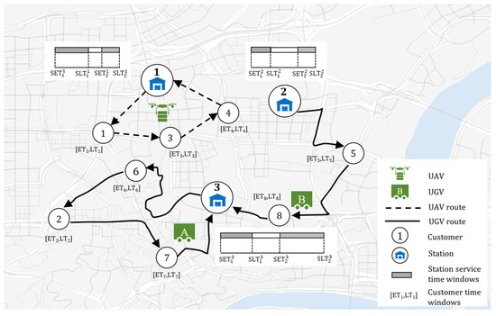
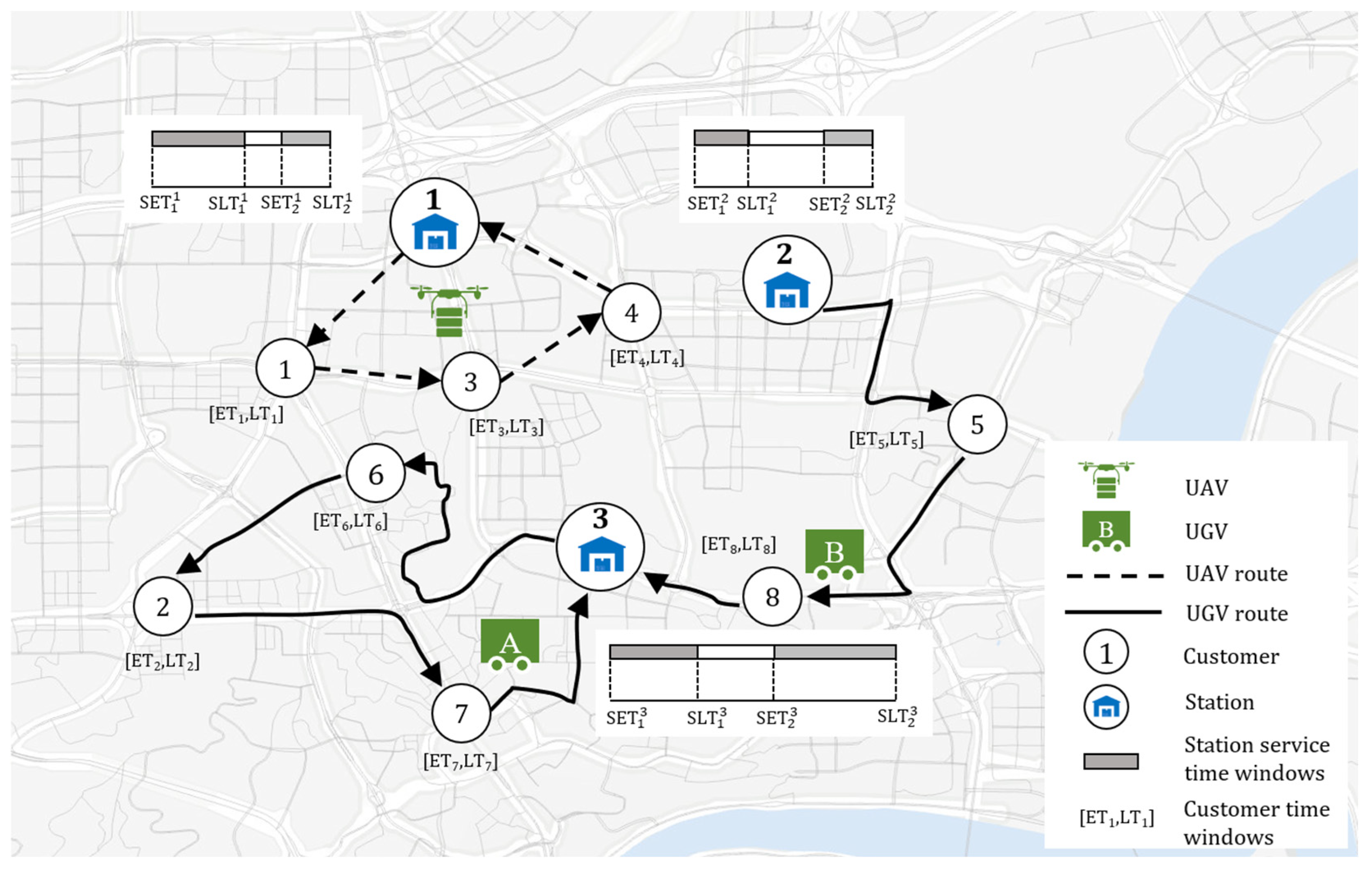
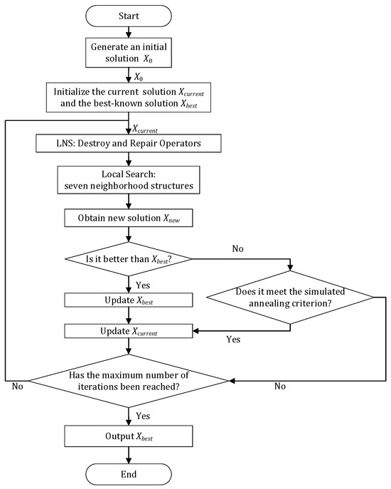
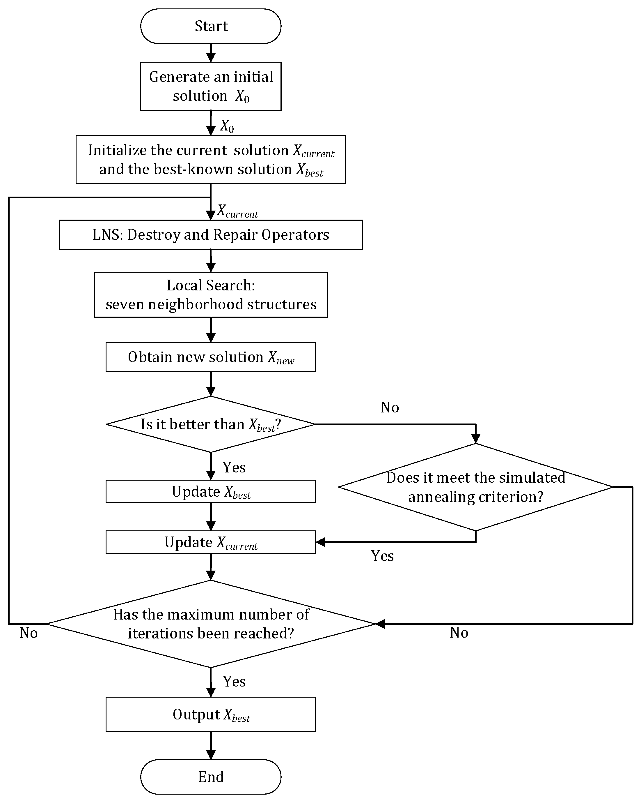
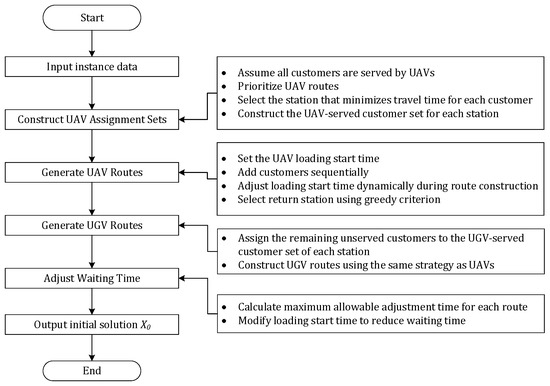
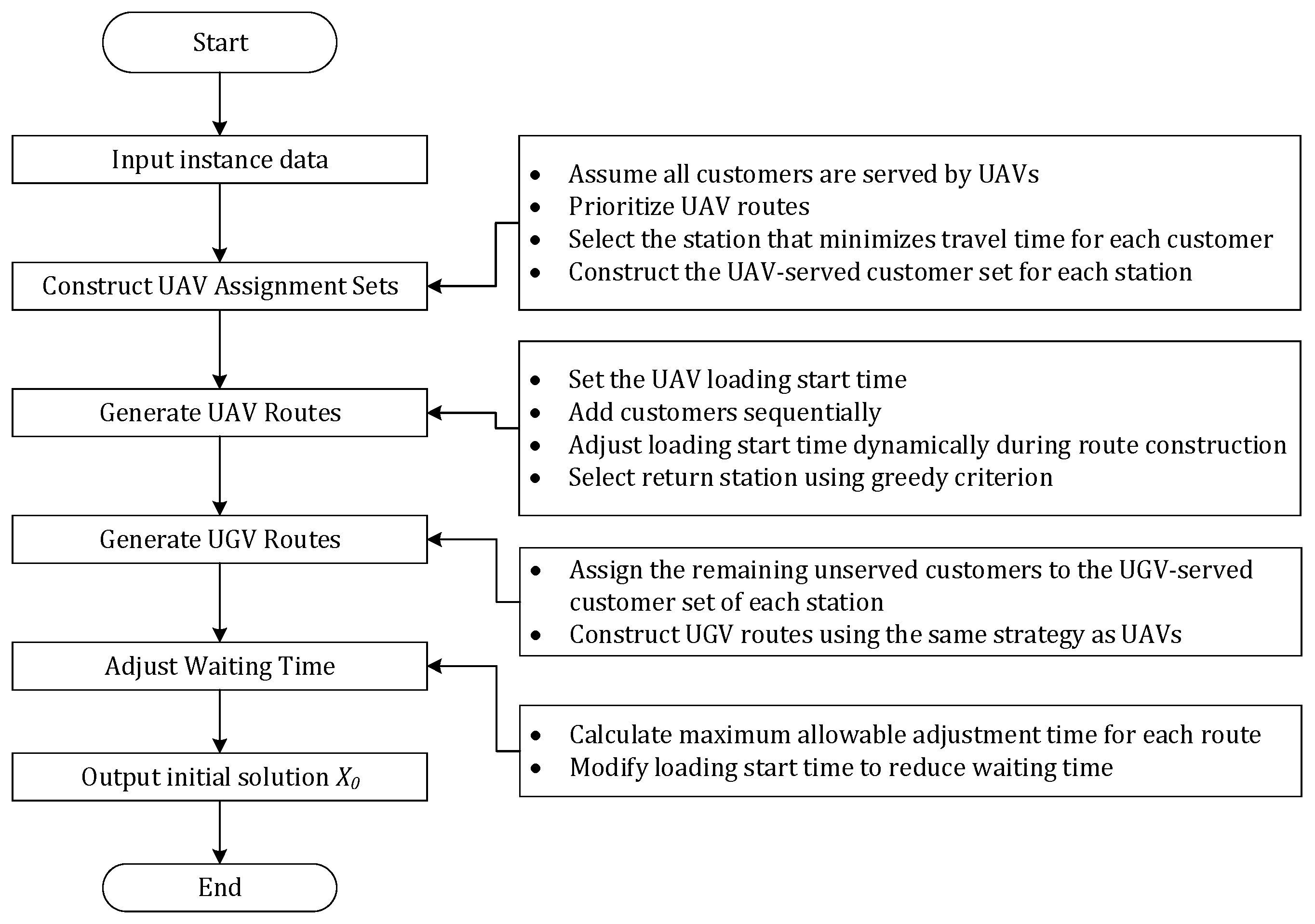
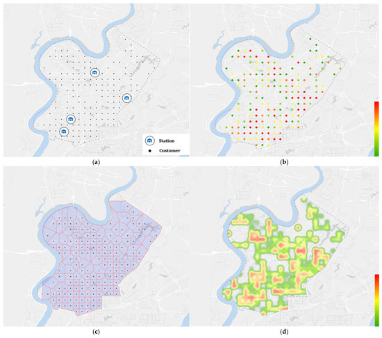
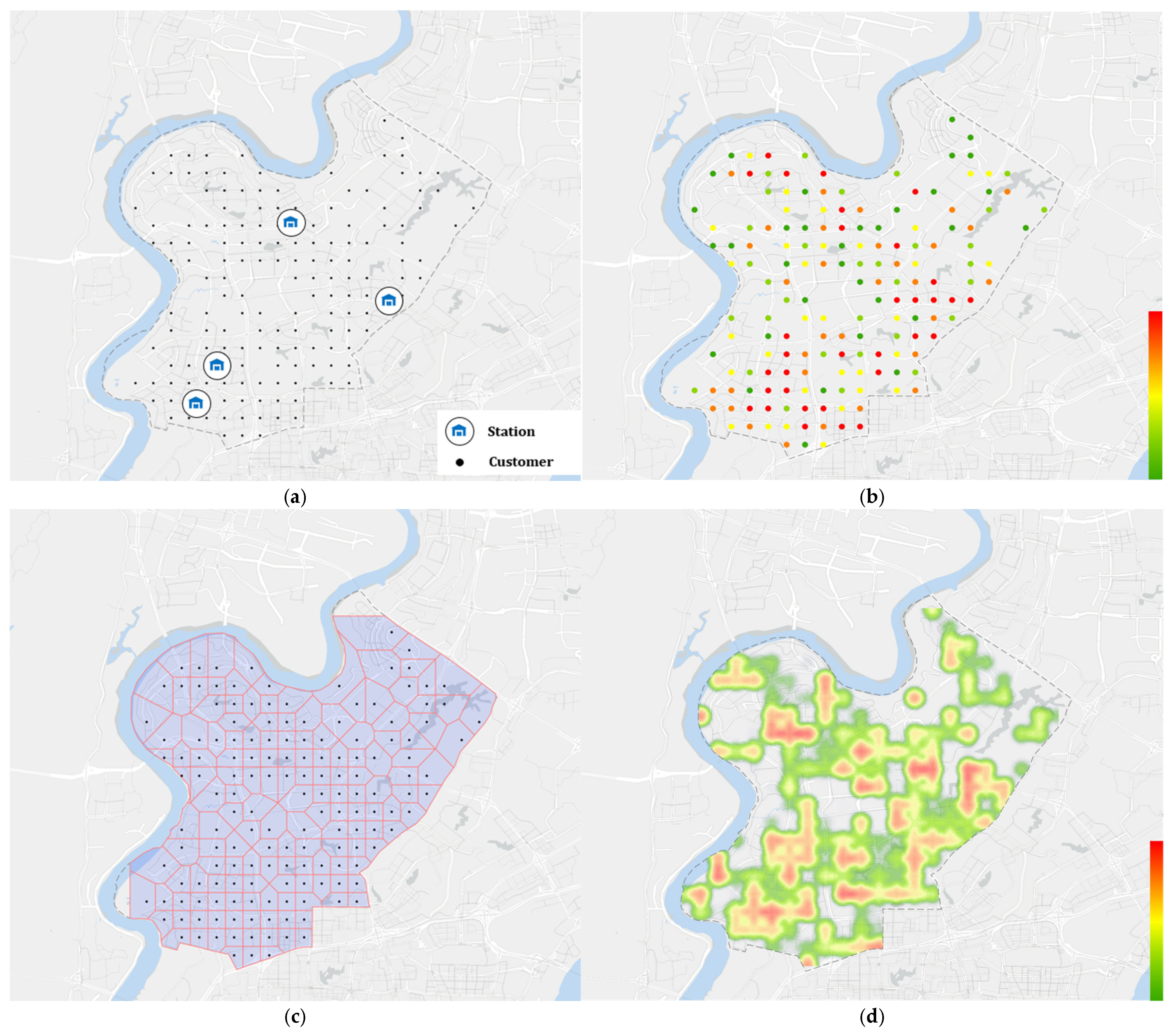
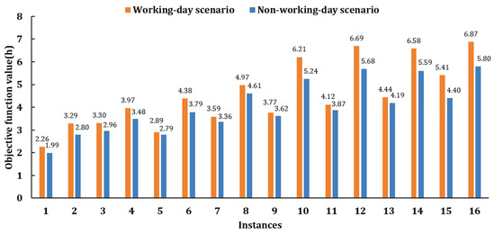
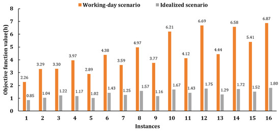
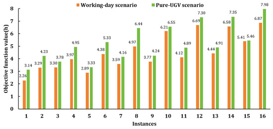
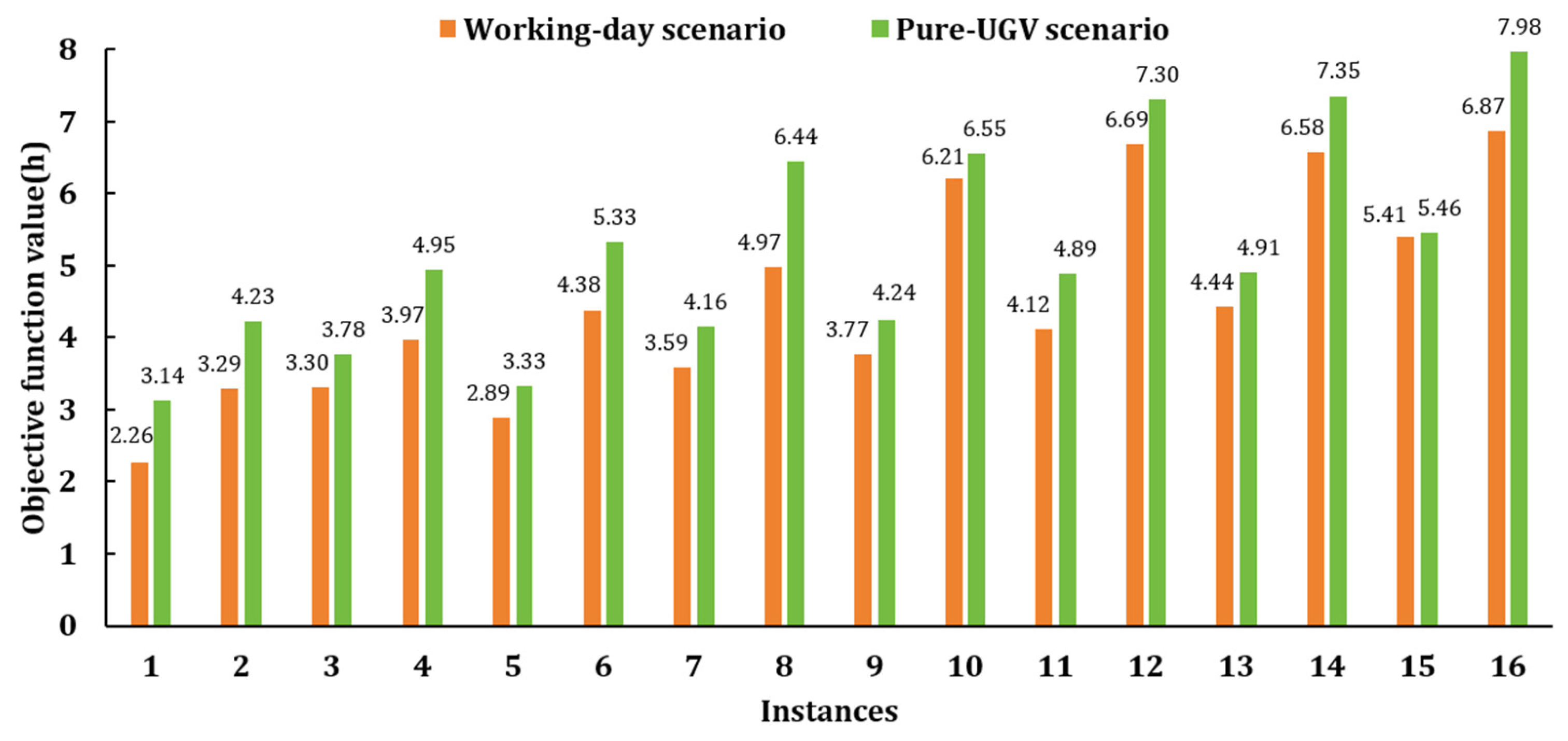
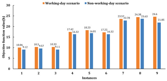
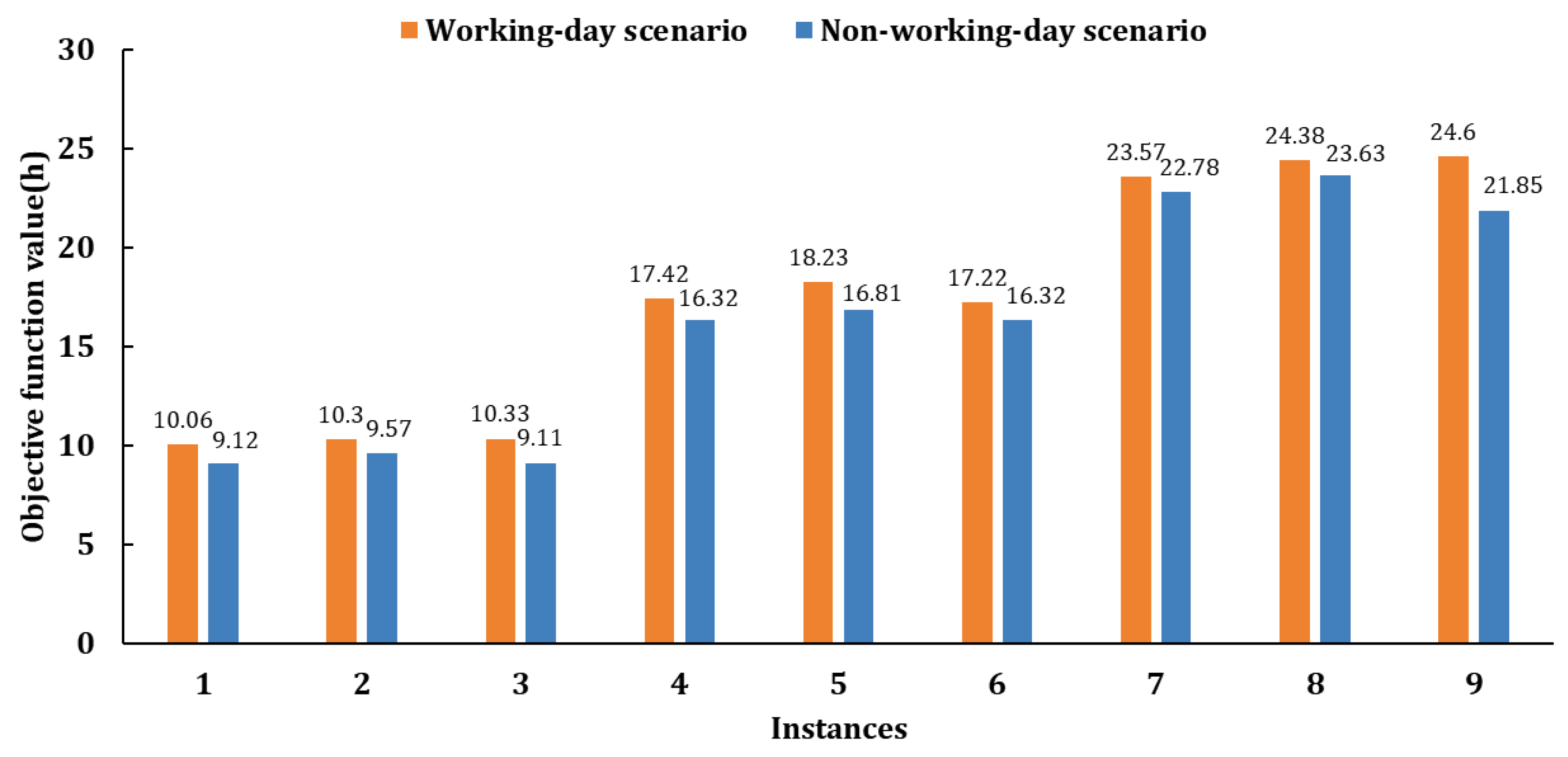
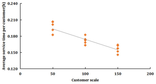
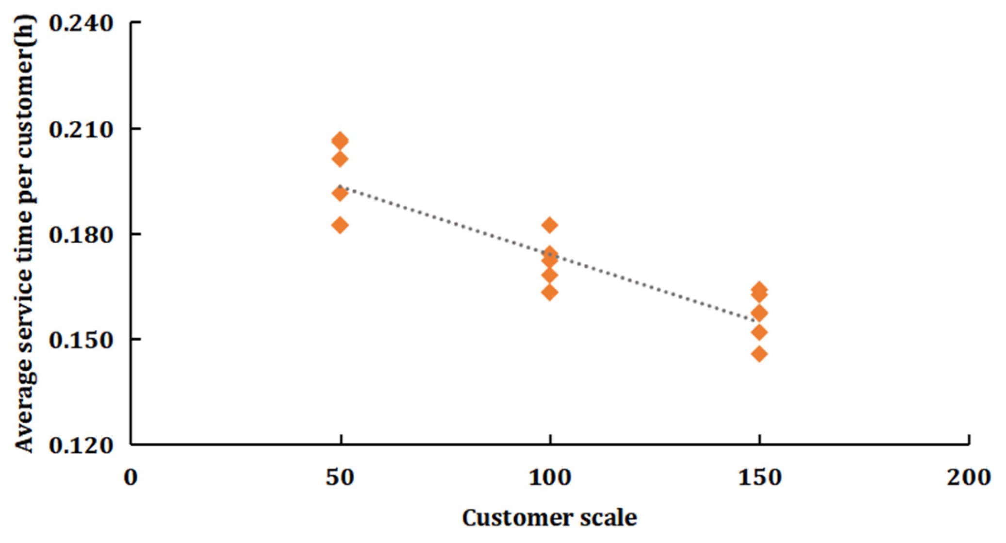
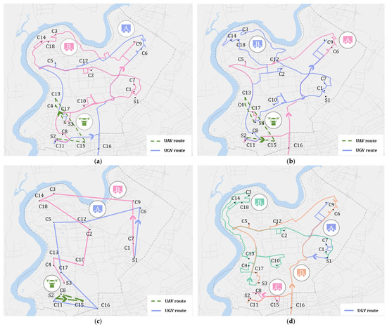
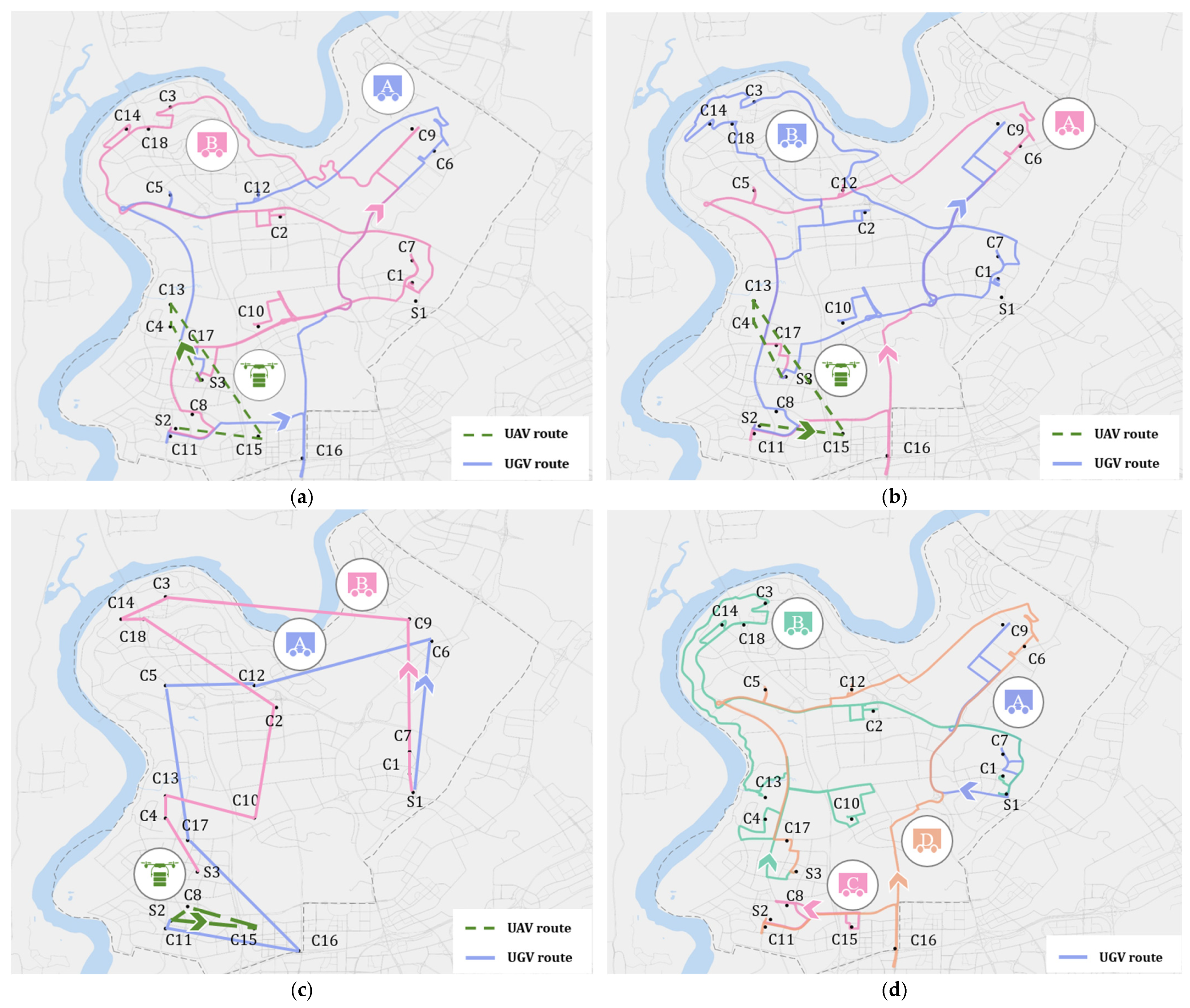
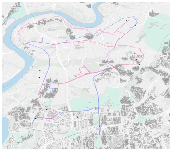
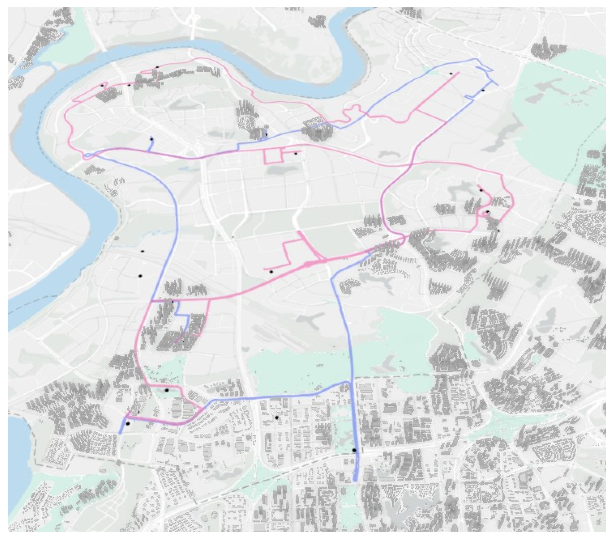

Disclaimer/Publisher’s Note: The statements, opinions and data contained in all publications are solely those of the individual author(s) and contributor(s) and not of MDPI and/or the editor(s). MDPI and/or the editor(s) disclaim responsibility for any injury to people or property resulting from any ideas, methods, instructions or products referred to in the content. |
© 2026 by the authors. Licensee MDPI, Basel, Switzerland. This article is an open access article distributed under the terms and conditions of the Creative Commons Attribution (CC BY) license.