


Highlights
What are the main findings?
- The median interval from centered offline alerts to listener responses reached 4.1 s across the paired observations.
- The BEATs detector achieved a held-out F1 0.901 across seven sessions containing 2282 one-second evaluation windows.
What are the implications of the main findings?
- Commodity smartphone microphones support low-cost warnings when airframe coverage and false-alert limits remain explicit.
- One-hour profiling met every processing deadline across four Android devices without observed thermal throttling.
Abstract
Smartphone microphones support low-cost acoustic monitoring, while co-located listener responses provide a timing reference for recorded drone approaches. This study evaluates Android acoustic detection using listener timing from five controlled flight sessions. Three listeners provide paired response times against a common audible-onset reference during those sessions. The sessions covered four DJI aircraft comprising Matrice 200, Matrice 300, Mavic 3, and Phantom 4. During every session, listeners and the phone shared one acoustic scene and common audible-onset reference. Centered alerts preceded listener responses by a median 4.1 s across fifteen paired observations. Session-clustered resampling placed the 95% interval for this paired difference between 2.2 and 6.7 s. Centered alerts occurred earlier in thirteen observations, while two Phantom 4 responses preceded those alerts. The seven held-out sessions contained 2282 one-second windows and yielded a BEATs F1 of 0.901. Centered score ranking achieved an ROC AUC of 0.991 and a PR AUC of 0.987 on held-out data. Sustained one-hour profiling met every processing deadline on four Android devices without observed thermal throttling. Dynamic INT8 quantization reduced model storage by 72.1% and inference latency by approximately 37%. Centered smoothing uses future scores, so these intervals describe offline timing within the recorded sessions.
1. Introduction
Small multirotor aircraft now create monitoring concerns around homes, infrastructure, and public events. Acoustic warning systems identify approaching aircraft from rotor emissions recorded within the surrounding sound environment. Radar, optical cameras, radio-frequency receivers, and acoustic sensors provide complementary evidence under different operating constraints. Personal warning systems rarely include dedicated radar units or calibrated microphone arrays because these sensors require specialized hardware. Most users carry smartphones with microphones and sufficient processing capacity for portable acoustic monitoring.
Optical and infrared cameras localize targets accurately when an unobstructed line of sight remains available. Darkness, occlusion, and background clutter can reduce their reliability across many low-altitude operating environments. Radio-frequency receivers detect control links but cannot observe autonomous aircraft or platforms operating without active transmitters. Radar extends detection range but requires costly hardware, substantial power, careful siting, and regulatory coordination. Acoustic sensing operates passively without illumination and responds to rotor emissions that accompany powered flight. It can operate independently or complement visual and radio-frequency evidence within a multisensor warning system [1,2]. Smartphones trade array gain and direction finding for wide availability, portability, and negligible added hardware cost.
The related Zenodo record accompanies a companion field study and describes its broader non-audio archive. Version DOI https://doi.org/10.5281/zenodo.19288594 belongs to the concept record identified by DOI https://doi.org/10.5281/zenodo.19288593. This manuscript analyzes the accompanying score-level supplement, retaining its recorded session assignments and decision settings. The repository description reports 33/7/7 session partitions, while this supplement records 36/4/7 partitions. Companion-study summary values therefore remain separate from the held-out results calculated for the present manuscript. The public metadata also describe open-field and lightly urban scenes with approach distances between 10 and 120 m.
Recent acoustic studies use learned representations, harmonic features, and multimodal fusion across varied operating conditions [3,4,5,6]. Public UAV corpora enable repeated evaluation, although airframe diversity and environmental coverage remain limited [7]. BEATs provides pretrained acoustic-token representations for environmental sound classification under varied recording and environmental conditions [8]. Other studies compare Transformer encoders, attention mechanisms, compact networks, and metric-learning objectives for acoustic recognition [9,10,11,12,13,14,15]. Smartphone studies also document microphone capability, resource limits, and sustained inference constraints during on-device acoustic processing [16,17,18,19,20,21].
Recent UAS perception studies distinguish noticeability from affective responses, while psychoacoustic models predict short-term noise annoyance [22,23]. These endpoints describe perceptual experience without supplying the paired first-response timestamps examined in this manuscript. Edge audio studies also cover daily routines on STM32L4 nodes and federated urban-sound recognition on ESP32 devices [24,25]. A recent survey reviews anomalous sound detection on edge systems and their implementation constraints [26]. Those application settings provide deployment context, although their reported workloads differ from the sustained Android drone inference evaluated here.
Several measurement problems motivate this evaluation of practical smartphone drone-warning performance under field conditions. Published systems usually compare algorithms across different corpora instead of directly measuring attentive human listeners. Window-level metrics can conceal fragmented alerts that users experience as repeated warning episodes [27,28,29]. Connecting these measurements requires listener timing and explicit accounting for continuous alert episodes. Device feasibility also requires sustained measurements of timing, memory, thermal behavior, and battery consumption.
The major contributions of this work concern the following three evaluation problems.
- (1)
- Lotinga and colleagues assess noticeability through source-selection judgments after playback, without timestamping paired smartphone alerts [22]. The present paired records quantify first-response timing relative to detector alerts within the same acoustic scene. Three co-located listeners contribute fifteen observations across five flights using a common audible-onset clock. This pairing removes recording-scene differences from the timing reference and retains the observed airframe-dependent responses.
- (2)
- Window-level detector comparisons leave individual false-alert durations unspecified by their aggregate false-positive rates. The decision analysis adds episode counts and durations using the same archived scores as the classification evaluation. Centered smoothing and causal replay expose different timing and nuisance behavior under explicitly defined decision rules. Separate held-out comparisons retain the original session assignments, while complete-archive sweeps examine threshold and run-length sensitivity.
- (3)
- Trigkas and colleagues report ESP32 inference and communication costs while leaving energy measurements unresolved [25]. The one-hour Android traces here document sustained drone inference together with memory, temperature, and battery observations. These measurements establish the recorded processing requirements across four handset classes within the same profiled workload. The accompanying FP32 and INT8 measurements quantify storage and latency reductions alongside the retained classification results.
2. Materials and Methods
2.1. Experimental Campaign and Physical Setup
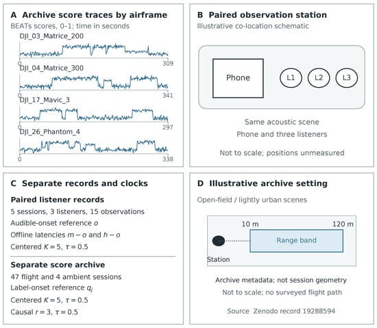
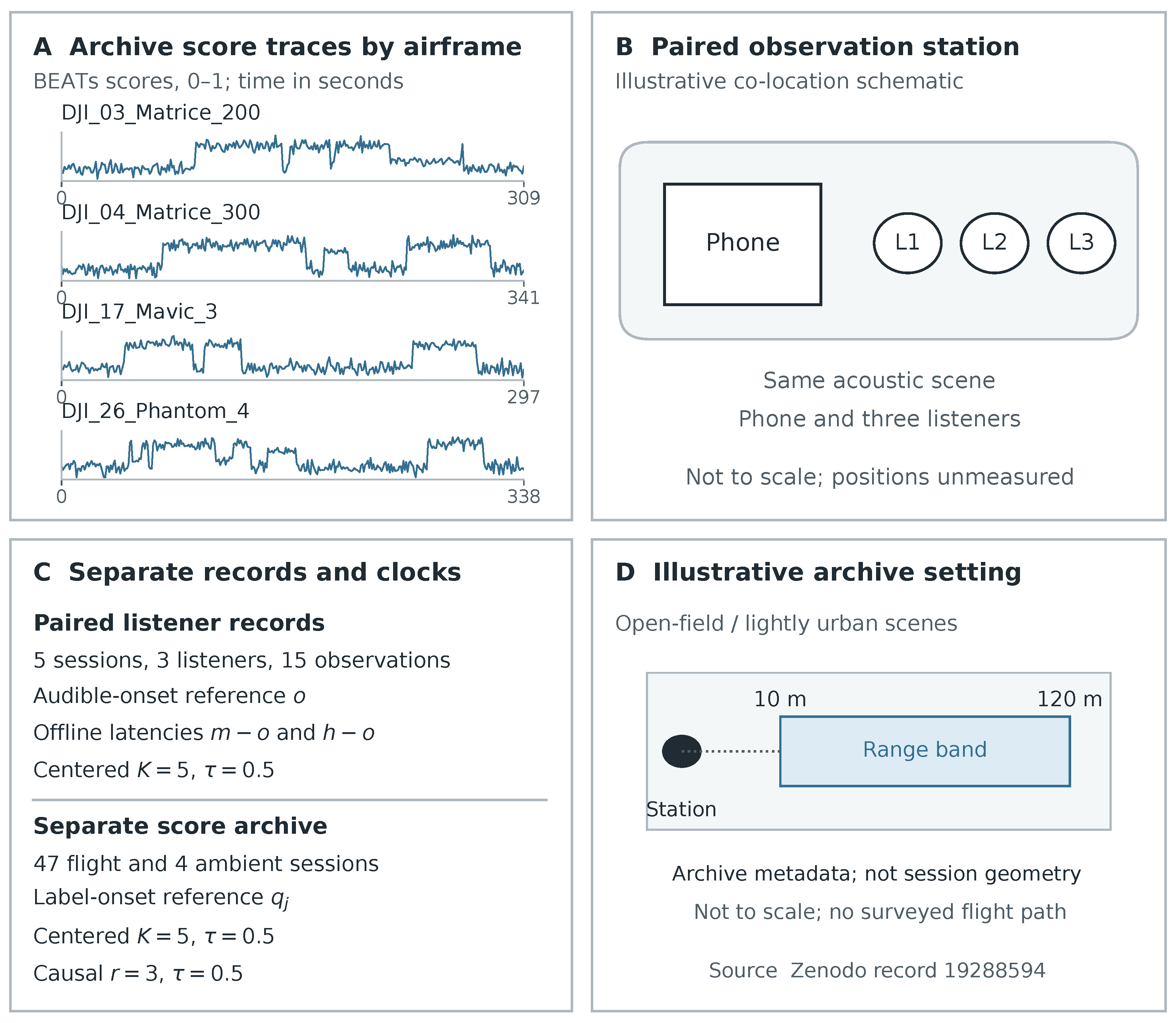
The study combines paired listener observations, a field score archive, and sustained Android device profiling. Figure 1 connects the documented airframes and recorded scores with the paired station and analysis clocks. Panel D illustrates the 10–120 m approach range reported in the public metadata for the companion archive. This range supplies recording context without assigning distances or coordinates to particular paired sessions. Per-session positions, flight altitudes, and the paired-station smartphone identity remain absent from the supplied score-level files. The flight sessions cover DJI Matrice 200, Matrice 300, Mavic 3, and Phantom 4 aircraft (SZ DJI Technology Co., Ltd., Shenzhen, China). The sustained profiling covered four phones. These include OnePlus Nord (OnePlus Technology (Shenzhen) Co., Ltd., Shenzhen, China) and Xiaomi Redmi 12 (Xiaomi Communications Co., Ltd., Beijing, China). The Galaxy S22+, Galaxy A52M, and OnePlus Nord records list Snapdragon 8 Gen 1, Snapdragon 750G, and Snapdragon 765G system-on-chips, respectively (Qualcomm Technologies, Inc., San Diego, CA, USA); the Redmi 12 record lists a Helio G88 system-on-chip (MediaTek Inc., Hsinchu City, Taiwan). The designation Galaxy A52M is retained as recorded in the profiling archive.
Figure 1.
Panel (A) shows archived traces for the four documented DJI airframes; the blue line in each thumbnail represents the BEATs detector confidence score. Each thumbnail uses the first held-out session for that airframe after sorting session identifiers. These traces show recorded detector scores, not log-mel spectra. Panel (B) places the phone and three listeners within an illustrative shared station plan. Panel (C) distinguishes the paired audible-onset clock from the label-onset clock in the score archive. Panel (D) illustrates the metadata range of 10–120 m in open-field and lightly urban recording contexts. Station positions and approach direction are schematic, without measured geographic coordinates or session-specific trajectories.
The profiling environment used Android 12 or later (Google LLC, Mountain View, CA, USA); Android 12 corresponds to API level 31. Individual operating-system build identifiers were not retained. The primary detector used the BEATs-iter3 encoder from the Microsoft UniLM/BEATs model family (Microsoft Corporation, Redmond, WA, USA). The model identifier BEATs-iter3 denotes the third training iteration in the official distribution (https://github.com/microsoft/unilm/tree/master/beats, accessed on 22 June 2026). The Compact CNN and MFCC+SVM baselines are custom detector pipelines represented by the score outputs. For the paired-listener experiment, the supplied score-level records do not retain the manufacturer or model of the smartphone used at the paired station or of the manual listener-response button. No chemical or biological agents or reagents were used.
2.2. Acoustic Features and Detection Models
The released archive stores one-second confidence scores for three acoustic detection pipelines used throughout the analysis. BEATs supplies primary scores through pretrained acoustic-token representations for environmental sound classification [8]. The Compact CNN derives scores from log-mel spectrogram inputs evaluated at the same one-second window granularity. The classical baseline classifies mel-frequency cepstral coefficients with a support vector machine at each window.
The supplied package supports score-level evaluation from stored detector outputs and retained session metadata. Its files omit raw audio, model checkpoints, optimizer settings, SVM hyperparameters, and feature extraction configurations. The repository description separately lists derived log-mel features, model checkpoints, and training code within its restricted archive. It specifies three-second analysis windows advanced by one-second hops for the companion study. The present score-level analyses use the retained one-second cadence without reconstructing unavailable audio inputs or spectral features.
2.3. Field Score Archive
The archive contains 47 flight sessions and four ambient negative sessions recorded for detector evaluation. Together, these sources contain 24,881 one-second score rows supporting all reported decision analyses. The flight subset includes 19,481 one-second rows from four DJI airframes summarized in Table 1. Each archive row stores its session identifier, time index, binary presence label, and three detector scores. All three detectors share the same rows, time indices, and binary reference labels throughout evaluation. Metadata assign 36 sessions to training, four to validation, and seven to held-out testing. Each flight session appears in exactly one predefined data partition to prevent cross-partition reuse. All four airframes occur within the seven-session held-out test partition used for final evaluation. Section 3.2 reports held-out values alongside the complete performance summary used across all three partitions.
Table 1.
Flight score archive composition by DJI airframe and predefined training, validation, and test partitions. The held-out test partition contains seven sessions and 2282 windows covering all four evaluated airframes.
The ambient panel contains four 1350 s sessions without positive drone presence labels in any row. Recorded conditions include urban traffic, nearby speech, open-field wind, and mixed park noise. Together, these ambient sessions provide a bounded nuisance check covering 1.5 recorded hours in total. Nuisance evaluation counts alerts during this negative exposure after applying each specified decision rule. Section 2.7 defines the Poisson upper limit used when the observed event count equals zero. The short exposure restricts interpretation to the recorded conditions represented within this ambient panel.
2.4. Paired-Listener Test Panel
The released human baseline file contains fifteen observations from three listeners across five paired flight sessions. Matrice 200 appears in two sessions, while each remaining airframe appears in one session. Listeners and the smartphone shared the same acoustic scene at one station during every paired flight session. Each listener pressed a button upon first hearing the approaching aircraft during every session. The available record does not retain participant ages, audiometric screening, prior familiarity, or training history. Those missing characteristics prevent stratified listener analyses across the available paired observations.
Each paired row stores the audible onset o, model alert m, and listener response h timestamps. Model latency equals , whereas listener latency equals for the same observation. The difference defines a positive offline model advantage whenever model alert precedes listener response. The smartphone scores use centered smoothing with and the fixed threshold . Centered smoothing uses two future one-second rows and remains noncausal during replay. These paired latencies characterize offline timing without supporting a streaming comparison.
One annotator assigned the common audible-onset reference after reviewing audio from each recorded session. A second annotation pass occurred two weeks later and differed by at most one second. The supplied five-session listener package contains no independent audible-onset assessment from another annotator for comparison. This single-annotator onset reference limits confidence in the reported latency differences.
2.5. Device Profiling Protocol
The profiling files document one-hour sustained detector inference across four Android devices. These devices define the operating-system scope of the measured deployment results reported below. The set included one flagship device, two mid-range devices, and one budget device. Each device contributed 3600 latency rows and an equal number of sampled memory observations. CPU, thermal, and battery traces used lower sampling frequencies than the corresponding latency measurements. A separate profiling file compares FP32 measurements with results from a dynamically quantized INT8 export.
2.6. Alert Decision Framework
Let session j contain ordered one-second rows indexed from 1 through for analysis. Score belongs to binary label for each row in that session. Alert state takes a binary value for every corresponding row within the same session. The indicator function equals one when its stated condition holds. Superscripts and distinguish centered and causal alert states; denotes the state under the rule being evaluated. Let denote the first positive archive row observed within flight session j. The indicator below records whether any positive row also carries an alert.
The following expression measures first-alert latency from the first positive archive row within each detected session.
Because adjacent archive rows are one second apart, is expressed in seconds. A false-alert event is any maximal alert run occurring during consecutive negative rows. Its event count, longest run, and singleton count summarize the false-alert distribution.
Both reported decision rules apply the common score threshold value throughout replay. The offline rule averages an odd number K of centered score rows around each time index.
For each index, contains available rows from through inclusively within that session. The set becomes shorter only near the beginning and end of each session. The analysis uses , which incorporates up to two future score rows for each index. The causal rule processes scores in forward order and requires r consecutive threshold crossings.
A run length of three defines the default setting for causal score replay. The sensitivity analysis also reports run lengths from one through five consecutive threshold crossings. Missing score streams prevent direct causal recomputation for the five paired listener sessions.
The validation split alone selects every tuned score threshold subsequently applied during held-out testing. All test rows receive that fixed threshold without additional tuning or score recalibration.
2.7. Evaluation Metrics
Window-level evaluation compares each binary alert decision with the presence label on the corresponding archive row. True positives (), false positives (), true negatives (), and false negatives () accumulate within the stated evaluation partition. The following equations define precision, recall, F1, and false-positive rate from those accumulated confusion counts.
Partition-level values pool the relevant rows while retaining their predefined session assignments throughout evaluation. Held-out model comparisons use identical test rows and labels for every detector in the comparison. Complete-archive summaries also include training and validation sessions, as indicated beside those reported values.
Event-based scoring groups consecutive alert rows into predicted events within each individual recording session. Consecutive positive reference labels define the reference events used for the corresponding onset comparison. Greedy nearest-onset matching assigns each predicted run to the closest unmatched reference onset within a one-second collar. Each matched pair contributes one true positive, and unmatched predictions and references contribute false positives and false negatives. Event precision, recall, and F1 apply the same count definitions after replacing rows with matched events. This onset criterion follows the sound event detection practice underlying the reported event analysis [27,28].
ROC AUC measures score ranking across thresholds within the partition identified beside each result. The reported PR AUC uses average precision, summing precision over increases in recall along the ranking. Centered scores underlie the held-out ranking values, while the complete-archive ranking curves use raw detector scores. Ranking measures do not depend on the subsequently chosen binary decision threshold for that score sequence.
Paired timing measures use the common audible onset, model alert, and listener response timestamps within each observation. Model and listener latencies subtract that audible onset from their respective recorded timestamps. The paired margin subtracts the model alert time from the corresponding listener response time. Positive margins indicate earlier centered alerts, and negative margins indicate earlier responses from the paired listener. Archive first-alert latency instead uses the first positive label through the definition in Section 2.6. These separate onset references remain attached to their respective results throughout the analysis.
False-alert accounting counts maximal alert runs occurring entirely within consecutive drone-absent score rows. Event frequency divides that count by the corresponding drone-absent exposure expressed in hours. Longest-run duration and singleton counts describe the persistence and fragmentation of those nuisance episodes. For zero observed events, a Poisson model gives the following one-sided 95% upper rate limit.
The four ambient recordings supply this exposure, giving the reported rounded limit of 2.0 events per hour. Applying this limit beyond the observed ambient conditions would require additional representative negative recordings.
Bootstrap intervals resample complete sessions with replacement, preserving temporal dependence among rows within each selected session. Paired-listener resampling keeps all three observations together whenever a replicate selects their shared flight session. Each reported interval identifies its session population and bootstrap replicate count in the results. The small paired panel supports descriptive uncertainty estimates across its five recorded sessions.
2.8. Listener Subset Sensitivity
The sensitivity analysis enumerates every subset containing one, two, or three recorded listeners within each paired session. The earliest response in each subset defines its panel response time for this descriptive calculation. For session j and its listener set , the following averages define subset latency and margin.
The timestamps and denote the shared audible onset and centered model alert within session j. Averaging these session summaries equally across the five flights gives the reported descriptive means. Each flight supplies three individual subsets, three two-listener subsets, and one complete three-listener subset. Overlapping subsets reuse observations, so uncertainty calculations cannot treat them as independent experimental samples.
3. Experimental Results and Analysis
3.1. Smartphone and Human Listener Latency
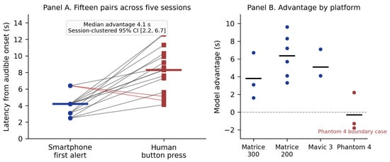
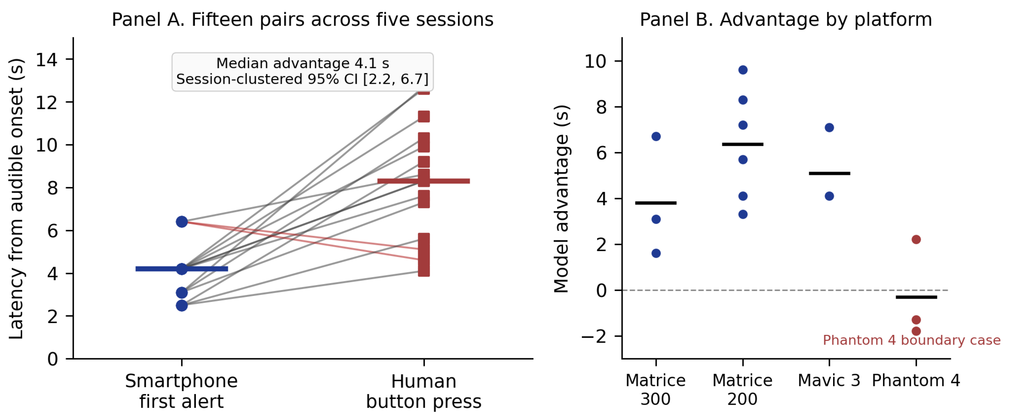
The offline paired timing analysis contains fifteen listener-session observations from five controlled flight sessions. Centered alerts preceded listener responses by 4.27 s on average, with a median difference of 4.1 s. Table 2 summarizes the listener latencies, and Figure 2 shows all fifteen paired observations and the median margin. A 10,000-replicate session-clustered bootstrap across five clusters produced the descriptive interval seconds. Centered alerts preceded responses in thirteen observations, while two Phantom 4 responses occurred before the corresponding alerts.
Table 2.
Offline comparison between smartphone and human listener latency from audible onset across five sessions. Values represent means plus or minus standard deviations for each listener and the pooled observations.
Figure 2.
Offline smartphone and listener latencies from each session’s common audible onset. In Panel (A), blue circles denote centered smartphone alerts, red squares denote listener button presses, and matching colored bars show medians. Gray connecting lines identify earlier smartphone alerts; the two red connecting lines identify earlier listener responses. Coincident observations overlap. In Panel (B), blue dots represent Matrice 200, Matrice 300, and Mavic 3 observations; red dots represent Phantom 4. Black bars show airframe-specific mean advantages, and the gray dashed line marks zero. Centered smoothing uses up to two future seconds and is noncausal.
Matrice 200 produced a mean difference of 6.37 s across six paired comparisons. Mavic 3 produced 5.10 s, and Matrice 300 produced 3.80 s across three comparisons each. Phantom 4 produced a mean difference of s across its three comparisons. Two Phantom 4 listeners responded earlier than the centered smartphone under these limited session counts. These airframe findings therefore remain descriptive across the five controlled flight sessions.
Sensitivity to Listener Subset Size
Table 3 reports first-response timing from all available listener subsets within each of the five recorded sessions. Mean first-response latency decreases from 8.37 s for individual listeners to 6.38 s for three listeners. Corresponding mean response-minus-alert margins decrease from 4.29 s to 2.30 s across those observed subsets. The two-listener calculation gives a 6.87 s mean response latency and a 2.79 s mean margin. This decrease follows from choosing the earliest response among progressively larger subsets of the same recorded listeners. The centered model alert remains an offline reference throughout this descriptive reanalysis.
Table 3.
Listener-subset sensitivity using the earliest recorded response within each subset across five paired flight sessions. Latencies share the audible-onset reference, while margins subtract the centered model alert from that earliest response. These descriptive means reuse dependent observations and therefore carry no subset-level confidence intervals.
The subset calculation used timestamp differences, whereas the original pooled summary used the archived derived-margin column. Three stored margins differ from their corresponding timestamp differences by 0.1 s within the supplied source file. The original reported mean remains 4.27 s, while direct timestamp subtraction gives 4.29 s for individual listeners. The supplementary consistency table identifies these rows and preserves all original source values.
3.2. Held-Out Detection Performance
Table 4 reports centered BEATs performance at threshold for training, validation, and held-out test partitions. The held-out partition contained 2282 windows from seven sessions covering all four airframes without session overlap. BEATs reached a held-out precision of 0.952, recall of 0.854, window-level F1 of 0.901, and false-positive rate of 0.031. The held-out ROC AUC reached 0.991, while the PR AUC reached 0.987 across those seven sessions.
Table 4.
Centered BEATs using and across three partitions, including strict held-out evaluation over seven test sessions.
F1 decreased from 0.973 during validation to 0.901 on held-out sessions. Two held-out sessions produced false-positive rates near 0.09 under the same decision rule. The other five test sessions produced F1 values between 0.834 and 1.000 under centered smoothing.
For the detector comparison, Table 5 uses identical held-out rows, labels, and session assignments across all three models. BEATs exceeded Compact CNN’s window-level F1 by 0.052 across the seven held-out sessions. The archive bootstrap in Section 3.5 uses every flight partition, providing a separate descriptive comparison.
Table 5.
The centered-rule comparison evaluated three models on the held-out test partition containing seven sessions and 2282 one-second windows.
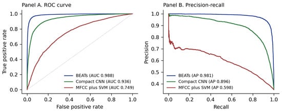
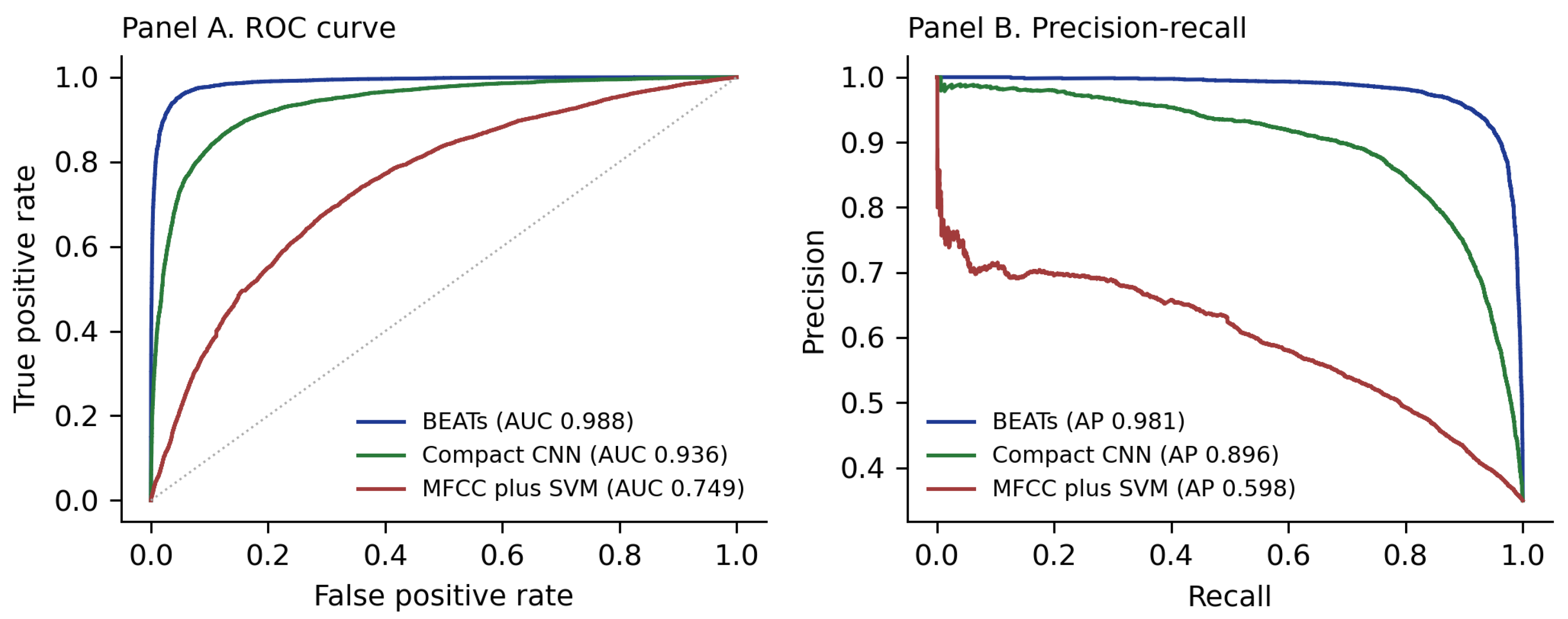
Figure 3 shows the separate raw-score ROC and precision–recall curves over the complete flight archive. Published studies use different recordings, sensors, partitions, scoring intervals, and event criteria, preventing direct numerical comparison. The quantitative analysis compared only models sharing identical rows, labels, and test sessions.
Figure 3.
Raw-score ranking over 19,481 flight rows from all archive partitions. Panel (A) shows receiver operating characteristic curves, and Panel (B) shows precision–recall curves. Blue, green, and red curves represent BEATs, Compact CNN, and MFCC plus SVM, respectively. The gray dotted diagonal in Panel (A) is the chance-ranking reference, where the true-positive rate equals the false-positive rate and ROC AUC is 0.5. PR legend values are average precision. These complete-archive curves are distinct from the held-out metrics in Table 5.
3.3. Validation-Tuned Threshold
The analysis fixed the default threshold before examining any test sessions. For a second operating point, a validation-only sweep across selected at a maximum F1 of 0.983. This fixed validation threshold produced a test F1 of 0.937, precision of 0.924, recall of 0.950, and false-positive rate of 0.057. This operating point favored recall, while the default threshold retained fewer false positives in Table 6.
Table 6.
Comparison of default and validation-tuned thresholds on the seven-session held-out test split without additional test tuning.
3.4. Event-Based F1 with Onset Collar
Table 7 reports descriptive event-based F1 across all 47 flight sessions, including every supplied data partition. Each predicted run matches one reference run within the predefined one-second onset collar. Across 118 references, BEATs reached an archive event F1 of 0.627, while Compact CNN reached 0.166. MFCC plus SVM reached 0.076 within the same archive event comparison. These archive values cover every partition and do not estimate held-out event performance.
Table 7.
Event-based evaluation applying a one-second onset collar to 118 annotated reference events across all 47 archive sessions.
Event-based and window-level rankings identify BEATs as the strongest archive detector, despite different absolute metric values. Event scoring penalizes fragmented and shifted runs under established sound event detection recommendations [27,28].
3.5. Session-Clustered Bootstrap of the Model Difference
A descriptive bootstrap compared BEATs and Compact CNN across all 47 flight sessions using 2000 resamples. Complete sessions formed each replicate, producing a mean archive window-level F1 difference of 0.092. The interval covers training, validation, and test partitions and remains a descriptive archive result. Table 5 provides the separate detector comparison across seven held-out sessions using identical test rows.
3.6. Causal Stream Replay and False-Alert Events
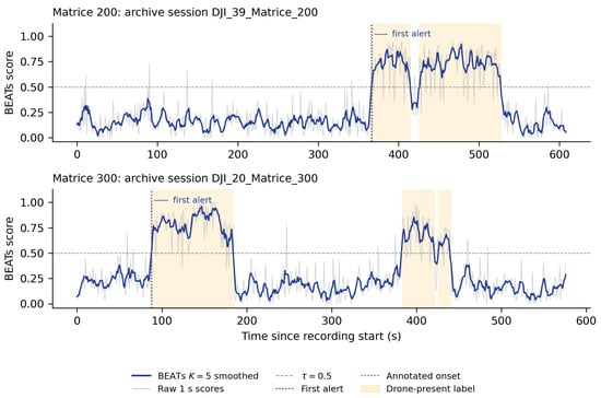
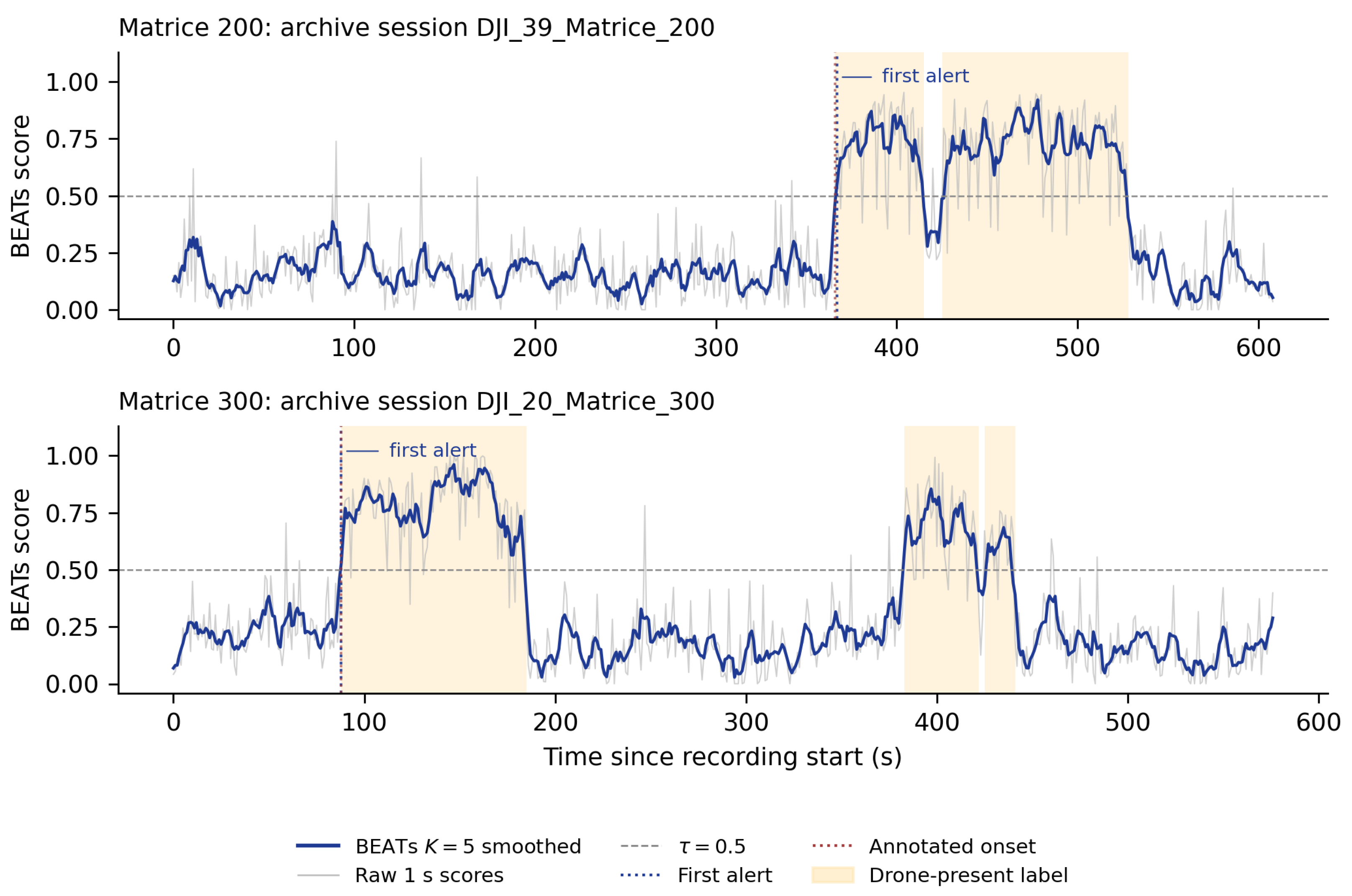
The archive supports a separate forward-ordered causal replay requiring three consecutive threshold crossings. The replay detected all 47 flight sessions with median label-relative delay of 2 s and IQR of seconds. The centered archive rule produced a median delay of 1 s with an IQR of seconds. Figure 4 shows representative scores and decisions from two archive sessions using their label-onset references. Those archive delays used label onset, whereas the listener panel used its separate audible-onset clock. The differing onset references prevented transferring these archive delays to the listener observations.
Figure 4.
Representative BEATs scores and centered alert decisions for two archive sessions. Light gray lines show raw one-second scores, and blue lines show centered scores. Orange bands mark drone-present reference labels. Red dotted vertical lines identify the first annotated label onset, blue dotted vertical lines mark the first centered alert during drone-present rows, and gray dashed horizontal lines mark the threshold . The onset and first-alert markers may coincide at the one-second archive resolution.
Raw thresholding produced 186 false-alert events within negative flight rows, including 180 isolated single-second events. Applying centered smoothing reduced this count to 14 events, and causal run filtering reduced it to seven. Table 8 reports these counts alongside a longest causal false-alert episode lasting 19 s. Event counts complement row-level false-positive rates when assessing deployment behavior from archived score sequences.
Table 8.
Table grouping false-alert events during drone-absent time by source and decision rule across evaluated recordings.
Raw thresholding produced 65 singleton ambient events across the four supplied acoustic conditions. Centered and causal rules removed every event from these 5400 s of score rows. These zero-event observations gave a 95% Poisson upper limit of 2.0 events per hour. This limit covers only supplied conditions, where Compact CNN produced two centered events and SVM produced 29.
3.7. Threshold and Run-Length Sweeps
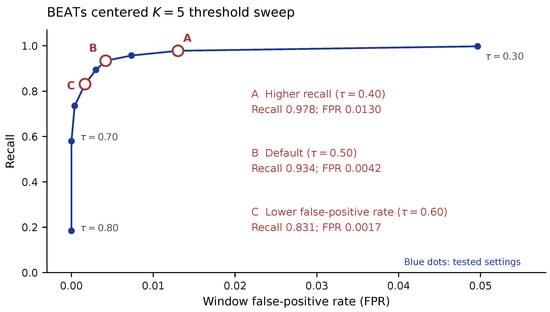
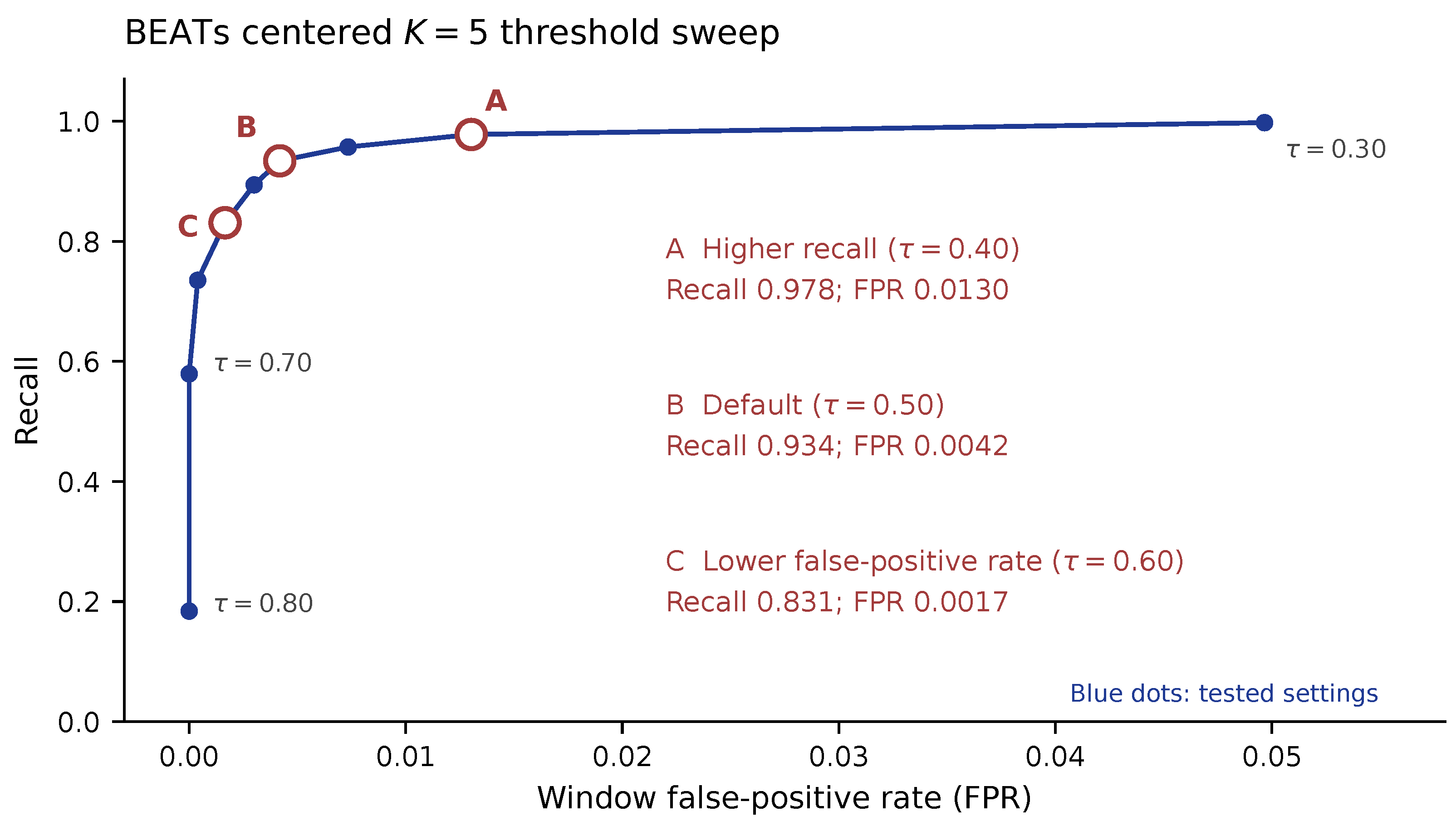
Table 9 reports selected settings from the centered threshold sweep across every flight partition, and Figure 5 displays the full nine-point sweep and its three highlighted operating points. Thresholds 0.4 and 0.6 produced a recall of 0.978 and 0.831, with false-positive rates of 0.013 and 0.0017. The default threshold of 0.5 lies between those reported operating points for recall and false alerts.
Table 9.
BEATs’ centered threshold sweep covering the complete 47-session flight archive across all supplied data partitions.
Figure 5.
BEATs centered threshold sweep across all 47 flight sessions. Blue dots show recall and false-positive rate at nine tested thresholds spanning 0.30–0.80. Blue segments connect successive settings for visual guidance rather than interpolation. Open red markers show three policy settings: (A) , higher recall; (B) , default; and (C) , lower false-positive rate. Annotations give each point’s recall and false-positive rate.
Table 10 compares recall and false-alert suppression across causal run lengths from one through five. One crossing produced 230 false-positive rows and 186 events across all archived flight sessions. Two crossings reduced false-positive rows to 49 across the same archived flight sessions. Three crossings produced 44 false-positive rows and a median delay of 2 s. All five reported run lengths detected every flight session within this archive.
Table 10.
BEATs’ causal run-length sweep using over the complete 47-session flight archive and every supplied partition.
Different onset references and missing paired score streams prevented causal recomputation for those five listener sessions.
3.8. On-Device Profiling on Commodity Android Hardware
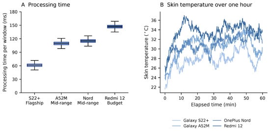
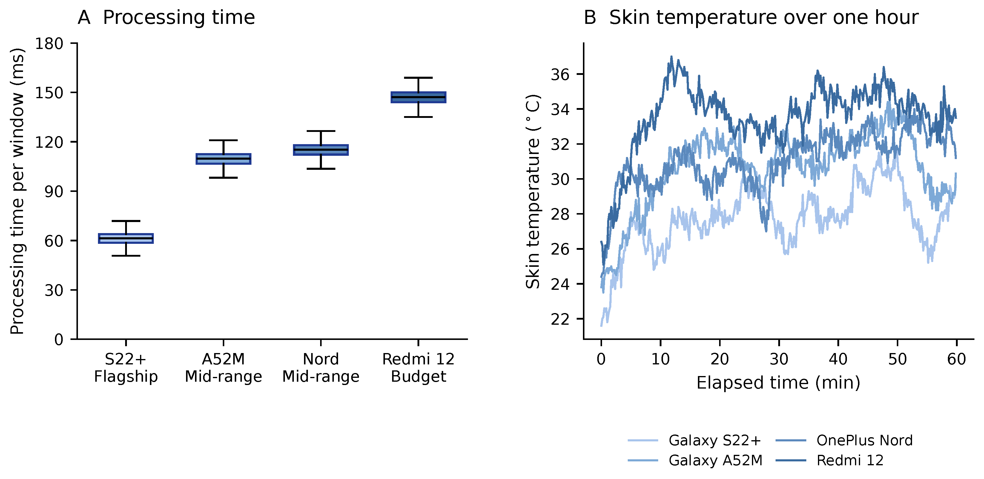
Table 11 reports one-hour profiling, and Figure 6 shows the processing-time distributions and skin-temperature traces. Every device met the one-second processing budget. Median processing times ranged from 61.3 to 147.2 milliseconds across these devices. Each device’s 99th percentile remained below 158 milliseconds during the same one-hour experiment. Mean steady memory ranged from 415 to 422 MB across the four devices. Their peak memory measurements ranged from 459 to 463 MB during profiling. Maximum recorded skin temperature reached 37 degrees Celsius on the budget phone. No thermal-throttle flag appeared during the complete one-hour traces from any evaluated device. Summary battery drain ranged from 2.8 to 5.6 percent per hour across the four devices.
Table 11.
Sustained one-hour device profiling evaluating deployed FP32 BEATs inference across four commodity Android phones.
Figure 6.
One-hour sustained profiling on four Android phones. Panel (A) shows processing-time distributions from 3600 windows per device. Boxes span the interquartile range, black lines mark medians, and whiskers extend to the most extreme observations within 1.5 interquartile ranges of the box; outliers are not drawn. The 1000 ms hop budget lies above the displayed 0–180 ms range. Panel (B) shows the original skin-temperature series. The legend identifies the same four blue device shades in both panels.
Mean total CPU use ranged from 13.7 to 26.4 percent across the four profiled devices. Mean inference-thread use ranged from 18.8 to 40.9 percent, excluding additional capture, logging, and interface workloads. Multi-day thermal and operating-system behavior remains unmeasured within the available one-hour device records.
3.9. Quantization Results
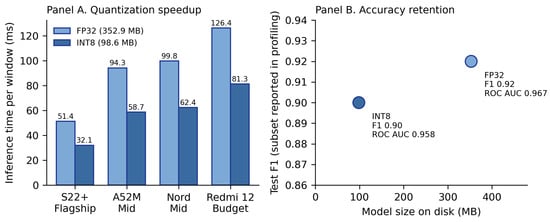
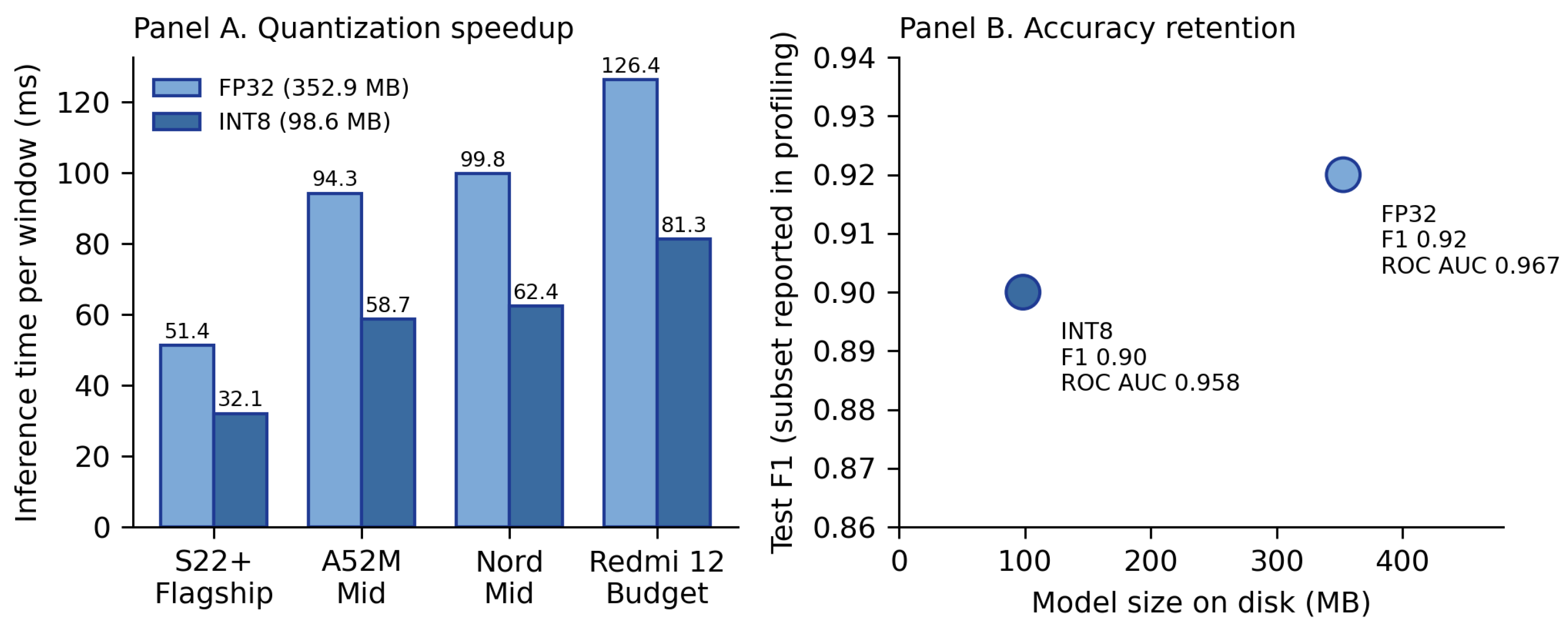
Figure 7 summarizes the inference-time and model-size comparison. Dynamic INT8 quantization reduced checkpoint storage from 352.9 to 98.6 MB. This storage change corresponds to a 72.1 percent reduction and 3.58-fold ratio. Reported peak inference memory decreased from 420 to 195 MB across the available profiling records. Median inference latency decreased by 35.7 to 37.8 percent across the four devices. The profiling subset retained an F1 of 0.90 and an ROC AUC of 0.958 after quantization, down from 0.92 and 0.967. The archive lacks quantized paired score streams for the five listener sessions. This absence prevented a corresponding analysis of listener timing after quantization.
Figure 7.
Dynamic INT8 quantization on four Android smartphones. In Panel (A), light blue bars show FP32 inference times, and dark blue bars show INT8 inference times for the same devices. In Panel (B), the light blue FP32 point and dark blue INT8 point show F1 against on-disk model size; nearby annotations give F1 and ROC AUC for the profiling subset. These profiling-subset metrics are separate from the seven-session held-out comparison.
4. Discussion
The five paired sessions yielded a 4.1 s median response-minus-alert interval, with the descriptive interval seconds. Two future rows contribute to that timing, so the comparison remains offline and does not represent a deployed alert. Phantom 4 remains a difficult case because two listeners responded first during its single recorded session. Only five sessions support that interval, which leaves airframe-specific inference unreliable across the recorded panel.
The held-out comparison assigned identical rows and labels to all three detectors across seven test sessions. BEATs produced a window-level F1 of 0.901, compared with 0.848 for Compact CNN and 0.601 for MFCC plus SVM. Published datasets use incompatible sensors and scoring designs, which prevented a valid external numerical ranking.
Causal replay within the separate 47-session archive required three consecutive crossings and produced seven false-alert events. The median label-relative delay was 2 s, but one false-alert episode continued for 19 s. A nineteen-second false alert remains operationally important for any future deployment trial.
All four Android devices met the processing budget throughout one-hour profiling, including the slowest phone at a median of 147.2 milliseconds. No thermal-throttle flag appeared, although behavior beyond one hour remains unknown in these records. INT8 quantization reduced storage by 72.1 percent and median inference latency by approximately 37 percent.
The listener panel included three people, five sessions, and one audible-onset annotator, without recorded ages or hearing assessments. The available files also omit familiarity and training histories, exact flight geometry, and the paired-station smartphone identity. These gaps restrict demographic, distance, altitude, and device-specific interpretation across the available observations. The subset analysis changed the response aggregation rule while retaining these same participants and acoustic scenes. Earliest-response margins decreased with subset size, and overlapping subsets remained dependent observations within each flight. This sensitivity describes the recorded panel without estimating a population response distribution for larger groups.
The supplied package supports score-level decision analysis and figure recomputation from shared rows and labels. It omits raw audio, model checkpoints, and complete training configurations needed for independent retraining. The public record describes a broader companion-study archive, including spectral features and detector checkpoints under restricted access. Its reported partitions and operating point differ from the settings retained in this score-level supplement.
Recent nonlinear dynamics studies examine synchronization and stability in delayed fractional-order neural systems [30,31,32,33]. Their results concern mathematical network behavior outside acoustic drone detection and smartphone sensing. Future multisensor experiments could test those methods using synchronized acoustic and visual score streams.
5. Conclusions
The paired recordings establish an offline timing reference across five flights and three co-located listeners. The median response-minus-alert interval remains 4.1 s under the recorded centered decision rule. Subset reanalysis gives mean earliest-response margins of 4.29, 2.79, and 2.30 s for one through three listeners. These values use recorded timestamps, while the original pooled summary retains its archived margin column. Source-column differences affect the reported means but leave the median interval unchanged within these recorded observations.
Paired causal score streams would allow reconstruction of deployable alert timing within the same acoustic scenes. Independent onset annotations would help assess timing uncertainty before interpreting differences close to the annotation resolution. The one-hour Android traces establish the measured processing budget across the four evaluated hardware classes. Broader device coverage depends on comparable sustained execution records and the corresponding detector outputs after export.
The nineteen-second causal false-alert episode remains relevant when planning the next continuous monitoring trial. Full negative exposure durations and uninterrupted alert logs make such episodes traceable beyond aggregate false-positive rates. Archive manifests need stable session identifiers and explicit partition assignments beside the detector version and decision parameters. Original audio and documented flight geometry would connect those records to the physical conditions during acquisition. Retaining listener timestamps alongside these materials would permit the reconstruction of each response interval from its recorded inputs.
Author Contributions
Conceptualization, O.L. and E.D.; Methodology, O.J., O.A. and I.A.; Software, O.A.; Validation, O.L., E.D. and I.A.; Formal analysis, O.L., E.D. and O.A.; Investigation, O.L., E.D. and O.J.; Resources, E.D. and O.J.; Data curation, E.D. and O.J.; Writing—original draft, O.L., E.D., O.J. and I.A.; Visualization, O.L. and O.J.; Supervision, O.A. and I.A.; Project administration, O.A. and I.A. All authors have read and agreed to the published version of the manuscript.
Funding
This research project received no external public or commercial funding from any source.
Institutional Review Board Statement
This study involved no clinical intervention with human participants and used no animal subjects. Three adult listeners pressed buttons after hearing drone sounds, without biomedical data or identifying speech content in the analysis. Ambient speech from the negative panel served only as nonsemantic background sound during acoustic evaluation. The analysis handled supplied drone flight records as acoustic research data without additional participant information.
Informed Consent Statement
Supplied materials describe adult listeners pressing buttons after drone sounds and contain no biomedical data or identifying speech analysis.
Data Availability Statement
The companion archive uses version DOI https://doi.org/10.5281/zenodo.19288594, linked to concept DOI https://doi.org/10.5281/zenodo.19288593. Summary values on the repository landing page belong to the companion study’s operating point and partitions. They differ from the score-level analyses reported here, which retain the accompanying supplement’s session assignments. The submission supplement contains score rows, paired listener timestamps, device traces, analysis scripts, figures, and manuscript sources. These files support score-level verification, including the additional listener-subset analysis reported in Section Sensitivity to Listener Subset Size. The repository description lists additional log-mel features and model checkpoints within the restricted companion archive. Requests for the non-audio reproduction materials can be directed to the corresponding author at itzhakav@mta.ac.il. Raw audio remains undistributed because the repository description identifies incidental privacy concerns within those recordings.
Acknowledgments
During manuscript preparation, the authors used Grammarly, version 1.2.269.1903 and QuillBot for language correction and OpenAI ChatGPT for assistance with LaTeX formatting and submission-package checks. The authors reviewed and edited the content as needed and take responsibility for the content of the publication.
Conflicts of Interest
The authors declare no conflicts of interest.
Abbreviations
| AUC | Area under the curve | IQR | Interquartile range |
| BEATs | Audio pre-training with acoustic tokenizers | MFCC | Mel-frequency cepstral coefficient |
| CNN | Convolutional neural network | PR | Precision–recall |
| CPU | Central processing unit | RAM | Random-access memory |
| FP32 | 32-bit floating-point representation | ROC | Receiver operating characteristic |
| FPR | False-positive rate | SVM | Support vector machine |
| INT8 | 8-bit integer representation | UAV | Unmanned aerial vehicle |
References
- Frid, A.; Ben-Shimol, Y.; Manor, E.; Greenberg, S. Drones Detection Using a Fusion of RF and Acoustic Features and Deep Neural Networks. Sensors 2024, 24, 2427. [Google Scholar] [CrossRef] [Scilit] [PubMed]
- He, T.; Hou, J.; Chen, D. Multimodal UAV Target Detection Method Based on Acousto-Optical Hybridization. Drones 2025, 9, 627. [Google Scholar] [CrossRef] [Scilit]
- Tejera-Berengue, D.; Zhu-Zhou, F.; Utrilla-Manso, M.; Gil-Pita, R.; Rosa-Zurera, M. Analysis of Distance and Environmental Impact on UAV Acoustic Detection. Electronics 2024, 13, 643. [Google Scholar] [CrossRef] [Scilit]
- Liu, Z.; Fan, K.; Chen, Y.; Xiong, L.; Ye, J.; Fan, A.; Zhang, H. Deep Learning-Based Acoustic Recognition of UAVs in Complex Environments. Drones 2025, 9, 389. [Google Scholar] [CrossRef] [Scilit]
- Jekateryńczuk, G.; Piotrowski, Z. Outdoor Microphone Range Tests and Spectral Analysis of UAV Acoustic Signatures for Array Development. Sensors 2025, 25, 7057. [Google Scholar] [CrossRef] [Scilit] [PubMed]
- Fan, K.; Pan, W.; Zhong, J.; Zeng, Z.; Chen, W. Research on Sound Recognition of Long-Distance UAV Based on Harmonic Features. Drones 2026, 10, 25. [Google Scholar] [CrossRef] [Scilit]
- Jekateryńczuk, G.; Szadkowski, R.; Piotrowski, Z. UaVirBASE: A Public-Access Unmanned Aerial Vehicle Sound Source Localization Dataset. Appl. Sci. 2025, 15, 5378. [Google Scholar] [CrossRef] [Scilit]
- Chen, S.; Wu, Y.; Wang, C.; Liu, S.; Tompkins, D.; Chen, Z.; Che, W.; Yu, X.; Wei, F. BEATs: Audio Pre-Training with Acoustic Tokenizers. In Proceedings of the 40th International Conference on Machine Learning, Honolulu, HI, USA, 23–29 July 2023; Proceedings of Machine Learning Research. Volume 202, pp. 5178–5193. [Google Scholar]
- Zaman, K.; Li, K.; Sah, M.; Direkoglu, C.; Okada, S.; Unoki, M. Transformers and Audio Detection Tasks: An Overview. Digit. Signal Process. 2025, 158, 104956. [Google Scholar] [CrossRef] [Scilit]
- Schmid, F.; Morocutti, T.; Foscarin, F.; Schlüter, J.; Primus, P.; Widmer, G. Effective Pre-Training of Audio Transformers for Sound Event Detection. In Proceedings of the ICASSP 2025 IEEE International Conference on Acoustics, Speech and Signal Processing, Hyderabad, India, 6–11 April 2025; pp. 1–5. [Google Scholar] [CrossRef] [Scilit]
- Chen, F.; Zhu, Z.; Sun, C.; Xia, L. Evaluating Metric and Contrastive Learning in Pretrained Models for Environmental Sound Classification. Appl. Acoust. 2025, 232, 110593. [Google Scholar] [CrossRef] [Scilit]
- Chen, B.; Peng, J. Environmental Sound Classification Using Two-Stream Deep Neural Network with Interactive Time-Frequency Attention. Appl. Acoust. 2025, 238, 110794. [Google Scholar] [CrossRef] [Scilit]
- Wang, C.; Ito, A.; Nose, T.; Chen, C.P. Evaluation of Environmental Sound Classification Using Vision Transformer. In Proceedings of the 2024 16th International Conference on Machine Learning and Computing, Shenzhen, China, 2–5 February 2024; pp. 665–669. [Google Scholar] [CrossRef] [Scilit]
- Mochurad, L. Comparative Analysis of Audio-MAE and MAE-AST Models for Real-Time Audio Classification. Automatika 2025, 66, 503–514. [Google Scholar] [CrossRef] [Scilit]
- Chen, G.; Zhang, B.; Ding, Z.; Xiao, K.; Guan, P.; Xiao, X.; Wang, X.; Yi, H.; Hu, H.; Zhang, W. A Lightweight Dual Branch Masking Network for Environmental Sound Classification. Sci. Rep. 2026, 16, 3547. [Google Scholar] [CrossRef] [Scilit] [PubMed]
- Cao, S.; Li, D.; Lee, S.I.; Xiong, J. PowerPhone: Unleashing the Acoustic Sensing Capability of Smartphones. In Proceedings of the 29th Annual International Conference on Mobile Computing and Networking, Madrid, Spain, 2–6 October 2023; pp. 56:1–56:16. [Google Scholar] [CrossRef] [Scilit] [PubMed]
- Awan, S.N.; Shaikh, M.A.; Awan, J.A.; Abdalla, I.; Lim, K.O.; Misono, S. Smartphone Recordings are Comparable to “Gold Standard” Recordings for Acoustic Measurements of Voice. J. Voice 2025, 39, 1019–1032. [Google Scholar] [CrossRef] [Scilit] [PubMed]
- Wang, Q.; Zhang, Y.; Cheng, S.; Wang, X.; Wu, S.; Liu, X. MEMS Acoustic Sensors: Charting the Path from Research to Real-World Applications. Micromachines 2025, 16, 43. [Google Scholar] [CrossRef] [Scilit] [PubMed]
- Heydari, S.; Mahmoud, Q.H. Tiny Machine Learning and On-Device Inference: A Survey of Applications, Challenges, and Future Directions. Sensors 2025, 25, 3191. [Google Scholar] [CrossRef] [Scilit] [PubMed]
- Gairí, P.; Pallejà, T.; Tresanchez, M. Environmental Sound Recognition on Embedded Devices Using Deep Learning: A Review. Artif. Intell. Rev. 2025, 58, 163. [Google Scholar] [CrossRef] [Scilit]
- Goulão, M.; Bandeira, L.; Martins, B.; Oliveira, A.L. Training Environmental Sound Classification Models for Real-World Deployment in Edge Devices. Discov. Appl. Sci. 2024, 6, 166. [Google Scholar] [CrossRef] [Scilit]
- Lotinga, M.J.B.; Green, M.C.; Torija, A.J. Human perception and response to sound from unmanned aircraft systems within ambient acoustic environments. npj Acoust. 2025, 1, 2. [Google Scholar] [CrossRef] [Scilit] [PubMed]
- Lotinga, M.J.B.; Green, M.C.; Torija, A.J. Development of psychoacoustic prediction models for short-term noise annoyance responses to unmanned aircraft systems. J. Acoust. Soc. Am. 2025, 158, 2062–2082. [Google Scholar] [CrossRef] [Scilit] [PubMed]
- Yang, H.; Dong, R.; Guo, R.; Che, Y.; Xie, X.; Yang, J.; Zhang, J. Real-Time Acoustic Scene Recognition for Elderly Daily Routines Using Edge-Based Deep Learning. Sensors 2025, 25, 1746. [Google Scholar] [CrossRef] [Scilit] [PubMed]
- Trigkas, A.; Piromalis, D.; Papageorgas, P. A Federated Approach for Adaptive Urban Sound Classification on TinyML Edge Devices. Sensors 2026, 26, 2854. [Google Scholar] [CrossRef] [Scilit] [PubMed]
- Grzymkowski; Cejrowski, T.; Stefański, T.P. What Is That Noise: Survey of Anomalous Sound Detection Using Edge Systems. Electronics 2026, 15, 1508. [Google Scholar] [CrossRef] [Scilit]
- Mesaros, A.; Heittola, T.; Virtanen, T. Metrics for Polyphonic Sound Event Detection. Appl. Sci. 2016, 6, 162. [Google Scholar] [CrossRef] [Scilit]
- Bilen, Ç.; Ferroni, G.; Tuveri, F.; Azcarreta, J.; Krstulović, S. A Framework for the Robust Evaluation of Sound Event Detection. In Proceedings of the ICASSP 2020 IEEE International Conference on Acoustics, Speech and Signal Processing, Virtual, 4–8 May 2020; pp. 61–65. [Google Scholar] [CrossRef] [Scilit]
- Ebbers, J.; Haeb-Umbach, R.; Serizel, R. Post-Processing Independent Evaluation of Sound Event Detection Systems. In Proceedings of the 8th Detection and Classification of Acoustic Scenes and Events Workshop (DCASE), Tampere, Finland, 20–22 September 2023; pp. 31–35. [Google Scholar]
- Xiao, J.; Shi, K.; Teng, Y.; Qi, J.; Fan, H. Relaxed Research on Synchronization Problem of Fractional-Order Fuzzy Octonion-Valued BAM Neural Networks by the Non-Decomposition Method on the High-Dimension Oblique Field. Fractal Fract. 2026, 10, 414. [Google Scholar] [CrossRef] [Scilit]
- Xiao, J.; Huang, B.; Wen, S. The New Quadratic Inequality and Particle Swarm Optimization Method for the Relaxed Synchronization Criteria of Fractional-Order Lower-Dimension-Valued Bilayer Neural Networks. Nonlinear Dyn. 2026, 114, 708. [Google Scholar] [CrossRef] [Scilit]
- Fan, H.; Shi, K.; Guo, Z.; Zhou, A.; Cai, J. Finite-Time Synchronization and Mittag–Leffler Synchronization for Uncertain Fractional-Order Delayed Cellular Neural Networks with Fuzzy Operators via Nonlinear Adaptive Control. Fractal Fract. 2025, 9, 634. [Google Scholar] [CrossRef] [Scilit]
- Nie, Y.; Zhao, C.; Shi, K.; Chen, Y. Novel Stability Analysis for Time-Delay Systems via Two New Lemmas and Genetic Algorithm. Chaos Solitons Fractals 2026, 208, 118232. [Google Scholar] [CrossRef] [Scilit]

Disclaimer/Publisher’s Note: The statements, opinions and data contained in all publications are solely those of the individual author(s) and contributor(s) and not of MDPI and/or the editor(s). MDPI and/or the editor(s) disclaim responsibility for any injury to people or property resulting from any ideas, methods, instructions or products referred to in the content. |
© 2026 by the authors. Licensee MDPI, Basel, Switzerland. This article is an open access article distributed under the terms and conditions of the Creative Commons Attribution (CC BY) license.