


Highlights
What are the main findings?
- A pairwise UAV–asset model integrates distance, heading directionality, and radial closing velocity to form a dynamic many-to-many threat matrix.
- A temporal consistency pressure term captures concentrated estimated entry times, while innovation-adaptive smoothing responds to abrupt changes in threat scores.
What are the implications of the main findings?
- The threat matrix enables asset-specific UAV prioritization across different kinematic approaches.
- The method represents temporal concentration among multiple UAVs and adapts its response to changing threats; the pressure term indicates temporal concentration rather than cooperation in a broader tactical sense.
Abstract
In multi-UAV and multi-asset scenarios, dynamic threat assessment needs to distinguish how each UAV moves relative to different assets while also accounting for the temporal concentration of multiple approaches. To address this, this study proposes a pairwise dynamic threat assessment method that combines three components. First, distance decay, heading directionality, and radial closing velocity are integrated to characterize the kinematic threat of each UAV–asset pair. Second, a group-level pressure term based on the temporal consistency of estimated protection zone entry times is introduced to represent temporally concentrated multi-UAV approaches. Third, the pairwise and group-level components are fused through a bounded risk mapping and updated using innovation-adaptive exponential smoothing, which balances responsiveness to abrupt changes against score stability. Monte Carlo simulations with synthetic two-dimensional trajectories were conducted to evaluate ranking performance, temporal response, noise robustness, parameter sensitivity, cooperative pressure behavior, and computational cost. The results show that the proposed method outperforms the distance-only baseline in most trajectory classes, that the contribution of the cooperative pressure term depends on the evaluation reference, that adaptive smoothing responds faster to abrupt transitions than Fixed EMA, and that the computational cost is acceptable under the tested conditions. Overall, the proposed framework provides an interpretable basis for asset-level threat prioritization and the assessment of temporally concentrated UAV approaches.
1. Introduction
With the widespread use of UAV platforms in reconnaissance and surveillance, logistics and transportation, infrastructure inspection, and military missions [1,2], the number of UAVs operating in low-altitude airspace has increased, while their flight patterns and mission types have become increasingly diverse and complex. In particular, within protected areas such as airports, energy facilities, communication nodes, and major transportation hubs, multiple UAVs may simultaneously enter the surveillance coverage area and approach multiple protected assets at different speeds, headings, and times of arrival. In such scenarios, defense systems must determine not only whether an individual UAV poses a threat, but also assess its threat level, potential attack targets, and coordinated approach characteristics, so that limited detection, tracking, and interception resources can be prioritized by downstream allocation mechanisms [3,4].
Threat assessment is a critical component of counter-UAV systems and low-altitude airspace security systems [5], and its results provide decision support information for target prioritization, downstream resource scheduling, and subsequent response strategies. Existing studies have shown that factors such as distance, speed, heading, target attributes, and flight trajectory can be used to characterize the threat level posed by a UAV. Existing counter-UAV research generally focuses on target detection, tracking, recognition, and interception, and has gradually evolved from single-sensor perception toward integrated defense systems supported by multisensor fusion and artificial intelligence (AI)-assisted technologies [4,6,7]. In the field of threat assessment, methods such as information entropy, the analytic hierarchy process (AHP) [8], TOPSIS [9], VIKOR [10], fuzzy decision-making [11], three-way decision-making [12,13], Bayesian networks [14], and evidence networks [15,16] have been widely used for multi-attribute target prioritization. These methods provide an important foundation for quantifying the threats posed by complex aerial targets.
However, existing methods still have several limitations in dynamic multi-UAV–multi-protected asset scenarios. First, some methods rely primarily on distance or static attributes for threat ranking, making it difficult to distinguish between UAVs that are at similar distances but moving in different directions. For a target approaching a protected asset, the threat it poses should generally be higher than that of a UAV at the same distance but moving away from the asset. Distance-only information cannot adequately reflect this dynamic kinematic approach tendency [17,18]. Second, many multi-attribute decision-making methods are designed primarily for single-time-point or quasi-static scenarios. They typically treat distance, heading deviation, and closing speed as independent evaluation indicators, making it difficult to describe the accumulation, evolution, and re-ranking of threats over continuous time [19]. Third, when multiple UAVs simultaneously approach the same protected asset, they may generate temporally coordinated pressure. If multiple UAVs arrive near the same asset within a similar time interval, the defense system may experience instantaneous congestion in its detection, tracking, and interception resources. Consequently, the overall threat cannot be adequately represented by a simple linear superposition of the threats posed by individual UAVs. Although some existing methods consider interactions among multiple targets, the explicit modeling of coordinated arrival times and group-level pressure remains relatively limited [20,21].
In addition, dynamic threat assessment is affected by measurement noise, trajectory fluctuations, and frequent reversals in target priorities. Directly using instantaneous risk as the output can provide a rapid response to changes in the target state, but it is also susceptible to positioning errors, velocity estimation errors, and sampling noise, which may result in unnecessary changes in target ranking [22]. Conventional exponential moving averages with fixed coefficients can reduce output fluctuations, but they generally require a trade-off between smoothing performance and response speed. Excessive smoothing introduces considerable response delays, whereas insufficient smoothing cannot effectively suppress high-frequency noise. Therefore, an important issue in dynamic threat assessment is how to strengthen the retention of historical information during stable-risk periods while rapidly reducing the smoothing effect and responding to genuine abrupt changes in threat levels [23].
To address the aforementioned issues, this paper proposes a pairwise dynamic threat assessment method for multi-UAV–multi-protected asset scenarios that considers heading directionality and cooperative pressure. In this method, each UAV–protected asset pair is used as the basic assessment unit, and the many-to-many threat relationships are represented by a dynamic threat matrix. For each UAV–protected asset pair, a distance decay term is first employed to describe spatial proximity. A heading directionality term and a radial closing velocity term are then introduced to characterize the UAV’s kinematic approach tendency and dynamic approach-associated kinematic indication. On this basis, to account for the coordinated approach behavior of multiple UAVs toward the same protected asset, a group-level pressure term based on time-of-arrival consistency is constructed, thereby distinguishing between different cooperative tactics such as synchronized and staggered approaches [24]. Furthermore, a bounded risk mapping is adopted to compress the fused threat value into a stable interval, and an adaptive historical smoothing mechanism is designed to dynamically adjust the fusion ratio between current observations and historical states according to the degree of risk innovation, thereby achieving both noise suppression and rapid response to abrupt changes.
The main contributions of this paper are as follows:
- A pairwise threat assessment framework is proposed for multi-UAV–multi-protected asset scenarios. The framework adopts the UAV–protected asset pair as the basic unit and constructs a many-to-many threat matrix, enabling fine-grained quantification and prioritization of threats to different protected assets.
- Heading directionality and radial closing velocity are incorporated into the basic threat model. Unlike assessment methods that rely solely on distance, the proposed method can distinguish among different motion states, such as approaching a protected asset, moving laterally, and moving away from a protected asset, thereby enhancing the ability to identify the dynamic kinematic approach tendency of UAVs.
- A multi-UAV cooperative pressure model based on temporal consistency is developed. By estimating the time scale for UAVs to reach a protected asset and using temporal consistency weights to describe the degree of synchronization among different UAVs, the model can impose stronger nonlinear risk amplification on synchronized approaches while avoiding treating temporally dispersed staggered approaches as equivalent to synchronized attacks.
- The proposed method is evaluated through simulation experiments covering distance–direction response, target switching, multi-UAV cooperative pressure, Monte Carlo ranking, ablation, observation noise robustness, parameter sensitivity, and desktop computational scaling. These experiments assess ranking performance, dynamic responsiveness, temporal stability, and computational trends within the tested simulation and desktop setting.
2. Related Work
2.1. Counter-UAV Threat Assessment
Counter-unmanned aircraft systems (C-UASs) combine sensing, tracking, threat assessment, and response functions to protect facilities and other assets from unauthorized or potentially harmful UAV activity [3,4]. Recent surveys describe the development of C-UAS technologies and highlight continuing challenges in detection, identification, tracking, and response under clutter, uncertainty, and limited time [1,6]. UAVs are also used in civil and industrial applications, which makes it important to distinguish observable flight behavior from assumptions about hostile intent [2].
Threat assessment is one component of this broader process. It converts observations about UAVs and protected assets into information that can support operator decisions or downstream response systems. Existing studies have considered passive sensor detection and tracking [5], drone detection systems [7], and radar detection and recognition of birds and UAVs [25], alongside multi-criteria decision methods [8,9,10] and dynamic assessment based on changing target states [11,12,13]. These studies address different parts of the problem, and their inputs and outputs are not always directly comparable. In particular, a threat score based on observed kinematics indicates an approach pattern or potential risk; it does not, by itself, establish a UAV’s intent.
2.2. Threat Assessment Methods Based on Multi-Attribute Decision-Making
Multi-attribute decision-making (MADM) methods have been applied to aerial target and related threat assessment problems. Representative approaches include entropy- and AHP-based assessment [8], cloud model reasoning under uncertainty [9], and fuzzy MADM combined with prospect theory and VIKOR in maritime defense [10]. Other work combines three-way decisions with game theory [11], heterogeneous information with attribute relevance [12], or GRA-TOPSIS with three-way decisions [13]. Intuitionistic fuzzy entropy and dynamic VIKOR [18], fuzzy multi-attribute assessment with fused intention [19], and intuitionistic fuzzy three-way decision models [26] address uncertainty from different perspectives.
Dynamic and multi-target settings have also been studied. These include multi-target assessment at multiple time points [19], dynamic multi-target three-way assessment for air defense [22], sequential multifeature assessment using LSTM [27], and probabilistic ontology-based assessment [28]. Other studies combine threat assessment with path planning and jamming resource allocation [29] or examine UAV swarm security situation assessment. Cloud Bayesian networks have been applied to reliability analysis of complex multistate systems. This is related methodological work on uncertainty rather than a direct UAV threat-ranking method.
These approaches differ in their input indicators, uncertainty models, temporal assumptions, and outputs. Some produce relative target rankings, while others estimate intention, security status, or resource allocation decisions. Their results therefore require a common input and evaluation protocol before they can be compared meaningfully.
2.3. Multi-UAV Cooperation and Temporal Consistency Modeling
Trajectory and intention estimation can provide information to a threat assessment system. Prior work includes entropy-based aerial target intention prediction [16], drone trajectory intent classification using radar data [17], and transfer learning for trajectory prediction and intent recognition [30]. Learning-based approaches have also addressed small multirotor trajectory prediction [31] and trajectory and collision prediction in urban air mobility [32].
For multi-UAV settings, studies have considered intention recognition [33], physics-informed reservoir computing for trajectory intent prediction [34], attention-based aerial swarm recognition [35], and graph/recurrent models for swarm intention recognition [36]. Cooperative multi-UAV situational awareness using Dempster–Shafer evidence theory has also been investigated. Separately, noise effects in multisensor fusion for UAV navigation have been studied.
These studies address intention inference, trajectory prediction, situational awareness, or navigation. Their outputs may inform threat assessment, but are not necessarily asset-level threat rankings. The method in this paper instead evaluates observed UAV–asset state relationships and their temporal evolution; it does not require a separately estimated intention label. Its kinematic indicators characterize approach tendency and associated motion, rather than verifying hostile intent.
Temporal smoothing can reduce score fluctuations caused by noisy observations. Fixed smoothing may improve stability but delay responses to abrupt changes. Adaptive approaches seek to balance these effects by adjusting the influence of historical scores according to current observations. The trade-off between response speed and ranking stability therefore needs to be evaluated explicitly.
2.4. Multi-UAV Cooperative Threat and Temporal Consistency Modeling
Multi-UAV cooperation has been studied in security, coordination, and task allocation settings, including heterogeneous UAV kill-web construction [24], communication attack detection and area coverage [37], and cooperative occupancy decisions in air combat [38]. These studies address broader coordination objectives, whose outputs differ from pairwise UAV–asset threat scores and asset-level priorities.
Dynamic threat assessment work has considered multiple targets and time-varying information, including fuzzy assessment with fused intention [19] and dynamic three-way assessment [22]. The closest work to the present study is Ref. [39], which develops three-dimensional dynamic UAV threat assessment for multi-asset protection using approach directionality and historical trend correction.
As summarized in Table 1, the present study shares the pairwise multi-asset assessment setting, directional motion information, and temporal updating with Ref. [39]. These shared elements are not claimed as new contributions relative to that work. The planar experiments used here also do not extend the dimensional capability of the previous three-dimensional formulation.
Table 1.
Comparison of Ref. [39] and the present study.
The principal methodological addition is an explicit cross-UAV pressure term based on the temporal consistency of estimated protection zone entry times. This term supplements individual UAV–asset indications with information about temporally concentrated approaches to the same asset. The temporal update also differs: the present formulation adjusts the smoothing coefficient using a normalized innovation, whereas Ref. [39] incorporates historical directionality trend correction. The distinction concerns the update formulation, rather than the general use of adaptive smoothing.
The evaluation examines the contribution and limitations of the added pressure mechanism through cooperative reference ablation, matched entry-time configurations, and saturation experiments. These tests assess whether the mechanism responds to the temporal structure it is designed to represent; they do not establish a complete measure of tactical cooperation. Section 4.3.2 provides a separate equation-based planar comparison with Ref. [39] under a shared evaluation protocol. This is an adaptation, not a reproduction, of the original implementation, and does not establish superiority over the original three-dimensional method.
Cooperative target assignment has also been studied as a distinct decision problem [40]. Unlike threat assessment, target assignment determines how UAVs or other resources should be allocated among objectives. The present framework provides threat scores and priority rankings that may inform a separate downstream allocation or response planning mechanism; it does not solve that allocation problem.
3. Proposed Method
This section presents a two-dimensional dynamic kinematic threat assessment method for multi-UAV and multi-asset scenarios. The method produces time-varying UAV–asset scores and aggregated asset-level risk. These scores quantify proximity, approach tendency, radial closing motion, temporal concentration, and temporal stability.
The overall framework of the proposed method is illustrated in Figure 1.
Figure 1.
Overview of the proposed pairwise dynamic threat assessment framework.
3.1. Problem Description
Consider a two-dimensional operational area containing N UAVs and K protected assets. The position and velocity of UAV i at time t are denoted by
where i ∈ {1, …, N}. The position of protected asset j is denoted by
where j ∈ {1, …, K}. The asset positions are assumed to remain fixed during each simulation run. Each asset is associated with a circular protection zone with radius Rp. Unless otherwise stated, the default value is Rp = 120 m.
The UAV–asset pair is used as the basic analytical unit. For UAV i and protected asset j, the relative position vector, distance, and regularized line-of-sight direction vector are defined as
The constants εd = 10−9 m and εv = 10−9 m/s are numerical regularizers for distance and speed, respectively. They prevent division by zero in the line-of-sight and heading calculations and are not physical interaction scales or parameters fitted to ranking performance. Separate constants are used because distance and speed have different units.
For dij(t) ≥ εd, Equation (6) gives the usual line-of-sight unit vector. Below this threshold, it gives a regularized direction vector whose norm is less than one. At coincident UAV and asset positions, the relative position vector is zero and the regularized direction vector is set to zero by the formula. Similarly, the regularized heading expression yields zero directional evidence at zero UAV speed.
These tolerances should be positive and much smaller than the smallest physically meaningful distance and speed in the application. They are not intended to represent sensor uncertainty or a minimum reliable closing speed. The reported implementation uses the values stated above; the protection zone radius and the reliable closing speed threshold are specified separately.
The signed radial closing velocity of UAV i relative to asset j is defined as
A positive value of indicates that the UAV has a velocity component toward the asset and that the distance is decreasing. A nonpositive value corresponds to lateral, receding, or near-zero radial motion. Therefore, is interpreted as an indicator of radial approach or recession, not as evidence of hostile intent.
At each time step, the proposed method produces a pairwise kinematic threat indication Tij(t) for each UAV–asset pair. The complete pairwise output is represented by the dynamic matrix
The element Tij(t) describes the current approach-associated kinematic risk of UAV i relative to asset j. Its value is determined by the spatial relationship, heading directionality, radial closing motion, temporally concentrated multi-UAV pressure, and historical smoothing described in Section 3.2, Section 3.3, Section 3.4 and Section 3.5.
The proposed method operates under an online information constraint. At time t, Tij(t) is computed only from the current and previously available UAV states, the fixed asset positions, and the model parameters. Future trajectory information is not used during online threat assessment. Future noise-free trajectories are used only during the offline evaluation stage to construct the simulation-derived physical outcome reference ranking described in Section 4.1.2.
The pairwise matrix T(t) is subsequently converted into UAV-level and asset-level priority outputs in Section 3.6. Thus, the present section defines the state variables, pairwise relationships, and information constraints, whereas the specific ranking and decision support procedures are described separately.
3.2. Pairwise Threat Modeling Based on Distance, Direction, and Closing Velocity
Using the relative position and velocity variables defined in Section 3.1, the proposed method first constructs a pairwise kinematic threat indication for each UAV–asset pair. This indication describes the spatial proximity and approach tendency of a UAV relative to a protected asset. It does not represent semantic or hostile intent. The basic pairwise threat model consists of three components: distance decay, heading directionality, and radial closing velocity.
3.2.1. Distance Decay Term
For UAV i and protected asset j, the distance-based proximity term is defined as
where dij(t) is the UAV–asset distance defined in Section 3.1, and σd > 0 is the distance decay scale.
The parameter σd > 0 is the distance decay scale, with units of meters. It is the e-folding distance of the proximity term: Oij(t) = e−1 ≈ 0.368 when dij(t) = σd. A smaller value produces a more localized proximity response, whereas a larger value retains higher proximity scores at greater distances. This parameter is distinct from the protection zone radius and does not represent a sensor detection limit.
In the present simulations, σd = 800 m was selected as a nominal spatial scale comparable to the initial UAV–asset stand-off range of 720–810 m. This is a scenario-based design choice rather than a universal or test-set-optimal value. Its influence on ranking performance is evaluated in Section 4.6.1.
A practical selection rule is to specify a reference distance dref > 0 and a desired proximity value pref ∈ (0,1) at that distance. The corresponding scale is .
This relationship provides an explicit interpretation of the parameter without implying a universal numerical standard. The reference distance and proximity value should reflect the intended monitoring scale and should be specified before evaluating performance on the test scenes.
3.2.2. Heading Directionality Term
Distance alone cannot distinguish an approaching UAV from a UAV that is moving away from the protected asset. To characterize the geometric consistency between the UAV velocity and the line of sight to the asset, the heading consistency coefficient is defined as
The coefficient μij(t)is a regularized cosine similarity between the UAV velocity direction and the line-of-sight direction. A positive value indicates that the UAV has a component of motion toward the asset, whereas a negative value indicates motion away from the asset.
Only positive directional evidence is retained. The directionality factor is therefore defined as
where γI > 0 is the directionality enhancement exponent. In the default configuration, γI = 2.0.
This formulation assigns a low value to lateral or receding motion and increases the contribution of strongly aligned motion. Since Iij(t) is calculated from relative position and velocity, it should be interpreted as a kinematic approach tendency indicator. It does not establish whether the UAV is conducting an attack or has hostile intent.
3.2.3. Radial Closing Velocity Term
The radial closing velocity introduced in Section 3.1 is
A positive value indicates range reduction, while a nonpositive value corresponds to lateral, receding, or near-zero radial motion. To prevent high-speed targets from producing unbounded threat amplification, the nonnegative closing speed component is mapped using a hyperbolic tangent function:
The parameter v0 > 0 is the radial closing speed scale, with units of m/s. It controls the speed range over which the closing speed contribution approaches saturation. At , the contribution equals tanh(1) ≈ 0.762; at , it is approximately 0.964. A smaller v0 therefore produces earlier saturation, whereas a larger value spreads the response over a wider speed range. It is neither a maximum UAV speed nor the minimum reliable closing speed threshold.
The default v0 = 20 m/s was prescribed as a nominal normalization scale for the simulated scenarios, rather than selected as an optimum. Section 4.6.1 evaluates its influence over 10, 15, 20, 30, and 40 m/s. The suitability of this scale for another application should be assessed against its closing speed range and evaluation objective.
3.2.4. Basic Threat Term
The distance, directionality, and closing speed terms are combined to form the basic pairwise threat indication:
The coefficients λ0, λI, and λv are nonnegative and satisfy λ0 + λI + λv = 1. The default normalized coefficients are
In Equation (15), the proximity term Oij(t) multiplies the entire bracketed expression. Consequently, λ0 supplies a baseline contribution within the distance-modulated indication, while λI and λv control the additional contributions of heading alignment and positive radial closing motion.
The default profile assigns greater weight to heading alignment than to the other bracketed components, reflecting the intended emphasis on asset-relative approach direction. This is a prescribed modeling preference rather than a statistically estimated or universally optimal weighting scheme. Section 4.6.1 compares the default with balanced, direction-heavy, closing speed-heavy, and baseline-heavy profiles.
Since Oij(t) ∈ (0,1], Iij(t) ∈ (0,1], Gij(t) ∈ (0,1], the basic pairwise indication satisfies approximately 0 ≤ Bij(t) ≤ 1.
A large value of Bij(t) indicates that UAV i is close to asset j, exhibits a strong kinematic approach tendency, and has a substantial positive radial closing component. Conversely, a UAV may have a relatively small Bij(t) if it is distant, moving laterally, or receding from the protected asset. The term Bij(t) is subsequently combined with the multi-UAV cooperative pressure term in Section 3.3.
3.3. Multi-UAV Cooperative Pressure Modeling
The pairwise kinematic indication obtained in Section 3.2 describes the approach tendency of an individual UAV. However, the pressure experienced by one protected asset may increase when several UAVs are predicted to enter its protection zone within a similar time interval. To represent this temporal concentration, a multi-UAV cooperative pressure term is constructed. The term is intended to quantify temporally concentrated kinematic pressure. It does not establish communication-based cooperation, formation intent, or hostile intent.
3.3.1. Estimated Time to Protection Zone Entry
For UAV i and protected asset j, the signed radial closing velocity is
Let Rp denote the protection zone radius. The estimated time to reach the protection zone boundary is defined as
Here, eij(t) is the regularized line-of-sight direction vector from UAV i toward asset j, and is the signed radial closing velocity. A positive value indicates that the UAV–asset separation is locally decreasing when the separation exceeds the numerical regularization threshold. It is therefore a local constant radial speed approximation, rather than an exact prediction of trajectory–zone intersection.
A finite estimate is assigned only when , with vmin = 1 m/s in the reported experiments. Outside UAVs with receding, tangential, or insufficiently positive radial motion are assigned +∞ and excluded from the temporal consistency calculation. This prevents total speed alone from producing a short estimated time for a UAV with little closing motion. The threshold is a prescribed screening parameter, not a statistically calibrated guarantee of reliable approach detection.
Positive radial closing motion does not guarantee eventual protection zone entry. An oblique trajectory may initially reduce the separation and subsequently pass outside the zone. Accordingly, is used as an instantaneous kinematic time scale and is recomputed from the current observations at each update. It should not be interpreted as a confirmed future encounter or a calibrated time-to-entry prediction.
When dij(t) ≤ Rp, the estimate is set to zero regardless of the current radial velocity. This value denotes current protection zone occupancy, not a newly predicted entry. Multiple occupying UAVs consequently share a zero time value, so their contribution to temporal consistency represents concurrent occupancy rather than evidence of synchronized prior arrival.
3.3.2. Temporal Consistency Weight
For two different UAVs, i and k, approaching the same protected asset, j, the temporal consistency weight is defined as
where σT > 0 is the temporal consistency scale. The default value is σT = 2.0 s.
The diagonal terms are set to zero to exclude self-contributions. A large Wik,j(t) indicates similar finite time values under Equation (18). Depending on the UAV states, these values may represent estimated future entry-time scales, current protection zone occupancy, or both. If either UAV lacks a finite time value, the weight is zero. Similar time values alone do not confirm future entry or establish tactical cooperation.
3.3.3. Group-Level Cooperative Pressure
Let Cij(t) ∈ [0, 1] denote the relative contribution coefficient of UAV i. The cooperative contribution associated with UAV i and asset j is calculated from the basic pairwise threat indications of the other UAVs:
The temporal coordination amplitude is defined as
where γcoord > 0 controls the amplification caused by temporally consistent approaches. The default value is γcoord = 1.5.
The bounded cooperative pressure term is then defined as
where β > 0 is the pressure–compression coefficient. The default value is β = 2.0. Because of the exponential mapping, 0 ≤ Qij(t) ≤ 1.
This bounded form prevents the cooperative contribution from increasing without limit as the number of UAVs increases.
3.3.4. Interpretation and Operational Scope
The cooperative pressure term has three main effects. First, it accounts for multi-UAV accumulation: the pressure increases when several UAVs exhibit non-negligible pairwise threat indications toward the same asset. Second, it captures temporal concentration: UAVs with similar valid estimated entry times contribute more strongly through Wik,j(t). Third, it provides bounded amplification: the exponential mapping limits the numerical range of Qij(t) and improves comparability among scenarios with different numbers of UAVs.
Accordingly, Qij(t) is most informative as a proxy for temporal concentration when several UAVs have finite time values under Equation (18). A finite value may represent either current protection zone occupancy, for which , or predicted future entry by an outside UAV with reliable positive radial closing velocity. These cases should not be conflated.
Qij(t) measures temporal concentration, not cooperation in the broader tactical or operational sense. The synchronized sector and synchronized wide-angle cases in Section 4.2 illustrate this boundary: similar arrival time patterns produce comparable pressure values, even when approach directions differ. Thus, Q alone cannot distinguish wide-angle multi-vector approaches from geometrically concentrated approaches. It does not identify decoys or account for defender sensing, tracking, or interception capacity. These factors require additional spatial, semantic, and resource state information and are outside the scope of the present model.
3.4. Threat Fusion and Bounded Risk Mapping
The basic pairwise indication Bij(t) obtained in Section 3.2 and the cooperative pressure term Qij(t) obtained in Section 3.3 are combined to construct the instantaneous pairwise threat.
Let Ci ∈ [0, 1] denote the relative contribution coefficient of UAV i, representing prior information such as platform capability or payload-related risk when such information is available. Let denote the normalized importance coefficient of protected asset j, satisfying
When no prior distinction among UAVs or protected assets is assumed, the UAV coefficients may be set to equal values and the asset coefficients are assigned uniformly:
3.4.1. Fusion of Individual and Cooperative Threat Components
The uncompressed pairwise threat associated with UAV i and asset j is defined as
where η ≥ 0 is the cooperative pressure amplification coefficient. The default value is η = 0.8. When Qij(t) = 0, the fused threat reduces to
and the result is determined only by the individual UAV–asset kinematic relationship and the corresponding prior coefficients. When Qij(t) > 0, the basic indication is amplified according to the temporal concentration of other UAVs approaching the same protected asset.
The multiplicative formulation ensures that cooperative pressure strengthens an existing pairwise threat rather than independently creating a high threat value. Consequently, a UAV with negligible proximity or approach indication cannot receive a large fused score solely because other UAVs are temporally concentrated around the same asset.
The coefficient \( \eta\) controls the maximum influence of cooperative pressure. Because 0 ≤ Qij(t) < 1, the amplification factor satisfies
Thus, the cooperative mechanism increases the pairwise indication in a controlled and interpretable manner.
3.4.2. Bounded Instantaneous Risk Mapping
Although the basic and cooperative components are bounded individually, their fused value may vary with the UAV contribution coefficient, asset importance, and cooperative amplification. A bounded exponential mapping is therefore applied:
where κ > 0 is the pairwise risk compression coefficient. The default value is κ = 0.8.
This mapping guarantees that 0 ≤ Rij(t) < 1. It is also monotonically increasing because
Therefore, a larger uncompressed threat always results in a larger instantaneous risk, while the relative ordering is preserved at a given time step.
For small values of , the mapping is approximately linear:
As increases, the mapping gradually saturates toward one. This behavior prevents exceptionally large fused values from dominating the subsequent temporal update and facilitates comparisons across scenarios with different numbers of UAVs.
3.4.3. Interpretation of the Instantaneous Risk
The bounded instantaneous risk Rij(t) is obtained by applying the risk compression mapping to the fused pairwise threat . It incorporates spatial proximity, heading alignment, positive radial closing motion, and temporally concentrated multi-UAV pressure. Because Rij(t) is computed from the current observations, it may fluctuate under measurement noise or trajectory changes. Section 3.5 therefore applies adaptive temporal smoothing to Rij(t) to obtain the dynamic pairwise threat Tij(t).
3.5. Adaptive Historical Smoothing and Dynamic Threat Updating
The bounded instantaneous risk Rij(t) obtained in Section 3.4 may fluctuate because of measurement noise, velocity estimation errors, trajectory perturbations, and discrete sampling. Using it directly as the dynamic output may cause unnecessary changes in asset priorities. Conversely, a fixed smoothing coefficient can reduce fluctuations but delay the response to genuine changes. The proposed method therefore adjusts its temporal update according to the magnitude of recent risk innovation.
To address this trade-off, the proposed method uses an innovation-driven adaptive historical smoothing mechanism. The method increases the contribution of the current observation when the innovation becomes large relative to its recent scale.
Let Tij(t) denote the final dynamic threat estimate and let Tij(t − 1) denote its value at the previous time step. The innovation is defined as
The innovation contains both genuine threat changes and observation-induced fluctuations. To characterize the local innovation level, a robust historical mean and scale are maintained. Let μij(t − 1) and σij(t − 1) denote the historical innovation location and scale, respectively. The centered innovation is
The absolute centered innovation is
The innovation scale is updated according to
where σmem ∈ [0, 1] is the memory coefficient of the innovation scale and σfloor > 0 is a lower bound that prevents numerical instability.
The normalized innovation magnitude is then calculated as
A small value of zij(t) indicates that the current change is consistent with the recent innovation history, whereas a large value suggests a possible abrupt change.
3.5.1. Adaptive Smoothing Coefficient
Let αmin and αmax denote the lower and upper bounds of the smoothing coefficient. The steady-state smoothing baseline is defined as
where χ ∈ [0, 1] is the historical memory parameter. A larger χ produces a lower baseline update coefficient and therefore stronger historical retention.
To increase the update rate when an abrupt change is detected, a linear innovation ramp is defined as
where zboost and zfull are the lower and upper innovation thresholds, respectively. The adaptive smoothing coefficient is then
This definition has the following behavior:
- When zij(t) ≤ zboost, the update coefficient remains close to αss, and historical information receives greater weight.
- When zij(t) ≥ zfull, the coefficient approaches αmax, allowing the estimate to respond rapidly to an abrupt change.
- For intermediate values, the coefficient increases continuously with the normalized innovation.
The default parameters are
3.5.2. Dynamic Threat Update
The final dynamic threat estimate is updated using
At the first time step, the dynamic estimate is initialized with the instantaneous risk:
The innovation location is updated using a bounded correction:
where μmem ∈ [0, 1] is the memory coefficient for the innovation location. The updated scale is set to
The historical state is therefore updated as
The bounded correction limits the influence of isolated extreme observations, while the adaptive coefficient allows the method to respond quickly when the innovation remains substantially larger than its historical scale.
3.5.3. Interpretation of the Adaptive Mechanism
The adaptive update balances two competing requirements:
- Noise suppression during stable periods.
When the instantaneous risk changes only slightly, the normalized innovation remains small, αij(t) stays near its baseline value, and the previous dynamic estimate contributes more strongly to the output.
- Rapid response during abrupt changes.
When the current risk differs substantially from the recent history, zij(t) increases and αij(t) moves toward αmax. The dynamic estimate then follows the new observation more rapidly than a strongly smoothed fixed-coefficient EMA.
The smoothing mechanism is designed to stabilize kinematic threat indications and reduce unnecessary ranking switches. It does not infer semantic intent, classify malicious behavior, or determine whether a maneuver is hostile. Its role is limited to temporal filtering of the risk signal generated from the kinematic and cooperative pressure components.
In the noise robustness experiments, the adaptive mechanism reduced noise-induced variation while preserving rapid response to abrupt changes. However, it is not expected to dominate a Fixed EMA on every static ranking metric. Its principal benefit is the balance between ranking stability and transition responsiveness, rather than universally higher static ranking accuracy.
3.6. Threat Prioritization and Decision Support Outputs
After the adaptive update described in Section 3.5, Tij(t) constitutes the final online threat indication for UAV i relative to protected asset j. As stated in Section 3.1, this section converts the pairwise matrix T(t) into UAV-level and asset-level priority outputs.
For UAV i, the protected asset associated with its largest current threat indication is identified as
and the corresponding UAV-level priority score is defined as
The UAVs are ranked in descending order of Si(t). This ranking identifies the UAVs that currently exhibit the strongest approach-associated kinematic risk relative to at least one protected asset. The associated index indicates the asset to which UAV i currently makes its largest threat contribution.
From the perspective of protected asset defense, the threats posed by all incoming UAVs to protected asset j are aggregated as
where ζ > 0 is the asset-level aggregation–compression coefficient. The default value used in the experiments is ζ = 0.2.
Because Tij(t) ≥ 0, the resulting asset-level risk satisfies 0 ≤ Aj(t) < 1. The mapping monotonically increases with respect to the accumulated pairwise threat. Therefore, Aj(t) increases when more UAVs make non-negligible threat contributions to asset j, while the exponential saturation prevents the aggregated value from increasing without bound as the number of UAVs increases.
The asset-level risk vector is expressed as
The protected assets are ranked in descending order of Aj(t). The resulting ordering identifies the assets experiencing the greatest accumulated kinematic pressure at the current time. For a given asset, the principal contributing UAVs can be identified directly by sorting the corresponding pairwise values Tij(t) in descending order.
The two output levels serve different operational purposes. The UAV-level score Si(t) supports target monitoring and priority assignment, whereas the asset-level score Aj(t) supports the identification of protected assets exposed to concentrated risk. Both outputs are updated online using only the state information available up to the current time.
These outputs should be interpreted as kinematic threat indications and decision support metrics. They do not establish hostile intent, identify a specific attack mission, or verify communication-based cooperation among UAVs. The proposed method neither determines resource assignments nor formulates or solves a defender scheduling problem. Instead, the UAV- and asset-level priorities may be supplied as inputs to a separate downstream resource allocation or response planning module, whose objectives and constraints are outside the scope of this study.
4. Simulation Experiments and Results
4.1. Experimental Setup and Evaluation Protocol
4.1.1. Simulation Scenarios and Common Settings
All experiments were conducted in a two-dimensional horizontal plane, consistent with the formulation in Section 3. The default scenario contained N = 40 UAVs and K = 10 protected assets. The assets were fixed and equally spaced on a circle with a radius of 2400 m, and each asset had a protection zone radius of Rp = 120 m. Unless otherwise specified, all UAV capability coefficients were set to Ci = 1, and the asset importance coefficients were assigned uniformly as , where K is the number of protected assets.
For each replicate, asset assignment probabilities were sampled from a symmetric Dirichlet distribution with concentration parameter 1.8, and UAVs were assigned to assets according to these probabilities. This produced unequal but reproducible asset loads without assigning asset-specific threat labels. Initial UAV positions were generated at nominal radial offsets sampled uniformly from 720 to 810 m relative to their assigned assets. For direct-approach, synchronized, and staggered trajectories, the initial bearing was randomized. For lateral and receding trajectories, UAVs were initialized on the outward side of their assigned assets to reduce unintended encounters with neighboring protection zones.
UAV trajectories were generated with constant velocities and projected onto the horizontal plane before assessment. Direct-approach trajectories were oriented toward the assigned asset, whereas lateral and receding trajectories were oriented approximately perpendicular to, or away from, it. Synchronized approaches used nominal travel time parameters sampled from a normal distribution with a mean of 27 s and a standard deviation of 0.7 s. Staggered approaches used five nominal time groups with nominal values of 17, 22, 27, 32, and 37 s, each perturbed by a zero-mean random term with a standard deviation of 0.6 s. Mixed scenes combined direct, lateral, and receding trajectories. For lateral and receding trajectories, the nominal time parameter was used to set the speed and did not represent an actual arrival time at the asset. Synchronized and staggered scenes therefore differed mainly in the temporal concentration of individually approaching UAVs.
The sampling interval was Δt = 0.25 s. Unless otherwise specified, each simulation lasted 60 s, corresponding to 241 sampled states, and asset-level ranking was evaluated at a cutoff of tc = 20 s. Each online method used observations available at or before the cutoff; the subsequent noise-free trajectory states were used only to construct the simulation-derived reference ranking in Section 4.1.2.
In the main ranking experiment, each trajectory class was evaluated using 36 independent replicates. Position observations were perturbed by zero-mean Gaussian noise with a standard deviation of 35 m per coordinate. The corresponding velocity noise standard deviation was 1.75 m/s per coordinate. Position and velocity observation errors were generated as independent, zero-mean Gaussian perturbations. The position noise standard deviation was specified as σp m per coordinate, while the velocity noise standard deviation was set numerically to 0.05σp m/s per coordinate. For example, the position noise levels of 15, 35, and 55 m were paired with velocity noise levels of 0.75, 1.75, and 2.75 m/s, respectively. This pairing is a simulation design choice rather than a dimensionless physical conversion. When σp = 0, neither position nor velocity noise was added. The noise robustness experiment used additional noise levels, which are specified in Section 4.4.1. Reference definition consistency was evaluated using 80 mixed-scene replicates, while method performance under alternative reference weights was evaluated using 50 mixed-scene replicates. The abrupt transition experiment used 24 UAVs and 50 trials per noise level. Computational scaling was evaluated with K = 10 and N ∈ {20, 40, 80, 160, 320, 640, 1280}.
The main experiments used a common default parameter configuration unless an alternative setting is explicitly stated. The defaults were prescribed as simulation design settings rather than estimated from real-world threat labels.
Dimensional parameters were assigned interpretable roles. The distance decay scale σd = 800 m represents the nominal spatial scale, while v0 = 20 m/s controls the closing speed response. The temporal consistency scale σT = 2 s controls how differences in estimated protection zone entry times affect temporal consistency weights. These parameters characterize different aspects of the model and should not be interpreted as interchangeable physical thresholds.
The dimensionless coefficients control the baseline and motion contributions, cooperative amplification, risk compression, and temporal updating. Their values specify the intended model response rather than universally applicable empirical constants. The main ranking experiments retain the default configuration; alternative scalar settings and normalized coefficient profiles are examined in Section 4.6.1. Temporal behavior is additionally evaluated through the observation noise and abrupt transition experiments.
Parameters are defined immediately after their first occurrence in Section 3 and consolidated in Table 2, which reports their meanings, default values, and units. Numerical regularizers are distinguished from physical scales and weighting coefficients. The UAV contribution coefficients are set to Ci = 1, and asset importance is assigned uniformly as , unless otherwise specified.
Table 2.
Model parameters and default values used in the simulations.
All methods were evaluated on the same trajectories, observation realizations, cutoffs, and reference rankings within each replicate. All random numbers were generated with a fixed master seed and experiment-specific deterministic offsets to ensure reproducibility. Pseudorandom numbers were generated using NumPy’s default random number generator, with a fixed master seed of 20261010 and experiment-specific deterministic seed offsets.
4.1.2. Simulation-Derived Reference Ranking
For asset-level ranking evaluation, we use a simulation-derived physical outcome reference ranking constructed from the noise-free future trajectories. The reference combines future protection zone occupancy, closest approach, and encounter timing. It is constructed separately from the assessment methods.
At an evaluation cutoff tc, let H denote the number of future sampled states before the simulation endpoint. The future states are indexed by h = 1,…, H, and the separation between UAV i and asset j is
A future protection zone encounter is recorded according to:
The minimum future separation is given by
For a pair with an encounter, the first sampled zone occupancy index and its relative time are defined in
Here, τij is measured relative to the first future, rather than as elapsed time from the cutoff. A UAV already inside the protection zone at that first future sample is counted as a zone occupancy. Each UAV–asset pair contributes at most one encounter, regardless of the number of sampled states spent inside the zone.
The pairwise physical outcome relevance is
where wb, wd, wt ≥ 0 and wb + wd + wt = 1. The time-dependent term is defined as zero for pairs without an encounter. The primary definition uses wb = 0.55, wd = 0.20, wt = 0.25, Ld = 250 m, and Tb = 18 s. The encounter term gives priority to future zone occupancy. The closest approach term provides graded relevance for non-encountering trajectories, and the time term gives greater relevance to earlier encounters. Alternative weight settings are examined in Section 4.3.3.
Asset-level reference relevance is obtained by summing the pairwise contributions:
Assets are ranked in descending order of Gj. The distribution of Gj is induced by the sampled scenes and the physical outcome definition; it is not drawn from a prescribed interval. All assets have equal nominal weights, so no additional asset-specific weighting is applied.
At cutoff tc, each online method uses only observations available at or before that time.
The information used by the online methods and the reference construction, respectively, is summarized. No assessment score, model-specific intermediate term, or predicted ranking is reused to construct the reference. The reference is therefore algorithmically independent of the assessed methods. It is not statistically independent of the online observations, because both the observed history and future outcome arise from the same simulated trajectory. Accordingly, agreement with this reference measures performance under a specified simulation-derived physical outcome criterion, not agreement with independently observed real-world threat labels.
4.1.3. Evaluation Metrics
The common evaluation task is to rank protected assets according to their simulation-derived reference relevance at a specified cutoff. The reference is computed from subsequent noise-free trajectories using the physical outcome definitions in Section 4.1.2, independently of the scores produced by the assessed methods. It provides a reproducible operational criterion within the simulation, rather than externally validated ground-truth threat labels.
Two complementary metrics are used. Spearman’s rank correlation evaluates agreement over the asset ordering, while NDCG@1 evaluates the graded reference relevance of the highest-priority selection, including the stated treatment of tied method scores. All compared methods use the same reference and metric definitions within a given experiment.
Spearman’s rank correlation coefficient. Spearman’s ρ measures the agreement between the ordering induced by the method scores and the ordering induced by the reference relevance values:
where rankdesc assigns rank 1 to the largest value. Tied values were assigned average ranks. A value of ρ(m) closer to 1 indicates stronger agreement with the reference ordering.
Normalized discounted cumulative gain at rank 1 (NDCG@1): This metric measures the reference relevance of the asset selected as the highest priority by a method. Let
denote the set of assets tied for the highest method score. NDCG@1 is calculated as
NDCG@1 equals 1 when every asset tied for the highest method score has maximal reference relevance. When several assets share the highest method score, their reference relevances are averaged.
The numerical scores of different methods do not share a common calibration or probabilistic interpretation. Direct similarity between their raw score distributions is therefore not used as a measure of assessment quality. An increasing transformation can change a score distribution without changing the induced ranking; conversely, similar marginal score distributions can assign high scores to different assets. The evaluation consequently compares the asset-associated ordering and selected asset relevance against a common reference, rather than requiring different methods to produce similarly distributed raw scores.
Independent scenes were treated as the sampling units. Numerical tables report means and standard deviations where indicated. Ranking figures show means with 95% percentile bootstrap confidence intervals estimated using 5000 scene-level resamples. Binary agreement between reference top-ranked assets is summarized using Wilson intervals. Computational timings are reported separately using medians and interquartile ranges. The uncertainty measure is specified in each figure caption or table note.
4.1.4. Compared Methods
The common ranking evaluation included four methods: proposed adaptive, Fixed EMA, instantaneous, and distance-only. Their formulations and temporal updates are summarized in Table 3.
Table 3.
Assessment methods used in the common ranking protocol.
All methods in the common ranking experiment were evaluated on the same simulated trajectories, observation realizations, protected asset configurations, evaluation cutoffs, and reference relevance values within each replicate. Each online method used only the observations available at or before the cutoff. Future noise-free trajectories were reserved for constructing the offline evaluation reference and were not supplied to the assessed methods.
Table 3 specifies the formulation and temporal update used by each common protocol method.
The comparison with Ref. [39] is treated separately because it involves a different formulation and additional method-specific parameters. Its candidate configurations, calibration procedure, and held-out evaluation are reported in Section 4.3.2. The implementation is an equation-based planar adaptation and is not claimed to reproduce the original three-dimensional implementation.
The proposed adaptive method is the complete method described in Section 3. Fixed EMA retains the same instantaneous pairwise risk and cooperative pressure formulation but replaces the adaptive update with
Instantaneous applies no temporal filtering:
For these three methods, asset-level aggregation follows Section 3.6. The distance-only method instead calculates
This baseline excludes directionality, radial closing speed, cooperative pressure, and smoothing. The comparisons therefore distinguish the contribution of kinematic information from the effects of fixed and adaptive temporal filtering.
Because the compared methods use different internal parameterizations and score scales, fairness was defined by a shared evaluation protocol rather than by forcing identical parameter values across different formulations. Each method produced asset-level scores using its specified formulation. Ranking quality was assessed using Spearman’s rank correlation and NDCG@1 against the same reference: Spearman measures agreement across the full asset ordering, whereas NDCG@1 evaluates the reference relevance of the highest-priority asset. Raw score magnitudes were not interpreted as directly comparable across methods.
Dynamic behavior was evaluated separately using the same sampled transition scenarios and observation conditions, with switching delay, ranking margin variability, and score-tracking error reported as complementary measures. Noise robustness was assessed by increasing observation noise levels while holding the scene set and evaluation procedure fixed. Thus, comparative claims are limited to the shared inputs, reference definition, metrics, and tested scenarios; they do not imply equivalence of internal score semantics or universal superiority across other protocols.
4.2. Validation of the Temporal Consistency Mechanism
The mechanism experiments and Monte Carlo evaluations serve complementary purposes. Controlled configurations examine whether individual model components exhibit their specified responses, including sensitivity to approach direction, temporal concentration, and saturation. They do not provide an independent overall accuracy measure. Quantitative ranking performance is evaluated separately across independently generated scenes using the common reference and metrics defined in Section 4.1. Temporal fluctuation, tracking error, response delay, and computational cost are reported as distinct properties rather than combined into a single performance score.
We first examined whether the cooperative pressure term Q responds to temporally concentrated approaches. Twelve UAVs approached one protected asset from initial distances of 720–800 m. Three patterns were considered: synchronized sector, synchronized wide-angle, and staggered arrivals, with 80 independent scenes per pattern. The synchronized arrival times were centered at 28 s with a standard deviation of 0.45 s, whereas the staggered arrivals extended approximately from 18 to 40 s. At the initial state, we calculated Q and the instantaneous asset risk with and without Q, holding all other model components fixed. Figure 2 presents the results.
Figure 2.
Response of the temporal consistency mechanism to synchronized and staggered approaches. (a) Mean cooperative pressure Q. (b) Increment in instantaneous asset risk obtained by enabling Q.
Mean Q was approximately 1.000 in both synchronized patterns, compared with 0.671 in the staggered pattern. Enabling Q increased the mean asset risk from 0.4610 to 0.6305 in the synchronized sector pattern and from 0.4613 to 0.6308 in the synchronized wide-angle pattern. The increase was smaller in the staggered pattern, from 0.4598 to 0.5843. These results show that Q responds to the temporal concentration of estimated protection zone entry times. The similar values in the sector and wide-angle patterns also show that Q alone does not distinguish their approach angle distributions. Figure 2 shows mean Q and the incremental asset risk obtained by enabling it.
To examine whether Q retains discriminatory resolution near its upper bound, we performed a separate saturation experiment. The number of UAVs was varied over N = 4, 8, 12, and 24, and the nominal standard deviation of protection zone entry times was varied over 0.25, 0.45, 1, 2, 4, and 8 s. For each combination, 60 independent noise-free scenes were generated. Initial UAV–asset distances were sampled from 720 to 800 m, the nominal mean entry time was 28 s, and the protection zone radius was 120 m. Sector and wide-angle conditions within each scene used the same distances and entry times and differed only in approach angle.
At the initial state, we recorded mean Q, the fraction of UAV–asset pairs with Q ≥ 0.99, and the change in instantaneous asset risk caused by enabling Q. Q approached its upper bound in larger, tightly synchronized groups. For N = 12 and a nominal entry-time standard deviation of 0.45 s, mean Q was 0.999985 (95% bootstrap CI: 0.999979–0.999991), and all evaluated UAV–asset pairs had Q ≥ 0.99. At a standard deviation of 4 s, mean Q decreased to 0.864 (95% CI: 0.847–0.880), and the fraction with Q ≥ 0.99 decreased to 0.140. For N = 24 and a standard deviation of 4 s, however, that fraction remained 0.702. Thus, group size affects the onset of saturation: Q can distinguish the tested concentrated and dispersed arrivals, but its ability to resolve differences becomes limited when many pair scores are close to one.
The paired sector and wide-angle conditions produced indistinguishable Q values because the present formulation depends on estimated entry times and not on approach angle geometry. Moreover, the asset risk increment also passes through bounded risk mappings and should not be interpreted as a measured defender resource load. Figure 3 presents mean Q and the near-saturation fraction across group sizes and nominal entry-time standard deviations. Only the sector condition is plotted because the paired wide-angle condition produced identical Q values to numerical precision.
Figure 3.
Saturation of temporal consistency pressure Q under controlled sector approaches. (a) Mean Q; (b) fraction of UAV–asset pairs with Q ≥ 0.99 versus the nominal standard deviation of protection zone entry times.
4.3. Asset-Level Ranking Evaluation and Protocol Sensitivity
4.3.1. Ranking Performance Across Trajectory Classes
The main evaluation used 36 independent scenes for each of the six trajectory classes, with the default observation noise and 20 s cutoff. Figure 4 summarizes the two ranking metrics. Table 4 gives the corresponding Spearman means and standard deviations.
Figure 4.
Asset-level ranking performance across six trajectory classes. (a) Spearman rank correlation. (b) NDCG@1.
Table 4.
Spearman rank correlation across trajectory classes.
The proposed adaptive method achieved mean Spearman correlations of 0.977, 0.989, 0.963, and 0.943 in the direct, synchronized, staggered, and mixed trajectory classes, respectively. These values exceeded the corresponding distance-only method results of 0.921, 0.943, 0.902, and 0.865. The lateral class showed the opposite pattern: the distance-only method achieved 0.940, whereas proposed adaptive achieved 0.690. In these predominantly non-encountering scenes, the physical outcome reference was driven largely by closest approach, while directionality and radial closing cues contributed little. The four methods produced similar correlations in the receding class. Table 5 complements overall rank correlation by reporting the relevance of the selected highest-priority asset.
Table 5.
NDCG@1 across trajectory classes.
Top-ranked relevance was close to the maximum for all methods in the direct and synchronized classes, limiting the ability of NDCG@1 to distinguish methods in these settings. In mixed scenes, proposed adaptive achieved an NDCG@1 of 0.994, compared with 0.952 for the distance-only method. Fixed EMA achieved slightly higher mean Spearman correlation than proposed adaptive in the mixed class (0.946 versus 0.943) and an NDCG@1 of 1.000 versus 0.994. Thus, the ranking results support the contribution of pairwise kinematic information relative to a distance-only baseline, but do not show that adaptive smoothing universally improves static ranking accuracy. Its response and stability effects are evaluated separately in Section 4.4.
Because NDCG@1 was close to its ceiling for several trajectory classes, differences in those classes should be interpreted primarily through full-ranking correlation and the separate temporal response measures.
4.3.2. Comparison with a Closely Related Dynamic Assessment Method
We implemented an equation-based adaptation of Equations (11)–(39) in Ref. [39], including its historical directionality trend, trend correction, and adaptive smoothing. The shared inputs were planar positions and velocities: altitude difference and vertical velocity were zero, attitude modulation was disabled, and unobstructed reachability was set to one. Pairwise outputs were aggregated into asset scores for the common ranking task.
Both methods were calibrated on the same 12 mixed scenes, using mean Spearman correlation against the primary reference as the selection objective. Each received 24 candidate configurations. The Cartesian product grids and selected settings are listed in Table 6. Calibration seeds were disjoint from evaluation seeds. After selection, parameters were frozen for both evaluation tasks.
Table 6.
Candidate settings and selected configurations for the planar comparison.
The five components of the adapted baseline are UAV type, closing speed, distance, altitude, and vertical motion. Equal weights are (0.2, 0.2, 0.2, 0.2, 0.2); the kinematic-only profile is (0, 0.5, 0.5, 0, 0). The Cartesian products give 24 configurations per method. All unlisted parameters remain fixed. The selected settings maximize mean Spearman correlation on 12 mixed calibration scenes.
Each task used 60 held-out scenes: mixed physical outcomes and cooperative peak-entry loading. The second task uses the reference defined in Section 4.5.2. Figure 5 compares Spearman correlation, and Table 7 reports both metrics. The proposed default configuration is shown alongside the calibrated configuration to distinguish the original settings from the calibration outcome.
Figure 5.
Comparison with an equation-based planar adaptation of Ref. [39] on two held-out evaluation tasks: (a) mixed physical-outcome task and (b) cooperative peak-entry task.
Table 7.
Comparison with the equation-based planar adaptation of Ref. [39].
Values are means with 95% percentile bootstrap confidence intervals over 60 held-out scenes per task. The default and calibrated proposed configurations are reported separately. This adaptation uses a common asset-level aggregation task.
On the mixed task, calibration increased the proposed method’s mean correlation from 0.924 to 0.944, compared with 0.719 for the Ref. [39]-adapted method. On the cooperative task, the default proposed configuration achieved 0.857, the mixed-task calibrated configuration achieved 0.765, and the adapted baseline achieved −0.112. Calibration thus improved the selection task but reduced performance on the second task. The comparison characterizes the specified planar adaptation and asset-level protocol; it is not a reproduction of the original authors’ implementation.
4.3.3. Sensitivity to Reference Weight Choices
We varied the weights assigned to encounter occurrence, non-encounter closest approach, and encounter timing. Table 8 lists the four definitions; the distance and time scales were unchanged.
Table 8.
Reference weight settings used in the sensitivity analysis.
First, reference ranking consistency was examined on 80 mixed scenes, without using any method scores. Figure 6 compares each alternative with the primary reference. The closest approach and encounter time scales remain Ld = 250 m and Tb = 18 s in all four definitions.
Figure 6.
Consistency between alternative reference weight definitions and the primary reference. (a) Spearman correlation. (b) Top-ranked asset agreement.
The mean correlations were 0.998 for encounter-heavy, 0.982 for distance-heavy, and 0.985 for time-heavy definitions. Top-ranked asset agreement was 0.988, 0.900, and 0.963, respectively. The largest changes occurred when the closest approach received greater weight.
Second, method performance was evaluated on a separate set of 50 mixed scenes. Each scene and observation realization was shared across reference definitions. Figure 7 shows whether changing reference weights altered the comparative performance pattern.
Figure 7.
Ranking performance under alternative reference weight choices. (a) Spearman correlation. (b) NDCG@1.
Across the four definitions, the proposed method’s mean correlation ranged from 0.938 to 0.954, compared with 0.874–0.897 for the distance-only method. The proposed NDCG@1 ranged from 0.992 to 0.995. Fixed EMA retained a small mean correlation advantage in this scene set. The comparative pattern was therefore stable across the tested reweightings.
4.3.4. Sensitivity to Evaluation Cutoff
The same 45 mixed scenes were evaluated at cutoffs of 8, 12, 16, 20, and 24 s. At each cutoff, the methods used only the observation history up to that time, and the reference was recomputed from the remaining trajectory through 60 s. Figure 8 presents the resulting sensitivity of the full evaluation protocol.
Figure 8.
Sensitivity to evaluation cutoff. (a) Spearman correlation. (b) NDCG@1.
Figure 9 examines ranking performance across four position noise standard deviations: 0, 15, 35, and 55 m. Across these levels, the proposed method and Fixed EMA maintained high Spearman correlation and NDCG@1, with only modest changes in their mean values. Instantaneous scoring showed a larger decline at the highest noise level, particularly in NDCG@1. The distance-only method remained lower in Spearman correlation across all four levels. These results indicate that the proposed method’s asset rankings were relatively stable over the tested position noise range.
Figure 9.
Robustness to observation noise. (a) Spearman correlation. (b) NDCG@1.
4.4. Temporal Response and Observation Robustness
4.4.1. Robustness to Observation Noise
Noise robustness was evaluated using 36 mixed scenes at position noise standard deviations of 0, 15, 35, and 55 m per coordinate. The corresponding velocity noise values were 0, 0.75, 1.75, and 2.75 m/s. All methods shared the same observations within each setting.
Under the noise-free condition, the proposed method achieved a mean Spearman correlation of 0.943; at a position noise standard deviation of 55 m, the value was 0.934 and NDCG@1 was approximately 0.990. At 55 m, Fixed EMA achieved a mean correlation of 0.935, instantaneous achieved 0.918, and the distance-only method achieved 0.829. These results indicate that temporal smoothing helped preserve ranking agreement under the tested observation noise, while Fixed EMA retained a small static correlation advantage at the highest noise level. The abrupt transition experiment evaluates responsiveness separately.
4.4.2. Response to Abrupt Transitions
The response experiment used 24 UAVs and two assets located 1200 m apart. UAV headings switched from one asset to the other at 10 s during a 30 s run. This idealized heading change provided a step input for testing the temporal filter. Fifty scenes were evaluated at each noise level used in Section 4.4.1.
The tracking target was the noise-free instantaneous model output. Switching delay was measured relative to its first stable top-ranked switch, requiring three consecutive samples of the new dominant asset. Stable-period margin jitter was the standard deviation of successive score margin differences, computed within pre- and post-switch windows. Score-tracking RMSE was calculated against the noise-free instantaneous output in those windows. Figure 10 presents switching delay and margin jitter.
Figure 10.
Response and tracking behavior under abrupt heading changes. (a) Sampled switching delay. (b) Stable-period ranking margin jitter.
At a position noise standard deviation of 55 m, proposed adaptive reduced jitter from 0.00944 for instantaneous to 0.00493, while Fixed EMA achieved a lower jitter of 0.00405. However, proposed adaptive did not achieve the lowest RMSE: its RMSE was 0.00846 compared with 0.00582 for instantaneous and 0.00807 for Fixed EMA. The measured response delays were 0 s for proposed adaptive and instantaneous and 0.5 s for Fixed EMA. A measured delay of 0 s indicates that no delay was resolved at the 0.25 s sampling interval. These results demonstrate a trade-off among fluctuation suppression, tracking error, and response speed.
4.5. Ablation Studies
Ablation studies examined the contributions of directionality, radial closing speed, cooperative pressure, and adaptive temporal smoothing. Within each evaluation task, variants used the same scenes, observation noise realizations, cutoff times, and reference rankings, allowing paired comparisons under identical simulated conditions.
The Full configuration retained all components. For the No-direction and No-closing-speed variants, the corresponding pairwise component weight was set to zero and the remaining pairwise weights were renormalized to sum to one. The No-Q variant disabled cooperative pressure while retaining the other components. The No-adaptive-smoothing variant used instantaneous pairwise risk without historical temporal filtering. Performance was assessed using Spearman rank correlation and NDCG@1.
Figure 11 reports Spearman correlations under two reference definitions. Under the general physical outcome reference, removing individual components produced relatively small changes in mean correlation. Under the cooperative peak-entry-load reference, the No-Q variant had a mean correlation near zero, whereas the Full, No-direction, and No-closing-speed configurations retained substantially higher correlations. This result identifies cooperative pressure as important for ranking assets by the tested peak-entry-load reference. The No-adaptive-smoothing variant is shown only for the general physical outcome reference in Figure 11.
Figure 11.
Ablation results under two physical outcome reference definitions. (a) General physical outcome reference. (b) Peak-entry-load reference.
4.5.1. General Physical Outcome Reference
The general ablation experiment used 60 paired mixed scenes with 40 UAVs, 10 protected assets, 35 m position noise, and a 20 s evaluation cutoff. All variants were evaluated against the same simulation-derived physical outcome reference. Table 9 summarizes the corresponding Spearman rank correlation and NDCG@1 results.
Table 9.
Ablation results under the general physical outcome reference.
Values are means ± standard deviations over 60 paired scenes. No-adaptive-smoothing denotes the instantaneous variant. Active pairwise weights are renormalized after removing directionality or closing speed.
The Full variant achieved a mean Spearman correlation of 0.931. Removing directionality reduced the correlation to 0.921, whereas removing closing speed produced a similar value of 0.932. Disabling Q resulted in a mean correlation of 0.932, and removing adaptive smoothing resulted in 0.928. NDCG@1 remained close to 0.99 for all variants.
These results indicate that the individual components produced relatively small differences under the general physical outcome reference. In this mixed-scene evaluation, the reference was dominated by cumulative physical outcomes, and the contribution of temporal concentration and adaptive smoothing was therefore less pronounced. Their effects are examined more directly in the cooperative peak-entry and abrupt transition experiments.
4.5.2. Cooperative Peak-Entry-Load Reference
A separate ablation experiment was designed to evaluate temporally concentrated protection zone entries. The experiment used six protected assets and eight UAVs assigned to each asset, resulting in 48 UAVs. Initial stand-off distances ranged from 720 to 800 m. The evaluation cutoff was 8 s, with 20 m position noise and 1 m/s velocity noise. Each variant was evaluated on the same 60 scenes.
The reference emphasized the maximum number of UAVs entering the same protection zone within a 4 s future window. A small time-based tie-breaking term assigned slightly higher relevance to earlier concentrated entries. Assets without future protection zone entries received zero relevance. Because this experiment was designed to isolate the contribution of cooperative pressure, it compared the Full, No-Q, No-directionality, and No-closing-speed variants. The No-adaptive-smoothing variant was not included in this targeted experiment; its effect was evaluated in the general physical outcome ablation and in the abrupt transition response experiment. The specific ablation results are presented in Table 10.
Table 10.
Ablation results under the cooperative peak-entry-load reference.
The Full variant achieved a mean Spearman correlation of 0.904 and an NDCG@1 of 0.988. Removing Q caused a substantial reduction in both metrics, with the mean correlation decreasing to −0.044 and NDCG@1 decreasing to 0.565. Removing directionality reduced the mean correlation to 0.890, whereas removing closing speed produced a mean correlation of 0.904.
The much larger degradation caused by removing Q supports its intended role in representing temporally concentrated multi-UAV entry pressure. In contrast, the smaller changes produced by removing directionality or closing speed indicate that these individual kinematic components were less dominant under this specifically constructed peak-entry-load reference.
4.6. Parameter Sensitivity and Transferability
4.6.1. Parameter Sensitivity
Figure 12 summarizes parameter sensitivity under the general physical outcome reference. Scalar parameters were varied individually while the remaining settings were held at their defaults. The indicator coefficients were examined through alternative normalized profiles because they are constrained to sum to one. This analysis characterizes sensitivity within the tested settings; it is not a global optimization or an exhaustive assessment of parameter interactions.
Figure 12.
Parameter sensitivity under the general physical outcome reference.
The distance decay scale produced the largest variation in mean Spearman correlation among the tested scalar parameters. Correlation decreased from 0.969 at σd = 500 m to 0.895 at σd = 1200 m, while the default value of 800 m yielded 0.940. The default represents the nominal spatial scale rather than the best-performing setting on these test scenes. This result indicates that the distance scale warrants particular attention when transferring the model to another application.
For v0 = 10, 15, 20, 30, and 40 m/s, the mean Spearman correlations were 0.936, 0.936, 0.940, 0.940, and 0.946, respectively. The mean NDCG@1 remained approximately 0.997 across these settings. The tested speed scales therefore produced relatively small differences in ranking agreement under this reference. Nevertheless, the default of 20 m/s did not maximize mean correlation, and these results do not establish insensitivity outside the tested range.
The normalized coefficient profiles also affected ranking performance. The default (0.2, 0.5, 0.3), balanced (1/3, 1/3, 1/3), direction-heavy (0.2, 0.6, 0.2), closing speed-heavy (0.2, 0.3, 0.5), and baseline-heavy (0.5, 0.3, 0.2) profiles yielded mean correlations of 0.940, 0.935, 0.940, 0.938, and 0.919, respectively. Because proximity multiplies all bracketed components in Equation (15), the baseline-heavy profile changes their relative contributions without changing the distance decay scale. Its lower correlation indicates that reducing the relative emphasis on motion information was unfavorable under this particular evaluation protocol.
The directionality exponent produced mean correlations between 0.935 and 0.944. Varying the temporal consistency scale from 1 to 8 s produced correlations between 0.937 and 0.940, while changing the cooperative amplification coefficient η from 0.2 to 1.6 produced correlations between 0.934 and 0.940. The tested coordination amplification settings yielded identical reported ranking metrics. These findings are specific to the general physical outcome reference and do not establish that cooperative parameters have little effect under other evaluation objectives. The cooperative reference ablation and the Q-saturation experiment provide complementary evidence about the mechanism’s contribution and bounded response.
Increasing the pairwise risk compression coefficient κ from 0.4 to 1.6 changed the mean correlation from 0.942 to 0.936. Across the separate sweeps of the smoothing bounds and historical memory parameter, mean correlations ranged from approximately 0.936 to 0.945. Static ranking agreement alone does not determine which smoothing configuration provides the most suitable temporal response. The separate abrupt transition experiment illustrates the trade-off among score fluctuation, tracking error, and sampled response delay.
The results identify the distance scale and coefficient profile as influential choices within the tested protocol. However, the analysis does not cover every parameter or their joint interactions. The defaults should therefore be regarded as a reproducible simulation configuration rather than a universally optimal parameterization. Where application-specific calibration is required, it should use data separate from the final evaluation set and consider both ranking performance and temporal response.
4.6.2. Sensitivity to Initial Stand-Off Distance and Observation Noise
To examine whether the fixed default parameters retained similar ranking behavior outside the nominal initial distance condition, the initial UAV–asset stand-off distances were multiplied by factors of 0.75, 1.0, 1.25, and 1.5. The asset layout, protection zone radius, UAV velocities, trajectory directions, and model parameters were held unchanged. For each distance scale, 30 mixed scenes were evaluated at position noise standard deviations of 15, 35, and 55 m per coordinate. The corresponding velocity noise standard deviations were 0.75, 1.75, and 2.75 ms−1. Figure 13 presents the resulting Spearman correlation and NDCG@1 values.
Figure 13.
Sensitivity of asset-level ranking to initial stand-off-distance scale and observation noise under fixed model parameters. (a) Spearman correlation. (b) NDCG@1.
At the nominal distance scale of 1.0, the mean Spearman correlations were 0.945, 0.942, and 0.938 at position noise standard deviations of 15, 35, and 55 m, respectively. At the compressed scale of 0.75, the corresponding correlations were 0.886, 0.896, and 0.884. Across the expanded scales of 1.25 and 1.5, the correlations ranged from 0.942 to 0.952. Under the fixed default configuration, ranking agreement was therefore lower for the tested compressed geometry than for the nominal and expanded geometries.
4.7. Computational Efficiency
Computational efficiency was evaluated for N = 20, 40, 80, 160, 320, 640, and 1280 UAVs, with the number of protected assets fixed at K = 10. We timed the instantaneous pairwise risk computation kernel in two configurations: the Full model and a Without-Q variant in which cooperative pressure was disabled. The two configurations used the same simulated states and were timed in alternating order. After three warm-up runs, each configuration was measured 30 times for N ≤ 320 and 15 times for N > 320. BLAS/OpenMP execution was restricted to one thread. The results are reported as medians and interquartile ranges.
The benchmark was conducted using Python 3.13.7 and NumPy 2.5.3 on an AMD Ryzen 9 8940HX desktop-class processor with 16 cores and 32 logical processors. The timed region included pairwise proximity, directionality, radial closing speed, cooperative pressure where enabled, and bounded instantaneous risk mapping. It excluded trajectory generation, observation noise, adaptive temporal updating, asset-level ranking, sensing, and communication. Consequently, these measurements describe the risk computation kernel rather than the complete online assessment pipeline.
The computational complexity follows from the model equations. Computing the individual distance, directionality, closing speed, and risk fusion terms for every UAV–asset pair requires O(NK) operations per time step. For each protected asset, the dense cooperative pressure calculation evaluates temporal consistency contributions between UAV pairs, requiring O(N2K) operations per time step. Over T time steps, the Full method therefore has O(TN2K) computational complexity when dense pairwise interactions are retained. The Without-Q configuration has O(TNK) complexity for the corresponding pairwise computations.
As shown in Figure 14a, the full-kernel median runtime increased from 0.259 ms at N = 20 to 197.398 ms at N = 1280. The corresponding Without-Q medians increased from 0.052 ms to 1.555 ms. At N = 1280, the difference between the configuration medians was approximately 99.2% of the full-kernel median (Figure 14b). This between-configuration difference estimates the additional cost associated with enabling Q; it is not a direct profiler measurement of the Q operations. The interquartile ranges at N = 1280 were 195.343–198.960 ms for the full-kernel median and 1.342–1.715 ms for the Without-Q medians. The pronounced runtime difference at larger N identifies the dense temporal consistency calculation as the principal scaling bottleneck in this implementation.
Figure 14.
Runtime scaling of the instantaneous risk computation kernel with K = 10 protected assets. (a) Median runtime for the Full and Without-Q configurations; error bars show interquartile ranges across repeated timings. (b) The difference between configuration medians, expressed as a fraction of the full-kernel median runtime.
To characterize finite-range scaling, we fitted straight lines to the logarithms of the median runtimes and UAV counts. Table 11 reports fits over the full tested range and over N = 160–1280. The 95% intervals were obtained from 2000 bootstrap resamples of timing repetitions within each configuration. They quantify repeated-timing variability on the benchmark computer, not uncertainty across hardware platforms.
Table 11.
Finite-range runtime scaling fits.
The full-kernel fitted exponent was 1.666 over N = 20–1280 and 2.365 over N = 160–1280. The corresponding Without-Q exponents were 0.795 and 1.092. The change with fitting range reflects fixed overhead and implementation-dependent effects in finite-size measurements. Neither the subquadratic full-range fit nor the superquadratic larger-N fit changes the equation-derived O(N2K) per-step complexity of dense Q.
Potential optimizations include restricting interactions to UAVs with finite entry-time estimates, screening temporal or spatial neighbors, pruning negligible temporal consistency weights, and processing the remaining pairwise interactions in blocks. Because such changes alter which interactions are included, their effect on ranking quality must be evaluated alongside any runtime reduction.
These results establish the computational behavior of this Python/NumPy kernel on the stated processor. Because the timed region excludes trajectory generation, observation noise injection, adaptive temporal updating, asset ranking, sensing, and communication, they do not establish end-to-end real-time performance or onboard feasibility. Both the complete assessment pipeline and representative embedded hardware require separate benchmarking.
4.8. Discussion
The experimental results show that ranking performance depends on both the trajectory pattern and the physical outcome reference. Pairwise kinematic methods generally outperformed the distance-only baseline in direct, synchronized, and staggered scenarios, whereas the distance-only baseline performed better in the lateral scenario. Thus, the contribution of directionality and closing speed varies with the simulated motion pattern.
The cooperative pressure term Q had a reference-dependent effect. Its removal had little impact under the general physical outcome reference but substantially reduced performance under the peak-entry-load reference. This is consistent with Q’s role in representing temporally concentrated multi-UAV approaches, rather than improving all asset rankings.
The smoothing results show a trade-off between static ranking agreement, response delay, and score stability. In the mixed trajectory class, Fixed EMA achieved a slightly higher mean Spearman correlation than the proposed adaptive method (0.946 versus 0.943). At the highest tested position noise level, the corresponding correlations were 0.935 and 0.934. In the abrupt transition experiment, however, the proposed method switched at the first evaluated post-transition sample, whereas Fixed EMA incurred a 0.5 s sampled delay. Adaptive smoothing should therefore be interpreted as a response–stability compromise, not as a universal improvement in static ranking accuracy.
The saturation experiment further showed that Q can approach its upper bound in larger synchronized groups. The matched entry-time comparison also showed that Q cannot distinguish approach angles when entry times are matched. Together with the ablation results, these findings delimit Q as a temporal concentration indicator rather than a complete measure of cooperation or defender resource saturation.
The full risk computation kernel took a median of 197.398 ms at N = 1280 on the tested desktop processor. This measurement characterizes the computational cost of the tested implementation and does not establish end-to-end or embedded real-time performance. Sensitivity and transferability results indicate that performance depends on the distance decay scale and on the relation between scene geometry and observation noise. Compressing the geometry while retaining the same absolute noise reduced ranking correlation.
The comparative conclusions are conditional on the trajectory distribution, observation model, parameter selection procedure, and reference definition used in each experiment. Shared inputs and evaluation metrics make the results comparable within that protocol but do not establish a universally valid ordering of methods. In particular, the general physical outcome and peak-entry-load references emphasize different aspects of the simulated encounters. Performance under these references is therefore reported separately, and favorable results under one reference are not interpreted as superiority under every assessment objective.
5. Conclusions
This study proposed a pairwise dynamic threat assessment method for multi-UAV–multi-asset scenarios. The method combines distance-based proximity, heading directionality, radial closing velocity, a time-of-arrival consistency pressure term, and innovation-adaptive temporal smoothing. It generates UAV–asset threat indications and asset-level priorities to support downstream decision-making; it does not infer hostile intent or solve a defender resource allocation problem.
In the tested simulations, methods using the proposed pairwise kinematic formulation generally showed higher ranking agreement with the simulation-derived physical outcome reference than the distance-only baseline in direct-approach, synchronized, staggered, and mixed scenarios. The benefit was scenario-dependent: the distance-only method performed better in the lateral motion scenario, and Fixed EMA achieved slightly higher static ranking correlation than the proposed adaptive method in some evaluations. The cooperative pressure term had a greater effect when the reference emphasized the peak number of protection zone entries within a future 4 s window. This supports its role as an indicator of temporally concentrated entries, without establishing actual defender resource saturation. Under the tested abrupt transition conditions, the adaptive method responded at the first sampled post-switch time and exhibited less ranking margin fluctuation than instantaneous assessment.
Future work will evaluate the method using recorded UAV flight data and representative onboard hardware, extend it to three-dimensional motion and relevant environmental constraints, and examine parameter transferability across operational scenarios.
Author Contributions
Conceptualization, M.W. and L.Z.; methodology, B.Z.; validation, M.W. and W.W.; formal analysis, H.Q. and M.Z.; investigation, L.Z.; resources, L.Z.; data curation, M.W. and M.Z.; writing—original draft preparation, M.W.; writing—review and editing, M.Z. and L.Z.; visualization, M.W.; supervision, L.Z.; funding acquisition, M.W. and M.Z. All authors have read and agreed to the published version of the manuscript.
Funding
This research was funded by the National Natural Science Foundation of China (Grant No. 62605486).
Data Availability Statement
The data used in this study were generated according to the simulation procedures and parameter settings described in the manuscript. The data-generation scripts, configuration files, and random seeds required to reproduce the reported results are available from the corresponding author upon reasonable request.
Dual Use Research of Concern Statement
Current research is limited to pairwise dynamic threat assessment for simulated multi-UAV and multi-protected asset scenarios. It is intended to support civilian low-altitude safety monitoring, critical infrastructure protection, emergency situational awareness, and defensive assessment, rather than offensive activities. The abstract penetration and saturation scenarios are used solely for defensive simulation and system-stress testing; the study does not involve the design, optimization, or operational deployment of offensive UAV systems or weapon systems, attack plans, or target selection methods. The authors acknowledge the dual-use potential of UAV-related risk assessment techniques and confirm that all necessary precautions have been taken to prevent misuse. The authors strictly adhere to relevant national and international laws and regulations concerning DURC and advocate for responsible deployment, ethical considerations, regulatory compliance, and transparent reporting to mitigate misuse risks and foster beneficial outcomes.
Conflicts of Interest
The authors declare no conflicts of interest.
Abbreviations
The following abbreviations are used in this manuscript:
| UAV | Unmanned Aerial Vehicle |
| AUC | Area Under the Curve |
| EMA | Exponential Moving Average |
| FWHM | Full Width at Half Maximum |
| NDCG | Normalized Discounted Cumulative Gain |
| OAT | One-at-a-Time |
| RMS | Root Mean Square |
| TOPSIS | Technique for Order Preference by Similarity to an Ideal Solution |
| VIKOR | VIseKriterijumska Optimizacija I Kompromisno Resenje |
References
- Ceviz, O.; Sen, S.; Sadioglu, P. A survey of security in UAVs and FANETs: Issues, threats, analysis of attacks, and solutions. IEEE Commun. Surv. Tutor. 2025, 27, 3227–3265. [Google Scholar] [CrossRef] [Scilit]
- Mohsan, S.A.H.; Othman, N.Q.H.; Li, Y.; Alsharif, M.H.; Khan, M.A. Unmanned aerial vehicles (UAVs): Practical aspects, applications, open challenges, security issues, and future trends. Intell. Serv. Robot. 2023, 16, 109–137. [Google Scholar] [CrossRef] [Scilit] [PubMed]
- Wang, J.; Liu, Y.; Song, H. Counter-unmanned aircraft system(s) (C-UAS): State of the art, challenges, and future trends. IEEE Aerosp. Electron. Syst. Mag. 2021, 36, 4–29. [Google Scholar] [CrossRef] [Scilit]
- Park, S.; Kim, H.T.; Lee, S.; Joo, H.; Kim, H. Survey on anti-drone systems: Components, designs, and challenges. IEEE Access 2021, 9, 42635–42659. [Google Scholar] [CrossRef] [Scilit]
- Yan, X.; Fu, T.; Lin, H.; Xuan, F.; Huang, Y.; Cao, Y.; Hu, H.; Liu, P. UAV detection and tracking in urban environments using passive sensors: A survey. Appl. Sci. 2023, 13, 11320. [Google Scholar] [CrossRef] [Scilit]
- Bai, N.; Hu, X.; Wang, S. A survey on unmanned aerial systems cybersecurity. J. Syst. Archit. 2024, 156, 103282. [Google Scholar] [CrossRef] [Scilit]
- Kashi, R.N.; Prashanth, A.; Kashi, S.R.; Prabhakara, G. A survey and analysis of drone detection systems using a systems approach superposed on scenarios. Syst. Eng. 2024, 27, 598–636. [Google Scholar] [CrossRef] [Scilit]
- Luo, R.; Huang, S.; Zhao, Y.; Song, Y. Threat assessment method of low altitude slow small (LSS) targets based on information entropy and AHP. Entropy 2021, 23, 1292. [Google Scholar] [CrossRef] [Scilit] [PubMed]
- Ma, S.; Zhang, H.; Yang, G. Target threat level assessment based on cloud model under fuzzy and uncertain conditions in air combat simulation. Aerosp. Sci. Technol. 2017, 67, 49–53. [Google Scholar] [CrossRef] [Scilit]
- Qamar, R.A.; Sarfraz, M.; Rahman, A.; Ghauri, S.A. Multi-criterion multi-UAV task allocation under dynamic conditions. J. King Saud Univ.-Comput. Inf. Sci. 2023, 35, 101734. [Google Scholar] [CrossRef] [Scilit]
- Chen, Q.; Zhao, Q.; Zou, Z.; Qian, Q.; Zhou, J.; Yuan, R. A novel air combat target threat assessment method based on three-way decision and game theory under multi-criteria decision-making environment. Expert Syst. Appl. 2025, 259, 125322. [Google Scholar] [CrossRef] [Scilit]
- Gao, Y.; Lyu, N. A New Multi-Target Three-Way Threat Assessment Method with Heterogeneous Information and Attribute Relevance. Mathematics 2024, 12, 691. [Google Scholar] [CrossRef] [Scilit]
- Yin, Y.; Zhang, R.; Su, Q. Threat assessment of aerial targets based on improved GRA-TOPSIS method and three-way decisions. Math. Biosci. Eng. 2023, 20, 13250–13266. [Google Scholar] [CrossRef] [Scilit] [PubMed]
- Jia, J.-Z.; Li, Z.; Jia, P.; Yang, Z.-G. Reliability analysis of a complex multistate system based on a cloud Bayesian network. Shock Vib. 2021, 2021, 6660928. [Google Scholar] [CrossRef] [Scilit]
- Liao, Z.; Wang, S.; Shi, J.; Sun, Z.; Zhang, Y.; Sial, M.B. Cooperative situational awareness of multi-UAV system based on improved D-S evidence theory. Aerosp. Sci. Technol. 2023, 142, 108605. [Google Scholar] [CrossRef] [Scilit]
- Zhou, T.; Chen, M.; Wang, Y.; He, J.; Yang, C. Information entropy-based intention prediction of aerial targets under uncertain and incomplete information. Entropy 2020, 22, 279. [Google Scholar] [CrossRef] [Scilit] [PubMed]
- Fraser, B.; Perrusquía, A.; Panagiotakopoulos, D.; Guo, W. A deep mixture of experts network for drone trajectory intent classification and prediction using non-cooperative radar data. In Proceedings of the 2023 IEEE Symposium Series on Computational Intelligence (SSCI), Mexico City, Mexico, 5–8 December 2023; pp. 1–6. [Google Scholar] [CrossRef] [Scilit]
- Zhang, K.; Kong, W.; Liu, P.; Shi, J.; Lei, Y.; Zou, J. Assessment and sequencing of air target threat based on intuitionistic fuzzy entropy and dynamic VIKOR. J. Syst. Eng. Electron. 2018, 29, 305–310. [Google Scholar] [CrossRef] [Scilit]
- Niu, Q.; Ren, S.; Gao, W.; Wang, C. A dynamic threat assessment method for multi-target unmanned aerial vehicles at multiple time points based on fuzzy multi-attribute decision making and fuse intention. Mathematics 2025, 13, 1663. [Google Scholar] [CrossRef] [Scilit]
- Gao, Y.; Li, D.; Zhong, H. A novel target threat assessment method based on three-way decisions under intuitionistic fuzzy multi-attribute decision making environment. Eng. Appl. Artif. Intell. 2020, 87, 103276. [Google Scholar] [CrossRef] [Scilit]
- Zhao, D.; Shen, P.; Han, X.; Zeng, S. Security situation assessment in UAV swarm networks using TransReSE: A Transformer-ResNeXt-SE based approach. Veh. Commun. 2024, 50, 100842. [Google Scholar] [CrossRef] [Scilit]
- Pires, H.B.; Guimarães, L.N.F. Dynamic multi-target three-way threat assessment in the context of air defense. IEEE Access 2024, 12, 141397–141413. [Google Scholar] [CrossRef] [Scilit]
- de Carvalho Paulino, Â.; Guimarães, L.N.F.; Shiguemori, E.H. Assessment of noise impact on hybrid adaptive computational intelligence multisensor data fusion applied to real-time UAV autonomous navigation. IEEE Lat. Am. Trans. 2020, 18, 295–302. [Google Scholar] [CrossRef]
- Liu, W.; Pan, Z.; Han, W.; Su, X.; Yu, D.; Wan, B. Construction of kill webs with heterogeneous UAV swarms in dynamic contested environments. Complex Intell. Syst. 2025, 11, 8. [Google Scholar] [CrossRef] [Scilit]
- Chen, X.; Chen, W.; Rao, Y.; Huang, Y.; Guan, J.; Dong, Y. Progress and prospects of radar target detection and recognition technology for flying birds and unmanned aerial vehicles. J. Radars 2020, 9, 803–827. [Google Scholar] [CrossRef]
- Wang, Q.; Song, G. Mixed-attitude three-way decision model for aerial targets: Threat assessment based on IF-VIKOR-GRA method. Math. Biosci. Eng. 2023, 20, 21514–21536. [Google Scholar] [CrossRef] [Scilit] [PubMed]
- Yu, X.; Wei, S.; Fang, Y.; Sheng, J.; Zhang, L. Low-altitude slow small target threat assessment algorithm by exploiting sequential multifeature with long short-term memory. IEEE Sens. J. 2023, 23, 21524–21533. [Google Scholar] [CrossRef] [Scilit]
- Niu, Y.; Zhang, A.; Bi, W.; Guan, X. A probabilistic ontology-based model for multiple aerial target threat assessments in short-range air defense. IEEE Trans. Aerosp. Electron. Syst. 2026, 62, 6868–6881. [Google Scholar] [CrossRef] [Scilit]
- He, L.; Liu, X.; Yang, Y.; Luo, L.; Huang, H. Integrated path planning and jamming resource allocation for UAV swarm: A unified real-coded model optimized by adaptive PSO-DE with Grey-TOPSIS threat assessment. Adv. Eng. Inform. 2026, 69, 103867. [Google Scholar] [CrossRef] [Scilit]
- Yang, Z.; Li, N.; Cai, L.; Li, J.; Zhang, X. Transfer learning of non-cooperative drones trajectory prediction and intent recognition for unknown threats. Adv. Eng. Inform. 2026, 76, 105070. [Google Scholar] [CrossRef] [Scilit]
- Tang, R.; Ng, K.K.H.; Li, L.; Yang, Z. A learning-based interacting multiple model filter for trajectory prediction of small multirotor drones considering differential sequences. Transp. Res. Part C Emerg. Technol. 2025, 174, 105115. [Google Scholar] [CrossRef] [Scilit]
- Kim, J.; Yoon, H.; Yoon, S.; Kwon, Y.; Lee, K. A deep learning-based trajectory and collision prediction framework for safe urban air mobility. Drones 2025, 9, 460. [Google Scholar] [CrossRef] [Scilit]
- Zhao, M.; Song, H.; Ma, W.; Liang, M.; Zhang, Y.; Zhu, J.; Zhang, Y.; Liu, X. Robustness-driven multi-UAV intention recognition framework: Integration of video data completion and feature learning. Appl. Soft Comput. 2026, 187, 114356. [Google Scholar] [CrossRef] [Scilit]
- Perrusquía, A.; Guo, W. Reservoir computing for drone trajectory intent prediction: A physics informed approach. IEEE Trans. Cybern. 2024, 54, 4939–4948. [Google Scholar] [CrossRef] [Scilit] [PubMed]
- He, H.; Peng, Z.; Shang, P.; Wang, W.; Pei, X. An intent recognition method for aerial swarm based on attention pooling mechanism. J. Adv. Comput. Intell. Intell. Inform. 2025, 29, 5–11. [Google Scholar] [CrossRef] [Scilit]
- Yuan, J.; Jia, X.; An, Y.; Geng, L.; Shu, L. Intention recognition of AAV swarm based on GAT-EPool-BiGRU model. IEEE Access 2025, 13, 124882–124898. [Google Scholar] [CrossRef] [Scilit]
- Yu, J.; Zhang, Y.; Sun, C. End-to-end multi-task reinforcement learning-based UAV swarm communication attack detection and area coverage. Knowl.-Based Syst. 2025, 316, 113390. [Google Scholar] [CrossRef] [Scilit]
- Ma, Y.; Wang, G.; Hu, X.; Luo, H.; Lei, X. Cooperative occupancy decision making of multi-UAV in beyond-visual-range air combat: A game theory approach. IEEE Access 2019, 8, 11624–11634. [Google Scholar] [CrossRef] [Scilit]
- Zhang, Z.; Zhang, L.; Huang, K.; Jia, Z.; Wu, M.; Cui, L.; Zhang, M. Three-dimensional dynamic UAV threat assessment using approach directionality and historical-trend correction for multi-asset protection. Drones 2026, 10, 536. [Google Scholar] [CrossRef] [Scilit]
- Li, Y.; Chen, W.; Liu, S.; Yang, G.; He, F. Multi-UAV cooperative air combat target assignment method based on VNS-IBPSO in complex dynamic environment. Int. J. Aerosp. Eng. 2024, 2024, 9980746. [Google Scholar] [CrossRef] [Scilit]
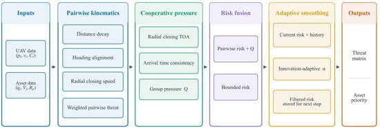
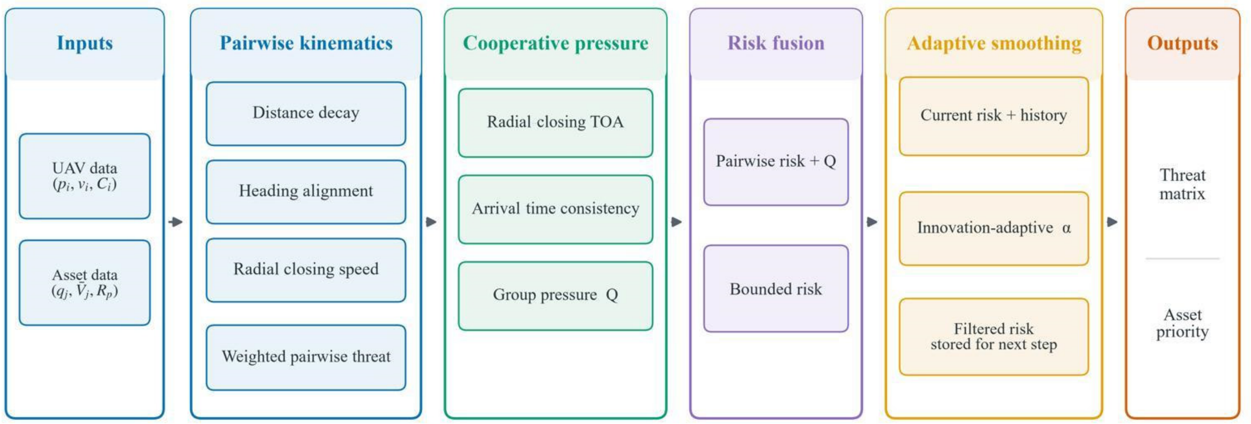
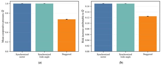
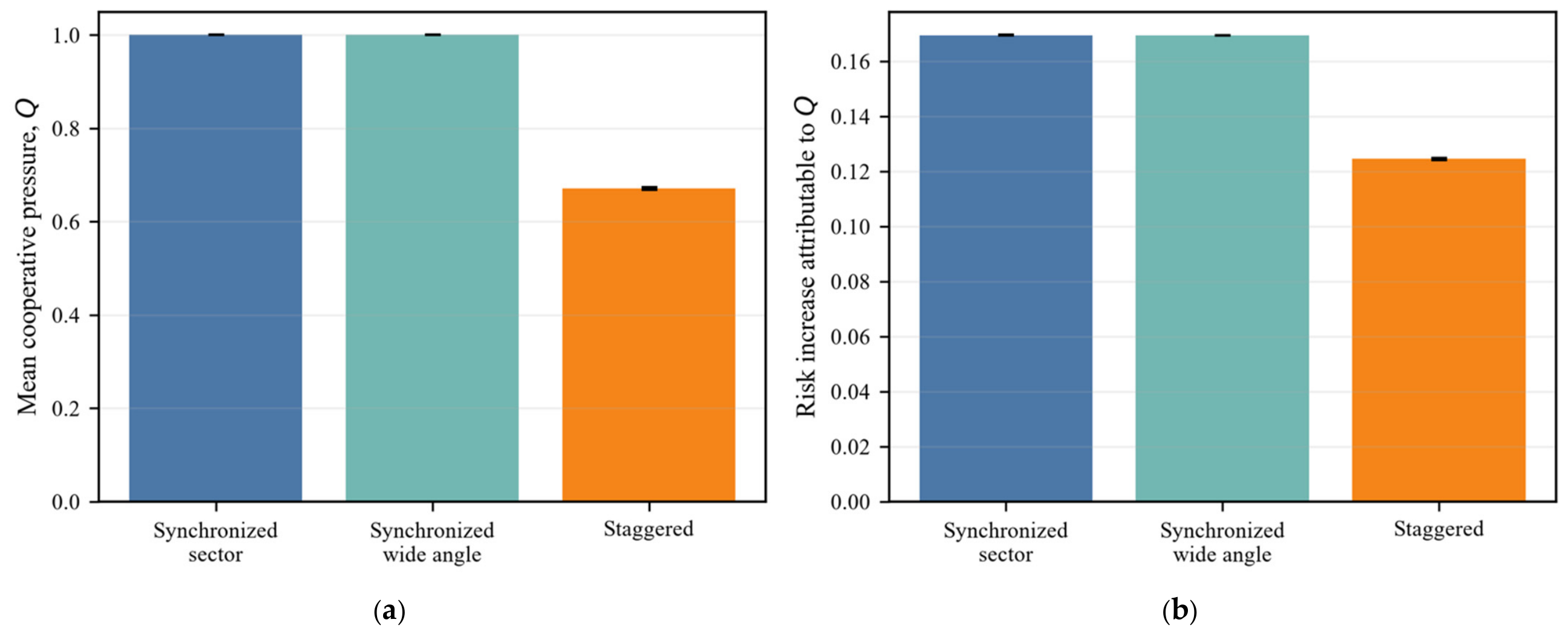
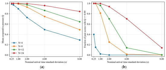
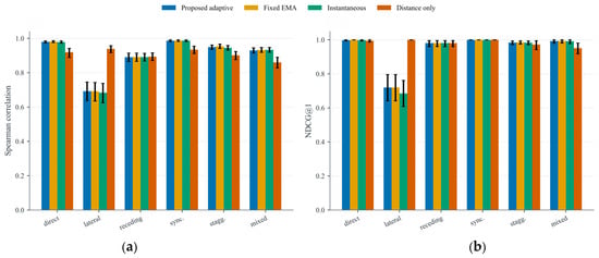
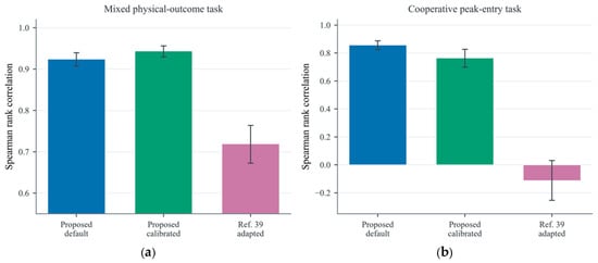
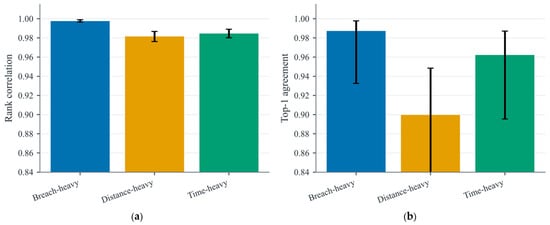
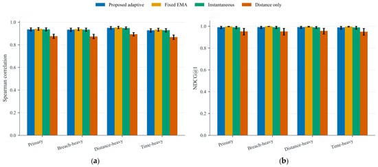
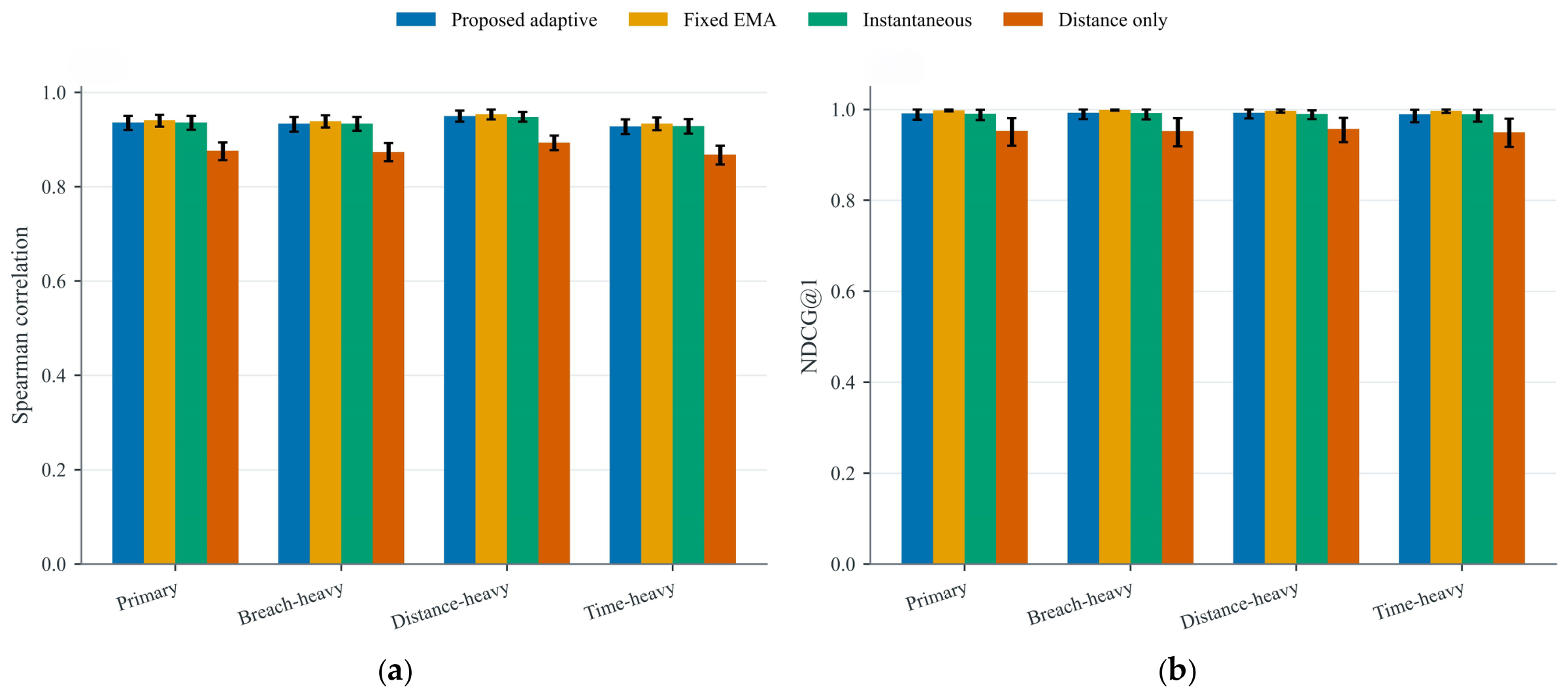
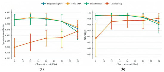
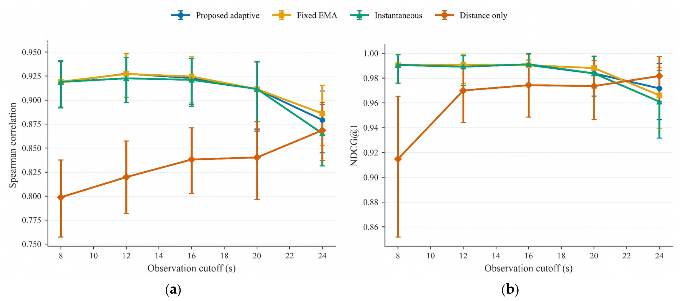
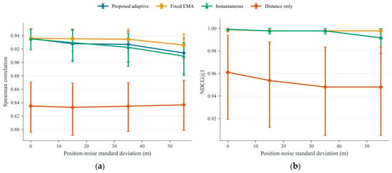
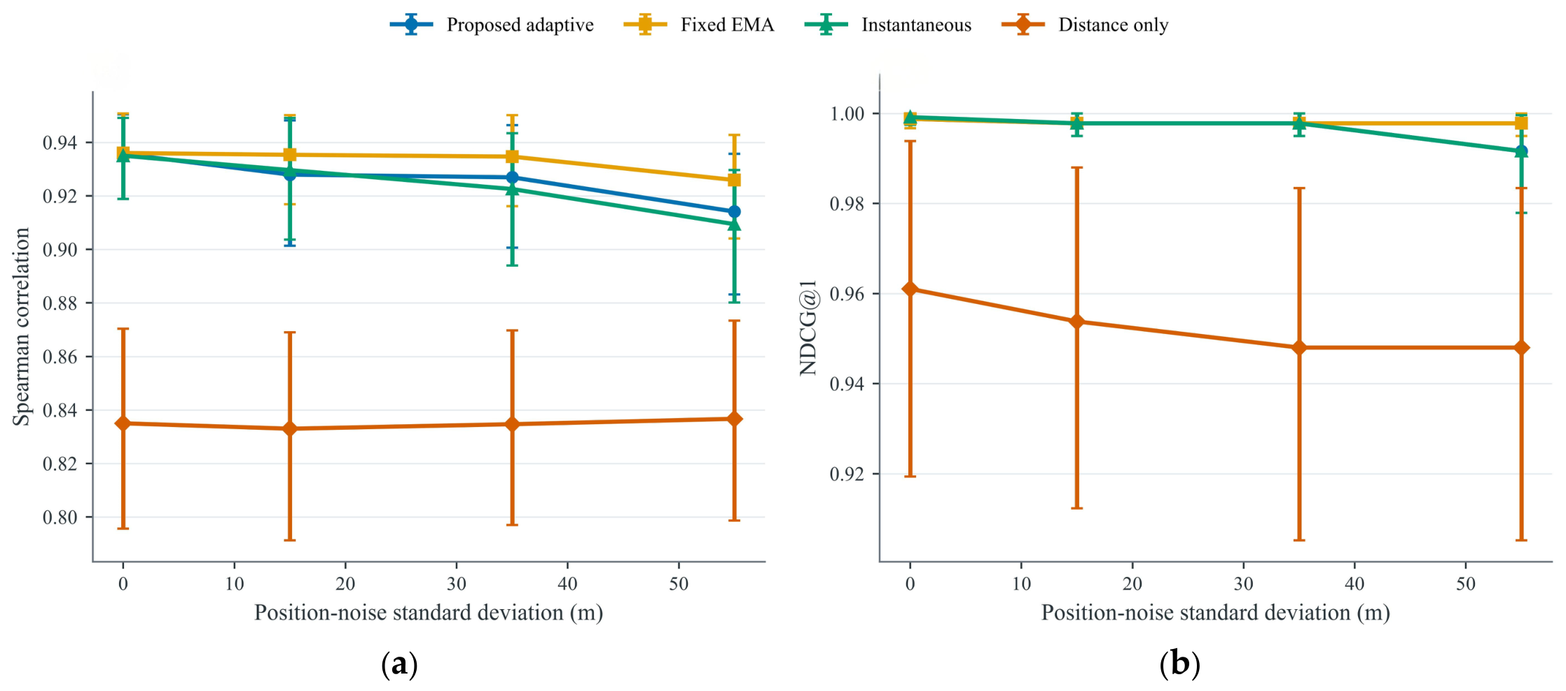
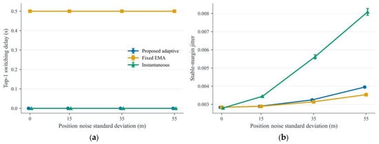
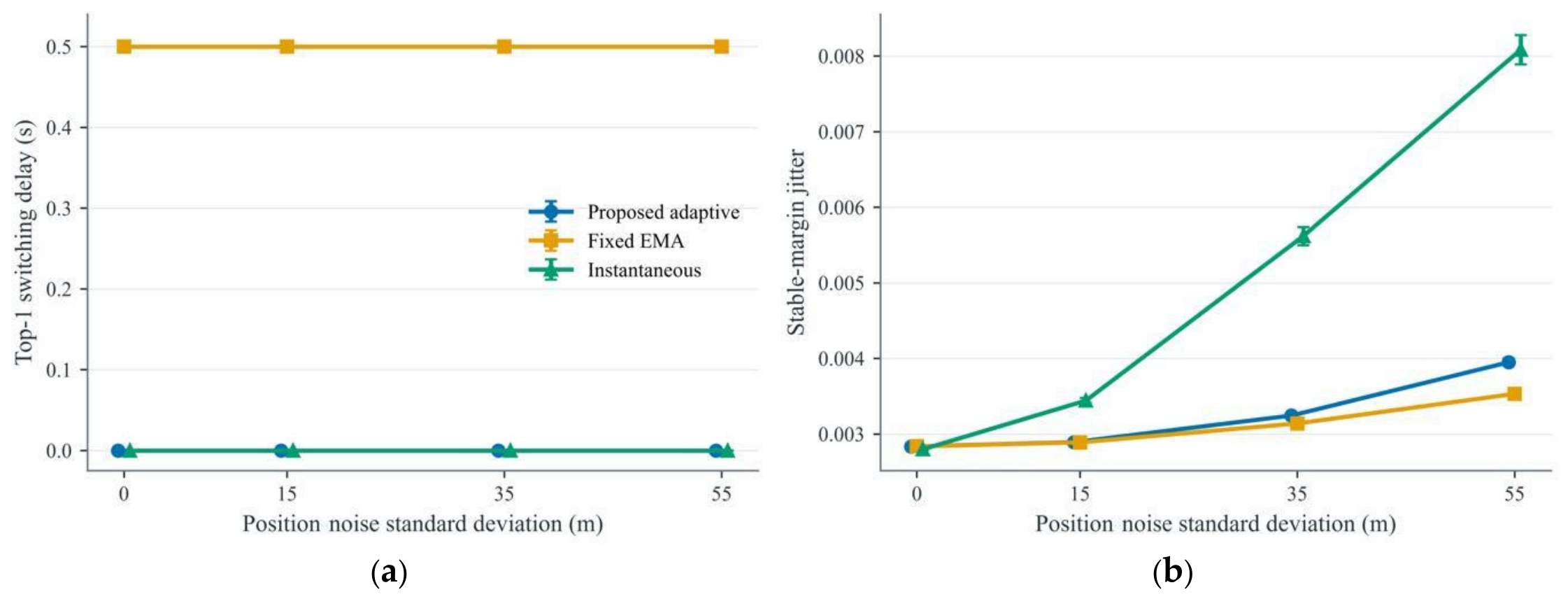
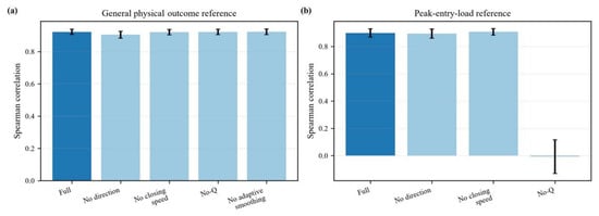
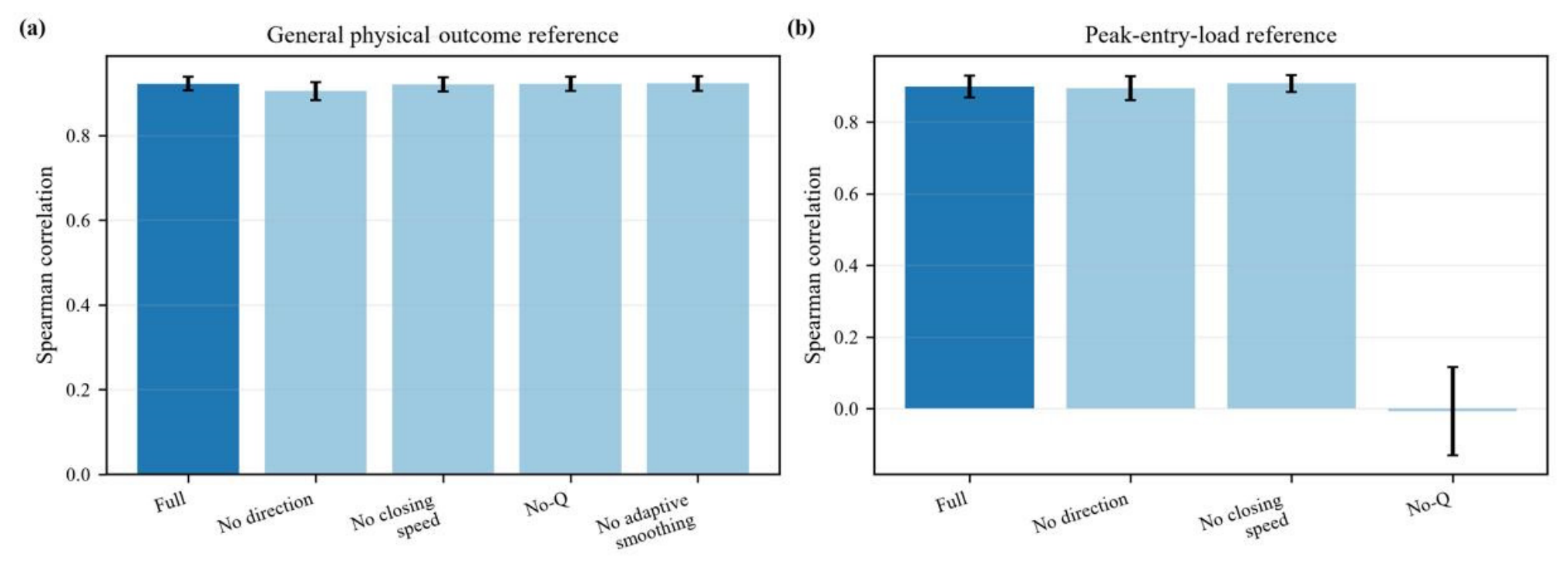
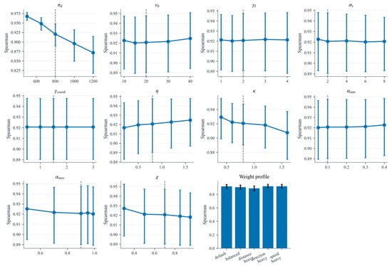
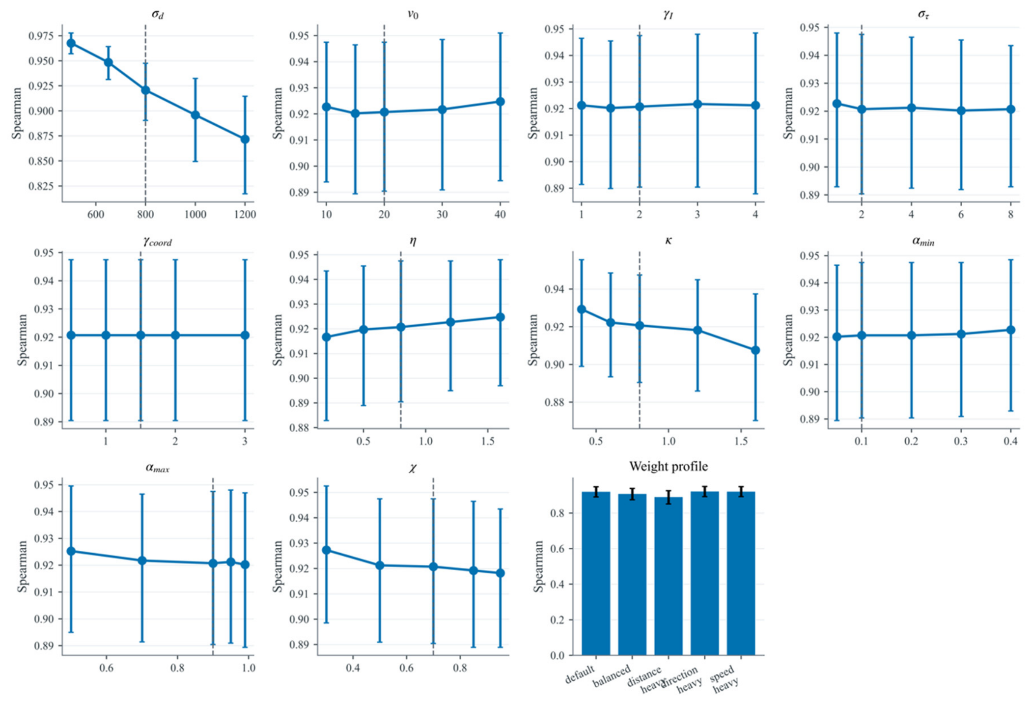
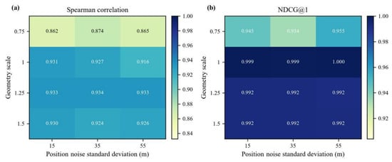
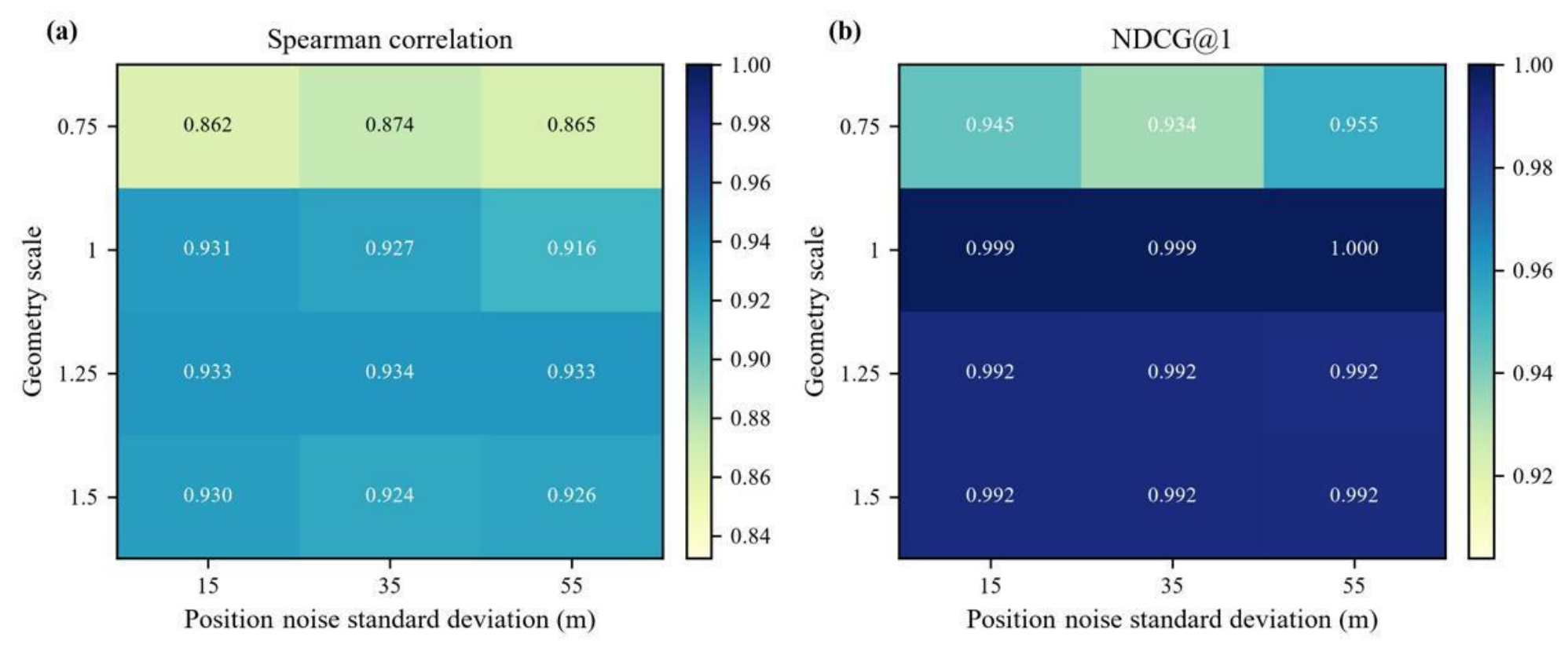
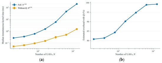
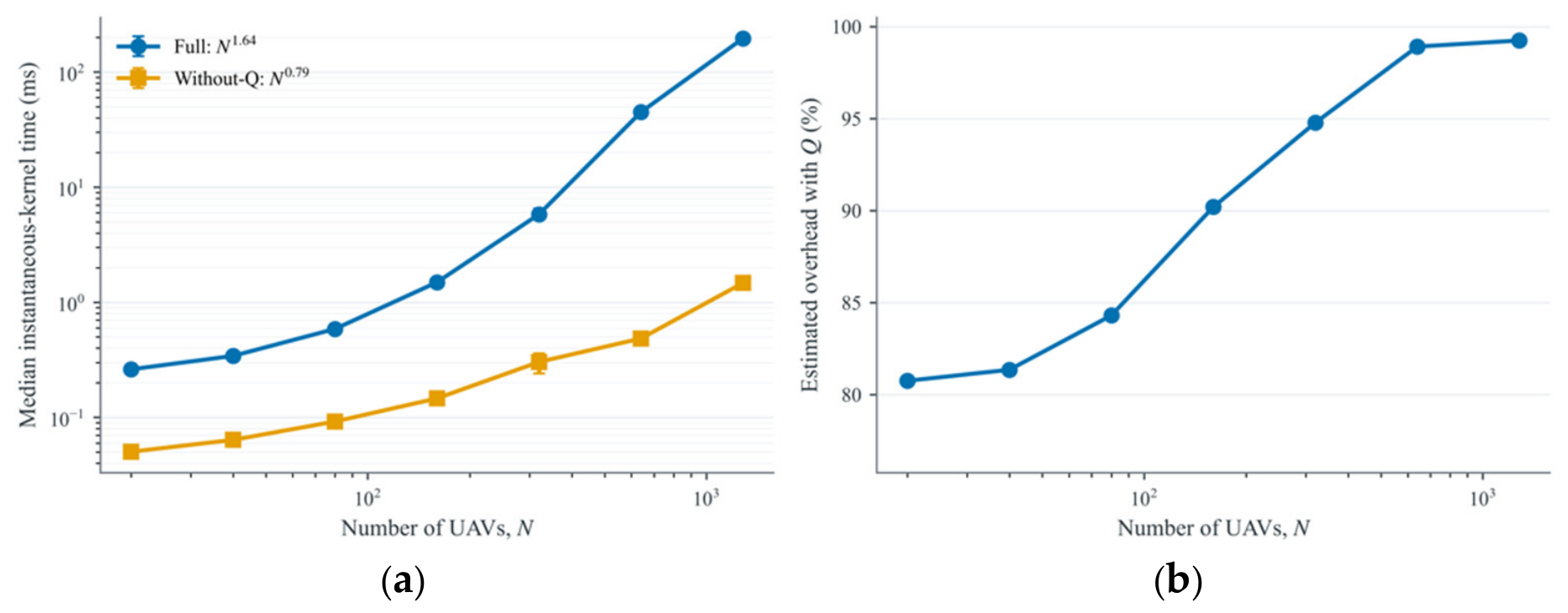

Disclaimer/Publisher’s Note: The statements, opinions and data contained in all publications are solely those of the individual author(s) and contributor(s) and not of MDPI and/or the editor(s). MDPI and/or the editor(s) disclaim responsibility for any injury to people or property resulting from any ideas, methods, instructions or products referred to in the content. |
© 2026 by the authors. Licensee MDPI, Basel, Switzerland. This article is an open access article distributed under the terms and conditions of the Creative Commons Attribution (CC BY) license.