


Highlights
What are the main findings?
- H-MAPPO-LSTM enables hierarchical cooperation among firefighting UAVs.
- It outperforms conventional and flat reinforcement-learning methods.
What are the implications of the main findings?
- Hierarchical planning improves coordination and adaptability.
- The framework supports scalable, real-time wildfire response.
Abstract
Cooperative task planning for amphibious firefighting UAVs deployed across multiple bases is challenging because of complex resource coupling, evolving fire conditions, and real-time decision requirements. This study proposes an H-MAPPO-LSTM method with a three-level hierarchical multi-agent structure: a Command-Center Agent performs global situation assessment and macroscopic task allocation, Base Agents manage UAV resources and decompose regional tasks, and UAV Agents execute water collection, flight, water-dropping, and return operations. LSTM networks are incorporated into the policy networks and combined with PPO and centralized training with decentralized execution to enable multilevel cooperative learning and online dynamic replanning. During deployment, network parameters remain fixed, while online policy inference, real-time decision-making, and dynamic replanning respond to fire-scene changes. The model jointly considers UAV bases, amphibious firefighting UAVs, natural water sources, dynamic fire hotspots, and their constraints. Compared with Flat MAPPO in the static benchmark, H-MAPPO-LSTM reduces mission completion time by 20.2%, average response time by 14.7%, final burned area by 29.7%, and comprehensive cost by 26.0%. Fire-containment rates reach 88% in highly dynamic scenarios and 81.96% in large-scale scenarios. Ablation results indicate that the hierarchical architecture provides the most pronounced contribution under the tested settings, while LSTM, the level-specific centralized critics, and hierarchical rewards provide additional performance contributions under the tested settings.
1. Introduction
Wildfire risk is intensifying in many regions under combined climatic, ecological, and societal pressures. More frequent extreme fire-weather conditions interact with vegetation and landscape factors, while population growth and expansion of the wildland–urban interface increase human-caused ignition pressure and the exposure of people and infrastructure [1,2]. In recent years, amphibious firefighting unmanned aerial vehicles (UAVs) have become important platforms for research on unmanned forest-fire suppression. Wu et al. [3] developed a wildfire-spread and loss-estimation model and optimized the configuration and scheduling of firefighting drones to minimize expected wildfire losses, while Zhu et al. [4] investigated collaborative firefighting strategies for multiple UAV swarms under dynamic fire-spread and resource constraints. General multi-UAV coordination studies have also demonstrated the benefits of cooperative control [5], and wildfire-specific research has shown complementary advantages in distributed-hotspot coverage and resource utilization [4,6,7]. Nevertheless, in large-scale multi-hotspot fires, efficiently coordinating amphibious firefighting UAVs deployed at different UAV bases, planning their water-collection and firefighting routes, and maintaining real-time responsiveness remain a highly complex dynamic decision-making problem.
Cooperative task planning for multi-base amphibious firefighting UAVs in large-scale, multi-hotspot forest fires faces three principal challenges.
- High decision complexity: Task planning must simultaneously process multi-dimensional information on fire conditions (hotspot locations, intensities, and spread trends), available resources (UAV numbers, operational states, and assigned bases), and environmental factors (terrain, meteorology, and accessible water sources). It is therefore difficult to obtain a schedule that balances global efficiency and local feasibility within a limited decision time.
- Low coordination efficiency: Cooperative operations involving multiple UAV bases and UAVs may suffer from imbalanced task allocation, operational conflicts (airspace conflicts and competition for the same water source), and resource waste (duplicated routes and overlapping firefighting effects), thereby reducing overall firefighting efficiency.
- Stringent dynamic-response requirements: Fire conditions evolve continuously, new hotspots may emerge at any time, and UAVs may need to return because of failures or insufficient fuel. Conventional static plans cannot continuously accommodate these changes, making online task adjustment and dynamic replanning necessary.
Existing solution methods for multi-resource cooperative scheduling and task planning can generally be classified into three categories: traditional optimization methods, intelligent optimization algorithms, and multi-agent reinforcement learning (MARL).
Traditional optimization methods commonly use Mixed Integer Linear Programming (MILP) [8], Dynamic Programming (DP) [9], and network-flow models [10] to formulate task assignment, path planning, and resource scheduling in a unified manner. These methods can obtain globally optimal or high-quality approximate solutions when the problem is small and the environment is known and relatively static; surveys of UAV task assignment have also summarized the application of mathematical programming to multi-UAV missions [11]. However, cooperative firefighting with multiple UAV bases involves coupled UAV, base, water-source, and fire-hotspot resources and is constrained by time windows, flight range, water capacity, base capacity, and dynamic fire spread [6,7,12]. As the numbers of UAVs and tasks increase, the search space of the joint optimization problem grows rapidly [7,12,13]. Moreover, when hotspot numbers or fire conditions change, exact optimization methods generally require re-optimization, making it difficult to continuously meet real-time decision requirements in dynamic forest-fire scenarios.
Intelligent optimization algorithms, including Genetic Algorithms (GAs) [14], Particle-Swarm Optimization (PSO) [15], Ant-Colony Optimization (ACO) [16], and Simulated Annealing (SA) [17], are widely applied to UAV task planning and resource scheduling. Through population-based or stochastic search, these algorithms can obtain approximate solutions in complex nonlinear spaces and have been used for multi-UAV mission planning and task assignment [18,19]. However, their solution processes still depend on iterative search and are sensitive to parameter settings and search strategies. When fire conditions change continuously, multiple search iterations generally need to be executed again, and historical decision experience cannot be fully reused; consequently, their response efficiency is limited in continuous online decision-making [20].
Flat Multi-Agent Reinforcement Learning (Flat MARL) can learn cooperative policies through continuous interaction with the environment and is well suited to dynamic decision-making. Deep reinforcement learning has also been applied to UAV maneuver decision-making [21]. Representative MARL methods include MADDPG [22] and MAPPO [23], while value-decomposition alternatives include QMIX [24]. MADDPG follows the Centralized Training with Decentralized Execution (CTDE) paradigm [22], whereas MAPPO extends PPO to cooperative multi-agent settings through decentralized policies and centralized value estimation [23]. However, in multi-base resource scheduling, flat methods usually place UAV bases and UAVs at the same decision level for joint learning. As the number of agents increases, the joint action space may grow rapidly, increasing policy-search difficulty and exacerbating multi-agent non-stationarity and credit assignment [25,26]. Surveys of MARL and resource-allocation applications further identify scalability, coordination, and credit assignment as central challenges [25,27]. In addition, a flat architecture cannot explicitly represent the hierarchical coordination among the command center, UAV bases, and amphibious firefighting UAVs. Hierarchical reinforcement learning and related aerial-mission applications motivate decomposing such long-horizon decisions into subproblems with different temporal scales and decision granularities [28,29,30].
Proximal Policy Optimization (PPO) constrains the magnitude of each policy update by clipping the probability ratio between the current policy and the fixed behavior policy used to collect the current rollout [31]. PPO builds on the trust-region policy-optimization principle while providing a simpler optimization procedure [32]. For cooperative task planning with multiple UAV bases and amphibious firefighting UAVs, PPO can be combined with CTDE and a hierarchical decision structure, enabling agents at different levels to share global information during training while retaining local decision-making capability during execution and thereby adapting to continuously changing fire conditions [23].
Based on the above analysis, this study formulates cooperative task planning for multi-base amphibious firefighting UAVs as a dynamic resource-scheduling problem in a Multi-Agent System (MAS) and proposes an H-MAPPO-LSTM cooperative task-planning model. Following the concept of Hierarchical Reinforcement Learning (HRL) [28] and related hierarchical decision-making applications in complex aerial missions [29,30], the model constructs a three-level command center-UAV base-amphibious firefighting UAV architecture. The command center agent performs global fire-situation assessment and macroscopic task allocation; each Base Agent decomposes macroscopic assignments into specific UAV-hotspot tasks; and each UAV agent selects water sources and executes flight, water collection, water-dropping, and return actions. This architecture decomposes the complex global planning problem into subproblems with different temporal scales and decision granularities. Because fire spread, UAV fuel consumption, and task-execution states exhibit temporal dependence, LSTM networks [33] are incorporated into the policy network at each level to use historical state information for continuous decision-making and dynamic replanning; related aerospace studies also support recurrent modeling of temporally continuous UAV states and trajectories [34,35,36].
Existing HRL and hierarchical MARL methods decompose complex aerial missions into high- and low-level decision processes, but they rarely represent the complete operational chain linking command-level allocation, geographically distributed UAV bases, individual amphibious firefighting UAVs, natural water sources, and dynamically evolving fire hotspots. H-MAPPO-LSTM addresses this limitation through a three-level architecture tailored to multi-base wildfire suppression. The Command Center Agent (CCA) coordinates fire-region allocation across UAV bases, each Base Agent (BA) converts regional objectives into UAV–hotspot assignments, and each UAV Agent (UA) determines the task-execution actions required for water collection, flight, water delivery, and return.
Under the CTDE framework, the proposed method combines role-specific recurrent policies, hierarchical rewards, and multi-timescale decision-making to coordinate global allocation, regional resource management, and UAV-level execution. During deployment, updated observations and retained LSTM states support continuous task adjustment and dynamic replanning without online retraining. These features distinguish H-MAPPO-LSTM from generic hierarchical decompositions and provide a unified framework for cooperative wildfire suppression by multi-base amphibious firefighting UAVs.
The remainder of this paper is organized as follows. Section 2 formally describes cooperative firefighting by multiple UAV bases and multiple UAVs and establishes a mathematical model with optimization objectives and operational constraints. Section 3 presents the three-level agent architecture, including the dimensions and physical meanings of the state and action spaces and the interactions between levels. Section 4 introduces the H-MAPPO-LSTM network, the CTDE training paradigm, the LSTM-based decision process, and the training and deployment pseudocode. Section 5 evaluates the model through static performance comparisons, dynamic robustness experiments, scalability tests, and ablation studies. Section 6 concludes the paper.
2. Problem Description and Mathematical Formulation
This section formally describes and mathematically formulates the cooperative task-planning problem for amphibious firefighting UAVs. The problem is a multi-objective resource-scheduling optimization problem in a dynamic and uncertain environment subject to multiple physical and logical constraints. In this paper, an amphibious firefighting UAV denotes an idealized unmanned water-scooping platform capable of carrying water, accessing a designated water source, performing an abstracted water-scooping operation, dropping water, and returning to a UAV base. Its operational characteristics are represented by water capacity, fuel capacity, cruising speed, fuel-consumption rate, and water-collection rate.
Accordingly, water delivery is modeled as a reduction in hotspot intensity for task-planning evaluation, representing initial attack on discrete spot or surface-fire hotspots and local fire-intensity control rather than direct suppression of a fully developed crown fire. In dense canopies and high-intensity fires, aerial-drop effectiveness is governed by canopy interception, wind, release conditions, and coordination with ground suppression [37]. At the mission-planning level considered here, these operational effects are incorporated through the hotspot-intensity response to each water-delivery action.
2.1. System Components
The entire task system is composed of four fundamental component sets, whose attributes are defined as follows.
- Amphibious Firefighting UAVs Set ()
Where denotes the -th amphibious firefighting UAV and is the total number of UAVs. Each UAV is characterized by the following operational attributes: : maximum water-carrying capacity (kg); : maximum fuel capacity (kg); : average cruising speed (km/h); : fuel consumption rate per unit flight distance (kg/km); : water-collection rate per unit time (kg/s); : index of the assigned UAV base.
- 2.
- UAV base Set ()
Let
where denotes the -th UAV base and is the total number of UAV bases. The attributes of each UAV base include: two-dimensional geographical coordinates of the UAV base; : the set of UAVs stationed at UAV base , satisfying
- 3.
- Fire Hotspot Set ()
Let
where denotes the -th fire hotspot to be suppressed and is the total number of fire hotspots. The attributes of each hotspot are dynamically updated at every time step : : geographical coordinates of the hotspot center at time step ; : fire intensity at time step , representing the total amount of water required to suppress the hotspot. The fire intensity increases as the fire spreads over time and decreases after water is delivered; : static priority of the hotspot, determined according to its proximity to residential areas, critical infrastructure, or ecologically sensitive regions. The priority ranges from 1 to 10, where a larger value indicates a higher suppression priority.
- 4.
- Natural Water Source Set ()
Let
where denotes the -th natural water source (e.g., lakes or reservoirs) available for water collection by amphibious firefighting UAVs, and is the total number of available water sources. Each water source is characterized by : two-dimensional geographical coordinates of the water source; : accessibility and safety evaluation index of the water source, which comprehensively considers factors such as water surface area, water depth, surrounding obstacles, and terrain conditions. The value of ranges from 0 to 1, where a larger value indicates lower water-scooping risk and higher operational efficiency.
2.2. Decision Variables
The objective of cooperative task planning is to generate a decision scheme specifying which UAV performs each task, when it performs the task, and where the task is executed. The core decision variables are defined as follows.
- : equals 1 if UAV is assigned to suppress fire hotspot at time step ; otherwise, it equals 0.
- : equals 1 if UAV is assigned to travel to water source for water scooping at time step ; otherwise, it equals 0.
- : equals 1 if UAV is instructed to return to UAV base for refueling or maintenance at time step ; otherwise, it equals 0.
- : the complete task sequence of UAV Sat time step , expressed as
The objective of task planning is to determine an optimal policy function that generates a conflict-free and efficient decision sequence for all UAVs according to the current system state at each time step.
2.3. Optimization Objectives
The cooperative firefighting task-planning problem for amphibious firefighting UAVs is formulated as a typical multi-objective optimization problem. A weighted-sum approach is adopted to transform multiple objectives into a single optimization objective. The overall objective is to minimize the comprehensive cost :
where , , and denote the weighting coefficients of the three objectives. These coefficients are determined using the Analytic Hierarchy Process (AHP) in conjunction with the priority requirements of emergency response missions.
The AHP criteria are ordered as task-completion time, cumulative fire loss, and propulsion-fuel consumption. Accordingly, the criterion-level pairwise-comparison matrix is defined as , indicating that task-completion time and cumulative fire loss are considered equally important and that each is slightly more important than fuel consumption in emergency operations. This matrix reflects the modeling judgment adopted in the present study rather than judgments derived from an independent expert survey. Normalization of the principal eigenvector yields the weight vector . The maximum eigenvalue is 3.000; therefore, . Using for a three-criterion matrix gives , confirming that the judgment matrix satisfies the standard AHP consistency requirement. The same weights are applied to all methods in the comparative experiments; thus, they represent a common evaluation preference rather than an algorithm-specific advantage.
The individual objective functions are defined as follows.
- Minimization of Task Completion Time )
This objective evaluates the emergency response efficiency and is defined as the time when the intensity of the last remaining fire hotspot decreases below the predefined safety threshold:
where . Here is the number of executed decision steps, s is the decision time interval of the system, and denotes the safety threshold of fire intensity.
In this study, the fire-containment rate is defined as the percentage reduction in aggregate fire intensity relative to its initial value, calculated as 100 × (1 − current aggregate fire intensity/initial aggregate fire intensity) and clipped to the range of 0–100%. A hotspot is regarded as inactive when its intensity is no greater than the safety threshold of 100. An episode terminates when all hotspots are inactive or when the maximum number of simulation steps is reached.
- 2.
- Minimization of Total Fire Loss ()
This objective aims to limit wildfire propagation and reduce the cumulative fire damage throughout the suppression process. It is defined as the accumulated fire intensity of all hotspots over the entire firefighting period:
Here, denotes the intensity of fire hotspot after the state update at decision step.
- 3.
- Minimization of Resource Consumption Cost ()
This objective measures propulsion-fuel consumption during mission execution. In the present simulation, water is obtained from natural water sources and no separately priced suppressant or foam inventory is modeled. Therefore, the resource-cost term includes fuel consumption only and is defined as the total fuel consumed by all UAVs throughout the mission:
where denotes the fuel consumption of UAV at time step , which is calculated according to the flight distance and the corresponding fuel consumption rate per unit flight distance. The division by 1000 converts the accumulated fuel consumption from kilograms to tons.
2.4. Constraints
The task-planning scheme is subject to the following physical and operational constraints.
- UAV Capability Constraints
Fuel-capacity constraint: The remaining fuel of each UAV must remain non-negative throughout the mission, and the total fuel consumption during a single sortie shall not exceed the maximum available fuel capacity:
where denotes the remaining fuel of UAV at time step , and kg represents the minimum fuel reserve required for a safe return to the assigned UAV base.
The return-to-base action includes the fuel consumed during the return flight. Upon arrival at the assigned UAV base, refueling is represented as an instantaneous boundary-state reset between sorties: the UAV fuel state is restored to its maximum capacity before a subsequent dispatch. At the mission-planning level, refueling is implemented as the sortie-boundary fuel-state reset described above. The scheduling state therefore tracks airborne fuel consumption and post-return availability, while the reset links consecutive sorties without introducing a separate ground-service stage.
Water capacity constraint: The onboard water carried by a UAV shall never exceed its maximum water-carrying capacity:
Task exclusiveness constraint: at any time step, each UAV is allowed to perform at most one primary task:
- 2.
- Water-Source Constraints
Accessibility constraint: A UAV is permitted to perform water collection only when the safety assessment value of the selected water source exceeds the predefined threshold:
Water-collection time constraint: The water-collection time depends on the required refill amount and the corresponding water-collection rate:
- 3.
- Mission-Logic Constraints
Fire-suppression prerequisite: A UAV is allowed to execute a firefighting task only when it carries sufficient onboard water:
Task sequence constraint: The typical mission sequence follows the order: .
Unless special missions (e.g., reconnaissance or UAV repositioning) are required, a UAV is prohibited from flying directly to a fire hotspot without first completing a water-collection operation.
- 4.
- Coordination and Safety Constraints
Airspace conflict-avoidance constraint: The three-dimensional distance between any two UAVs shall always remain greater than or equal to the prescribed minimum safety separation:
where denotes the three-dimensional position of UAVs at time step .
Resource allocation uniqueness constraint: Under normal operating conditions, each fire hotspot is assigned to at most one UAV at any given time to avoid redundant resource allocation:
This constraint may be relaxed according to the fire intensity and tactical requirements.
- 5.
- Wildfire Dynamic Constraints
Wildfire-propagation model: The natural evolution of fire intensity is modeled using a cellular automaton:
When fire spreading is enabled, the cellular automaton updates each active hotspot once per simulation step, with s. For hotspot , the spread probability is calculated as
where is the wind speed in m/s, is the terrain slope in degrees, and . A random variable is independently sampled for each active hotspot. If , the fire intensity and burned area are updated as and , respectively; otherwise, both remain unchanged. A hotspot is considered active when , whereas a hotspot at or below this threshold no longer propagates. Wind direction is maintained by the simulator and passed to the fire-spread routine but does not enter the scalar spread-probability calculation, while humidity is not explicitly modeled. Fire spreading is enabled in the dynamic robustness scenarios and the static benchmark and disabled in the default small, medium, and large scenarios.
Fire suppression model: After water is released by a UAV, the fire intensity decreases according to the water delivery effectiveness coefficient:
where denotes the water-delivery effectiveness coefficient, and is the amount of water released during the current firefighting operation.
Following the execution of a water-drop action, the immediate post-drop intensity of hotspot is calculated as
where denotes the fire intensity after water delivery and before the subsequent fire-spread update within the same simulation step, is the amount of water delivered in kg, and is the water-delivery effectiveness coefficient. With the modeled maximum water capacity of 3000 kg, a full-load drop reduces the fire intensity by 2400 units. Therefore, a hotspot with a pre-drop intensity of reaches the safety condition after one full-load drop and does not undergo the subsequent propagation update. Hotspots remaining above the safety threshold are subsequently updated according to the fire-spread rule. All compared methods use the same suppression rule and environment configuration in each corresponding experiment.
- 6.
- Event-Driven Replanning Conditions
To characterize major changes requiring extraordinary resource reallocation, the event-trigger indicator is defined as
where denotes the set of newly emerging fire hotspots at time , is the intensity of hotspot , is the failure indicator of UAV , and is the set of operational UAVs. The thresholds are set to intensity units and . Thus, when at least one newly emerging hotspot exceeds 3000 units, a UAV failure is detected, or the remaining-fuel ratio of an operational UAV falls below 20%.
The hotspot-intensity threshold is determined according to the modeled suppression capability of a single UAV sortie. With the maximum water capacity kg and the water-delivery effectiveness coefficient , one full-load delivery reduces hotspot intensity by units. Considering the extinguishment threshold , the theoretical single-sortie suppression limit is
The replanning threshold is set above this limit so that extraordinary replanning is activated for a newly emerging hotspot that clearly requires multiple water-delivery operations and may change the inter-base resource allocation. Newly emerging hotspots with intensities not exceeding 3000 units remain available to the agents but are handled through the regular decision schedule.
The remaining-fuel ratio is used as an early-warning threshold for event-triggered replanning and return-to-base decision-making. Under the benchmark configuration, it corresponds to 600 kg of fuel. By contrast, kg is the minimum safety reserve that must be preserved for the return flight. The early-warning threshold is therefore activated before the minimum reserve is reached, providing sufficient time for task reallocation and safe return.
The above mathematical formulation indicates that the cooperative firefighting task-planning problem for amphibious firefighting UAVs is a large-scale, nonlinear, multi-objective dynamic optimization problem characterized by path dependency and combinatorial complexity. Conventional optimization approaches are generally unable to generate high-quality solutions within the stringent time constraints required for emergency response, particularly in dynamic replanning scenarios. Therefore, a hierarchical multi-agent reinforcement learning framework based on Proximal-Policy Optimization (PPO) provides an effective solution to this problem.
3. Hierarchical Multi-Agent Reinforcement Learning Framework
To effectively solve the above cooperative task-planning problem, a hierarchical multi-agent reinforcement learning (HMARL) framework is proposed. The framework maps the real-world command-and-control hierarchy into a three-level multi-agent architecture and is trained under the Centralized Training with Decentralized Execution (CTDE) paradigm.
3.1. Three-Level Multi-Agent Architecture
The proposed framework decomposes the global cooperative task-planning problem into three hierarchical decision-making levels, each managed by an agent type with distinct responsibilities. The decision intervals are determined using a nested temporal scheme based on the simulation step s and the decision scope of each level. Because the UAV state, including its position, fuel, water load, and task status, is updated at every simulation step, the UA makes a decision every step, giving s. The BA updates its UAV–hotspot allocation after two UA execution steps, giving s, so that each allocation decision incorporates recent UAV execution feedback while maintaining task continuity. The CCA updates the global fire-to-base allocation after three BA decision cycles, giving s, which allows global assignments to be adjusted using aggregated lower-level feedback without excessive reassignment. Thus, the update factors are , and the three levels are synchronized every s. Between two decision instants, the most recent upper-level command remains active, allowing the lower-level agents to continue execution without interruption. This multi-timescale mechanism balances responsiveness and task continuity and provides the temporal basis for the three-layer architecture described below.
- Top Level: Command Center Agent (CCA)
The CCA serves as the global strategic commander and maintains a global view of the wildfire situation and all available resources. Leveraging this comprehensive situational awareness, it partitions the entire wildfire region into multiple subregions and assigns these subregions, or clusters of fire hotspots, to different Base Agents as high-level mission objectives. Its primary objective is to maximize overall firefighting effectiveness while maintaining balanced resource utilization among UAV bases.
- 2.
- Middle Level: Base Agent (BA)
Each UAV base is associated with an independent Base Agent, which acts as the regional tactical commander. After receiving high-level mission objectives from the CCA, the BA performs tactical task allocation within its managed UAV fleet. Specifically, it determines which UAVs should be dispatched, when they should be dispatched, and which fire hotspot it should suppress, thereby translating strategic objectives into executable mission commands.
- 3.
- Bottom Level: UAV Agent (UA)
Each amphibious firefighting UAV is associated with an independent UAV Agent that functions as the mission executor.
Upon receiving task assignments from its corresponding BA, the UA autonomously plans and executes the required sequence of low-level actions. These actions include selecting an appropriate water source, planning the flight trajectory, performing water-collection and water-delivery operations, and deciding whether to return to the assigned UAV base according to its current operational status.
The decision boundary among the three levels is defined by their decision objects and temporal scales. The CCA allocates fire hotspots or fire regions to UAV bases every 60 s without selecting individual UAVs or execution actions. Each BA converts these regional assignments into specific UAV–hotspot assignments every 20 s. Each UA then selects water sources and updates its task-execution macro-actions every 10 s according to the assigned hotspot and its local state, but it cannot independently change the hotspot assigned by the BA.
The proposed hierarchical architecture offers three major advantages.
- First, it reduces decision-making complexity by decomposing a large flat decision space into multiple hierarchical subproblems that are easier to solve.
- Second, it improves learning efficiency, as high-level agents provide meaningful subgoals that guide the exploration of lower-level agents, thereby accelerating policy convergence.
- Third, it enhances interpretability and robustness. The hierarchical decision-making process closely resembles real-world command-and-control structures, allowing higher-level agents to rapidly replan missions when lower-level agents fail to execute assigned tasks, thereby preventing the collapse of the entire system.
3.2. Quantitative Definition of the State and Action Spaces
To ensure the trainability and deployability of the framework, the state and action spaces of all three hierarchical agents are quantitatively defined, including the physical meaning, encoding, padding, and masking rules of every feature group.
Continuous state variables are primarily scale-normalized. Ordered discrete variables, such as mission phases, are represented using scalar codes, whereas unordered categorical variables, such as UAV-base affiliation, are represented using One-Hot encoding. Binary variables, such as target-validity indicators, are encoded using 0–1 indicators. Depending on their physical meanings, some relative-position and fire-intensity features are not strictly bounded within [0, 1]. The specific encoding of each feature is provided in the corresponding state-space definition.
Fixed-dimensional entity-slot encoding is used at all three levels. Let , , and denote the maximum numbers of fire hotspots (or aggregated fire regions), UAV bases, UAVs, and water sources represented in the CCA observation, respectively. For BA , , , and denote the maximum numbers of assigned fire hotspots, managed UAVs, and local water sources; for a UA, and denote the maximum numbers of perceived water sources and neighboring UAVs. Valid entities are placed in deterministic slots, unused slots are zero-padded, and binary validity masks prevent padded entities from contributing to attention, pooling, or action selection. Fire entities are ordered by descending priority and intensity and then by ascending distance; UAVs are ordered by availability, remaining fuel, and distance; water sources and neighboring UAVs are ordered by distance. The masks are auxiliary variables and are not counted in the reported input dimensions. The numerical capacities used in the benchmark are specified in the experimental configuration.
3.2.1. Command-Center Agent (CCA)
As the global strategic decision-maker, the Command-Center Agent (CCA) maintains a global view of the entire system. Its state space contains macroscopic information of the wildfire environment and available resources, while its action space performs high-level task allocation between fire hotspots and UAV bases.
- State Space ()
The total dimensionality of the CCA state space is under the benchmark configuration. The five terms represent the global wildfire situation, UAV-base resources, UAV status, water-source distribution, and mission-time information, respectively. In particular, each UAV-status entry contains an M-dimensional One-Hot vector identifying its assigned UAV base, its two-dimensional position, and its mission-status code. Fuel and water availability required for tactical allocation are summarized at the BA level rather than expanded in the CCA vector. Table 1 summarizes the features and dimensions of the CCA state space.
Table 1.
Definition of the CCA state space.
- 2.
- Action Space ()
The CCA assigns each fire hotspot to a designated UAV base using a discrete fire hotspot–UAV-base assignment representation. The total action dimension is under the benchmark configuration. Table 2 summarizes the CCA action-space representation.
Table 2.
Definition of the CCA action space.
When the actual number of fire hotspots exceeds , the hotspots are first clustered into groups using the K-means algorithm, and task allocation is subsequently performed at the cluster level.
3.2.2. Base Agent (BA)
Each Base Agent (BA) functions as a regional tactical decision-maker. It receives only the local mission objectives assigned by the CCA together with the resource information within its jurisdiction. Its action space performs tactical task allocation between UAVs and fire hotspots.
- State Space ()
For , the state dimension is under the benchmark configuration. The four terms correspond to assigned fire hotspots, managed UAVs, local water sources, and UAV-base status, respectively. Table 3 summarizes the features and dimensions of the BA state space.
Table 3.
Definition of the state space.
- 2.
- Action Space ()
The assigns one available UAV to one pending fire hotspot. The total action dimension is under the benchmark configuration. Table 4 summarizes the BA action-space representation.
Table 4.
Definition of the action space.
If no idle UAVs or pending fire hotspot is available, the BA outputs a null action and waits until the next decision interval.
3.2.3. UAV Agent (UA)
Each UAV Agent (UA) serves as the mission executor and receives a BA mission command together with local sensor information. Its observation uses local candidate slots rather than the full global resource set: up to water sources and J neighboring UAVs. The general state dimension is = 3 + 8 + 4 + 3J = 29 under the benchmark configuration. This representation reduces the amount of global information processed directly by an individual UA.
- State Space ()
For the -th UAV Agent, the total state dimension is fixed at 29. Table 5 summarizes the features and dimensions of the UA state space.
Table 5.
Definition of the state space.
- 2.
- Action Space ()
The executes five categories of discrete macro-actions. The action corresponding to traveling toward a water source additionally contains a water-source selection parameter. The total action dimension is , under the benchmark configuration. Table 6 summarizes the UA action categories, trigger conditions, and decision intervals.
Table 6.
Definition of the action space.
The macro-action category is represented using a five-dimensional One-Hot vector. The water-source selection parameter is effective only when the Navigate to a Selected Water Source action is selected; otherwise, all water-source selection variables are set to zero.
In this study, the amphibious firefighting UAV is modeled as an unmanned fixed-wing amphibious aircraft with water-scooping capability, referring to the operational mode of the existing amphibious firefighting aircraft. At the mission-planning level, its main characteristics are described by water capacity, fuel capacity, cruising speed, fuel-consumption rate, and water-collection rate. When performing a water-collection task, the UAV flies to the selected water source and then performs water scooping, which in practice involves approach, water-surface contact, scooping while skimming on the water, and departure. Since this study focuses on cooperative multi-UAV task planning rather than detailed hydrodynamics and flight dynamics, the process is simplified as water collection at a predefined rate until the onboard water tank is full.
3.3. Interactions Among Hierarchical Agents
The proposed H-MAPPO-LSTM framework follows the Centralized Training with Decentralized Execution (CTDE) paradigm. Consequently, the interaction mechanisms during execution differ significantly from those during training. Since the three types of agents operate at different decision intervals, an asynchronous interaction mechanism is naturally established, namely CCA (1 min) → BA (20 s) → UA (10 s). High-level agents provide decision guidance for lower-level agents, whereas feedback from lower-level agents enables higher-level agents to perform dynamic replanning.
3.3.1. Interaction During Execution (Decentralized Execution)
During execution, no centralized controller is involved. Each agent interacts only through hierarchical task commands and state feedback, thereby maintaining low decision latency and satisfying the real-time requirements of emergency wildfire response. Table 7 summarizes the information exchanged among agents during execution.
Table 7.
Interaction relationships during the execution stage.
The complete execution procedure is summarized as follows.
- Global situation update: The global situation awareness system collects the system state every 10 s and synchronizes the updated information to all agents.
- Strategic decision-making by the CCA: Every 1 min, the CCA generates fire hotspot–UAV base assignment decisions according to the latest global state and broadcasts them to all BAs.
- Tactical decision-making by the BA: Every 20 s, each BA generates UAV–hotspot assignments from the latest CCA command, the state feedback of its managed UAs, and local environmental information, and dispatches tasks to available UAVs.
- Mission execution by the UA: Every 10 s, each UA determines its macro-action according to the assigned mission and locally perceived information, executes the corresponding operation, and continuously reports its state to the associated BA.
- Hierarchical state feedback: Each BA collects the state information of all managed UAs and summarizes it every 1 min before reporting it to the CCA. The CCA uses the reports from all BAs to update the global resource state for the next strategic decision.
- Dynamic replanning: Under normal conditions, when a new fire hotspot emerges, its state is immediately incorporated into the observations and processed by the hierarchical policies at their corresponding decision times. When an emergency event defined in Section 2.4 is detected, the CCA immediately performs a one-time event-driven strategic update, while the BA decision interval is temporarily reduced from 20 s to 10 s. After this event-driven update, the CCA and BAs resume their regular decision intervals.
- Interlevel conflict resolution: UAVs that are unavailable or do not satisfy the operational constraints are excluded from candidate actions through action masking. If a BA has no feasible UAV for a task assigned by the CCA, it outputs a null action and reports the updated resource state, allowing the CCA to reassign the task rather than forcing an infeasible command.
3.3.2. Interaction During Training (Centralized Training)
During training, a centralized value network is introduced to utilize trajectory data collected from all agents. Centralized training can help mitigate the non-stationarity induced by simultaneously learning agents [22,25], while centralized value estimation and counterfactual or decomposed value formulations provide established mechanisms for improving cooperative credit assignment [26,38]. Table 8 summarizes the interactions among agents and training components.
Table 8.
Interaction relationships during the training stage.
The complete training procedure is summarized as follows.
- Trajectory sampling: All agents interact with the simulation environment using the fixed old policies to collect rollout sequences of 200 time steps. The collected trajectories are stored in a current-cycle sequential rollout buffer for subsequent GAE computation and PPO updates. The rollout buffer is cleared after each policy-update cycle before new trajectories are collected.
- Advantage estimation: State-value estimates and Generalized Advantage Estimation (GAE) [39] are computed from the collected current-cycle rollouts using the corresponding level-specific centralized critics. The rollout data are then divided into mini-batches of contiguous trajectory segments with a sequence length of 20 to preserve temporal dependencies during LSTM-based optimization.
- Policy optimization: The hierarchical policy networks are updated by maximizing the PPO-clipped surrogate objective using local observation sequences and the corresponding level-specific GAE advantages. Each mini-batch is optimized for three epochs.
- Value function optimization: The level-specific centralized critics are updated by minimizing the mean squared error (MSE) between the predicted state values and the corresponding return targets. Within each hierarchy, agents share the corresponding centralized critic.
- Policy synchronization: After each training batch, the parameters of the latest policy networks are softly updated to the corresponding old policy networks.
- Hierarchical reward propagation: The global reward generated by the CCA is incorporated into the BA reward with a weighting coefficient of , ensuring that tactical decisions remain aligned with the overall mission objective. The UA reward consists only of local task-completion rewards and efficiency penalties, whereas global coordination is reflected through the advantage estimates produced by the centralized value network.
3.4. LSTM-Based Agent Design
The wildfire-suppression environment is highly dynamic, and task execution exhibits strong temporal continuity. Consequently, agent decision-making should not rely solely on the current observation but should also incorporate historical information and temporal evolution patterns. To this end, a Long Short-Term Memory (LSTM) network is embedded into both the policy network and the value network of each hierarchical agent. Through its gated memory mechanism, LSTM is designed to improve the learning of long-term dependencies and mitigate the vanishing-gradient problem encountered in conventional recurrent neural networks [33,40].
The decision-making process of each LSTM-based agent consists of three sequential stages: feature extraction, temporal encoding, and decision generation.
During the feature extraction stage, each agent receives the observation at decision time step , which is processed by a feature encoder to obtain the feature representation . Specifically, global-wildfire-situation information is encoded using a two-layer Convolutional Neural Network (CNN), while vectorized resource states and environmental information are encoded using a three-layer Multi-Layer Perceptron (MLP).
During the temporal encoding stage, the extracted feature vector , together with the hidden state and cell state from the previous time step, is fed into the LSTM unit to generate the current hidden state and cell state . The hidden state summarizes historical observations and serves as a compact representation of the agent’s understanding of the current operational situation.
During the decision generation stage, the hidden state is forwarded to the output layers of the subsequent policy network (Actor) and value network (Critic) to generate the action probability distribution and state-value estimation, respectively.
By incorporating the LSTM architecture, each agent is capable of memorizing critical historical events, such as previously visited water sources and fuel consumption trends, while simultaneously capturing the temporal evolution of the wildfire environment, including fire propagation patterns. Consequently, the proposed framework enables more foresighted and context-aware decision-making than memoryless policies.
The proposed planner does not rely solely on a previously predicted fire trajectory. When the observed fire intensity or hotspot state differs from the modeled evolution, the updated information is incorporated into the agent observations, allowing the hierarchical policies to adjust subsequent decisions based on the latest fire state. If the deviation satisfies an event-driven replanning condition defined in Section 2.4, an immediate strategic update is triggered. Nevertheless, the LSTM provides temporal information rather than eliminating fire-model error, and substantial deviations beyond the conditions represented during training may still degrade policy performance.
3.5. Reward Function Design for Multi-Agent Reinforcement Learning
This section defines the reward functions for the three hierarchical agents to establish a complete multi-agent reinforcement learning framework. The proposed reward design is fully compatible with the training paradigm of the PPO algorithm.
- Reward Function of the Command-Center Agent (CCA)
The reward of the CCA evaluates the effectiveness of global strategic decision-making and is formulated as
where and are weighting coefficients. The first term penalizes the total wildfire intensity over all fire hotspots, the second term represents the time cost, and the third term penalizes the imbalance of task allocation among UAV bases.
Here, denotes the variance of the workload assigned to different UAV bases, where the workload is jointly determined by the estimated total flight time and the weighted cumulative fire intensity of the assigned fire hotspots. This term encourages balanced resource allocation across the entire system.
- 2.
- Reward Function of the Base Agent (BA)
The BA adopts a hierarchical reward mechanism that simultaneously considers global coordination and local operational efficiency:
where is the weighting coefficient of the global reward, ensuring that the tactical decisions of each BA remain consistent with the overall mission objective.
The local reward is defined as
where and . The first term rewards the reduction in wildfire intensity achieved by the fire hotspots assigned to the -th UAV base, while the second term penalizes the number of idle UAV, encouraging efficient utilization of available resources.
- 3.
- Reward Function of the UAV Agent (UA)
The reward of the UAV Agent consists of four components: task completion reward, efficiency reward, safety penalty, and distance-progress shaping reward.
Task completion reward: A positive reward of is assigned when the UAV successfully delivers water over the designated fire hotspot, while a moderate reward of is granted after successful water collection.
Efficiency reward: A small negative reward,
is imposed during flight, where and . This term encourages UAVs to select fuel-efficient and time-efficient flight trajectories.
Safety penalty: A reward penalty of −50 is applied when the remaining fuel falls below 20% of the maximum fuel capacity. A reward penalty of −1000 is applied if the UAV collides with an obstacle or enters a hazardous area. If both conditions occur at the same decision step, the more severe penalty of −1000 takes precedence.
Distance-progress shaping reward: A distance-progress reward-shaping mechanism is adopted to accelerate policy learning. Specifically, the UAV receives a positive reward of +1 whenever its distance to the assigned fire hotspot is reduced by 1 km, guiding the agent toward the mission objective more efficiently.
4. H-MAPPO-LSTM-Based Cooperative Task-Planning Algorithm
Building upon the hierarchical multi-agent reinforcement learning framework described above, this paper proposes the H-MAPPO-LSTM algorithm for cooperative task planning. The proposed algorithm combines the stable optimization capability of Proximal-Policy Optimization (PPO), the temporal representation capability of Long Short-Term Memory (LSTM) networks, and the complexity reduction achieved by the hierarchical architecture. Consequently, it effectively addresses the non-stationarity and coordination challenges inherent in multi-agent reinforcement learning while naturally supporting online dynamic replanning.
4.1. H-MAPPO-LSTM Framework
The H-MAPPO-LSTM algorithm equips each hierarchical agent with an independent LSTM-based policy network (Actor) and introduces three level-specific centralized state-value critics for the CCA, BA, and UA levels. Agents within the same level share the corresponding critic, while the critics at different levels are trained independently to accommodate their respective decision objectives and temporal scales. The overall framework follows the Centralized Training with Decentralized Execution (CTDE) paradigm. PPO constrains each policy update through a clipped probability ratio, improving training stability while retaining efficient decentralized execution.
- Network Architecture
Policy Network (): Each hierarchical agent is equipped with an independent policy network. The network architecture consists of a feature encoder (CNN/MLP), followed by two LSTM layers with a hidden dimension of 256, two fully connected layers with dimensions 128 and 64, respectively, using ReLU activation, and a Softmax output layer. The input dimensions correspond to the state spaces of the three hierarchical agents, namely 165 for the CCA, 78 for the BA, and 29 for the UA. The output dimensions correspond to their respective action spaces, namely 60, 14, and 10, respectively.
Centralized Value Network (): All agents within the same hierarchy share a global centralized value network. Three such networks are constructed for the CCA, BA, and UA levels, respectively. Each network consists of a global feature encoder (CNN + MLP), followed by two LSTM layers with a hidden dimension of 512, three fully connected layers with dimensions 256, 128, and 64, respectively, using ReLU activation, and a linear output layer. The input dimension equals the concatenation of the global state and the joint actions of all agents within the corresponding hierarchy:
where 165 represents the global state dimension and 202 corresponds to the joint action dimension of all hierarchical agents. Each critic independently outputs a one-dimensional estimate of the value function for its corresponding hierarchical decision process. Although the three critics adopt the same network architecture and centralized input structure, they maintain independent parameters and are trained using their respective hierarchical rewards and value targets.
- 2.
- Core Computation Process
Feature Extraction and Temporal Encoding: Consistent with the use of LSTM for temporal-dependency modeling [33], the local observation of each agent is first encoded into a latent feature representation, which is subsequently processed by the LSTM module together with the hidden state and cell state from the previous time step,
where denotes the local observation of the agent, is the encoded latent feature representation, and represents the hidden state that encodes historical information accumulated during sequential decision-making.
Multi-head policy generation: The LSTM hidden state is mapped to the corresponding masked categorical heads. For the CCA, the joint action log-probability is the sum of the log-probabilities of all valid fire-region heads. For a BA, it is the sum of the selected UAV-head and fire-head log-probabilities. For a UA, it is the macro-action log-probability plus the source-head log-probability only when navigation to water is selected. Actions are sampled independently from the applicable heads and then combined into a structured hierarchical action: .
This factorized representation generates complete structured assignments while preserving tractable categorical distributions and action masking.
Level-Specific Value Estimation: For each hierarchy , the corresponding centralized critic estimates the state value according to
The resulting level-specific state values are aligned with the responsibilities and decision intervals of their respective levels: the CCA critic evaluates global fire-hotspot-to-base allocation over the 60-s strategic decision process, the BA critic evaluates regional UAV-to-hotspot assignment over the 20-s tactical decision process, and the UA critic evaluates UAV-level mission execution at each 10-s decision step. These state values are used with the corresponding hierarchical rewards to compute TD errors and GAE advantages, which guide the policy updates at that hierarchy. Accordingly, the TD errors, GAE advantages, and value targets are calculated separately for the three levels, and each critic is updated using only the learning signals associated with its corresponding hierarchy.
4.2. Centralized Training with Decentralized Execution (CTDE)
In multi-agent environments, the actions of one agent continuously alter the environment perceived by other agents, resulting in the well-known non-stationarity problem during policy learning. The Centralized Training with Decentralized Execution (CTDE) paradigm helps mitigate this issue by exploiting global information during training while allowing agents to make decisions independently during execution. This constitutes the fundamental design principle of the MAPPO algorithm.
During training, the CCA, BA, and UA policies are guided by their corresponding level-specific centralized critics. Each critic receives the 165-dimensional global state and the 202-dimensional fixed-length joint-action encoding available during centralized training. This centralized information helps mitigate non-stationarity and credit-assignment difficulties.
For the proposed three-level architecture, centralized training is performed within each hierarchy, while inter-level coordination is realized through hierarchical reward propagation.
During intra-level training, all agents within the same hierarchy share one critic: all BAs share and all UAs share . The CCA uses . Thus, the framework contains three critics in total rather than one critic per individual agent.
During inter-level coordination, the reward generated by the higher level is incorporated into the lower-level reward as defined in Section 3.5. The three critics are optimized separately using their corresponding hierarchical rewards, aligning tactical and execution-level learning with the global objective.
After training, none of the corresponding level-specific critics participates in decision-making. Each agent selects actions using only its local observation and policy network. The temporal memory provided by LSTM supports the representation of changing flight states and mission environments [33,34,35,36], while the learned hierarchical policies retain cooperative behavior with low decision latency and support online dynamic replanning.
During a temporary communication interruption, the most recent valid upper-level command remains active. If the CCA–BA link is interrupted, the BA continues allocating available UAVs within the most recently assigned fire region based on local information. If the BA–UAV link is interrupted, the UAV continues its current task using the most recent valid assignment and onboard observations. When the task can no longer be executed safely, particularly because of insufficient fuel, the UAV returns to its assigned base.
4.3. H-MAPPO-LSTM Training Procedure and Network Update
The proposed H-MAPPO-LSTM algorithm uses sequential trajectory segments to preserve temporal continuity. For each hierarchy, GAE is computed using the corresponding level-specific critic and reward; the hierarchical policy is optimized with the PPO clipped surrogate objective, and its critic is trained with a separate mean squared-error value loss. Each mini-batch is optimized over multiple epochs.
For each hierarchy l ∈ {CCA, BA, UA}, the temporal-difference error is computed as
The corresponding level-specific advantage is estimated by
Here, is the reward of hierarchy , is its TD error, is the termination indicator ( for a terminal transition and 0 otherwise), is the discount factor, and is the GAE parameter. The CCA, BA, and UA policy losses therefore use separate advantages computed from their respective critics.
The overall training procedure of the proposed H-MAPPO-LSTM algorithm is summarized in Algorithm 1, while the complete pseudocode is provided in Algorithm A1 of the Appendix A.
| Algorithm 1: Overall Training Procedure of H-MAPPO-LSTM |
Output: Trained hierarchical policies 1 Initialize CCA, BA, UA policy networks, centralized critic , , . old policies , rollout buffer , and optimizers. 2 for episode = 1, 2, …, E do 3 Reset the environment and collect trajectories using the fixed old policies. 4 for t = 0, 1, …, T − 1 do 5 Update the CCA action every six steps. 6 Update each BA action every two steps. 7 Update each UA action at every step. 8 Execute the joint hierarchical action . 9 Observe , hierarchical rewards , , and termination flag . 10 Store in trajectory T. 11 if dt then break. 12 end 13 Compute value estimates, GAE advantages, and value targets: 14 Split T into sequences of length Lseq, repeat collection until BatchSize. 15 for epoch = 1, 2, …, Kepoch do 16 Randomly shuffle all sequences in into mini-batches. 17 for each mini-batch in do 18 Update all policy networks using the clipped PPO objective: 19 Update the centralized critics using the value loss. 20 Apply gradient clipping. 21 end 22 end 23 Soft-update old policy parameters: . 24 Clear before the next rollout. 25 Update the policy and critic learning rates. 26 end 27 return |
To ensure stable policy optimization, PPO uses the joint log-probability of the structured action. Let denote the sum of the applicable head-wise log-probabilities defined above. The probability ratio is computed as
The same factorization and masks are used for the current and old policies, after which the standard clipped PPO objective is applied. The clipped surrogate objective is formulated as
where denotes the probability ratio between the updated and previous policies, and is the clipping coefficient. When the estimated advantage is positive, the objective encourages increasing the probability of the selected action while limiting the update to no more than times the previous probability. Conversely, when the estimated advantage is negative, the objective decreases the action probability but prevents it from dropping below times the previous probability. This clipping mechanism effectively avoids excessively large policy updates and significantly improves training stability.
During each PPO update cycle, the old-policy log-probabilities stored in the rollout buffer remain fixed while the current policy and value networks are optimized. After completing all policy and value updates for the current rollout, the old-policy parameters are updated through Polyak averaging: . The updated old policy is then used as the behavior policy for collecting the next rollout. This procedure keeps the probability ratios consistent throughout the current optimization cycle while moderating policy changes between successive recurrent trajectory-collection cycles.
4.4. Dynamic Replanning Mechanism
The dynamic replanning capability of H-MAPPO-LSTM is embedded directly into the deployment-stage decision process and does not require a separate learning module. Model parameters are optimized offline during centralized training and are frozen during execution. The online mechanism is described as follows:
- Real-time state perception: The system receives updated information on fire evolution, new hotspots, UAV positions, and remaining fuel. The state-update period is identical to the UA decision interval (10 s).
- Online decision-making and immediate response: During deployment, the trained CCA, BA, and UA policy parameters remain fixed; no gradient calculation, replay-buffer update, or parameter optimization is performed. At each decision step, the agents conduct forward inference using the latest observations and retained LSTM states, thereby generating updated hierarchical task sequences. The resulting adaptation to fire evolution is therefore online policy inference and real-time replanning, rather than online learning.
- Event-conditioned replanning: Event-triggered replanning: When a major unexpected event is detected, such as the intensity of a newly emerging fire hotspot exceeding 3000 units, the remaining fuel level of a UAV falling below 20%, or the fire propagation rate exceeding a predefined threshold, the CCA immediately performs a one-time event-driven strategic update, while the BA decision interval is temporarily reduced from 20 s to 10 s to improve tactical response efficiency. After this event-driven update, the CCA resumes its regular 1-min decision interval.
- LSTM-assisted temporal reasoning: The memory capability of LSTM enables agents to account for historical state evolution when handling recurring dynamic scenarios. For example, additional resources can be allocated in advance to areas with repeated reignition, thereby avoiding purely reactive responses.
5. Experimental Design and Results Analysis
To comprehensively and rigorously evaluate the performance of H-MAPPO-LSTM, comparative experiments are conducted from three perspectives: baseline performance in static scenarios, robustness in dynamic scenarios, and scalability in large-scale scenarios. In addition, ablation experiments are performed to quantitatively assess the contribution of each key component. All experiments are carried out under a unified hardware and software environment using a strict controlled-variable methodology to ensure the reproducibility and improve the reliability of the descriptive evaluation of the results.
5.1. Experimental Environment and Hyperparameter Settings
5.1.1. Hardware and Software Environment
A dedicated multi-UAV firefighting simulation platform, termed FireFightSim v1.0, is developed in this study. The platform supports two-dimensional grid-based maps, cellular-automata-based fire propagation, multi-agent cooperative interactions, dynamic event injection, and automated data collection.
All experiments are conducted on a workstation equipped with an Intel Xeon Gold 6248R CPU with 24 cores and 48 threads operating at 3.0 GHz, an NVIDIA RTX 4090 GPU with 24 GB of GDDR6X memory, 128 GB of DDR4-3200 memory, and a 2-TB NVMe solid-state drive. The software environment is based on Windows 10. The reinforcement learning algorithms are implemented using Python 3.10.12 and PyTorch 2.1.0, together with CUDA 12.1, cuDNN 8.9, Gymnasium 0.29.1, NumPy 1.25.2, and Matplotlib 3.7.2 for model training, simulation execution, and result visualization.
5.1.2. Experimental Scenario Design
To reflect the operational characteristics of large-area, cross-regional, and long-range wildfire suppression in plateau and mountainous regions, and to improve the engineering relevance of the simulation experiments, a large-scale airspace of is constructed based on a representative forest-fire scenario in southwestern China. The scenario reproduces the topographic features, meteorological conditions, water-system distribution, and fire-propagation characteristics of the Dali region. The detailed configuration is described as follows.
- Spatial layout and distance configuration
Three distributed rescue UAV bases are deployed along the boundaries of the operational airspace. The minimum straight-line distance between any two UAV bases is no less than 35 km, forming a region-wide rescue configuration with distributed coverage and zonal coordination. The straight-line distance between the core fire area and the nearest UAV base is no less than 25 km, while the distance to the farthest UAV base exceeds 80 km. This configuration eliminates the artificial advantage of rapid fire suppression caused by short travel distances in small-scale scenarios.
Three large, fixed water-scooping sites are deployed within the operational area. The UAV base-to-water-source distances range from 20 to 60 km, while the maximum distance between a fire area and a water source reaches 75 km, thereby introducing long-range round-trip water-scooping constraints.
Eight dynamic fire hotspots are distributed in the mountainous area northwest of the map center. These hotspots include both main and branch fire fronts, with a total fire-front length of approximately 5.5–6 km, simulating the complex characteristics of mountainous wildfires involving multiple hotspots and asynchronous propagation.
- 2.
- Terrain and meteorological characteristics
The average elevation ranges from 2400 to 3100 m, while the dominant mountain slopes range from 15° to 30°. Mountainous no-fly zones and ravine obstacles are incorporated to restrict direct UAV passage.
The meteorological conditions are configured to represent an idealized dry-season environment associated with a high incidence of wildfires. The ambient temperature is set to 23 °C, with a prevailing Force 3 southwesterly wind superimposed with random wind-direction disturbances. No effective rainfall is introduced, thereby ensuring continuous and dynamic fire propagation throughout the simulation.
- 3.
- Rescue equipment configuration
A total of 10 amphibious firefighting UAVs are deployed across the operational area. The simulation environment, fire-model parameters, and UAV operational parameters are configured according to Table 9 to support long-range water-collection and firefighting operations.
Table 9.
Simulation environment and operational parameter settings.
5.1.3. Baseline Simulation Parameters
A unified set of baseline parameters is adopted for all experiments, with only the variables relevant to a specific experiment being adjusted.
The fixed parameters are determined jointly from the numerical scales and operational constraints of the simulation environment. The fire-safety threshold is set to . Given the initial hotspot-intensity range of 2200–4200, this threshold corresponds to a residual intensity of only to , equivalent to a reduction of at least 95.45%; a hotspot satisfying is therefore regarded as controlled. The reserve fuel is set to kg, representing 10% of the maximum fuel capacity of 3000 kg. At the modeled fuel-consumption rate of 6 kg/km, this reserve corresponds to 50 km of additional flight range and provides the fuel margin used in return-to-base decisions. The water-source assessment is normalized to , and places the acceptance boundary above the midpoint of the scale; consequently, only water sources within the upper 40% of the safety-and-accessibility range are considered feasible. The minimum UAV separation is set to km. With a spatial resolution of 100 m, this distance corresponds to ten grid cells, providing a clearly resolvable separation constraint at the mission-planning level.
The water-delivery effectiveness coefficient is determined in conjunction with the fire-intensity range, safety threshold, and UAV water capacity. For a full-load delivery, the post-drop intensity is , where kg. To allow a full load to control a hotspot near the lower bound of the initial intensity range while requiring repeated deliveries for a hotspot near the upper bound, should satisfy
which gives . The selected value lies within this interval and produces an intensity reduction of units per full-load delivery. Accordingly, one full load brings any hotspot with to the safety threshold, whereas higher-intensity hotspots require additional deliveries. This parameterization preserves the distinction between fire conditions of different intensities and generates meaningful water-allocation and routing decisions.
The training configuration and hyperparameter settings used for H-MAPPO-LSTM are summarized in Table 10.
Table 10.
Training configuration and hyperparameter settings.
5.2. Training Design
To improve training stability, gradient clipping is applied to both the policy and value networks, with the clipping threshold set to 0.5 to prevent gradient explosion. Advantage normalization is also introduced, whereby the advantage estimates within each batch are standardized to have a mean of 0 and a variance of 1, thereby reducing fluctuations during training.
In addition, cosine-annealing learning-rate decay is adopted to alleviate oscillations in the later stages of training. During training, the learning rate is gradually reduced from its initial value of to according to a cosine-annealing schedule. Finally, the trajectories collected during each update cycle are divided into contiguous sequence segments to preserve LSTM temporal dependencies. Within the current rollout cycle, these sequence segments are sampled according to priorities derived from their absolute advantage values to construct mini-batches. No trajectory is retained across policy-update cycles, and all stored trajectories are discarded after the policy and critic updates and the subsequent behavior-policy soft update have been completed.
5.3. Baseline Algorithm Implementations
Four representative algorithms are selected as baselines. Except for algorithm-specific parameters, all training parameters, including the learning rate, batch size, and discount factor, are kept consistent with those of H-MAPPO-LSTM.
Greedy strategy (Greedy) [41]: The decision interval is set to 1 min. The priority of fire hotspot is calculated as
where denotes the distance between UAV and fire hotspot , and denotes the maximum diagonal distance of the map. The strategy preferentially assigns the nearest idle UAV to each target fire hotspot and selects the nearest available water source relative to the UAV’s current position. Task assignments are recalculated every minute.
A* path planning with greedy assignment (A* + Greedy): The task-assignment strategy is identical to that of the Greedy baseline. The A* algorithm [42] is used to plan the optimal paths from the current UAV position to a water source, from the water source to a fire hotspot, and from the fire hotspot to a UAV base, while accounting for terrain constraints and airspace conflicts. The decision interval is set to 1 min, and flight paths are replanned every minute.
Genetic Algorithm (GA) [14]: Integer encoding is adopted, and the chromosome length is , where denotes the maximum number of tasks assigned to a single UAV and is set to 10. Each gene represents the index of a fire hotspot assigned to a UAV, with 0 indicating that no task is assigned. The population size is set to 100. Tournament selection is employed with a tournament size of five. Single-point crossover is adopted with a crossover probability of 0.8, while random mutation is used with a mutation probability of 0.05. The algorithm is executed for 500 generations. The fitness function is defined as
where is the comprehensive cost function defined in Equation (6). The GA is rerun every 1 min to generate an updated task plan.
Flat MAPPO: The Flat MAPPO baseline consists of 10 UAV agents without Command Center or Base Agent roles. The state space comprises a 29-dimensional local UAV state, identical to that of the UA layer, together with 40-dimensional global fire-hotspot information and 15-dimensional global water-source information, resulting in a total state dimension of 84. The action space is 10-dimensional and is identical to that of the UA layer. Its network architecture is also identical to that of the UA layer in H-MAPPO-LSTM, consisting of a feature encoder, two LSTM layers, and two fully connected layers. Flat MAPPO adopts the Centralized Training with Decentralized Execution framework and uses a shared global value network. The number of training episodes is kept identical to that of H-MAPPO-LSTM.
5.4. Performance Comparison in the Static Benchmark Scenario
To evaluate the baseline performance of different algorithms under a controlled environment, a static benchmark scenario is constructed. No dynamic events are introduced during the experiments; specifically, no new fire hotspots emerge and no UAV failures occur. The initial number of fire hotspots is set to eight. The wind speed is fixed at , representing moderate wind conditions, while the terrain slope is set to to eliminate the influence of topography on fire propagation and UAV path planning.
To ensure the reliability and assess variability across randomized evaluation scenarios of the experimental results, each algorithm is independently evaluated over 50 runs under identical parameter settings. In each run, the locations of fire hotspots, UAV bases, and water sources are randomly generated to assess the adaptability and robustness of each method across different initial scenarios. The performance of all algorithms is reported as the mean ± standard deviation over the 50 independent runs. The corresponding results are summarized in Table 11.
Table 11.
Simulation results of the five methods in the static benchmark scenario.
As shown in Table 11, H-MAPPO-LSTM achieves better descriptive results than the three conventional baselines (Greedy, A* + Greedy, and GA) on the principal efficiency, loss, and resource-consumption metrics.
Relative to Flat MAPPO, it reduces the total mission completion time by 20.2%, the average response time by 14.7%, the final burned area by 29.7%, and the comprehensive cost by 26.0%. Both learning-based methods attain the same reported fire-containment rate after rounding, whereas the UAV idle-time ratios of the two learning-based methods are comparable. The observed gains are therefore concentrated in mission efficiency, response, fire-loss control, and comprehensive cost. The overall pattern is consistent with the intended benefit of hierarchical task decomposition and coordinated decision-making; however, because Table 10 reports only means and standard deviations, these differences are descriptive and are not claimed to be statistically significant. Percentage improvements were calculated using the unrounded mean values from the 50 evaluation runs; therefore, they may not be exactly reproducible from the rounded values displayed in the table.
Figure 1 compares total mission completion time during training for H-MAPPO-LSTM and Flat MAPPO. The horizontal axis denotes cumulative completed environment episodes as defined in Section 5.2. Over the displayed training horizon, H-MAPPO-LSTM decreases more rapidly and reaches a lower, more stable late-training level. Flat MAPPO improves more slowly and does not reach a comparable plateau within the same number of cumulative environment episodes. These curves provide empirical evidence of faster and more stable learning under the reported configuration rather than a formal convergence proof.
Figure 1.
Comparison of training convergence curves between H-MAPPO-LSTM and flat MAPPO.
Figure 2, Figure 3 and Figure 4 illustrate the cooperative firefighting process of H-MAPPO-LSTM in the static benchmark scenario.
Figure 2.
Mission initialization in the H-MAPPO-LSTM cooperative firefighting process.
Figure 3.
Mission execution in the H-MAPPO-LSTM cooperative firefighting process.
Figure 4.
Mission completion in the H-MAPPO-LSTM cooperative firefighting process.
Figure 2 shows the initial stage of the mission. The system detects eight active fire hotspots, and ten amphibious firefighting UAVs depart from three UAV bases in three groups toward their assigned water sources for water collection. At this stage, no firefighting operations have been performed, resulting in a cumulative water-dropping amount of 0 t and a total fuel consumption of only 1.42 t. During this phase, the top-level agent first allocates fire regions to different UAV bases, the middle-level agents generate deployment plans for the UAVs under their control, and the bottom-level UAVs autonomously navigate to their designated water sources according to the assigned plans, preparing for subsequent firefighting operations.
Figure 3 presents the intermediate stage of the mission. After approximately 10.3 min, several UAVs have completed water collection and arrived at the fire scene to begin suppression operations. The cumulative amount of water dropped reaches 30 t, and ten firefighting missions have been completed. Multiple UAVs are dispatched to different fire regions according to hotspot locations, and the observed local fire intensities decrease. The system continuously updates task assignments according to the latest fire conditions, enabling coordination among water collection, firefighting, and return flights and illustrating the hierarchical decision process in multi-UAV task coordination.
Figure 4 depicts the mission completion stage. After 19.7 min of continuous cooperative operations, all eight fire hotspots are successfully extinguished, and the number of active fire hotspots decreases to zero. A total of 26 firefighting missions are completed, with a cumulative water-dropping amount of 78 t. At the end of the mission, only two UAVs remain on standby, while the remaining UAVs either return to their assigned UAV bases or continue post-mission operations according to their remaining fuel and onboard water capacity.
Figure 5 compares the comprehensive-cost components of the algorithms: time cost, fire-loss cost, and fuel-consumption cost. H-MAPPO-LSTM has the lowest observed value in all three categories, with the largest descriptive differences occurring in the time and fire-loss components. Relative to Flat MAPPO, the three components are lower under the reported experimental settings; these comparisons are descriptive rather than statements of statistical significance.
Figure 5.
Comparison of comprehensive cost decomposition.
In contrast, the Greedy, A* + Greedy, and GA baselines exhibit substantially higher comprehensive costs. Among them, GA incurs the highest time cost because of its prolonged optimization and mission-execution process. Although A* + Greedy improves flight-path efficiency through heuristic path planning, its lack of global cooperative decision-making results in relatively high time and fire-loss costs. The Greedy strategy relies solely on local optimization when assigning tasks, which often leads to imbalanced resource allocation and delayed responses to certain fire hotspots, thereby producing a comparatively high overall cost.
The superior performance of H-MAPPO-LSTM can be attributed primarily to its hierarchical cooperative decision-making mechanism. The upper-level agents allocate UAV bases and UAV resources from a global perspective, while the lower-level agents continuously optimize task execution according to the evolving fire conditions. This hierarchical coordination enables UAVs to prioritize critical fire hotspots, reduce unnecessary flight distances, shorten the overall firefighting duration, suppress fire propagation more effectively, and ultimately minimize resource consumption.
From the perspectives of the number of effective water-dropping missions and the UAV idle-time ratio, H-MAPPO-LSTM performs substantially better than the Greedy, A* + Greedy, and GA baselines, indicating that it achieves more accurate task planning and resource scheduling. Consequently, redundant water-dropping operations and ineffective missions are reduced, leading to higher execution efficiency for individual firefighting tasks.
The UAV idle-time ratio of H-MAPPO-LSTM (9.6%) is slightly higher than that of Flat MAPPO. This pattern may reflect deliberate waiting induced by hierarchical coordination, because the hierarchy can defer some UAV assignments when immediate deployment would create duplicated routes or redundant suppression. However, the aggregate metrics in Table 10 do not directly establish this behavioral mechanism; verifying it would require a dedicated trajectory-level analysis of waiting states and subsequent assignments. The present evidence therefore supports only the descriptive conclusion that H-MAPPO-LSTM attains lower mission completion time, fuel consumption, and comprehensive cost without minimizing the UAV idle-time ratio.
5.5. Robustness Evaluation in Dynamic Scenarios
To evaluate the robustness and adaptability of different algorithms under dynamic wildfire conditions, three levels of dynamic event intensity—low, medium, and high—are designed. The corresponding parameter settings are summarized in Table 12. The initial number of fire hotspots is fixed at eight, and the terrain slope is set to to eliminate the influence of topography, ensuring that the observed performance differences primarily result from dynamic environmental variations. Owing to the increased difficulty of the high-intensity scenario, the upper limit of the mission completion time is extended to 500 min.
Table 12.
Dynamic scenario settings.
At each new-hotspot generation time specified in Table 12, an unused fixed-capacity hotspot slot is activated, with its initial intensity sampled from 2200–4000 units. A newly generated hotspot triggers extraordinary replanning when its intensity exceeds 3000 units; otherwise, it is handled through the regular decision schedule. UAV failures are independently generated according to the probabilities specified in Table 12.
For each dynamic-event intensity, the frozen learning-based policies and the non-learning baselines are evaluated on the same 50 independently generated dynamic scenario instances. Initial hotspot, UAV-base, and water-source locations are randomized, and new hotspots, UAV failures, and wind-speed fluctuations are introduced according to the specified intensity. The reported mean and standard deviation quantify variability across these 50 evaluation scenarios, not across independently retrained models.
As shown in Table 13, the total mission completion time of all algorithms increases as the dynamic event intensity becomes higher. However, the increase observed for H-MAPPO-LSTM is considerably smaller than those of the competing methods. Under the low-, medium-, and high-intensity scenarios, the average mission completion times of H-MAPPO-LSTM are 23.1 min, 23.5 min, and 88.7 min, respectively, consistently outperforming all comparison algorithms.
Table 13.
Total mission completion time under different dynamic-event intensities (min).
In contrast, the completion time of Flat MAPPO increases dramatically from 24.5 min to 298.9 min, while that of A* + Greedy increases from 62.0 min to 283.8 min. The GA baseline exhibits the most severe degradation, with the average completion time rising from 69.1 min to 491.6 min, accompanied by a substantial increase in performance variability, indicating poor stability under highly dynamic conditions. Although the Greedy strategy experiences a relatively smaller increase than some optimization-based baselines, its overall mission completion time remains consistently longer than that of H-MAPPO-LSTM. Overall, H-MAPPO-LSTM achieves the lowest mean mission completion time across all three dynamic scenarios. However, the relatively large standard deviation of 153.9 min under the high-intensity setting indicates substantial scenario-to-scenario variability.
This variability is mainly associated with the right-skewed distribution of completion times. Among the 50 evaluation scenarios, 45 complete the mission with a mean duration of 43.0 min, whereas the remaining five reach the 500-min termination limit and are recorded as timeout cases. These prolonged cases are associated with the combined effects of new hotspot arrivals every 10 min, strong wind-driven fire spread, and repeated UAV failures. Under such conditions, the incoming suppression demand temporarily exceeds the sortie capacity of the remaining fleet, resulting in a persistent backlog of active hotspots. Thus, the small number of timeout cases accounts for most of the aggregate variability observed in the high-intensity scenario.
Figure 6 presents the distribution of algorithmic replanning computation times under three new-fire-hotspot generation intervals (10, 15, and 20 min). The vertical axis is presented on a logarithmic scale to clearly display the substantial differences in computation time among the algorithms. Computation time is measured from the delivery of an updated state to the planning module until the updated task plan is produced; it excludes fire detection, sensor-update, communication, decision-interval waiting, and command-execution delays. H-MAPPO-LSTM maintains median computation times of approximately 2–3 ms with relatively small variation. The Greedy strategy and Flat MAPPO require less computation because they use local heuristic rules and direct policy inference, respectively. A* + Greedy exhibits a wider latency distribution, whereas GA requires substantially longer computation because it repeats iterative optimization after each event.
Figure 6.
Comparison of algorithmic replanning computation time under different new fire-hotspot generation frequencies.
Overall, H-MAPPO-LSTM incorporates replanning into the learned decision framework and avoids repeating a computationally expensive global search after each environmental update. The reported millisecond-level result therefore demonstrates low algorithmic replanning computation time on the specified hardware; it is not an end-to-end operational response-time measurement.
Figure 7 compares the fire-containment rates under low, medium, and high dynamic-event intensities. The containment rates of all methods decrease as the environment becomes more demanding, but the observed magnitude of degradation differs among the methods.
Figure 7.
Fire-containment rates under different dynamic-event intensities.
H-MAPPO-LSTM consistently achieves the highest fire containment rate, reaching 100%, 100%, and 88% under the low-, medium-, and high-intensity scenarios, respectively. Even under highly dynamic conditions, the proposed method maintains a high level of firefighting effectiveness, demonstrating strong adaptability to rapidly changing environments.
In contrast, both Flat MAPPO and the Greedy strategy maintain relatively high fire-containment rates under low- and medium-intensity scenarios, but their performance deteriorates noticeably as the frequency of dynamic events increases, with the containment rates decreasing to 44% and 52%, respectively. Owing to its limited dynamic replanning capability, A* + Greedy achieves a fire containment rate of only 7% under the medium-intensity scenario. Although its performance recovers to 48% in the high-intensity scenario, the overall stability remains unsatisfactory. The GA baseline exhibits the most severe performance degradation, with the fire containment rate dropping to only 2% under the high-intensity scenario, indicating that it is unable to satisfy the real-time requirements of dynamic wildfire suppression.
For practical operations, however, the reported 88% should be interpreted together with the prescribed fire-safety threshold rather than used as the sole deployment criterion. This value represents the mean reduction in aggregate fire intensity across the 50 high-intensity evaluation scenarios; accordingly, the remaining 12% refers to residual aggregate fire intensity rather than 12% unsuccessful scenarios. Hotspots remaining above the safety threshold continue to be treated as active, and the framework responds by updating their priorities, reallocating available UAVs, and repeating water-collection and delivery operations through dynamic replanning. If the residual fire remains uncontrolled or the mission reaches its time limit, additional measures should be activated, including dispatching reserve UAVs, coordinating other available firefighting resources, and conducting human-supervised emergency task reassignment.
5.6. Scalability Evaluation in Large-Scale Scenarios
To evaluate the scalability and adaptability of different algorithms under varying task scales, three cooperative wildfire suppression scenarios of different sizes are designed, namely small-, medium-, and large-scale scenarios. The detailed configurations are summarized in Table 14, and the medium-scale scenario serves as the reference configuration for the scalability experiment.
Table 14.
Scenario configurations for different task scales.
For the scale comparison, no new hotspots or UAV failures are introduced. Wind speed is fixed at 5 m/s and terrain slope at 0°. The scenarios differ only in map size and the numbers of bases, UAVs, and hotspots.
For each task scale, the frozen learning-based policies and the non-learning baselines are evaluated on the same 50 independently generated scenario instances. UAV-base, water-source, and initial-hotspot locations are randomized and shared across algorithms within each instance. The reported mean and standard deviation quantify evaluation-scenario variability in mission completion time, fire response time, burned area, resource utilization, and decision latency; they do not represent training-seed variability.
Because different algorithms operate with different decision intervals, directly comparing the average computational cost per simulation step would underestimate the actual computational overhead of algorithms with lower decision frequencies. Therefore, the average decision-latency per simulation step is multiplied by the corresponding decision interval of each algorithm to obtain the equivalent latency of a single decision trigger, referred to here as the single-decision latency, as reported in Table 15.
Table 15.
Comparison of average single-decision latency under different scenario scales (ms).
As the scenario scale increases, the single-decision latency of the Greedy, A* + Greedy, and GA baselines grows rapidly, particularly in the medium- and large-scale scenarios. In contrast, the measured latency of H-MAPPO-LSTM increases by only 0.1598 ms from the small- to the large-scale scenario. This bounded growth is consistent with the hierarchical decomposition of the global task-planning problem, which reduces the complexity of the local decision problems handled at each level. The result demonstrates favorable computational scalability across the three tested configurations.
Figure 8 illustrates the variation in single-decision latency with increasing scenario scale. As the problem size expands from the small-scale to the large-scale scenario, the decision latency of H-MAPPO-LSTM increases from 0.63 ms to 0.79 ms, corresponding to an increase of only 25.2%. By comparison, the latency of Flat MAPPO increases from 0.80 ms to 1.20 ms (50.6%), the Greedy strategy increases from 0.05 ms to 0.12 ms (144.0%), A* + Greedy increases from 0.53 ms to 47.75 ms (8829.8%), and GA increases from 261.52 ms to 2491.89 ms (852.7%). Percentage increases were calculated using the unrounded raw latency values.
Figure 8.
Single-decision latency under different scenario scales.
These results show that, across the three tested task scales, H-MAPPO-LSTM maintains single-decision latency below 1 ms and exhibits smaller latency growth than the comparison methods, indicating favorable computational scalability in the evaluated scenarios.
Figure 9 shows that H-MAPPO-LSTM achieves fire-containment rates of 99.96%, 99.97%, and 81.96% in the small-, medium-, and large-scale scenarios, respectively. The method therefore retains comparatively high containment performance as the task scale increases, supporting its adaptability to the evaluated scenarios.
Figure 9.
Fire-containment rates under different scenario scales.
By comparison, Flat MAPPO, the Greedy strategy, and A* + Greedy all achieve fire containment rates close to 100% in the small- and medium-scale scenarios. However, as the numbers of UAVs, UAV bases, and fire hotspots increase further, their containment rates decrease dramatically to 13.99%, 0%, and 0%, respectively. These results indicate that both flat multi-agent reinforcement learning and conventional heuristic methods struggle to coordinate limited resources effectively in large-scale environments, leading to task conflicts and inefficient resource allocation.
Although the GA baseline reaches a fire-containment rate of 83.99% in the medium-scale scenario, it falls to 0% in the large-scale scenario. This observed deterioration is consistent with reduced search efficiency as the search space expands, preventing an effective schedule from being found within the specified computation limit.
5.7. Ablation Study of Key Components
To investigate the contributions of the components of H-MAPPO-LSTM, five ablation models (A1–A5) are evaluated, as summarized in Table 16. Each model is independently trained ten times using the same prescribed training configuration. After each training run, the learned parameters are frozen, and the resulting model is evaluated on 50 independently generated static scenario instances. The performance metrics are first averaged over the 50 evaluation instances for each training run and then averaged across the ten independent training runs to obtain the final reported results. The A1 experiments are conducted independently of those reported in Table 11 and may therefore yield slightly different results.
Table 16.
Performance comparison of different ablation models.
Specifically, A1 denotes the complete H-MAPPO-LSTM model. A2 removes the hierarchical decision-making architecture by replacing the original three-level structure consisting of the Command Center, Base Agents, and UAV Agents with Flat MAPPO. A3 replaces the LSTM modules in all agent networks with three-layer multilayer perceptrons (MLPs) with a hidden dimension of 256 to evaluate the contribution of temporal feature modeling. A4 employs independent PPO, where each agent maintains an individual value network, to investigate the effect of centralized value estimation on multi-agent cooperation. A5 removes the global reward component from the Base Agent reward function by setting , thereby evaluating the contribution of the hierarchical reward mechanism to coordinating local decisions with the global-optimization objective.
Each of the ten independently trained and frozen models for each ablation variant is evaluated on the same 50 paired scenario instances. For each training run, the performance metrics are first averaged over the 50 evaluation scenarios. The final results are reported as the mean and standard deviation of these scenario-averaged metrics across the ten independent training runs.
As shown in Table 16, removing the hierarchical architecture (A2) produces the largest descriptive performance decrease among the tested ablations: the comprehensive cost increases from 13.84 to 22.35, corresponding to a 61.5% increase. Two-sided Mann–Whitney U tests showed that A1 achieved significant improvements over A2, the variant without hierarchy, in total mission completion time, final burned area, and comprehensive cost (Holm-adjusted for each, with correction applied across all 16 comparisons). This result indicates that hierarchical decomposition and coordination are important under the reported configuration, without implying statistical significance beyond the evaluated runs.
Replacing the LSTM with an MLP (A3) increases the observed comprehensive cost to 15.42, representing an 11.4% increase. Under the reported setting, this descriptive change is consistent with temporal features contributing to the representation of wildfire evolution and UAV states.
Replacing the three level-specific centralized critics with independent per-agent value networks (A4) increases the comprehensive cost to 14.17, corresponding to a 2.4% increase, whereas removing the hierarchical reward mechanism (A5) increases the comprehensive cost to 14.43, representing a 4.3% increase. Although these two modifications have relatively smaller effects on the overall performance, both result in higher UAV idle ratios than the full model, indicating that centralized value estimation and hierarchical reward design further support multi-agent cooperation and resource utilization.
Figure 10 displays the original numerical values of total mission completion time, final burned area, UAV idle ratio, and comprehensive cost. The plotted values are the same as those reported in Table 11.All four are cost-type indicators, so a smaller value on every spoke indicates better performance. Because the metrics have different units and magnitudes, the radial positions are independently scaled by the maximum value of the corresponding metric, whereas the numerical labels retain the original values. Consequently, the relative position of a curve along a given spoke may be compared, whereas polygon area is used only as a qualitative visual aid and is not treated as a dimensionless or quantitative measure of overall performance. The numerical comparisons in Table 16 remain the primary basis for interpretation.
Figure 10.
Radar chart of original cost-type metrics in the ablation study (lower values are better).
Among the ablation models, the removal of the hierarchical architecture (A2) causes the most severe performance degradation, resulting in the largest increases in mission completion time, burned area, and comprehensive cost. Specifically, A2 yields a mission completion time of 28.33 min, a final burned area of 1.48 km2, and a comprehensive cost of 22.35. Although the model without LSTM (A3) performs better than A2, both the mission completion time and comprehensive cost remain noticeably higher than those of the complete model, highlighting the importance of temporal information modeling.
The independent-PPO variant without centralized value estimation (A4) exhibits degraded performance in terms of both comprehensive cost (14.17) and UAV idle ratio (6.86%), indicating that centralized value estimation facilitates more effective cooperative learning. Similarly, although removing the hierarchical reward mechanism (A5) has little influence on the final burned area, it produces the highest UAV idle ratio (7.07%) and also increases the comprehensive cost to 14.43, suggesting that the hierarchical reward design effectively aligns local decision-making with the global-optimization objective and improves overall coordination efficiency.
Figure 11 compares the empirical comprehensive-cost training curves of the five ablation models. The horizontal axis denotes cumulative completed environment episodes rather than policy-update iterations. All models exhibit a substantial initial decrease in comprehensive cost during the first approximately 300 episodes. Under the tested settings, the complete H-MAPPO-LSTM model (A1) subsequently remains in a relatively low-cost range, generally fluctuating between approximately 14.5 and 15.5 after about 500 episodes. These curves describe observed training behavior only and do not constitute a formal convergence proof.
Figure 11.
Comparison of training convergence curves in the ablation study.
In contrast, the model without the hierarchical architecture (A2) exhibits larger fluctuations throughout training and, after its initial decrease, returns to and continues to fluctuate primarily between approximately 20 and 23 during the later training stage. Under the tested settings, this observation is consistent with hierarchical decomposition reducing decision complexity and improving policy-learning efficiency. The model without LSTM (A3) reaches a substantially lower cost range than A2 but generally remains above A1 and exhibits more pronounced fluctuations, with comprehensive costs mainly ranging from approximately 15 to 17 during the later training stage. This pattern suggests that temporal feature modeling is beneficial in the evaluated scenarios.
The independent-PPO variant without centralized value estimation (A4) and the model without the hierarchical reward mechanism (A5) both show empirical stabilization, although noticeable fluctuations remain during the later training stage and their final comprehensive costs are higher than that of the complete model. Within the evaluated runs, these observations are consistent with centralized value estimation and hierarchical reward design supporting more stable optimization and improved multi-agent coordination; no formal convergence claim is made.
Overall, the hierarchical architecture of H-MAPPO-LSTM reduces the complexity of cooperative task planning while providing a clearer hierarchical temporal structure for LSTM-based feature learning. The LSTM modules further enhance each agent’s ability to capture the temporal evolution of wildfire dynamics and resource availability, thereby improving sequential decision-making performance. Meanwhile, the corresponding level-specific critic exploits global state information to facilitate multilevel cooperative learning, whereas the hierarchical reward mechanism aligns the optimization objectives of different decision layers, effectively reducing policy conflicts across the hierarchy.
6. Conclusions
This paper addresses intelligent cooperative task planning for multi-base amphibious firefighting UAVs and proposes an H-MAPPO-LSTM algorithm based on hierarchical multi-agent proximal policy optimization. The algorithm establishes a three-level Command-Center Agent–Base Agent–UAV-Agent architecture, quantitatively defines the state spaces, action spaces, and inter-level input-output relationships, and decomposes the complex global-optimization problem into decision subproblems at different hierarchical levels. LSTM networks are introduced to process temporal information associated with fire evolution, fuel consumption, and task execution, enabling agents to exploit historical information for temporally informed decision-making. PPO is combined with the centralized training and with the decentralized execution paradigm for collaborative training. During deployment, the network parameters remain fixed, and the trained policies support continuous online policy inference and dynamic replanning without parameter updates.
Static, dynamic, scalability, and ablation experiments were conducted to evaluate H-MAPPO-LSTM. Relative to Flat MAPPO in the static benchmark, H-MAPPO-LSTM has lower observed mission-completion time, response time, final burned area, fuel consumption, and comprehensive cost; the rounded fire-containment rates are equal, and H-MAPPO-LSTM does not have a lower UAV idle ratio. Across the tested dynamic intensities and scenario scales, the method maintains comparatively high decision efficiency and task-completion performance. The ablation results show that removing the hierarchy causes the largest descriptive degradation, while the LSTM, level-specific critics, and hierarchical rewards also contribute under the reported settings.
While maintaining an appropriate level of modeling abstraction, the simulation scenarios incorporate key factors including UAV mobility, fuel consumption, onboard water capacity, water-collection and dropping operations, fire evolution, and multi-base coordination. In the task-planning model, water delivery is represented as a reduction in hotspot intensity. This abstraction is intended to describe the initial attack on discrete spot-fire or surface-fire hotspots and local fire-intensity control, rather than the direct suppression of a fully developed crown fire. The current fire-spread parameters are used to provide a consistent environment for algorithm comparison rather than to reproduce a specific historical wildfire. However, the present study is limited to simulation-based evaluation and does not include physical flight experiments. Future work will calibrate the fire-propagation model using real wildfire data. Accessible historical fire records, published fire-progression data, and corresponding meteorological and terrain information will be used for parameter calibration, while independent fire cases will be used for validation by comparing simulated and recorded burned areas and propagation rates. When conditions permit, physical experiments with suitable amphibious firefighting-UAV platforms will be conducted to further validate the proposed framework under real-world operating conditions. In addition, future studies will consider more detailed aircraft motion and water-resource management models, together with more demanding dynamic environments, larger multi-base and multi-UAV scenarios, and different types of firefighting-UAV platforms, to further assess the generalization and practical applicability of the proposed method.
Author Contributions
Conceptualization, J.X. and Q.Y.; methodology, J.X. and Q.Y.; software, Y.H. and S.W.; validation, Y.H. and S.W.; formal analysis, S.W.; investigation, J.X.; resources, J.X.; data curation, Q.Y.; writing—original draft preparation, Y.H.; writing—review and editing, J.Z.; visualization, J.Z.; supervision, S.D.; project administration, S.D.; funding acquisition, Q.Y. All authors have read and agreed to the published version of the manuscript.
Funding
This work was funded by the Aeronautical Science Foundation of China, grant number 20220013053005.
Data Availability Statement
The data presented in this study are available from the corresponding author upon reasonable request.
Conflicts of Interest
The authors declare no conflicts of interest.
Appendix A
| Algorithm A1: Overall Training Procedure of H-MAPPO-LSTM |
1 Initialize CCA, BA, UA policy networks, centralized critic . 2 Initialize old policy parameters . 3 Initialize the current-cycle rollout buffer , policy optimizer, critic optimizer, and learning-rate schedulers. 4 for episode = 1, 2, …, E do 5 Reset the environment and obtain the initial global state . 6 Initialize the hidden and cell states of all LSTM networks. 7 Initialize trajectory buffer and cached hierarchical actions. 8 for t = 0, 1, …, T − 1 do 9 if the CCA decision interval is reached then 10 Extract the CCA observation from the global state. 11 Update the CCA LSTM states and sample the global task allocation action from . 12 else 13 Retain the previous CCA action and LSTM states. 14 end 15 for each Base Agent j = 1, 2, …, M do 16 if the BA decision interval is reached then 17 Extract the BA observation conditioned on the CCA action. 18 Update the BA LSTM states and sample the regional resource-allocation action from . 19 else 20 Retain the previous BA action and LSTM states. 21 end 22 end 23 for each UA i = 1, 2, …, N do 24 Extract the UA observation conditioned on the assigned BA action. 25 Update the UA LSTM states and sample the UAV-level execution action from . 26 end 27 Construct the joint hierarchical action . 28 Execute At in the environment and obtain , hierarchical rewards rt, and termination flag dt. 29 Store in trajectory buffer . 30 Update the current state . 31 if dt = True then 32 break 33 end 34 end 35 Compute centralized state values for the collected trajectory. 36 Compute the temporal-difference errors: . 37 Compute the GAE advantages backward in time: . 38 Compute the value targets . 39 Normalize the estimated advantages. 40 Divide trajectory into sequences of length Lseq and store them in current-cycle rollout buffer . 41 if |R| ≥ B then 42 for epoch = 1, 2, …, Kepoch do 43 Sample or shuffle mini-batches only from the current-cycle rollout buffer . 44 for epoch mini-batch in do 45 for each hierarchy do 46 Recalculate the current and old action probabilities. 47 Compute the policy probability ratio 48 Compute the PPO clipped objective: . 49 Compute the entropy regularization term. 50 Update the CCA, BA, and UA policy networks using the policy loss. 51 Compute the centralized critic loss using the value targets. 52 Update the critic network by minimizing the value loss. 53 end 54 Apply gradient clipping to the policy and critic networks. 55 end 56 end 57 Soft-update the old policy parameters: . 58 Clear before the next rollout. 59 end 60 Update the policy and critic learning rates. 61 end 62 return |
References
- Jain, P.; Castellanos-Acuña, D.; Coogan, S.C.P.; Abatzoglou, J.T.; Flannigan, M.D. Observed increases in extreme fire weather driven by atmospheric humidity and temperature. Nat. Clim. Change 2022, 12, 63–70. [Google Scholar] [CrossRef] [Scilit]
- Radeloff, V.C.; Helmers, D.P.; Kramer, H.A.; Mockrin, M.H.; Alexandre, P.M.; Bar-Massada, A.; Butsic, V.; Hawbaker, T.J.; Martinuzzi, S.; Syphard, A.D.; et al. Rapid growth of the US wildland–urban interface raises wildfire risk. Proc. Natl. Acad. Sci. USA 2018, 115, 3314–3319. [Google Scholar] [CrossRef] [Scilit]
- Wu, R.-Y.; Xie, X.-C.; Zheng, Y.-J. Firefighting drone configuration and scheduling for wildfire based on loss estimation and minimization. Drones 2024, 8, 17. [Google Scholar] [CrossRef] [Scilit]
- Zhu, P.; Song, R.; Zhang, J.; Xu, Z.; Gou, Y.; Sun, Z.; Shao, Q. Multiple UAV swarms collaborative firefighting strategy considering forest fire spread and resource constraints. Drones 2025, 9, 17. [Google Scholar] [CrossRef] [Scilit]
- Richards, A.; Bellingham, J.; Tillerson, M.; How, J.P. Coordination and control of multiple UAVs. In Proceedings of the AIAA Guidance, Navigation, and Control Conference and Exhibit, Monterey, CA, USA, 5–8 August 2002. [Google Scholar] [CrossRef] [Scilit]
- Alsammak, I.L.H.; Mahmoud, M.A.; Gunasekaran, S.S.; Ahmed, A.N.; AlKilabi, M. Nature–inspired drone swarming for wildfires suppression considering distributed fire spots and energy consumption. IEEE Access 2023, 11, 50962–50983. [Google Scholar] [CrossRef] [Scilit]
- Alsammak, I.L.H.; Mahmoud, M.A.; Aris, H.; AlKilabi, M.; Mahdi, M.N. The use of swarms of unmanned aerial vehicles in mitigating area coverage challenges of forest–fire–extinguishing activities: A systematic literature review. Forests 2022, 13, 811. [Google Scholar] [CrossRef] [Scilit]
- Richards, A.; How, J.P. UAV trajectory planning with collision avoidance using mixed integer linear programming. In Proceedings of the 2002 American Control Conference, Anchorage, AK, USA, 8–10 May 2002; IEEE: New York, NY, USA, 2002; Volume 3, pp. 1936–1941. [Google Scholar] [CrossRef] [Scilit]
- Bellman, R. Dynamic Programming; Princeton University Press: Princeton, NJ, USA, 1957. [Google Scholar]
- Bang–Jensen, J.; Gutin, G.Z. Digraphs: Theory, Algorithms and Applications, 2nd ed.; Springer: London, UK, 2009. [Google Scholar] [CrossRef] [Scilit]
- Poudel, S.; Moh, S. Task assignment algorithms for unmanned aerial vehicle networks: A comprehensive survey. Veh. Commun. 2022, 35, 100469. [Google Scholar] [CrossRef] [Scilit]
- Razzaq, S.; Xydeas, C.; Mahmood, A.; Ahmed, S.; Ratyal, N.I.; Iqbal, J. Efficient optimization techniques for resource allocation in UAVs mission framework. PLoS ONE 2023, 18, e0283923. [Google Scholar] [CrossRef] [Scilit]
- Dasdemir, E.; Jose, E.; Batta, R. Scheduling and routing with degradation-triggered job arrivals: An application to forest firefighting with an unmanned aerial vehicle fleet. Eur. J. Oper. Res. 2026, 330, 715–732. [Google Scholar] [CrossRef] [Scilit]
- Holland, J.H. Adaptation in Natural and Artificial Systems; University of Michigan Press: Ann Arbor, MI, USA, 1975. [Google Scholar]
- Kennedy, J.; Eberhart, R. Particle swarm optimization. In Proceedings of the IEEE International Conference on Neural Networks, Perth, WA, Australia, 27 November–1 December 1995; IEEE: New York, NY, USA, 1995; Volume 4, pp. 1942–1948. [Google Scholar] [CrossRef] [Scilit]
- Dorigo, M.; Maniezzo, V.; Colorni, A. Ant system: Optimization by a colony of cooperating agents. IEEE Trans. Syst. Man Cybern. B Cybern. 1996, 26, 29–41. [Google Scholar] [CrossRef] [Scilit]
- Kirkpatrick, S.; Gelatt, C.D., Jr.; Vecchi, M.P. Optimization by simulated annealing. Science 1983, 220, 671–680. [Google Scholar] [CrossRef] [Scilit]
- Zheng, H.; Yuan, J. An integrated mission planning framework for sensor allocation and path planning of heterogeneous multi–UAV systems. Sensors 2021, 21, 3557. [Google Scholar] [CrossRef] [Scilit]
- Sun, C.; Yao, Y.; Zheng, E. Enhancing unmanned aerial vehicle task assignment with the adaptive sampling–based task rationality review algorithm. Drones 2024, 8, 422. [Google Scholar] [CrossRef] [Scilit]
- Nguyen, T.T.; Yang, S.; Branke, J. Evolutionary dynamic optimization: A survey of the state of the art. Swarm Evol. Comput. 2012, 6, 1–24. [Google Scholar] [CrossRef] [Scilit]
- Yang, Q.; Zhang, J.; Shi, G.; Hu, J.; Wu, Y. Maneuver decision of UAV in short-range air combat based on deep reinforcement learning. IEEE Access 2020, 8, 363–378. [Google Scholar] [CrossRef] [Scilit]
- Lowe, R.; Wu, Y.; Tamar, A.; Harb, J.; Abbeel, P.; Mordatch, I. Multi–agent actor–critic for mixed cooperative–competitive environments. In Advances in Neural Information Processing Systems 30; Curran Associates, Inc.: Red Hook, NY, USA, 2017; pp. 6379–6390. [Google Scholar]
- Yu, C.; Velu, A.; Vinitsky, E.; Gao, J.; Wang, Y.; Bayen, A.; Wu, Y. The surprising effectiveness of PPO in cooperative multi–agent games. In Advances in Neural Information Processing Systems 35; Curran Associates, Inc.: Red Hook, NY, USA, 2022; pp. 24611–24624. [Google Scholar]
- Rashid, T.; Samvelyan, M.; de Witt, C.S.; Farquhar, G.; Foerster, J.; Whiteson, S. Monotonic value function factorisation for deep multi–agent reinforcement learning. J. Mach. Learn. Res. 2020, 21, 1–51. [Google Scholar]
- Hernandez–Leal, P.; Kartal, B.; Taylor, M.E. A survey and critique of multiagent deep reinforcement learning. Auton. Agents Multi–Agent Syst. 2019, 33, 750–797. [Google Scholar] [CrossRef] [Scilit]
- Foerster, J.; Farquhar, G.; Afouras, T.; Nardelli, N.; Whiteson, S. Counterfactual multi–agent policy gradients. Proc. AAAI Conf. Artif. Intell. 2018, 32, 2974–2982. [Google Scholar] [CrossRef] [Scilit]
- Hady, M.A.; Hu, S.; Pratama, M.; Cao, Z.; Kowalczyk, R. Multi–agent reinforcement learning for resources allocation optimization: A survey. Artif. Intell. Rev. 2025, 58, 354. [Google Scholar] [CrossRef] [Scilit]
- Pateria, S.; Subagdja, B.; Tan, A.-H.; Quek, C. Hierarchical reinforcement learning: A comprehensive survey. ACM Comput. Surv. 2022, 54, 109. [Google Scholar] [CrossRef] [Scilit]
- Wang, D.; Zhang, J.; Yang, Q.; Liu, J.; Shi, G.; Zhang, Y. An autonomous attack decision-making method based on hierarchical virtual Bayesian reinforcement learning. IEEE Trans. Aerosp. Electron. Syst. 2024, 60, 7075–7088. [Google Scholar] [CrossRef] [Scilit]
- Zhang, J.; Wang, D.; Yang, Q.; Shi, Z.; Ji, L.; Shi, G.; Wu, Y. Loyal wingman task execution for future aerial combat: A hierarchical prior-based reinforcement learning approach. Chin. J. Aeronaut. 2024, 37, 462–481. [Google Scholar] [CrossRef] [Scilit]
- Schulman, J.; Wolski, F.; Dhariwal, P.; Radford, A.; Klimov, O. Proximal policy optimization algorithms. arXiv 2017, arXiv:1707.06347. [Google Scholar] [CrossRef] [Scilit]
- Schulman, J.; Levine, S.; Abbeel, P.; Jordan, M.I.; Moritz, P. Trust region policy optimization. In Proceedings of the 32nd International Conference on Machine Learning, Lille, France, 6–11 July 2015; PMLR: Lille, France, 2015; Volume 37, pp. 1889–1897. [Google Scholar]
- Hochreiter, S.; Schmidhuber, J. Long short–term memory. Neural Comput. 1997, 9, 1735–1780. [Google Scholar] [CrossRef] [Scilit]
- Zhang, J.; Yu, Y.; Zheng, L.; Yang, Q.; Shi, G.; Wu, Y. Situational continuity-based air combat autonomous maneuvering decision-making. Def. Technol. 2023, 29, 66–79. [Google Scholar] [CrossRef] [Scilit]
- Zhang, J.; Guo, Y.; Zheng, L.; Yang, Q.; Shi, G.; Wu, Y. Real-time UAV path planning based on LSTM network. J. Syst. Eng. Electron. 2024, 35, 374–385. [Google Scholar] [CrossRef] [Scilit]
- Zhang, J.; Shi, Z.; Zhang, A.; Yang, Q.; Shi, G.; Wu, Y. UAV trajectory prediction based on flight state recognition. IEEE Trans. Aerosp. Electron. Syst. 2024, 60, 2629–2641. [Google Scholar] [CrossRef] [Scilit]
- Planas, E.; Pastor, E.; Cubells, M.; Àgueda, A.; Baeza, J.; Casal, J. Fluid dynamics of airtanker firefighting. Annu. Rev. Fluid Mech. 2024, 56, 577–602. [Google Scholar] [CrossRef] [Scilit]
- Sunehag, P.; Lever, G.; Gruslys, A.; Czarnecki, W.M.; Zambaldi, V.; Jaderberg, M.; Lanctot, M.; Sonnerat, N.; Leibo, J.Z.; Tuyls, K.; et al. Value–decomposition networks for cooperative multi–agent learning. In Proceedings of the 17th International Conference on Autonomous Agents and MultiAgent Systems, Stockholm, Sweden, 10–15 July 2018; pp. 2085–2087. [Google Scholar]
- Schulman, J.; Moritz, P.; Levine, S.; Jordan, M.I.; Abbeel, P. High–dimensional continuous control using generalized advantage estimation. In Proceedings of the International Conference on Learning Representations, San Juan, Puerto Rico, 2–4 May 2016. [Google Scholar]
- Bengio, Y.; Simard, P.; Frasconi, P. Learning long–term dependencies with gradient descent is difficult. IEEE Trans. Neural Netw. 1994, 5, 157–166. [Google Scholar] [CrossRef] [Scilit]
- Jeon, H.-M.; Lim, J.-W.; Ryoo, C. Task Assignment for Multiple Multi-Purpose Unmanned Aerial Vehicles Using Greedy Algorithm. Int. J. Aeronaut. Space Sci. 2024, 25, 1380–1394. [Google Scholar] [CrossRef] [Scilit]
- Hart, P.E.; Nilsson, N.J.; Raphael, B. A formal basis for the heuristic determination of minimum cost paths. IEEE Trans. Syst. Sci. Cybern. 1968, 4, 100–107. [Google Scholar] [CrossRef] [Scilit]
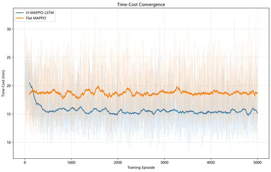
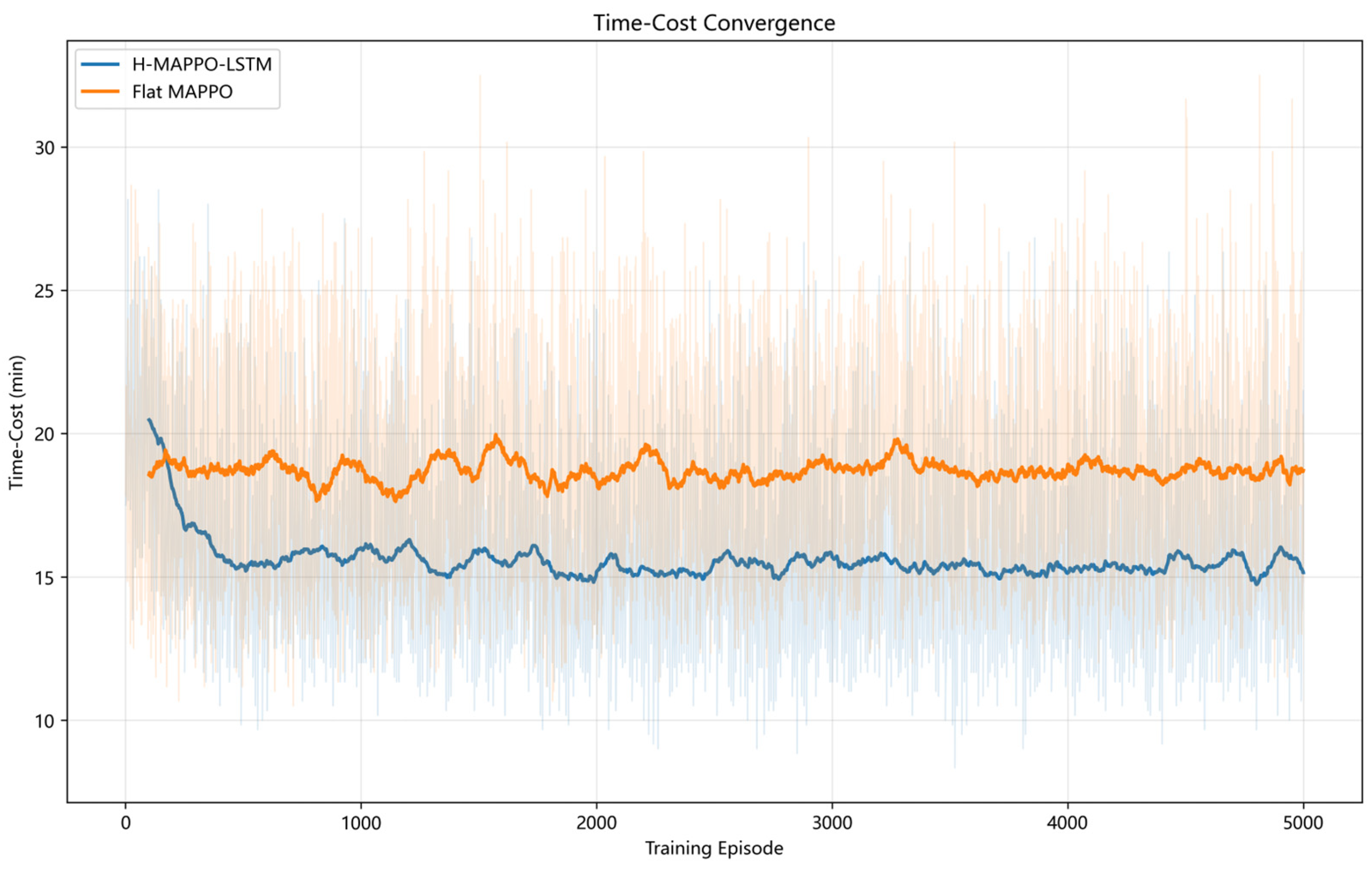
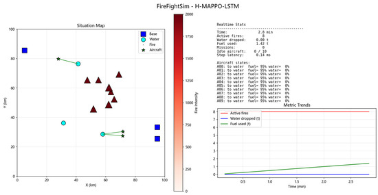
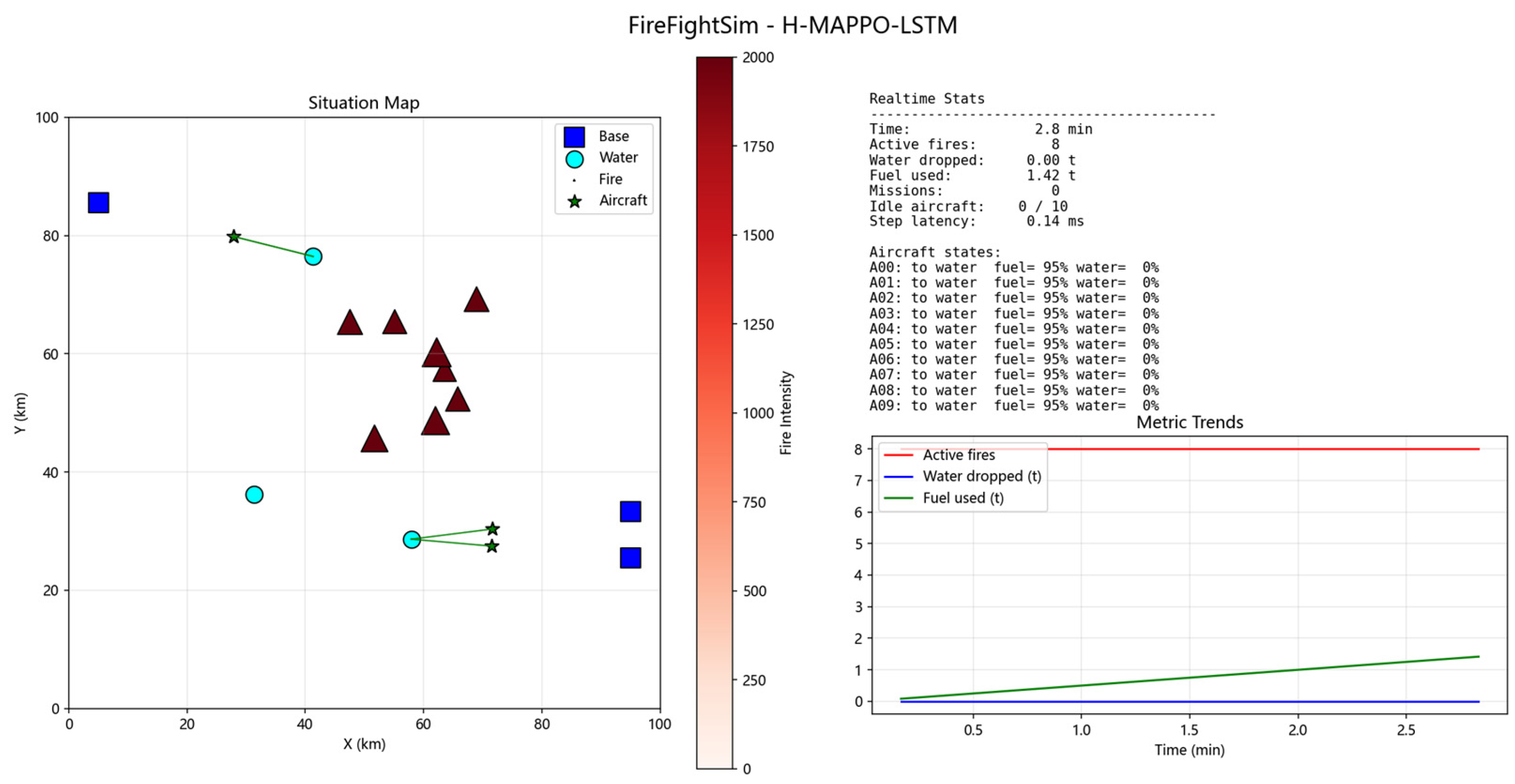
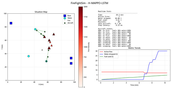
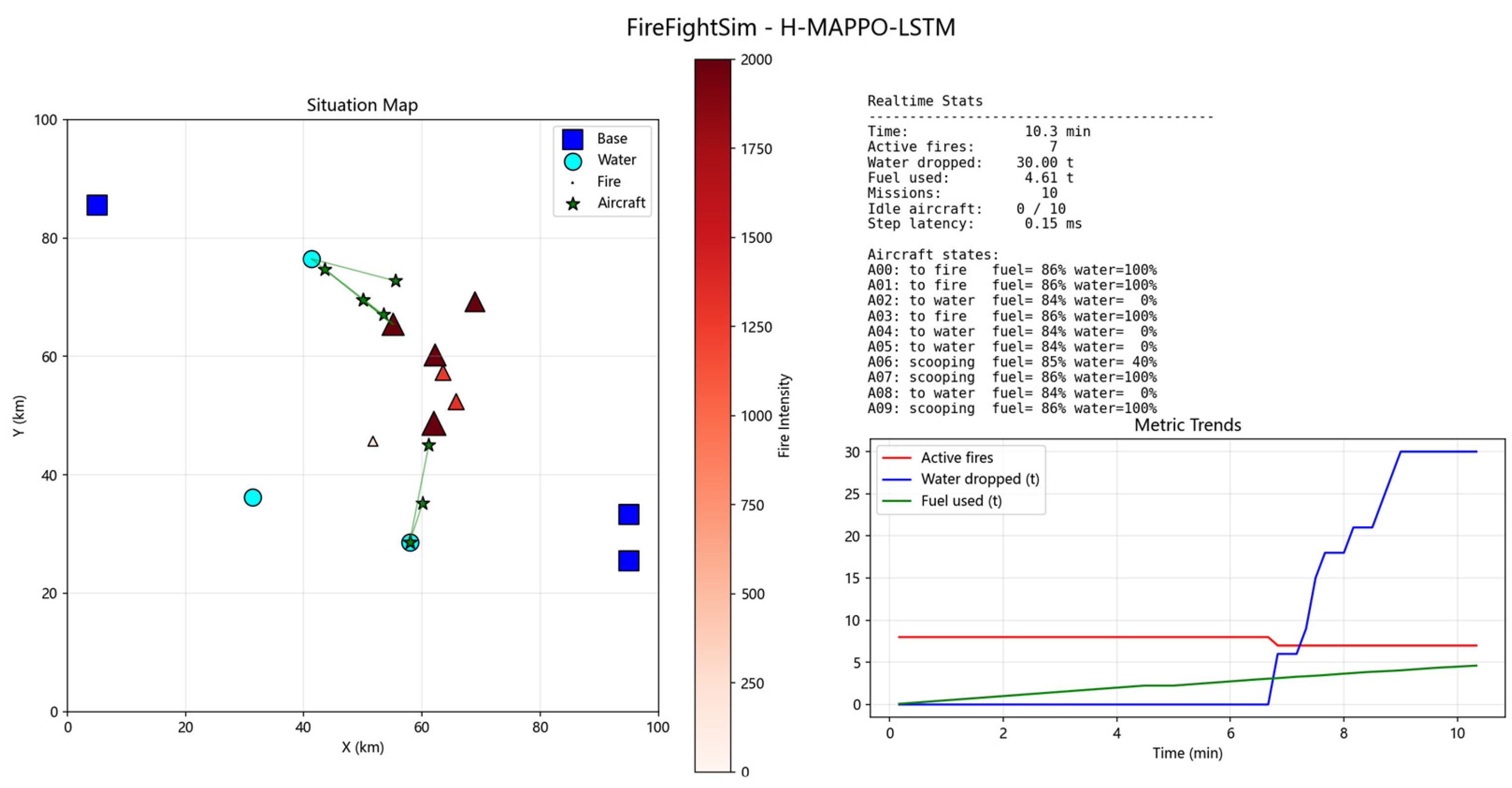
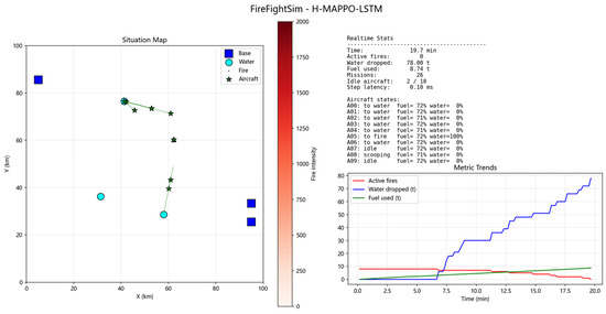
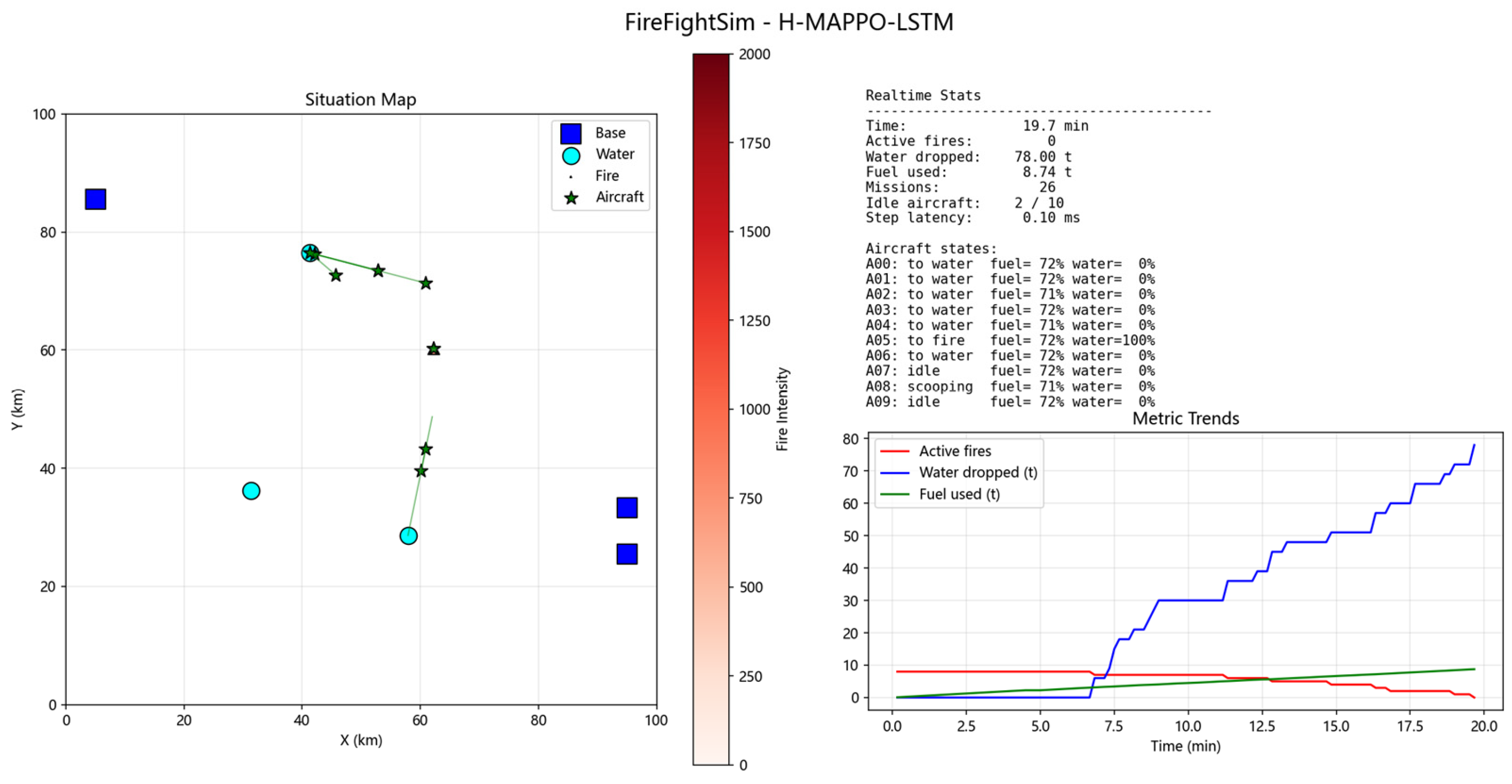
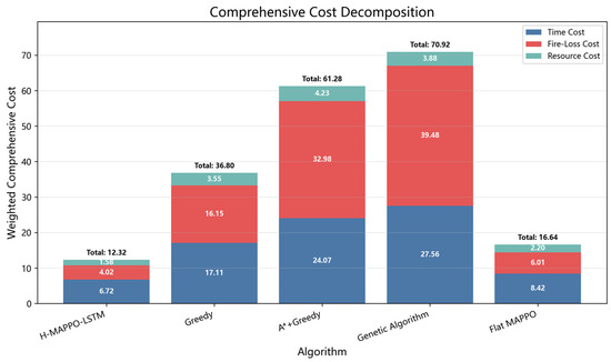
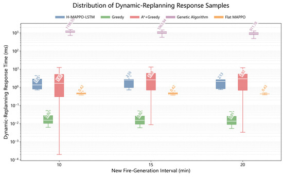
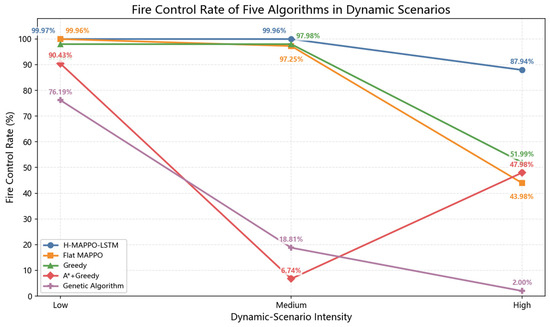
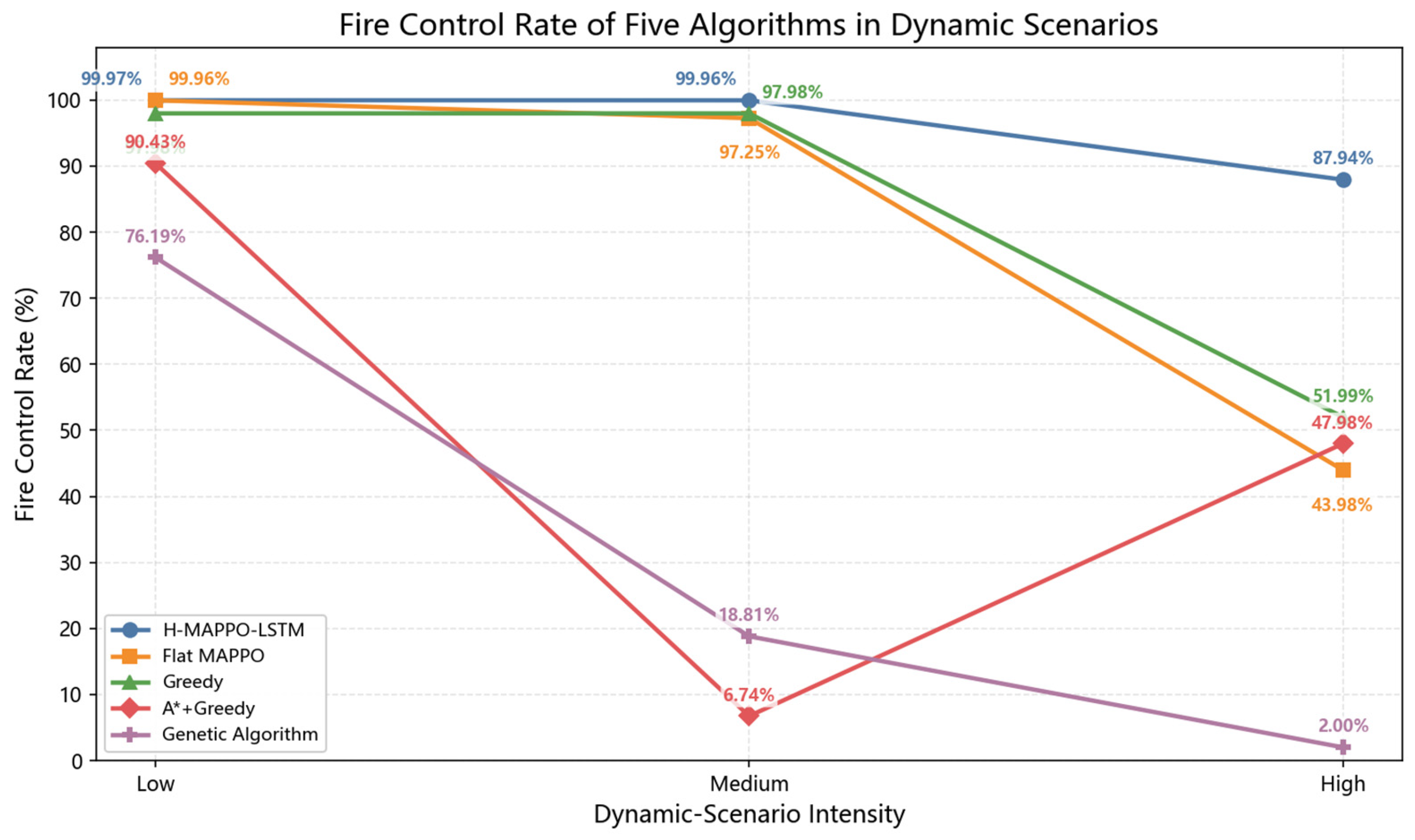
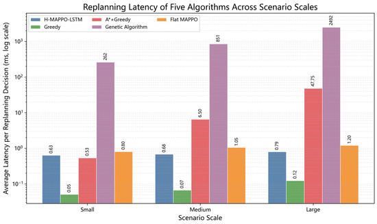
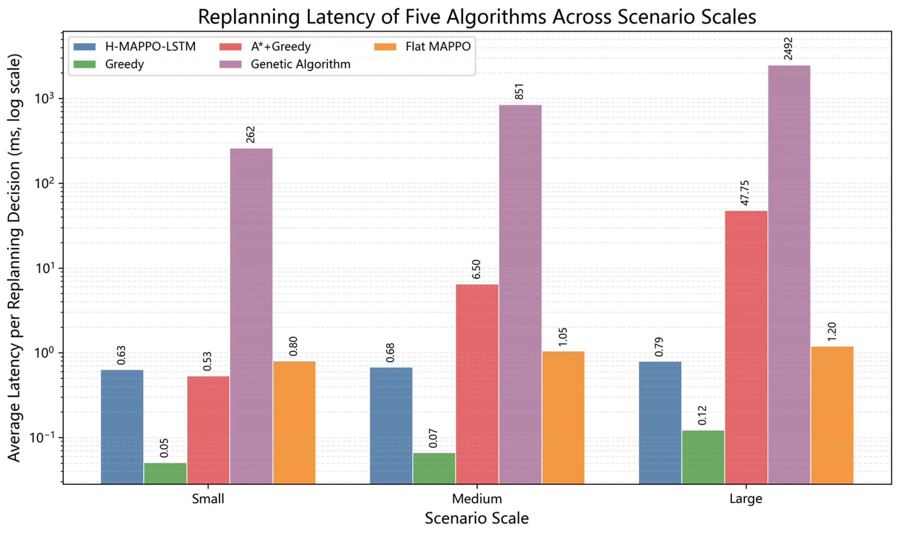
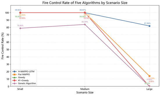
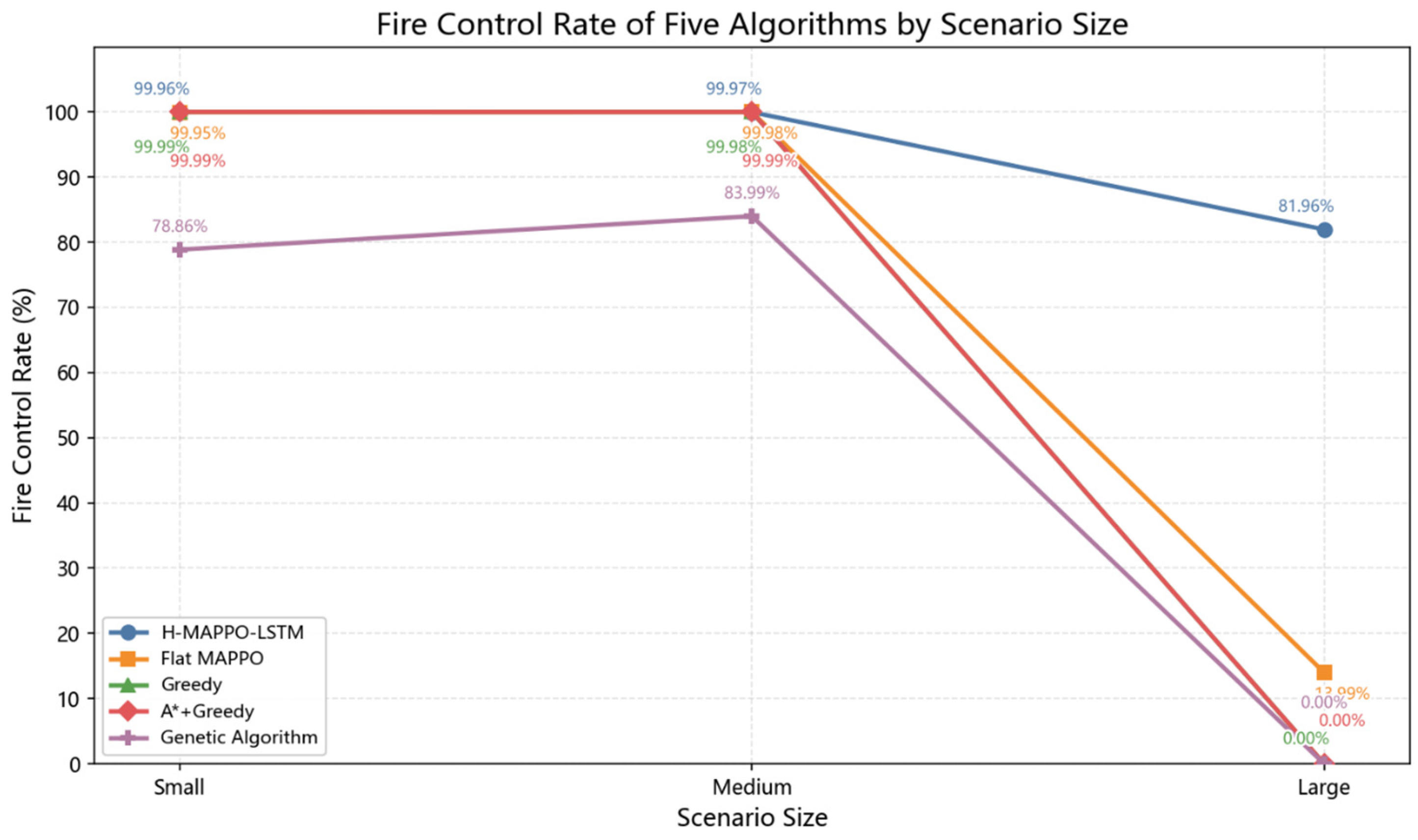
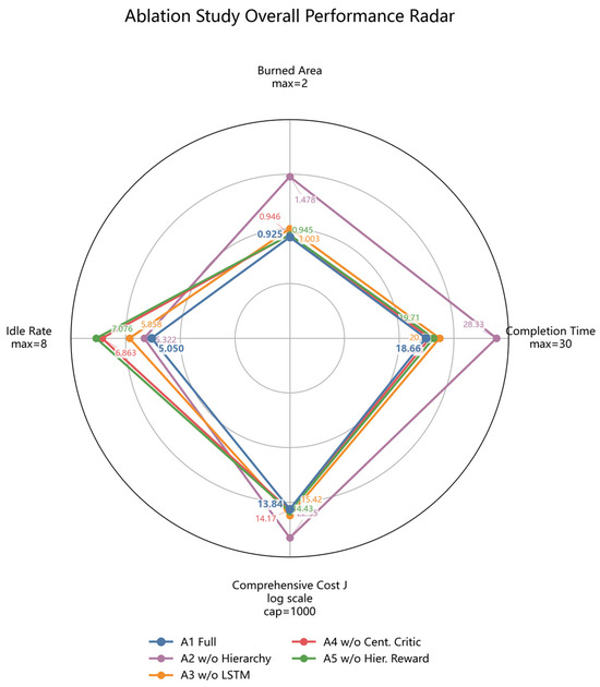
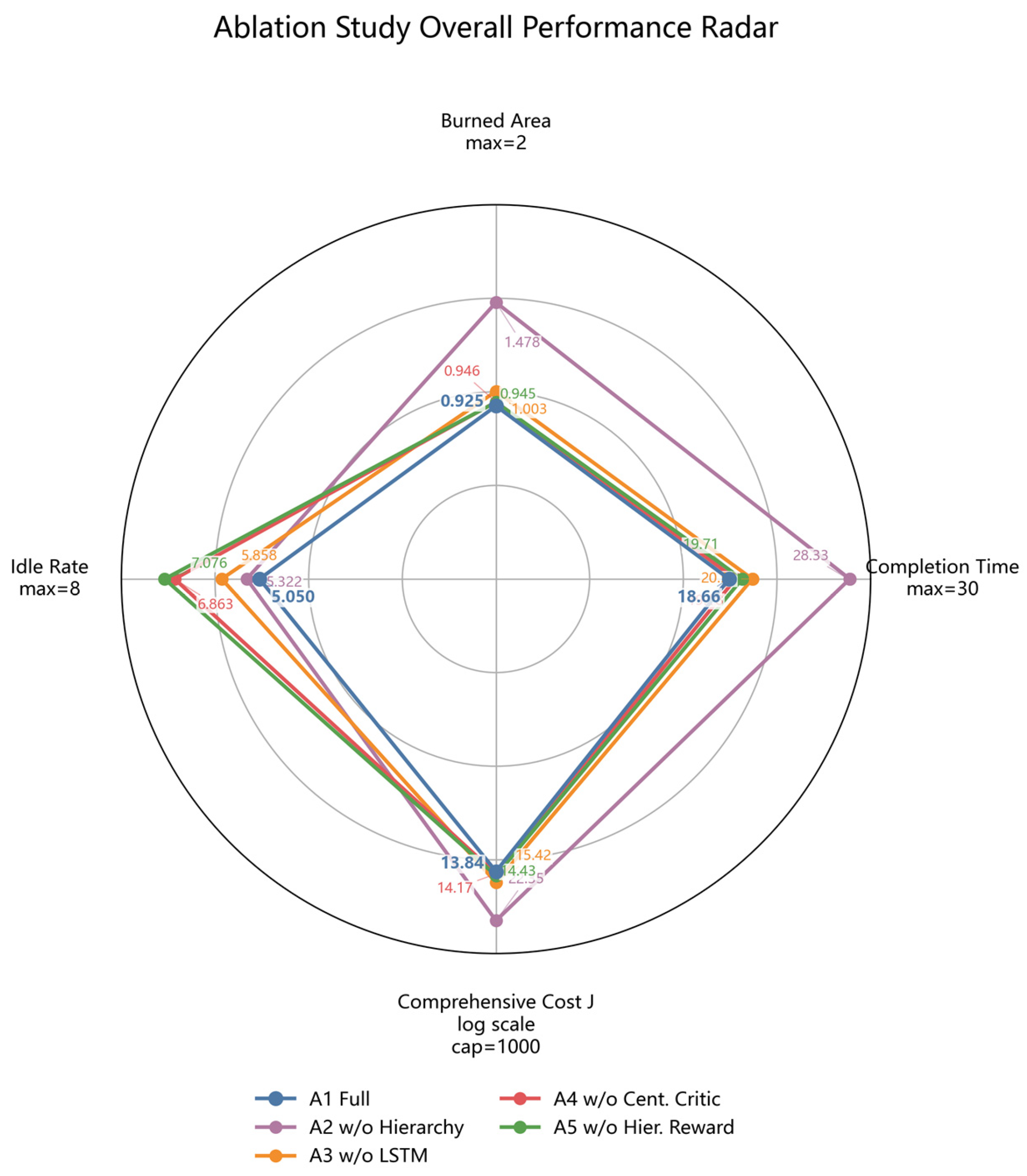
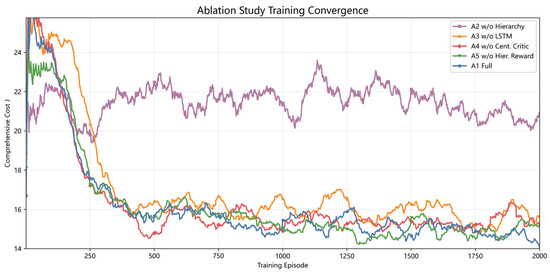
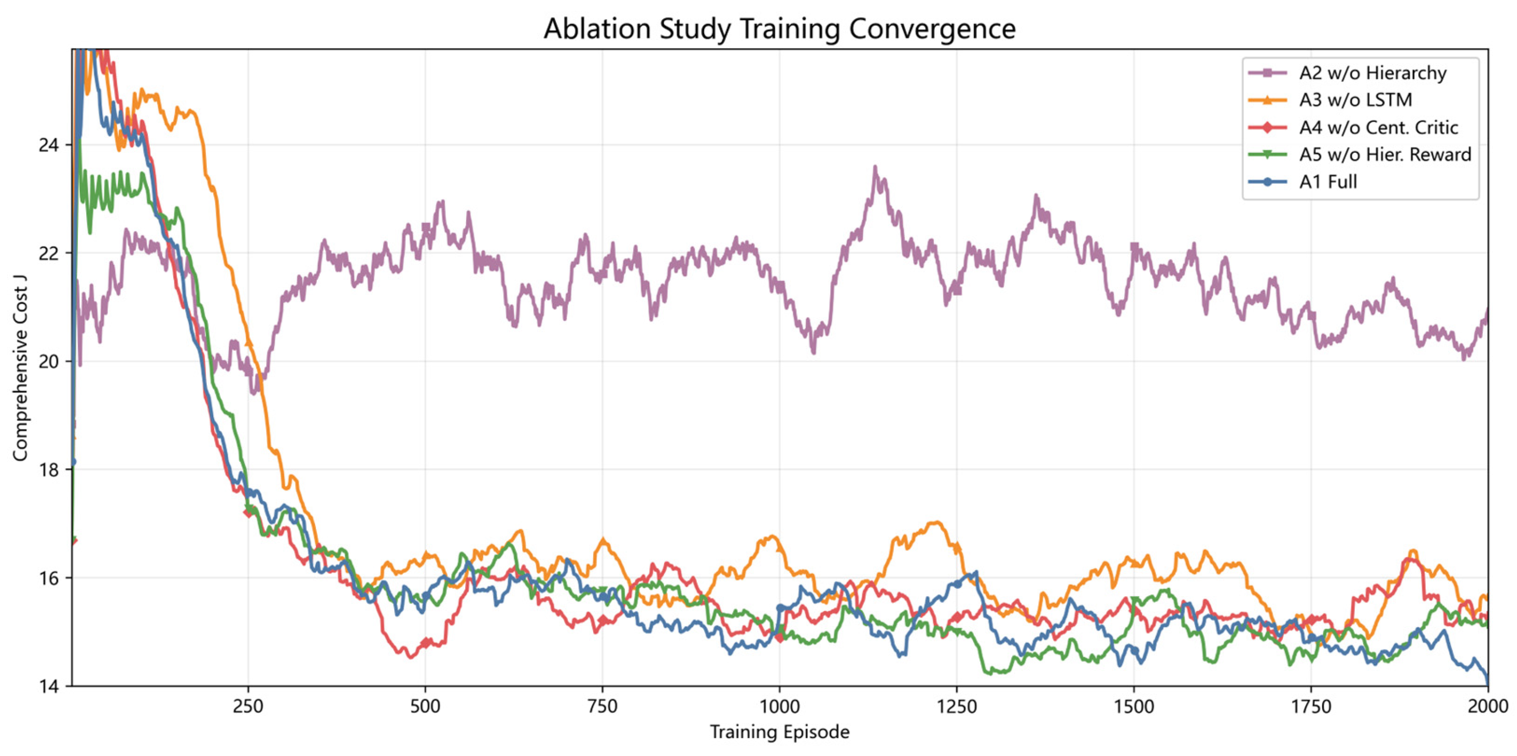

Disclaimer/Publisher’s Note: The statements, opinions and data contained in all publications are solely those of the individual author(s) and contributor(s) and not of MDPI and/or the editor(s). MDPI and/or the editor(s) disclaim responsibility for any injury to people or property resulting from any ideas, methods, instructions or products referred to in the content. |
© 2026 by the authors. Licensee MDPI, Basel, Switzerland. This article is an open access article distributed under the terms and conditions of the Creative Commons Attribution (CC BY) license.