Derivative-Free Kurchatov-Type Accelerating Iterative Method for Solving Nonlinear Systems: Dynamics and Applications

Abstract

Two novel Kurchatov-type first-order divided difference operators were designed, which were used for constructing the variable parameter of three derivative-free iterative methods. The convergence orders of the new derivative-free methods are 3, $(5+\sqrt{17})/2\approx 4.56$ and 5. The new derivative-free iterative methods with memory were applied to solve nonlinear ordinary differential equations (ODEs) and partial differential equations (PDEs) in numerical experiments. The dynamical behavior of our new methods with memory was studied by using dynamical plane. The dynamical planes showed that our methods had good stability.

1. Introduction

The main advantage of derivative-free methods is that a derivative-free method can be used for finding the solution of a non-differentiable nonlinear function $F(t)$. Compared to Newton’s method [1], derivative-free iterative methods do not require derivative in iterations. Numerous derivative-free iterative methods for finding the solution of nonlinear systems $F(t)=0$ have been proposed, where $F:D\subseteq {\mathrm{R}}^n\to {\mathrm{R}}^n$. Traub [2] proposed the well-known derivative-free iterative method

$$\left\{\begin{array}{c}{s}^{(k)}=t^{(k)}+VF(t^{(k)}),\\ t^{(k+1)}=t^{(k)}-{[s^{(k)},t^{(k)};F]}^{-1}F(t^{(k)}),\end{array}\right.$$

(1)

where $V\in R-\left\{0\right\}$. $[s^{(k)},t^{(k)};F]$ is the first-order divided difference operator, which is defined by [3]

$$\begin{array}{c}{[s^{(k)},t^{(k)};F]}_{ij}=\frac{(F_i(s_1^{(k)}\cdots ,s_{j-1}^{(k)},s_j^{(k)},t_{j+1}^{(k)},\cdots ,t_m^{(k)})-F_i(s_1^{(k)}\cdots ,s_{j-1}^{(k)},t_j^{(k)},t_{j+1}^{(k)},\cdots ,t_m^{(k)})}{(s_j^{(k)}-t_j^{(k)})},\\ 1\le i,j\le m.\end{array}$$

(2)

The error equation of the method in (1) is

$${\epsilon }^{(k+1)}=D_2(I+V{F}^{\prime }(\eta )){({\epsilon }^{(k)})}^2+O({({\epsilon }^{(k)})}^3),$$

(3)

where $\eta \in {\mathrm{R}}^n$ is the solution of $F(t)=0$, ${\epsilon }^{(k)}=t^{(k)}-\eta$ and $D_k=\frac{1}{k!}{F}^{\prime }{(\eta )}^{-1}{F}^{(k)}(\eta )\in L_k({\mathrm{R}}^n,{\mathrm{R}}^n),(k=2,3,\cdots )$. By adding one new iterative step to the method in (1), Chicharro et al. [4] designed the following iterative method with order three:

$$\left\{\begin{array}{c}{s}^{(k)}=t^{(k)}+VF(t^{(k)}),\\ z^{(k)}=t^{(k)}-{[s^{(k)},t^{(k)};F]}^{-1}F(t^{(k)}),\\ t^{(k+1)}=z^{(k)}-{[s^{(k)},z^{(k)};F]}^{-1}F(z^{(k)}),\end{array}\right.$$

(4)

satisfying the error equation

$${\epsilon }^{(k+1)}=D_2^2{(I+V{F}^{\prime }(\eta ))}^2{({\epsilon }^{(k)})}^3+O({({\epsilon }^{(k)})}^4).$$

(5)

Let us assume that $V=-F^{\prime }{(\eta )}^{-1}$ in (3) and (5); then, the order of the methods in (1) and (4) can be improved. Unfortunately, the solution $\eta \in {\mathrm{R}}^n$ is unknown. Generally, we handle this problem by replacing the constant parameter V with a variable parameter $V^{(k)}$. The method with variable parameter $V^{(k)}$ is called method with memory. The variable parameter $V^{(k)}$ is designed by using iterative sequences from the current and previous steps. Substituting the variable parameter $V^{(k)}=-{[s^{(k-1)},t^{(k-1)};F]}^{-1}$ for constant parameter V in the method in (1), Ahmad et al. [5] and Petković et al. [6] designed some efficient multi-step derivative-free iterative methods with memory. In order to design a new iterative method with memory, Kurchatov [7] obtained the following one-step method with memory:

$$t^{(k+1)}=t^{(k)}-{(A^{(k)})}^{-1}F(t^{(k)}),$$

(6)

where $A^{(k)}=[2t^{(k)}-t^{(k-1)},t^{(k-1)};F]$ is called Kurchatov’s divided difference operator. Argyros et al. [8,9] studied the convergence properties of Kurchatov’s method (6) in the Banach space and proved that Kurchatov’s method is second-order convergent. Wang et al. [10] and Cordero et al. [11] presented some Kurchatov-type methods with memory by using Kurchatov’s divided difference operator.

Replacing V in (3) with $V^{(k)}=-{(A^{(k)})}^{-1}$, Chicharro et al. [4] obtained the following method with memory:

$$\left\{\begin{array}{c}{s}^{(k)}=t^{(k)}+V^{(k)}F(t^{(k)}),\\ t^{(k+1)}=t^{(k)}-{[s^{(k)},t^{(k)};F]}^{-1}F(t^{(k)}),\end{array}\right.$$

(7)

where $V^{(k)}=-{[2t^{(k)}-t^{(k-1)},t^{(k-1)};F]}^{-1}.$ The method in (7) is called FM3 in Chicharro’s paper [4]. Substituting $V^{(k)}=-{(A^{(k)})}^{-1}$ for the parameter V in (4), they obtained the following scheme with memory:

$$\left\{\begin{array}{c}{s}^{(k)}=t^{(k)}+V^{(k)}F(t^{(k)}),\\ z^{(k)}=t^{(k)}-{[s^{(k)},t^{(k)};F]}^{-1}F(t^{(k)}),\\ t^{(k+1)}=z^{(k)}-{[s^{(k)},z^{(k)};F]}^{-1}F(z^{(k)}).\end{array}\right.$$

(8)

The method in (8) is called FM5 in Chicharro’s paper [4]. They concluded that the convergence orders of the FM3 and FM5 methods were 3 and 5, respectively. However, their conclusions about convergence order were incorrect and the results of numerical experiment were inconsistent with their theoretical results. The main reason of this mistake is that they wrongly used the following equation in the paper [4]:

$$I+V^{(k)}{F}^{\prime }(\eta )=D_3{({\epsilon }^{(k-1)})}^2+2D_2{\epsilon }^{(k)}-2D_3{\epsilon }^{(k-1)}{\epsilon }^{(k)}+O({\epsilon }^{(k-1)},{\epsilon }^{(k)}),$$

(9)

where

$$V^{(k)}\sim -[I-D_3{({\epsilon }^{(k-1)})}^2+2D_3{\epsilon }^{(k-1)}{\epsilon }^{(k)}-2D_2{\epsilon }^{(k)}]F^{\prime }{(\eta )}^{-1}.$$

(10)

For the iterative FM3 and FM5 methods, the error ${\epsilon }^{(k)}$ is less than the error ${({\epsilon }^{(k-1)})}^2$. So, Equation (9) should be written as

$$I+V^{(k)}{F}^{\prime }(\eta )\sim D_3{({\epsilon }^{(k-1)})}^2.$$

(11)

Theorem 1.

Let the nonlinear function $F:D\subset {\mathrm{R}}^n\to {\mathrm{R}}^n$ be sufficiently differentiable and $\eta \in {\mathrm{R}}^n$ be a zero of F. Let us assume that the initial value $t^{(0)}$ is close to η. Then, the FM3 and FM5 methods have convergence orders $1+\sqrt{3}\approx 2.732$ and 4, respectively.

Proof. 

Let r and p be the convergence orders of the FM3 and FM5 methods, respectively. The error relation of FM3 can be written as

$${\epsilon }^{(k+1)}\sim A_{k,r}{({\epsilon }^{(k)})}^r,$$

(12)

where $A_{k,r}$ is the asymptotic error constant. So,

$${\epsilon }^{(k+1)}\sim A_{k,r}{(A_{k-1,r}{({\epsilon }^{(k-1)})}^r)}^r=A_{k,r}{A}_{k-1,r}^r{({\epsilon }^{(k-1)})}^{r^2}.$$

(13)

By replacing $I+V{F}^{\prime }(\eta )$ of (3) with (11), we obtain the error expression of the FM3 method.

$${\epsilon }^{(k+1)}\sim D_2{D}_3{A}_{k-1,r}^2{({\epsilon }^{(k-1)})}^{2r+2}.$$

(14)

The asymptotic error constants $A_{k,r}{A}_{k-1,r}^r$ in (13) and $D_2{D}_3{A}_{k-1,r}^2$ in (14) do not affect the convergence order of the iterative method. By equating the appropriate exponents of ${\epsilon }^{(k-1)}$ in (13) and (14), we have

$$r^2-2r-2=0.$$

(15)

By solving Equation (15), we obtain the positive root $r=1+\sqrt{3}\approx 2.732.$ This implies that the order of the FM3 method is $2.732.$

Similar to Equations (12) and (13), the error relation of the FM5 method can be given by

$${\epsilon }^{(k+1)}\sim A_{k,p}{({\epsilon }^{(k)})}^p,$$

(16)

and

$${\epsilon }^{(k+1)}\sim A_{k,p}{A}_{k-1,p}^p{({\epsilon }^{(k-1)})}^{p^2}.$$

(17)

By replacing $I+V{F}^{\prime }(\eta )$ of (5) with (11), we obtain the error relation

$${\epsilon }^{(k+1)}\sim D_2^2{D}_3^2{A}_{k-1,p}^2{({\epsilon }^{(k-1)})}^{3p+4}.$$

(18)

From (17) and (18), we obtain

$$p^2-3p-4=0.$$

(19)

By solving Equation (19), we obtain $p=4$ and $p=-1$. The convergence order of iterative method should be positive, so $p=-1$ is discarded. This implies that the convergence order of the FM5 method is four. □

Theorem 1 obtains the true order of the FM3 and FM5 methods.

Remark 1.

From the error Equation (5) of the iterative method in (4) without memory, we know that ${\epsilon }^{(k+1)}\sim {({\epsilon }^{(k)})}^3$ and ${\epsilon }^{(k)}\sim {({\epsilon }^{(k-1)})}^3$. Thus, the error ${\epsilon }^{(k)}$ is less than the error ${({\epsilon }^{(k-1)})}^2$. The FM5 method with memory improves the convergence order of the method in (4) by the variable parameter $V^{(k)}$. By replacing $I+V{F}^{\prime }(\eta )$ of (5) with (9), we obtain ${\epsilon }^{(k+1)}=D_2^2{(D_3{({\epsilon }^{(k-1)})}^2+2D_2{\epsilon }^{(k)}-2D_3{\epsilon }^{(k-1)}{\epsilon }^{(k)})}^2{({\epsilon }^{(k)})}^3+O({({\epsilon }^{(k)})}^4).$ This means that the error ${\epsilon }^{(k+1)}$ of the FM5 method is less than ${({\epsilon }^{(k)})}^3$ and ${\epsilon }^{(k)}$ of FM5 method is less than ${({\epsilon }^{(k-1)})}^2$. For the FM3 method with memory, we also obtain that ${\epsilon }^{(k+1)}=D_2(D_3{({\epsilon }^{(k-1)})}^2+2D_2{\epsilon }^{(k)}-2D_3{\epsilon }^{(k-1)}{\epsilon }^{(k)}){({\epsilon }^{(k)})}^2+O({({\epsilon }^{(k)})}^3).$ This means that the error ${\epsilon }^{(k)}$ of the FM3 method is less than ${({\epsilon }^{(k-1)})}^2$. Thus, we obtain the error Equation (11).

Inspired by the FM3 and FM5 methods, we propose three iterative methods with a novel variable parameter in the next section.

The structure of this paper is as follows: The design of two novel divided difference operators as the variable parameters of three derivative-free iterative methods with memory for solving nonlinear systems is presented in Section 2. Using the new Kurchatov-type divided difference, the new derivative-free iterative methods reached the orders 3, $(5+\sqrt{17})/2\approx 4.56$ and 5, respectively. In Section 3, the application of the proposed methods to solve the ODEs, PDEs, the standard nonlinear systems and the non-differentiable nonlinear systems is presented. In Section 4, the dynamical behavior of the presented method is studied for analyzing the stability of the presented methods. In Section 5, we give a short summary.

2. Two New Kurchatov-Type Accelerating Derivative-Free Iterative Methods with Memory

In this section, two new first-order divided difference operators are used for constructing the variable parameter $V^{(k)}$. Similar to Kurchatov’s first-order divided difference, we construct the following first-order divided differences

$$[2t^{(k)}-s^{(k-1)},s^{(k-1)};F]$$

(20)

and

$$[2t^{(k)}-z^{(k-1)},z^{(k-1)};F].$$

(21)

We call (20) and (21) Kurchatov-type first-order divided differences.

Method 1: Using (20), we obtain $V^{(k)}=-{[2t^{(k)}-s^{(k-1)},s^{(k-1)};F]}^{-1}$.

By replacing ${\epsilon }^{(k-1)}$ with ${\epsilon }_s^{(k-1)}$ in Equations (10) and (11), we obtain

$$V^{(k)}\sim -[I-D_3{({\epsilon }_s^{(k-1)})}^2-2D_2{\epsilon }^{(k)}+2D_3{\epsilon }_s^{(k-1)}{\epsilon }^{(k)}]F^{\prime }{(\eta )}^{-1},$$

(22)

where ${\epsilon }_s^{(k-1)}=s^{(k-1)}-\eta$.

Method 2: Using (21), we obtain $V^{(k)}=-{[2t^{(k)}-z^{(k-1)},z^{(k-1)};F]}^{-1}$.

By replacing ${\epsilon }^{(k-1)}$ with ${\epsilon }_z^{(k-1)}$ in Equations (10) and (11), we obtain

$$V^{(k)}\sim -[I-D_3{({\epsilon }_z^{(k-1)})}^2-2D_2{\epsilon }^{(k)}+2D_3({\epsilon }_z^{(k-1)}){\epsilon }^{(k)}]F^{\prime }{(\eta )}^{-1},$$

(23)

where ${\epsilon }_z^{(k-1)}=z^{(k-1)}-\eta$.

By substituting (22) for $V^{(k)}$ of the FM3 method, we obtain the following scheme with memory:

$$\left\{\begin{array}{c}{s}^{(k)}=t^{(k)}-{[2t^{(k)}-s^{(k-1)},s^{(k-1)};F]}^{-1}F(t^{(k)}),\\ t^{(k+1)}=t^{(k)}-{[s^{(k)},t^{(k)};F]}^{-1}F(t^{(k)}).\end{array}\right.$$

(24)

The convergence order of the proposed scheme (24) is given by the following theorem.

Theorem 2.

Let $F:D\subset {\mathrm{R}}^n\to {\mathrm{R}}^n$ be a sufficiently differentiable function in an open neighborhood D and $\eta \in {\mathrm{R}}^n$ be a zero of function F. Let us assume that the initial value $t^{(0)}$ is close enough to η. Then, the convergence order of the iterative scheme in (24) is three.

Proof. 

From (22) and (24), we have

$${\epsilon }_s^{(k)}=s^{(k)}-\eta =t^{(k)}-\eta -{[2t^{(k)}-s^{(k-1)},s^{(k-1)};F]}^{-1}F(t^{(k)})$$

$$=(D_3{({\epsilon }_s^{(k-1)})}^2+2D_2{\epsilon }^{(k)}-2D_3{\epsilon }_s^{(k-1)}{\epsilon }^{(k)}){\epsilon }^{(k)}.$$

(25)

and

$${({\epsilon }_s^{(k)})}^2={(D_3{({\epsilon }_s^{(k-1)})}^2+2D_2{\epsilon }^{(k)}-2D_3{\epsilon }_s^{(k-1)}{\epsilon }^{(k)})}^2{({\epsilon }^{(k)})}^2.$$

(26)

By replacing V of (3) with (22),

$${\epsilon }^{(k+1)}=D_2(I+V^{(k)}{F}^{\prime }(\eta )){({\epsilon }^{(k)})}^2+O({({\epsilon }^{(k)})}^3)$$

$$=D_2(D_3{({\epsilon }_s^{(k-1)})}^2+2D_2{\epsilon }^{(k)}-2D_3{\epsilon }_s^{(k-1)}{\epsilon }^{(k)}){({\epsilon }^{(k)})}^2+O({({\epsilon }^{(k)})}^3),$$

(27)

By comparing (26) with (27), we know that ${({\epsilon }_s^{(k)})}^2$ is less than ${\epsilon }^{(k+1)}$ and ${({\epsilon }_s^{(k-1)})}^2$ is less than ${\epsilon }^{(k)}$. From (22), we obtain

$$I+V^{(k)}{F}^{\prime }(\eta )\sim D_3{({\epsilon }_s^{(k-1)})}^2+2D_2{\epsilon }^{(k)}-2D_3{\epsilon }_s^{(k-1)}{\epsilon }^{(k)}$$

$$\sim 2D_2({\epsilon }^{(k)}),$$

(28)

From (27) and (28), we obtain

$${\epsilon }^{(k+1)}\sim 2D_2^2{({\epsilon }^{(k)})}^3,$$

(29)

This implies that the method in (24) has order three. □

Remark 2.

We note that the method in (24) and the FM3 method have the same computational costs with different convergence orders. Our method (24) has a higher convergence order than the FM3 method. So, the computational efficiency of the FM3 method is less than that of the method in (24).

By replacing $V^{(k)}$ of the FM5 method with (22), we obtain the following scheme with memory:

$$\left\{\begin{array}{c}{s}^{(k)}=t^{(k)}-{[2t^{(k)}-s^{(k-1)},s^{(k-1)};F]}^{-1}F(t^{(k)}),\\ z^{(k)}=t^{(k)}-{[s^{(k)},t^{(k)};F]}^{-1}F(t^{(k)}),\\ t^{(k+1)}=z^{(k)}-{[s^{(k)},z^{(k)};F]}^{-1}F(z^{(k)}).\end{array}\right.$$

(30)

By replacing $V^{(k)}$ of the FM5 method with (23), we obtain

$$\left\{\begin{array}{c}{s}^{(k)}=t^{(k)}-{[2t^{(k)}-z^{(k-1)},z^{(k-1)};F]}^{-1}F(t^{(k)}),\\ z^{(k)}=t^{(k)}-{[s^{(k)},t^{(k)};F]}^{-1}F(t^{(k)}),\\ t^{(k+1)}=z^{(k)}-{[s^{(k)},z^{(k)};F]}^{-1}F(z^{(k)}).\end{array}\right.$$

(31)

The convergence orders of the proposed schemes in (30) and (31) are given by the following result.

Theorem 3.

Let $F:D\subset {\mathrm{R}}^n\to {\mathrm{R}}^n$ be a sufficiently differentiable function in an open neighborhood D and $\eta \in {\mathrm{R}}^n$ be a zero of function F. Let us assume that the initial value $t^{(0)}$ is close enough to η. Then, the iterative methods in (30) and (31) have convergence orders $(5+\sqrt{17})/2\approx 4.56$ and 5, respectively.

Proof. 

Let $H^{(k)}=I+V^{(k)}{F}^{\prime }(\eta )$. Using (22), we have

$$H^{(k)}=D_3{({\epsilon }_s^{(k-1)})}^2+2D_2{\epsilon }^{(k)}-2D_3{\epsilon }_s^{(k-1)}{\epsilon }^{(k)}.$$

(32)

Using (5), (30) and (32), we obtain

$${\epsilon }^{(k+1)}\sim D_2^2{(I+V^{(k)}{F}^{\prime }(\eta ))}^2{({\epsilon }^{(k)})}^3$$

$$\sim D_2^2{(H^{(k)})}^2{({\epsilon }^{(k)})}^3$$

$$\sim D_2^2{(D_3{({\epsilon }_s^{(k-1)})}^2+2D_2{\epsilon }^{(k)}-2D_3{\epsilon }_s^{(k-1)}{\epsilon }^{(k)})}^2{({\epsilon }^{(k)})}^3.$$

(33)

By comparing (26) with (33), we know that ${({\epsilon }_s^{(k)})}^2$ is more than ${\epsilon }^{(k+1)}$ and ${({\epsilon }_s^{(k-1)})}^2$ is more than ${\epsilon }^{(k)}$. From (32), we obtain

$$H^{(k)}\sim D_3{({\epsilon }_s^{(k-1)})}^2$$

$$\sim D_3{(I+V^{(k-1)}{F}^{\prime }(\eta ))}^2{({\epsilon }^{(k-1)})}^2$$

$$\sim D_3^3{(H^{(k-2)})}^4{({\epsilon }^{(k-2)})}^4{({\epsilon }^{(k-1)})}^2$$

$$\sim D_3^{2^{k-1}}{(H^{(0)})}^{2^j}{({\epsilon }^{(0)})}^{2^k}{({\epsilon }^{(1)})}^{2^{k-1}}{({\epsilon }^{(2)})}^{2^{k-2}}\cdots {({\epsilon }^{(k-2)})}^{2^2}{({\epsilon }^{(k-1)})}^2.$$

(34)

where ${\epsilon }^{(k)}=t^{(k)}-\eta ,(k=0,1,\cdots ,n).$ Let us assume that the sequence $\left\{t^{(k)}\right\}$ generated by the iterative method satisfies

$${\epsilon }^{(k+1)}\sim A_{k+1}{({\epsilon }^{(0)})}^{r_{k+1}},0\le k\le n,$$

(35)

where ${\epsilon }^{(k+1)}=t^{(k+1)}-\eta$ and $A_{k+1}$ is an asymptotic error constant.

From (33) and (34), we have

$${\epsilon }^{(k+1)}\sim D_2^2{(H^{(k)})}^2{({\epsilon }^{(k)})}^3$$

$$\sim D_2^2{D}_3^{2^k}{(H(0))}^{2^{k+1}}{({\epsilon }^{(0)})}^{2^{k+1}}{(A_1{({\epsilon }^{(0)})}^{r_1})}^{2^k}{(A_2{({\epsilon }^{(0)})}^{r_2})}^{2^{k-1}}\cdots$$

$$\times {(A_{k-2}{({\epsilon }^{(0)})}^{r_{k-2}})}^{2^3}{(A_{k-1}{({\epsilon }^{(0)})}^{r_{k-1}})}^{2^2}{(A_k{({\epsilon }^{(0)})}^{r_k})}^3.$$

(36)

From (35) and (36), we obtain

$$r_{k+1}=2^{k+1}+2^k{r}_1+2^{k-1}{r}_2+\cdots +2^3{r}_{k-2}+2^2{r}_{k-1}+3r_k,$$

(37)

and

$$r_k=2^k+2^{k-1}{r}_1+2^{k-2}{r}_2+\cdots +2^2{r}_{k-2}+3r_{k-1}.$$

(38)

From (37) and (38), we have

$$r_{k+1}-2r_k=-2r_{k-1}+3r_k,$$

(39)

and

$$\frac{r_{k+1}}{r_k}=5-\frac{2r_{k-1}}{r_k}.$$

(40)

By letting $\underset{k\to \infty }{lim}(r_{k+1}/r_k)=\underset{k\to \infty }{lim}(r_k/r_{k-1})=Or$, we obtain

$$Or=5-2\frac{1}{Or},$$

(41)

where $Or$ is a constant. By solving Equation (41), we obtain $Or=\left(5+\sqrt{17}\right)/2$. This implies that the convergence order of the method in (30) is $Or=\left(5+\sqrt{17}\right)/2\approx 4.56$.

From (5) and (23), we obtain

$$I+V^{(k)}{F}^{\prime }(\eta )\sim 2D_2{\epsilon }^{(k)},$$

(42)

and

$${\epsilon }^{(k+1)}\sim D_2^2{(I+V^{(k)}{F}^{\prime }(\eta ))}^2{({\epsilon }^{(k)})}^3\sim 4D_2^4{({\epsilon }^{(k)})}^5.$$

(43)

This implies that the order of the method with memory in (31) is five. □

Remark 3.

Theorem 3 shows that the convergence order of the method in (4) without memory is improved from three to five by using one accelerating parameter (23). The convergence orders of the methods in (30) and (31) are higher than that of the FM5 method. The computational efficiency index (CEI) [3] is defined by $CEI={\rho }^{\frac{1}{c}}$, where ρ is the convergence order and c is the computational cost of the iterative method. The methods in (30) and (31) and the FM5 method have different convergence orders with the same computational costs. We know that the computational efficiency of our methods shown in (30) and (31) is superior to that of the FM5 method.

Remark 4.

The methods in (24) and (30) use the same accelerating parameter (22). In Theorems 2 and 3, we use the different error relations of the parameter (22). The main reason is that (${\epsilon }_s^{(k-1)}{)}^2$ in (22) is less than ${\epsilon }^{(k)}$ for the two-step method method in (24) and ${({\epsilon }_s^{(k-1)})}^2$ in (22) is more than ${\epsilon }^{(k)}$ for the three-step method in (30).

Remark 5.

In order to simplify calculation, the computational scheme of the method in (30) can be written as

$$\left\{\begin{array}{c}[2t^{(k)}-s^{(k-1)},s^{(k-1)};F]{\beta }_1^{(k)}=F(t^{(k)}),s^{(k)}=t^{(k)}-{\beta }_1^{(k)},\\ [s^{(k)},t^{(k)};F]{\beta }_2^{(k)}=F(t^{(k)}),z^{(k)}=t^{(k)}-{\beta }_2^{(k)},\\ [s^{(k)},z^{(k)};F]{\beta }_3^{(k)}=F(z^{(k)}),t^{(k+1)}=z^{(k)}-{\beta }_3^{(k)}.\end{array}\right.$$

(44)

The computational scheme of the method in (31) can be written as

$$\left\{\begin{array}{c}[2t^{(k)}-z^{(k-1)},z^{(k-1)};F]{\gamma }_1^{(k)}=F(t^{(k)}),s^{(k)}=t^{(k)}-{\gamma }_1^{(k)},\\ [s^{(k)},t^{(k)};F]{\gamma }_2^{(k)}=F(t^{(k)}),z^{(k)}=t^{(k)}-{\gamma }_2^{(k)},\\ [s^{(k)},z^{(k)};F]{\gamma }_3^{(k)}=F(z^{(k)}),t^{(k+1)}=z^{(k)}-{\gamma }_3^{(k)}.\end{array}\right.$$

(45)

The linear systems in (37) and (38) were solved by LU decomposition in numerical experiments.

3. Numerical Results

The methods in (24), (30) and (31) were compared with Chicharro’s methods (4), FM3 and FM5, for solving ODEs, PDEs and standard nonlinear systems. All the experiments were carried by the Maple 14 computer algebra system (Digits: = 2048). The parameter $V^{(0)}$ was the identity matrix. The solution was obtained by the stopping criterion $\left|\right|t^{(k)}-t^{(k-1)}\left|\right|<{10}^{-100}$.

Table 1, Table 2, Table 3, Table 4, Table 5 and Table 6 show the following information: ACOC [12] is the approximated computational order of convergence, NIT (number of iterations) is the number of iterations, EVL is evaluation of error $\left|\right|t^{(k)}-t^{(k-1)}\left|\right|$ at the last step, T is the CPU time and FU is function values at the last step. 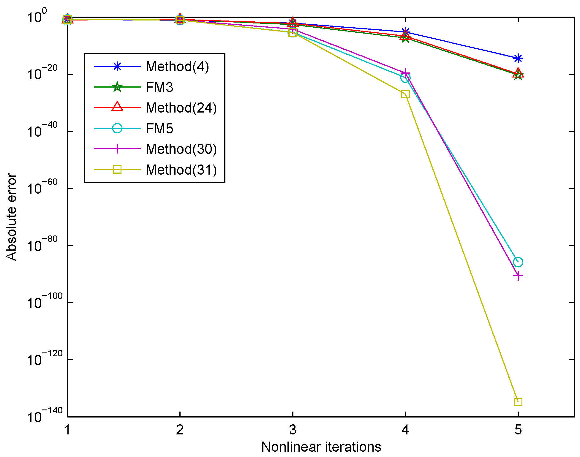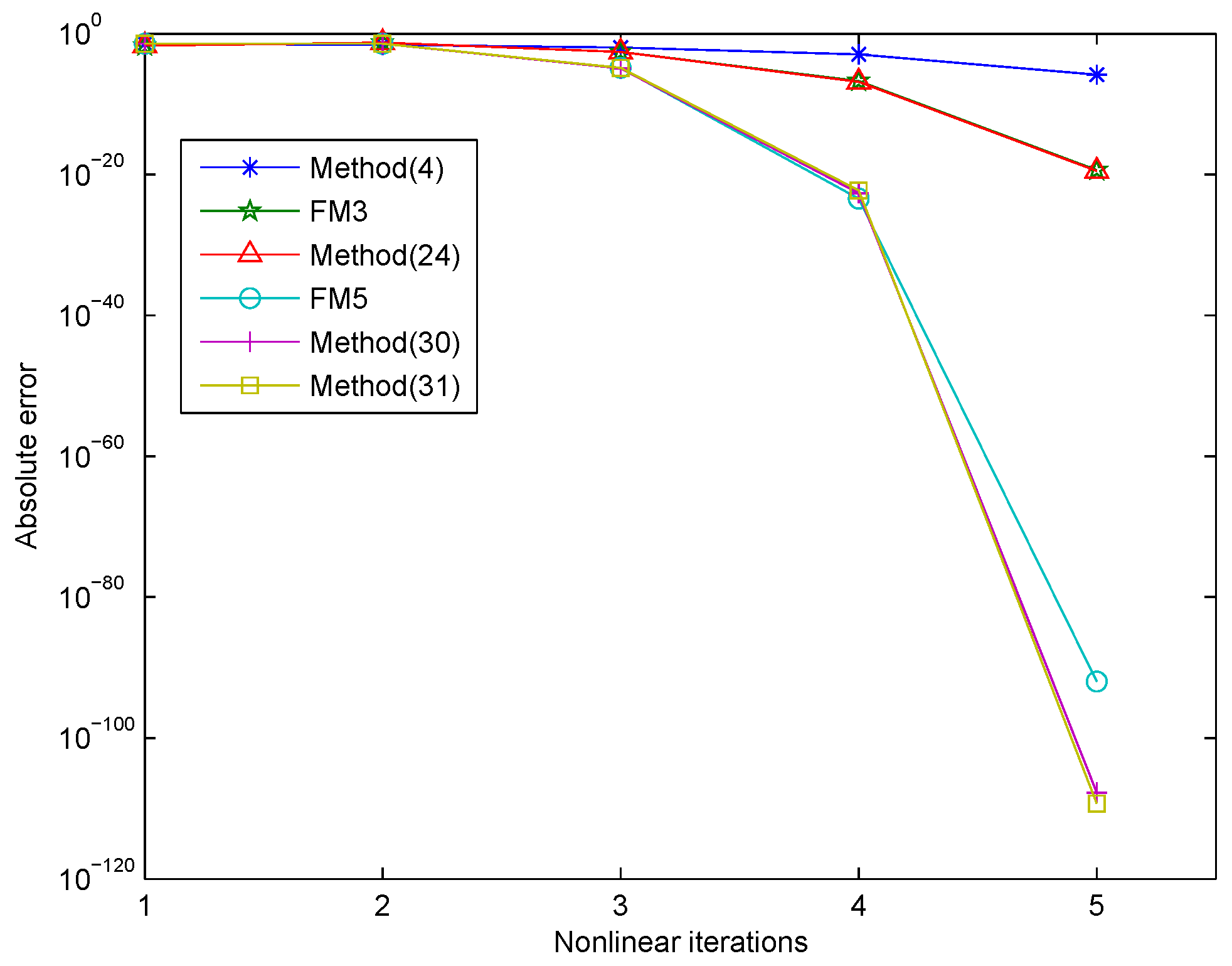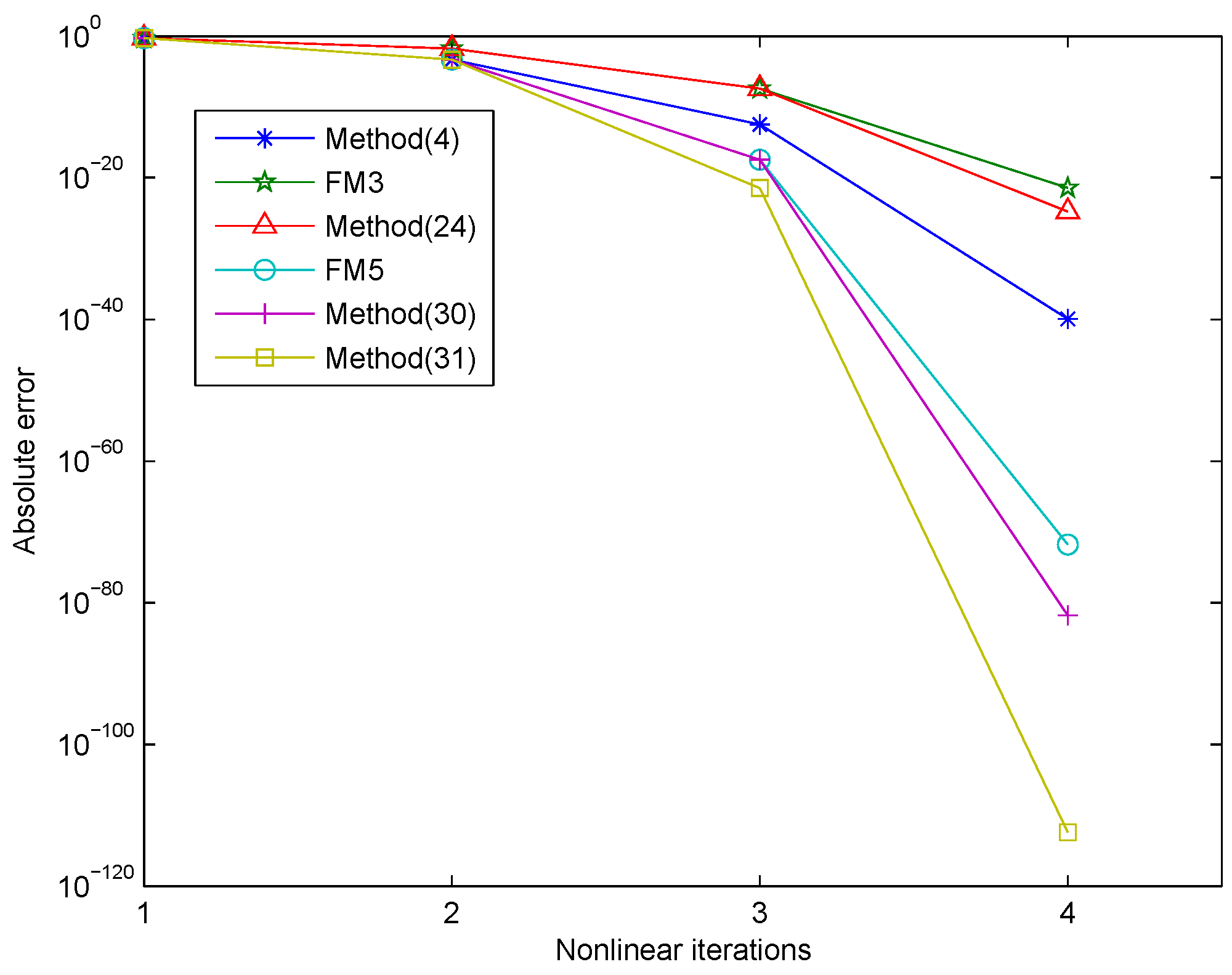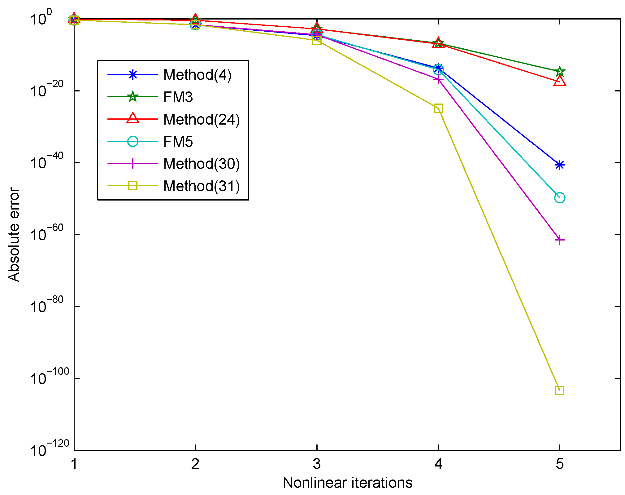The iterative processes of the iterative methods are given by Figure 1, Figure 2, Figure 3, Figure 4 and Figure 5.

Table 1. Numerical results of different iterative methods for Problem 1.

Methods	NIT	EVL	FU	ACOC
(4)	7	7.931$\times {10}^{-126}$	2.395$\times {10}^{-374}$	3.00000
FM3	7	6.263$\times {10}^{-153}$	2.601$\times {10}^{-416}$	2.73574
(24)	7	5.070$\times {10}^{-180}$	3.909$\times {10}^{-538}$	3.00000
FM5	6	6.709$\times {10}^{-344}$	4.721$\times {10}^{-1374}$	3.98043
(30)	6	3.068$\times {10}^{-415}$	1.153$\times {10}^{-1892}$	4.56599
(31)	5	1.667$\times {10}^{-135}$	3.865$\times {10}^{-674}$	5.00108

Table 2. Numerical results of different iterative methods for Problem 2.

Methods	NIT	EVL	FU	ACOC
(4)	8	1.094$\times {10}^{-117}$	1.999$\times {10}^{-347}$	3.00000
FM3	7	2.310$\times {10}^{-147}$	8.319$\times {10}^{-401}$	2.74317
(24)	7	3.056$\times {10}^{-172}$	3.356$\times {10}^{-513}$	3.00000
FM5	6	8.076$\times {10}^{-373}$	2.939$\times {10}^{-1486}$	4.08488
(30)	5	1.821$\times {10}^{-108}$	2.669$\times {10}^{-497}$	4.79681
(31)	5	5.055$\times {10}^{-110}$	3.685$\times {10}^{-544}$	4.99999

Table 3. Numerical results of different iterative methods for Problem 3.

Methods	NIT	EVL	FU	T	ACOC
(4)	5	5.500$\times {10}^{-123}$	5.095$\times {10}^{-373}$	567.141	3.00009
FM3	6	2.718$\times {10}^{-168}$	1.667$\times {10}^{-463}$	405.072	2.71295
(24)	6	6.628$\times {10}^{-234}$	8.935 $\times {10}^{-706}$	411.702	3.00001
FM5	5	5.078$\times {10}^{-292}$	8.678$\times {10}^{-1171}$	502.058	4.04268
(30)	5	9.412$\times {10}^{-376}$	2.431$\times {10}^{-1716}$	484.133	4.55973
(31)	4	4.154$\times {10}^{-113}$	1.123$\times {10}^{-570}$	377.491	5.01082

Table 4. Numerical results of different iterative methods for Problem 4.

Methods	NIT	EVL	FU	T	ACOC
(4)	6	4.082$\times {10}^{-122}$	3.486$\times {10}^{-365}$	57.127	3.00008
FM3	8	1.345$\times {10}^{-203}$	7.061$\times {10}^{-491}$	58.625	2.41965
(24)	7	1.185$\times {10}^{-114}$	1.976$\times {10}^{-299}$	52.385	2.70456
FM5	6	8.223$\times {10}^{-177}$	1.566$\times {10}^{-629}$	65.614	3.54447
(30)	6	1.601$\times {10}^{-229}$	1.857$\times {10}^{-852}$	65.099	3.74370
(31)	5	3.550$\times {10}^{-104}$	9.284$\times {10}^{-439}$	52.054	4.14892

Table 5. Numerical results of different iterative methods for Problem 5.

Methods	NIT	EVL	FU	ACOC
(4)	5	3.143$\times {10}^{-102}$	6.433$\times {10}^{-305}$	2.99114
FM3	6	2.325$\times {10}^{-168}$	3.396$\times {10}^{-459}$	2.71541
(24)	6	5.172$\times {10}^{-240}$	7.518$\times {10}^{-719}$	2.98298
FM5	5	8.133$\times {10}^{-292}$	2.547$\times {10}^{-1163}$	4.05479
(30)	5	2.915$\times {10}^{-369}$	2.206$\times {10}^{-1684}$	4.56718
(31)	4	1.441$\times {10}^{-102}$	3.107$\times {10}^{-511}$	4.99898

Table 6. Numerical results of different methods for Problem 6 (n = 10).

Methods	(4)	FM3	(24)	FM5	(30)	(31)
$NIT$	5	6	6	4	4	4
$e-Time$	47.654	48.297	47.533	48.048	47.861	47.851

Figure 1. The iterative processes of iterative methods for Problem 1.

Figure 2. The iterative processes of iterative methods for Problem 2.

Figure 3. The iterative processes of iterative methods for Problem 3.

Figure 4. The iterative processes of iterative methods for Problem 4.

Figure 5. The iterative processes of iterative methods for Problem 5.

Problem 1.

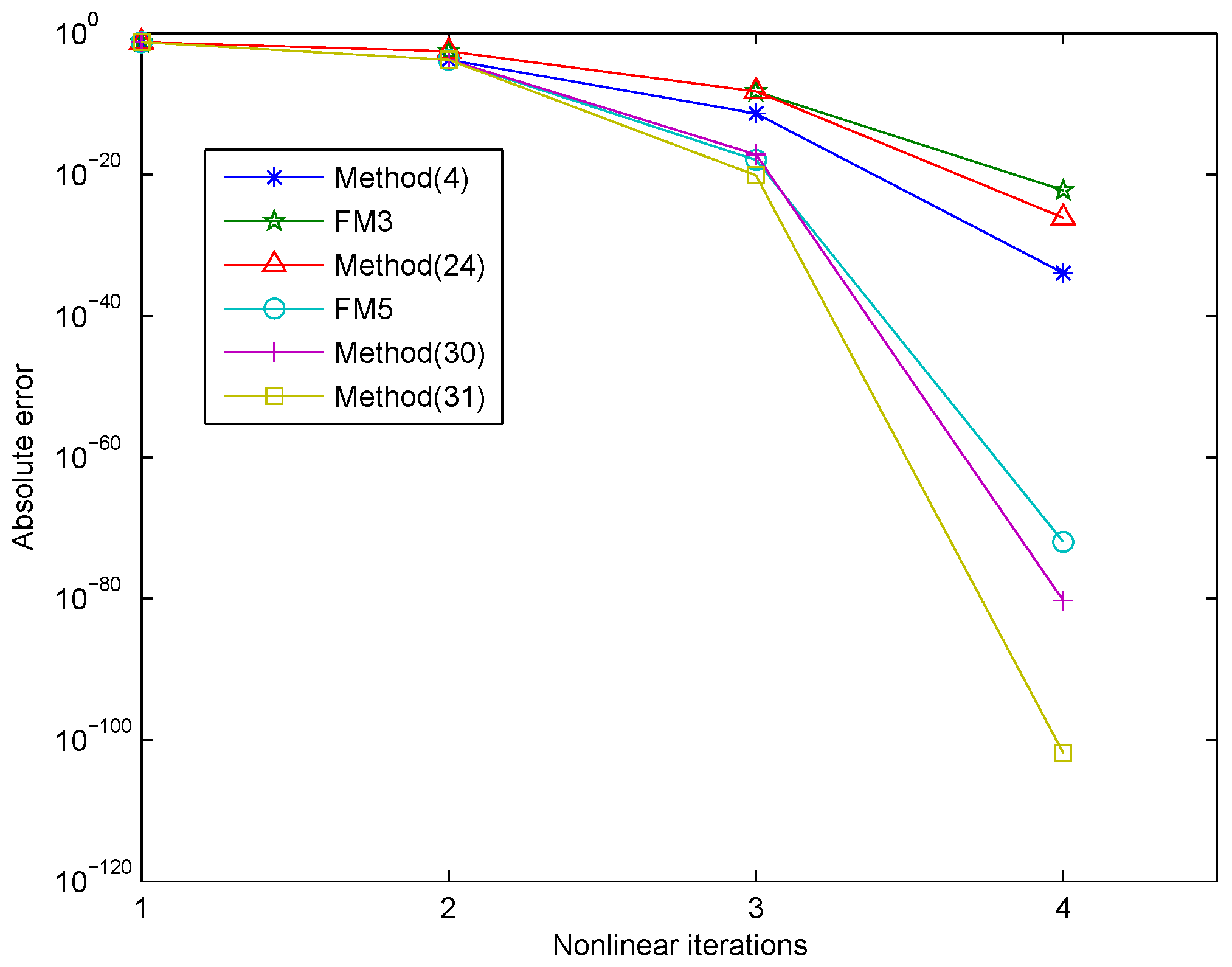
$$\left\{\begin{array}{c}{t}_i^2{t}_{i+1}-1=0,1\le i\le 19,\\ t_{20}^2{t}_1-1=0.\end{array}\right.$$

The solution of problem 1 is $\eta ={\{1,1,\cdots ,1\}}^T$ and the initial value is $t^{(0)}={\{1.25,1.25,\cdots ,1.25\}}^T$.

Figure 1 shows that the method in (31) had higher accuracy than the other methods. The accuracy of the method in (24) was similar to that of the FM3 method for Problem 1.

Problem 2.

$$2t_i^2-2\left(\sum _{j=1}^{20}{t}_j^2\right)+arctan{t}_i=-1,i=1,2,\cdots 20.$$

The solution of Problem 2 is $\eta \approx {(0.175768,\cdots ,0.175768)}^T$ and the initial guess is $t^{(0)}={(0.1,\cdots 0.1)}^T.$

Figure 2 shows that the methods in (30) and (31) had higher accuracy than the other methods. The method in (30) and (31) had similar convergence behaviors for Problem 2. The accuracy of the method in (24) was similar to that of the FM3 method for Problem 2.

Problem 3.

ODE problem [13]:

$$\begin{array}{c}{z}^{″}(t)=-\alpha e^{z(t)},t\in [0,1],\\ z(0)=0,z(1)=1.\end{array}$$

Using the discretization method in this problem, we obtain

$$\begin{array}{c}{z}_{k-1}-2z_k+z_{k+1}+\alpha h^2{e}^{z_k}=0,k=1,2,3,\dots ,n-1.\end{array}$$

For $n=101,$ we chose the initial value $z^{(0)}={(0.500,0.500,\cdots ,0.500)}^T$ and obtained the solution ${(0.00539,0.02168,0.01587,\dots ,0.00539)}^T$. The numerical results are shown in Table 3.

Figure 3 shows that our method, shown in (31), had higher accuracy than the other methods under the same number of iterations.

Problem 4.

ODE problem [14]:

$$\begin{array}{c}{z}^{″}(t)=z{(t)}^3+sin(z^{\prime }{(t)}^2),t\in [0,1],\\ z(0)=0,z(1)=1.\end{array}$$

The interval $[0,1]$ was partitioned into n intervals with a step size of $h=1/n$. Using the difference method to discrete the derivative, we obtained

$$\begin{array}{c}{z}_k^{″}=\frac{z_{k+1}-2z_k+z_{k-1}}{h^2},k=1,2,3,\cdots ,n-1,\end{array}$$

and

$$\begin{array}{c}{z}_k^{\prime }=\frac{z_{k+1}-z_{k-1}}{2h},k=1,2,3,\cdots ,n-1.\end{array}$$

We obtained

$$\begin{array}{c}{z}_{k-1}-2z_k+z_{k+1}-h^2{z}_k^3-h^{2}sin({(\frac{z_{k-1}-z_{k+1}}{2h})}^2)=0,k=1,2,3,\dots ,n-1.\end{array}$$

For $n=20$, we chose the initial value $t^{(0)}={(0.5,\cdots 0.5)}^T$ and obtained the solution $(0.0314264,$ ${0.063837,0.0972935,\dots ,0.926986)}^T$. The numerical results are shown in Table 4.

Problem 5.

$$\left\{\begin{array}{c}{x}_1^{3/2}-x_2-\frac{3}{4}+0.005|x_1-1|=0\\ x_2^{3/2}-\frac{2}{9}{x}_2-\frac{3}{8}+0.005\left|x_1\right|=0.\end{array}\right.$$

The solution is $\eta ={\{1.0207,0.27988\}}^T$ and the initial value is $x^{(0)}={\{0.9638,0.2376\}}^T$.

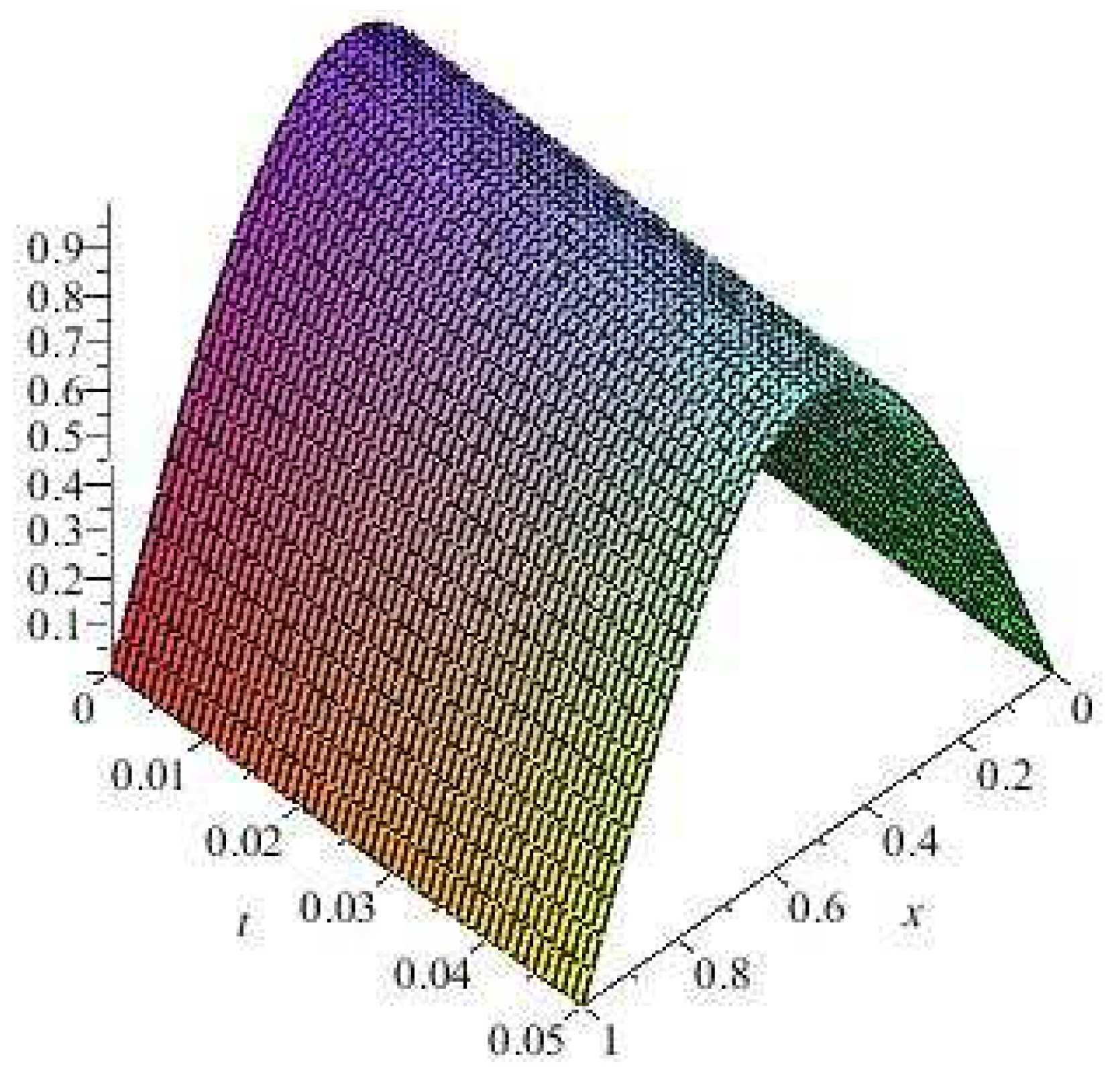
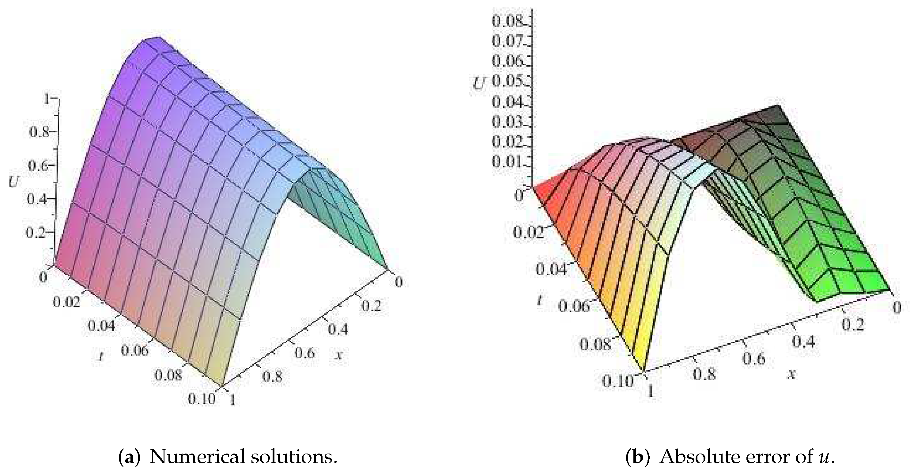
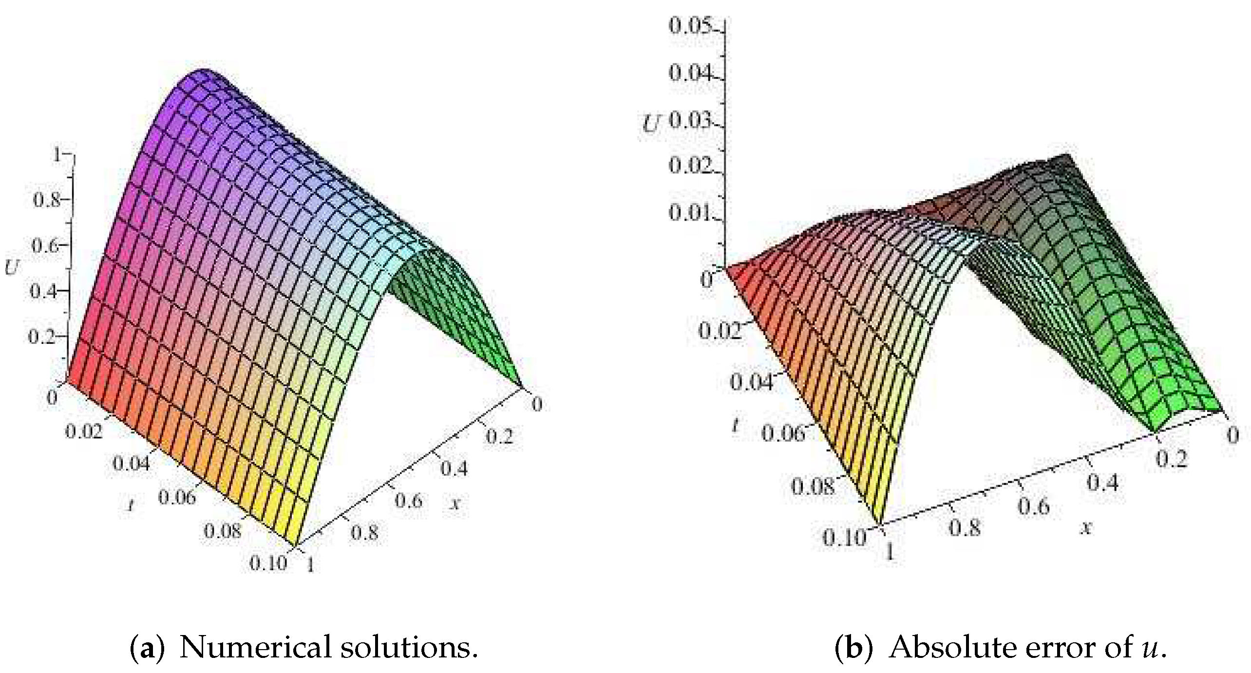
Problem 6.

Heat conduction problem [15]:

$$\begin{array}{c}{z}_{xx}=z_t+z_x-z^2+f(x,t),x\in [0,1],t\ge 0,\\ z(1,t)=0,z(0,t)=0.\\ f(x,t)=((2-{\pi }^2)sin(\pi x)-\pi cos(\pi x))e^{(-t)}\end{array}$$

This problem was transformed into nonlinear systems. The step size for t was $h=1/N$ and the step size for x was $k=T/N$. Let $z_{i,j}\approx z(x_i,t_j)$, $z_x(x,t)\approx \frac{z(x+h,t)-z(z-h,t)}{2h}$, $z_t(x,t)\approx \frac{z(x,t)-z(x,t-k)}{k}$ and $z_{xx}(x,t)\approx \frac{z(x+h,t)-2z(x,t)+z(x-h,t)}{h^2}$; we obtained

$$\begin{array}{c}(-2h^2-4k)z_{i,j}+(kh+2k)z_{i-1,j}+(2k-kh)z_{i+1,j}+2k{h}^2{z}_{i,j}^2-2k{h}^{2}f(t_i,x_j)+2h^2{z}_{i,j-1}=0\end{array}$$

The numerical results are given in Table 6. The exact solution $z(x,t)=exp(-t)sin(\pi x)$ of this problem is shown in Figure 6. The absolute value of error of the solution and approximate solution obtained using the method in (31) are shown in Figure 7 and Figure 8.

Figure 6. The exact solutions of Example 6.

Figure 7. Numerical solutions (a) of Example 6 (n = 10) produced by the method (b) in (31).

Figure 8. Numerical solutions (a) of Example 6 (n = 20) produced by the method (b) in (31).

4. Dynamical Analysis

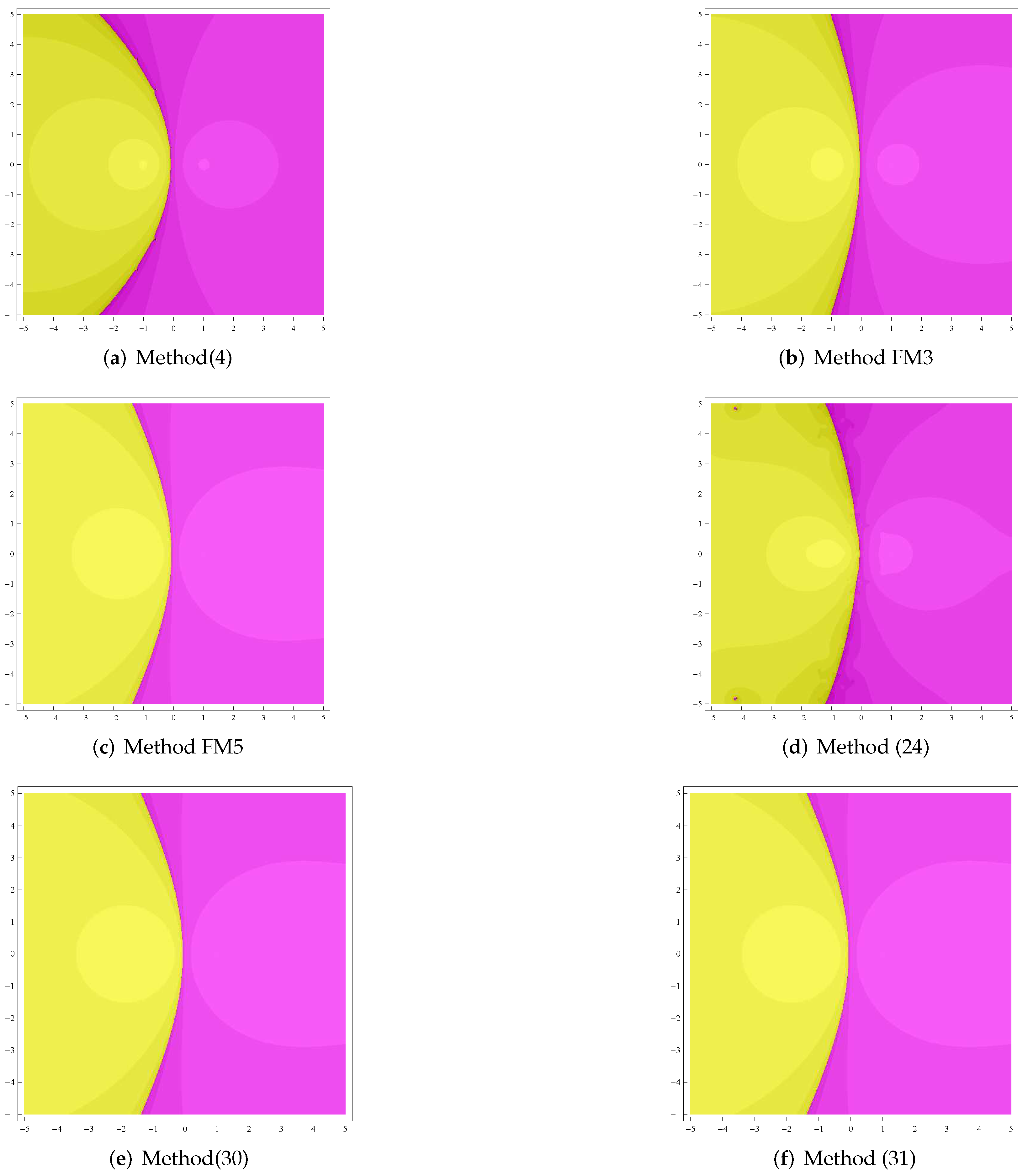
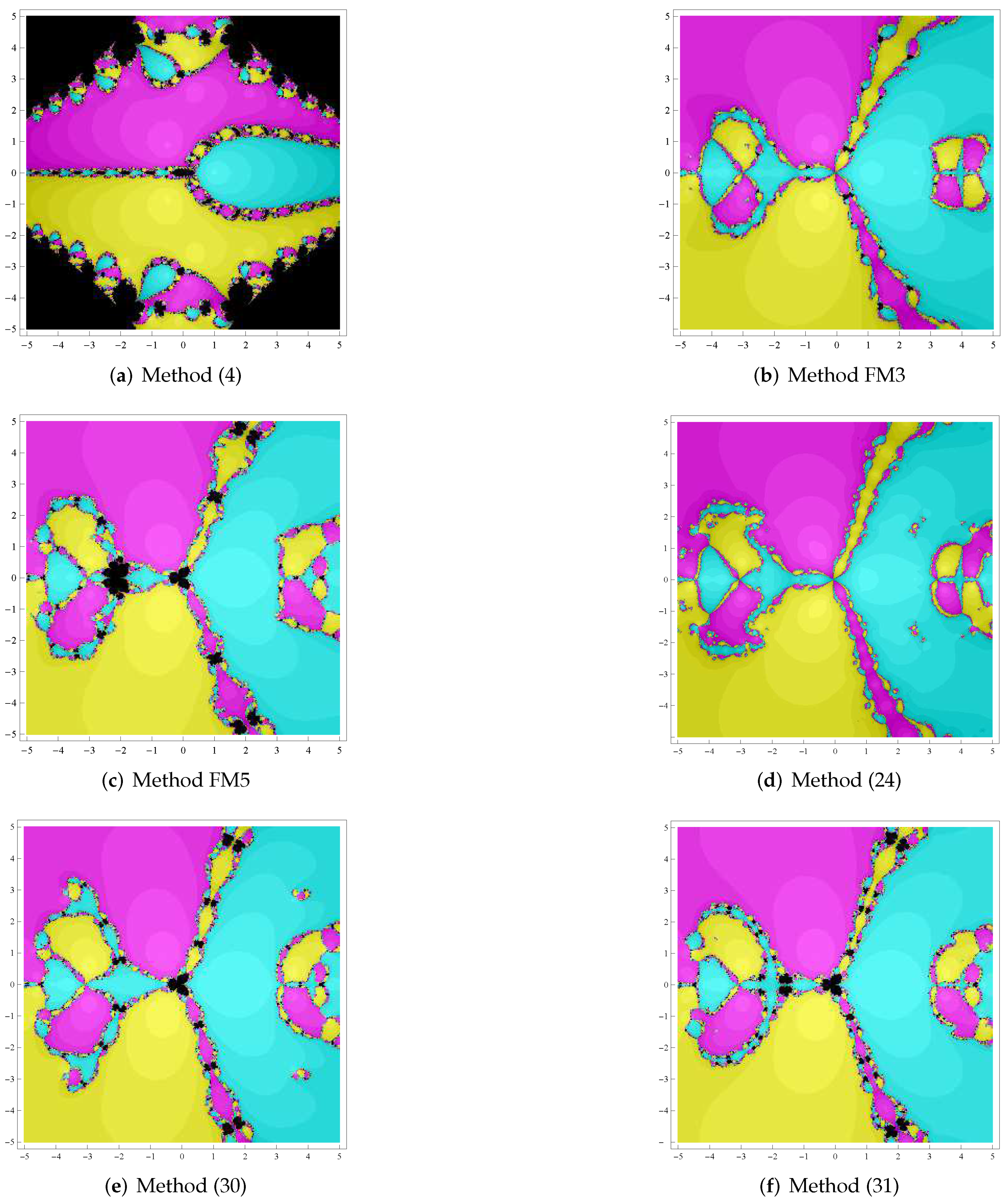
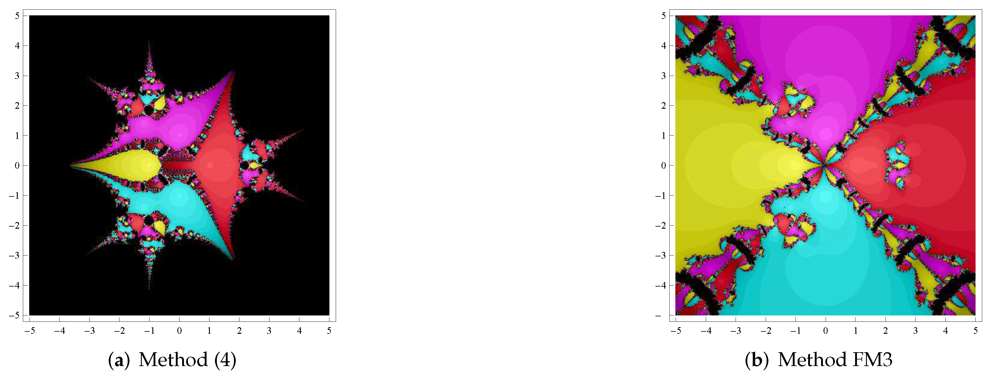
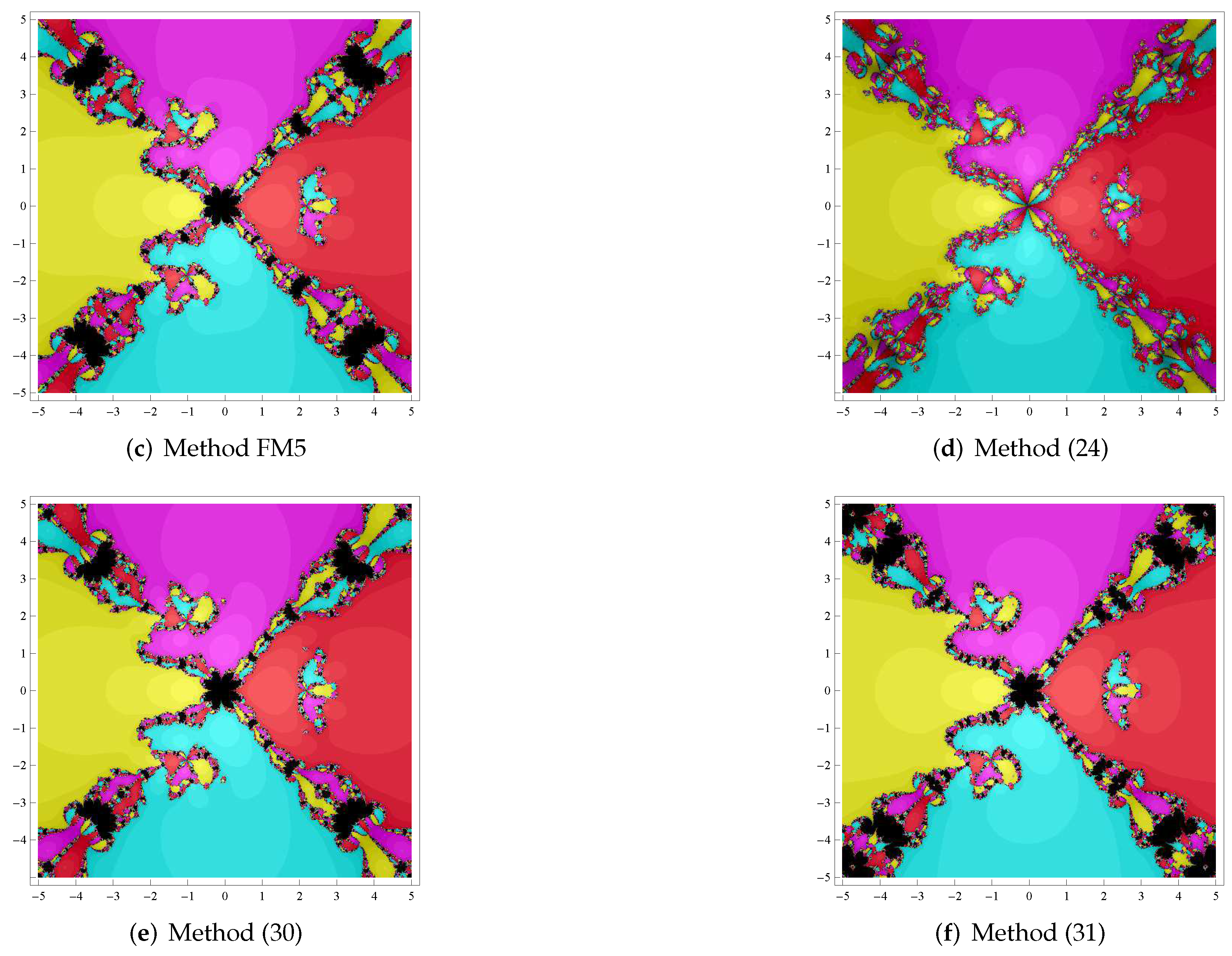
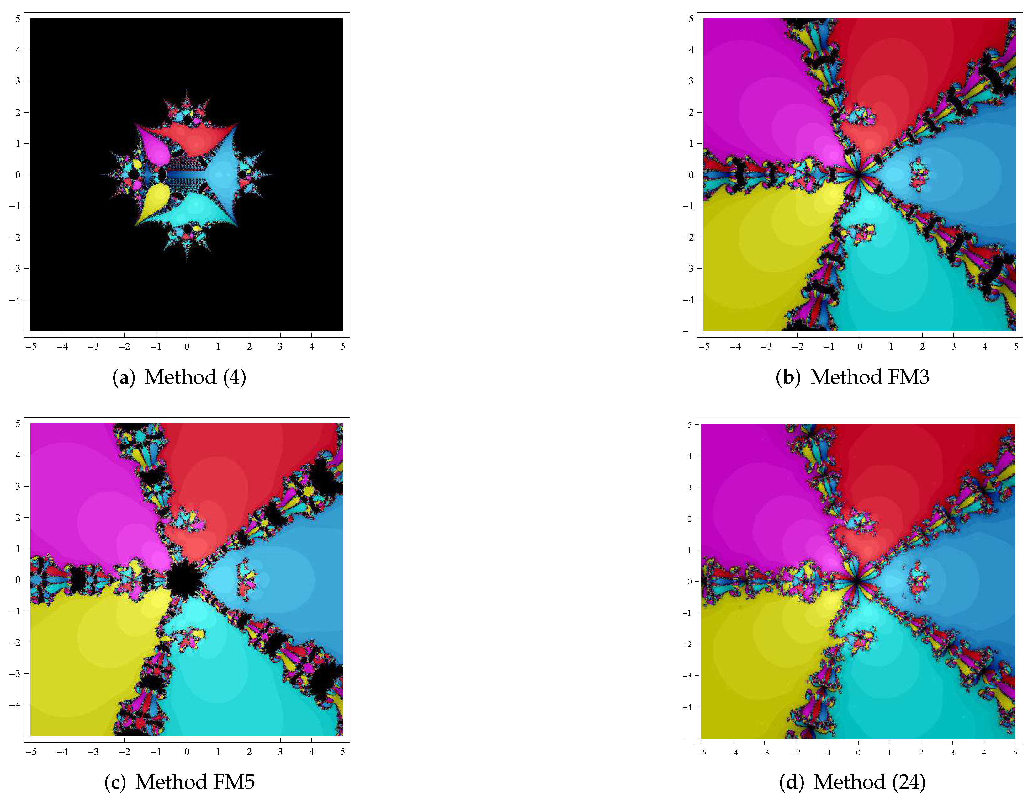
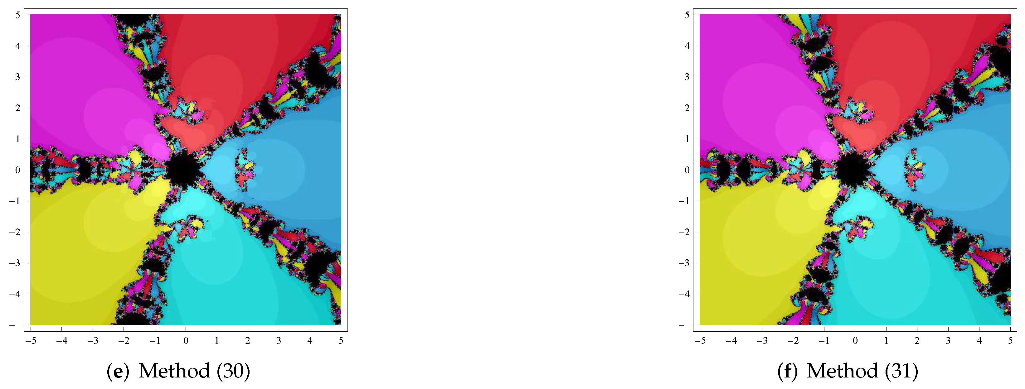
Recently, the dynamical analysis method has been applied to study the stability of the iterative method. Some basic concepts on complex dynamics can be found in references [16,17,18,19,20,21,22,23,24]. For brevity, we omit these concepts in this section. If an iterative method has good stability, it must has good properties for solving simple nonlinear equations. So, we compared our methods with other methods for solving complex equations $z^n-1=0,$$(n=2,3,4,5)$. The field $D=[-5.0,5.0]\times [-5.0,5.0]\in C$ was divided into a grid of $500\times 500$. If the initial point $z_0$ did not converge to the zero of the function after 25 iterations, it was painted with black. The tolerance $|z-z^{*}|<{10}^{-3}$ was used in our programs. Table 7, Table 8, Table 9 and Table 10 show the computing time (Time) for drawing the dynamical planes and the percentage of points (POPs) which guaranteed the convergence to the roots of the complex equations $z^n-1=0,$$(n=2,3,4,5)$.

Table 7. Numerical results of different methods for $z^2-1=0$.

Methods	(4)	FM3	FM5	(24)	(30)	(31)
$POP$	99.99 %	100%	100%	100%	100%	100%
$Time$	38.87	40.86	39.34	42.42	38.66	38.05

Table 8. Numerical results of different methods for $z^3-1=0$.

Methods	(4)	FM3	FM5	(24)	(30)	(31)
$POP$	68.53%	99.45%	97.25%	99.96%	97.96%	97.70%
$Time$	91.04	57.38	61.09	59.27	59.28	56.58

Table 9. Numerical results of different methods for $z^4-1=0$.

Methods	(4)	FM3	FM5	(24)	(30)	(31)
$POP$	21.72%	92.93%	91.89%	99.31%	92.65%	89.45%
$Time$	159.96	87.82	92.12	99.70	99.87	87.80

Table 10. Numerical results of different methods for $z^5-1=0$.

Methods	(4)	FM3	FM5	(24)	(30)	(31)
$POP$	10.48%	92.96%	89.51%	97.95%	89.38%	90.33%
$Time$	179.48	92.63	97.92	92.10	96.96	92.08

Figure 9, Figure 10, Figure 11 and Figure 12 show that our method, shown in (24), is the most stable method and the stability of the method in (4) without memory is the worst among the tested methods.

Figure 9. Dynamical planes for $z^2-1=0$. (a) Method (4), (b) Method FM3, (c) Method FM5, (d) Method (24), (e) Method (30), (f) Method (31).

Figure 10. Dynamical planes for $z^3-1=0$. (a) Method (4), (b) Method FM3, (c) Method FM5, (d) Method (24), (e) Method (30), (f) Method (31).

Figure 11. Dynamical planes for $z^4-1=0$. (a) Method (4), (b) Method FM3, (c) Method FM5, (d) Method (24), (e) Method (30), (f) Method (31).

Figure 12. Dynamical planes for $z^5-1=0$. (a) Method (4), (b) Method FM3, (c) Method FM5, (d) Method (24), (e) Method (30), (f) Method (31).

Table 7, Table 8, Table 9 and Table 10 show that, compared with other methods, the method in (24) had the highest percentage of points which guaranteed the convergence to the roots of the complex equations and the method in (31) costed the least computing time.

5. Conclusions

In this paper, three Kurchatov-type accelerating iterative schemes with memory were obtained by using two novel Kurchatov-type divided difference operator. The new methods avoided the evaluation of the derivative. The orders of convergence of our methods, shown in (24), (30) and (31), are 3, $(5+\sqrt{17})/2\approx 4.56$ and 5, respectively. We also corrected the order of convergence of Chicharro’s methods, FM3 and FM5. In experimental application, our methods were applied to nonlinear ODEs and PDEs. The numerical results show that, compared with other methods, our methods, shown in (30) and (31), had higher computational accuracy. Dynamical planes were used to analyze the stability of the presented methods. It is worth noting that our method with memory, shown in (24), had better stability than the other methods in this paper. The stability of the method without memory in (4) was the worst. We can conclude that iterative methods with memory can effectively improve the stability of iterative methods without memory.