Article

A Novel Analytical Formula for the Discounted Moments of the ECIR Process and Interest Rate Swaps Pricing

by
Ratinan Boonklurb
1,
Ampol Duangpan
1,
Udomsak Rakwongwan
2,* and
Phiraphat Sutthimat
1
1
Department of Mathematics and Computer Science, Faculty of Science, Chulalongkorn University, Bangkok 10330, Thailand
2
Department of Mathematics, Faculty of Science, Kasetsart University, Bangkok 10900, Thailand
*
Author to whom correspondence should be addressed.
Fractal Fract. 2022, 6(2), 58; https://doi.org/10.3390/fractalfract6020058
Submission received: 7 December 2021 / Revised: 4 January 2022 / Accepted: 20 January 2022 / Published: 24 January 2022
(This article belongs to the Special Issue Fractional Dynamics: Theory and Applications)

Abstract

:
This paper presents an explicit formula of conditional expectation for a product of polynomial functions and the discounted characteristic function based on the Cox–Ingersoll–Ross (CIR) process. We also propose an analytical formula as well as a very efficient and accurate approach, based on the finite integration method with shifted Chebyshev polynomial, to evaluate this expectation under the Extended CIR (ECIR) process. The formulas are derived by solving the equivalent partial differential equations obtained by utilizing the Feynman–Kac representation. In addition, we extend our results to derive an analytical formula of conditional expectation of a product of mixed polynomial functions and the discounted characteristic function. The accuracy and efficiency of the proposed scheme are also numerically shown for various modeling parameters by comparing them with those obtained from Monte Carlo simulations. In addition, to illustrate applications of the obtained formulas in finance, analytical pricing formulas for arrears and vanilla interest rate swaps under the ECIR process are derived. The pricing formulas become explicit under the CIR process. Finally, the fractional ECIR process is also studied as an extended case of our main results.

1. Introduction

A conditional expectation has been widely used in many branches of science. It can be easily computed if the probability density function (PDF) is known. However, often, the densities are unknown or are in complicated forms. Let ( Ω , F t , { F t } 0 t T , Q ) be a filtered probability space generated by an adapted stochastic process { r t } 0 t T , where Ω is a sample space, Q is a risk-neutral measure and the family { F t } 0 t T of σ -field on Ω parametrized by t [ 0 , T ] is a filtration. This paper focuses on the conditional expectation of a nonlinear function of the form:
E Q r T γ e λ r T t T ( α r s + β ) d s r t = r ,
whose analytical formula has not been discovered, when α , λ , β , γ R and r t evolve according to the extended Cox–Ingersoll–Ross (ECIR) process [1] governed by the stochasic differential equation (SDE):
d r t = θ ( t ) μ ( t ) r t d t + σ ( t ) r t d W t ,
where W t is a Wiener process. The parameter θ corresponds to the speed of adjustment to the mean of the invariant distribution μ and the parameter σ determines the state space of the diffusion and the shape of the invariant distribution. The Cox–Ingersoll–Ross (CIR) process, which was first introduced by Feller [2], is a special case of the ECIR process when the parameters are constant. Both processes are commonly used to describe the dynamic of interest rates, see, e.g., [1,3]. However, many empirical evidence strongly indicates that the parameters should be time-dependent, see, e.g., [1,4,5].
The conditional expectation in this form has many useful applications. In finance, from the fundamental theorem of asset pricing, a no-arbitrage price at any time t of a derivative is a conditional expectation under a risk-neutral measure of its discounted payoff given its value at time t [6]. Thus, the valuation of financial derivatives such as zero-coupon bonds, interest rate swaps (IRSs), and options usually involves evaluating this form of a conditional expectation, see also Duffie et al.’s work in [7]. In 2004, under the assumption that interest rates follow the CIR process, Mallier and Alobaidi [8] derived analytical formulas for the two well-known types of IRSs, arrears and vanilla swaps by utilizing the inverse Laplace transform and the Green’s function. The formula is in an analytic expression for the arrears swap, but it is only in a mathematical expression for the vanilla swap. In 2015, Moreno and Platania [9] provided a mathematical formula for forward rate agreements (FRAs) under a special case of the ECIR process where the modeling parameters are in terms of sine and cosine functions [10], namely the cyclical square-root model. Recently, Thamrongrat and Rujivan [11] presented an analytical formula for pricing IRSs in terms of bond prices under the ECIR process. However, the formula was derived under a discrete discounted rate assumption. In other words, they derived an analytical expression for (1) when γ = α = β = 0 . In addition to derivative pricing in finance, this conditional expectation is also seen in the generalized method of the moments estimator used to calibrate the parameters’values of a process from discretely sampled data [12].
Dufresne [13], in 2001, successfully derived an analytical formula for the conditional moment E Q r T γ F t , which is a special case of the considered conditional expectation (1), for some γ R under the CIR process for the parameters satisfying some certain conditions by computing the process’s density function. The formula can be written in a closed form if γ N { 0 } . In 2016, the formulas in Dufresne’s work were extended to the ECIR process by Rujivan [14] by solving the partial differential Equation (PDE) derived by utilizing the Feynman–Kac representation. More recently, Sutthimat et al. [15] extended Rujivan’s work to derive an analytical formula for the conditional expectation of a product of polynomial and exponential functions E Q r T γ e λ r T F t for γ , λ R . One primary concern for the proposed formulas of [14,15] is that the coefficients in the formulas, which are in the integral forms, may not be analytically integrable. In that case, some numerical integration methods are required. By using a Lie algebra approach, Grasselli [16] can directly find an analytical formula of the conditional expectation (1) under CIR process for some α , λ , β and γ satisfying some certain conditions. However, their expressions were in terms of a product between the gamma functions and a confluent hypergeometric function 1 F 1 which is an infinite sum. This may be difficult to use in practice. To the best of our knowledge, the analytical formula for (1) is as yet unknown.
In this work, by utilizing the Feynman–Kac representation, we successfully derived an analytical formula for the expectation (1) under the ECIR process by solving the equivalent partial differential equation problem. The formula is in the closed form under the CIR process. Moreover, we extend the formula to the conditional expectation of a product of two polynomial and one exponential functions E Q r s n 1 r T n 2 e t T ( α r u + β ) d u r t = r , where α , β R , n 1 , n 2 N { 0 } and 0 t < s < T . We also proposed a numerical scheme, constructed from the finite integration method (FIM) with shifted Chebyshev polynomial [17,18], to evaluate the analytical formulas of the conditional expectations and verified its accuracy and efficiency. To illustrate its applications in finance, we derived the analytical formulas for two interest rate swaps, namely arrears and vanilla swaps under the ECIR process. Unlike those from [8], under the CIR process, the formulas for both swaps are in closed form. Finally, the fractional ECIR process is also studied as an extended case of our main results.
The rest of the paper is organized as follows. Section 2 gives a brief overview of the ECIR process. The key methodology as well as main theorems are provided in Section 3. Section 4 introduces the numerical method for numerically evaluating the analytical formulas and provides numerical validations for the formulas. The formulas for pricing the arrears and vanilla swaps are presented in Section 5. Section 6 provides a study case of the fractional ECIR process adopt the idea from our main results given in Section 3. Section 7 presents the conclusions and discussions.

2. The Extended Cox–Ingersoll–Ross Process

For the ECIR process (2), in order to confirm that there exists a path-wise unique strong solution for the process r t in (2) and to avoid zero almost everywhere with respect to the probability measure Q for all t [ 0 , T ] , the two following assumptions studied by Maghsoodi [5] are needed (see details in Theorems 2.1 and 2.4 of their work). Altogether, we need the following sufficient condition.
Assumption 1
([5]). The time dependent parameters θ ( t ) , μ ( t ) and σ ( t ) in the ECIR process (2) are smooth and strictly positive, μ ( t ) σ 2 ( t ) is locally bounded on [ 0 , T ] and 2 θ ( t ) μ ( t ) σ ( t ) 2 .
It is worth noting that the CIR process is a special case of the ECIR process in which the parameters are constants and the Assumption 1 still holds for this case.
To achieve our aim, one fundamental question arises: Why do we not use the CIR process’s transition PDF directly? It is known that its transition PDF has the expression in terms of Bessel function of the first kind of order q, see [19,20], that is:
p r , T r t , t = c τ e ( u + v ) v u q / 2 I q 2 u v ,
where τ = T t , c τ = 2 θ σ 2 1 e θ τ , u = c τ r t e θ τ , v s . = c τ r , q = 2 θ μ σ 2 1 and I q ( · ) is the Bessel function of the first kind of order q. As displayed above, since the CIR process’s transition PDF is very complicated, the closed-form formulas for the conditional expectation (1) by applying this transition PDF are unavailable or complicated as well.
The situation becomes even more complicated for the ECIR process case; for instance, the ECIR ( d ) process presented by Egorov et al. [21]. Its dynamics are governed by the following time-inhomogeneous diffusion process:
d r t = θ σ 0 2 d 4 θ e 2 σ 1 t r t d t + σ 0 e σ 1 t r t d W t ,
where θ , σ 0 are positive, σ 1 is a real and d is positive constant with the transition PDF
p r , T r t , t = 1 2 G e λ + G r 2 G r λ d 2 4 I d 2 1 λ G r .
Here, λ = r t v , G = e θ τ v , v = 8 σ 1 σ 0 2 e θ τ e 2 σ 1 T e 2 σ 1 t , τ = T t and again I q ( · ) is the Bessel function of the first kind. This transition PDF was first proposed by Maghsoodi [5]. To avoid using the transition PDF for calculating (1), we employ the Feynman–Kac representation. This representation offers a method of solving a conditional expectation of an Itô random process by deterministic methods. In fact, it provides a relation between an Itô random process and a PDE.

3. Main Results

In this section, we present the methodology used in this paper as well as the main results. Theorem 1 gives an analytical formula for the conditional expectation of a product of polynomial and exponential functions, E Q r T γ e λ r T t T ( α r s + β ) d s r t = r where r t follows the ECIR process and α , λ , β , γ R . Theorem 2 is a special case of Theorem 1 when γ is a non-negative integer. In such case, the infinite sum, which can potentially cause a truncation error in practice, can be reduced into a finite sum. It should be mentioned that our proposed formulas for the ECIR process are more general and cover the results given in [14,15,16,22]. The analytical formulas presented in Theorems 1 and 2 involve the computation of the solution of the Riccati differential equation. As the solution of such equation does not have an analytical form except for some special cases, such as when α = 0 , we propose a very efficient numerical approach to solve the equation in Section 4.
Theorem 1.
Suppose that r t follows the ECIR process (2) with α, λ, β, γ R . Let 0 t T . Then,
U E γ ( r , τ ) : = E Q r T γ e λ r T t T ( α r s + β ) d s r t = r = e r B ( τ ) j = 0 A j γ ( τ ) r γ j ,
for all ( r , τ ) D E γ ( 0 , ) × [ 0 , ) , where τ = T t 0 . Moreover, the infinite series in (3) converges uniformly on D E γ . The coefficients in (3) can be expressed by:
A 0 γ ( τ ) = e 0 τ P 0 ( ξ ) d ξ and A j γ ( τ ) = e 0 τ P j ( ξ ) d ξ 0 τ e 0 ξ P j ( η ) d η Q j ( ξ ) A j 1 γ ( ξ ) d ξ ,
for j N , where
P j ( ξ ) = θ ( T ξ ) μ ( T ξ ) + ( γ j ) σ 2 ( T ξ ) B ( ξ ) ( γ j ) θ ( T ξ ) β and Q j ( ξ ) = ( γ j + 1 ) θ ( T ξ ) μ ( T ξ ) + 1 2 ( γ j ) σ 2 ( T ξ ) .
The function B is obtained by solving the Riccati differential equation
B ( ξ ) = 1 2 σ 2 ( T ξ ) B 2 ( ξ ) θ ( T ξ ) B ( ξ ) α , B ( 0 ) = λ .
Proof. 
Under the uniformly convergent assumption, the Feynman–Kac representation is applied to solve U : = U E γ ( r , τ ) in (3) which satisfies the corresponding PDE [23],
U τ + θ ( T τ ) μ ( T τ ) r U r + r 2 σ 2 ( T τ ) U r r α r + β U = 0 ,
where the initial condition at τ = 0 is given by:
U E γ ( r , 0 ) = E Q r T γ e λ r T T T ( α r s + β ) d s | r T = r = r γ e λ r .
Then, we compare the coefficients in (3) and (8) to obtain the conditions B ( 0 ) = λ , A 0 γ ( 0 ) = 1 and A j γ ( 0 ) = 0 for j N . Next, we find the partial derivatives U τ , U r and U r r by using (3) which are:
U τ = e r B ( τ ) j = 0 d d τ A j γ ( τ ) r γ j + d d τ B ( τ ) A j γ ( τ ) r γ j + 1 , U r = e r B ( τ ) j = 0 ( γ j ) A j γ ( τ ) r γ j 1 + B ( τ ) A j γ ( τ ) r γ j and U r r = e r B ( τ ) j = 0 ( γ j ) ( γ j 1 ) A j γ ( τ ) r γ j 2 + 2 ( γ j ) B ( τ ) A j γ ( τ ) r γ j 1 + B 2 ( τ ) A j γ ( τ ) r γ j .
Now, these above partial derivatives and U in (3) are substituted into (7) by letting A j : = A j γ ( τ ) and B : = B ( τ ) . Thus, (7) becomes:
0 = e r B j = 0 A j r γ j + B A j r γ j + 1 + θ ( T τ ) μ ( T τ ) r e r B j = 0 ( γ j ) A j r γ j 1 + B A j r γ j + r 2 σ 2 ( T τ ) e r B j = 0 ( γ j ) ( γ j 1 ) A j r γ j 2 + 2 ( γ j ) B A j r γ j 1 + B 2 A j r γ j α r + β e r B j = 0 A j r γ j ,
which can be simplified by employing (5) as:
0 = A 0 B + θ ( T τ ) B 1 2 σ 2 ( T τ ) B 2 + α r γ + 1 A 0 P 0 ( τ ) A 0 + A 1 B + θ ( T τ ) B 1 2 σ 2 ( T τ ) B 2 + α r γ j = 1 A j P j ( τ ) A j Q j ( τ ) A j 1 + A j + 1 B + θ ( T τ ) B 1 2 σ 2 ( T τ ) B 2 + α r γ j .
Consider (9) as a power series in r. Since r 0 and the leading coefficient A 0 0 , (9) holds under the following nonlinear differential equation:
B + θ ( T τ ) B 1 2 σ 2 ( T τ ) B 2 + α = 0
with the initial condition B ( 0 ) = λ and the linear differential equations:
A 0 P 0 ( τ ) A 0 = 0 and A j P j ( τ ) A j Q j ( τ ) A j 1 = 0
with their initial conditions A 0 ( 0 ) = 1 and A j ( 0 ) = 0 for j N . This completes the proof and the solutions of those linear differential equations are given in (4). □
Theorem 2.
According to Theorem 1 with γ = n N { 0 } , we have
U E n ( r , τ ) = E Q r T n e λ r T t T ( α r s + β ) d s | r t = r = e r B ( τ ) j = 0 n A j n ( τ ) r n j ,
for all ( r , τ ) ( 0 , ) × [ 0 , ) and τ = T t 0 , where A j n ( τ ) is defined in (4) and B ( τ ) is the solution of (6).
Proof. 
Let γ = n N { 0 } . Consider (4) at the index j = n + 1 , we get A n + 1 n ( τ ) = 0 due to Q n + 1 = 0 by (5). From the recurrence relation (4), we have A j n ( τ ) = 0 for all integers j n + 1 . Consequently, the infinite sum (3) can be reduced to the finite sum (10). □
Theorem 3 shows that the formulas can be expressed in closed forms under the CIR process where all parameters θ ( t ) = θ , μ ( t ) = μ and σ ( τ ) = σ are constants. Theorem 4 extends the result (10) in Theorem 2 to derive an analytical formula for a product of two polynomial and one exponential functions E Q r T i 1 n 1 r T i n 2 e t T i ( α r u + β ) d u r t = r for some constants α , β R and non-negative integers n 1 , n 2 .
Theorem 3.
Suppose that r t follows the CIR process with α , β , λ R and γ = n N { 0 } . Let 0 t T . Then,
U C n ( r , τ ) : = E Q r T n e λ r T t T ( α r s + β ) d s | r t = r = e r B ( τ ) j = 0 n A j n ( τ ) r n j
for all ( r , τ ) ( 0 , ) × [ 0 , ) , where τ = T t 0 . The coefficients in (11) can be expressed by
A 0 n ( τ ) = H 0 ( τ ) and A j n ( τ ) = H j ( τ ) k = 1 j 2 Q k k e ρ τ 1 ρ e ρ τ + 1 + θ + λ σ 2 e ρ τ 1 j
for j N , where ρ = θ 2 + 2 α σ 2 ,
Q j = ( n j + 1 ) θ μ + 1 2 ( n j ) σ 2 and H j ( τ ) = exp θ 2 μ τ σ 2 β τ + n j + θ μ σ 2 ρ τ 2 ρ ρ e ρ τ + 1 + θ + λ σ 2 e ρ τ 1 2 n j + θ μ σ 2 .
In addition, the solution B of (6) can be solved explicitly as:
B ( τ ) = λ ρ ( e ρ τ + 1 ) + 2 α λ θ ( e ρ τ 1 ) ρ e ρ τ + 1 + θ + λ σ 2 e ρ τ 1 .
Proof. 
By considering (6) with θ ( t ) = θ , μ ( t ) = μ and σ ( τ ) = σ , the analytical solution for the Riccati differential Equation (6) is given in (14) where ρ = θ 2 + 2 α σ 2 . Then, we have
0 τ B ( ξ ) d ξ = 2 σ 2 ln 2 ρ e ρ + θ 2 τ ρ e ρ τ + 1 + θ + λ σ 2 e ρ τ 1 .
Thus, we obtain:
e 0 τ P j ( ξ ) d ξ = exp 0 τ θ μ + ( n j ) σ 2 B ( ξ ) ( n j ) θ β d ξ = exp θ 2 μ τ σ 2 β τ + n j + θ μ σ 2 ρ τ 2 ρ ρ e ρ τ + 1 + θ + λ σ 2 e ρ τ 1 2 n j + θ μ σ 2 ,
which are defined to be H j ( τ ) for j N { 0 } . By Theorem 1, A 0 n ( τ ) = e 0 τ P 0 ( ξ ) d ξ = H 0 ( τ ) and
A 1 n ( τ ) = H 1 ( τ ) 0 τ 1 H 1 ( ξ ) Q 1 A 0 n ( ξ ) d ξ = 2 H 1 ( τ ) Q 1 e ρ τ 1 ρ e ρ τ + 1 + θ + λ σ 2 e ρ τ 1 .
From the result presented in (4) for j N , we obtain:
A j n ( τ ) = H j ( τ ) 0 τ 1 H j ( ξ ) Q j A j 1 n ( ξ ) d ξ = H j ( τ ) 0 τ 1 H j ( ξ ) Q j H j 1 ( ξ ) k = 1 j 1 2 Q k k e ρ u 1 ρ e ρ τ + 1 + θ + λ σ 2 e ρ τ 1 j 1 d ξ = H j ( τ ) k = 1 j 2 Q k k e ρ τ 1 ρ e ρ τ + 1 + θ + λ σ 2 e ρ τ 1 j .
Under the uniformly convergent assumption, the proof is completed. □
Theorem 4.
Suppose that r t follows the ECIR process (2) with β, γ R and n 1 , n 2 N { 0 } . Let 0 t < s < T . Then, we have
U E n 1 , n 2 r , τ 1 , τ 2 = E Q r s n 1 r T n 2 e t T ( α r u + β ) d u r t = r = e r B τ 1 ; B τ 2 ; 0 j = 0 n 2 k = 0 n 1 + n 2 j A j n 2 τ 2 ; B τ 2 ; 0 A k n 1 + n 2 j τ 1 ; B τ 1 ; B τ 2 ; 0 r n 1 + n 2 j k
for all ( r , τ 1 , τ 2 ) ( 0 , ) 3 , where τ 1 = s t , τ 2 = T s , B ( τ ; x ) is a solution of the Riccati differential Equation (6) with the initial condition B ( 0 ) = x , and A j γ ( τ ; B ) are coefficients described in (4).
Proof. 
By using the tower property for 0 t < s < T and applying the proposed Formula (10) twice, the conditional expectation (17) can be expressed by:
U E n 1 , n 2 r , τ 1 , τ 2 = E Q r s n 1 e t s ( α r u + β ) d u E Q r T n 2 e s T ( α r u + β ) d u r s r t = r = j = 0 n 2 A j n 2 τ 2 ; B τ 2 ; 0 E Q r s n 1 + n 2 j e r s B τ 2 ; 0 t s α r u + β d u r t = r = e r B τ 1 ; B τ 2 ; 0 j = 0 n 2 k = 0 n 1 + n 2 j A j n 2 τ 2 ; B τ 2 ; 0 A k n 1 + n 2 j τ 1 ; B τ 1 ; B τ 2 ; 0 r n 1 + n 2 j k
as required. □
Remark 1.
We can see that various statistics such as the first and second conditional moments, variances, mixed moments, covariances and correlations, can be derived as special cases of Theorem 4 where λ = α = β = 0 . This corresponds to Rujivan’s result [14]. As the maximum likelihood cannot be solved directly under ECIR, conditional moments are essential for parameter estimating methods such as the martingale estimating functions, generalized method of moments, and quasi-likelihood method.
Corollary 1.
Suppose that r t follows the ECIR process (2), n N and τ = T t 0 , we have
μ n ( r , τ ) : = E Q r T E r T r t n e t T ( α r u + β ) d u r t = r = j = 0 n n j U E j ( r , τ ) V E 1 ( r , τ ) n j ,
where V E n ( r , τ ) denotes U E n ( r , τ ) when λ = α = β = 0 . Note that, without the exponential term, this corresponds to central moments and is a conditional variance for n = 2 .
Proof. 
It is obtained directly by using the Binomial theorem together with Theorem 2. □
Remark 2.
Results above can be extended to approximate the expectation of any real analytic functions f of a random variable on an open interval, where its Taylor expansion at x 0 converges pointwise to f. For example, consider f ( x ) = x which can be expressed using Taylor expansion as:
x = x 0 + x x 0 2 x 0 ( x x 0 ) 2 8 x 0 3 + O ( x 3 ) .
By substituting x = r T and x 0 = E Q r T r t = r where r t follows the ECIR process for 0 t T and taking the conditional expectation, we have that
E Q r T e t T ( α r u + β ) d u r t = r V E 1 ( r , τ ) U E 0 ( r , τ ) + μ 1 ( r , τ ) 2 V E 1 ( r , τ ) μ 2 ( r , τ ) 8 V E 1 ( r , τ ) 3 .
The above expansion can be applied to other functions, such as exponential, logarithmic or trigonometric functions. However, one needs to make sure that the approximation converges as there is no empirical analysis providing the convergence condition of the Taylor expansions in a general stochastic context. Moreover, there is empirical evidence indicating that increasing the number of terms in Taylor approximation does not necessarily yield more accurate estimation. The classic example is given by Zhu and Lian [24]. They showed that a better accuracy of the convexity correction approximation (CCA), used to estimate volatility swap prices, cannot be achieved by extending the second-order Taylor expansion to that of the third order and gave the condition when CCA provides decent estimates.
Corollary 2.
Suppose that r t follows the ECIR process (2) and 0 t < s < T , we have:
Cov r s e t s ( α r u + β ) d u , r T e s T ( α r u + β ) d u r t = r = U E 1 , 1 r , τ 1 , τ 2 U E 1 ( r , τ 1 ) E Q r T e s T ( α r u + β ) d u r t = r ,
where τ 1 = s t and τ 2 = T s .
Proof. 
By using the definition of covariance, we have:
Cov r s e t s ( α r u + β ) d u , r T e s T ( α r u + β ) d u r t = r = E Q r s e t s ( α r u + β ) d u E Q r s e t s ( α r u + β ) d u r t r T e s T ( α r u + β ) d u E Q r T e s T ( α r u + β ) d u r t r t = E Q r s r T e t T ( α r u + β ) d u r t E Q r s e t s ( α r u + β ) d u r t E Q r T e s T ( α r u + β ) d u r t = U E 1 , 1 r , τ 1 , τ 2 U E 1 ( r , τ 1 ) E Q r T e s T ( α r u + β ) d u r t
as required. □
Remark 3.
The analytical form of E Q r T e s T ( α r u + β ) d u r t = r can be easily obtained using the tower property and Theorem 2.

4. Numerical Procedures

The analytical Formulas (3) and (17) in Theorems 1 and 4, respectively, used for pricing swaps under the ECIR process in Section 3, require the evaluation of the two parameters B ( τ ) and A j γ ( τ ) which are the functions of time variable τ . As we know, under the ECIR process, (6) cannot be solved for analytical solution. Thus, the analytical form of the two parameters cannot be obtained. In this section, we propose a very efficient scheme to numerically evaluate the formulas. The approach consists of two parts. The first part is to numerically solve the Riccati differential Equation (6) using the FIM base on the Chebyshev polynomials [25]. Then, the algorithms to evaluate the formulas are illustrated.

4.1. FIM with Shifted Chebyshev Polynomial

This subsection introduces the major tool for solving the Riccati differential equation, that is, the FIM based on the shifted Chebyshev polynomial. This numerical scheme was proposed by Boonklurb et al. [25] in 2018, which provided a very accurate solution using less computational nodes and, thus, an inexpensive consuming time. However, we adjust this method slightly by employing the shifted Chebyshev polynomials, in order to be easily applied to our considering domain of the Riccati differential equation, which is [ 0 , T ] where T > 0 .
Definition 1 describes the shifted Chebyshev polynomial. Its properties needed to construct the first and higher orders of the Chebyshev integration matrices, which are the main ingredients of the FIM, are detailed in Lemma 1.
Definition 1
([26]). The shifted Chebyshev polynomial of degree n 0 is defined by:
S n ( τ ) = cos n arccos 2 τ T 1 for τ [ 0 , T ] .
Lemma 1
([26]). The followings are properties of shifted Chebyshev polynomials.
(i) 
The zeros of shifted Chebyshev polynomial S n + 1 ( τ ) for τ [ 0 , T ] are
τ k = T 2 1 cos 2 k + 1 2 n + 2 π , k { 0 , 1 , 2 , , n } .
(ii) 
The single integrations of shifted Chebyshev polynomial S n ( τ ) for τ [ 0 , T ] are
S ¯ 0 ( τ ) = 0 τ S 0 ( ξ ) d ξ = τ , S ¯ 1 ( τ ) = 0 τ S 1 ( ξ ) d ξ = τ 2 T τ and S ¯ n ( τ ) = 0 τ S n ( ξ ) d ξ = T 4 S n + 1 ( τ ) n + 1 S n 1 ( τ ) n 1 2 ( 1 ) n n 2 1 , n 2 .
(iii) 
The shifted Chebyshev matrix S at each node τ k defined by(18)is
S = S 0 ( τ 0 ) S 1 ( τ 0 ) S n ( τ 0 ) S 0 ( τ 1 ) S 1 ( τ 1 ) S n ( τ 1 ) S 0 ( τ n ) S 1 ( τ n ) S n ( τ n ) .
Then, its multiplicative inverse is S 1 = 1 n + 1 diag 1 , 2 , 2 , , 2 S .
Next, the first order Chebyshev integration matrix is constructed. Let n N be a number of computational nodes. Assume that f ( τ ) is an approximate solution of any function which is defined by the linear combination of the shifted Chebyshev polynomials S 0 ( τ ) , S 1 ( τ ) , S 2 ( τ ) , , S n ( τ ) . Then, we have:
f ( τ ) = i = 0 n c i S i ( τ ) ,
where c i is an unknown coefficient to be considered. Let τ k be computational nodes that are generated by the zeros of the shifted Chebyshev polynomial S n + 1 defined by (18) in ascending order. After that, each node τ k is plugged into (19). Then, we obtain the following matrix form:
f ( τ 0 ) f ( τ 1 ) f ( τ n ) = S 0 ( τ 0 ) S 1 ( τ 0 ) S n ( τ 0 ) S 0 ( τ 1 ) S 1 ( τ 1 ) S n ( τ 1 ) S 0 ( τ n ) S 1 ( τ n ) S n ( τ n ) c 0 c 1 c n ,
which is denoted by f = S c . By Lemma 1(iii), we know that S is invertible. Thus, we get the coefficient c = S 1 f . Now, we consider a single-layer integration of f from 0 to τ k denoted by F ( τ k ) , we obtain:
F ( τ k ) = 0 τ k f ( ξ ) d ξ = i = 0 n c i 0 τ k S i ( ξ ) d ξ = i = 0 n c i S ¯ i ( τ k ) ,
where S ¯ i ( τ k ) for i { 0 , 1 , 2 , , n } are defined in Lemma 1(ii). As we substitute each nodal point τ k into the above equation, it can be written in the matrix form:
F ( τ 0 ) F ( τ 1 ) F ( τ n ) = S ¯ 0 ( τ 0 ) S ¯ 1 ( τ 0 ) S ¯ n ( τ 0 ) S ¯ 0 ( τ 1 ) S ¯ 1 ( τ 1 ) S ¯ n ( τ 1 ) S ¯ 0 ( τ n ) S ¯ 1 ( τ n ) S ¯ n ( τ n ) c 0 c 1 c n ,
which is denoted by F = S ¯ c = S ¯ S 1 f : = Jf , where J = S ¯ S 1 : = [ J k i ] is an ( n + 1 ) × ( n + 1 ) matrix representation for the integral operator called the Chebyshev integration matrix. Thus, the single-layer integration F ( τ k ) can be also expressed to another form as follows:
F ( τ k ) = 0 τ k f ( ξ ) d ξ = i = 0 n J k i f ( τ i ) .

4.2. Numerical Procedure for Theorem 1

Next, we utilize the FIM with the shifted Chebyshev polynomial to seek the numerical solution for the Riccati differential Equation (6) which is the initial value problem. First of all, let us recall the Riccati differential equation again,
B ( τ ) = 1 2 σ 2 ( T τ ) B 2 ( τ ) θ ( T τ ) B ( τ ) α , τ [ 0 , T ]
with initial condition B ( 0 ) = λ . To find its numerical formula, we discretize the domain [ 0 , T ] into n subintervals composed n + 1 nodes. These nodes are manufactured by the zeros of the shifted Chebyshev polynomial S n + 1 defined in (18), that are τ 0 < τ 1 < τ 2 < < τ n . By the idea of FIM, we have to transform the differential equation into the equivalent integral equation. Thus, to remove the derivative from (21), we take a single integral from 0 to τ k on both sides of (21). Then, we have:
B ( τ k ) = 1 2 0 τ k σ 2 ( T ξ ) B 2 ( ξ ) d ξ 0 τ k θ ( T ξ ) B ( ξ ) d ξ α τ k + C ,
where C is an arbitrary constant emerged in the process of integration. Subsequently, we apply the FIM based on the shifted Chebyshev polynomials to approximate the integral terms contained in (22) by using (20). We obtain:
B ( τ k ) = 1 2 i = 0 n J k i σ 2 ( T τ i ) B 2 ( τ i ) i = 0 n J k i θ ( T τ i ) B ( τ i ) α τ k + C .
Let σ i = σ ( T τ i ) and θ i = θ ( T τ i ) . As we vary the value of τ k for k { 0 , 1 , 2 , , n } by the zeros (18) into the above equation, we have the system of nonlinear equations which can be expressed to the matrix form:
B ( τ 0 ) B ( τ 1 ) B ( τ n ) = 1 2 J 00 J 01 J 0 n J 10 J 11 J 1 n J n 0 J n 1 J n n σ 0 2 B 2 ( τ 0 ) σ 1 2 B 2 ( τ 1 ) σ n 2 B 2 ( τ n ) J 00 J 01 J 0 n J 10 J 11 J 1 n J n 0 J n 1 J n n θ 0 B ( τ 0 ) θ 1 B ( τ 1 ) θ n B ( τ n ) α τ 0 τ 1 τ n + C 1 1 1 .
It can be simplified and denoted by:
B = 1 2 J Σ ( B B ) J Θ B α τ + C e ,
where J = S ¯ S 1 is the Chebyshev integration matrix described in the previous section, the notation ⊙ is the Hadamard product defined in [27] which means a product of elements in matrices at the same position and the other parameters contained in (23) are defined by the following:
Σ = diag σ 0 2 , σ 1 2 , σ 2 2 , , σ n 2 , Θ = diag θ 0 , θ 1 , θ 2 , , θ n , B = B ( τ 0 ) , B ( τ 1 ) , B ( τ 2 ) , , B ( τ n ) , τ = τ 0 , τ 1 , τ 2 , , τ n and e = 1 , 1 , 1 , , 1 has n + 1 components .
However, we see that (23) is in the matrix form of a nonlinear equation. Hence, the technique of linearization method is applied to (23) in order for convenient solving. Let m N , we then take the ( m 1 ) th and m th iterations into the variable B , which are, respectively, denoted by B m 1 and B m , for the nonlinear term in (23). The other terms are determined at the m th present iteration. Thus, (23) becomes
B m = 1 2 J Σ ( B m 1 B m ) J Θ B m α τ + C e ,
which can be rearranged to
1 2 J Σ diag B m 1 J Θ I B m + C e = α τ ,
where I is the ( n + 1 ) × ( n + 1 ) identity matrix and diag B m 1 is the diagonal matrix that diagonal entries are the elements of vector B m 1 . Moreover, we observe that C is the new unknown that occurred from the integration. Thus, we need to create one more equation by hiring the given initial condition B ( 0 ) = λ . Accordingly, we use (19) to transform this supplementary condition into the matrix form. Thus, at the m th iteration, we obtain:
λ = B ( 0 ) = i = 0 n c i S i ( 0 ) : = u c = u S 1 B m ,
where u = [ S 0 ( 0 ) , S 1 ( 0 ) , S 2 ( 0 ) , , S n ( 0 ) ] . Finally, we combine (24) and (25) to construct the iterative system of linear equations which has n + 2 unknowns as follows:
1 2 J Σ diag B m 1 J Θ I e u S 1 0 B m C = α τ λ .
Consequently, the iterative approximate solution B m can be sought by solving (26) in conjunction with an arbitrary initial guess of the iteration B 0 that makes the coefficient matrix to be invertible. Note that the stopping criterion for finding the m th iterative approximate solution B m is stopped when the m th error Euclidean norm ϵ m : = B m B m 1 of difference between the current and consecutively previous solutions is less than the given convergent tolerance T O L . Therefore, an approximate solution B ( τ ) at arbitrary point τ [ 0 , T ] can be estimated by:
B ( τ ) i = 0 n c i S i ( τ ) : = v c = v S 1 B m ,
where v = [ S 0 ( τ ) , S 1 ( τ ) , S 2 ( τ ) , , S n ( τ ) ] and B m is the m th terminal solution obtained by solving (26).
Now, we already have the approximate solutions B ( τ ) of the Riccati differential Equation (6) that will be used to estimate the coefficients A j γ ( τ ) for j N { 0 } contained in (4). Furthermore, we can also use the Chebyshev integration matrix J to represent the integral terms in (4). Thus, by applying (20) to (4), we have the estimated coefficients at the temporal variable τ k as follows:
A 0 γ ( τ k ) = exp 0 τ k P 0 ( u ) d u = exp i = 0 n J k i P 0 ( τ i ) = exp J k : P 0
and for j N ,
A j γ ( τ k ) = exp 0 τ k P j ( u ) d u 0 τ k exp 0 u P j ( s ) d s Q j ( u ) A j 1 γ ( u ) d u = exp i = 0 n J k i P j ( τ i ) i = 0 n J k i exp l = 0 n J i l P j ( τ l ) Q j ( τ i ) A j 1 γ ( τ i ) = exp J k : P j i = 0 n J k i exp J i : P j Q j ( τ i ) A j 1 γ ( τ i ) = exp J k : P j J k : exp J P j Q j A j 1 γ .
As the variables τ k for k { 0 , 1 , 2 , , n } are varied as the zeros (18) into these above two equations for A 0 γ and A j γ , we obtain:
A 0 γ = exp J P 0 and A j γ = exp J P j J exp J P j Q j A j 1 γ ,
where J k : is the k th row vector of the Chebyshev integration matrix J and the other parameters contained in the above expressions (28) are defined by:
A j γ = A j γ ( τ 0 ) , A j γ ( τ 1 ) , A j γ ( τ 2 ) , A j γ ( τ n ) , P j = P j ( τ 0 ) , P j ( τ 1 ) , P j ( τ 2 ) , , P j ( τ n ) and Q j = Q j ( τ 0 ) , Q j ( τ 1 ) , Q j ( τ 2 ) , , Q j ( τ n ) .
The elements of both P j and Q j can be directly calculated by (5). Note that the exponential vector exp · means the vector where its element is the exponential of each component in that position. In addition, we can use the obtained coefficient vectors A 0 γ and A j γ in (28) to approximate A j γ ( τ ) for j N { 0 } at any temporal variable τ [ 0 , T ] by applying the same idea as in (27). Then, we have:
A j γ ( τ ) i = 0 n c i S i ( τ ) : = v c = v S 1 A j γ ,
where v and S are defined as same as in (27) and A j γ for j N { 0 } can be directly found by computing (28).
Now, we already have the approximate values of B ( τ ) and A j γ ( τ ) which are produced from solving (27) and (29), respectively. Finally, we can compute the numerical formula of (3) in Theorem 1 for approximating the arbitrage price by the following formula
U E γ ( r , τ ) e B ( τ ) r j = 0 M A j γ ( τ ) r γ j ,
where M is the given maximum index. In practice, when this maximum index M is too large, it may result in a divergence of solution (30). Hence, from Theorem 2, we have proposed that if γ N { 0 } , the infinite sum can be reduced to a finite sum where M = γ . As a consequence, our numerical Formula (30) is well suitable to apply under this condition. Eventually, we validate our numerical Formula (30) and examine the accuracy by comparing it with the Monte Carlo (MC) simulations in the next section. For computational convenience, we summarize the above-mentioned procedure for finding the numerical solution of arbitrage price in the algorithm form as demonstrated by the flowchart provided in Figure 1.

4.3. Numerical Procedure for Theorem 4

Additionally, we can also adapt the concept of the numerical procedure using FIM based on Chebyshev polynomials in Section 4.1 to approximate the Formula (17) in Theorem 4. First, we start to solve the numerical solution B ( τ ; 0 ) denoted by B 2 ( τ ) from the following Riccati differential equation:
B 2 ( τ ) = 1 2 σ 2 ( T 2 τ ) B 2 2 ( τ ) θ ( T 2 τ ) B 2 ( τ ) α , τ [ 0 , T 2 ]
with the initial condition B 2 ( 0 ) = 0 . By using the FIM based on shifted Chebyshev polynomial, we can transform (31) into the matrix form (26) in which changes λ to the initial value 0. Then, we obtain:
1 2 J Σ diag B 2 m 1 J Θ I e u S 1 0 B 2 m C = α τ 0 ,
where B 2 m = B 2 ( τ 0 ) , B 2 ( τ 1 ) , B 2 ( τ 2 ) , , B 2 ( τ n ) is the Riccati solution vector at m t h iteration and the other parameters in (32) are defined in the same way as in Section 4.2. When we run the iterative system (32) until it converges, the solution vector B 2 m is obtained. Thus, we can approximate B 2 ( τ ) at any τ [ 0 , T 2 ] by using (27) that is B 2 ( τ ) v S 1 B 2 m , where B 2 m is the final iterative solution obtained by (32). Then, B ( T 2 ; 0 ) = B 2 ( T 2 ) . Continuously, we use this obtained approximate solution at end point, or B 2 ( T 2 ) , to be the initial condition of B ( τ ; B 2 ( T 2 ) ) denoted by B 1 ( τ ) for solving the Riccati differential equation:
B 1 ( τ ) = 1 2 σ 2 ( T 1 τ ) B 1 2 ( τ ) θ ( T 1 τ ) B 1 ( τ ) α , τ [ 0 , T 1 ]
subject to the initial condition B 1 ( 0 ) = B 2 ( T 2 ) . (33) can be written in the matrix form:
1 2 J Σ diag B 1 m 1 J Θ I e u S 1 0 B 1 m C = α τ B 2 ( T 2 ) ,
where B 1 m = B 1 ( τ 0 ) , B 1 ( τ 1 ) , B 1 ( τ 2 ) , , B 1 ( τ n ) is the Riccati solution vector at m t h iteration and the other parameters in (34) are defined as in Section 4.2. When the linear system (34) is iterated until it converges, we then have the solution vector B 1 m . Hence, the approximate solution B 1 ( τ ) can be sought at arbitrary τ [ 0 , T 1 ] by employing (27). Then, we get B 1 ( τ ) v S 1 B 1 m , where B 1 m is the terminal solution after solving (34). Therefore, B ( T 1 ; B 2 ( T 2 ) ) ) = B 1 ( T 1 ) .
Next, we estimate the coefficients A j n 2 ( τ ; B 2 ( T 2 ) ) and A k n 1 + n 2 j ( τ ; B 1 ( T 1 ) ) for any indices j , k N { 0 } . From Theorem 4, we have known that these coefficients depend on the obtained Riccati solutions B 2 ( τ ) and B 1 ( τ ) , respectively. Therefore, we can approximate these coefficients by hiring the same idea as in (28). However, we need to slightly modify the variable P j ( τ ) in (5) to correspond with the Riccati solutions B 1 ( τ ) and B 2 ( τ ) denoted by P ˜ j ( τ ) . Thus, the coefficients at arbitrary values j , γ N { 0 } can be estimated by:
A 0 γ = exp J P ˜ 0 and A j γ = exp J P ˜ j J exp J P ˜ j Q j A j 1 γ ,
where P ˜ j = P ˜ j ( τ 0 ) , P ˜ j ( τ 1 ) , P ˜ j ( τ 2 ) , , P ˜ j ( τ n ) in which its elements can be found by
P ˜ j ( τ ) = θ ( T 1 τ ) μ ( T 1 τ ) + ( γ j ) σ 2 ( T 1 τ ) B 1 ( τ ) ( γ j ) θ ( T 1 τ ) β for A j γ ( τ ; B 1 ( T 1 ) ) , θ ( T 2 τ ) μ ( T 2 τ ) + ( γ j ) σ 2 ( T 2 τ ) B 2 ( τ ) ( γ j ) θ ( T 2 τ ) β for A j γ ( τ ; B 2 ( T 2 ) ) .
Hence, by using (29), we obtain the approximate coefficients A j γ ( τ ) v S 1 A j γ for arbitrary value τ . Eventually, the numerical formula for arbitrage price in Theorem 4 can be computed by:
U E n 1 , n 2 ( r , T 1 , T 2 ) e B 1 ( T 1 ) r j = 0 n 2 k = 0 n 1 + n 2 j A j n 2 ( T 2 ) A k n 1 + n 2 j ( T 1 ) r n 1 + n 2 j k .
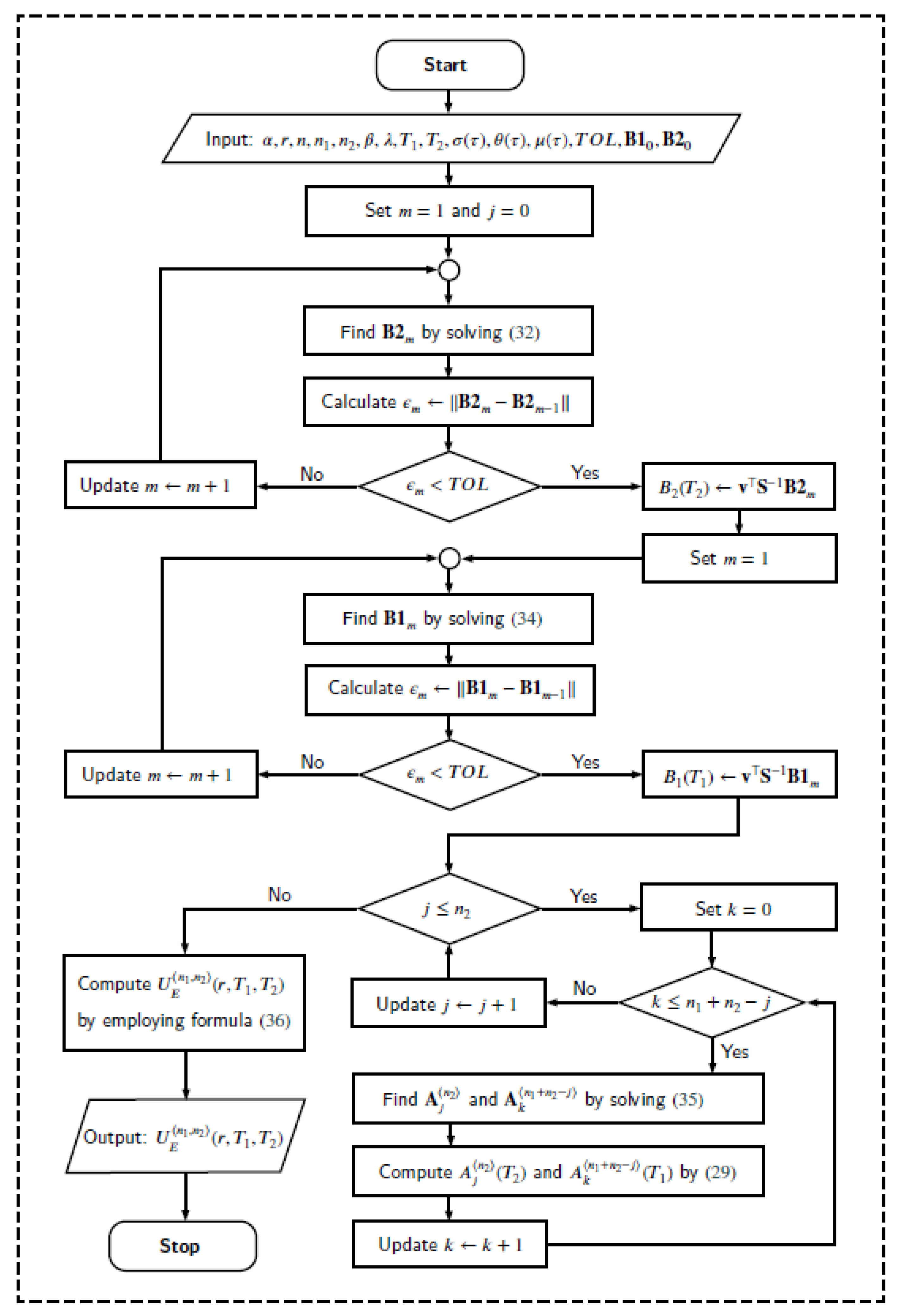
For computational convenience, we provide the algorithm for approximating the numerical formula of Theorem 4 in form of the flowchart, as demonstrated in Figure 2.

4.4. Numerical Validation

In this section, the validation testing of the obtained formulas in Section 3 is given through comparison with the MC simulations based on the ECIR(d) process proposed by Egorov et al. [21], the transition PDF of which is a consequence studied by Maghsoodi [5], i.e.,
d r t = θ σ 0 2 d e 2 σ 1 t 4 κ r t d t + σ 0 e σ 1 t r t d W t .
This process is recalled from Section 2. To compare the processes between (37) and (2), we have θ t = θ , μ t = d σ 2 t 4 θ and σ t = σ 0 e σ 1 t , where θ , σ 0 and σ 1 are constant real numbers and d N such that d 2 . These parameters make the functions θ ( t ) , μ ( t ) and σ ( t ) satisfy the Assumption 1. Moreover, the process (37) also has the transition PDF provided in Section 2, which may be usable to validate the value of U E γ ( r , τ ) .
However, this transition density is not a suitable validation for a small τ because it behaves like the Dirac delta function which has an infinitely thin spike when τ 0 , see [21]. As a result, it also produces an inaccurate solution U E γ ( r , τ ) . Therefore, for examining our formulas, we choose to employ the MC simulation to approximate them instead.
In these experiments, we also apply the technique of Euler–Maruyama (EM) discretization combined with the MC simulations to the process (37). This numerical scheme has been used to solve the ECIR process provided by Higham and Mao [28]. By EM method, we let r ^ be a time-discretized approximation of r and discretize the time interval [ 0 , T ] into N steps that are 0 = t 0 < t 1 < t 2 < < t N = T . Thus, the EM approximate is defined by:
r ^ t i + 1 = r ^ t i + θ ( t i ) μ ( t i ) r ^ t i Δ t + σ ( t i ) r ^ t i Δ t Z i + 1
with the initial value r ^ t 0 = r t 0 , where Δ t = t i + 1 t i is the time step and Z i is a standard normal random variable. Next, we illustrate the validations of the formulas via two examples under the CIR and ECIR processes. According to (37), we select the parameters d = 2 , θ = 1 , σ 0 = 0.01 and σ 1 = 0 , 1 that hold for Assumption 1. In addition, we can see that if σ 1 = 0 and σ 1 = 1 , the process (37) becomes the CIR and ECIR processes, respectively, as shown in Examples 1 and 2.
Our MC simulations are based on the EM method, implemented by the basic packages in MATLAB, to obtain numerical solutions of the SDE (37) to calculate (1) by using the Trapezoid integration method in the integral term. In all our calculations, MATLAB R2019a and a PC with the following details were utilized: Intel(R) Core(TM) i7-5700HQ, CPU @2.70GHz, 16.0GB (14.4 usable) RAM, Windows 8, 64-bit Operating System.
Example 1
(CIR case with σ 1 = 0 ). Use (11) in Theorem 3 under α = 0.01 , β = 0.02 and λ = 0.03 for n = 1 , 2 .
For n = 1 , we yield
U C 1 ( r , τ ) = e r B ( τ ) j = 0 1 A j 1 ( τ ) r 1 j = e r B ( τ ) A 0 1 ( τ ) r + A 1 1 ( τ )
and for n = 2 , we obtain
U C 2 ( r , τ ) = e r B ( τ ) j = 0 2 A j 2 ( τ ) r 2 j = e r B ( τ ) A 0 2 ( τ ) r 2 + A 1 2 ( τ ) r + A 2 2 ( τ )
for all r > 0 and τ = T t 0 , where the coefficients A j n ( τ ) and the solution B ( τ ) are given in Theorem 3. This example illustrates the formula based on the process (37) with σ 1 = 0 in the case of n N which actually gets the closed-form formula (11). Thus, validating the obtained closed-form formulas (39) and (40) under selecting the parameters d = 2 , θ = 1 , σ 0 = 0.01 and σ 1 = 0 for the process (37) with the MC simulations is shown in Figure 3. This implementation with MC method is simulated at each initial value r = 0.1 , 0.2 , 0.3 , , 1.6 to generate 10,000 sample paths of r t , where each path consists of 10,000 steps over the time lengths τ = 0.01 , 0.1 , 1 , 2 .
As displayed in Figure 3a, the results from MC simulations (circles) match completely with our formula (39) (solid lines) at every values r for n = 1 . Similarly, the results from the MC simulations in Figure 3b also attach with the results obtained from (40). However, the essential disadvantage of MC simulation is that it consumes expensive computational time for approximating the value at each initial value of r. In contrast, our closed-form formulas produce the exact solution for all initial values r > 0 and also give a shorter time in computation.
Example 2
(ECIR case with σ 1 = 1 ). Use (10) in Theorem 2 under α = 0.01 , β = 0.02 and λ = 0.03 for n = 1 , 2 .
For n = 1 , we yield
U E 1 ( r , τ ) e r B ( τ ) j = 0 1 A j 1 ( τ ) r 1 j = e r B ( τ ) A 0 1 ( τ ) r + A 1 1 ( τ )
and for γ = 2 to obtain
U E 2 ( r , τ ) e r B ( τ ) j = 0 2 A j 2 ( τ ) r 2 j = e r B ( τ ) A 0 2 ( τ ) r 2 + A 1 2 ( τ ) r + A 2 2 ( τ )
for all r > 0 and τ = T t 0 , where the coefficients A j n ( τ ) and the solution B ( τ ) are provided in Theorem 1. In this example, we test the validation by using the parameters d = 2 , θ = 1 , σ 0 = 0.01 and σ 1 = 1 . We see that these parameters produce the function σ ( t ) = 0.01 e t for which the Riccati differential equation cannot be solved analytically. Thus, the numerical method needs to be applied that has created in Section 4, the FIM with shifted Chebyshev polynomial, to approximate the coefficients A j n ( τ ) and B ( τ ) for calculating the formulas (41) and (42). In order to measure the accuracy of the obtained approximate results (41) and (42) by comparison with the MC simulations, we use the mean absolute error defined by:
E n ( τ ) : = i = 1 M U E n ( r i , τ ) W E n ( r i , τ ) ,
where U E n and W E n are, respectively, the approximate solutions obtained from the FIM and MC methods, r i is the i th initial value and M is the number of initial values used to test. Hence, the comparisons of numerical results of the formulas (41) and (42) with the MC simulations measured by the above mean absolute errors are demonstrated in Table 1 using initial values r = 0.1 , 0.2 , 0.3 , , 1.6 . For MC simulations, we vary the sample paths by 10,000, 20,000, 40,000 and 80,000 and each path is discretized into 10,000 steps. Table 1 shows that our approximate formulas for both n = 1 , 2 quite match with the results of MC simulations. Especially, for a small length of time τ such as τ = 0.01 in Table 1, they are very close to each other. Moreover, we also observe that they are more coincide as the number of sample paths increases. Consequently, the MC simulations are most likely converge to our approximate formulas. This confirms that our proposed numerical scheme for approximating the formulas in Example 2 is very accurate. Although our method and the MC simulation obtain the results most closely, the average run time (ART) to find their results at each initial r for both is very different. The ARTs consumption for our method is relatively inexpensive, i.e., less than a second. In contrast, the MC simulation consumes tremendous computational times, especially with large path numbers, which can be seen in Table 1.

5. Interest Rate Swap Pricing

A fixed-to-floating interest rate swap is an agreement for two parties to exchange a series of cash flows where a buyer agrees to pay a floating interest rate to receive a fixed interest rate on a predetermined principle, called a notional principle, over a specified period of time [8]; see Figure 4. It has many potential uses such as in risk management, portfolio management, and speculation. For instance, a company borrowing 10 million dollars from a bank with an interest rate of 3% plus the London Interbank Offered Rate (LIBOR) can sell a fixed-to-floating interest rate swap to hedge against the exposure to fluctuations in interest rates. Because the company will be paying a fixed interest rate instead of LIBOR, it will be much easier for the company to come up with a plan to allocate enough capital in order to service the debt. An interest rate swap is the most traded over-the-counter (OTC) swap at present. According to the Bank for International Settlements report on OTC interest rate derivatives in 2019 [29], the outstanding notional amount for the interest rate swap is over 300 trillion dollars.
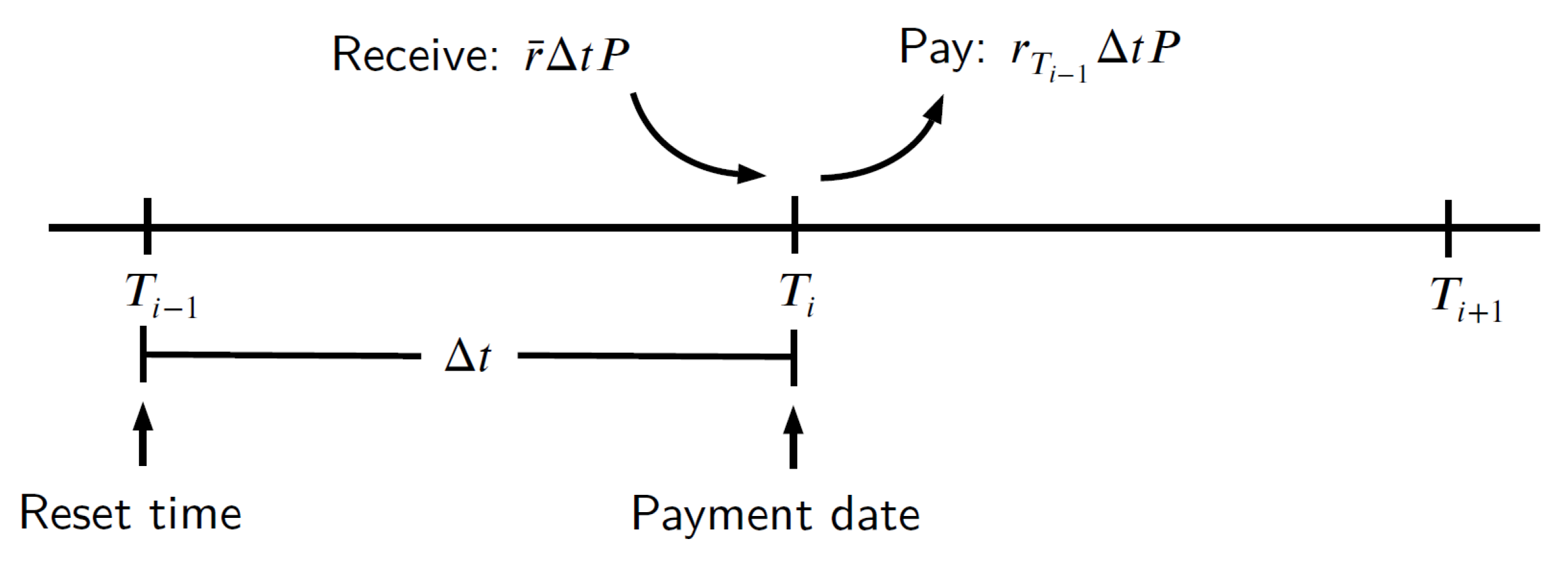
We consider two types of interest rate swaps, namely the arrears swap and the vanilla swap. The difference between the two swaps is the time which the floating interest rate is fixed at the reset time. A floating payment for an arrears swap is based on an interest rate at a payment time, whereas for a vanilla swap, the interest rate used to calculate the floating payment is fixed at the time before the payment time, which is usually the time of the previous payment. Thus, for an arrears swap, the payment date and the reset time coincide. The formulas for these swaps under the CIR process were proposed by Mallier and Alobaidi [8] using the Green’s function approach. Only the formula for the arrears swap is in a closed form. However, the formula is too complicated as it depends on the Kummer’s and gamma functions. In addition, the closed-form formula for the vanilla swap has not been derived. To the best of our knowledge, analytical formulas for both swaps under the ECIR process have not been discovered in any literature yet. This section provides analytical formulas for pricing such swaps under the ECIR process from the perspective of a buyer, i.e., a person who pays a floating interest rate to receive a fixed one. Under the CIR process, a special case of the ECIR process, such formulas are explicit.

5.1. Arrears Swaps

As interest rate swaps are OTC products, they can be customized differently to suit a buyer’s needs. We consider an interest rate swap contract such that fixed interest rate and floating interest rate payments are exchanged at every specified period of time, such as every three or six months over a predetermined time horizon such as two or ten years. At each payment date, an arrears swap buyer pays an interest on a notional principle determined by a floating interest rate at the time of the payment and receives a fixed interest. In other words, the reset time coincides with payment date.
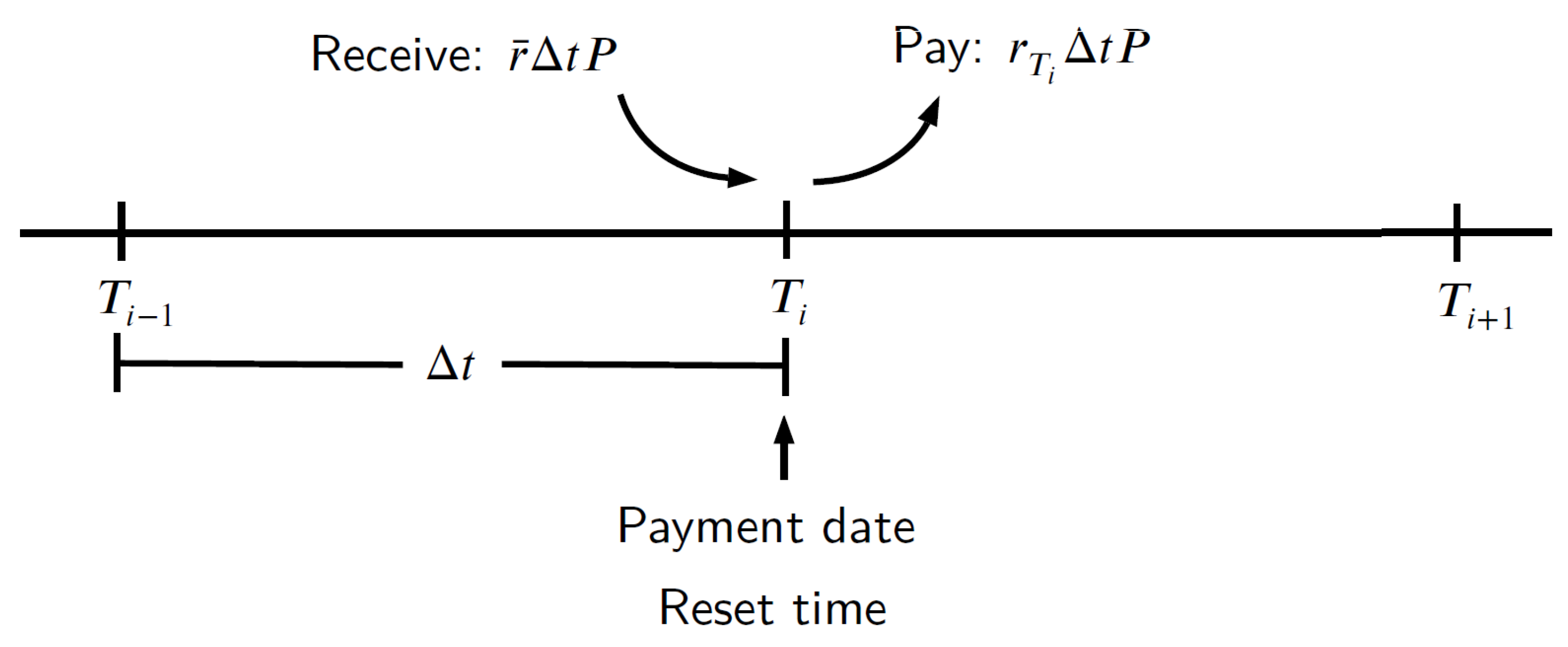
Let P denotes a notional principle, r ¯ denotes a fixed rate, and r t denotes a floating rate at time t. Assuming that an arrears swap has a maturity T and N payment dates at T 1 , T 2 , T 3 , , T N = T in an increment of Δ t , the payoff of such swap from a buyer’s point of view at the i th payment date, V i a r , which is just the difference between the interest on a notional principle determined by the fixed interest rate and the floating interest rate; see Figure 5, can be expressed by V i a r = ( r ¯ r T i ) Δ t P . By the fundamental theorem of asset pricing [6], the no-arbitrage price for the arrears swap is the expectation of the sum of each payoff discounted to time t under the risk neutral measure. Mathematically, the no-arbitrage price for the arrears swap, V ar , with an affine short rate discount, α r t + β where α , β R , can be expressed as:
V E a r : = E Q i = 1 N V i a r e t T i ( α r s + β ) d s r t = r .
By using Theorem 2, Theorem 5 shows an analytical formula for pricing an arrears swap. Under the CIR process, where all modeling parameters are constants, the pricing formula for the swap, derived in Corollary 3, becomes explicit.
Theorem 5.
Suppose that r t follows the ECIR process (2) with principle P > 0 and α, λ, β R . Let 0 t = T 0 < T 1 < T 2 < < T N = T . Then,
V E a r = Δ t P r ¯ i = 1 N U E 0 r , τ i i = 1 N U E 1 ( r , τ i )
for all r , τ i ( 0 , ) 2 , where τ i = T i t and Δ t = T i T i 1 for i = 1 , 2 , 3 , , N .
Proof. 
The arrears swap price formula follows (43) with V i a r = ( r ¯ r T i ) Δ t P and then
V E a r = E Q i = 1 N V i a r e t T i ( α r s + β ) d s r t = r = Δ t P r ¯ i = 1 N E Q e t T i ( α r s + β ) d s r t = r i = 1 N E Q r T i e t T i ( α r s + β ) d s r t = r .
Applying Theorem 2 with n = 0 and n = 1 yields (44). □
Corollary 3.
Suppose that r t follows the CIR process (2) with θ ( t ) = θ , μ ( t ) = μ and σ ( t ) = σ . According to Theorem 5, we have
V C a r = Δ t P i = 1 N exp 2 α ( e ρ τ i 1 ) r ρ e ρ τ i + 1 + θ e ρ τ i 1 β τ i 2 ρ e θ + ρ 2 τ i ρ e ρ τ i + 1 + θ e ρ τ i 1 2 θ μ σ 2 r ¯ 4 ρ 2 e ρ τ i r ρ e ρ τ + 1 + θ e ρ τ 1 2 2 θ μ e ρ τ i 1 ρ e ρ τ + 1 + θ e ρ τ 1 .
Proof. 
From the result in Theorem 5, we have
Δ t P r ¯ i = 1 N U C 0 ( r , τ i ) i = 1 N U C 1 ( r , τ i ) = Δ t P i = 1 N e B τ i r A 0 0 ( τ i ) r ¯ A 0 1 ( τ i ) r A 1 1 ( τ i ) ,
where the coefficients A 0 0 , A 0 1 and A 1 1 are given in Theorem 3. With some algebraic manipulations, it can be easily checked that the right-hand-side of (46) is equal to the left-hand-side of (45). □

5.2. Vanilla Swap

In contrast with an arrears swap, the interest rate determining the floating payment is set prior to the payment date, usually at the time of the previous payment. The cash flow of the vanilla swap is shown in Figure 6.
For a vanilla swap buyer, the payoff at the i th payment date is V i v a = ( r ¯ r T i 1 ) Δ t P . Similar to that of the arrears swap, the no-arbitrage price for a vanilla swap is
V E v a = E Q i = 1 N V i v a e t T i ( α r s + β ) d s r t = r .
In Theorem 6, we construct an analytical formula for pricing a vanilla swap by using Theorems 2 and 4. Corollary 4 shows that the formula is explicit under the CIR process.
Theorem 6.
Suppose that r t follows the ECIR process (2) with principle P > 0 and α, λ, β R . Let 0 t = T 0 < T 1 < T 2 < < T N = T . Then,
V E v a = Δ t P r ¯ i = 1 N U E 0 , 0 r , τ i 1 , Δ t r U E 0 , 0 r , 0 , Δ t i = 2 N U E 1 , 0 r , τ i 1 , Δ t ,
for all r , τ i 1 , Δ t ( 0 , ) 3 , where τ i = T i t and Δ t = T i T i 1 for i = 1 , 2 , 3 , , N .
Proof. 
The vanilla swap price formula follows (47) with V i a r = ( r ¯ r T i 1 ) Δ t P and then
V E v a = E Q i = 1 N V i v a e t T i ( α r s + β ) d s r t = r , = Δ t P r ¯ i = 1 N E Q e t T i ( α r s + β ) d s r t = r r E Q e t T 1 ( α r s + β ) d s r t = r i = 2 N E Q r T i 1 e t T i ( α r s + β ) d s r t = r .
Applying Theorem 4 to each term of the above conditional expectation; the first and second terms with n 1 = n 2 = 0 and the third term n 1 = 1 , n 2 = 0 , yields (48). □
Corollary 4.
Suppose that r t follows the CIR process (2) with θ ( t ) = θ , μ ( t ) = μ and σ ( t ) = σ . According to Theorem 6, we have
V C v a = Δ t P S 3 r ¯ r e r S 1 + i = 2 N e r S 2 r ¯ A 0 0 ( τ i 1 ; S 2 ) r A 0 1 ( τ i 1 ; S 2 ) A 1 1 ( τ i 1 ; S 2 ) ,
where ρ = θ 2 + 2 α σ 2 ,
S 1 : = B ( Δ t ; 0 ) = 2 α e ρ Δ t 1 ρ e ρ Δ t + 1 + θ e ρ Δ t 1 , S 2 : = B ( τ i 1 ; S 1 ) = S 1 ρ e ρ τ i 1 + 1 ( 2 α + S 1 θ ) e ρ τ i 1 1 ρ e ρ τ i 1 + 1 + θ S 1 σ 2 e ρ τ i 1 1 , S 3 : = A 0 0 ( Δ t ; S 1 ) = 2 ρ ρ e ρ Δ t + 1 + θ e ρ Δ t 1 2 θ μ σ 2 e β σ 2 + θ 2 μ + θ μ ρ σ 2 Δ t , A 0 0 ( τ i 1 ; S 2 ) = 2 ρ ρ e ρ τ i 1 + 1 + ( θ S 1 σ 2 ) e ρ τ i 1 1 2 θ μ σ 2 e β σ 2 + θ 2 μ + θ μ ρ σ 2 τ i 1 , A 0 1 ( τ i 1 ; S 2 ) = 2 ρ ρ e ρ τ i 1 + 1 + θ S 1 σ 2 e ρ τ i 1 1 2 θ μ σ 2 + 2 e σ 2 ( ρ β ) + θ 2 μ + θ μ ρ σ 2 τ i 1 and A 1 1 ( τ i 1 ; S 2 ) = θ μ e ρ τ i 1 1 ρ 2 ρ ρ e ρ τ i 1 + 1 + θ S 1 σ 2 e ρ τ i 1 1 2 θ μ σ 2 + 1 e β σ 2 + θ 2 μ + θ μ ρ σ 2 τ i 1 .
Proof. 
Obviously obtained from Theorem 6 and the parameter functions are given in Theorem 3. □
Clearly, our formulas for pricing IRSs are simpler and easier to use in practice compared with those in the literature. Under the CIR process, unlike the formulas by Mallier and Alobaidi’ [8], which consist of infinite integrals, which are not necessarily integrable, and Kummer’s function, our formulas are explicit. Under the ECIR process, these are the first analytical formulas for arrears and vanilla swaps pricing.

5.3. Examples

In this subsection, we compute the prices of both arrears and vanilla options under the modified ECIR(d) process which is to multiply the diffusion term of the ECIR(d) process proposed by Egorov et al. [21] with a parameter λ , i.e.,
d r t = θ σ 0 2 d e 2 σ 1 t 4 κ r t d t + λ σ 0 e σ 1 t r t d W t .
Note that if λ = 1 , the modified ECIR(d) process (50) becomes the original ECIR(d) process. The purpose of multiplying λ is to change the magnitude of the volatility without affecting the mean of the process. The parameter values used in this example are α = 1 , β = 0 , d = 5 , θ = 0.5 , σ = 0.15 and σ 1 = 0.001 . The modeling parameters values are taken from Table 1 of Egorov et al. [21].
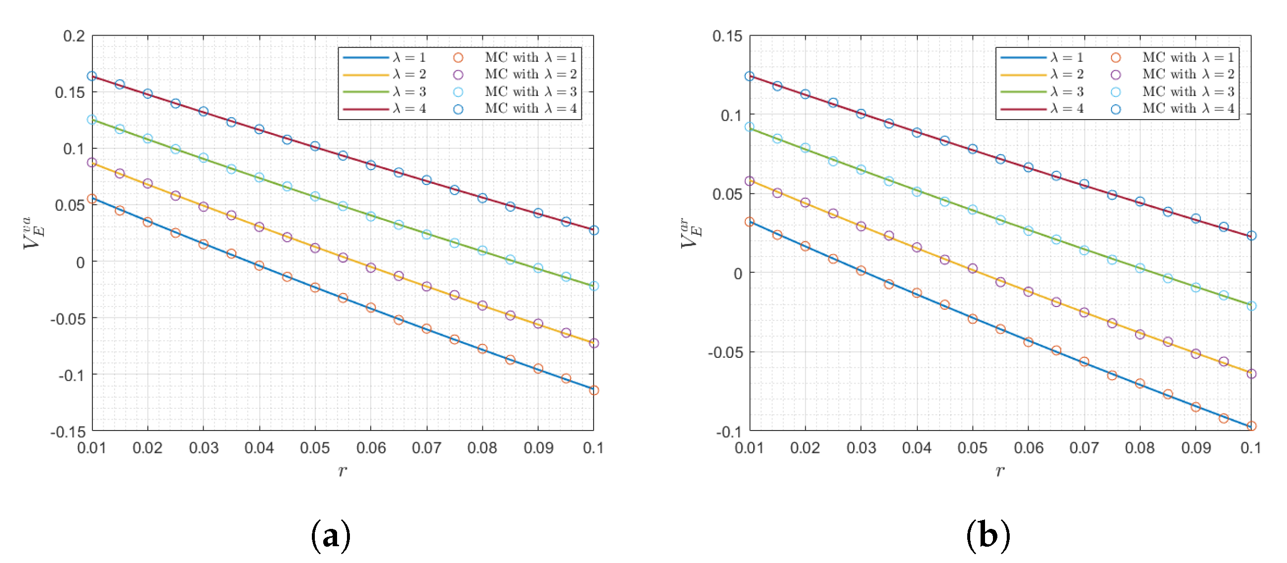
Figure 7 shows the prices of the arrears and vanilla swaps with 10-year maturity paid semi-annually computed using the formulas provided in Section 5 as functions of initial interest rates r for λ = 1 , 2 , 3 , 4 where the notional principle P = 1 and the fixed rate r ¯ = 0.05 .
The prices are compared with those obtained with MC simulations with 10,000 sample paths where each path has 10,000 steps. We see that the results most likely agree. However, as mentioned before, the MC simulation is computationally expensive. For each point, MC uses 600 s on average, whereas the scheme proposed in Section 5 consumes less than 0.001 s.
As mentioned above, the parameter λ describes the process’volatility. This means if the value of λ increases, the volatility of the process also increases. In practice, the higher the volatility, the more expensive the price. This agrees with the results shown in Figure 7a,b in which the parameters λ are varied from 1 to 4.

6. Fractional ECIR Process

This paper also considers the fractional ECIR process which is a class of fractional Pearson diffusions [30,31] where the first derivative with respect to time variable in (7) is replaced by a Caputo fractional derivative [32] of the order α ( 0 , 1 ) . In real-world applications, time-fractional diffusion equations are useful in many branches of science, especially in finance. For instance, the time-fractional diffusion is used to model the delays between trades based on the continuous-time random walks, and they have been applied to extend the Black–Scholes formula in a subdiffusive regime [33,34].
Before embarking into the details of fractional ECIR process, we provide the basic definitions of fractional derivatives. The necessary notations and some important facts used throughout this section are also given. More details on definitions and basic results of fractional calculus can be found in [35].
Definition 2
([36]). The Caputo fractional derivative of order α ( 0 , 1 ) is defined by
α u ( r , τ ) τ α = 1 Γ ( 1 α ) 0 τ u ( r , s ) s ( τ s ) α d s ,
where u is differentiable in τ (or even absolutely continuous).
For fractional order α ( 0 , 1 ) , we consider a fractional backward equation that corresponds to the ECIR process (2), it can be expressed in the form of the fractional Cauchy problem (presented by Leonenko et al. in [30]), that is
α u τ α = θ ( T τ ) μ ( T τ ) r u r + r σ 2 ( T τ ) 2 2 u r 2 ,
subject to the initial condition u ( r , 0 ) = g ( r ) . Moreover, we have known that a solution of this problem provided in [30] that is in the expectation form, i.e.,
u ( r , t ) = E α Q g r T r t = r .
By applying the solution of the fractional Cauchy problem (52) with the same technique proposed in Section 3, it can be extendable to solve a certain of time-fractional diffusion problem. For instance, a time-fractional conditional moment which can be expressed by:
E α Q r T n r t = r = j = 0 n A j ( τ ) r n j : = u α n ( r , τ ) ,
where the coefficient functions A j ( τ ) satisfy:
α A 0 ( τ ) τ α = θ n A 0 ( τ ) ,
α A j ( τ ) τ α = θ ( n j ) A j ( τ ) + n j + 1 θ μ ( n j ) σ 2 2 A j 1 ( τ ) ,
for all j = 1 , 2 , 3 , , n , where θ : = θ ( T τ ) , μ : = μ ( T τ ) and σ : = σ ( T τ ) .
The motivation for the form (54) of the solution to fractional differential Equation (52) is based on the results of [37,38]. Since the fractional Pearson diffusions has linear drift and quadratic squared diffusion coefficient, the differential generator (52) maps polynomials to polynomials (see more details in [37,38]). Roughly speaking, using (52) with u : = u α n ( r , τ ) for all ( r , τ ) ( 0 , ) × [ 0 , ) , subject to the initial condition:
j = 0 n A j ( 0 ) r n j = u α γ ( r , 0 ) = E α Q r T n r T = r = r n .
By comparing the coefficients in r, we obtain the conditions A 0 ( 0 ) = 1 and A j ( 0 ) = 0 for all j = 0 , 1 , 2 , , n . Computing (52) using (54), we have:
1 Γ ( 1 α ) 0 τ j = 0 n A j ( s ) r n j ( τ s ) α d s = θ n A 0 ( τ ) r n + j = 1 n θ ( n j ) A j ( τ ) + n j + 1 θ μ ( n j ) σ 2 2 A j 1 ( τ ) r n j ,
and we also have
1 Γ ( 1 α ) 0 τ A 0 ( s ) r n ( τ s ) α d s + 1 Γ ( 1 α ) 0 τ j = 1 n A j ( s ) r n j ( τ s ) α d s = θ n A 0 ( τ ) r n + j = 1 n θ ( n j ) A j ( τ ) + n j + 1 θ μ ( n j ) σ 2 2 A j 1 ( τ ) r n j .
Therefore, by comparing the coefficients in r, the above equation can be solved through a system of time-fractional differential Equations (55) and (56). Thus, the coefficient parameters A j ( τ ) can be calculated from (55) and (56). However, the solutions of (55) and (56) are always unavailable in closed form. Thus, a numerical method is needed.
Next, to find the coefficient functions A j ( τ ) , we investigate a numerical scheme to solve the time-fractional differential equations (55) and (56). Let us first uniformly discretize the time domain [ 0 , τ ] into m steps, i.e., τ i = i Δ τ for i = 0 , 1 , 2 , , m , where Δ t is a time step. Then, we have:
α A 0 ( τ ) τ α | τ = τ m = θ m n A 0 m ,
α A j ( τ ) τ α | τ = τ m = θ m ( n j ) A j m + n j + 1 θ m μ m ( n j ) ( σ m ) 2 2 A j 1 m ,
where A j m : = A j ( τ m ) , θ m : = θ ( T τ m ) , μ m : = μ ( T τ m ) and σ m : = σ ( T τ m ) . Then, we consider the time-fractional derivative terms of (58) and (59) by employing the Caputo fractional derivative in Definition 2. We obtain:
α A j ( τ ) τ α | τ = τ m = 1 Γ ( 1 α ) 0 τ m A j ( s ) ( τ m s ) α d s = 1 Γ ( 1 α ) i = 0 m 1 τ i τ i + 1 A j ( s ) ( τ m s ) α d s .
After that, we use the first-order forward difference quotient to approximate the time derivative term in the above equation. For convenience, we also adjust the index in the last step of the following process by defining k : = m i 1 . Then,
α A j ( τ ) τ α | τ = τ m 1 Γ ( 1 α ) i = 0 m 1 1 Δ τ A j i + 1 A j i τ i τ i + 1 ( τ m s ) α d s = ( Δ τ ) 1 Γ ( 1 α ) i = 0 m 1 A j i + 1 A j i ( τ m τ i ) 1 α ( τ m τ i + 1 ) 1 α 1 α = ( Δ τ ) α Γ ( 2 α ) i = 0 m 1 A j i + 1 A j i ( m i ) 1 α ( m i 1 ) 1 α = ( Δ τ ) α Γ ( 2 α ) k = 0 m 1 A j m k A j m k 1 ( k + 1 ) 1 α k 1 α = k = 1 m 1 w k α A j m k A j m k 1 + w 0 α A j m w 0 α A j m 1 ,
where w k α = ( Δ t ) α Γ ( 2 α ) ( k + 1 ) 1 α k 1 α . Now, we can replace (60) into (58) and (59) which rearrange to obtain the explicit coefficient functions A j m as follows
A 0 m = 1 w 0 α + θ m n w 0 α A 0 m 1 k = 1 m 1 w k α A 0 m k A 0 m k 1 , A j m = 1 w 0 α + θ m ( n j ) w 0 α A j m 1 k = 1 m 1 w k α A j m k A j m k 1
+ n j + 1 w 0 α + θ m ( n j ) θ m μ m ( n j ) ( σ m ) 2 2 A j 1 m .
Note that for m = 1 , the summation term is set to be zero. Therefore, the solutions of A j ( τ m ) can be approximated by running the iterative system (61) and (62), respectively, staring with A 0 0 = 1 and A j 0 = 0 for j = 1 , 2 , 3 , , n . Finally, we can also obtain a numerical result of the time-fractional conditional moment (54) that is:
E α Q r T n r t = r = u α n ( r , τ m ) j = 0 n A j m r n j .
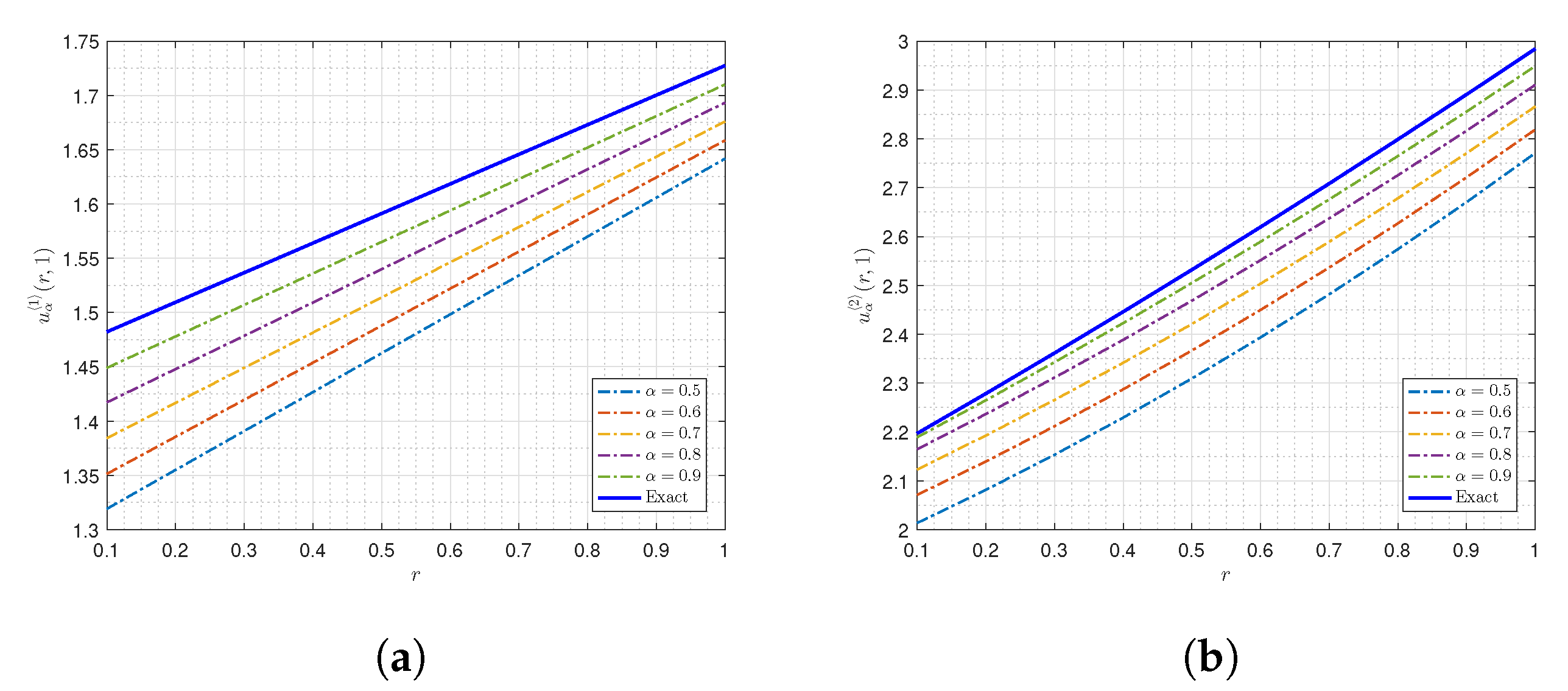
Next, to test the efficiency of our proposed numerical scheme, we examine by varying the fractional order α ( 0 , 1 ) of Examples 3 and 4 for both first- and second-moment of conditional expectations with the following parameters θ = 1.3 , μ = 2 and σ = 0.1 at the terminal time T = 1 .
Example 3.
The 1st-moment of fractional ECIR: E α Q r T r t = r = u α 1 ( r , 1 ) with α ( 0 , 1 ) .
Example 4.
The 2nd-moment of fractional ECIR: E α Q r T 2 r t = r = u α 2 ( r , 1 ) with α ( 0 , 1 ) .
By using the proposed numerical scheme described in this section, we examine the behavior of the solutions (54) for various values of α ( 0 , 1 ) by discretizing the time domain [ 0 , 1 ] into 100 steps distributed uniformly. Then, we can demonstrate the plotting solutions u α 1 ( r , 1 ) and u α 2 ( r , 1 ) for r ( 0 , 1 ] of both examples by varying the fractional order α { 0.5 , 0.6 , , 0.7 , 0.8 , 0.9 } . We can obviously see that when α 1 , the behavior of the obtained approximate solutions, depicted in Figure 8, tends to the blue solid line, i.e., the integer order solution at α = 1 obtained by Formula (11) with parameters λ = α = β = 0 .
Remark 4.
The idea presented in this section can be also applied to the generalised geometric Brownian motion (GBM), which the standard and subdiffusive GBM arise as special cases, see [39] for more details.

7. Conclusions and Discussions

In this paper, we first study the conditional expectation of the product of polynomial and exponential functions, E Q r T γ e λ r T t T ( α r s + β ) d s r t = r where α , λ , β , γ R and r t follows ECIR process. By solving the PDE (7) derived from the Feynman–Kac representation, we archive an analytical formula of the conditional expectation given in (1) for the ECIR process in terms of the infinite sum of analytical expressions as shown in Theorem 1. Interestingly, the infinite sum can be reduced to a finite sum if γ N { 0 } , as shown in Theorem 2. We also show that under the CIR process, which is a special case of the ECIR process, as the parameters given in (4) can be integrable. The Riccati differential Equation (5) can be solved analytically. The formula of the expectation can be expressed in the closed form as in Theorem 3. The formula is then extended to derive the expectation of a product of two polynomials and exponential functions, E Q r s n 1 r T n 2 e t T ( α r u + β ) d u r t = r where n 1 , n 2 N { 0 } and 0 t < s < T , see Theorem 4.
In addition, in Section 4, we propose the numerical scheme constructed using the FIM with shifted Chebyshev polynomials to evaluate the expectation (1) when the Riccati differential equation cannot be solved analytically and show its efficiency as well as its accuracy by comparing it with the MC simulations.
To illustrate an application of such formulas in finance, we apply the Formula (10) in Theorem 2 and the formula (17) in Theorem 4 to derive the analytical pricing formulas for two interest rate swaps, namely the arrears swap and vanilla swaps under the ECIR process. It is shown that the formulas for such swaps are explicit under the CIR process. The numerical pricing examples for both swaps under the ECIR process are also given. Finally, in Section 6, we provide a study case of the fractional ECIR process and adopt the idea from our main results.

Author Contributions

Conceptualization, R.B., U.R., A.D. and P.S.; methodology, A.D. and P.S.; software, A.D. and P.S.; validation, R.B., U.R., A.D. and P.S.; formal analysis, R.B., U.R., A.D. and P.S.; investigation, R.B., U.R., A.D. and P.S.; writing—original draft preparation, A.D. and P.S.; writing—review and editing, R.B. and U.R.; visualization, A.D. and P.S.; supervision, R.B. and U.R.; project administration, U.R.; funding acquisition, R.B. All authors have read and agreed to the published version of the manuscript.

Funding

This research received no external funding.

Institutional Review Board Statement

Not applicable.

Informed Consent Statement

Not applicable.

Data Availability Statement

Not applicable.

Acknowledgments

We are grateful for a variety of valuable suggestions from the anonymous referees which have substantially improved the quality and presentation of the results. All errors are the author’s own responsibility. This research project is supported by Second Century Fund (C2F), Chulalongkorn University.

Conflicts of Interest

The authors declare no conflict of interest.

Abbreviations

The following abbreviations are used in this manuscript:
ARTaverage run time
CCAConvexity correction approximation
CIRCox–Ingersoll–Ross
EMEuler–Maruyama
ECIRExtended Cox–Ingersoll–Ross
FIMFinite integration method
FRAForward rate agreement
IRSInterest rate swap
LIBORLondon Interbank Offered Rate
MCMonte Carlo
OTCOver-the-counter
PDEPartial differential equation
PDFProbability density function
SDEStochastic differential equation

References

  1. Hull, J.; White, A. Pricing interest-rate-derivative securities. Rev. Financ. Stud. 1990, 3, 573–592. [Google Scholar] [CrossRef]
  2. Feller, W. Two singular diffusion problems. Ann. Math. 1951, 54, 173–182. [Google Scholar] [CrossRef]
  3. Cox, J.C.; Ingersoll, J.E., Jr.; Ross, S.A. An intertemporal general equilibrium model of asset prices. Econ. J. Econ. Soc. 1985, 53, 363–384. [Google Scholar] [CrossRef] [Green Version]
  4. Hansen, L.P.; Scheinkman, J.A. Back to the Future: Generating Moment Implications for Continuous-Time Markov Processes; National Bureau of Economic Research: New York, NY, USA; National Bureau of Economic Research: Cambridge, MA, USA, 1993. [Google Scholar]
  5. Maghsoodi, Y. Solution of the extended CIR term structure and bond option valuation. Math. Financ. 1996, 6, 89–109. [Google Scholar] [CrossRef]
  6. Delbaen, F.; Schachermayer, W. A general version of the fundamental theorem of asset pricing. Math. Ann. 1994, 300, 463–520. [Google Scholar] [CrossRef]
  7. Duffie, D.; Pan, J.; Singleton, K. Transform analysis and asset pricing for affine jump-diffusions. Econometrica 2000, 68, 1343–1376. [Google Scholar] [CrossRef] [Green Version]
  8. Mallier, R.; Alobaidi, G. Interest rate swaps under CIR. J. Comput. Appl. Math. 2004, 164, 543–554. [Google Scholar] [CrossRef] [Green Version]
  9. Moreno, M.; Platania, F. A cyclical square-root model for the term structure of interest rates. Eur. J. Oper. Res. 2015, 241, 109–121. [Google Scholar] [CrossRef]
  10. Frenkel, D.; Portugal, R. Algebraic methods to compute Mathieu functions. J. Phys. A Math. Gen. 2001, 34, 3541. [Google Scholar] [CrossRef]
  11. Thamrongrat, N.; Rujivan, S. An analytical formula for pricing interest rate swaps in terms of bond prices under the extended Cox–Ingersoll–Ross model. Songklanakarin J. Sci. Technol. 2020, 43, 987–992. [Google Scholar]
  12. Gouriéroux, C.; Valéry, P. Estimation of a Jacobi process. Preprint 2004, 116, 1–67. [Google Scholar]
  13. Dufresne, D. The Integrated Square-Root Process; Research Paper No. 90; University of Melbourne: Melbourne, Australia, 2001; pp. 1–34. [Google Scholar]
  14. Rujivan, S. A closed-form formula for the conditional moments of the extended CIR process. J. Comput. Appl. Math. 2016, 297, 75–84. [Google Scholar] [CrossRef]
  15. Sutthimat, P.; Mekchay, K.; Rujivan, S. Explicit Formula for Conditional Expectations of Product of Polynomial and Exponential Function of Affine Transform of Extended Cox–Ingersoll–Ross Process. J. Phys. Conf. Ser. 2018, 1132, 012083. [Google Scholar] [CrossRef]
  16. Grasselli, M. The 4/2 stochastic volatility model: A unified approach for the Heston and the 3/2 model. Math. Financ. 2017, 27, 1013–1034. [Google Scholar] [CrossRef]
  17. Boonklurb, R.; Duangpan, A.; Gugaew, P. Numerical solution of direct and inverse problems for time-dependent Volterra integro-differential equation using finite integration method with shifted Chebyshev polynomials. Symmetry 2020, 12, 497. [Google Scholar] [CrossRef] [Green Version]
  18. Duangpan, A.; Boonklurb, R.; Treeyaprasert, T. Finite Integration Method with Shifted Chebyshev Polynomials for Solving Time-Fractional Burgers’ Equations. Mathematics 2019, 7, 1201. [Google Scholar] [CrossRef] [Green Version]
  19. Chihara, T.S. An Introduction to Orthogonal Polynomials; Courier Corporation: Gordon and Breach: New York, NY, USA, 1978. [Google Scholar]
  20. Leonenko, G.M.; Phillips, T.N. High-order approximation of Pearson diffusion processes. J. Comput. Appl. Math. 2012, 236, 2853–2868. [Google Scholar] [CrossRef] [Green Version]
  21. Egorov, A.V.; Li, H.; Xu, Y. Maximum likelihood estimation of time-inhomogeneous diffusions. J. Econom. 2003, 114, 107–139. [Google Scholar] [CrossRef]
  22. Chumpong, K.; Mekchay, K.; Rujivan, S. A simple closed-form formula for the conditional moments of the Ornstein-Uhlenbeck process. Songklanakarin J. Sci. Technol. 2020, 42, 836–845. [Google Scholar]
  23. Kijima, M. Stochastic Processes with Applications to Finance; CRC Press: Boca Raton, FL, USA, 2016. [Google Scholar]
  24. Zhu, S.P.; Lian, G.H. On the convexity correction approximation in pricing volatility swaps and VIX futures. New Math. Nat. Comput. 2018, 14, 383–401. [Google Scholar] [CrossRef]
  25. Boonklurb, R.; Duangpan, A.; Treeyaprasert, T. Modified finite integration method using Chebyshev polynomial for solving linear differential equations. J. Numer. Ind. Appl. Math. 2018, 12, 1–19. [Google Scholar]
  26. Boyd, J.P. Chebyshev and Fourier Spectral Methods, 2nd ed.; DOVER Publications: Mineola, NY, USA, 2001. [Google Scholar]
  27. Caro-Lopera, F.J.; Leiva, V.; Balakrishnan, N. Connection between the Hadamard and matrix products with an application to matrix-variate Birnbaum-Saunders distributions. J. Multivar. Anal. 2012, 104, 126–139. [Google Scholar] [CrossRef] [Green Version]
  28. Higham, D.J.; Mao, X. Convergence of Monte Carlo simulations involving the mean-reverting square root process. J. Comput. Financ. 2005, 8, 35–61. [Google Scholar] [CrossRef] [Green Version]
  29. Saupe, S. The foreign exchange and over-the-counter interest rate derivatives market in Ireland–Results of the BIS Triennial Survey 2019. Quart. Bull. Articles 2020, 53, 106–124. [Google Scholar]
  30. Leonenko, N.N.; Meerschaert, M.M.; Sikorskii, A. Fractional Pearson diffusions. J. Math. Anal. Appl. 2013, 403, 532–546. [Google Scholar] [CrossRef] [PubMed]
  31. Sutthimat, P.; Mekchay, K. Closed-form formulas for conditional moments of inhomogeneous Pearson diffusion processes. Commun. Nonlinear Sci. Numer. Simul. 2022, 106, 106095. [Google Scholar] [CrossRef]
  32. Caputo, M. Linear models of dissipation whose Q is almost frequency independent—II. Geophys. J. Int. 1967, 13, 529–539. [Google Scholar] [CrossRef]
  33. Magdziarz, M. Black–Scholes formula in subdiffusive regime. J. Stat. Phys. 2009, 136, 553–564. [Google Scholar] [CrossRef]
  34. Stanislavsky, A. Black–Scholes model under subordination. Phys. A Stat. Mech. Its Appl. 2003, 318, 469–474. [Google Scholar] [CrossRef] [Green Version]
  35. Podlubny, I. Fractional Differential Equations; Academic Press: San Diego, CA, USA, 1998. [Google Scholar]
  36. Eidelman, S.D.; Ivasyshen, S.D.; Kochubei, A.N. Analytic Methods in the Theory of Differential and Pseudo-Differential Equations of Parabolic Type; Springer Science & Business Media: Berlin/Heidelberg, Germany, 2004; Volume 152. [Google Scholar]
  37. Forman, J.L.; Sørensen, M. The Pearson diffusions: A class of statistically tractable diffusion processes. Scand. J. Stat. 2008, 35, 438–465. [Google Scholar] [CrossRef]
  38. Schmidt, M.F. Pearson Diffusions with Jumps. Ph.D. Thesis, Technische Universitat Munchen, Munchen, Germany, 2008. [Google Scholar]
  39. Stojkoski, V.; Sandev, T.; Basnarkov, L.; Kocarev, L.; Metzler, R. Generalised geometric Brownian motion: Theory and applications to option pricing. Entropy 2020, 22, 1432. [Google Scholar] [CrossRef] [PubMed]
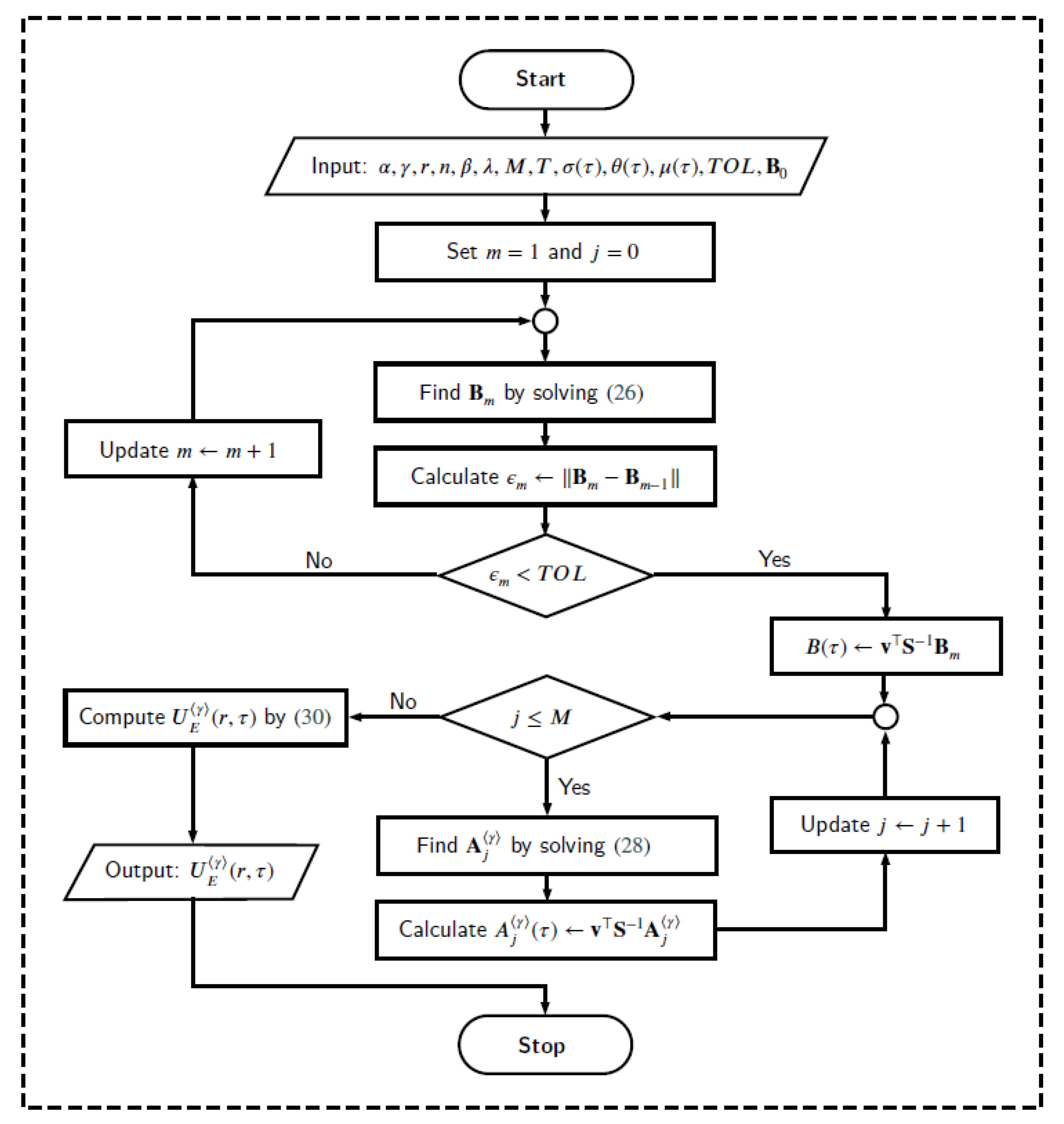
Figure 1. The flowchart for computing numerical formula of Theorem 1.
Fractalfract 06 00058 g001
Figure 2. The flowchart for computing numerical formula of Theorem 4.
Fractalfract 06 00058 g002
Figure 3. The validation testings of U C n ( r , τ ) for the initial rates r = 0.1 , 0.2 , 0.3 , , 1.6 and τ = 0.01 , 0.1 , 1 , 2 . (a) Conditional expectation U C 1 ( r , τ ) . (b) Conditional expectation U C 2 ( r , τ ) .
Fractalfract 06 00058 g003
Figure 4. Mechanic of a fix-to-floating interest rate swap.
Fractalfract 06 00058 g004
Figure 5. Cash flow of an arrears swap at time T i .
Fractalfract 06 00058 g005
Figure 6. Cash flow of a vanilla swap at time T i .
Fractalfract 06 00058 g006
Figure 7. Valuations of IRSs V E a r and V E v a as functions of initial interest rate with a fixed rate r ¯ = 0.05 and a notional principle P = 1 . (a) Arrears swaps V E a r . (b) Vanilla swaps V E v a .
Fractalfract 06 00058 g007
Figure 8. The behaviors of the approximate solutions u α 1 ( r , 1 ) and u α 2 ( r , 1 ) in Examples 3 and 4. (a) The 1st-moment u α 1 ( r , 1 ) . (b) The 2nd-moment u α 2 ( r , 1 ) .
Fractalfract 06 00058 g008
Table 1. The mean absolute error E n ( τ ) of U E n ( r , τ ) for for the initial rates r = 0.1 , 0.2 , 0.3 , , 1.6 and τ = 0.01 , 0.1 , 1 , 2 .
nNo. of PathsARTs (s) τ
0 . 01 0 . 1 1 2
110,00012.897.1050 × 10 6 2.0675 × 10 5 6.3625 × 10 5 1.5488 × 10 4
20,00026.564.5500 × 10 6 1.6513 × 10 5 4.1245 × 10 5 6.4814 × 10 5
40,00051.884.1990 × 10 6 9.9830 × 10 6 3.6479 × 10 5 5.3519 × 10 5
80,000110.75  2.9145 × 10 6 6.1815 × 10 6 3.3202 × 10 5 3.5518 × 10 5
210,00013.751.4354 × 10 5 6.9159 × 10 5 3.6182 × 10 5 2.3756 × 10 5
20,00026.016.6300 × 10 6 4.0234 × 10 5 2.6777 × 10 5 1.8003 × 10 5
40,00049.465.8490 × 10 6 2.3235 × 10 5 1.9620 × 10 5 1.6697 × 10 5
80,000111.13  3.7426 × 10 6 2.2077 × 10 5 1.4912 × 10 5 1.4263 × 10 5
Publisher’s Note: MDPI stays neutral with regard to jurisdictional claims in published maps and institutional affiliations.