A Fast L2-1_σ Finite Element Method for Time Fractional Keller–Segel Equations with Weakly Singular Solutions

Abstract

We propose a fast L2-1_σ finite element method for solving the time fractional Keller–Segel equations with a Caputo fractional derivative of $\alpha \in (0,1)$. Firstly, the fast L2-1_σ scheme on the graded mesh is used to discretize the time fractional derivative. This approach relies on the sum of exponentials (SOE) skill to speed up the convolution kernel. Thus, we overcome the computational cost caused by the nonlocality of fractional derivatives. Then, by combining finite element discretization in spatial direction, a fully implicit numerical scheme is derived. Subsequently, we establish the stability and an $\alpha$-robust error analysis of the fully discrete scheme. Finally, we present some numerical examples to demonstrate the correctness of our theoretical results.

1. Introduction

In recent years, fractional partial differential equations have been widely applied in different branches, for instance, biology [1], physics [2], control system [3], and finance [4]. And a large number of researchers have shown great interest in theoretical and numerical analysis. Let $\Omega$ be a open and bounded domain of ${\mathbb{R}}^d(d\ge 1)$ with a smooth boundary $\partial \Omega$. Given $\alpha \in (0,1)$, we shall be interested in the numerical approximation for a time-fractional Keller–Segel (TFKS) equation

$$\left\{\begin{array}{cc}{\partial }_t^{\alpha }u-\Delta u+\nabla ·(u\nabla v)=0,\hfill & x\in \Omega ,0<t<T,\hfill \\ {\partial }_t^{\alpha }v-\Delta v+v=u,\hfill & x\in \Omega ,0<t<T,\hfill \\ u(x,t)=v(x,t)=0,\hfill & x\in \partial \Omega ,0<t<T,\hfill \\ u(x,0)=u_0\left(x\right),v(x,0)=v_0\left(x\right),\hfill & x\in \Omega ,\hfill \end{array}\right.$$

(1)

where $u_0,v_0$ are a given functions, and ${\partial }_t^{\alpha }u$ represents the Caputo fractional derivative, which is defined as

$${\partial }_t^{\alpha }u\left(t\right)={\int }_0^t{w}_{1-\alpha }(t-\xi )u^{\prime }\left(\xi \right)d\xi ,\mathrm{with}{w}_{\alpha }={\displaystyle \frac{t^{\alpha -1}}{\Gamma \left(\alpha \right)}}.$$

(2)

When $\alpha =1$, model (1) is called the classic Keller–Segel (KS) equation, which was first introduced in [5,6] to capture the chemotaxis response of bacteria towards chemical agents, where $u(x,t)$ stands for the density of bacteria and $v(x,t)$ represents the concentration of the oxygen. In biology and mathematics, diffusion and chemotaxis are the basis of the motion of bacteria [7,8]. Thus, KS equations provide a powerful framework to understand the intricate interplay between the motion of bacteria, chemical signaling, and emergent pattern formation [9]. However, anomalous diffusion is a ubiquitous phenomenon in the process of biological movement [10,11,12]. Moreover, we note that anomalous diffusion can be modeled as continuous-time random walks at the macroscopic level [13], so we can modify the diffusion equation by applying a fractional temporal operator. For instance, Langlands and Henry [14] developed fractional chemotaxis diffusion equations with anomalous diffusion for modeling the chemically directed transport of biological organisms. Their work studied the influence of substrate heterogeneity on the dynamics of the KS model by the means of fractional calculus in [15].

Let us recall some work in the literature concerning TFKS equations with the Caputo fractional derivative. By the Aubin–Lions lemma and its variants, the existence of a weak solution was introduced in [16]. Zhou et al. [17] proved the existence of a solution by using the Faedo–Galerkin method with some compactness arguments, and the Mittag–Leffler stability of the solution was given. Their work has established the existence of the nonnegative weak solution in [18]. In [19], some refined results regarding the large time behavior of solutions were derived, and the well-posedness and the asymptotic stability of solutions in Marcinkiewicz spaces were studied. The well-posedness and the blow-up of the solution were established in the setting of Lebesgue and Besov spaces from [20]. El-Sayed et al. [21] obtained the analytical solution by the Adomians decomposition method. The modified homotopy analysis transform method was developed in [22]. Additionally, studies on the fractional KS equations with other fractional derivative operators can be found in [23,24,25,26].

Less work has been carried out on the numerical methods of the TFKS equation. To our knowledge, it is only mentioned in [27]. This work proposed a fractional class of explicit Adams–Bashforth and implicit Adams–Moulton methods of first-and second-order accuracy to solve the TFKS equations with the sufficiently smooth solution. Nevertheless, a growing number of studies suggest that the solution of the time fractional partial differential equations is weakly singular near $t=0$ [28,29], i.e., there exists a constant C, for any $t\in (0,T]$:

$$\left|{\partial }_t^{l}u\left(t\right)\right|\le C\left(1+t^{\alpha -l}\right),l\in \mathbb{N},$$

To overcome the initial time singularity, the L1, L2-1_σ, L2 and DG methods on the graded meshes or general nonuniform meshes have been developed in [30,31,32,33,34,35]. The L1, L2 and CQ schemes with proper initial correction using uniform step size can recover the optimal error estimates; see [36,37,38,39]. Another important feature is the problem of large computational cost due to the nonlocality of the fractional derivatives. Then, the fast L1, L2 and L2-1_σ schemes based on the sum of exponentials (SOE) approximation were proposed and analyzed in [40,41,42,43,44].

The main difficulties in the study of problem (1) are the weak singularity and nonlocality of the fractional time derivative and the nonlinearity of the equation itself. In order to derive high-precision numerical solutions, we firstly use the nonuniform L2-1_σ scheme to handle the singularity of solutions at the initial time, and this scheme is high-order. Inspired by [45,46], we shall adopt the SOE approximation to speed up the computation of the L2-1_σ scheme, thus reducing the computational storage and computational cost from $\mathcal{O}\left(N\right)$ and $\mathcal{O}\left(N^2\right)$ to $\mathcal{O}\left(N_{exp}\right)$ and $\mathcal{O}\left(N{N}_{exp}\right)$, respectively. Here N denotes the number of time step and $N_{exp}$ stands for the number of the quadrature nodes. Next, we use the finite element to discretize spatial direction and combine it with the fast L2-1_σ method to obtain an implicit scheme. Compared to the explicit scheme, our approach is unconditionally stable, and its accuracy will not decrease. By the improved fractional Grönwall inequality, we further prove the stability and the $\alpha$-robust error estimates of the numerical scheme. Finally, some numerical results demonstrate the correctness of the theoretical analysis.

The main contributions of our work are as follows:

• We consider for the first time the numerical method for solving singular cases in the fractional KS models. Compared to the smooth case in reference [27], our numerical method is more in line with the characteristics of fractional order models.
• A fast numerical scheme is obtained by constructing a fast nonuniform L2-1_σ scheme with the finite element method for the time fractional Keller–Segel equations. This numerical scheme has the advantages of high accuracy and low computational storage and can effectively handle the singularity of the solution at $t\to 0$.
• We prove the stability of the numerical scheme for both the $L^2(\Omega )$ and $H^1(\Omega )$ norms under some constraints on the time step ratio and obtain a $\alpha$-robust error estimate by the fractional Grönwall inequality. We note that this theoretical analysis framework is also applicable to the more complex time fractional-order coupled diffusion systems [47].

The outline of this work is as follows. In Section 2, a fast L2-1_σ method and the fully discrete scheme are introduced. In Section 3, we establish the unconditional stability of the fully discrete scheme in both $L^2(\Omega )$ and $H^1(\Omega )$ norms. In Section 4, an $\alpha$-robust error estimate is provided in both $L^2(\Omega )$ and $H^1(\Omega )$ norms. In Section 5, we propose several numerical examples to verify theoretical analysis. Finally, a summary of this work is made in Section 6.

2. Fully Discrete Scheme for the TFKS Equations

Let $L^p(\Omega )$ be the Lebesgue space with norm ${\parallel ·\parallel }_{0,p}$ for $1\le p\le \infty$; we denote as $W^{k,p}(\Omega )$ the Sobolev space with norm ${\parallel ·\parallel }_{k,p}$. For $p=2$, we define $H^k(\Omega )=W^{k,2}(\Omega )$ and $H_0^1(\Omega )=\{v\in H^1(\Omega ),v{|}_{\partial \Omega }=0\}$. We also denote ${\parallel v\parallel }_{L^2(\Omega )}=\parallel v\parallel$ and ${\parallel v\parallel }_{H^k(\Omega )}={\parallel v\parallel }_k$. For the sake of simplicity, we shall apply the letter C to denote a positive constant that is independent of the mesh size and time size.

A weak form of the problem (1) is as follows. Find $u,v\in H_0^1(\Omega )$ such that

$$\left\{\begin{array}{cc}({\partial }_t^{\alpha }u,w)+(\nabla u,\nabla w)-(u\nabla v,\nabla w)=0,\hfill & w\in H_0^1(\Omega ),\hfill \\ ({\partial }_t^{\alpha }v,w)+(\nabla v,\nabla w)+(v,w)=(u,w),\hfill & w\in H_0^1(\Omega ),\hfill \\ u(x,0)=u_0,v(x,0)=v_0.\hfill \end{array}\right.$$

(3)

Let $N\in \mathbb{N}$ be the time step; we define a nonuniform time partition $0=t_0\le t_1\le \cdots \le t_N=T$ with the time point $t_k={\left({\displaystyle \frac{k}{N}}\right)}^{r}T,k=0,1,\cdots ,N.$ Here $r\ge 1$ is the grading constant. For $k=1,2,\cdots ,N$, we let ${\tau }_k=t_k-t_{k-1}$ and $t_{k-\sigma }=(1-\sigma ){\tau }_k+t_{k-1},\sigma \in [0,1]$. We also define ${\phi }^k=\phi \left(t_k\right)$ and ${\phi }^{k,\sigma }=(1-\sigma ){\phi }_k+{\phi }_{k-1}$ for $1\le k\le N$. Setting $\sigma ={\displaystyle \frac{\alpha }{2}}$ here and after, the L2-1_σ approximation of the Caputo derivative (2) is given below [48]. For $n=1,2,\cdots ,N$, we have

$$\begin{array}{cc}\hfill {\partial }_t^{\alpha }{\phi }^{n-\sigma }=& {\int }_0^{t_{n-\sigma }}{w}_{1-\alpha }\left(t_{n-\sigma }-\xi \right){\phi }^{\prime }\left(\xi \right)d\xi \hfill \\ \hfill \approx & \sum _{k=1}^{n-1}{\int }_{t_{k-1}}^{t_k}{w}_{1-\alpha }\left(t_{n-\sigma }-\xi \right){\left({\Pi }_{2,k}\phi \right)}^{\prime }\left(\xi \right)d\xi \hfill \\ \hfill & +{\int }_{t_{n-1}}^{t_{n-\sigma }}{w}_{1-\alpha }\left(t_{n-\sigma }-\xi \right){\left({\Pi }_{1,n}\phi \right)}^{\prime }\left(\xi \right)d\xi =:{\overline{\partial }}_{\tau }^{\alpha }{\phi }^{n-\sigma },\hfill \end{array}$$

(4)

where ${\Pi }_{1,n}\phi$ stands for the linear interpolate with the nodes $t_n,t_{n-1}$, ${\Pi }_{2,k}\phi$ denotes the quadratic interpolate at $t_{k-1},t_k$ and $t_{k+1}$. Setting the step size ratio ${\rho }_k={\tau }_k/{\tau }_{k+1}$ for $1\le k\le N-1$ and ${\nabla }_{\tau }{\phi }^k={\phi }^k-{\phi }^{k-1}$ for $1\le k\le N$, the L2-1_σ scheme in (4) can be reformulated as

$$\begin{array}{cc}\hfill {\overline{\partial }}_{\tau }^{\alpha }{\phi }^{n-\sigma }& =\sum _{k=1}^{n-1}\left(a_{n-k}^{\left(n\right)}{\nabla }_{\tau }{\phi }^k+{\rho }_k{b}_{n-k}^{\left(n\right)}{\nabla }_{\tau }{\phi }^{k+1}-b_{n-k}^{\left(n\right)}{\nabla }_{\tau }{\phi }^k\right)+a_0^{\left(n\right)}{\nabla }_{\tau }{\phi }^n\hfill \\ \hfill & =\sum _{k=1}^{n-1}{A}_{n-k}^{\left(n\right)}{\nabla }_{\tau }{\phi }^k+A_0^{\left(n\right)}{\nabla }_{\tau }{\phi }^n\hfill \end{array}$$

with

$$\begin{array}{cc}\hfill & a_0^{\left(n\right)}={\displaystyle \frac{1}{{\tau }_n}}{\int }_{t_{n-1}}^{t_{n-\sigma }}{w}_{1-\alpha }(t_{n-\sigma }-\xi )d\xi ,a_{n-k}^{\left(n\right)}={\displaystyle \frac{1}{{\tau }_k}}{\int }_{t_{k-1}}^{t_k}{w}_{1-\alpha }(t_{n-\sigma }-\xi )d\xi ,\hfill \\ \hfill & b_{n-k}^{\left(n\right)}={\displaystyle \frac{2}{{\tau }_k({\tau }_k+{\tau }_{k+1})}}{\int }_{t_{k-1}}^{t_k}(\xi -t_{k-1/2})w_{1-\alpha }(t_{n-\sigma }-\xi )d\xi ,\hfill \end{array}$$

and

$$A_{n-k}^{\left(n\right)}=\left\{\begin{array}{cc}{a}_0^{\left(n\right)}+{\rho }_{n-1}{b}_1^{\left(n\right)},\hfill & k=n,\hfill \\ a_{n-k}^{\left(n\right)}+{\rho }_{k-1}{b}_{n-k+1}^{\left(n\right)}-b_{n-k}^{\left(n\right)},\hfill & 2\le k\le n-1,\hfill \\ a_{n-1}^{\left(n\right)}-b_{n-1}^{\left(n\right)},\hfill & k=1.\hfill \end{array}\right.$$

As can be seen from the above, the computational storage and cost of the L2-1_σ scheme are $\mathcal{O}\left(N\right)$ or $\mathcal{O}\left(N^2\right)$, which are too expensive. Thus, we consider the fast L2-1_σ scheme based on the SOE technique to approximate the convolution kernel $t^{-\alpha }$. The following lemmas are mainly adopted.

Lemma 1

([40]). For the given parameters $\alpha \in (0,1),ϵ,\hat{\tau }$ and T, there exists a family of points $s_i$ and weight ${\omega }_i(i=1,2,\cdots ,N_{exp})$ such that

$$\left|t^{-\alpha }-\sum _{i=1}^{N_{exp}}{\omega }_i{e}^{-s_{i}t}\right|\le ϵ,\forall t\in [\hat{\tau },T],$$

where

$$N_{exp}=\mathcal{O}\left(log{\displaystyle \frac{1}{ϵ}}\left(loglog{\displaystyle \frac{1}{ϵ}}+log{\displaystyle \frac{T}{\hat{\tau }}}\right)+log{\displaystyle \frac{1}{\hat{\tau }}}\left(loglog{\displaystyle \frac{1}{ϵ}}+log{\displaystyle \frac{1}{\hat{\tau }}}\right)\right).$$

Due to $N_{exp}$ is of the order $\mathcal{O}(logN)$ for $T\gg 1$ or $\mathcal{O}\left({log}^{2}N\right)$ for $T\approx 1$ when we fix $ϵ$, the complexity of our algorithm is nearly optimal. Based on the above lemma, the history part in (4) can be written as

$$\begin{array}{cc}\hfill & \sum _{k=1}^{n-1}{\int }_{t_{k-1}}^{t_k}{w}_{1-\alpha }\left(t_{n-\sigma }-\xi \right){\left({\Pi }_{2,k}u\right)}^{\prime }\left(\xi \right)d\xi \hfill \\ \hfill & \approx {\displaystyle \frac{1}{\Gamma (1-\alpha )}}\sum _{i=1}^{N_{exp}}{\int }_0^{t_{n-1}}{\left({\Pi }_{2,k}u\right)}^{\prime }\left(\xi \right){\omega }_i{e}^{-s_i(t_{n-\sigma }-\xi )}d\xi :=\sum _{i=1}^{N_{exp}}{H}_i\left(t_{n-1}\right),\hfill \end{array}$$

(5)

where $H_i\left(t_0\right)=0$ and

$$H_i\left(t_{n-1}\right)=e^{-s_i{\tau }_{n-\sigma }}{H}_i\left(t_{n-2}\right)+{\displaystyle \frac{1}{\Gamma (1-\alpha )}}{\int }_{t_{n-2}}^{t_{n-1}}{\left({\Pi }_{2,k}u\right)}^{\prime }\left(\xi \right){\omega }_i{e}^{-s_i(t_{n-\sigma }-\xi )}d\xi .$$

(6)

Combining (4) and (5), the fast L2-1_σ scheme can be represented as

$${\overline{\partial }}_F^{\alpha }{\phi }^{n-\sigma }=a_0^{\left(n\right)}{\nabla }_{\tau }{\phi }^n+\sum _{i=1}^{N_{exp}}{H}_i\left(t_{n-1}\right),$$

(7)

where $H_i\left(t_{n-1}\right)$ can be calculated by the recurrence formula (6). Obviously, the fast algorithm reduces computational storage and cost from $\mathcal{O}\left(N\right)$ and $\mathcal{O}\left(N^2\right)$ to $\mathcal{O}\left(N_{exp}\right)$ and $\mathcal{O}\left(N{N}_{exp}\right)$, respectively. Then, we equivalently reformulate (7) into the following convolution form

$${\overline{\partial }}_F^{\alpha }{\phi }^{n-\sigma }=B_0^{\left(n\right)}{\phi }^n+\sum _{i=1}^{n-1}\left(B_{n-i}^{\left(n\right)}-B_{n-i-1}^{\left(n\right)}\right){\phi }^i-B_{n-1}^{\left(n\right)}{\phi }^0,$$

(8)

where

$$B_{n-k}^{\left(n\right)}=\left\{\begin{array}{cc}{a}_0^{\left(n\right)}+{\displaystyle \sum _{i=1}^{N_{exp}}}{\rho }_{n-1}{\tilde{b}}_1^{\left(n\right)},\hfill & k=n,\hfill \\ {\displaystyle \sum _{i=1}^{N_{exp}}}{e}^{-s_i(t_{n-\sigma }-t_{k+1-\sigma })}\left({\tilde{a}}_{n-k}^{(k+1)}+e^{-s_i{\tau }_{k+1-\sigma }}{\rho }_{k-1}{\tilde{b}}_{n-k+1}^{\left(k\right)}-{\tilde{b}}_{n-k}^{(k+1)}\right),\hfill & 2\le k\le n-1,\hfill \\ {\displaystyle \sum _{i=1}^{N_{exp}}}{e}^{-s_i(t_{n-\sigma }-t_{2-\sigma })}({\tilde{a}}_{n-1}^{\left(2\right)}-{\tilde{b}}_{n-1}^{\left(2\right)}),\hfill & k=1,\hfill \end{array}\right.$$

with

$$\begin{array}{cc}\hfill & {\tilde{a}}_{n-k}^{(k+1)}={\displaystyle \frac{{\omega }_i}{{\tau }_k\Gamma (1-\alpha )}}{\int }_{t_{k-1}}^{t_k}{e}^{-s_i(t_{k+1-\sigma }-\xi )}d\xi ,\hfill \\ \hfill & {\tilde{b}}_{n-k}^{(k+1)}={\displaystyle \frac{2{\omega }_i}{{\tau }_k({\tau }_k+{\tau }_{k+1})\Gamma (1-\alpha )}}{\int }_{t_{k-1}}^{t^k}(\xi -t_{k-1/2}{e}^{-s_i(t_{k+1-\sigma }-\xi )})d\xi .\hfill \end{array}$$

Then, the discrete convolution kernel $B_{n-k}^{\left(n\right)}$ of (8) has the following properties [49]:

$$\begin{array}{cc}\hfill & B_{n-k-1}^{\left(n\right)}-B_{n-k}^{\left(k\right)}>0,\mathrm{for}1\le k\le n-1,\hfill \end{array}$$

(9)

$$\begin{array}{cc}\hfill & B_0^{\left(n\right)}\le {\displaystyle \frac{26}{11}}{\int }_{t_{n-1}}^{t_n}{\displaystyle \frac{w_{1-\alpha }(t_n-s)}{{\tau }_n}}ds\le {\displaystyle \frac{2{\tau }_n^{-\alpha }}{\Gamma (2-\alpha )}}\hfill \end{array}$$

(10)

with $ϵ\le {ϵ}^{*}=min\left\{{\displaystyle \frac{\alpha }{2(1-\alpha )}}{w}_{1-\alpha }\left(T\right),{\displaystyle \frac{1}{26}}{w}_{1-\alpha }\left(T\right)\right\}.$

Lemma 2

([50]). Assume that $\left|{\partial }_t^l\phi \left(t\right)\right|\le C(1+t^{\alpha -l})\mathit{for}l=0,1,2,3.$ Then, the fast L2-1_σ scheme (7) satisfies the following truncation errors:

$$\left|{\partial }_t^{\alpha }\phi \left(t^{n-\sigma }\right)-{\overline{\partial }}_F^{\alpha }{\phi }^{n-\sigma }\right|\le C\left(t_{n-\sigma }^{-\alpha }{N}^{-min\{3-\alpha ,r\alpha \}}+ϵ\right),$$

(11)

and

$$\left|\phi \left(t^{n-\sigma }\right)-{\phi }^{n,\sigma }\right|\le C{t}_{n-\sigma }^{-\alpha }{N}^{-min\{2,r\alpha \}}$$

(12)

for $n=1,2,\cdots ,N$.

Let $U^n$ (or $V^n$) be the approximate value of u (or v) at $t_n$ and $U^{n,\sigma }=(1-\sigma )U^n+U^{n-1}$ (or $V^{n,\sigma }=(1-\sigma )V^n+V^{n-1}$). We apply the fast L2-1_σ scheme to (3), and an implicit semi-discrete scheme reads as follows. For $n=1,2,\dots ,N$, find $U^n,V^n\in H_0^1(\Omega )$ such that

$$\left\{\begin{array}{cc}({\overline{\partial }}_F^{\alpha }{U}^{n-\sigma },w)+(\nabla U^{n,\sigma },\nabla w)-(U^{n,\sigma }\nabla V^{n,\sigma },\nabla w)=0,\hfill & w\in H_0^1(\Omega ),\hfill \\ ({\overline{\partial }}_F^{\alpha }{V}^{n-\sigma },w)+(\nabla V^{n,\sigma },\nabla w)+(V^{n,\sigma },w)=(U^{n,\sigma },w),\hfill & w\in H_0^1(\Omega ),\hfill \\ U^0=u_0,V^0=v_0.\hfill \end{array}\right.$$

(13)

Define the Mittag–Leffler functions

$$E_{\alpha ,\beta }\left(z\right)=\sum _{k=0}^{\infty }{\displaystyle \frac{z^k}{\Gamma (\beta +k\alpha )}},E_{\alpha }\left(z\right)=\sum _{k=0}^{\infty }{\displaystyle \frac{z^k}{\Gamma (1+k\alpha )}}.$$

By utilizing Duhamel’s principle, we have the solution’s representation of the problem (1):

$$u\left(t\right)=E_{\alpha }(t^{\alpha }\Delta )u_0-{\int }_0^t{(t-s)}^{\alpha -1}{E}_{\alpha ,\alpha }({(t-s)}^{\alpha }\Delta )\nabla ·(u\nabla v)\left(s\right)ds,$$

(14)

$$v\left(t\right)=E_{\alpha }\left(t^{\alpha }(\Delta -1)\right)v_0+{\int }_0^t{(t-s)}^{\alpha -1}{E}_{\alpha ,\alpha }\left({(t-s)}^{\alpha }(\Delta -1)\right)u\left(s\right)ds,$$

(15)

Furthermore, we calculate the gradient of (15) to obtain

$$\nabla v\left(t\right)=E_{\alpha }\left(t^{\alpha }(\Delta -1)\right)\nabla v_0+{\int }_0^t{(t-s)}^{\alpha -1}\nabla E_{\alpha ,\alpha }\left({(t-s)}^{\alpha }(\Delta -1)\right)u\left(s\right)ds.$$

(16)

Generally, we call the above solutions “mild solution”. Based on the mild solution (14)–(16), we can derive a prior bounds of the solution in the problem (1).

Lemma 3

([19]). Suppose that $u_0\in L^1(\Omega ),v_0,\nabla v_0\in L^1(\Omega )\cap L^{\infty }(\Omega )$ are sufficiently small. Then, there exists a unique global solution $(u,v)\in {\mathbb{R}}^2\times (0,+\infty )$ to the problem (1) such that

$$\underset{t>0}{sup}({\parallel u\left(t\right)\parallel }_{L^{\infty }(\Omega )}+{\parallel v\left(t\right)\parallel }_{L^{\infty }(\Omega )})<\infty ,\underset{t>0}{sup}{\parallel \nabla v\left(t\right)\parallel }_{L^{\infty }(\Omega )}<\infty .$$

and has the following time decay behavior

$$\begin{array}{cc}\hfill & \underset{t>0}{sup}({\parallel u\left(t\right)\parallel }_{L^{\infty }(\Omega )}+{\parallel v\left(t\right)\parallel }_{L^{\infty }(\Omega )})<{C(1+t)}^{-\alpha /\mu },\hfill \\ \hfill & \underset{t>0}{sup}{\parallel \nabla v\left(t\right)\parallel }_{L^{\infty }(\Omega )}\le C{(1+t)}^{-\alpha /\mu }.\hfill \end{array}$$

where $1<\mu <2$.

According to the Lemma 3, we assume that $\nabla v$ is bounded, i.e., for any $t\in [0,T]$, there exists a constant $M>0$, such that

$${\parallel \nabla v\parallel }_{L^{\infty }(\Omega )}\le M.$$

(17)

Then, we shall derive the following boundedness of $\nabla V^{n,\sigma }$:

$${\parallel \nabla V^{n,\sigma }\parallel }_{L^{\infty }(\Omega )}\le M,$$

(18)

where $M=\underset{0\le n\le N}{max}{\parallel \nabla v^{n,\sigma }\parallel }_{L^{\infty }(\Omega )}+1$.

Let ${\mathcal{T}}_h=\bigcup K$ be a uniform mesh partition of $\Omega$ with the mesh size h. We define that $V_h\subset H_0^1(\Omega )$ is the finite element space satisfying the homogeneous Dirichlet condition. Define the Ritz projection $R_h:H_0^1(\Omega )\to V_h$ satisfying

$$(\nabla (u-R_{h}u),w_h)=0,w\in V_h.$$

Then, the following interpolation estimates hold [51]

$$\parallel u-R_{h}u\parallel +{h\parallel u-R_{h}u\parallel }_1\le C{h}^{k+1}{\parallel u\parallel }_{k+1}.$$

(19)

for any $u\in H_0^1(\Omega )\cap H^{k+1}(\Omega )$.

Together, the finite element method with the semi-discrete scheme (13) and the fully discrete scheme of the target problem (1) are as follows: For $n=1,2,\dots ,N$, find $U_h^n,V_h^n\in V_h$ such that

$$\left\{\begin{array}{cc}({\overline{\partial }}_F^{\alpha }{U}_h^{n-\sigma },w_h)+(\nabla U_h^{n,\sigma },\nabla w_h)-(U_h^{n,\sigma }\nabla V_h^{n,\sigma },\nabla w_h)=0,\hfill & w_h\in V_h,\hfill \\ ({\overline{\partial }}_F^{\alpha }{V}_h^{n-\sigma },w_h)+(\nabla V_h^{n,\sigma },\nabla w_h)+(V_h^{n,\sigma },w_h)=(U_h^{n,\sigma },w_h),\hfill & w_h\in V_h,\hfill \\ U_h^n=R_h{u}_0,V_h^n=R_h{v}_0.\hfill \end{array}\right.$$

(20)

Similarly, we give the boundedness of $\nabla V_h^{n,\sigma }$ by using the the inverse inequality, adn we have

$$\begin{array}{cc}\hfill {\parallel \nabla V_h^{n,\sigma }\parallel }_{L^{\infty }}(\Omega )& \le {\parallel \nabla R_h{V}^{n,\sigma }\parallel }_{L^{\infty }(\Omega )}+{\parallel \nabla (R_h{V}^{n,\sigma }-V_h^{n,\sigma })\parallel }_{L^{\infty }(\Omega )}\hfill \\ \hfill & \le {\parallel \nabla R_h{V}^{n,\sigma }\parallel }_{L^{\infty }(\Omega )}+{Ch}^{-1}\parallel \nabla (R_h{V}^{n,\sigma }-V_h^{n,\sigma })\parallel \hfill \\ \hfill & \le {\parallel \nabla R_h{V}^{n,\sigma }\parallel }_{L^{\infty }(\Omega )}+{Ch}^{-1}{h}^k{\parallel v\parallel }_k.\hfill \end{array}$$

(21)

Thus, when v is smooth enough, there exists a constant $M>0$, such that

$${\parallel \nabla V_h^{n,\sigma }\parallel }_{L^{\infty }}(\Omega )\le M.$$

(22)

3. Stability Analysis of Fully Discrete Scheme

In this section, we shall establish the stability of the fully discrete scheme (20) in both $L^2(\Omega )$ and $H^1(\Omega )$ norms. Inspired by [30], we define a sequence of the discrete complementary convolution kernels ${\left\{P_j^{\left(n\right)}\right\}}_{j=1}^n$ by

$$P_0^{\left(n\right)}={\displaystyle \frac{1}{B_0^{\left(n\right)}}},P_j^{\left(n\right)}={\displaystyle \frac{1}{B_0^{(n-j)}}}\sum _{k=0}^{j-1}\left(B_{j-k-1}^{(n-k)}-B_{j-k}^{(n-k)}\right)P_{n-k}^{\left(n\right)},1\le j\le n-1.$$

By the theoretical basis provided in [52], we shall derive that the kernel $P_j^{\left(n\right)}$ satisfies the following three properties [50]:

$$\begin{array}{cc}\hfill & \sum _{j=k}^n{B}_{j-k}^{\left(j\right)}{P}_{n-j}^{\left(n\right)}=1\mathrm{for}1\le n\le N.\hfill \end{array}$$

$$\begin{array}{cc}\hfill & \sum _{j=1}^n{P}_{n-j}^{\left(n\right)}{t}_{j-\sigma }^{-\alpha }\le {\displaystyle \frac{2^{1+r\alpha }{T}^{\alpha -l_N}{e}^r{t}_N^{l_N}\Gamma (1+l_N-\alpha )}{\Gamma (1+l_N)}},l_N=1/lnN.\hfill \end{array}$$

(23)

$$\begin{array}{cc}\hfill & \sum _{j=1}^n{P}_{n-j}^{\left(n\right)}\le {\displaystyle \frac{2t_n^{\alpha }}{\Gamma (1+\alpha )}}.\hfill \end{array}$$

(24)

We shall introduce two useful lemmas, which play a significant role in the subsequent theory.

Lemma 4

([50]). For any sequence ${\left\{{\phi }^n\right\}}_{n=1}^N$, the following holds:

$$({\overline{\partial }}_F^{\alpha }{\phi }^{n-\sigma },{\phi }^{n,\sigma })\ge {\displaystyle \frac{1}{2}}{\overline{\partial }}_F^{\alpha }{\parallel {\phi }^{n-\sigma }\parallel }^2.$$

(25)

Lemma 5

([50]). Let ${\lambda }_i$ be the nonnegative constants with $0\le {\displaystyle \sum _{i=1}^n}{\lambda }_i\le \Lambda$, where $\Lambda$ is a positive constant. Assume that the nonnegative sequences ${\left\{{\phi }^k\right\}}_{k=0}^N,{\left\{{\xi }^n\right\}}_{n=1}^N$, and ${\left\{{\eta }^n\right\}}_{n=1}^N$ satisfy

$${\overline{\partial }}_F^{\alpha }{\left({\phi }^{n-\sigma }\right)}^2\le \sum _{i=1}^n{\lambda }_i{\left({\phi }^{i,\sigma }\right)}^2+{\xi }^n{\phi }^{n,\sigma }+{\left({\eta }^n\right)}^2\mathit{for}n\ge 1.$$

If the maximum time step satisfies $\tau \le {[2\Gamma (2-\alpha )\Lambda ]}^{-1/\alpha }$, we can get

$${\phi }^n\le E_{\alpha }(2\Lambda t_n^{\alpha })\left[{\phi }^0+\underset{1\le k\le n}{max}\sum _{j=1}^k{P}_{k-j}^{\left(k\right)}({\xi }^j+{\eta }^j)+\underset{1\le j\le n}{max}\left\{{\eta }^j\right\}\right]\mathit{for}1\le n\le N.$$

In the following, we shall present the stability results of the fully discrete scheme in both $L^2(\Omega )$ and $H^1(\Omega )$ norms.

Theorem 1.

Let $U_h^n,V_h^n$ be the solution to the fully discrete scheme (20). For $n=0,1,2,\dots ,N$, there exists a positive constant ${\tau }^{*}(\tau \le {\tau }^{*})$, and the following holds

$$\begin{array}{cc}\hfill & {\parallel U_h^n\parallel }_1+\parallel V_h^n\parallel \le C\left(\parallel U_h^0\parallel +\parallel V_h^0\parallel \right),\hfill \end{array}$$

(26)

$$\begin{array}{cc}\hfill & {\parallel U_h^n\parallel }_1+{\parallel V_h^n\parallel }_1\le C\left({\parallel U_h^0\parallel }_1+{\parallel V_h^0\parallel }_1\right),\hfill \end{array}$$

(27)

where C is α-robust constant.

Proof. 

Setting $w_h=U_h^{n,\sigma }$ in the first equation of the fully discrete scheme (20), and utilizing the Cauchy–Schwartz inequality and the Young’s inequality, we have

$$\begin{array}{cc}\hfill ({\overline{\partial }}_F^{\alpha }{U}_h^{n-\sigma },U_h^{n,\sigma })+(\nabla U_h^{n,\sigma },\nabla U_h^{n,\sigma })& =(U_h^{n,\sigma }\nabla V_h^{n,\sigma },\nabla U_h^{n,\sigma })\hfill \\ \hfill & \le {\parallel \nabla V_h^{n,\sigma }\parallel }_{L^{\infty }(\Omega )}\parallel U_h^{n,\sigma }\parallel \parallel \nabla U_h^{n,\sigma }\parallel \hfill \\ \hfill & \le \epsilon {\parallel \nabla U_h^{n,\sigma }\parallel }^2+{\displaystyle \frac{M}{\epsilon }}{\parallel U_h^{n,\sigma }\parallel }^2,\epsilon \in (0,1)\hfill \end{array}$$

It follows from the Lemma 5 and (25) that

$$\parallel U_h^n\parallel \le E_{\alpha }\left({\displaystyle \frac{2M}{\epsilon }}{t}_n^{\alpha }\right)\parallel U_h^0\parallel .$$

(28)

Let $w_h=V_h^{n,\sigma }$ in the second equation of the fully discrete scheme (20). We have

$$({\overline{\partial }}_F^{\alpha }{V}_h^{n-\sigma },V_h^{n,\sigma })+(\nabla V_h^{n,\sigma },\nabla V_h^{n,\sigma })+(V_h^{n,\sigma },V_h^{n,\sigma })=(U_h^{n,\sigma },V_h^{n,\sigma }),$$

Then, we use Young’s inequality and (25) to get

$${\overline{\partial }}_F^{\alpha }{\parallel V_h^{n-\sigma }\parallel }^2\le {\parallel U_h^{n,\sigma }\parallel }^2+{\parallel V_h^{n,\sigma }\parallel }^2.$$

By Lemma 5, we have

$$\parallel V_h^n\parallel \le E_{\alpha }\left(2t_n^{\alpha }\right)\left(\parallel V_h^0\parallel +\underset{1\le j\le n}{max}\parallel U_h^{j,\sigma }\parallel \right).$$

(29)

Together with (28), (26) has been completed.

Let $w_h={\overline{\partial }}_F^{\alpha }{U}_h^{n-\sigma }$ in the first equation of the fully discrete scheme (20). The Cauchy–Schwartz inequality and the Young’s inequality are used to yield

$$\begin{array}{cc}\hfill ({\overline{\partial }}_F^{\alpha }{U}_h^{n-\sigma },{\overline{\partial }}_F^{\alpha }{U}_h^{n-\sigma })+(\nabla U_h^{n,\sigma },{\overline{\partial }}_F^{\alpha }\nabla U_h^{n-\sigma })& =(U_h^{n,\sigma }\nabla V_h^{n,\sigma },{\overline{\partial }}_F^{\alpha }\nabla U_h^{n-\sigma })\hfill \\ \hfill & \le {\parallel \nabla V_h^{n,\sigma }\parallel }_{L^{\infty }(\Omega )}\parallel U_h^{n,\sigma }\parallel \parallel {\overline{\partial }}_F^{\alpha }\nabla U_h^{n-\sigma }\parallel \hfill \\ \hfill & \le {\displaystyle \frac{M}{\epsilon }}{\parallel U_h^{n,\sigma }\parallel }^2+\epsilon {\parallel {\overline{\partial }}_F^{\alpha }\nabla U_h^{n-\sigma }\parallel }^2\hfill \end{array}$$

(30)

Here $\epsilon >0$ sufficient small. By the Poincaré inequality in (30) and (25), we obtain

$${\overline{\partial }}_F^{\alpha }{\parallel \nabla U_h^{n-\sigma }\parallel }^2\le {\displaystyle \frac{2M}{\epsilon }}{\parallel \nabla U_h^{n,\sigma }\parallel }^2.$$

(31)

Then, based on Lemma 5, we have

$${\parallel U_h^n\parallel }_1\le E_{\alpha }\left({\displaystyle \frac{4M}{\epsilon }}{t}_n^{\alpha }\right){\parallel U_h^0\parallel }_1.$$

Setting $w_h=-\Delta V_h^{n,\sigma }$ in the second equation of the fully discrete scheme (20), we have

$$\begin{array}{c}\hfill ({\overline{\partial }}_F^{\alpha }\nabla V_h^{n-\sigma },\nabla V_h^{n,\sigma })+(\Delta V_h^{n,\sigma },\Delta V_h^{n,\sigma })+(\nabla V_h^{n,\sigma },\nabla V_h^{n,\sigma })=(\nabla U_h^{n,\sigma },\nabla V_h^{n,\sigma }).\end{array}$$

By using the Cauchy–Schwartz inequality and (25), we thus obtain

$${\overline{\partial }}_F^{\alpha }{\parallel V_h^{n-\sigma }\parallel }_1^2\le {\parallel U_h^{n,\sigma }\parallel }_1^2+{\parallel V_h^{n,\sigma }\parallel }_1^2.$$

By Lemma 5, we get

$${\parallel V_h^n\parallel }_1\le E_{\alpha }\left(2t_n^{\alpha }\right)\left({\parallel V_h^0\parallel }_1+\underset{1\le j\le n}{max}{\parallel U_h^{j,\sigma }\parallel }_1\right).$$

(32)

Then, (27) has been completed. □

4. Error Analysis of the Fully Discrete Scheme

In this section, we focus on the error analysis of the fully discrete scheme. Define

$$\begin{array}{cc}\hfill & U^{n-\sigma }-U_h^{n-\sigma }=U^{n-\sigma }-R_h{U}^{n-\sigma }+R_h{U}^{n-\sigma }-U_h^{n-\sigma }={\theta }_h^{n-\sigma }+{\eta }_h^{n-\sigma }.\hfill \\ \hfill & V^{n-\sigma }-V_h^{n-\sigma }=V^{n-\sigma }-R_h{V}^{n-\sigma }+R_h{V}^{n-\sigma }-V_h^{n-\sigma }={\rho }_h^{n-\sigma }+{\beta }_h^{n-\sigma }.\hfill \\ \hfill & U^{n,\sigma }-U_h^{n,\sigma }=U^{n,\sigma }-R_h{U}^{n,\sigma }+R_h{U}^{n,\sigma }-U_h^{n,\sigma }={\theta }_h^{n,\sigma }+{\eta }_h^{n,\sigma }.\hfill \\ \hfill & V^{n,\sigma }-V_h^{n,\sigma }=V^{n,\sigma }-R_h{V}^{n,\sigma }+R_h{V}^{n,\sigma }-V_h^{n,\sigma }={\rho }_h^{n,\sigma }+{\beta }_h^{n,\sigma }.\hfill \end{array}$$

Firstly, we provide the spatial error estimates for the fully discrete scheme (20).

Theorem 2.

Assume that $U^n,V^n\in H^{k+1}(\Omega )\cap H_0^1(\Omega )$ are the solution of the semi-discrete scheme (13). Let $U_h^n,V_h^n\in V_h$ be the solution of the fully discrete scheme (20). Then, for $n=1,2,\cdots ,N$, the following error estimates hold:

$$\begin{array}{cc}\hfill & \parallel U^n-U_h^n\parallel +\parallel V^n-V_h^n\parallel \le C{h}^{k+1},\hfill \end{array}$$

(33)

$$\begin{array}{cc}\hfill & {\parallel U^n-U_h^n\parallel }_1+{\parallel V^n-V_h^n\parallel }_1\le C{h}^k,\hfill \end{array}$$

(34)

where the constant C is α-robust.

Proof. 

Subtract the first equation of the semi-discrete scheme (13) from the first equation of the fully discrete scheme (20) to obtain

$$\begin{array}{cc}\hfill ({\overline{\partial }}_F^{\alpha }{\eta }_h^{n-\sigma },w_h)+(\nabla {\eta }_h^{n,\sigma },\nabla w_h)& =(U^{n,\sigma }\nabla V^{n,\sigma }-U_h^{n,\sigma }\nabla V_h^{n,\sigma },\nabla w_h)-({\overline{\partial }}_F^{\alpha }{\theta }_h^{n-\sigma },w_h)\hfill \\ \hfill & \le {\displaystyle \frac{M}{\epsilon }}{\parallel U^{n,\sigma }-U_h^{n,\sigma }\parallel }^2+\epsilon {\parallel \nabla w_h\parallel }^2+\parallel {\overline{\partial }}_{\tau }^{\alpha }{\theta }_h^n\parallel \parallel w_h\parallel \hfill \\ \hfill & \le {\displaystyle \frac{M}{\epsilon }}({\parallel {\eta }_h^{n,\sigma }\parallel }^2+{\parallel {\theta }_h^{n,\sigma }\parallel }^2)+\epsilon {\parallel \nabla w_h\parallel }^2+\parallel {\overline{\partial }}_F^{\alpha }{\theta }_h^{n-\sigma }\parallel \parallel w_h\parallel .\hfill \end{array}$$

(35)

By the definition (8), it follows from (9), (10) and (21) that

$$\begin{array}{cc}\hfill \parallel {\overline{\partial }}_F^{\alpha }{\theta }_h^{n-\sigma }\parallel \le & ∥B_0^{\left(n\right)}{\theta }_h^n + \sum _{i=1}^{n-1}(B_{n-i-1}^{\left(n\right)}-B_{n-i}^{\left(n\right)}){\theta }_h^i-B_{n-1}^{\left(n\right)}{\theta }_h^0∥\hfill \\ \hfill \le & B_0^{\left(n\right)}\parallel {\theta }_h^n\parallel +\sum _{i=1}^{n-1}(B_{n-i-1}^{\left(n\right)}-B_{n-i}^{\left(n\right)})\parallel {\theta }_h^i\parallel +B_{n-1}^{\left(n\right)}\parallel {\theta }_h^0\parallel \hfill \\ \hfill \le & \left(B_0^{\left(n\right)}+\sum _{i=1}^{n-1}(B_{n-i-1}^{\left(n\right)}-B_{n-i}^{\left(n\right)})+B_{n-1}^{\left(n\right)}\right)C{h}^{k+1}\hfill \\ \hfill =& 2B_0^{\left(n\right)}C{h}^{k+1}\le {\displaystyle \frac{4{\tau }_n^{-\alpha }}{\Gamma (2-\alpha )}}C{h}^{k+1}.\hfill \end{array}$$

(36)

Taking $w_h={\eta }_h^{n,\sigma }$ in (35) and by (25), we have

$$\begin{array}{cc}\hfill {\overline{\partial }}_F^{\alpha }{\parallel {\eta }_h^{n-\sigma }\parallel }^2& \le {\displaystyle \frac{2M}{\epsilon }}{\parallel {\eta }_h^{n,\sigma }\parallel }^2+{\displaystyle \frac{2M}{\epsilon }}C{h}^{2(k+1)}+4B_0^{\left(n\right)}C{h}^{k+1}\parallel {\eta }_h^{n,\sigma }\parallel \hfill \\ \hfill & \le \left(1+{\displaystyle \frac{2M}{\epsilon }}\right){\parallel {\eta }_h^{n,\sigma }\parallel }^2+\left({\displaystyle \frac{2M}{\epsilon }}+2B_0^{\left(n\right)}\right)C{h}^{2(k+1)}.\hfill \end{array}$$

(37)

Due to ${\eta }_h^0=0$, by Lemma 5 and (24), we have

$$\begin{array}{cc}\hfill \parallel {\eta }_h^n\parallel & \le E_{\alpha }\left(2\left(1+{\displaystyle \frac{2M}{\epsilon }}\right)t_n^{\alpha }\right)\left({\displaystyle \frac{2M}{\epsilon }}+2B_0^{\left(n\right)}\right)C{h}^{k+1}.\hfill \end{array}$$

Subtract the second equation of the semi-discrete scheme (13) from the second equation of the fully discrete scheme (20) to yield

$$({\overline{\partial }}_F^{\alpha }{\beta }_h^{n-\sigma },w_h)+(\nabla {\beta }_h^{n,\sigma },\nabla w_h)=-({\beta }_h^{n,\sigma }+{\rho }_h^{n,\sigma },w_h)-({\overline{\partial }}_F^{\alpha }{\rho }_h^{n-\sigma },w_h)+({\theta }_h^{n,\sigma }+{\eta }_h^{n,\sigma },w_h).$$

(38)

Let $w_h={\beta }_h^{n,\sigma }$ and apply Young’s inequality and (25) to get

$$\begin{array}{cc}\hfill {\overline{\partial }}_F^{\alpha }{\parallel {\beta }_h^{n-\sigma }\parallel }^2\le & 2\left({\displaystyle \frac{3}{2}}{\parallel {\beta }_h^{n,\sigma }\parallel }^2+\parallel {\rho }_h^{n,\sigma }\parallel \parallel {\beta }_h^{n,\sigma }\parallel +\parallel {\overline{\partial }}_F^{\alpha }{\rho }_h^{n-\sigma }\parallel \parallel {\beta }_h^{n,\sigma }\parallel +\parallel {\theta }_h^{n,\sigma }\parallel \parallel {\beta }_h^{n,\sigma }\parallel \right.\hfill \\ \hfill & \left.+{\displaystyle \frac{1}{2}}{\parallel {\eta }_h^{n,\sigma }\parallel }^2\right).\hfill \end{array}$$

Similar to (36), we have

$$\parallel {\overline{\partial }}_F^{\alpha }{\rho }_h^{n-\sigma }\parallel \le 2B_0^{\left(n\right)}C{h}^{k+1}.$$

Therefore, we obtain that

$${\overline{\partial }}_F^{\alpha }{\parallel {\beta }_h^{n-\sigma }\parallel }^2\le 3{\parallel {\beta }_h^{n,\sigma }\parallel }^2+2(2+2B_0^{\left(n\right)})C{h}^{k+1}\parallel {\beta }_h^{n,\sigma }\parallel +{\parallel {\eta }_h^{n,\sigma }\parallel }^2.$$

Due to ${\beta }_h^0=0$, by Lemma 5 and (24), we have

$$\begin{array}{cc}\hfill \parallel {\beta }_h^n\parallel \le & E_{\alpha }\left(6t_n^{\alpha }\right)\left(\parallel {\beta }_h^0\parallel +\underset{1\le i\le n}{max}\sum _{j=1}^i{P}_{i-j}^{\left(i\right)}\left(2(2+2B_0^{\left(n\right)})C{h}^{k+1}+\parallel {\eta }_h^{j,\sigma }\parallel \right)+\underset{1\le j\le n}{max}\parallel {\eta }_h^{j,\sigma }\parallel \right)\hfill \\ \hfill \le & E_{\alpha }\left(6t_n^{\alpha }\right)\left(\underset{1\le i\le n}{max}\left\{{\displaystyle \frac{4(2+2B_0^{\left(n\right)})t_i^{\alpha }}{\Gamma (1+\alpha )}}C{h}^{k+1}+{\displaystyle \frac{2t_i^{\alpha }}{\Gamma (1+\alpha )}}\underset{1\le j\le i}{max}\parallel {\eta }_h^{j,\sigma }\parallel \right\}+\underset{1\le j\le n}{max}\parallel {\eta }_h^{j,\sigma }\parallel \right)\hfill \\ \hfill \le & E_{\alpha }\left(6t_n^{\alpha }\right)\left({\displaystyle \frac{4(2+2B_0^{\left(n\right)})t_n^{\alpha }}{\Gamma (1+\alpha )}}C{h}^{k+1}+\left(1+{\displaystyle \frac{2t_n^{\alpha }}{\Gamma (1+\alpha )}}\right)\underset{1\le j\le n}{max}\parallel {\eta }_h^{j,\sigma }\parallel \right)\hfill \\ \hfill \le & C_1\left(h^{k+1}+\underset{1\le j\le n}{max}\parallel {\eta }_h^{j,\sigma }\parallel \right),\hfill \end{array}$$

(39)

where

$$C_1=max\left\{E_{\alpha }\left(6t_n^{\alpha }\right){\displaystyle \frac{4(2+2B_0^{\left(n\right)})t_n^{\alpha }}{\Gamma (1+\alpha )}}C,E_{\alpha }\left(6t_n^{\alpha }\right)\left(1+{\displaystyle \frac{2t_n^{\alpha }}{\Gamma (1+\alpha )}}\right)\right\}.$$

Thus, by using the triangle inequality, (4) and the interpolation error (19), we can obtain (33).

Taking $w_h={\overline{\partial }}_F^{\alpha }{\eta }_h^{n-\sigma }$ in the first equation of the semi-discrete scheme (13) and the fully discrete scheme (20), and subtracting the two equations to obtain

$$\begin{array}{cc}\hfill & ({\overline{\partial }}_F^{\alpha }{\eta }_h^{n-\sigma },{\overline{\partial }}_F^{\alpha }{\eta }_h^{n-\sigma })+(\nabla {\eta }_h^{n,\sigma },{\overline{\partial }}_F^{\alpha }\nabla {\eta }_h^{n-\sigma })\hfill \\ \hfill & =(U^{n,\sigma }\nabla V^{n,\sigma }-U_h^{n,\sigma }\nabla V_h^{n,\sigma },{\overline{\partial }}_F^{\alpha }\nabla {\eta }_h^{n-\sigma })-({\overline{\partial }}_F^{\alpha }{\theta }_h^{n-\sigma },{\overline{\partial }}_F^{\alpha }{\eta }_h^{n-\sigma })\hfill \\ \hfill & \le M(\parallel {\eta }_h^{n,\sigma }\parallel +\parallel {\theta }_h^{n,\sigma }\parallel )\parallel {\overline{\partial }}_F^{\alpha }\nabla {\eta }_h^{n-\sigma }\parallel +\parallel {\overline{\partial }}_F^{\alpha }{\theta }_h^{n-\sigma }\parallel \parallel {\overline{\partial }}_F^{\alpha }{\eta }_h^{n-\sigma }\parallel \hfill \\ \hfill & \le {\displaystyle \frac{M}{\epsilon }}({\parallel {\eta }_h^{n,\sigma }\parallel }^2+{\parallel {\theta }_h^{n,\sigma }\parallel }^2)+\epsilon {\parallel {\overline{\partial }}_F^{\alpha }\nabla {\eta }_h^{n-\sigma }\parallel }^2+{\displaystyle \frac{1}{\epsilon }}{\parallel {\overline{\partial }}_F^{\alpha }{\theta }_h^{n-\sigma }\parallel }^2+\epsilon {\parallel {\overline{\partial }}_F^{\alpha }{\eta }_h^{n-\sigma }\parallel }^2.\hfill \end{array}$$

(40)

Here, we set the parameter $\epsilon$ to be sufficient small. Also, we have

$$\parallel {\overline{\partial }}_F^{\alpha }{\theta }_h^{n-\sigma }\parallel \le 2B_0^{\left(n\right)}C{h}^{k+1}.$$

Thus, by the Poincaré inequality and (25), we obtain

$${\overline{\partial }}_F^{\alpha }{\parallel \nabla {\eta }_h^{n-\sigma }\parallel }^2\le {\displaystyle \frac{2M}{\epsilon }}{\parallel \nabla {\eta }_h^{n,\sigma }\parallel }^2+\left({\displaystyle \frac{2M}{\epsilon }}+{\displaystyle \frac{4B_0^{\left(n\right)}}{\epsilon }}\right)C{h}^{2(k+1)}.$$

By using the fractional Grönwall inequality, we have

$$\parallel \nabla {\eta }_h^n\parallel \le E_{\alpha }\left({\displaystyle \frac{4M}{\epsilon }}{t}_n^{\alpha }\right)\left({\displaystyle \frac{2M}{\epsilon }}+{\displaystyle \frac{4B_0^{\left(n\right)}}{\epsilon }}\right)C{h}^{k+1}.$$

(41)

Taking $w_h=-\Delta {\beta }_h^{n,\sigma }$ in Equation (38) and using Young’s inequality and interpolation estimate (19), we get

$$\begin{array}{cc}\hfill ({\overline{\partial }}_F^{\alpha }\nabla {\beta }_h^{n-\sigma },\nabla {\beta }_h^{n,\sigma })\le & {\parallel \nabla {\beta }_h^{n,\sigma }\parallel }^2+\parallel \nabla {\rho }_h^{n,\sigma }\parallel \parallel \nabla {\beta }_h^{n,\sigma }\parallel +\parallel {\overline{\partial }}_F^{\alpha }\nabla {\rho }_h^{n,\sigma }\parallel \parallel \nabla {\beta }_h^{n,\sigma }\parallel \hfill \\ \hfill & +\parallel \nabla {\theta }_h^{n,\sigma }\parallel \parallel \nabla {\beta }_h^{n,\sigma }\parallel +\parallel \nabla {\eta }_h^{n,\sigma }\parallel \parallel \nabla {\beta }_h^{n,\sigma }\parallel \hfill \\ \hfill \le & {\displaystyle \frac{3}{2}}{\parallel \nabla {\beta }_h^{n,\sigma }\parallel }^2+\left(2C{h}^k+\parallel {\overline{\partial }}_F^{\alpha }\nabla {\rho }_h^{n,\sigma }\parallel \right)\parallel \nabla {\beta }_h^{n,\sigma }\parallel +{\displaystyle \frac{1}{2}}{\parallel \nabla {\eta }_h^{n,\sigma }\parallel }^2.\hfill \end{array}$$

Also, $\parallel {\overline{\partial }}_F^{\alpha }\nabla {\rho }_h^{n,\sigma }\parallel \le 2B_0^{\left(n\right)}C{h}^k.$ Thus, similar to the deduction of (39), it can be concluded that

$$\parallel \nabla {\beta }_h^n\parallel \le C_1\left(h^k+\underset{1\le j\le n}{max}\parallel \nabla {\eta }_h^{j,\sigma }\parallel \right).$$

Finally, the triangle inequality and (41) can be used to prove (34). □

Assume that

$$\left|{\partial }_t^{l}u\left(t\right)\right|\le C_T(1+t^{\alpha -l})\mathrm{for}l=0,1,2,3.$$

$$\left|{\partial }_t^{l}v\left(t\right)\right|\le C_T(1+t^{\alpha -l})\mathrm{for}l=0,1,2,3.$$

Next, we shall introduce the error estimates of the fully discrete scheme (20) in both $L^2(\Omega )$ and $H^1(\Omega )$ norms.

Theorem 3.

Assume that $u,v$ are the solution of the weak form (3). Let $U_h^n,V_h^n$ be the solution of the fully discrete scheme (20). Then, for $n=0,1,2,\dots ,N$, the following error estimates hold:

$$\begin{array}{c}\hfill \parallel u\left(t_n\right)-U_h^n\parallel +\parallel v\left(t_n\right)-V_h^n\parallel \le C\left(N^{-min\{2,r\alpha \}}+h^{k+1}+ϵ\right).\end{array}$$

(42)

$$\begin{array}{c}\hfill {\parallel u\left(t_n\right)-U_h^n\parallel }_1+{\parallel v\left(t_n\right)-V_h^n\parallel }_1\le C\left(N^{-min\{2,r\alpha \}}+h^k+ϵ\right).\end{array}$$

(43)

where C is an α-robust constant.

Proof. 

Define

$$\begin{array}{cc}\hfill & E_u^{n,\sigma }=u^{n,\sigma }-U^{n,\sigma },E_v^{n,\sigma }=v^{n,\sigma }-V^{n,\sigma }.\hfill \\ \hfill & E_u^{n-\sigma }=u^{n-\sigma }-U^{n-\sigma },E_v^{n-\sigma }=v^{n-\sigma }-V^{n-\sigma }.\hfill \end{array}$$

Subtract the second equation of the semi-discrete scheme (13) from the second equation of the weak form (3) to yield

$$\begin{array}{c}\hfill ({\partial }_t^{\alpha }{v}^{n-\sigma }-{\overline{\partial }}_F^{\alpha }{V}^{n-\sigma },w)+(\nabla v^{n-\sigma }-\nabla V^{n,\sigma },\nabla w)+(v^{n-\sigma }-V^{n,\sigma },w)=(u^{n-\sigma }-U^{n,\sigma },w).\end{array}$$

(44)

Due to

$$\begin{array}{cc}\hfill & {\partial }_t^{\alpha }{v}^{n-\sigma }-{\overline{\partial }}_F^{\alpha }{V}^{n-\sigma }={\partial }_t^{\alpha }{v}^{n-\sigma }-{\overline{\partial }}_F^{\alpha }{v}^{n-\sigma }+{\overline{\partial }}_F^{\alpha }{v}^{n-\sigma }-{\overline{\partial }}_F^{\alpha }{V}^{n-\sigma }.\hfill \\ \hfill & \nabla v^{n-\sigma }-\nabla V^{n,\sigma }=\nabla v^{n-\sigma }-\nabla v^{n,\sigma }+\nabla v^{n,\sigma }-\nabla V^{n,\sigma }.\hfill \\ \hfill & v^{n-\sigma }-V^{n,\sigma }=v^{n-\sigma }-v^{n,\sigma }+v^{n,\sigma }-V^{n,\sigma }.\hfill \\ \hfill & u^{n-\sigma }-U^{n,\sigma }=u^{n-\sigma }-u^{n,\sigma }+u^{n,\sigma }-U^{n,\sigma }.\hfill \end{array}$$

Taking $w_h=E_v^{n,\sigma }$, we can obtain

$$\begin{array}{cc}\hfill & ({\overline{\partial }}_F^{\alpha }{E}_v^{n-\sigma },E_v^{n,\sigma })+(\nabla E_v^{n,\sigma },\nabla E_v^{n,\sigma })+(E_v^{n,\sigma },E_v^{n,\sigma })\hfill \\ \hfill & =-({\partial }_t^{\alpha }{v}^{n-\sigma }-{\partial }_F^{\alpha }{v}^{n-\sigma },E_v^{n,\sigma })+(\Delta (v^{n-\sigma }-v^{n,\sigma }),E_v^{n,\sigma })\hfill \\ \hfill & -(v^{n-\sigma }-v^{n,\sigma },E_v^{n,\sigma })+(u^{n-\sigma }-u^{n,\sigma },E_v^{n,\sigma })+(E_u^{n,\sigma },E_v^{n,\sigma }).\hfill \end{array}$$

(45)

According to the truncation errors (11) and (12), it follows from (25) that

$$\begin{array}{cc}\hfill {\overline{\partial }}_F^{\alpha }{\Vert E_v^{n-\sigma }\Vert }^2\le & 2\left(3C{t}_{n-\sigma }^{-\alpha }{N}^{-min\{2,r\alpha \}}+C{t}_{n-\sigma }^{-\alpha }{N}^{-min\{3-\alpha ,r\alpha \}}+ϵ\right)\Vert E_v^{n,\sigma }\Vert \hfill \\ \hfill & +{\Vert E_v^{n,\sigma }\Vert }^2+{\Vert E_u^{n,\sigma }\Vert }^2\hfill \\ \hfill \le & {\Vert E_v^{n,\sigma }\Vert }^2+\left(8C{t}_{n-\sigma }^{-\alpha }{N}^{-min\{2,r\alpha \}}+ϵ\right)\Vert E_v^{n,\sigma }\Vert +{\Vert E_u^{n,\sigma }\Vert }^2.\hfill \end{array}$$

Thus, by the Lemma 5, (23) and $\parallel E_v^0\parallel =0$, we can obtain

$$\begin{array}{cc}\hfill \Vert E_v^n\Vert \le & E_{\alpha }\left(2t_n^{\alpha }\right)\left[\underset{1\le k\le n}{max}\sum _{j=1}^k{P}_{k-j}^{\left(k\right)}\left(8C_T{t}_{j-\sigma }^{-\alpha }{N}^{-min\{2,r\alpha \}}+ϵ+\Vert E_u^{j,\sigma }\Vert \right)\right.\hfill \\ \hfill & \left.+\underset{1\le j\le n}{max}\parallel E_u^{j,\sigma }\parallel \right]\hfill \\ \hfill \le & 8C_T{E}_{\alpha }\left(2t_n^{\alpha }\right){\displaystyle \frac{2^{1+r\alpha }{T}^{\alpha -l_N}{e}^r{t}_N^{l_N}\Gamma (1+l_N-\alpha )}{\Gamma (1+l_N)}}{N}^{-min\{2,r\alpha \}}+ϵ\hfill \\ \hfill & +E_{\alpha }\left(2t_n^{\alpha }\right)\left({\displaystyle \frac{2t_n^{\alpha }}{\Gamma (1+\alpha )}}+1\right)\underset{1\le j\le n}{max}\parallel E_u^{j,\sigma }\parallel \hfill \\ \hfill \le & C_2\left(N^{-min\{2,r\alpha \}}+ϵ+\underset{1\le j\le n}{max}\parallel E_u^{j,\sigma }\parallel \right).\hfill \end{array}$$

(46)

Here

$$C_2=max\left\{8C_T{E}_{\alpha }\left(2t_n^{\alpha }\right){\displaystyle \frac{2^{1+r\alpha }{T}^{\alpha -l_N}{e}^r{t}_N^{l_N}\Gamma (1+l_N-\alpha )}{\Gamma (1+l_N)}},E_{\alpha }\left(2t_n^{\alpha }\right)\left({\displaystyle \frac{2t_n^{\alpha }}{\Gamma (1+\alpha )}}+1\right)\right\}.$$

Subtracting the first equation of the semi-discrete scheme (13) from the second equation of the weak form (3) and shifting the equation terms to obtain

$$\begin{array}{cc}\hfill ({\overline{\partial }}_F^{\alpha }{E}_u^{n-\sigma },w)+(\nabla E_u^{n,\sigma },w)=& (u^{n-\sigma }\nabla v^{n-\sigma }-U^{n,\sigma }\nabla V^{n,\sigma },w)+({\overline{\partial }}_F^{\alpha }{u}^{n-\sigma }-{\partial }_t^{\alpha }{u}^{n-\sigma },w)\hfill \\ \hfill & +(\nabla (u^{n,\sigma }-u^{n-\sigma }),w)\hfill \\ \hfill \le & M\left(C{t}_{n-\sigma }^{-\alpha }{N}^{-min\{2,r\alpha \}}+\parallel E_u^{n,\sigma }\parallel \right)\parallel w\parallel +(C{t}_{n-\sigma }^{-\alpha }{N}^{-min\{3-\alpha ,r\alpha \}}+\epsilon )\parallel w\parallel \hfill \\ \hfill & +C{t}_{n-\sigma }^{-\alpha }{N}^{-min\{2,r\alpha \}}\parallel w\parallel \hfill \\ \hfill \le & M\parallel E_u^{n,\sigma }\parallel \parallel w\parallel +(M+2)(C{t}_{n-\sigma }^{-\alpha }{N}^{-min\{2,r\alpha \}}+ϵ)\parallel w\parallel .\hfill \end{array}$$

(47)

Taking $w=E_u^{n,\sigma }$ and by (25), we obtain

$${\overline{\partial }}_F^{\alpha }{\parallel E_u^{n-\sigma }\parallel }^2\le 2M{\parallel E_u^{n,\sigma }\parallel }^2+(M+2)(C{t}_{n-\sigma }^{-\alpha }{N}^{-min\{2,r\alpha \}}+ϵ)\parallel E_u^{n,\sigma }\parallel .$$

Then, by the fractional Grönwall inequality, we have

$$\parallel E_u^n\parallel \le E_{\alpha }\left(4M{t}_n^{\alpha }\right)\left({\displaystyle \frac{2t_n^{\alpha }}{\Gamma (1+\alpha )}}+1\right)(M+2)\left(C{t}_{n-\sigma }^{-\alpha }{N}^{-min\{2,r\alpha \}}+ϵ\right).$$

Finally, the conclusion (42) can be obtained by utilizing the triangular inequality, (46) and (33).

Next, let $w_h=-\Delta E_v^{n,\sigma }$ in Equation (45) and taking $w_h={\overline{\partial }}_F^{\alpha }{E}_u^{n-\sigma }$ in Equation (47). We adopt the proof in (42), and we can obtain

$$\begin{array}{c}\hfill \parallel \nabla E_u^n\parallel \le C\left(N^{-min\{2,r\alpha \}}+ϵ\right).\end{array}$$

and

$$\parallel \nabla E_v^n\parallel \le C\left(N^{-min\{2,r\alpha \}}+ϵ\right).$$

As a result, we can obtain (43) by combining (34) with the triangle inequality. □

5. Numerical Experiment

In this section, we shall provide some numerical examples to illustrate the effectiveness of our numerical scheme and the reliability of our theoretical results. To derive the numerical solution, we use the fast L2-1_σ scheme to approximate the time Caputo fractional derivative and apply the linear finite element to discretize spatial direction. Moreover, we choose the tolerance error $ϵ={10}^{-12}$ and the cut-off time $\hat{\tau }={10}^{-12}$ to speed up the convolution computation of the L2-1_σ scheme. At each time level, the nonlinear algebraic systems is solved by using a fixed-point algorithms with the termination error ${10}^{-12}$. For simplicity, we define

$$\parallel E_u\parallel =\underset{1\le n\le N}{max}\parallel u\left(t_n\right)-U_h^n\parallel ,{\parallel E_u\parallel }_1=\underset{1\le n\le N}{max}{\parallel u\left(t_n\right)-U_h^n\parallel }_1$$

$$\parallel E_v\parallel =\underset{1\le n\le N}{max}\parallel v\left(t_n\right)-V_h^n\parallel ,{\parallel E_v\parallel }_1=\underset{1\le n\le N}{max}{\parallel v\left(t_n\right)-V_h^n\parallel }_1$$

Let us consider the following time fractional order Keller–Segel problem.

$$\left\{\begin{array}{cc}{\partial }_t^{\alpha }u-\Delta u+\nabla ·(u\nabla v)=f,\hfill & x\in \Omega ,0<t<T,\hfill \\ {\partial }_t^{\alpha }v-\Delta v+v-u=g,\hfill & x\in \Omega ,0<t<T.\hfill \end{array}\right.$$

Thus, the right-hand sides, f and g are determined from the choice for u and v.

Example 1.

Assume that the domain $\Omega ={(0,1)}^2$, we then consider the smooth solutions are given by

$$u=4\pi (t^2+t^{\alpha })sin\left(\pi x\right)sin\left(\pi y\right),\mathit{and}v=(t^2+t^{\alpha })sin\left(\pi x\right)sin\left(\pi y\right).$$

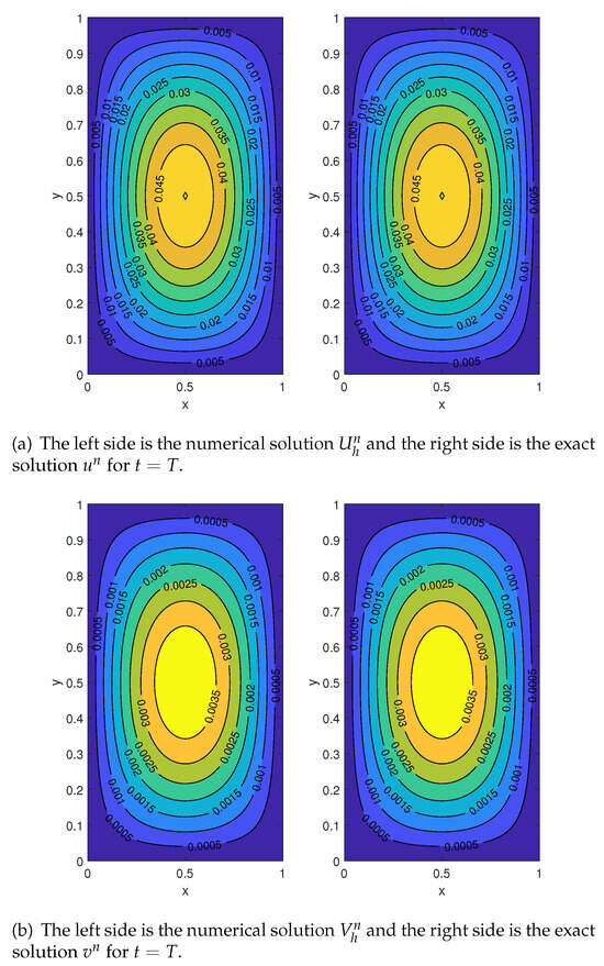
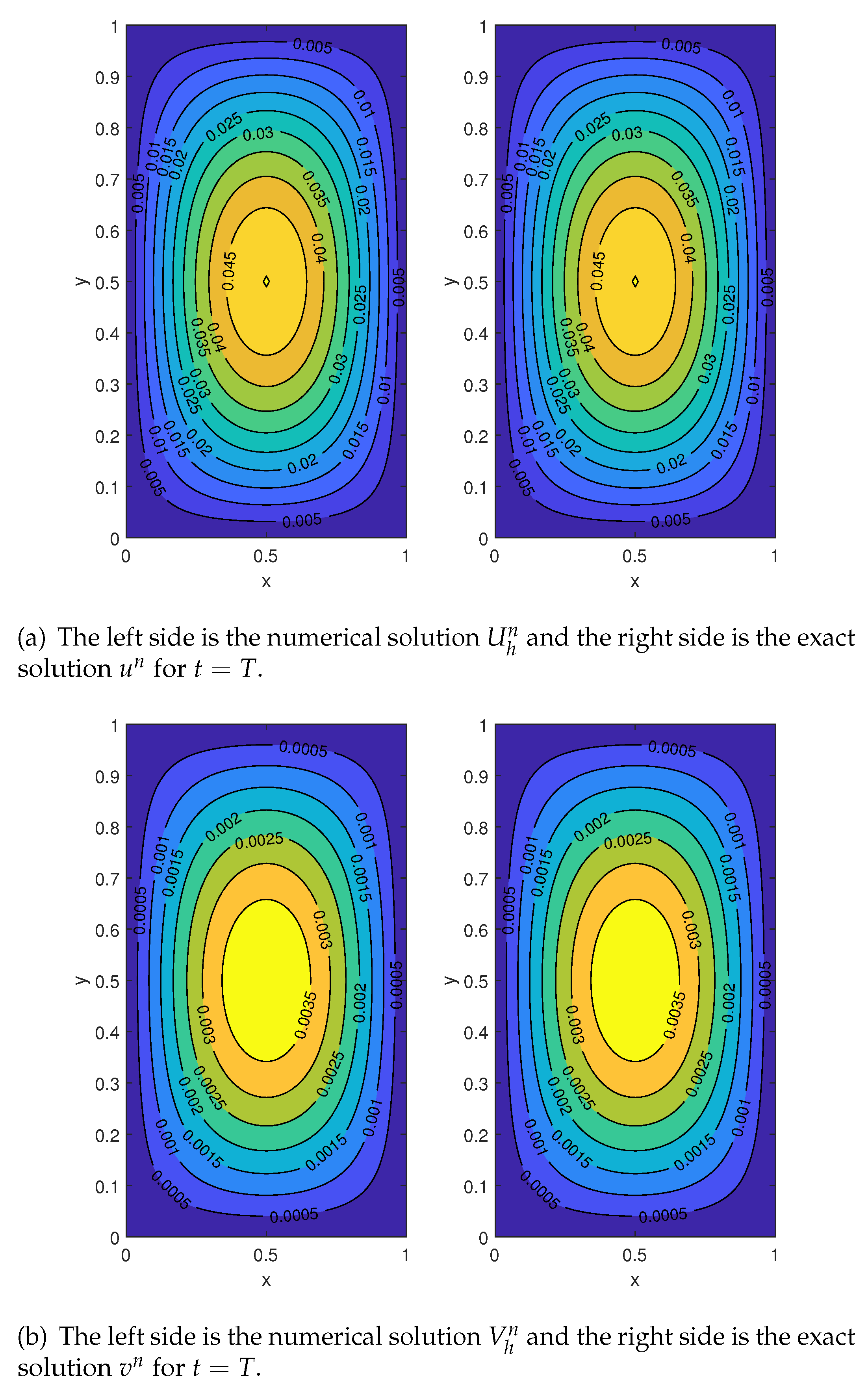
Taking the finial time $T={110}^{-3}$ and the time mesh parameter $r=6/\alpha$, the numerical solution and exact solution are shown in Figure 1, which are consistent. Here, we mainly consider the situation of $\alpha \to 1^{-}$. In Table 1, the spatial error convergence orders of $u,v$ are approximately 2 and 1 in the $L^2(\Omega )$ norm and the $H^1(\Omega )$ norm, respectively, which is consistent with Theorem 2. In addition, we provide the time error results of $u,v$ in the $L^2(\Omega )$ norm in Table 2. From the results, it can be seen that the error convergence order is close to 2, which is consistent with Theorem 3.

Figure 1. The comparison figures of the exact solution and the numerical solution with N = 100, $h={\displaystyle \frac{1}{64}},\alpha =0.8$ for Example 1.

Table 1. The spatial errors and convergence orders with the time steps $N=100$ for Example 1.

$\mathit{\alpha }$	h	$\parallel {\mathit{E}}_{\mathit{u}}\parallel$	Rate	$\parallel {\mathit{E}}_{\mathit{u}}{\parallel }_1$	Rate	$\parallel {\mathit{E}}_{\mathit{v}}\parallel$	Rate	$\parallel {\mathit{E}}_{\mathit{v}}{\parallel }_1$	Rate
0.8	$1/4$	1.3527 × 10−3	–	4.5514 × 10−2	–	1.0776 × 10−4	–	3.6208 × 10−3	–
	$1/8$	2.6193 × 10−4	2.3686	2.2136 × 10−2	1.0399	2.0876 × 10−5	2.3679	1.7614 × 10−3	1.0396
	$1/16$	5.9070 × 10−5	2.1487	1.0954 × 10−2	1.0149	4.6869 × 10−6	2.1551	8.7172 × 10−4	1.0148
	$1/32$	1.4979 × 10−5	1.9795	5.4615 × 10−3	1.0041	1.1450 × 10−6	2.0333	4.3463 × 10−4	1.0041
0.9	$1/4$	6.6022 × 10−4	–	2.3059 × 10−2	–	5.2545 × 10−5	–	1.8348 × 10−3	–
	$1/8$	1.2279 × 10−4	2.4267	1.1145 × 10−2	1.0490	9.7748 × 10−6	2.4264	8.8684 × 10−4	1.0489
	$1/16$	2.6402 × 10−5	2.2175	5.4992 × 10−3	1.0191	2.1014 × 10−6	2.2177	4.3761 × 10−4	1.0190
	$1/32$	6.3036 × 10−6	2.0664	2.7391 × 10−3	1.0055	4.9967 × 10−7	2.0723	2.1797 × 10−4	1.0055
0.95	$1/4$	4.6514 × 10−4	–	1.6385 × 10−2	–	3.7016 × 10−5	–	1.3038 × 10−3	–
	$1/8$	8.5618 × 10−5	2.4417	7.9053 × 10−3	1.0515	6.8140 × 10−6	2.4416	6.2907 × 10−4	1.0514
	$1/16$	1.8064 × 10−5	2.2448	3.8966 × 10−3	1.0206	1.4378 × 10−6	2.2447	3.1008 × 10−4	1.0206
	$1/32$	4.2409 × 10−6	2.0907	1.9399 × 10−3	1.0062	3.3717 × 10−7	2.0923	1.5437 × 10−4	1.0062

Table 2. The time errors and convergence orders with the spatial mesh size $h={\displaystyle \frac{1}{100}}$ for Example 1.

$\mathit{\alpha }$	N	$\parallel {\mathit{E}}_{\mathit{u}}\parallel$	Rate	$\parallel {\mathit{E}}_{\mathit{v}}\parallel$	Rate
0.8	4	4.6535 × 10−4	−	4.0864 × 10−5	−
	8	1.4175 × 10−4	1.7149	1.2460 × 10−5	1.7135
	16	3.7849 × 10−5	1.9051	3.2314 × 10−6	1.9471
	32	1.0781 × 10−5	1.8118	7.9979 × 10−7	2.0145
0.9	4	1.2799 × 10−4	−	1.0654 × 10−5	−
	8	3.8748 × 10−5	1.7238	3.2209 × 10−6	1.7258
	16	1.0290 × 10−5	1.9129	8.4453 × 10−7	1.9312
	32	2.7964 × 10−6	1.8796	2.1743 × 10−7	1.9576
0.95	4	4.6330 × 10−5	−	3.7983 × 10−6	−
	8	1.3992 × 10−5	1.7274	1.1443 × 10−6	1.7309
	16	3.7566 × 10−6	1.8971	3.0351 × 10−7	1.9147
	32	1.0897 × 10−6	1.7855	8.4279 × 10−8	1.8485

Finally, we provide a computing time comparison between the L2-1_σ scheme and the fast L2-1_σ scheme in Table 3, and we can see that the fast algorithm requires significantly less computation time.

Table 3. The computation time of the L2-1_σ/FEM and the fast L2-1_σ/FEM scheme with $h=1/8$, $\alpha =0.8$ for Example 1.

N	800	1000	1200	1400	1600
L2-1σ/FEM scheme	134.128 s	208.3286 s	338.0771 s	673.9065 s	900.8299 s
Fast L2-1σ/FEM scheme	94.9092 s	167.8129 s	222.4437 s	310.5037 s	328.4481 s

Example 2.

Assume that the domain $\Omega ={(0,1)}^2$; we then consider the non-smooth solutions are given by

$$u=\left\{\begin{array}{cc}5(t^2+t^{\alpha })xy(x-0.5)(y-1),\hfill & \mathit{in}{\Omega }_1,\hfill \\ (t^2+t^{\alpha })(x-0.5)(x-1)y(y-1),\hfill & \mathit{in}{\Omega }_2,\hfill \end{array}\right.$$

and

$$v=\left\{\begin{array}{cc}(t^2+t^{\alpha })xy(x-0.5)(y-1),\hfill & \mathit{in}{\Omega }_1,\hfill \\ 0.2(t^2+t^{\alpha })(x-0.5)(x-1)y(y-1),\hfill & \mathit{in}{\Omega }_2,\hfill \end{array}\right.$$

where ${\Omega }_1=[0,0.5]\times [0,1]$ and ${\Omega }_2=[0.5,1]\times [0,1]$.

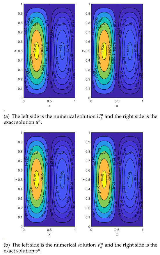
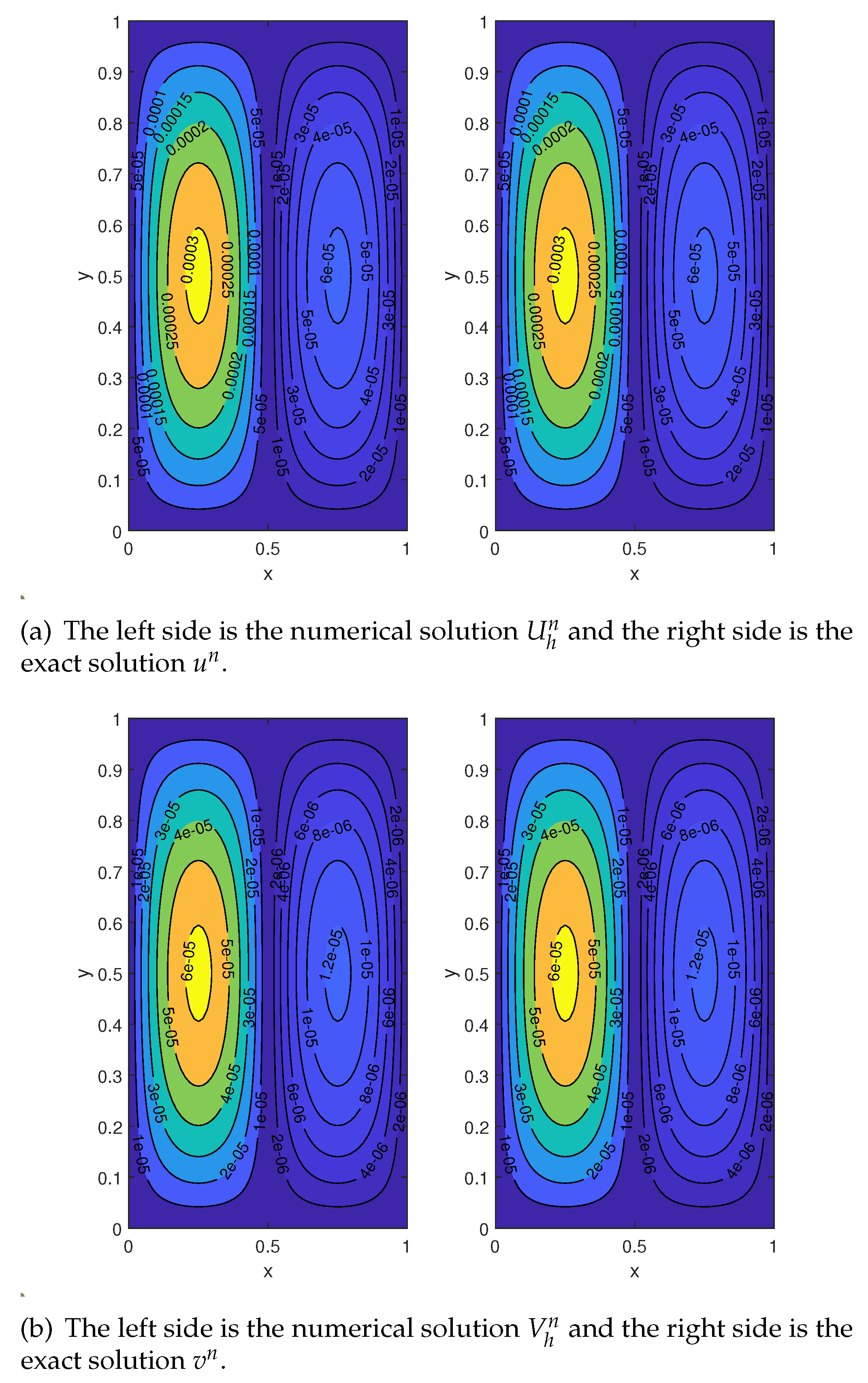
In the same way, we take the finial time T = 1 × 10⁻³ and the time mesh parameter $r=6/\alpha$. From Figure 2, it can be seen that the numerical solution is consistent with the exact solution. Based on the results in Table 4, we can also achieve the convergence orders of the second order and the first order in the $L^2(\Omega )$ norm and $H^1(\Omega )$ norm for the case of the non-smooth solutions. By comparing the data in Table 2, Table 5, and Table 6, it can be concluded that for the case of the non-smooth solutions, a finer spatial mesh discretization is required to achieve a temporal convergence order close to 2.

Figure 2. The comparison figures of the exact solution and the numerical solution for $N=100$, $h={\displaystyle \frac{1}{64}},\alpha =0.8$ for Example 2.

Table 4. The spatial errors and convergence orders with the time steps $N=100$ for Example 2.

$\mathit{\alpha }$	h	$\parallel {\mathit{E}}_{\mathit{u}}\parallel$	Rate	$\parallel {\mathit{E}}_{\mathit{u}}{\parallel }_1$	Rate	$\parallel {\mathit{E}}_{\mathit{v}}\parallel$	Rate	$\parallel {\mathit{E}}_{\mathit{v}}{\parallel }_1$	Rate
0.8	$1/4$	2.6299 × 10−5	–	6.3752 × 10−4	–	5.2618 × 10−6	–	1.2748 × 10−4	–
	$1/8$	5.2585 × 10−6	2.3223	3.1209 × 10−4	1.0305	1.0528 × 10−6	2.3213	6.2412 × 10−5	1.0303
	$1/16$	1.1810 × 10−6	2.1547	1.5406 × 10−4	1.0185	2.3662 × 10−7	2.1536	3.0811 × 10−5	1.0184
	$1/32$	2.8548 × 10−7	2.0485	7.6730 × 10−5	1.0056	5.7217 × 10−8	2.0481	1.5346 × 10−5	1.0056
0.9	$1/4$	1.2896 × 10−5	–	3.2526 × 10−4	–	2.5793 × 10−6	–	6.5049 × 10−5	–
	$1/8$	2.4591 × 10−6	2.3907	1.5789 × 10−4	1.0427	4.9192 × 10−7	2.3905	3.1577 × 10−5	1.0427
	$1/16$	5.2117 × 10−7	2.2383	7.7482 × 10−5	1.0270	1.0429 × 10−7	2.2379	1.5496 × 10−5	1.0269
	$1/32$	1.2231 × 10−7	2.0912	3.8500 × 10−5	1.0090	2.4481 × 10−8	2.0908	7.7001 × 10−6	1.0090
0.95	$1/4$	9.0968 × 10−6	–	2.3155 × 10−4	–	1.8194 × 10−6	–	4.6309 × 10−5	–
	$1/8$	1.7121 × 10−6	2.4096	1.1223 × 10−4	1.0449	3.4244 × 10−7	2.4095	2.2446 × 10−5	1.0448
	$1/16$	3.5306 × 10−7	2.2778	5.4960 × 10−5	1.0301	7.0629 × 10−8	2.2775	1.0992 × 10−5	1.0300
	$1/32$	8.1251 × 10−8	2.1195	2.7276 × 10−5	1.0107	1.6257 × 10−8	2.1192	5.4552 × 10−6	1.0107

Table 5. The time errors and convergence orders with the spatial mesh size $h={\displaystyle \frac{1}{100}}$ for Example 2.

$\mathit{\alpha }$	N	$\parallel {\mathit{E}}_{\mathit{u}}\parallel$	Rate	$\parallel {\mathit{E}}_{\mathit{v}}\parallel$	Rate
0.8	4	1.9447 × 10−6	–	4.0582 × 10−7	–
	8	5.7268 × 10−7	1.7637	1.2009 × 10−7	1.7567
	16	1.5138 × 10−7	1.9195	3.1711 × 10−8	1.9211
	32	4.9146 × 10−8	1.6231	1.0095 × 10−8	1.6513
0.9	4	6.3564 × 10−7	–	1.2934 × 10−7	–
	8	1.9213 × 10−7	1.7261	3.9116 × 10−8	1.7253
	16	5.2613 × 10−8	1.8686	1.0696 × 10−8	1.8707
	32	1.8532 × 10−8	1.5054	3.7373 × 10−9	1.5170
0.95	4	2.4057 × 10−7	–	4.8654 × 10−8	–
	8	7.3227 × 10−8	1.7160	1.4809 × 10−8	1.7161
	16	2.1337 × 10−8	1.7790	4.3061 × 10−9	1.7820
	32	9.8102 × 10−9	1.1210	1.9678 × 10−9	1.1298

Table 6. The time errors and convergence orders with the spatial mesh size $h={\displaystyle \frac{1}{200}}$ for Example 2.

$\mathit{\alpha }$	N	$\parallel {\mathit{E}}_{\mathit{u}}\parallel$	Rate	$\parallel {\mathit{E}}_{\mathit{v}}\parallel$	Rate
0.8	4	1.9387 × 10−6	–	4.046 × 10−7	–
	8	5.6607 × 10−7	1.7760	1.1876 × 10−7	1.7685
	16	1.4301 × 10−7	1.9849	3.0036 × 10−8	1.9832
	32	3.539 × 10−8	2.0147	7.3613 × 10−9	2.0287
0.9	4	6.3406 × 10−7	–	1.2902 × 10−7	–
	8	1.9028 × 10−7	1.7365	3.8746 × 10−8	1.7355
	16	4.9802 × 10−8	1.9338	1.0136 × 10−8	1.9345
	32	1.2933 × 10−8	1.9452	2.6221 × 10−9	1.9508
0.95	4	2.3972 × 10−7	–	4.8484 × 10−8	–
	8	7.2087 × 10−8	1.7335	1.4581 × 10−8	1.7334
	16	1.9153 × 10−8	1.9122	3.8711 × 10−9	1.9133
	32	5.3333 × 10−9	1.8444	1.0739 × 10−9	1.8499

6. Conclusions

This work presents present a fast L2-1_σ/FEM scheme for solving the time fractional Keller–Segel equations with weakly singular solutions. Based on an improved fractional Grönwall inequality, we establish stability and the $\alpha$ robust error estimates for the numerical formats. Finally, some numerical examples are presented to illustrate the reliability of our algorithms and the correctness of our theoretical results. However, there are still some minor flaws here, such as the small final time of our numerical simulation. For this problem, we will further study the blow-up of the numerical solution to derive a long-term numerical simulation.

References

- Magin, R.L. Fractional calculus models of complex dynamics in biological tissues. Comput. Math. Appl. 2010, 59, 1586–1593. [Google Scholar] [CrossRef] [Scilit]
- Hilfer, R. Applications of Fractional Calculus in Physics; World Scientific: Singapore, 2000. [Google Scholar]
- Caponetto, R.; Dongola, G.; Fortuna, L.; Petras, I. Fractional Order Systems: Modeling and Control Applications; World Scientific: Singapore, 2010; Volume 72. [Google Scholar]
- Lord, R.; Fang, F.; Bervoets, F.; Oosterlee, C.W. A fast and accurate FFT-based method for pricing early-exercise options under Lévy processes. SIAM J. Sci. Comput. 2008, 30, 1678–1705. [Google Scholar] [CrossRef] [Scilit]
- Keller, E.F.; Segel, L.A. Initiation of slime mold aggregation viewed as an instability. J. Theor. Biol. 1970, 26, 399–415. [Google Scholar] [CrossRef] [Scilit]
- Keller, E.F.; Segel, L.A. Traveling bands of chemotactic bacteria: A theoretical analysis. J. Theor. Biol. 1971, 30, 235–248. [Google Scholar] [CrossRef] [Scilit]
- Haastert, P.J.M.V.; Devreotes, P.N. Chemotaxis: Signalling the way forward. Nat. Rev. Mol. Cell Biol. 2004, 5, 626–634. [Google Scholar] [CrossRef] [Scilit] [PubMed]
- Hillen, T.; Painter, K.J. A user’s guide to PDE models for chemotaxis. J. Math. Biol. 2009, 58, 183–217. [Google Scholar] [CrossRef] [Scilit]
- Eisenbach, M. Chemotaxis; World Scientific Publishing Company: Singapore, 2004. [Google Scholar]
- Feder, T.J.; Brust-Mascher, I.; Slattery, J.P.; Baird, B.; Webb, W.W. Constrained diffusion or immobile fraction on cell surfaces: A new interpretation. Biophys. J. 1996, 70, 2767–2773. [Google Scholar] [CrossRef] [Scilit]
- Banks, D.S.; Fradin, C. Anomalous diffusion of proteins due to molecular crowding. Biophys. J. 2005, 89, 2960–2971. [Google Scholar] [CrossRef] [Scilit]
- Weiss, M.; Hashimoto, H.; Nilsson, T. Anomalous protein diffusion in living cells as seen by fluorescence correlation spectroscopy. Biophys. J. 2003, 84, 4043–4052. [Google Scholar] [CrossRef] [Scilit]
- Metzler, R.; Klafter, J. The random walk’s guide to anomalous diffusion: A fractional dynamics approach. Phys. Rep. 2000, 339, 1–77. [Google Scholar] [CrossRef] [Scilit]
- Langlands, T.A.M.; Henry, B.I. Fractional chemotaxis diffusion equations. Phys. Rev. E 2010, 81, 051102. [Google Scholar] [CrossRef] [Scilit] [PubMed]
- Naghibolhosseini, M. Estimation of Outer-Middle Ear Transmission Using DPOAEs and Fractional-Order Modeling of Human Middle Ear. Ph.D. Thesis, City University of New York, New York, NY, USA, 2015. [Google Scholar]
- Li, L.; Liu, J.G. Some compactness criteria for weak solutions of time fractional PDEs. SIAM J. Math. Anal. 2018, 50, 3963–3995. [Google Scholar] [CrossRef] [Scilit]
- Zhou, Y.; Manimaran, J.; Shangerganesh, L.; Debbouche, A. Weakness and Mittag–Leffler stability of solutions for time-fractional Keller–Segel models. Int. J. Nonlinear Sci. Numer. Simul. 2018, 19, 753–761. [Google Scholar] [CrossRef] [Scilit]
- Aruchamy, A.; Tyagi, J. Nonnegative solutions to time fractional Keller–Segel system. Math. Methods Appl. Sci. 2021, 44, 1812–1830. [Google Scholar] [CrossRef] [Scilit]
- Bezerra, M.; Cuevas, C.; Silva, C.; Soto, H. On the fractional doubly parabolic Keller-Segel system modelling chemotaxis. Sci. China Math. 2022, 65, 1827–1874. [Google Scholar] [CrossRef] [Scilit]
- Costa, M.; Cuevas, C.; Silva, C.; Soto, H. Well-posedness and blow-up of the fractional Keller–Segel model on domains. Math. Nachrichten 2023, 296, 5569–5592. [Google Scholar] [CrossRef] [Scilit]
- El-Sayed, A.M.A.; Rida, S.Z.; Arafa, A.A.M. On the solutions of time-fractional bacterial chemotaxis in a diffusion gradient chamber. Int. J. Nonlinear Sci. 2009, 7, 485–492. [Google Scholar]
- Kumar, S.; Kumar, A.; Argyros, I.K. A new analysis for the Keller–Segel model of fractional order. Numer. Algorithms 2017, 75, 213–228. [Google Scholar] [CrossRef] [Scilit]
- Dokuyucu, M.A.; Baleanu, D.; Çelik, E. Analysis of Keller–Segel model with Atangana-Baleanu fractional derivative. Filomat 2018, 32, 5633–5643. [Google Scholar] [CrossRef] [Scilit]
- Morales-Delgado, V.F.; Gómez-Aguilar, J.F.; Kumar, S.; Taneco-Hernández, M.A. Analytical solutions of the Keller–Segel chemotaxis model involving fractional operators without singular kernel. Eur. Phys. J. Plus 2018, 133, 200. [Google Scholar] [CrossRef] [Scilit]
- Nguyen, A.T.; Tuan, N.H.; Yang, C. On cauchy problem for fractional parabolic-elliptic Keller–Segel model. Adv. Nonlinear Anal. 2022, 12, 97–116. [Google Scholar] [CrossRef] [Scilit]
- Khaider, H.; El-Ouaarabi, M.; Raji, A. An Global existence and uniqueness of mild solution for a fractional Keller-Segel system in Besov-Morrey spaces. Math. Model. Anal. 2025, 30, 685–706. [Google Scholar] [CrossRef] [Scilit]
- Zayernouri, M.; Matzavinos, A. Fractional Adams–Bashforth/Moulton methods: An application to the fractional Keller–Segel chemotaxis system. J. Comput. Phys. 2016, 317, 1–14. [Google Scholar] [CrossRef] [Scilit]
- Sakamoto, K.; Yamamoto, M. Initial value/boundary value problems for fractional diffusion-wave equations and applications to some inverse problems. J. Math. Anal. Appl. 2011, 382, 426–447. [Google Scholar] [CrossRef] [Scilit]
- Stynes, M.; O’Riordan, E.; Gracia, J.L. Error analysis of a finite difference method on graded meshes for a time-fractional diffusion equation. SIAM J. Numer. Anal. 2017, 55, 1057–1079. [Google Scholar] [CrossRef] [Scilit]
- Liao, H.L.; Li, D.F.; Zhang, J.W. Sharp error estimate of the nonuniform L1 formula for linear reaction-subdiffusion equations. SIAM J. Numer. Anal. 2018, 56, 1112–1133. [Google Scholar] [CrossRef] [Scilit]
- Kopteva, N. Error analysis of the L1 method on graded and uniform meshes for a fractional-derivative problem in two and three dimensions. Math. Comput. 2019, 88, 2135–2155. [Google Scholar] [CrossRef] [Scilit]
- Chen, H.; Stynes, M. Error analysis of a second-order method on fitted meshes for a time-fractional diffusion problem. J. Sci. Comput. 2019, 79, 624–647. [Google Scholar] [CrossRef] [Scilit]
- Kopteva, N. Error analysis of an L2-type method on graded meshes for a fractional-order parabolic problem. Math. Comput. 2021, 90, 19–40. [Google Scholar] [CrossRef] [Scilit]
- Huang, C.B.; Stynes, M. A sharp α-robust L∞(H1) error bound for a time-fractional Allen–Cahn problem discretised by the Alikhanov L2-1σ scheme and a standard FEM. J. Sci. Comput. 2022, 91, 43. [Google Scholar] [CrossRef] [Scilit]
- Mustapha, K.; Abdallah, B.; Furati, K.M. A discontinuous Petrov–Galerkin method for time-fractional diffusion equations. SIAM J. Numer. Anal. 2014, 52, 2512–2529. [Google Scholar] [CrossRef] [Scilit]
- Jin, B.T.; Li, B.Y.; Zhou, Z. Correction of high-order bdf convolution quadrature for fractional evolution equations. SIAM J. Sci. Comput. 2017, 39, A3129–A3152. [Google Scholar] [CrossRef] [Scilit]
- Jin, B.T.; Li, B.Y.; Zhou, Z. Subdiffusion with time-dependent coefficients: Improved regularity and second-order time stepping. Numer. Math. 2020, 145, 883–913. [Google Scholar] [CrossRef] [Scilit]
- Xing, Y.Y.; Yan, Y.B. A higher order numerical method for time fractional partial differential equations with nonsmooth data. J. Comput. Phys. 2018, 357, 305–323. [Google Scholar] [CrossRef] [Scilit]
- Yan, Y.B.; Khan, M.; Ford, N.J. An analysis of the modified L1 scheme for time-fractional partial differential equations with nonsmooth data. SIAM J. Numer. Anal. 2018, 56, 210–227. [Google Scholar] [CrossRef] [Scilit]
- Jiang, S.D.; Zhang, J.W.; Zhang, Q.; Zhang, Z.M. Fast evaluation of the Caputo fractional derivative and its applications to fractional diffusion equations. Commun. Comput. Phys. 2017, 21, 650–678. [Google Scholar] [CrossRef] [Scilit]
- Liao, H.L.; Yan, Y.G.; Zhang, J.W. Unconditional convergence of a fast two-level linearized algorithm for semilinear subdiffusion equations. J. Sci. Comput. 2019, 80, 1–25. [Google Scholar] [CrossRef] [Scilit]
- Yan, Y.G.; Sun, Z.Z.; Zhang, J.W. Fast evaluation of the Caputo fractional derivative and its applications to fractional diffusion equations: A second-order scheme. Commun. Comput. Phys. 2017, 22, 1028–1048. [Google Scholar] [CrossRef] [Scilit]
- Zhu, H.Y.; Xu, C.J. A fast high order method for the time-fractional diffusion equation. SIAM J. Numer. Anal. 2019, 57, 2829–2849. [Google Scholar] [CrossRef] [Scilit]
- Liu, N.; Chen, Y.P.; Zhang, J.W.; Zhao, Y.M. Unconditionally optimal h 1-error estimate of a fast nonuniform L2-1σ scheme for nonlinear subdiffusion equations. Numer. Algorithms 2023, 92, 1655–1677. [Google Scholar] [CrossRef] [Scilit]
- Li, Q.; Xie, J. A fast second order PDE approach for the space-time fractional parabolic problems. AIMS Math. 2025, 10, 25568–25588. [Google Scholar] [CrossRef] [Scilit]
- Zeng, Y.; Tan, Z. An α-robust two-grid finite element method with nonuniform L2-1Σ scheme for the semilinear Caputo-Hadamard time-fractional diffusion equations involving initial singularity. Appl. Math. Comput. 2025, 496, 129355. [Google Scholar]
- Garrappa, R.; Moret, I.; Popolizio, M. Solving the time-fractional Schrödinger equation by Krylov projection methods. J. Comput. Phys. 2015, 293, 115–134. [Google Scholar] [CrossRef] [Scilit]
- Alikhanov, A.A. A new difference scheme for the time fractional diffusion equation. J. Comput. Phys. 2015, 280, 424–438. [Google Scholar] [CrossRef] [Scilit]
- Li, X.; Liao, H.L.; Zhang, L.M. A second-order fast compact scheme with unequal time-steps for subdiffusion problems. Numer. Algorithms 2021, 86, 1011–1039. [Google Scholar] [CrossRef] [Scilit]
- Wang, Y.B.; An, N.; Huang, C.B. Unconditional optimal error bounds of the fast nonuniform Alikhanov scheme for a nonlinear time-fractional biharmonic equation. J. Appl. Math. Comput. 2024, 70, 4053–4071. [Google Scholar] [CrossRef] [Scilit]
- Thomée, V. Galerkin Finite Element Methods for Parabolic Problems; Springer Science & Business Media: Berlin/Heidelberg, Germany, 2007; Volume 25. [Google Scholar]
- Chen, H.; Stynes, M. Blow-up of error estimates in time-fractional initial-boundary value problems. IMA J. Numer. Anal. 2021, 41, 974–997. [Google Scholar] [CrossRef] [Scilit]
Disclaimer/Publisher’s Note: The statements, opinions and data contained in all publications are solely those of the individual author(s) and contributor(s) and not of MDPI and/or the editor(s). MDPI and/or the editor(s) disclaim responsibility for any injury to people or property resulting from any ideas, methods, instructions or products referred to in the content. |
© 2026 by the authors. Licensee MDPI, Basel, Switzerland. This article is an open access article distributed under the terms and conditions of the Creative Commons Attribution (CC BY) license.