


Abstract
Finite-precision chaotic generators are deterministic finite-state systems whose structure is not established by continuous-domain chaos indicators or by ciphertext statistics. We study a map on coupled to a Weyl counter and prove that every eventual joint cycle length is divisible by the counter period, while the image fraction and the normalized indegree distribution are preserved exactly. A simple instance attains this period floor and is predictable from two words of its own output. We then audit fifteen specified quantized realizations, thirteen from recent image-encryption designs and classical maps and two validation controls, under two quantizers at reduced widths, measuring reachability, recurrence, cycle-length distributions and output-equivalence classes. An exponential enhancer that improves every dynamical indicator its authors report lowers the image fraction for three of its four base maps and raises it for the fourth. Across the sampled one-dimensional cases the section-cycle multiplier is at most three, while the two- and three-dimensional examples reach the tens; a permutation counterexample rules out a universal dimension-based claim. Under the common post-update decimal readout, the non-affine one-dimensional realizations approach the image-size bound within six output symbols. These findings motivate reporting finite-state structure alongside conventional tests. The measurements characterize the specified reduced-width realizations; they neither establish native-precision behaviour nor prove or disprove the security of the source ciphers.
1. Introduction
Chaos-based image encryption has a settled evidentiary convention. A paper proposing a map establishes that the map is chaotic, with bifurcation diagrams, Lyapunov exponents, entropy measures and the 0–1 test; a paper proposing a scheme establishes that its ciphertext is statistically unremarkable, with entropy, adjacent-pixel correlation, NPCR, UACI, key space and a robustness study. The convention is followed carefully.
It has a gap, and the gap is structural rather than a matter of rigour. The first group of quantities describes a map on the reals or the torus, the second the output of a completed scheme. Neither describes the object that runs, which is a map on a finite set of machine words with a functional graph, a reachable set, a distribution of cycle lengths and a set of states that nothing maps to. A map can have a positive Lyapunov exponent and near-maximal entropy while its digital realization reaches under half its state space in one step, so that the state diversity available to a downstream key stream or permutation stage is far smaller than the word width suggests. Those quantities are cheap to compute exactly at reduced precision, and none of the design papers we survey in Section 2 reports them; we make that claim about those papers, which we read in full, and not about the literature at large.
That the gap matters has been argued from the cryptanalytic side. Singh et al. [1] recover plaintext from a chaos-based multi-image scheme under a ciphertext-only attack and conclude that statistical validation is no substitute for security analysis. Their remedy is deeper security analysis; ours is narrower. Before asking whether a construction resists attack, one can ask what its state graph looks like, and that question has exact answers.
That finite precision degrades chaotic maps is itself long established [2], the finite-state object has been analysed directly as a state-mapping network [3,4], and Weyl sequences are a standard device for imposing a period floor on a generator [5,6,7]. What we did not find stated, having read those works rather than searched systematically, is the preservation identity itself: that period extension by a counter and state-space reachability are independent, so that a construction can fix the first while provably leaving the second exactly as it was. That identity, the audit protocol built on it, and the comparative measurements of Section 4 are what we offer as new.
This paper proceeds in two parts. We study a construction that couples an arbitrary map to a Weyl counter, prove what it guarantees and prove what it leaves untouched, and give an instance showing that the guarantee carries no implication for the output. We then measure, rather than argue about, fifteen maps, including those of four recent designs, re-implemented from their published equations, at the parameters recorded in Appendix A.3 where the sources fix them and at our own selections where they do not, and enumerated exhaustively as quantized realizations at reduced word width. The measurements follow a written analysis plan; that plan, its three amendments, their digests and the records are in the artifact, every reported figure is generated from a record rather than transcribed, and experiments added by amendment are labelled exploratory.
Contributions
- A construction with a proved period floor [P]. Definition 1 couples an arbitrary map T on to a Weyl counter injected into one word; Theorem 1 shows every eventual joint cycle has length divisible by , with no hypothesis on the map, and Proposition 1 shows nothing about the output follows.
- A proof that the coupling does not touch injectivity [P]. Proposition 2 shows the joint map has the same preimage-size distribution as T, so image fraction, unreached states and fibre structure are inherited exactly. Taken with the first contribution, this is the paper’s organizing point: the counter settles the period and settles nothing about reachability.
- An audit of fifteen specified quantized realizations [E], including the maps of four recent designs, reporting image fraction, cyclic fraction, cycle multisets, tails and output-equivalence classes at widths from 12 to 30 bits under two quantizers. Two findings carry the argument. Conventional dynamical and ciphertext statistics do not track any of these: the enhancer of [8] improves every quantity its authors report while lowering the image fraction over three of its four base maps. And what a counter contributes to the period is separable from what the map contributes, which we measure rather than assume; the observed pattern is a property of the maps and widths tested, not a theorem about dimension, as an explicit one-dimensional permutation shows (Section 4.6).
The measurements are implementation diagnostics. Their cryptographic implications depend on initialization, observation and the adversary model, and they establish neither the security nor the insecurity of the source ciphers. No map studied here is asserted secure or insecure, a longer period is not asserted to be an improvement, and the maps are not ranked; two of those we measure have higher image fractions than our own validation instances, which we report as measured. The claim is that the ordering produced by the published metrics is not the ordering produced by finite-state measurement, and that the surveyed designs report only the first.
Section 2 sets out the convention, including designs of our own that follow it. Section 3 gives the construction and its guarantees, Section 4 the enumeration, and Section 6 what we propose be reported instead. Figure 1 lays the whole of it out on one page: the object enumerated, the three quantities read from it, and the two reference lines each is read against.
Figure 1.
What the audit measures, and against what. Once a chaotic map is quantized, the key stream of an image cipher comes from a function on w-bit words: a finite object with a functional graph, in which every state lies on a cycle, drains into one, or has no predecessor. The left panel draws that graph for the logistic realization at , where all 128 states fit: filled red marks a state on a cycle, grey a state that is reached but transient, and hollow a state no state maps to; four are cyclic and 72 are unreached. The audit enumerates the graph exhaustively and reports three quantities (centre): the image fraction (Section 4.4), the cyclic fraction (Section 4.10 at , Table S4 at ) and the number of distinguishable key streams (Section 4.10). Each is read against a bijection, which a block cipher or counter-mode PRF attains by construction, and a uniform random map (right; Section 4.2). The nine one-dimensional maps of Section 4.12 reach to of their states in one step at (Section 4.3); fewer than one state in five hundred ever recurs for any of them at , and their distinguishable key streams meet the image-fraction bound within six emitted words. None of the observables is a security level: is the advantage of a one-query membership distinguisher (Proposition 3), and no cipher is proposed. Every measured value is exact at a reduced word width, and none describes a generator running in binary64; Section 6.4 sets out what carries over from the tested widths.
2. Related Work
2.1. What Recent Designs Report
Chaotic image encryption has a settled evidentiary convention, and the four recent designs below follow it closely.
Li, Li and Di [8] introduce an exponential factor to repair the loss of chaotic behaviour that cosine-type enhancers show as the control parameter approaches zero, supporting it with bifurcation diagrams, Lyapunov exponents, sample entropy and the 0–1 test over four classical one-dimensional maps. Pandey and Sharma [9] pair a Lorenz system with a logistic–piecewise-linear hybrid, then encrypt with elliptic-curve cryptography and optimise the cipher image with a genetic algorithm, supporting the hybrid with a bifurcation diagram and a Lyapunov plot. Deepankumar et al. [10] adopt a three-dimensional logistic map, arguing for it from the key space that six double-precision parameters provide and from the visibly more uniform trajectory distribution, and evaluate with entropy, correlation, chi-square, NIST SP 800-22, NPCR, UACI and robustness tests. Liu et al. [11] cross-couple Chebyshev and cubic maps and add Kolmogorov and permutation entropy to the same battery; their introduction states the problem this paper takes up most directly, naming dynamic degradation under finite precision as an inherent limitation of one-dimensional maps and offering a two-dimensional construction as the answer.
The pattern is uniform. Every paper establishes that its map is chaotic on a continuous idealisation, then that the cipher built on it produces statistically unremarkable ciphertext. Neither is a statement about the finite state machine that runs, and none of the four surveyed papers reports the period of that machine, the size of its reachable set, or how much of its state space recurs. We make that claim about the studies surveyed here, not about the literature as a whole. Where finite-precision degradation is named, as in [8,11], the response is a design change justified by the same continuous-domain evidence rather than a measurement of the resulting state graph.
The convention is not confined to those four, and we do not exempt ourselves from it. Colour-image and key-generation schemes of ours [12,13,14,15] are evaluated on the same terms: MSE, PSNR, correlation, key sensitivity, throughput, occlusion robustness, entropy, NPCR, UACI, the NIST battery and a key space, and none reports the period, reachable set or cyclic structure of the map it iterates. A dynamical indicator measured on a stated grid, such as a Lyapunov spectrum with its degeneracy windows guarded at run time, would go further in one respect and no further in the other: it is still evidence about the continuous map. Section 4.2 uses a bijective counter transition as a structural reference, and the keyed output function is a separate object from the generator that drives it.
The omission is not incidental. The map underlying [12] is the logistic map at , a subject of Section 4: at its image fraction is , stable to three decimals across all six widths and both quantizers, so more than half its state space is unreachable in one step and the observation would have cost seconds. We include these papers because the argument is about a convention rather than about particular groups, and because we have followed that convention and can now say what it left out.
2.2. Chaos-Based Cryptography and Its Critics
Chaos-based encryption begins with Baptista’s symbolic cipher [16] and Fridrich’s permutation–diffusion construction [17], whose architecture almost every scheme surveyed above still follows; Chen, Mao and Chui [18] extended it to three-dimensional cat maps, and Dachselt and Schwarz [19] set out the correspondence between chaotic and cryptographic properties that motivated the field.
The critical literature is as old as the constructive one and is more directly relevant here. Alvarez and Li [20] give basic requirements for chaos-based cryptosystems and observe that proposed schemes seldom carry a thorough security analysis, recommending among other things that a designer study the parameter regions actually used. Alvarez, Amigó, Arroyo and Li [21], Solak [22] and Amigó, Kocarev and Szczepanski [23] collect the recurring failure modes and the gap between the theory of chaotic maps and the practice of building ciphers from them. Preishuber, Hütter, Katzenbeisser and Uhl [24] put the point empirically: the statistical batteries customarily used to argue for chaos-based image encryption fail to discriminate between secure and insecure constructions, so passing them is weak evidence. Singh et al. [1] make it concretely, recovering plaintext from a cross-coupled PWLCM multi-image scheme under a ciphertext-only attack and listing several chaos-based cryptosystems broken after passing exactly such evaluation; individual schemes continue to be broken by exploiting structure the published evaluation did not report [25,26].
Our position within that tradition is narrow. Their remedy is in-depth security analysis, which is not what this paper offers. We do not argue that chaotic maps are unsuitable for cryptographic use, and we break nothing. We observe that the evaluations at issue are computed on the continuous map or on cipher output, and that a third object, the quantized realization, admits exact and cheap measurements that none of the four surveyed papers reports. In Alvarez and Li’s terms, this supplies one of the implementation-level checks their guidelines call for.
2.3. Finite-State Structure of Digital Chaotic Maps
That digital chaotic maps degrade under fixed-point arithmetic is long established. Li, Chen and Mou [2] analyse the effect for piecewise linear maps and show that finite precision shortens periods and biases distributions in ways the continuous model does not predict.
The finite-state object itself has also been studied directly, and we do not claim otherwise. Li, Feng, Li, Kurths and Chen [3] analyse digital chaotic maps as state-mapping networks, in which every value of the digital domain is a node and every mapping relation a directed edge. That is the same object we enumerate, and the correspondence with our observables should be stated plainly: their inaccessible nodes are the complement of , so their density is ; their indegree distribution is the fibre-size distribution of Section 3, which Proposition 2 shows the counter preserves in normalized form; and the scale-free property they prove for the logistic map’s network is a statement about the tail of that same distribution. We take the object and the vocabulary from them and claim neither. Fan and Ding [4] give an algorithm for locating periodic cycles in such graphs, which is the computation behind our cyclic fraction. What these works do not do is apply the observables comparatively to the maps that recent image-encryption designs actually propose, or separate a period guarantee from the one-step collision structure it leaves untouched, which is what this paper adds.
Counter-based remedies are familiar outside this literature, where adding a Weyl sequence to a state is a known device for imposing a period floor on a generator, and the argument of Theorem 1 is essentially the one that justifies them. Three constructions are close enough to ours that the differences are worth stating rather than left implicit. Widynski’s middle-square Weyl sequence generator [5] squares a state, adds a separately evolving Weyl value, rotates the result and outputs its middle bits; his Squares generator [6] makes the counter the sole input of a keyed round function; Działa’s Collatz–Weyl generators [7] combine a generalized Collatz mapping with a Weyl sequence to obtain long periods and a parameterized family of streams. Ours is the explicit joint transition with a separately evolving counter. As in these constructions the injected value affects subsequent nonlinear updates, since ; the differences are in the wrapper, which adds a counter translation without prescribing an internal map or an output scrambler, and in what is analysed. None of these works reports the image fraction, indegree distribution or cyclic fraction of the resulting finite-state map. What we take from them is that the period floor is standard; what we add is the fibre-preservation identity for this specified transition and its use in a comparative audit, and we claim no new principle of Weyl-based period extension.
The statistics of the objects we measure are also classical. Flajolet and Odlyzko [27] give the limiting behaviour of random mappings on N points: image fraction , about cycles, and a longest cycle of order . We use those results as a reference scale, not as a validated model of the objects measured here.
Period structure has also been studied exactly for particular families rather than measured: Chen, Wong, Liao and Xiang [28] derive the period distribution of the generalized discrete Arnold cat map, which is the kind of closed-form result our Propositions 5 and 6 provide for the affine class and which we do not claim for the maps we measure.
Against that background we state our position narrowly. Graph enumeration of digital chaotic maps is not new [3,4], exact period results for structured families are not new [28], and counter-based period extension is not new [6]. What we add is the combination applied to a specific question: an exact identity relating the one-step collision structure of a coupled map to that of its base (Proposition 2), measured jointly with recurrence and readout-dependent output equivalence, for the quantized realizations that recent image-encryption designs actually specify. Table 1 sets out which of these elements appear in the closest prior work.
Table 1.
Elements of the present audit against the closest prior work. A check marks that the element is present, not that it is treated in the same way. A dash means we did not find the element in that work; it is a judgement from our reading of the cited paper, not a claim that the authors considered and rejected it. The middle-square and Collatz–Weyl generators of Section 2 are not rows here because they analyse period rather than any of the five columns; the counter-based generator of [6] is a row, since it states its finite-state semantics and perturbs by a counter; the “partial” for [3] under image/indegree reflects that its indegree statistics are reported for the logistic and tent maps rather than comparatively across proposed designs.
3. Construction and Finite-State Guarantees
Throughout, is the dimension, the word length in bits, and all arithmetic is modulo . The state space is , of size , and is the first standard basis vector. Each result carries a label, and the label is part of the claim: [P] for a statement proved here, [E] for an empirical result, exhaustive or sampled as each experiment states, [S] for agreement between independent implementations, and [H] for a heuristic model that is neither proved nor exhaustively checked and is offered only as an account of orders of magnitude. What each [P] result licenses downstream is stated once, at the end of this section, so that no later section can inherit a security claim from a structural theorem.
The paper measures several distinct objects, and confusing them is the easiest way to over-read a result. Table 2 names each and says where it appears; the Weyl coupling of Definition 1 is introduced as an analytical device for separating a guaranteed period from an inherited one-step structure, not as a proposed generator, and nothing in the paper should be read as recommending it for use.
Table 2.
The objects this paper measures, and the symbols used for each. Every result names one of them; none of the rows is a proxy for another.
3.1. The Construction
Definition 1
(Weyl coupling). Let be any deterministic map and let be odd. The coupled system has joint state and update
We write for the joint map.
The counter enters one word rather than all d. Injecting into every word would make two states differing only in their counter differ by the same known value in every coordinate, an exactly known relation across the whole state; injecting into a single word leaves the map’s own coupling to propagate it. Theorem 1 is indifferent to the choice, since it depends only on the counter component, so the decision rests on this reasoning alone and is recorded as a design choice rather than a derived one.
Where the construction is keyed, is derived from the key schedule under its own label, with the w-bit expansion under a label distinct from every other use of the key, so that it is a deterministic function of the key and a public label and contributes no independent key material. This paper studies the construction independently of any keying: no cipher is proposed and no key-space claim is made. Each run in Section 4 fixes explicitly and records it, and Section 4.9 varies it.
3.2. Period
Theorem 1
(Counter-period divisibility, [P]). Let T be any map on and let have 2-adic valuation . Every cycle of Φ has length divisible by , so the trajectory from any initial state eventually enters a cycle at least that long. For odd γ the bound is . (A transient state need not return to itself, so the statement is about eventual cycle length, not about return to the initial state.)
Proof.
The counter component evolves independently of X as on , so is a coset of the subgroup generated by and has exact period . If the joint state returns after P steps then in particular , so P is a multiple of that period. No property of T was used. □
Definition 1 requires odd and every experiment below uses an odd increment; the theorem is stated for general only to make the cost of a poor choice explicit. An increment divisible by shortens the guaranteed cycle by a factor . That is a loss of guaranteed period, not of security bits: the two are different quantities.
Proposition 1
(The floor does not reach the output, [P]). Let be any extractor of the -component alone, let , let P be the eventual period of the joint state and the eventual period of . Then , and Theorem 1 entails no non-trivial lower bound on and no statement about the predictability of . The restriction to the -component is deliberate and is the case a deployed generator matches: the counter is bookkeeping and is not emitted. A readout of the full joint state, , would satisfy the same divisibility, and Example 2 shows what emitting the counter component costs.
Proof.
Since depends only on the state, gives , so . For the second claim, Example 2 exhibits an instance of Definition 1 satisfying Theorem 1 with whose output is recoverable in full from a short prefix of itself; the theorem holds for that instance, so nothing about predictability can follow from it. □
Example 1
(No lower bound on the output period). Take . Then is constant and whatever the state period is. So cannot be improved to any lower bound on .
Example 2
(The floor attained, the output predicted). Take , and let F be the identity on the word, so the whole state is emitted. The output is taken before the state update, so and , giving for . On the eventual cycle,
Fix the convention: and are arbitrary, the observer sees the output words and nothing else, and the run is observed from initialization, so and for . Two statements follow, and they are not the same statement. From the first three words of a run observed from initialization, gives and gives γ, after which every later word is determined; carries the arbitrary initial state and is not needed. From any two consecutive words with , whether or not the observer knows where in the run they sit, the difference gives γ and gives the phase, so again every later word is determined; the observer needs no knowledge of having reached the cycle, because for this instance the counter is on its cycle from the first step. The joint state is , not alone, and it is the counter component that this readout exposes. Both the state and the output have period exactly , since does and F is injective. The instance therefore satisfies Theorem 1 with equality and is predictable from two words of its own output.
The construction leaks γ, which is derived from the key schedule under its own label. It does not recover the master key, since the schedule is not inverted.
Example 2 is why Theorem 1 is not presented here as a security result. A state and an output that both attain the counter-period floor are compatible with an output that predicts itself from a constant number of words.
3.3. Injectivity
Throughout, the fibre of a map T at a point y is its set of preimages , and , the indegree of y in the functional graph, is the number of states that step to y. A point with an empty fibre is one no state maps to; a map is injective exactly when every fibre holds at most one state.
Proposition 2
(Fibre structure is inherited, [P]). For every ,
Write . Then
so Φ and T have the same image fraction and the same normalized indegree distribution, , and Φ is a bijection if and only if T is. The two multisets are not equal: Φ acts on states and T on , so the joint multiset is copies of the base one. The statement concerns one-step structure only: it does not assert that tail lengths, basin sizes or cycle organization are preserved, and Section 4 shows that they are not.
Proof.
Fix . The second component of forces uniquely. Given that c, the first component requires , so the preimages of are exactly the preimages of under T, each paired with that single c. This is (3). Fix v; as u ranges over the argument ranges over bijectively, so the fibres of at counter phase v reproduce the fibres of T exactly. There are phases, giving (4). Summing the indicator of a non-empty preimage over all gives , and dividing by leaves the image fraction unchanged. The bijectivity claim is the case of all fibres singleton. □
Equation (3) says more than the equality of image fractions. The counter permutes its own component and translates the fibres of T without merging or splitting them, so the normalized indegree distribution is carried over and states with no preimage occur at the same rate in both systems. Two states collide under exactly when they share a counter phase and their -components collide under T.
The scope of that statement should be stated precisely, because it is easy to over-read. What the coupling preserves is one-step structure: image fraction, the normalized indegree distribution, the proportion of unreached states, and which pairs of states collide after a single application at equal counter phase. What it does not preserve is anything about multi-step reachability. Tail lengths, basin sizes, the shape of the -components and the cycle organization all change, and Section 4 measures how much. A section cycle of length L lifts to a joint cycle of length , and the section and joint cyclic fractions stay equal (Proposition 4). What changes is the cyclic fraction of the coupled system relative to that of the base map T: on the non-affine one-dimensional maps at and the specified increment it moves by a factor of 79 to 826. The image fraction does not move at all.
That is the point rather than a caveat. Period and injectivity are separate structural properties and the coupling addresses only the first: it reorganizes orbits at will while preserving the normalized one-step fibre distribution exactly. Section 4 therefore measures the image fraction of T directly rather than inferring it from the period.
The bound on distinguishable output streams used in Section 4 does not follow from Proposition 2 itself, which is a statement about fibres of ; it needs the following, which is elementary but depends on when the output is taken.
Lemma 1
(Output equivalence under post-update observation, [P]). Let F be any readout and let the post-update stream from a state x be . If then for every t, so the number of distinct streams over all seeds is at most , whatever F is. Under pre-update observation the bound fails: for and F the identity there are N distinct pre-update streams and one post-update stream. For the coupled map the statement holds at a fixed counter phase, since if and only if .
Proof.
is a function of alone. The counterexample and the coupled case are immediate from the definitions and from (3). □
Every class count in Section 4 is taken post-update, and Appendix A.1 states the convention.
3.4. Image Fraction as a Distinguishing Advantage
The observables of this paper are structural, and we have been careful not to present them as security levels. One of them nevertheless converts into a cryptographic quantity under the following full-state observation model, with a uniform seed and the image set available to the distinguisher, and the conversion is worth stating because it fixes the scale on which the enumeration should be read.
Proposition 3
(Offline-precomputed full-state membership distinguisher, [P]). Let G emit the post-update state of a map T on N states from a uniform seed U, and let R be a uniform element of the same space. The distinguisher that outputs 1 if and only if its input lies in satisfies
with one query and no work beyond membership in a precomputed set. For a bijection the advantage is 0. Independently of D, two uniform seeds collide after one step with probability , where , against for a bijection.
Proof.
always, and with probability . The collision bound is Cauchy–Schwarz over the non-empty fibres. □
The membership test is in fact optimal for this experiment: since and every non-zero is at least 1, the total variation distance between and uniform is exactly , which the test attains. That is an information-theoretic statement about a fully exposed next state, and it says nothing about the projected key stream or the ciphertext. Under a readout F the relevant quantity is instead the distance of the pushed-forward distribution from . Data processing can only reduce that distance, and alone does not determine it.
The proposition’s use here is to give a unit: a map with hands the distinguisher an advantage of over the ideal object at the same width, and that is the quantity Section 4.3 tabulates. It needs in hand, N evaluations and N bits offline, and a readout that discards bits or a downstream mixing layer changes the question; none of the surveyed ciphers matches the experiment directly.
3.5. Cycle Structure Through a Section
Direct enumeration of is out of reach at useful widths, since the joint space has bits. It is also unnecessary.
Proposition 4
(Section correspondence, [P]). Let and define the first-return map on the section ,
where ∘ composes right to left, so is applied first. The subscripts are the counter values in the order the counter visits them, reduced modulo , not ; the two coincide only when . Then the cycles of Φ are in bijection with the cycles of , and a joint cycle meeting a -cycle of length L has period exactly
Proof.
The counter has exact period , so every joint orbit meets , and consecutive visits are exactly steps apart. Composing the X-updates over one revolution gives . A joint state on a cycle returns to itself after some multiple of steps by Theorem 1, say , and by construction that occurs precisely when X returns under L applications of . □
A consequence worth stating, since it is easy to misread the enumeration: the cyclic states of are exactly the counter phases of each cyclic state of , so and the two cyclic fractions are equal, . Neither is the cyclic fraction of the base map, which must be measured separately.
Building requires passes over lanes, so table updates once the successor array of T has been built with evaluations of T. It needs a second array of entries alongside that successor array. Two statements, then, at every dimension. Memory: the section route stores words against for the joint table, so against , a saving of a factor . Time: both routes cost table updates, so the section route saves no asymptotic work; at that is updates, quadratic in the state space , which is what limits the one-dimensional ladder to . Algorithm 1 builds it, and Section 4 reports the ladder this bound permits.
| Algorithm 1 Section map of Proposition 4. Cost is passes over the lanes once the successor array S of T has been built with evaluations of T. Working storage is one further array of entries beside S, so the saving over tabulating directly is a factor in total memory, at every dimension, and not a reduction in asymptotic work. |
|
3.6. Two Closed-Form Instances
Proposition 5
(Doubling instance, [P]). Let and . Then T has image fraction exactly , a single cyclic node, and every state reaches it in at most w steps. Under Definition 1 the coupled system has exactly one cycle, of period exactly , and image fraction exactly .
Proposition 6
(Affine collapse, [P]). Let and on with a even and non-zero. Then for every odd γ the section map of Proposition 4 is constant. Consequently the coupled system has exactly one cycle, of period exactly , and cyclic fraction .
Proof.
Each is affine and a composition of affine maps is affine, so for a constant K depending on a, b and . Since a is even, for every , so and . A constant map has the single fixed point K and no other cyclic node, so has exactly one cycle, of length , and (5) gives . Exactly one of the states of the section is cyclic, hence of the joint states. The image fraction of such a T is , which is for the control used below. □
The base-map claims of both propositions, which Table S4 reports separately from the coupled ones, follow from a two-line argument. Since a is even, is odd and hence a unit modulo . So has the unique solution , and T has exactly one fixed point. For any two states , and once . Every state therefore reaches within steps, and no other state is cyclic. For the doubling map this gives , the fixed point , and the transient bound w. The image fraction is because takes each value in exactly times. None of this extends to an odd multiplier, for which T is a permutation and Proposition 6 does not apply.
Proposition 5 is the case , . Proposition 6 is the extreme case of the dimension effect measured in Section 4: for an affine map in one dimension the counter supplies the entire cycle structure and the map supplies none of it, and this is proved rather than observed. The measured maps are not affine, and their behaviour is bounded rather than determined by this result.
3.7. What These Results License
Theorem 1 constrains the length of eventual cycles in the transition graph of (1) and nothing else; Proposition 1 shows that nothing about the output follows from it. Proposition 2 says how much of the state space the coupled system reaches and how its fibres are shaped, that certain information is destroyed, and not that the surviving information is hard to exploit. Proposition 3 is a statement about what the image fraction is for a generator that exposes its full state after one step with a public map, not a claim that any surveyed cipher is distinguishable. Propositions 5 and 6 concern deliberately weak maps chosen for tractability; they fix the numbers the enumeration is checked against and are not evidence about any map proposed for use. None of these structural results supports a claim about confidentiality, unpredictability, or the cost of any recovery problem.
4. Enumeration
Fifteen maps are measured: the doubling instance of Proposition 5 and the affine instance of Proposition 6; the logistic, sine, tent and Singer maps together with the four enhanced versions of [8]; the LPWLCM of [9]; the Chebyshev and cubic maps that [11] cross-couples, and the coupled 2D-CCC itself; and the 3D logistic map of [10]. Each is placed on by decoding the packed state to doubles at cell midpoints, applying one published iteration, and re-encoding under two quantizers, truncation and round-to-nearest. Cells are indexed by total state bits , so every row of a column has the same number of states: at the one-dimensional maps run at , the 2D-CCC at and the 3D logistic map at . The plan, its amendments and their combined digest are in the artifact, every record carries the digest, and every figure below is generated from a record.
4.1. Cross-Validation Against Direct Enumeration [S]
Before measuring anything we checked the implementation against direct enumeration of the joint map at widths where both are feasible: seven base maps spanning the constant, identity, permutation, affine, logistic and uniform-random cases, at 77 distinct parameter cells, against Theorem 1, Propositions 2 and 4 and the image fraction. All 77 agree on all four checks. Section S2 gives the cells and the checks; the two closed-form instances of Propositions 5 and 6 run in seconds and are the quickest test that the pipeline computes the object the mathematics describes.
4.2. A Cryptographic Reference Line [E]
An image fraction of means nothing until it is placed against something. Table 3 supplies two reference lines at the same width.
Table 3.
A cryptographic reference line for the observables, at . A bijection has image fraction and cyclic fraction exactly one, no transient states, and distinguishable seeds under an injective readout; those are the values a fixed-key block cipher, or the counter transition of a counter-mode generator, attains by construction; the keyed readout of such a generator is a separate object and a general PRF can collide. The uniform random map reproduces the Flajolet–Odlyzko values [27], for the image fraction. The chaotic realizations of Section 4.4 are to be read against these two lines, not against each other. SPN-16 is fully specified in baseline.py: four parallel PRESENT S-boxes on the four nibbles, the PRESENT bit permutation restricted to 16 bits (, bit 15 fixed), four rounds, round key XORed before round r; it is a structural control, not a cipher. The random permutation and the uniform random map are ensembles of 200 independent draws each from numpy.random.default_rng(20260909) (robustness.py); entries are the mean with the 5th to 95th percentile in brackets, and the uniform-random-map row reproduces the Flajolet–Odlyzko values , and to within its own spread.
The first is a bijection. We audit a sixteen-bit substitution–permutation network built from the PRESENT S-box with a bit permutation and four keyed rounds, and a uniformly random permutation. Both return and exactly: every state is reachable, every state recurs, there are no transients, and under an injective readout all seeds stay distinguishable for ever. This is not a property the designs have to work for; it is what invertibility gives them for free, and it is the position from which a reader trained on block ciphers and counter-mode generators will read the rest of this paper.
The second is a uniform random map. Table 3 gives the ensemble over 200 independent draws (robustness.py, record robustness_B.json): against the predicted , , cycles against the predicted , and a longest cycle of against the predicted . A single draw from this distribution can sit anywhere in that spread, which is why the table reports the ensemble. A non-invertible map cannot reach the first line; the question the enumeration answers is where each realization sits relative to the second.
Against those, the quantized chaotic realizations are non-invertible by construction and most fall below the random-map line as well. The logistic map reaches of its state space in one step with three cycles and a longest cycle of 39; the LPWLCM reaches , above the random-map reference, with five cycles and a longest cycle of 439. Neither figure is a verdict. The point is that the deficit relative to a bijection is structural, is not visible in any of the quantities these designs report, and costs one enumeration to measure.
4.3. The Observables as Cryptographic Quantities [E]
Table 4 applies Proposition 3 to each realization enumerated at . Over the non-affine, non-tent rows the membership advantage runs from for the LPWLCM to for the enhanced logistic map, against 0 for the SPN; the seed-collision probability is to times that of a bijection; and the largest fibre, which sets the min-entropy of the first output, is 79 to 186 against 1. The tent map and the affine control, being piecewise or exactly affine, sit at 2 on both of the last two columns. The advantage is that of a distinguisher that has precomputed , which costs N evaluations and N bits of storage before the single online query; “one query” describes the online cost only. These are not attacks on any scheme. They are the same numbers as Table 5 in units a cryptographer already uses, and they make the deficit relative to invertibility concrete rather than proportional.
Table 4.
From image fraction to a distinguishing advantage, at . The advantage is that of the offline-precomputed full-state membership distinguisher of Proposition 3, exactly ; that distinguisher needs in hand, which costs N evaluations and N bits offline, and is unavailable if T depends on a secret parameter. The collision column is the exact second moment , expressed as a multiple of the a bijection attains, so it equals ; the bound is a floor rather than an estimate, and the measured values run up to about twice it. The final column is the largest fibre, which gives the min-entropy of the first output for a uniform seed, .
Table 5.
Image fraction under the quantized realization of Appendix A.1, at every width the enumeration reaches, generated from the records. Cells are indexed by total state bits b, so every entry in a column has the same number of states and a map of dimension d runs at . A worked example, since the column headings and the per-map word width are not the same number: the 2D-CCC row in the column is a two-dimensional map on a state space of elements, and each of its two components carries bits. The 3D logistic row in the column likewise runs at bits per component, and the one-dimensional rows in that column run at . Appendix A gives every realization at every width. Truncation (t) and round-to-nearest (r) assign different successors to 49– of the states of every non-affine one-dimensional map, of the 2D-CCC’s and none of the affine controls’ (measured, Section 4.4); agreement of between them is therefore evidence of insensitivity to the two encoders on the shared midpoint grid, not of independence from the grid. The LPWLCM, where they differ by about at every width, is explained by Table S7. Dashes mark cells where b is not divisible by d or that were not run; and 30 were run for the 3D map alone. Random-mapping reference [27].
4.4. Image Fraction
Table 5 reports at under both quantizers, plus and 30 for the 3D map alone. Three observations.
Most values are stable over a 4096-fold range of state space, but not all, and the exceptions matter. Between and the largest drifts are for the 2D-CCC under truncation and under rounding, under truncation and under rounding for the enhanced tent map, for the cubic map, for the LPWLCM and for the enhanced sine map under truncation; the remaining one-dimensional maps move by under under both quantizers. The sine map returns in all twelve of its cells and the affine instance returns exactly in all twelve, as Proposition 6 requires for . The 2D-CCC is still drifting downward at the widest cell we reach, so its value should be read as not yet settled. The largest exception is the 3D logistic map, which returns , and at , 6 and 7 and then , and at , 9 and 10 under truncation, with , and under rounding. Even over the last three cells the spread is under truncation and under rounding, across both, so the value is better described as in the range to and still moving than as settled. The climb is a coarseness artefact rather than a property of the map: fixes the word width at , and four to seven bits per component is too few for a cubic recurrence in three variables. From the value is stable to about , an order of magnitude looser than the the other maps hold, and it sits near over those cells rather than approaching the random-mapping reference. That is a statement about the grid alone. It says that at four to seven bits per component the arithmetic has too little room to express the recurrence, and it predicts that the figure should rise and then settle as w grows, which is what the last three cells show. It is a separate matter from the key-dependence described below, which persists at every width tested and does not diminish as the grid refines; the two are independent effects and neither explains the other.
The two deepest cells, and , were added by amendment after the plan and are exploratory; they appear in Table 5 under both quantizers, in columns that no other map reaches. These are the first results in the paper that an amendment rather than the original plan introduced, so this is the place to say what the amendment mechanism does and does not establish. The archived plan and its amendments fix the content each record was produced under, and verify.py checks every record’s stamp against them; they do not fix chronology, and one inconsistency remains unresolved, in that the increment sweep is recorded as beginning before Amendment 1 was written yet carries the digest that includes it. The Code and Data Availability note in Section 7 states the discrepancy in full. Results introduced by amendment are labelled exploratory wherever they appear, and a reader who wants an order rather than an identity should treat them as exploratory on that basis alone.
A second and unrelated limitation affects the same map. Every 3D value above is for one parameter tuple, and the source fixes none (Appendix A.2): it draws a, b and c uniformly from stated intervals as part of the key. To see how much the choice matters we drew 20 tuples from those intervals with default_rng(20260910) and evaluated the same tuples at , 7 and 8 under both quantizers, so that the widths are comparable (robustness.py, record robustness_A_matched.json; a larger unmatched sample at and 7 is in robustness_A.json and agrees). All twenty tuples completed at and ; eighteen of the twenty completed at , and the figures below are over those eighteen. The image fraction is not concentrated at any of the three widths. Under truncation the sample runs from to at , from to at , and from to at , with medians , and and interquartile ranges of , and ; rounding gives the same picture. The median rises with width, as the coarseness argument above predicts, but the dispersion does not fall: the interquartile range is flat across the three widths and every one of them is an order of magnitude wider than the drift any one-dimensional map shows across all six of its widths. Our tuple gives , and , which lie below the sample median at and and near the upper end of the observed range at . It is an illustrative admissible parameter choice, selected rather than drawn, and not an estimate of typical behaviour under the source’s parameter distribution. Every sampled tuple sits well below the random-mapping reference. What the sample removes is the precision, not the direction: for this map an image fraction is a property of a key as much as of the map, and the sampled tuples produced the range above.
Truncation and round-to-nearest agree here to within for most maps, the exceptions being the LPWLCM, the cubic map at () and the 3D map at coarse widths. That agreement is not because the two encoders rarely disagree: measured state by state (quantizer_mismatch.py), they assign different successors to between and of the states of every non-affine one-dimensional map at and , to of the 2D-CCC’s states, where either of two components can differ, and to none of the affine controls’, whose scaled outputs never sit on a half-cell boundary. The image fractions are therefore comparatively insensitive to the two encoders on the shared midpoint grid despite substantial successor disagreement; that is the sense in which the agreement is evidence, and it does not establish independence from grid placement, decoder choice or native arithmetic. The LPWLCM gap is the largest and the most consistent, under truncation against under rounding at every width from to , so it is a property of that realization rather than noise.
The gap has an exact explanation, given in Section S8 of the supplement with a branch-by-branch table. The two linear branches of the map, with slopes and , are injective on their blocks and their images are rational-lattice patterns that are disjoint under truncation and overlap under rounding, by 4369 cells at and at ; inclusion–exclusion over the three branch images reproduces exactly at every row, and the overlap accounts for 690 of the 710-state gap at and of at . It is a lattice-alignment effect of the two rational slopes on the midpoint grid, not a property of the map’s dynamics, and it is stable in w because the slopes are.
The enhancer of [8] lowers the image fraction over three of its four bases and raises it over the fourth. Logistic falls from to , sine from to , tent from to ; Singer rises from to . The logistic comparison is confirmatory under the rule set in the plan and holds at every cell and quantizer; the other three were added by amendment and are exploratory.
The more informative pattern is that the three enhanced maps agree with one another. They return , and at and , and at , from bases spread over approximately six percentage points of image fraction. One condition has to be stated before this pattern is read as a finding, because the finding does not survive without it. The enhanced tent map is the third of the three, and [8] prints it in two mutually inconsistent forms: the expression in that paper’s Equation (2) and the row of that paper’s Table 1 disagree. We implement the equation. Under the row as printed the enhanced tent map returns at instead of , it is no longer close to the enhanced logistic and enhanced sine maps, and the three-way agreement described in this paragraph does not appear at all. The agreement is therefore contingent on that one reading, and the reading is not a matter of preference: Figures 2d and 3d of [8], which plot the Lyapunov exponent of its enhanced tent map, are reproduced by Equation (2) to within over the range where the two forms differ most and are missed by the printed row by up to . Appendix A.2 gives that computation and the rest of the argument. The other two enhanced maps, over the logistic and sine bases, are unaffected by the ambiguity and agree with each other under either reading. The cost of the choice is large and easy to state: across the three enhanced maps the spread in image fraction is at and at under the equation, against and under the printed row. Both forms are implemented in the artifact (tent_reading.py, record tent_reading.json), so either reading can be reproduced without re-deriving anything. The agreement concerns the specified binary64 realizations: Section 4.7 describes a boundary-focused successor comparison for the enhanced logistic map only, which is why we quote the agreement at , and it supplies neither certified image-fraction error bounds nor estimates for the enhanced sine and tent maps. Under the parameters and quantizers tested, the enhancer reduces the variation in image fraction across its base maps from six points to under one: the measurements suggest that its envelope dominates the size of the image set more strongly than the differences among the base maps do. That is an interpretation of image cardinalities, not a statement that the image sets, fibres or orbits coincide, which we have not measured; but it is a statement about the construction rather than about any base, and it accounts for a three-way coincidence that “the enhancer makes things worse” does not, subject to the reading of the source set out above.
The remaining values are for the LPWLCM, above the random-mapping reference ; for the 2D-CCC, sitting between its components Chebyshev at and cubic at ; and for the 3D logistic map at the widest cell it reaches, , under truncation. We draw no ranking from these. Image fraction is one structural property among several and a scheme is not made secure by having a high one.
4.5. Cycle Structure Under the Coupling
Table 6 reports the section-map structure at , with joint periods written so that the contribution of the counter and of the map can be read separately.
Table 6.
Section-map cycle structure under Definition 1 at , under truncation, generated from the measurement records (weyl_ladder.json); the increment sweep of Table S1 covers both quantizers. The multiset column lists every section-cycle length with its multiplicity as an exponent. Joint periods are , and by Proposition 4 the cyclic fraction shown is that of the joint map as well as the section map. The final column is , the cyclic fraction of the coupled system, equal to that of its section map . It is not , the cyclic fraction of the uncoupled base map in the same row, which is a different and much larger quantity and is reported in Table S4; the two are easy to conflate when scanning the table quickly. The multiset column is taken at a single fixed increment . It shows in 25 of the 26 one-dimensional rows, but that is a property of this and not of one-dimensional maps under the construction: Section 4.9 sweeps the increment and, in a sample of 500 increments per map at (record robustness_C.json), finds in 19 of 6500 cells. Table S1 gives the smaller 24-increment sweep at every width and should be read alongside this one.
The closed-form instances behave as proved. Doubling and affine return one cycle of length 1 at every cell, hence a joint period of exactly , with image fractions of exactly . Under the halt condition set in the plan this is the check that the implementation computes the object the mathematics describes, and it did not trigger.
Thirteen one-dimensional maps give the same answer. In 25 of 26 one-dimensional rows the section map has a single cycle of length 1, so the joint period is exactly and the map contributes nothing beyond Theorem 1’s guarantee. The cyclic fraction of the section map, which by Proposition 4 equals that of the joint map, is exactly: one section state is cyclic. This is not the cyclic fraction of the base map T, which is measured separately in Table S4 and Table 7. The exception is the tent map at , which gives ; the same map at gives , so this is a draw from a distribution rather than a property of that map.
Table 7.
Exact output-equivalence classes and base-map cyclic fractions at , truncation, under the common decimal readout of Appendix A.1, evaluated in exact integer arithmetic, post-update. Classes are counted by canonical partition refinement, so a label identifies an output prefix exactly. Writing for the number of classes at horizon t, is the first horizon after which no further class appears; the count is final for every longer horizon. Lemma 1 bounds the count by . is the cyclic fraction of the base map; the matched comparison with the coupled system’s is made at in Section 4.10, the widest one-dimensional width at which the section map has been enumerated.
Higher dimensions separate, above . At the 2D-CCC gives L of 1 and 2 and the 3D map gives 2, 3 and 5, which is no clear separation. At the 2D map gives 5 and 15, at it gives 1, 3 and 37, and at five cycles with L up to 25; the 3D map at gives five cycles with L up to 32. The separation emerges as the state space grows and is not present at the narrowest cell.
4.6. The Separation Is a Property of the Tested Family [E]
Before modelling the separation it is worth fixing its scope, because dimension alone does not force it. Let , , and let T be the permutation written as a table on . Its section map is , which has a fixed point and a cycle of length 7, so the joint periods are 8 and 56. The reason is general: if T is a permutation then every is a permutation, so is one too and no contraction occurs at any dimension. A one-dimensional map can therefore have section cycles far longer than two, and the ceiling reported above is a property of the thirteen maps measured at the settings tested, not a law about one-dimensional maps. The converse also fails: gives in every dimension.
4.7. Sensitivity to the Arithmetic [S]
The successor array is built by evaluating f in binary64 and encoding the result. A reviewer is entitled to ask how much of the graph is a property of the map and how much of the library, and the answer depends on which operations are involved, so the three maps tested are chosen to span them: the logistic map (one multiplication chain), the sine map (one transcendental call) and the Chebyshev map (a composition of arccos and cos with the affine change of variable). We rebuilt their successor arrays three ways with precision.py: in NumPy binary64, which is the arithmetic used throughout the paper, with every decimal parameter taken as its binary64 nearest and every expression evaluated left to right as written in Appendix A.2; in NumPy binary32, likewise; and in mpmath at 40 decimal digits, with every parameter taken as its exact decimal value and the library’s own sin, arccos, cos and , so that the comparison covers the parameter conversion as well as the evaluation. No fused operations are used in any arm; polynomials are evaluated as the monomial sums printed in the appendix, not in Horner form. We then counted, state by state, where the arrays disagree with the binary64 one. At the binary64 and 40-digit arrays agree at every state for all three maps, and binary32 disagrees at 0, 1 and 1 states of . At binary64 and 40-digit arithmetic still agree everywhere, while binary32 disagrees at 115, 199 and 344 states of 65,536, between and . So the binary64 realization is not an artefact of binary64 at these widths: it is what the map does when the argument is exact to far beyond the grid. Single precision is not adequate at and we do not use it. This agreement is empirical and width-specific. Exhaustive equality of two successor arrays at and is not a formal proof that binary64 evaluation faithfully reproduces infinite-precision dynamics for every input, and it carries no guarantee at all at the larger widths, and , where the grid is finer and the enhancer’s argument is larger. It establishes that at the two widths tested the arrays coincide, and nothing beyond that; what can be said at is the targeted boundary result below, which is itself an estimate rather than a bound.
Agreement at does not by itself establish agreement at , where the grid is times finer and the enhancer of [8] multiplies its argument by before taking a sine. A full 40-digit recomputation there is out of reach, but a targeted one is not: only a state whose binary64 output lies within the arithmetic error of a cell boundary can change successor under higher precision, so we found those states and recomputed them (boundary.py). For the logistic map at , ten changed successors were found among the 5432 candidates. For the enhanced logistic map the fraction of inputs whose successor changes is estimated at about at and at . These are estimates of changed successors, not measurements of the change in image fraction, which can be zero however many successors move, and they are not certified global bounds; the corresponding enhanced-sine and enhanced-tent expressions were not tested. Because the figure is of the same order as the three-way agreement of Section 4.4, that agreement is reported at . Section S9 of the supplement gives the procedure, the candidate counts, the sampling interval and its limitations; the environment was Python 3.12.3, NumPy 2.4.4 and mpmath 1.3.0.
4.8. A Heuristic Model for the Separation [H]
A random-mapping heuristic accounts for the order of magnitude of the separation, though not for its value. The section map composes maps on points; for independent uniform random maps the surviving image fraction follows [27], so at , where the composition length equals the state space, about two states survive and only a fixed point or a short cycle can form, while at the ratio is negligible and the image stays large enough for cycles of length of order . Section S4 of the supplement gives the model, its predictions against every measured cell, and a Monte Carlo check of the independence assumption it makes; its intervals at these widths are wide enough to be consistent with a good deal besides our measurements, which is why it is labelled [H] and carries none of the argument.
4.9. Sensitivity to the Increment
The increment is a free parameter of the construction, so a claim about cycle structure must survive its choice.
Table S1 reports 24 distinct odd increments per cell under both quantizers, 58 cells in all, drawn without replacement from a seed fixed in the plan.
Across the 52 one-dimensional rows of Table S1, covering 13 maps at two widths and both quantizers, the section-cycle length never exceeded 2, and the rows divide almost evenly between a longest cycle of 1 and of 2, 27 against 25. Twenty-four increments per cell is a small sample of the available, so we widened it where the cost allows (robustness.py, record robustness_C.json): 500 odd increments per map at under truncation, 6500 cells in all, drawn without replacement from a stated seed. The wider sample changes the ceiling by one. A section cycle of length 3 appears in 19 of the 6500 cells, eleven for the tent map, four for the enhanced Singer map and four for the LPWLCM; no cell reaches 4, the ceiling set in the plan. The collapse fraction, here the share of increments on which every section cycle has length one (a weaker condition than the single-fixed-point collapse that Table S1 reports as coll., since it allows several fixed points), runs from for the tent map to for the affine controls, with the eight smooth maps between and . At each increment costs table updates, about six seconds, so the samples there are small. We spent them where they were most likely to be informative, on the three maps that produced the cells at : about 25 further increments each for the tent map, the enhanced Singer map and the LPWLCM. None reached ; all three stayed at 1 or 2, with collapse fractions of , and . That is too small a sample to establish that three cannot occur at , and we do not claim it does not; what the two samples together support is a ceiling of three at over cells and of two at over 74, with no cell at either width reaching the 4 set in the plan. All of this is consistent with the heuristic of Section 4.8, whose surviving image of about two states leaves room for a fixed point, a 2-cycle and occasionally a 3-cycle, and for little else; the heuristic does not predict which. The 2D-CCC reaches , 12, 18 and 21 across its four rows, so the requirement of at least one row above 10 is met four times over, and the separation is 2 against 21 at matching state-space size. That comparison is between the maxima over the sampled increments, not increment by increment: the truncated row spans to 12 over its 24 increments and one of them falls to 1, below the one-dimensional ceiling. What the sample separates is the reach of the two dimensions, and it does so over a range of rather than at one choice of it. Only the row is exhaustive over odd increments; every other row is a sample. The sampled results therefore support contribution three as a claim about the observed ceiling, rather than about the full distribution.
Two observations qualify that. The frequency of collapse to a single fixed point (coll. in Table S1) varies widely on the one-dimensional rows, from for the tent map at to for the closed-form instances and for several maps at ; only the ceiling on L is stable, which is why the claim is stated about the ceiling. And the 3D logistic map at gives L between 3 and 8, above every one-dimensional row but below the threshold of 10. That cell runs at , the same coarseness that leaves its image fraction unsettled in Section 4.4, so we report it as measured and do not count it toward the claim.
4.10. How Fast an Observer Saturates
Lemma 1 bounds what an observer can distinguish, under post-update observation, by the size of : two states with the same image produce identical output for ever, whatever readout is used. Table S5 and Table 7 measure how quickly that bound is reached under a common decimal byte readout of the kind the surveyed schemes describe (Appendix A.1); it is one shared comparison readout, not a per-scheme reconstruction.
Table S5 and Table 7 report exact counts at and respectively. Classes are identified by canonical partition refinement, which we state precisely because the operation is easy to describe loosely and hard to reproduce from a loose description. Write for the label of state x at horizon t. Initially , the emitted symbol itself, taken as an integer in . At each later round form the ordered pair for every state simultaneously into a fresh array, then canonicalize: sort the pairs lexicographically as a single global sort, assign rank 0 to the smallest distinct pair, 1 to the next, and so on, and set to the rank of its own pair. Equal pairs therefore receive the same label by construction, and the labels are integers in where is the number of distinct pairs, which keeps every round’s labels in machine words however deep the refinement goes. No hash is involved and no collision is possible: two states share a label at horizon t if and only if they emit the same symbol and their successors share a label at horizon , which by induction holds if and only if they emit the same first t symbols.
The stopping rule is exact. The partition at horizon t refines the partition at : a state’s first t emitted symbols determine its first , so is a function of up to relabelling, which is what refinement means, and the class count is therefore non-decreasing; and if then the two partitions have equally many classes and one refines the other, hence they are equal, hence is a function of the same partition and the sequence is constant from there. A round that adds no class is therefore a fixed point of the refinement, and certifies the final count rather than merely reporting the last one computed.
One point about the readout itself, raised by an independent reimplementation. The byte readout can be evaluated in binary64 or in exact integer arithmetic as , and the two disagree: at the rounding sends 4855 of the 1,048,576 decoded states, , to a different byte, though at they agree everywhere. For the output-equivalence class counts of the chaotic realizations, the difference is small, at most fourteen classes in half a million, and it moves no ; it is not small for the two affine controls, which concentrate their outputs on so few bytes that a handful of rounding differences creates several hundred spurious classes, 8960 and 8448 against the exact 8192. All grid-based class counts and the battery run on the quantized realization in Section 4.12 therefore use the exact integer readout; the native-binary64 experiments of Table 8 and Section 4.13 use the separately specified floating-point decimal readout on a trajectory that is never re-quantized, and Appendix A.1 states both. The choice affects the affine controls’ class counts and can also change a statistical-test outcome, as the tent realization of Table 9 shows; the controls are what made it visible, which is the argument for keeping such controls in a measurement paper.
Table 8.
The randomness battery run on the object the source papers run it on, over 20 seeds. Each cell is the number of seeds, out of 20, passing at ; the stream is bytes per seed from the map iterated in native binary64 with no burn-in under the decimal readout of Appendix A.1. Seeds are drawn once from default_rng(2026).uniform(0,1) with seed 0 replaced by the fixed seed used in the cipher-level experiment (Table S6). Monobit, runs and byte chi-square use their usual p-values. The overlapping-pair serial statistic is calibrated empirically: its null distribution was measured on independent uniform byte streams of the same length (mean 65,535, s.d. 366, against 65,535 and 362 for the law), and p is the fraction of null draws at or above the observed statistic; the upper median of the 20 observed statistics (the eleventh in sorted order) is given so that the two failing maps can be read on the same scale. Every count in the serial column is the same under an independent 1000-draw calibration; one of the 180 seed-level calls has a interval that straddles the threshold, and it is identified in Section 4.12. The last column is the serial test on the low eight mantissa bits of the same trajectories, the readout ablation. is from enumeration of the quantized realization at and is not an output statistic.
Table 9.
The same battery run on the same object the audit measures: at , truncation, each of the 20 seeds of Table 8 is encoded as a state, the quantized realization is iterated for steps by successor lookup, and the exact integer readout of Appendix A.1 is applied post-update. Entries are the number of seeds, out of 20, passing at . “Cycles reached” lists the distinct cycle lengths the 20 seeds fall into and “tail” the range of steps before entering one. Every stream is a cycle of at most bytes repeated. Eight of the nine fail every test on every seed; the tent map passes monobit on all twenty and fails the other three, which is the point of reporting the tests separately.
The count stops growing at or 5 for every non-affine one-dimensional map, at between and of : the enhanced Singer map reaches 39,412 of 39,488, the lowest of the set, and the tent map 32,768 of 32,768 exactly, the only row to attain the bound. The corresponding measurement at , Table 7, gives to with or 6, so the horizon grows slowly with the state space while the bound stays close to tight. Throughout, with the class count at horizon t; a run that reaches its horizon cap without two equal consecutive counts is reported as not stabilized, not with the cap as its horizon.
The exactness matters for a reason of construction rather than of evidence. A hashed count can be checked only at the horizons it was run at, and counts taken at different horizons are not comparable: the 2D-CCC sequence 545,567, 545,604, 545,606, 545,606 at certifies for that row and would be misread from any two of its entries. Refinement is preferable because it is exact by construction and supplies a stopping certificate.
Table 7 and Table S4 also give , the cyclic fraction of the base map, which no other table reports. At it lies between and for the one-dimensional subjects. The comparison with the coupled system has to be made at a width at which the section map was actually enumerated, and for one-dimensional maps that is (Table 6); a one-dimensional section at would need table updates and was not run. At the logistic map has 79 cyclic states of 65,536, , while its section map at the increment of Table 6 has one, so and the coupling reduces the cyclic fraction by a factor of exactly 79. Across the eleven non-affine one-dimensional rows of Table S4 the same matched reduction runs from 79 to 826; for the two affine controls it is 1, since each already has a single cyclic state. The reason is not that the joint space is larger: by Proposition 4 the factor enters the cyclic-state count and the state count alike and cancels. It is that is strictly smaller than for every tested non-affine row at and the specified increment, an observation rather than a theorem; for the affine controls both sets have one element, so their cyclic fractions are equal, as Proposition 6 requires. The two closed-form instances sit at exactly, one cyclic node, at both widths, as Propositions 5 and 6 require.
Two rows differ and neither weakens the reading. The two affine instances saturate at 8192 streams against an image of 524,288: there the readout, not the map, is the binding constraint, and is exactly what this decimal readout distinguishes for these two controls at this width; other byte readouts separate many more classes (Table S5). The 2D-CCC needs against 5 or 6 for the one-dimensional rows, because the readout observes only the first of its two words, so more steps pass before the second influences the output. Neither exceeds the bound.
4.11. Multi-Step Structure and Readout Sensitivity [E]
Two quantities discussed above are measured at in Section S5: how far states lie from the cyclic core, and how much the choice of readout matters. Tails reach 593 steps for the Singer map and average between 49 and 210 over the non-affine rows, so the graphs are deep rather than shallow, and the largest component holds most of the state space while the largest tree attached to a single cyclic node holds much less. The readout matters as much as the map: the same realization gives class counts differing by up to between the decimal byte readout and the high eight bits, and the Singer map needs under the latter against 4 under the former. At the 2D-CCC runs at , where the decimal readout has an alphabet of four symbols, so its rows there measure the pair rather than the map.
4.12. What the Statistical Battery Sees, and What It Does Not [E]
The premise of this paper is that the batteries these designs report do not describe the state graph. That is easy to assert and worth demonstrating, so we ran one.
One point is worth making before the table rather than after it. Passing a statistical randomness battery is a necessary condition for cryptographic suitability and not a sufficient one. A generator that fails monobit, runs, byte chi-square or the serial test is disqualified by that failure; a generator that passes all four has shown only that the particular output stream tested carries no first- or second-order bias those tests detect, which is a statement about one readout of one trajectory and not about the map, its state graph, or its resistance to an adversary who knows the construction. Table 8 should be read in that direction only, and the rest of this section is an illustration of how little the passing side constrains.
The battery has to be run on the object the source papers run it on, which is a byte stream from the map iterated in native binary64, not from the reduced realization: at the longest cycle of the logistic map is 39, so a long stream is a few dozen values repeated, which the tests used here detect immediately. That is a fact about reduced precision rather than about the map, and it is not what the designs are claiming. We therefore iterate in binary64, apply the readout of Appendix A.1, and run the monobit, runs, byte chi-square and overlapping-pair serial tests on bytes.
One seed cannot say how often a generator passes, so Table 8 uses twenty, drawn once by a stated rule, with the first replaced by the fixed seed of the cipher-level experiment (Table S6) so that its p-values appear as one row of the record. The overlapping-pair serial test needs a word on calibration. Adjacent pairs share a byte, so the statistic is not obviously -distributed on 65,535 degrees of freedom; rather than assume it, we measured its null distribution on 20,000 independent uniform byte streams of the same length and take p as the fraction of null draws at or above the observed value. The empirical null has mean 65,534.9 and standard deviation against 65,535 and for the law, so at this length the two calibrations agree to within the sampling error of the null, and every conclusion below is the same under either. We report the empirical one because it was measured.
The size of that null sets how finely a p-value near the threshold can be resolved, so it is worth stating. At a tail probability of a null of 1000 draws carries a Monte Carlo standard error of , about of the quantity being estimated; 20,000 draws bring that to , about . That is the null used here (serial_null_refine.py, record serial_null_refined.json). As a check that the calibration is not sensitive to the draw, every recorded serial statistic was also evaluated against an independent 1000-draw null under a different seed, and no entry of Table 8 moves: all nine serial pass counts are identical under the two nulls, and the two maps that fail on every seed fail by three and four orders of magnitude, with upper medians of 670,509 and 9,448,698 against a null centred on 65,535. Of the 180 individual seed-level calls, exactly one has an exact interval that straddles : the logistic map at seed , with and interval . It counts as a failure under both nulls, and it is one of the four isolated single-seed failures discussed below, which the text treats as occurring at the rate a threshold produces by construction rather than as evidence about any map. No claim in this paper rests on it.
Two remarks on how to read the counts. Twenty seeds give a coarse estimate: a map passing on 19 of 20 has a Wilson interval for its pass rate of to , one passing on 20 of 20 of to , and one failing on all twenty of to , so the table separates maps that almost always pass from maps that essentially never do, and nothing finer. And the table reports 720 individual tests; we apply no family-wise correction and draw no formal hypothesis-testing conclusion from any single cell, only from the two extremes just described.
Seven of the nine realizations pass all four tests on 19 or 20 of the 20 seeds, with the isolated single-seed failures at the rate a threshold produces by construction (four failures in 560 tests, against expected). Their image fractions, from enumeration of the quantized realization, span for the enhanced logistic map to for the cubic map, a range of . Within the passing set the battery gives no signal about that spread: the logistic map passes at , the enhanced logistic at and the enhanced Singer map at . A reader given only the pass counts could not order these maps by reachability, or tell that any of them reaches under half its state space in one step.
Two realizations fail the serial test on every one of the 20 seeds, the tent map and the hybrid LPWLCM, with upper-median statistics of 670,509 and 9,448,698 against a null centred on 65,535; these are not marginal. The readout ablation in the last column shows two things. The two maps fail under each of the three readouts tested, the decimal bytes, the low eight mantissa bits and the high eight, while seven other maps pass under the decimal one; and the raw low mantissa bits fail the serial test for seven of the nine maps, including ones whose decimal bytes pass, so the decimal readout is a genuine mixing step and the tent and LPWLCM failures survive it. The pair structure is therefore robust to the readouts tried. A plausible mechanism, which we have not demonstrated, is that a multiplication by or a division by p acts on the significand almost as a shift, so low-order bits of consecutive values stay aligned in a way that the other maps’ operations scramble. What the finding is not is a statement about finite-state structure: the tent map’s image fraction is exactly and the LPWLCM’s is the highest of the set at , so the serial failure and the graph observables are again different facts about different objects. The high-eight-bit readout fails for every map, including the seven that pass everything else: the leading bits of the state are the state, and for these maps consecutive states are strongly correlated; that readout is a control, not a candidate.
- The same battery on the same realization
Table 5 and Table 8 are computed on different objects, the native binary64 trajectory and the w-bit quantized realization, and a reader is entitled to ask what the battery says about the object the audit actually measures. Table 9 answers that at by running the same four tests, with the same seeds and the same serial calibration, on streams generated from the quantized successor array itself. Eight of the nine realizations fail all four tests on all twenty seeds. The reason is in the last three columns: each seed enters a cycle of between 10 and 1793 states within at most 2847 steps, so a -byte stream is a short word repeated hundreds of times, and the measured streams fail the , runs and serial tests.
The ninth realization is instructive and we report it separately rather than absorbing it into a summary. The tent map passes monobit on all twenty seeds, with p between and , while failing the other three tests on every seed. Monobit measures only the imbalance of ones and zeros, and a repeated word whose bits happen to be nearly balanced passes it however short the period; the tent map’s 340-state cycle is such a word. So a short cycle is not detected by monobit as a matter of course; here it is detected by the other three tests, and the tent row is the reason the table reports the four separately. What the table does show is what the battery is and is not sensitive to: in this reduced-precision experiment, failure tracks the short observed cycle lengths, and the battery says nothing about the image fraction, since the nine maps fail alike across from to . The contrast with Table 8, where the same maps at native precision pass, is a statement about cycle length at the two precisions, and the paper does not claim that the native machine’s image fraction is what Table 5 measures; Section 6.4 says what is and is not transferred.
For the native-binary64 battery of Table 8, because several source schemes discard an initial run of iterates, we also reran the four tests on windows starting after 100, 500 and 1000 discarded bytes of the same twenty streams (burnin.py). The reported pass counts were unchanged across the tested burn-in values: the seven passing maps passed on 19 or 20 seeds and the tent map and LPWLCM failed on all twenty at each. The effect of burn-in on the quantized realization’s support is a different matter and is measured in Section 4.15.
We draw the narrow conclusion, which is the one the designers of the NIST suite drew themselves when they wrote that statistical testing cannot substitute for cryptanalysis [29]. These tests are statements about an output sequence at deployed precision; image fraction and cyclic fraction are statements about a state graph. Passing the first is not evidence about the second, in either direction, and the two should be reported together rather than one standing in for the other.
4.13. What the Image-Level Statistics See [E]
The surveyed designs also report a battery computed on encrypted images: entropy, histogram , adjacent-pixel correlation, PSNR, NPCR and UACI. We ran it as a contrast, wiring each map to a test image through the simplest possible cipher, a key-stream XOR, and verifying that returns the plaintext byte for byte. The result is the same as for the randomness battery and for the same reason: every generator produces ciphertext at – bits of entropy with near-zero pixel correlation, across image fractions from to . NPCR and UACI are fixed by the architecture rather than the map, being exactly 1/65,536 of the pixels and 1/(65,536·255) under a fixed key stream, which is the behaviour of any synchronous stream cipher. Section S6 gives the protocol, the algorithm, the round-trip verification and the full table; the surrogate is not a cipher from any surveyed paper and is not offered as one.
4.14. Sensitivity to the Map Parameters [E]
Table 5 reports one parameter per map, so the enhancer comparison could be an artefact of those choices. We swept each base map’s control parameter across its published range at , seventeen values each: the logistic map over , the sine and tent maps over , and the Singer map over .
The direction of the effect is constant across every sweep. The logistic map’s image fraction varies over to against the enhanced ; the sine map over to against ; the tent map is fixed at against . In none of those 51 cells does the enhanced map reach its base. For the Singer map the reverse holds in all 17 cells, to against .
The enhanced column is constant along each sweep, and the reason is structural rather than numerical: by (A1) the enhancer evaluates g at its own and , so the base map’s control parameter never enters. This is therefore not a matched comparison of two maps at a common parameter, and we do not present it as one. To vary something the enhancer does consume we swept its own over at twelve values, applied over the logistic map: the image fraction stays between and and is below the logistic map’s in every cell. The coefficient was held fixed throughout and a sweep over it is not reported.
4.15. Burn-In: The Support a Discarded Prefix Leaves [E]
Deployed generators do not emit their first state: two of the four surveyed designs discard a fixed prefix before the first output, one of them 500 iterates, on the reasoning that a transient should not reach the key stream. Two quantities have to be kept apart. After h discarded transitions the state lies in , so is the number of states still reachable at that point. With post-update emission the first symbol the observer sees is , so Lemma 1 applied to bounds the number of distinguishable streams by , one power higher. We tabulate the state support, which is the quantity a designer reasons about when choosing h; the stream bound after h discarded transitions is the value at , which the sampled columns do not always display. The two are close but not equal: 2911 against 2908 for the logistic realization at . Either is cheap, being h applications of the successor array to the identity vector followed by one count of distinct entries.
Table S8 reports it at for the thirteen one-dimensional realizations. The fall is steep, and on a finite graph it ends only at the cyclic set. The logistic map reaches of its states after one step, after eight, after 128 and after 500: about 2900 states of 1,048,576. The other chaotic realizations behave alike, ending between and at , and the two closed-form controls halve their image at every step until a single state remains, as Proposition 6 requires, well before . In log-support terms the one-step deficit of the logistic realization is bits and the deficit after a 500-iterate burn-in is bits, a factor of seven.
Two things follow, and we state both narrowly. First, if the audit is to describe the generator a scheme deploys rather than the map in isolation, h belongs in the specification alongside w and the readout, and belongs beside ; the checklist of Section 6.3 asks for both. Second, the reduction is not a weakness the burn-in introduces so much as one it reveals: the states removed are exactly the transient states the design intends to discard, and a bijection would lose nothing at any h. That is the same distinction the paper draws throughout, and burn-in makes it quantitative. What we do not claim is a transfer to native precision. This is a reduced-width measurement, the widths at which a chaotic map’s own cycles are short, and Section 6.4 says what does and does not carry.
4.16. A Measurement That Did Not Work
Before the enumeration we attempted an output-level comparison of first-order difference distributions, and it separated nothing: all five maps then under test returned empirical difference entropies of bits over an alphabet of 256, which is close to the value a uniform source gives at that window. The readouts involved retain only low mantissa bits, and output statistics computed after such a readout did not discriminate between the tested maps at the reported precision. Section S7 gives the experiment and the estimator.
The observables in this section describe state transition graphs, and the statement at the end of Section 3 applies to them unchanged.
5. Case Study: Seed Diversity of a Quantized Component of a Published Key Generator
The observables of Section 4 are only worth reporting if they change something a designer would otherwise state. This section applies them to one component of one published scheme, the logistic key generator, at a fixed parameter and a stated reduced width, and derives a concrete, exact and conditional consequence. We use a scheme of our own so that the illustration does not turn into a claim about another group’s work, and we say at the outset what the result does not cover: the native arithmetic, the admissible parameter set, initialization and discarded iterates, the matrix generation and resizing, and every other key-dependent step of that cipher.
5.1. The Scheme
The colour-image cipher of [12] generates its key material by iterating the logistic map from a secret pair , filling an matrix with successive orbit values, resizing it to the channel dimensions and combining it with the image. Its reported key space is approximately , counted over the real parameters r and at double precision.
5.2. The Question the Audit Answers
That figure counts parameter pairs. It does not count distinguishable key streams. At a stated word width w, two seeds that share an image under the realized map produce identical orbits from the first step onward, so they generate the same key matrix and cannot be told apart by any amount of ciphertext. Fixing and reading the full word, we count exact output-equivalence classes over all seeds by the refinement of Algorithm 2.
5.3. Result
Under post-update observation of the full word, the number of distinguishable seeds is exactly , since the first observed value identifies the image point reached. That gives 1792 of 4096 at , 28,663 of 65,536 at and 458,588 of 1,048,576 at , with between and . Table 10 gives every width.
| Algorithm 2 Finite-state profile of a quantized map. Observation is post-update throughout: the stream from a state x is , which is the convention under which two states sharing a T-image are indistinguishable and the class count is bounded by . Under the pre-update convention the bound does not hold, and with an injective readout every state is separated at . Lines 1–5 are one pass each over the states; each refinement round is a sort of integer pairs, so the refinement phase costs sorts and is not a single linear pass (Section 6.2.1) |
|
Table 10.
Seed diversity of the quantized logistic component at , truncation, full-word post-update observation, for a uniform seed U over all packed words. is the number of distinguishable seeds; is the largest fibre. The three losses are the support deficit , the Shannon loss , and the min-entropy loss . None is a security level. The three loss columns are in bits.
Three different quantities follow from the fibre sizes , and they must not be conflated. The logarithmic support deficit is bits at every width tested. The Shannon loss for a uniform seed, with , is larger: , , , and bits at . The min-entropy loss, set by the largest fibre, is larger again and grows with the width, from to bits. The first is a statement about how many outputs are possible, the second about how uniformly they occur, and the third about the most likely one. All three are diagnostic quantities describing a mapping, not security bounds. A support deficit of bits does not say that the scheme offers bits less security, and a min-entropy loss of bits does not license subtracting from any claimed strength; converting any of the three into a statement about the effort an adversary needs would require an adversary model, and this paper supplies none. They are reported here because they are exact, cheap and currently unreported, not because they can be read as a security level. All three are for a uniform seed over every packed word; a scheme whose initialization restricts the seed to a subset changes every entry, and for a scheme that discards h transitions before post-update emission the number of distinguishable streams is at most , with equality under injective full-state observation. Section 4.15 measures that quantity, and for this realization it dominates the one-step figure: after the 500 discarded transitions that [11] specifies, the state support is 2911 of 1,048,576 states and the stream bound 2908, a log-support deficit of bits against the bits of Table 10. The entries in Table 10 are for a generator that emits from its first state, which is the scheme’s own specification here; the one-step image count upper-bounds the stream diversity of any variant that discards a prefix, and the corresponding support deficit is non-decreasing in the number of transitions discarded.
5.4. What This Does and Does Not Mean
The result concerns the specified reduced-precision realization of one component at one fixed r. It does not revise the total key space of the published cipher, and we make no such claim. Establishing that would require modelling the admissible parameter set, the native arithmetic, the initialization and discarded iterations, the matrix generation and resizing, and every other key-dependent operation; collisions at one r do not establish the same ratio across all r. No cipher is broken by this and no attack follows from it. What the audit supplies is a correction that the reported key space cannot supply on its own, that is exact rather than estimated, that is stable across every width we can enumerate, and that costs a second to compute. A designer quoting a key space for a chaotic generator can report the same figure for their own map by running Algorithm 2 once.
The general form is worth stating, since it applies to any scheme of this shape. For a key stream seeded by a state and observed after one update through an injective readout, the number of distinguishable seeds is , so the support available is rather than b bits and the shortfall is . That is a Hartley, or log-support, quantity. It is not the Shannon loss, which is for a uniform seed U and fibre sizes , and which is larger here at every width; nor is it the min-entropy loss, set by the largest fibre, which is larger again and grows with the width.
6. Discussion
6.1. What the Coupling Settles, and What It Leaves Open
Definition 1 buys exactly one thing, and Theorem 1 states it without hypotheses on the map: no eventual cycle shorter than . That is worth having, since collapse to a single fixed point is a real failure mode of quantized implementations, exhibited by the affine class of Proposition 6.
It does not buy injectivity, and Proposition 2 settles that by proof rather than by measurement: the preimage-size distribution is inherited exactly, so a map reaching of its state space before coupling reaches after. Tail lengths, basin sizes and the cyclic fraction are not preserved, and the theorems say nothing about which way they move; Section 4 measures them, and at and the specified increment the coupling lowers the cyclic fraction by a factor between 79 and 826 across the non-affine one-dimensional rows even as it lengthens the cycle. Proposition 1 draws the second boundary: the floor applies to the state, the output is a projection of it, and Example 2 attains the floor at both levels while being recoverable from two words of its own output. A designer who adds a counter because the period looked short has fixed the period and left the one-step collision structure exactly where it was.
So the answer to the question this paper asks is that coupling settles the eventual period and the one-step fibre distribution, in opposite senses, and settles nothing else. Everything else has to be measured, which is what Section 4 does.
6.2. Three Observables, and What Each Costs
We propose that a paper proposing a chaotic map for cryptographic use report the following alongside its existing battery. Each is defined on the map as implemented, at the precision at which it is implemented, and each is a single number or a short distribution.
6.2.1. Image Fraction
The share of the state space with a predecessor. It bounds the support of the next-state distribution, hence for a uniform seed the surviving entropy by , and by Lemma 1 the number of distinguishable post-update output streams. Exhaustively it costs evaluations of T and one array of entries: under a second per map at and about a minute at on one core, with image fraction alone needing only a mark bitmap of bytes, 128 MiB at (timing.py; the per-phase figures and environments are in the artifact). It is often but not always stable in w: most one-dimensional maps here vary by under between and , while the 2D-CCC drifts by and the 3D map has not settled at any width we can reach, so stability must be demonstrated per map rather than assumed.
6.2.2. Cyclic Fraction
The share of states lying on a cycle. It separates two situations a period figure cannot: a graph in which most states recur, and a graph in which a long cycle exists but almost nothing lies on it. Note that a low cyclic fraction says nothing about how many states are drawn into a cycle, since in a finite deterministic map every state reaches one. It needs the successor array and one peeling pass rather than the bitmap alone, and unlike it is a small-count statistic that moves with the width: the logistic realization has 79 cyclic states at and at , with a different multiset. Report it at every width enumerated.
6.2.3. Period Distribution
Not a single period but the multiset of cycle lengths, since quantized chaotic maps rarely have one, written as where a counter is present so that a reader can separate what the construction guarantees from what the map contributes.
The first two are the ones we would insist on. Neither can be inferred from a Lyapunov exponent, an entropy figure or a ciphertext statistic, and Algorithm 2 computes all of them from one definition of the map and a stated readout.
6.3. What a Generator Paper Should Report
The observables are only useful if they can be reproduced, and the source-conformance exercise of Appendix A.3 shows how much of a published map is left to the reader. A paper proposing a chaotic map for cryptographic use can close that gap with one list. It should state the exact finite-state realization it evaluates, including the decoder, the arithmetic in which f is evaluated, and the quantizer with its rounding rule; the dimension d, the word width w and the state count ; every parameter as a value, or the distribution it is drawn from if it is part of the key; the image fraction and the indegree histogram; the cyclic fraction and the full cycle-length multiset, written as when a counter is present; tail and basin statistics; the readout F, the observation convention, and any burn-in h, since Section 4.15 shows the support after a discarded prefix is a different quantity from ; the growth of output-equivalence classes by horizon to a stopping certificate; the seed domain and the initialization; and the code and records from which every number was produced, with a checksum. Each item is a single number, a short distribution or a file. None establishes security; what they establish is what the generator is, which is the question the conventional battery does not ask.
A list with no anchor is hard to apply, so it is worth saying what the numbers look like at the two ends, with the caveat that what follows is illustrative and not a threshold. We propose none, for the reason given in Section 6.4: one family cannot establish one, and a figure quoted as a pass mark would be used as one. What can be said is that the two reference lines of Table 3 bracket the range, and a reported pair can be placed against them. Take the one-dimensional case at . A bijection, which is what a block cipher or a counter transition gives, has and : every state is reachable and every state recurs. An unstructured map of the same size, drawn uniformly at random, has and over 200 draws (Table 3), and those are the values a designer should expect if their map behaves like nothing in particular. A generator reporting with of order is unremarkable on these two observables, in the weak and only sense this paper can support: it is indistinguishable from the random-mapping reference, and neither observable raises a question. That is not a pass mark, and we do not offer it as one; it is the absence of a signal. A generator reporting , which is the enhanced logistic map of Table 5 at this width, is clearly under-reaching on the first: three-fifths of its state space has no preimage, forty per cent below where chance alone would put it, which on the scale of Proposition 3 is a one-query distinguishing advantage of against for the random map. That is not a verdict on the map and nothing here says such a generator is insecure; it is the point at which a reviewer may reasonably ask why the figure sits where it does, and at which an author should be ready to answer.
The same example shows why the two observables are worth reporting separately. That map’s cyclic fraction is (Table S4), which is ordinary: it is the same order as the random map’s and within its spread, so recurrence flags nothing while reachability flags a great deal. A checklist that collapsed the two into one score would have missed this case. The useful scale is a factor of roughly two in , or an order of magnitude in , against the random-mapping line; a difference in the third decimal place is not.
6.4. Limitations
The enumeration is exact at the widths tested and says nothing directly about deployed widths. The output batteries of Section 4.12 are computed on the native binary64 trajectory and the graph observables on the w-bit realization; the two are not the same machine, and the contrast the paper draws is between output statistics at deployed precision and graph structure at reduced precision. Table 9 shows what the battery does on the reduced machine itself, where the outcomes track the short cycle lengths and not the image fraction; what no enumeration reaches is the image fraction of the native machine.
Theorem 1 and Proposition 2 hold at every w and transfer unchanged; the measured values do not, and the support they give is one-sided. For the one- and two-dimensional maps here the image fractions were stable across the tested widths and both quantizers, and the cyclic fractions stayed below at every width enumerated, which supports but does not prove that low reachability and sparse recurrence persist at deployed precision. The converse is unavailable. That argument also needs the word width, not the state size, to be large enough for the map’s arithmetic: since , the usable width falls as the dimension rises, and for the 3D map at to 7 the reported figure says more about the grid than the map. A study of a map in d dimensions should demonstrate that its measurements have stopped moving in w rather than assume it. We propose no general threshold, since one family cannot establish one.
For the 3D map a second limitation compounds the first. Its source fixes no key, and Section 4.4 shows that tuples drawn from the source’s own parameter intervals give image fractions spanning about at a fixed width, with an interquartile range that does not narrow between and . For that map the image fraction is a property of the key as much as of the map, and only its order of magnitude is settled.
What these observables are not is equally important. Image fraction, cyclic fraction and period distribution describe the structure of a mapping. They say nothing about resistance to algebraic, differential or linear cryptanalysis, nor about the cost of any key- or state-recovery problem. Take on with the identity readout: it is a bijection, so , every state is cyclic and the single cycle has full length , yet two consecutive outputs determine the whole sequence. Example 2 makes the complementary point with , where . Neither a high nor a low image fraction settles predictability. These are conditions to check cheaply before the harder questions are asked, not a substitute for asking them.
Finally, the quantization of the surveyed maps is ours, not theirs, since none of the four specifies one; we ran two quantizers and report their agreement, and a reader who prefers a third can rerun from the artifact. And this paper measures maps, not ciphers. Nothing here bears on whether any scheme built on these maps is secure, and two of the surveyed maps have higher image fractions than our own validation instances, which we report as measured rather than ranking them.
7. Conclusions
The question this paper set was what counter coupling guarantees and what must still be measured. The answer is exact on both sides. Coupling an arbitrary map on to a Weyl counter forces every eventual cycle length to be a multiple of at any precision, and it leaves the image fraction and the normalized indegree distribution exactly as they were, while tail lengths, basins and the cyclic fraction change freely. Neither fact says anything about the output: the output period divides the state period, the post-update stream count is bounded by the image, and an instance that attains the floor is predictable from two words of its own output.
Everything else had to be enumerated, and enumeration of fifteen quantized realizations found two things the published evidence for those maps does not contain. An exponential enhancer that improves every dynamical quantity its authors report lowers the image fraction over three of its four base maps and raises it over the fourth, bringing the three to within of one another at from bases six points apart. And over more than seven thousand sampled increment cells, the thirteen one-dimensional maps contributed a section-cycle multiplier of at most three on top of the counter period, while the one two-dimensional instance reached the tens and the one three-dimensional instance reached eight; an explicit permutation shows this is a property of the family measured, not of dimension. Seven of the nine native-binary64 generators passed all four tests of a twenty-seed randomness battery on at least nineteen seeds although their reduced-width image fractions differed substantially, and for the quantized logistic realization at , the five hundred discarded iterates that one surveyed design specifies reduce the state support to 2911 of 1,048,576 states. These observations concern the stated computational objects and do not establish the corresponding structure at native precision.
We propose that image fraction and cyclic fraction be reported alongside the existing battery, at every width enumerated, together with the readout, the observation convention and the burn-in. Both are exact and cheap at reduced precision, neither can be inferred from a Lyapunov exponent or an entropy figure, and the tool that computes them is in the artifact with every record behind the tables above.
- Code and data availability
The measurement code, the map definitions of Appendix A, the written analysis plan with its three amendments, and every record behind the tables are archived at https://doi.org/10.5281/zenodo.22669885. The deposit maps every table and figure in this paper to the script and the record that produce it, and its manifest gives a SHA-256 for every file.
The two closed-form instances of Propositions 5 and 6 run in seconds and are the quickest check that the pipeline computes the object the mathematics describes.
We describe what follows as a documented analysis plan with exploratory amendments, not as an externally verified preregistration, and the distinction is worth making precisely. A plan was written on 5 September 2026 at 15:56 and amended three times, at 16:36, 18:03 and 18:09; the four documents are in the artifact with per-file digests c3f5b760, 7f2f6839, 95674405 and 2c7e8c17. Each measurement record carries the digest of the plan documents in force for it, formed by concatenating the files and hashing once, so three combined states appear: c3f5b760 for the plan alone, 7b69a2bb for the plan with Amendment 1, and 5e76fff3 for the plan with Amendments 1 and 2. The image-fraction ladder, the section ladder and the increment sweep carry 7b69a2bb; the deeper ladder cells and the stream measurements carry 5e76fff3. verify.py recomputes all three combined states from the documents and checks each record’s stamp against them.
What that establishes is content identity: each record was produced under a plan whose text is exactly the one archived, and neither can be altered without the check failing. What it does not establish is chronology. A hash carries no time, our recorded run times and document times come from more than one machine and we cannot reconcile them to the minute, and one apparent inconsistency remains: the increment sweep is recorded as beginning before Amendment 1 was written yet carries the digest that includes it, which we cannot now resolve from the artifact. We therefore claim only that the plan and its amendments are archived, that every record names the plan state it belongs to, and that experiments added by amendment are labelled exploratory in the text. Amendment 3 was drafted before Amendment 2 despite its number, and its timestamp comes from a sandbox rather than the authors’ machine. A reader who wants an order rather than an identity should treat the amended experiments as exploratory on that basis alone, which is how they are reported.
Two questions follow. The first is what conditions on a specified non-injective family make the section-cycle multiplier small: the permutation counterexample of Section 4.6 rules out a statement about arbitrary maps, Proposition 6 settles the affine class, and the contraction heuristic suggests where a sufficient condition might lie. The second is the converse of Proposition 2. The counter provably cannot improve injectivity, so what construction can, and at what cost?
Supplementary Materials
The following supporting information can be downloaded at https://www.mdpi.com/article/10.3390/cryptography10050073/s1, Section S2, the cross-validation cells; Table S1, the increment sweep per map; Section S4 with Tables S2 and S3, the random-mapping heuristic and its Monte Carlo check; Section S5 with Tables S4 and S5, multi-step structure and readout sensitivity at 16 bits; Section S6 with Table S6 and Algorithm S1, the surrogate XOR image experiment; Section S7, a measurement that did not work; Section S8 with Table S7, the LPWLCM quantizer gap branch by branch; Section S9, the boundary-focused precision test; and Table S8, the burn-in support over h. The complete records behind every table, the written analysis plan with its three amendments and their digests, and the measurement code are available in the artifact cited under Data Availability.
Author Contributions
Conceptualization, methodology, software, formal analysis and writing—original draft, M.A.; validation, investigation, supervision and writing—review and editing, A.A.; investigation, validation and writing—review and editing, A.A.-H. All authors have read and agreed to the published version of the manuscript.
Funding
This research received no external funding.
Data Availability Statement
The measurement code, the map definitions of Appendix A, the written analysis plan with its amendments, and every record behind the tables are archived at https://doi.org/10.5281/zenodo.22669885. A supplementary file accompanies the article; its ten sections are listed under Supplementary Materials above. They are sensitivity sweeps, heuristic models and auxiliary measurements: every one of them supports the conclusions drawn in the main text and none of them contradicts any, and no claim in the article rests on a supplementary result alone.
Conflicts of Interest
The authors declare no conflicts of interest.
Appendix A. Specification of the Digital Maps
The results of Section 3 hold for any map on . The measurements of Section 4 hold for the particular quantized realizations defined here and for no others. This appendix gives them completely, so that the tables can be reproduced without the artifact.
Appendix A.1. Encoding
Fix d and w and write for the total state bits. A state is the integer whose ith component, , is
so component 0 occupies the most significant w bits. The decoder places each component at the midpoint of its cell,
which is the same for both quantizers, so any difference between them arises in the encoder alone and not in branch selection during f.
One iteration computes f on the decoded vector in IEEE binary64, reduces each component to by subtracting its floor, and encodes with
where rint is round-half-to-even. The realized map is , with all components updated simultaneously from the same input vector. No intermediate operation is rounded to w bits: this is a quantized realization of f, not a fixed-point implementation of it, and the two are not equivalent.
Maps whose published domain is are carried to by before encoding and back by after decoding; this affine change is stated per row below. Two clamps are applied, both before the affine change back to : the argument of arccos in the Chebyshev and 2D-CCC maps is clamped to , and the value of the cubic map is clamped to . No clamp is applied to any other map, including the 3D logistic map. A clamp affects only a decoded state whose image leaves the published domain, which the reduction modulo 1 would otherwise wrap; the number of such states is zero for every audited cell, so the clamps are safety guards rather than part of any measured value.
The readout used in Section 4.10, Section 4.11 and Section 4.12 is one common decimal byte readout of the kind the surveyed schemes describe, , applied to component 0; it is a shared comparison readout, not a reconstruction of any scheme’s own (Table A1 gives those). Observation is post-update in every enumeration of this paper: the first symbol emitted from a state x is , not , so two states with the same image produce identical streams and the class count is bounded by (Lemma 1). Under pre-update observation that bound does not hold, and with an injective readout every state is separated at the first symbol. The only pre-update stream in this paper is the one in Example 2, where the convention is stated in the example itself. No iterations are discarded before the first observation; after h discarded transitions the state support is and the stream bound is , both at most for , the state support at being the whole space; Section 4.15 measures them.
The counter of Definition 1 is added to component 0 only, modulo , with no carry into the other components; masks are applied explicitly rather than relying on integer addition of the packed state.
Appendix A.2. The Maps
Below, denote decoded components and every parameter is the value used in every run. Where a source states an interval rather than a single value, we name the value we selected and say whether it is the midpoint of that interval; we do not assume midpoint selection as a protocol.
- Validation instances
- Classical one-dimensional maps
- Exponential enhancer of [8]
With , and , the enhancer applied to an input map g is
reduced by its floor, with in the denominator and in the numerator, as in the source. Note that g carries the control parameter of the enhancer, not that of the base map, which is why the enhanced column of the parameter sweep in Section 4.14 does not move with the base parameter. The input family is stated here separately from the baseline rows, because for one of the four it is not the same map:
The logistic input carries the factor 4 of the normalized form used in [8], and is therefore not the baseline logistic row above. Written out, the enhanced logistic map is
which is the closed form the source prints; we have checked that it agrees with the general form above, state for state, at and . The distinction is numerically material: at under truncation the enhanced logistic map has image fraction with the factor and without it, and every enhanced-logistic figure in this paper uses the former. As a check on any re-implementation, the successors of states 0, 1, 32,768 and 65,535 of the enhanced logistic map at under truncation are 24,373, 3172, 694 and 24,373; for the baseline logistic map they are 1, 5, 65,372 and 1.
The general enhancer is Equation (2) of [8], with from its Equation (3), and the closed form above is its Equation (15); the factor 4 is the source’s own logistic input, not part of Equation (2). The other three inputs appear only in Table 1 of [8], without equation numbers. Our sine and Singer realizations reproduce those printed forms state for state at and .
The tent row is the exception, and we depart from the source deliberately. As printed in its Table 1, ECE-Tn is
whose first branch carries where Equation (2) applied to the tent input requires , and whose second branch drops the factor 2; the two branches are inconsistent with each other and with the general equation, and the Amp-Tn row of the same table is internally clean, which suggests a typesetting fault confined to that row. The same row also drops a closing parenthesis from the denominator of its second branch. We implement what Equation (2) yields from the tent input,
The choice is material: the form printed in the source’s Table 1 has image fraction at and at , against and for the form above, so a reader who transcribes that row will not reproduce our enhanced-tent column or the three-way agreement of Section 4.4.
The source settles the question itself, in its own figures. Figures 2d and 3d of [8] plot the Lyapunov exponent of ECE-Tn, the second over for the express purpose of showing that the enhancer does not lose chaotic behaviour as the control parameter approaches zero, which is that paper’s headline claim. Read off those figures, the exponent of ECE-Tn is flat at about across the small- range and rises from about at to about at . We computed the Lyapunov exponent of both readings on the same grid, at the source’s own and (tent_reading.py). Equation (2) applied to the tent input gives to over , a standard deviation of and a maximum departure of from the published level, with at and at . The row as printed gives to over the same range, a standard deviation of and a maximum departure of , with at and at . The reason is structural rather than numerical: the printed lower branch carries a factor in the argument of the sine, so its derivative vanishes with and the map degenerates toward a constant exactly where the source demonstrates that it does not. Equation (2) reproduces the source’s published curve; the printed row contradicts it. We therefore read the Table 1 row as a typesetting fault with confidence, and not merely as the more plausible of two options. The source’s tent map is defined on and , leaving undefined, while its Amp and ECE columns use ; we follow the latter. Finally, is the unified value of Section 2.2 of [8]; Section 3.3 of that paper uses for one security analysis, and we do not use that value.
- LPWLCM of [9]
The source defines this map in an unnumbered display in Section 1.1.2 of [9], built from the logistic map of its Equation (4) and the PWLCM of its Equation (5). It fixes neither parameter: it states for the logistic component and gives p no value or range. We take and ; note that the middle branch is empty unless , so that inequality is a constraint the source leaves implicit. With those values,
- 2D-CCC of [11]
Equation (11) of the source, on with and , both components updated simultaneously from :
- 3D logistic map of [10]
Equation (2) of the source, which attributes it in turn to Li, Luo and Li. The source fixes no numerical key: the six-dimensional key is drawn uniformly at random from , , and , stated consistently in Sections 2.2 and 3.1, Algorithm 1 and Table 2 of [10], and no worked value for a, b or c appears anywhere in it. We therefore had to choose. We take , , ; of these only b is the midpoint of its interval, the midpoints being , and . Our is the control parameter the source uses for the one-dimensional logistic map of Figure 1b of [10], which is a comparison map and not part of the cryptosystem; we record that as the origin of the value rather than as a claim about the source. On , then:
Appendix A.3. Source Conformance
Table A1 sets each audited realization against its source: the form the cited paper prints, the parameter used here and whether the source fixes it or gives an interval, the change of variable applied before encoding, the source’s own readout, and every deliberate departure. Two departures are worth stating in prose as well. The enhancer’s logistic input carries the factor four of the source’s normalized form and is therefore not the baseline logistic row, which is why the input family is printed separately. And the readout used for the class counts and the battery is one common decimal byte readout of the kind the surveyed schemes describe, not a per-scheme reconstruction; the source readouts in the table are given so that a reader can see what each scheme actually does with its state, and none of them is reproduced here.
Table A1.
Source conformance of the audited realizations. “Source” is the map as the cited paper prints it; “parameter” is the value used here and whether the source gives a value or an interval; “domain/normalization” is the change of variable applied before encoding (Appendix A.1); “source readout” is how the cited scheme turns a state into key material, against the common decimal readout used in Section 4.10 and Section 4.12; “departure” names any deliberate difference. Every realization is evaluated in binary64 at decoded cell midpoints and re-quantized once per iteration; none of the sources specifies a finite-precision convention, so that column is ours throughout. Section, equation, algorithm, figure and table numbers inside this table refer to the source paper cited in each row, not to this article.
Appendix A.4. Coverage
Not every experiment covers every map. Image fraction (Table 5) runs at subject to , plus for the 3D map alone. The section ladder (Table 6) runs at the widths listed there, which satisfy . The increment sweep (Table S1) runs at with 24 sampled odd increments per cell, except where only eight odd increments exist and the sweep is exhaustive. The exact class counts and at are in Table 7, and at in Tables S4 and S5 respectively.
References
- Singh, L.D.; Thingbaijam, R.; Patgiri, R.; Singh, K.M. Cryptanalysis of cross-coupled chaotic maps multi-image encryption scheme. J. Inf. Secur. Appl. 2024, 80, 103694. [Google Scholar] [CrossRef] [Scilit]
- Li, S.; Chen, G.; Mou, X. On the dynamical degradation of digital piecewise linear chaotic maps. Int. J. Bifurc. Chaos 2005, 15, 3119–3151. [Google Scholar] [CrossRef] [Scilit]
- Li, C.; Feng, B.; Li, S.; Kurths, J.; Chen, G. Dynamic analysis of digital chaotic maps via state-mapping networks. IEEE Trans. Circuits Syst. I Regul. Pap. 2019, 66, 2322–2335. [Google Scholar] [CrossRef] [Scilit]
- Fan, C.; Ding, Q. A novel algorithm to analyze the dynamics of digital chaotic maps in finite-precision domain. Chin. Phys. B 2023, 32, 010501. [Google Scholar] [CrossRef] [Scilit]
- Widynski, B. Middle-Square Weyl Sequence RNG. arXiv 2017, arXiv:1704.00358. [Google Scholar] [CrossRef] [Scilit]
- Widynski, B. Squares: A fast counter-based RNG. arXiv 2020, arXiv:2004.06278. [Google Scholar] [CrossRef] [Scilit]
- Działa, T.R. Collatz-Weyl Generators: High Quality and High Throughput Parameterized Pseudorandom Number Generators. arXiv 2023, arXiv:2312.17043. [Google Scholar] [CrossRef] [Scilit]
- Li, D.; Li, J.; Di, X. A novel exponential one-dimensional chaotic map enhancer and its application in an image encryption scheme using modified ZigZag transform. J. Inf. Secur. Appl. 2022, 69, 103304. [Google Scholar] [CrossRef] [Scilit]
- Pandey, K.; Sharma, D. Novel image encryption algorithm utilizing hybrid chaotic maps and elliptic curve cryptography with genetic algorithm. J. Inf. Secur. Appl. 2025, 89, 103995. [Google Scholar] [CrossRef] [Scilit]
- Deepankumar, S.; Rengaraj, R.; Pranesh, R.; Mishra, P.; Pal, A.K. A 3D chaotic map-based novel intra and inter-level bit plane image content encryption. J. Inf. Secur. Appl. 2026, 98, 104389. [Google Scholar] [CrossRef] [Scilit]
- Liu, Y.; Hu, X.; Jiang, D.; Rong, X.; Yu, X. Traceable image compression-encryption algorithm based on 2D coupled chaotic map. J. Inf. Secur. Appl. 2026, 102, 104573. [Google Scholar] [CrossRef] [Scilit]
- Abu-Faraj, M.; Al-Hyari, A.; Obimbo, C.; Aldebei, K.; Altaharwa, I.; Alqadi, Z.; Almanaseer, O. Protecting digital images using keys enhanced by 2D chaotic logistic maps. Cryptography 2023, 7, 20. [Google Scholar] [CrossRef] [Scilit]
- Al-Hyari, A.; Obimbo, C.; Abu-Faraj, M.M.; Al-Taharwa, I. Generating powerful encryption keys for image cryptography with chaotic maps by incorporating Collatz conjecture. IEEE Access 2024, 12, 4825–4844. [Google Scholar] [CrossRef] [Scilit]
- Abu-Faraj, M.; Al-Hyari, A.; Alqadi, Z. A complex matrix private key to enhance the security level of image cryptography. Symmetry 2022, 14, 664. [Google Scholar] [CrossRef] [Scilit]
- Abu-Faraj, M.; Al-Hyari, A.; Al-Taharwa, I.; Al-Ahmad, B.; Alqadi, Z. CASDC: A cryptographically secure data system based on two private key images. IEEE Access 2022, 10, 126304–126314. [Google Scholar] [CrossRef] [Scilit]
- Baptista, M.S. Cryptography with chaos. Phys. Lett. A 1998, 240, 50–54. [Google Scholar] [CrossRef] [Scilit]
- Fridrich, J. Symmetric ciphers based on two-dimensional chaotic maps. Int. J. Bifurc. Chaos 1998, 8, 1259–1284. [Google Scholar] [CrossRef] [Scilit]
- Chen, G.; Mao, Y.; Chui, C.K. A symmetric image encryption scheme based on 3D chaotic cat maps. Chaos Solitons Fractals 2004, 21, 749–761. [Google Scholar] [CrossRef] [Scilit]
- Dachselt, F.; Schwarz, W. Chaos and cryptography. IEEE Trans. Circuits Syst. I 2001, 48, 1498–1509. [Google Scholar] [CrossRef]
- Alvarez, G.; Li, S. Some basic cryptographic requirements for chaos-based cryptosystems. Int. J. Bifurc. Chaos 2006, 16, 2129–2151. [Google Scholar] [CrossRef] [Scilit]
- Alvarez, G.; Amigó, J.M.; Arroyo, D.; Li, S. Lessons learnt from the cryptanalysis of chaos-based ciphers. In Chaos-Based Cryptography: Theory, Algorithms and Applications; Studies in Computational Intelligence; Springer: Berlin/Heidelberg, Germany, 2011; Volume 354, pp. 257–295. [Google Scholar] [CrossRef] [Scilit]
- Solak, E. Cryptanalysis of chaotic ciphers. In Chaos-Based Cryptography: Theory, Algorithms and Applications; Studies in Computational Intelligence; Springer: Berlin/Heidelberg, Germany, 2011; Volume 354, pp. 227–256. [Google Scholar] [CrossRef] [Scilit]
- Amigó, J.M.; Kocarev, L.; Szczepanski, J. Theory and practice of chaotic cryptography. Phys. Lett. A 2007, 366, 211–216. [Google Scholar] [CrossRef] [Scilit]
- Preishuber, M.; Hütter, T.; Katzenbeisser, S.; Uhl, A. Depreciating motivation and empirical security analysis of chaos-based image and video encryption. IEEE Trans. Inf. Forensics Secur. 2018, 13, 2137–2150. [Google Scholar] [CrossRef] [Scilit]
- Li, C.; Lin, D.; Lü, J. Cryptanalyzing an image-scrambling encryption algorithm of pixel bits. IEEE MultiMedia 2017, 24, 64–71. [Google Scholar] [CrossRef] [Scilit]
- Li, C. Cracking a hierarchical chaotic image encryption algorithm based on permutation. Signal Process. 2016, 118, 203–210. [Google Scholar] [CrossRef] [Scilit]
- Flajolet, P.; Odlyzko, A.M. Random mapping statistics. In Advances in Cryptology—EUROCRYPT’89; LNCS; Springer: Berlin/Heidelberg, Germany, 1990; Volume 434, pp. 329–354. [Google Scholar] [CrossRef] [Scilit] [PubMed]
- Chen, F.; Wong, K.W.; Liao, X.; Xiang, T. Period distribution of generalized discrete Arnold cat map for N = pe. IEEE Trans. Inf. Theory 2012, 58, 445–452. [Google Scholar] [CrossRef] [Scilit]
- Bassham, L.E.; Rukhin, A.L.; Soto, J.; Nechvatal, J.R.; Smid, M.E.; Barker, E.B.; Leigh, S.D.; Levenson, M.; Vangel, M.; Banks, D.L.; et al. A Statistical Test Suite for Random and Pseudorandom Number Generators for Cryptographic Applications; NIST Special Publication 800-22 Rev. 1a; National Institute of Standards and Technology: Gaithersburg, MD, USA, 2010. [Google Scholar] [CrossRef] [Scilit]
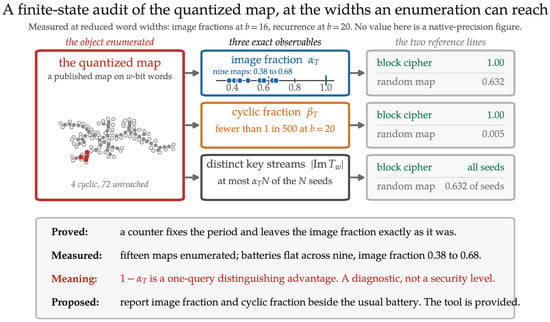
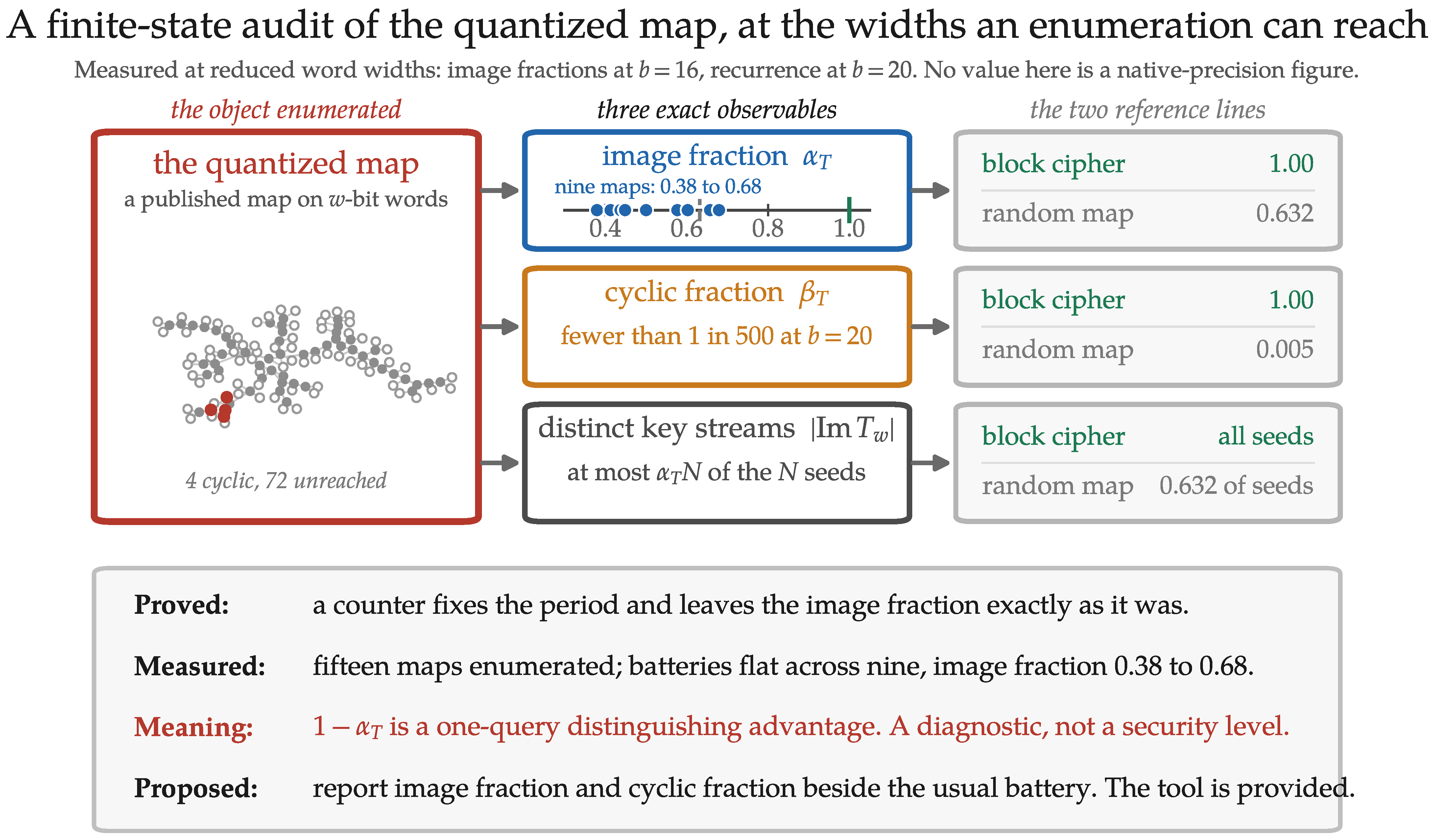

Disclaimer/Publisher’s Note: The statements, opinions and data contained in all publications are solely those of the individual author(s) and contributor(s) and not of MDPI and/or the editor(s). MDPI and/or the editor(s) disclaim responsibility for any injury to people or property resulting from any ideas, methods, instructions or products referred to in the content. |
© 2026 by the authors. Licensee MDPI, Basel, Switzerland. This article is an open access article distributed under the terms and conditions of the Creative Commons Attribution (CC BY) license.