Nonlinear Waves Passing over Rectangular Obstacles: Multimodal Method and Experimental Validation

Abstract

We report a theoretical and experimental investigation of the propagation of nonlinear waves passing over a submerged rectangular step. A multimodal method allows calculating the first- and second-order reflected and transmitted waves. In particular, at the second order, the propagation of free and bound waves is theoretically presented. A detailed analysis of the convergence of the second-order problem shows that a finite truncation of the series of evanescent bound waves is necessary to obtain a smooth and convergent solution. The computed coefficients of the first and second harmonics are experimentally validated via a complete space-time-resolved measurements of the wave propagation, which permits us to verify the relative amplitude, phase and spatial interference (beating) of the free and bound waves at the second order. This result can be useful in future multimodal models since it not only keeps the accuracy of the model with the inclusion of the first part of the evanescent bound terms (being also the dominants) but also ensures the convergence of the multimodal computation with an error that decreases as a function of the number of modes.

1. Introduction

Depth transitions are ubiquitous in coastal environments, being a crucial zone for understanding the hydrodynamics and morphology. For instance, recent investigations showed that natural hazards such as extreme waves have a place preferentially in large-depth discontinuities (Li et al. [1]). Due to widespread interest, a large variety of methods can be found in the mathematical modeling of surface water waves over variable bathymetry. In particular for the step problem, which tries to solve the wave propagation over an abrupt depth discontinuity, the scientific community’s interest has remained high due to its canonical character. Among the earliest models that solve the linear problem, we find Mei and Black [2], who developed a variational formulation, as well as Miles [3], who calculated the scattering matrix with the transmission and reflection coefficients in both directions. Moreover, the model proposed by Newman [4] considered an infinite depth before the step, which can be a reasonable simplification under certain conditions. In the same way, Boussinesq-type equations have been used in the step problem, as developed by Grue [5]. In the case of multimodal methods, the model developed by Massel [6] solves the problem of propagation of nonlinear waves over a submerged vertical step. The appeal of this model is the possibility of obtaining the reflection and transmission coefficients at the first and second order. Similarly, in the weakly nonlinear regime, more general bathymetries have been studied in Belibassakis and Athanassoulis [7] and Belibassakis and Athanassoulis [8]. Furthermore, in the linear regime, supplementary modes were proposed by Athanassoulis and Belibassakis [9], obtaining faster convergence. Moreover, oblique incident waves were considered by Rhee [10],who obtained interesting results for the phase shift of the transmitted and reflected waves. More recently, in the linear regime, Porter and Porter [11] used a conformal mapping of the fluid domain to transfer the steep deformations of the bottom topography into smooth functions applied to the modified free surface boundary conditions. More recently, some models have studied the propagation of surface wave packets (Li et al. [12]) and solitons (Ducrozet et al. [13]) over submerged steps.

In the propagation of water waves, depth transitions usually generate nonlinearities at different levels, going from weakly nonlinear waves up to breaking waves. The behavior of these nonlinear waves over submerged obstacles can be found in the theory of propagation of waves in shallow water by Massel [6] or Bryant [14]. These theories predict the evolution of waves in constant depth for different harmonics, where the second harmonic is of particular interest because of the presence of waves at different velocities. These waves are separated into free waves, which follow the dispersion relation in all the harmonics, and bound waves which are directly created by nonlinearities and are not dispersive. Thus, for a given forcing frequency $\omega$, at the n-th harmonic, the free wave has a wavenumber given by $k_n=D\left(n\omega \right)$, where D represents the linear dispersion relation of water waves. On the other side, the bound waves at the n-th harmonic has a wavenumber $n{k}_1=nD\left(\omega \right)$, being merely an integer multiple of the fundamental mode wavenumber. The mechanism of decomposition of monochromatic incident waves into free and bound waves can be found in the characterization by Huang and Dong [15]. They described the mechanism involved when the primary wave passes over the dike and generates a secondary small wave that propagates with a lower velocity than the main crest. This difference in celerity corresponds to the deviation of the dispersion relation curve with respect to the non-dispersive harmonics (bound waves). Although the presence of free and bound waves is directly observable in the $(\omega ,k)$ plane, which can be obtained from a two-dimensional Fourier transform of a space-time plane, most of the studies in nonlinear waves so far have considered punctual measurements, as carried out by Chapalain et al. [16], Beji and Battjes [17], Li and Ting [18], Benoit et al. [19] and Ohyama and Nadaoka [20]. These experimental works were mostly designed to validate numerical models by comparing temporal signals. Space-time measurements have been carried out by Brossard and Chagdali [21], Brossard et al. [22] with moving probes, where the Doppler effect permits the identification of free and bound waves in the k-spectrum. More recently, experiments performed by Li and Ting [18] and Ting et al. [23] with a vertical laser sheet measured space-time data along a channel, achieving an interesting separation of free and bound waves. However, this measurement is still in 2D, and it does not take into account the transverse effects that are always present in wave flume experiments.

In this study, we revisit a multimodal model developed by Massel [6] that gives accurate results for weakly nonlinear conditions, as verified experimentally by Ohyama et al. [24]. The numerical calculations are analyzed in terms of the convergence. We give special attention to the second order, whose source term has difficult convergence due to the abrupt depth discontinuity. Regarding the experimental validation, we report on a complete space-time-resolved measurement of nonlinear waves using Fourier Transform Profilometry (FTP) (Takeda et al. [25], Takeda and Mutoh [26]), which was adapted to surface water waves by Cobelli et al. [27]. A 3D field permits the verification of important experimental aspects such as wavefront flatness and transverse modes, making the measurements more reliable.

2. Multimodal Model

2.1. Statement of the Problem

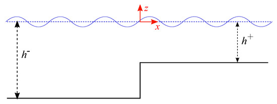
Let us consider an infinite domain in the plane $(x,z)$ where we place a depth discontinuity at $x=0$. Thus, as is shown in Figure 1, the depth $h\left(x\right)$ is the piecewise function

$$h\left(x\right)=\left\{\begin{array}{ccc}{h}^{-}\hfill & ,x<0\hfill & \\ h^{+}<h^{-}\hfill & ,x>0\hfill & ,\hfill \end{array}\right.$$

(1)

which describes a bathymetry composed of a deep water region in $x<0$ and a shallow water region in $x>0$.

Figure 1. Scheme of the propagation problem of a nonlinear wave over a submerged rectangular obstacle. The incident wave comes from the left side.

For simplicity, all the development is presented in the configuration called deep-to-shallow water, where an incident right-going wave comes from $x=-\infty$. Nevertheless, the model is perfectly applicable to the shallow-to-deep water case.

In both sides of the step, the velocity potential function $\varphi$ satisfies the Laplace equation

$$\left(\frac{{\partial }^2}{\partial x^2}+\frac{{\partial }^2}{\partial z^2}\right)\varphi =0$$

(2)

and the potential $\varphi$ and surface displacement $\eta$ satisfy the free surface kinematic boundary conditions

$$\frac{\partial \varphi }{\partial z}=\frac{\partial \eta }{\partial t}+\frac{\partial \varphi }{\partial x}\frac{\partial \eta }{\partial x},z=\eta$$

(3)

and the free surface dynamic boundary condition

$$\frac{\partial \varphi }{\partial t}+\frac{1}{2}\left[{\left(\frac{\partial \varphi }{\partial x}\right)}^2+{\left(\frac{\partial \varphi }{\partial z}\right)}^2\right]+g\eta =0,z=\eta .$$

(4)

Eventually, on the bottom and on the step wall, we impose impervious boundary conditions

$$\begin{array}{cc}\hfill \frac{\partial \varphi }{\partial z}=0,& z=-h\left(x\right)\end{array}$$

(5)

$$\begin{array}{cc}\hfill \frac{\partial \varphi }{\partial x}=0,& -h^{-}<z<-h^{+},x=0\end{array}$$

(6)

We start the solution of the problem via the perturbation method (Hsu et al. [28], Ohyama et al. [24] and Mei et al. [29]). To do so, let us consider a small parameter $ϵ$, which, in this dimensional form, corresponds to the wave amplitude a. This parameter is used in the formal expansion of the wave potential $\varphi$ and the surface displacement $\eta$

$$\begin{array}{c}\hfill \varphi (x,z,t)=ϵ{\varphi }_1(x,z,t)+{ϵ}^2{\varphi }_2(x,z,t)+\dots \end{array}$$

(7)

$$\begin{array}{c}\hfill \eta (x,t)=ϵ{\eta }_1(x,t)+{ϵ}^2{\eta }_2(x,t)+\dots \end{array}$$

(8)

Next, a Taylor series approximated the velocity potential around $z=0$ in the form

$$\varphi (x,\eta ,t)={\varphi }_{z=0}+\eta {\frac{\partial \varphi }{\partial z}}_{z=0}+\frac{1}{2}{\eta }^2{\frac{{\partial }^2\varphi }{\partial z^2}}_{z=0}+\dots$$

(9)

The power expansion of Equations (7) and (8) and the Taylor series of Equation (9) are replaced in the Laplace Equation (2) and in the free surface and bottom boundary conditions (Equations (3) to (6)). Then, we truncate the expressions at the order $ϵ$ to obtain the first-order system with a Laplace Equation that reads

$$\left(\frac{{\partial }^2}{\partial x^2}+\frac{{\partial }^2}{\partial z^2}\right){\varphi }_1=0$$

(10)

with the boundary conditions at the free surface

$$\frac{{\partial }^2{\varphi }_1}{\partial t^2}+g\frac{\partial {\varphi }_1}{\partial z}=0,z=0,$$

(11)

and

$$g{\eta }_1+\frac{\partial {\varphi }_1}{\partial t}=0,z=0,$$

(12)

and the impervious bottom boundary conditions

$$\frac{\partial {\varphi }_1}{\partial z}=0,z=-h,$$

(13)

and

$$\frac{\partial {\varphi }_1}{\partial x}=0,-h^{-}<z<-h^{+},x=0.$$

(14)

We state the diffraction problem of water waves by setting at infinity, in $x<0$, that there are one incident wave and one reflected wave from the discontinuity. On the other hand, at the positive infinity in $x>0$, there is only one transmitted wave (outgoing wave). Eventually, at the depth transition, the potential $\varphi$ and its spatial derivative are continuous in the whole domain, that is, $\left[\varphi \right]=0$ and $\left[\frac{\partial }{\partial x}\varphi \right]=0$, at $x=0$ and at $-h^{+}<z<0$.

Solution of First Order

We define the space-time-dependent functions corresponding to the incident and reflected waves as

$$I_0^{\left(1\right)}(x,t)=\frac{ga}{\omega }{e}^{i(k_0^{-}x-\omega t)},x<0,$$

(15)

$$A_n^{\left(1\right)}(x,t)=\frac{ga}{\omega }{e}^{-i(k_n^{-}x+\omega t)},x<0,$$

(16)

$$B_m^{\left(1\right)}(x,t)=\frac{ga}{\omega }{e}^{i(k_m^{+}x-\omega t)},x>0,$$

(17)

where $k_0^{\pm }$ corresponds to the unique real propagating solution and $k_n^{\pm }=i{k}_1^{\pm },i{k}_2^{\pm },i{k}_3^{\pm },\dots$ to the infinite imaginary evanescent solutions of the dispersion relation of surface gravity waves

$${\omega }^2=g{k}_n^{\pm }tanh\left(k_n^{\pm }{h}^{\pm }\right).$$

(18)

Here, in Equations (16) and (17) and in what follows, for the sake of clarity, we shall use the variable $n=0,1,2,3,\dots$ as the index of the functions in the deep water region ($x<0$, $h^{-}$) and the variable $m=0,1,2,3,\dots$ as the index of the functions in the shallow water region ($x>0$, $h^{+}$). In addition, the orthogonal basis function that satisfies the boundary conditions (11) to (13) is a z-dependent function in the form

$$F_n^{\left(1\right)}\left(z\right)=\frac{cosh{k}_n^{-}(z+h^{-})}{cosh{k}_n^{-}{h}^{-}},x<0,$$

(19)

$$G_m^{\left(1\right)}\left(z\right)=\frac{cosh{k}_m^{+}(z+h^{+})}{cosh{k}_m^{+}{h}^{+}},x>0.$$

(20)

Hence, the linear potential for both deep and shallow water regions can be written as

$${\varphi }_1^{-}=I_0^{\left(1\right)}{F}_0^{\left(1\right)}+\sum _n{R}_n^{\left(1\right)}{A}_n^{\left(1\right)}{F}_n^{\left(1\right)},x<0,$$

(21)

$${\varphi }_1^{+}=\sum _m{T}_m^{\left(1\right)}{B}_m^{\left(1\right)}{G}_m^{\left(1\right)},x>0,$$

(22)

where $R_n^{\left(1\right)}$ and $T_m^{\left(1\right)}$ are the unknown reflection and transmission coefficients of the first-order problem. From the continuity conditions at $x=0$ for the potential $\varphi$ and its spatial derivative, we obtain the following equations

$$\begin{array}{c}\hfill {\left.{\varphi }_1^{-}\right|}_{x=0^{-}}={\left.{\varphi }_1^{+}\right|}_{x=0^{+}}\end{array}$$

(23)

$$\begin{array}{c}\hfill {\left.\frac{\partial {\varphi }_1^{-}}{\partial x}\right|}_{x=0^{-}}={\left.\frac{\partial {\varphi }_1^{+}}{\partial x}\right|}_{x=0^{+}}.\end{array}$$

(24)

For faster convergence, we consider a number of modes $N^{-}$ for the deep water region and $N^{+}\approx \left(h^{+}/h^{-}\right)N^{-}$ for the shallow water region. By replacing Equations (21) and (22) in the conditions (23) and (24), we obtain

$$I_0^{\left(1\right)}{F}_0^{\left(1\right)}+\sum _n{R}_n^{\left(1\right)}{A}_n^{\left(1\right)}{F}_n^{\left(1\right)}=\sum _m{T}_m^{\left(1\right)}{B}_m^{\left(1\right)}{G}_m^{\left(1\right)},$$

(25)

$${\partial }_x{I}_0^{\left(1\right)}{F}_0^{\left(1\right)}+\sum _n{R}_n^{\left(1\right)}{\partial }_x{A}_n^{\left(1\right)}{F}_n^{\left(1\right)}=\sum _m{T}_m^{\left(1\right)}{\partial }_x{B}_m^{\left(1\right)}{G}_m^{\left(1\right)}.$$

(26)

Next, we project Equation (25) onto the orthogonal basis $G_m^{\left(1\right)}$

$$I_0^{\left(1\right)}{\int }_{-h^{+}}^0{F}_0^{\left(1\right)}{G}_m^{\left(1\right)}+\sum _n{R}_n^{\left(1\right)}{A}_n^{\left(1\right)}{\int }_{-h^{+}}^0{F}_n^{\left(1\right)}{G}_m^{\left(1\right)}=T_m^{\left(1\right)}{B}_m^{\left(1\right)}{\int }_{-h^{+}}^0{\left(G_m^{\left(1\right)}\right)}^2,$$

(27)

where we have used the orthogonality of the basis $G_m^{\left(1\right)}$ to eliminate the sum in m on the right-hand side, i.e., Equation (27) is written for each m with $0\le m\le (N^{+}-1)$. Before projecting Equation (26), we use the boundary condition from Equation (14) to impose the following equivalence of the integrals of the derivative

$${\int }_{-h^{-}}^0\frac{\partial {\varphi }_1}{\partial x}{F}_n^{\left(1\right)}dz={\int }_{-h^{+}}^0\frac{\partial {\varphi }_1}{\partial x}{F}_n^{\left(1\right)}dz,x=0,$$

(28)

which we use to project Equation (26) onto the orthogonal basis $F_n^{\left(1\right)}$, and obtain

$${\partial }_x{I}_0^{\left(1\right)}{\int }_{-h^{-}}^0{F}_0^{\left(1\right)}{F}_n^{\left(1\right)}+R_n^{\left(1\right)}{\partial }_x{A}_n^{\left(1\right)}{\int }_{-h^{-}}^0{\left(F_n^{\left(1\right)}\right)}^2=\sum _m{T}_m^{\left(1\right)}{\partial }_x{B}_m^{\left(1\right)}{\int }_{-h^{+}}^0{F}_n^{\left(1\right)}{G}_m^{\left(1\right)},$$

(29)

where we have used the orthogonality of the basis $F_n^{\left(1\right)}$ to eliminate the sum in n on the left-hand side, i.e., Equation (29) is written for each n with $0\le n\le (N^{-}-1)$. Therefore, we obtain $N^{-}+N^{+}$ projected equations.

Eventually, the system of Equations (27) and (29) can be solved for $R_n^{\left(1\right)}$, as is detailed in Appendix A.1, and then the transmission coefficients $T_m^{\left(1\right)}$ can be easily obtained from Equation (27).

2.2. Second Order Problem

2.2.1. Statement of the Problem

Now after replacing Equations (7) to (9) in the system of Equation (5) to (2) to (4), we keep the terms at the order ${ϵ}^2$. This leads to the nonlinear wave problem at second order where the solution ${\varphi }_2$ should satisfy the Laplace equation

$$\left(\frac{{\partial }^2}{\partial x^2}+\frac{{\partial }^2}{\partial z^2}\right){\varphi }_2=0$$

(30)

with the following boundary conditions at the free surface

$$\begin{array}{c}\hfill \frac{{\partial }^2{\varphi }_2}{\partial t^2}+g\frac{\partial {\varphi }_2}{\partial z}=-\frac{\partial }{\partial t}\left[{\left(\frac{\partial {\varphi }_1}{\partial x}\right)}^2+{\left(\frac{\partial {\varphi }_1}{\partial z}\right)}^2\right]-{\eta }_1\frac{\partial }{\partial z}\left[\frac{{\partial }^2{\varphi }_1}{\partial t^2}+g\frac{\partial {\varphi }_1}{\partial z}\right],z=0,\end{array}$$

(31)

$$\begin{array}{c}\hfill g{\eta }_2+\frac{\partial {\varphi }_2}{\partial t}=-\frac{1}{2}\left[{\left(\frac{\partial {\varphi }_1}{\partial x}\right)}^2+{\left(\frac{\partial {\varphi }_1}{\partial z}\right)}^2\right]-{\eta }_1\frac{{\partial }^2{\varphi }_1}{\partial z\partial t},z=0,\end{array}$$

(32)

and impervious boundary conditions at the bottom

$$\frac{\partial {\varphi }_2}{\partial z}=0,z=-h\left(x\right),$$

(33)

$$\frac{\partial {\varphi }_2}{\partial x}=0,-h^{-}<z<-h^{+},x=0.$$

(34)

This represents a non-homogeneous surface wave equation. Considering that the non-homogeneous wave problem has one particular and one homogeneous solution (${\varphi }_2={\varphi }_2^b+{\varphi }_2^f$), we can state the boundary conditions separately at $x=\pm \infty$. First, the right side of Equation (31) depends on ${\varphi }_1$, which implies that the particular solution (${\varphi }_2^b$) has the same boundary conditions as for ${\varphi }_1$. Thus, we have at the negative infinity, in $x<0$, there are one incident wave and one reflected wave, and at the positive infinity, in $x>0$, there is only one transmitted outgoing wave. Moreover, because the homogeneous second-order problem does not consider a source term with energy coming from the infinity, we have the Sommerfeld radiation condition (Sommerfeld [30]), which only considers outgoing waves in both sides of the domain; it is $x=\pm \infty$. Similarly to the first-order problem, the second-order problem should satisfy the continuity of the potential and its spatial derivative. Thus, we have jump conditions as $\left[{\varphi }_2\right]=0$ and $\left[\frac{\partial }{\partial x}{\varphi }_2\right]=0$ at $x=0$ and at $-h^{+}<z<0$.

2.2.2. Second-Order Particular Solution

The kinematic and dynamic boundary conditions expressed in Equations (31) and (32) have a source term depending on the solution of the linear problem. The solution of this equation is composed by one particular solution ${\varphi }_2^b$ (bound wave) and one homogeneous solution ${\varphi }_2^f$ (free wave). Thus, the complete solution is

$${\varphi }_2={\varphi }_2^b+{\varphi }_2^f.$$

(35)

We start by finding the bound wave terms, which depend on ${\varphi }_1$. We can find and write the incident second-order potential in terms of the following $(x,t)$ and z-dependent functions

$$I_{0,0}^{(1,1)}(x,t)=C_{0,0}^{(1,1)}{e}^{2i{k}_0^{-}x-2i\omega t}+c.c.$$

(36)

$$F_{0,0}^{(1,1)}\left(z\right)=\frac{cosh2k_0^{-}(z+h^{-})}{cosh2k_0^{-}{h}^{-}}$$

(37)

where $C_{0,0}^{(1,1)}$ is the constant of the second-order propagating bound wave (as in Equation (36), we shall use in what follows the super-index ${\left(\right)}^{(1,1)}$ to indicate the constants and functions resulting from replacing the solution of the first-order ${\varphi }_1$ and ${\eta }_1$ in the right side of Equations (31) and (32)). This second-order wave, usually called Stokes harmonic, is the solution of Equation (31) when there is only one incident wave (Equation (15)). Thus, it always exists in the propagation of a single wave in constant depth. The simplified expression of the Stokes harmonic is

$$I_{0,0}^{(1,1)}(x,t)F_{0,0}^{(1,1)}\left(z\right)=\frac{3}{8}\frac{\omega a^{2}cosh2k_0^{-}(z+h^{-})}{{sinh}^4\left(k_0^{-}{h}^{-}\right)}{e}^{2i{k}_0^{-}x-2i\omega t}+c.c.$$

(38)

Likewise, the bound reflected waves can be written in terms of the $(x,t)$-dependent function

$$A_{n,n^{\prime }}^{(1,1)}(x,t)=C_{n,n^{\prime }}^{(1,1)}{e}^{-i(k_n^{-}+k_{n^{\prime }}^{-})x-2i\omega t}+c.c.$$

(39)

where the constant $C_{n,n^{\prime }}^{(1,1)}$ is the bound waves’ constant depending on the linear reflection coefficients and is detailed in the Appendix B.2.

For the shallow water region, the bound waves depend on the transmitted linear wave and are obtained by replacing Equation (22) in the right-hand side of Equation (31). Thus, the $(x,t)$-dependent function, in $x>0$, can be expressed as

$$B_{m,m^{\prime }}^{(1,1)}(x,t)=C_{m,m^{\prime }}^{(1,1)}{e}^{i(k_m^{+}+k_{m^{\prime }}^{+})x-2i\omega t}+c.c.$$

(40)

where the coefficient $C_{m,m^{\prime }}^{(1,1)}$ has the same form as Equation (A5) but uses wavenumbers and depth from the shallow water region ($k_m^{+}$, $h^{+}$). In order to satisfy the source term of Equations (31) and (32), the z dependency in the bound waves is expressed in the following form

$$F_{n,n^{\prime }}^{(1,1)}\left(z\right)=\frac{cosh(k_n^{-}+k_{n^{\prime }}^{-})(z+h^{-})}{cosh(k_n^{-}+k_{n^{\prime }}^{-})h^{-}},x<0,$$

(41)

$$G_{m,m^{\prime }}^{(1,1)}\left(z\right)=\frac{cosh(k_m^{+}+k_{m^{\prime }}^{+})(z+h^{+})}{cosh(k_m^{+}+k_{m^{\prime }}^{+})h^{+}},x>0.$$

(42)

In addition, the second-order evanescent terms resulting from the multiplication of the Stokes incident harmonic with the evanescent reflected bound waves can be expressed as

$$D_{0,n}^{(1,1)}\left(x\right)=C_{0,n}^{(1,1)}{e}^{(i{k}_0^{-}-k_n^{-})x-2i\omega t}+c.c.$$

(43)

where the constant coefficient $C_{0,n}^{(1,1)}$ is detailed in Appendix B.2. The z-dependent function corresponds to

$$H_{0,n}^{(1,1)}\left(z\right)=\frac{cosh(k_0^{-}-k_n^{-})(z+h^{-})}{cosh(k_0^{-}-k_n^{-})h^{-}},x<0.$$

(44)

Eventually, the second-order bound wave potential is

$${\varphi }_2^{b-}=I_{0,0}^{(1,1)}{F}_{0,0}^{(1,1)}+\sum _n\sum _{n^{\prime }}{R}_n^{\left(1\right)}{R}_{n^{\prime }}^{\left(1\right)}{A}_{n,n^{\prime }}^{(1,1)}{F}_{n,n^{\prime }}^{(1,1)}+\sum _n{R}_n^{\left(1\right)}{D}_{0,n}^{(1,1)}{H}_{0,n}^{(1,1)}+c.c.,x<0,$$

(45)

$${\varphi }_2^{b+}=\sum _m\sum _{m^{\prime }}{T}_m^{\left(1\right)}{T}_{m^{\prime }}^{\left(1\right)}{B}_{m,m^{\prime }}^{(1,1)}{G}_{m,m^{\prime }}^{(1,1)}+c.c.,x>0.$$

(46)

2.2.3. Second-Order Homogeneous Solution

In order to satisfy the homogeneous solution (without source terms from ${\varphi }_1$), the free waves should follow the dispersion relation at the frequency $2\omega$. Thus, second-order dispersive terms are generated only at depth inhomogeneity due to the absence of dispersive terms in the incident wave. As a consequence, the Sommerfeld radiation condition is imposed to the free waves, which implies that the $(x,t)$-dependent functions have the following form

$$A_p^{\left(2\right)}(x,t)=\frac{ga}{2\omega }{e}^{-i({\kappa }_p^{-}x+2\omega t)}+c.c.,x<0$$

(47)

$$B_q^{\left(2\right)}(x,t)=\frac{ga}{2\omega }{e}^{i({\kappa }_q^{+}x-2\omega t)}+c.c.,x>0$$

(48)

where ${\kappa }_p^{\pm }={\kappa }_0^{\pm },i{\kappa }_1^{\pm },i{\kappa }_2^{\pm },i{\kappa }_3^{\pm },\dots$ correspond to the unique real solution $(p=0)$ and to the infinite imaginary solutions $(p=1,2,\dots ,N^{-})$ of the dispersion relation

$${\left(2\omega \right)}^2=g{\kappa }_p^{\pm }tanh\left({\kappa }_p^{\pm }{h}^{\pm }\right)$$

(49)

For the sake of clarity, we shall use, as in Equations (47) and (48), the sub-index p to identify the constants and functions of the second-order homogeneous solution in the deep water region ($x<0$, $h^{-}$) and the sub-index q to identify the constants and functions of the second-order homogeneous solution in the shallow water region ($x>0$, $h^{+}$).

The orthogonal basis of z-dependent functions that satisfy the boundary conditions (31) to (34) is expressed in the same way as for the linear problem

$$F_p^{\left(2\right)}\left(z\right)=\frac{cosh{\kappa }_p^{-}(z+h^{-})}{cosh{\kappa }_p^{-}{h}^{-}},x<0,$$

(50)

$$G_q^{\left(2\right)}\left(z\right)=\frac{cosh{\kappa }_q^{+}(z+h^{+})}{cosh{\kappa }_q^{+}{h}^{+}},x>0.$$

(51)

Next, the free wave potential at the second order corresponds to the following sum

$${\varphi }_2^{f-}=\sum _p{R}_p^{\left(2\right)}{A}_p^{\left(2\right)}{F}_p^{\left(2\right)}+c.c.,x<0$$

(52)

$${\varphi }_2^{f+}=\sum _q{T}_q^{\left(2\right)}{B}_q^{\left(2\right)}{G}_q^{\left(2\right)}+c.c.,x>0$$

(53)

where the unknowns $R_p^{\left(2\right)}$ and $T_q^{\left(2\right)}$ are the transmission and reflection coefficients that shall be obtained in the next calculation.

2.2.4. Construction of the Complete Second-Order Solution

Similarly to the linear problem, we impose the continuity of the second-order potential and its derivative at the step position. Thus, we have

$$\left[{\varphi }_2\right]=0,x=0,$$

(54)

$$\left[{\partial }_x{\varphi }_2\right]=0,x=0,$$

(55)

which means that the free and bound wave potential should satisfy

$${\varphi }_2^{b-}+{\varphi }_2^{f-}={\varphi }_2^{b+}+{\varphi }_2^{f+},$$

(56)

$${\partial }_x{\varphi }_2^{b-}+{\partial }_x{\varphi }_2^{f-}={\partial }_x{\varphi }_2^{b+}+{\partial }_x{\varphi }_2^{f+},$$

(57)

which is the set of equations of the unknowns $R_p^{\left(2\right)}$ and $T_q^{\left(2\right)}$.

Next, we project Equation (56) onto the orthogonal basis $G_q^{\left(2\right)}$, which yields

$$\begin{array}{c}\hfill I_{0,0}^{(1,1)}{\int }_{-h^{+}}^0{F}_{0,0}^{(1,1)}{G}_q^{\left(2\right)}+{\displaystyle \sum _n}{\displaystyle \sum _{n^{\prime }}}{R}_n^{\left(1\right)}{R}_{n^{\prime }}^{\left(1\right)}{A}_{n,n^{\prime }}^{(1,1)}{\int }_{-h^{+}}^0{F}_{n,n^{\prime }}^{(1,1)}{G}_q^{\left(2\right)}+{\displaystyle \sum _n}{R}_n^{\left(1\right)}{D}_{0,n}^{(1,1)}{\int }_{-h^{+}}^0{H}_{0,n}^{(1,1)}{G}_q^{\left(2\right)}+\\ \hfill {\displaystyle \sum _p}{R}_p^{\left(2\right)}{A}_p^{\left(2\right)}{\int }_{-h^{+}}^0{F}_p^{\left(2\right)}{G}_q^{\left(2\right)}+c.c.={\displaystyle \sum _m}{\displaystyle \sum _{m^{\prime }}}{T}_m^{\left(1\right)}{T}_{m^{\prime }}^{\left(1\right)}{B}_{m,m^{\prime }}^{(1,1)}{\int }_{-h^{+}}^0{G}_{m,m^{\prime }}^{(1,1)}{G}_q^{\left(2\right)}+T_q^{\left(2\right)}{B}_q^{\left(2\right)}{\int }_{-h^{+}}^0{\left(G_q^{\left(2\right)}\right)}^2+c.c.\end{array}$$

(58)

where we have used the orthogonality of the basis $G_q^{\left(2\right)}$ to eliminate the sum in q in the right-hand side of the equation, i.e., the projected Equation (58) is written for each q-th term.

Before projecting Equation (57), we use the boundary condition from Equation (34) to impose the following equivalence of the integrals of the derivative

$${\int }_{-h^{-}}^0\frac{\partial {\varphi }_2}{\partial x}dz={\int }_{-h^{+}}^0\frac{\partial {\varphi }_2}{\partial x}dz,x=0,$$

(59)

which is used to project Equation (57) onto the orthogonal basis $F_p^{\left(2\right)}$ and to obtain

$$\begin{array}{c}\hfill {\partial }_x{I}_{0,0}^{(1,1)}{\int }_{-h^{-}}^0{F}_{0,0}^{(1,1)}{F}_p^{\left(2\right)}+{\displaystyle \sum _n}{\displaystyle \sum _{n^{\prime }}}{R}_n^{\left(1\right)}{R}_{n^{\prime }}^{\left(1\right)}{\partial }_x{A}_{n,n^{\prime }}^{(1,1)}{\int }_{-h^{-}}^0{F}_{n,n^{\prime }}^{(1,1)}{F}_p^{\left(2\right)}+{\displaystyle \sum _n}{R}_n^{\left(1\right)}{\partial }_x{D}_{0,n}^{(1,1)}{\int }_{-h^{-}}^0{H}_{0,n}^{(1,1)}{F}_p^{\left(2\right)}+\\ \hfill R_p^{\left(2\right)}{\partial }_x{A}_p^{\left(2\right)}{\int }_{-h^{-}}^0{\left(F_p^{\left(2\right)}\right)}^2+c.c.={\displaystyle \sum _m}{\displaystyle \sum _{m^{\prime }}}{T}_m^{\left(1\right)}{T}_{m^{\prime }}^{\left(1\right)}{\partial }_x{B}_{m,m^{\prime }}^{(1,1)}{\int }_{-h^{+}}^0{G}_{m,m^{\prime }}^{(1,1)}{F}_p^{\left(2\right)}+{\displaystyle \sum _q}{T}_q^{\left(2\right)}{\partial }_x{B}_q^{\left(2\right)}{\int }_{-h^{+}}^0{G}_q^{\left(2\right)}{F}_p^{\left(2\right)}+c.c.,\end{array}$$

(60)

Here, we have used the orthogonality of the basis $F_p^{\left(2\right)}$ to eliminate the sum in p in the left-hand side of the equation, i.e., the projected Equation (60) is written for each p-th term.

Finally, the system of Equations (58) and (60) can be solved for $R_p^{\left(2\right)}$, as is detailed in Appendix B.2, and then the transmission coefficients $T_q^{\left(2\right)}$ can be easily obtained from Equation (58).

3. Numerical Calculation

3.1. Solution of the First-Order Problem

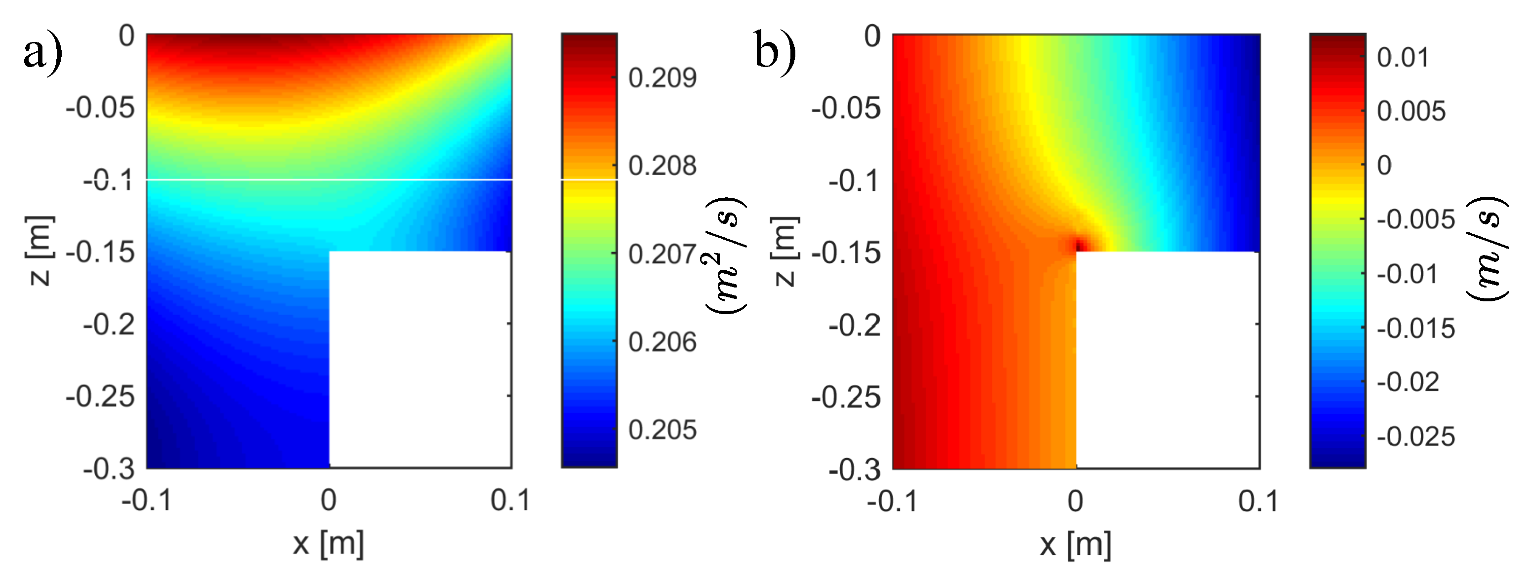
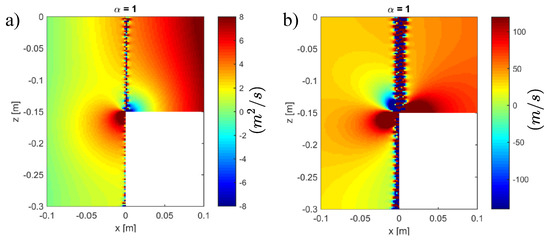
We show in this section a numerical implementation of the first-order system of Equation (A1). This numerical example has been built with the parameters $a=0.023$ m, $h^{-}=0.3$ m, $h^{+}=0.15$ m and $\omega =2\pi$ ${\mathrm{s}}^{-1}$. In Figure 2, we present the near field of the velocity potential ${\varphi }_1$ as well as the horizontal velocity ${\partial }_x{\varphi }_1$ calculated for $N^{-}=64$ modes. As we observe, the first-order problem, considering it is homogeneous and linear, has a robust convergence with a smooth solution that is independent of the wave amplitude and frequency.

Figure 2. (a) Velocity potential at the first-order ${\varphi }_1$ near the step. (b) Horizontal velocity at the first-order ${\partial }_x{\varphi }_1$ near the step.

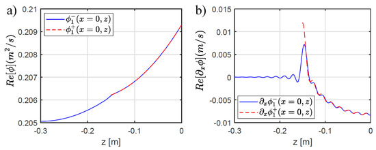
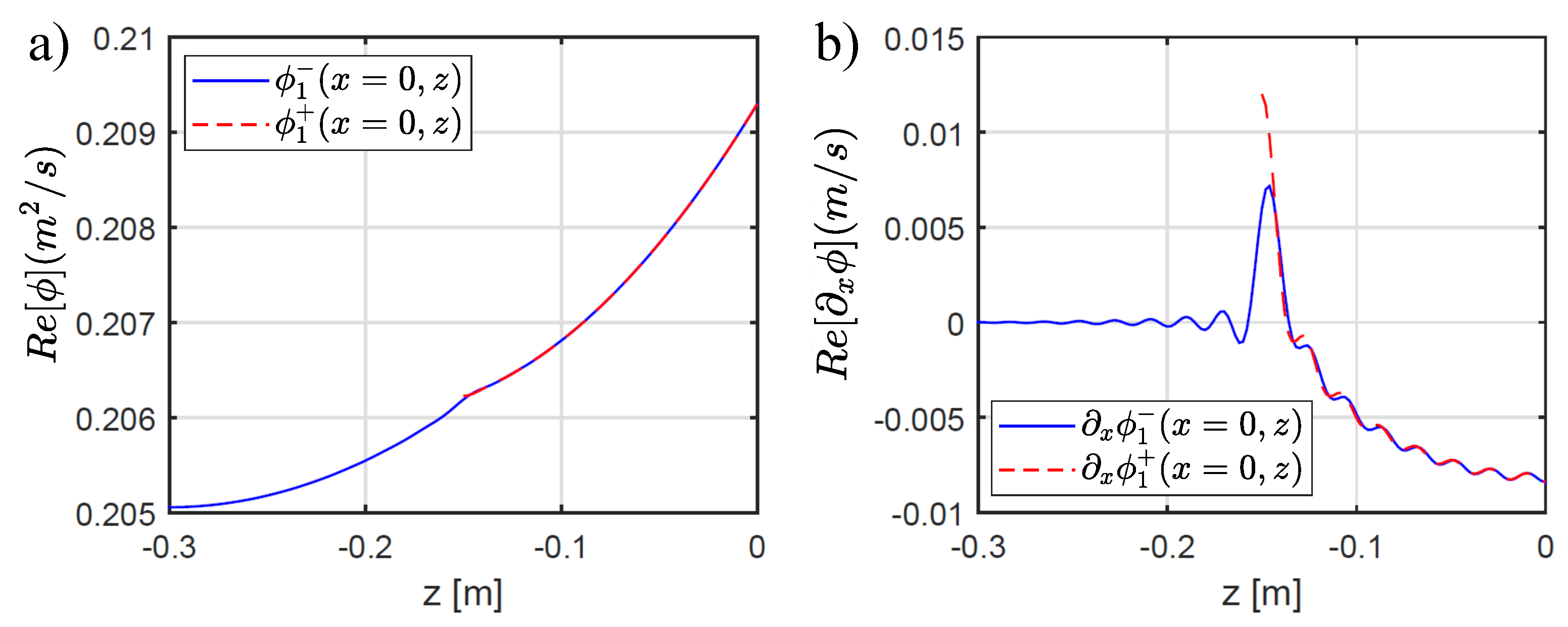
In Figure 2b, in the neighborhood of the corner, at $(x=0,z=-0.15)$ m, we observe a local divergence of the horizontal velocity, which is the classical behavior of a potential flow around a tip. In more detail, the profile of the matching of the potential and horizontal velocity is presented in Figure 3. The real part of the functions ${\varphi }_1^{-}(x=0,z)$ and ${\varphi }_1^{+}(x=0,z)$ are plotted in Figure 3a, where a very good agreement is observed in the vertical range $0.15<z<0$ m. On the other hand, in Figure 3b, we present the vertical profile of the match of the horizontal velocity, that is, ${\partial }_x{\varphi }_1^{-}(x=0,z)$ and ${\partial }_x{\varphi }_1^{+}(x=0,z)$. As expected, the divergence of the velocity around the corner is difficult to match in this part, showing nevertheless a good match in the rest of the domain. The boundary condition of the impervious wall at the step in Equation (14) is also well satisfied by the function ${\partial }_x{\varphi }_1^{-}(x=0,z)$ in the range $-0.3<z<-0.15$ m, especially far from the rectangular corner. This match, as shall be shown further on, is improved as a function of the number of modes $(N^{-},N^{+})$.

Figure 3. (a) Vertical profile at $x=0$ of the velocity potential at the first-order ${\varphi }_1$. (b) Vertical profile at $x=0$ of the horizontal velocity at the first-order ${\partial }_x{\varphi }_1$.

3.2. Solution of the Second-Order Problem

In the second-order problem, the presence of a source term in the right-hand side of Equations (31) and (32) can lead to convergence problems. The first natural trial is the solution of the second order considering all the terms obtained from the first-order solution, i.e., making the limits of the double and single sums in Equations (45) and (46) up to $n=N^{-}$ and $m=N^{+}$. The first term of these sums correspond to a propagating wave, whereas the following terms correspond to evanescent bound waves. Therefore, by injecting the first-order solution shown in Figure 2 in the source term of Equations (31) and (32) and solving the system of Equation (A7), we obtain a solution ${\varphi }_2$ and ${\partial }_x{\varphi }_2$, as shown in Figure 4a,b, that is not smooth and has a clear divergence in the matching zone. This divergence, observed when the evanescent bound waves are included in the source term, has been recently reported by Li et al. [12], where, due to convergence problems, the contribution of bound evanescent waves was not considered.

Figure 4. Non-convergent solution of the second-order problem, $\alpha =1$ (without truncation of forcing evanescent waves). (a) Velocity potential at the second-order ${\varphi }_2$ near the step. (b) Horizontal velocity at the second-order ${\partial }_x{\varphi }_2$ near the step.

Although the first-order problem has a good convergence, the second order shows problems when we increase the number of evanescent modes in the total bound wave, which is the result of the sum of all the evanescent modes obtained from Equations (A5) and (A6). The second order solves the problem of finding the proper free wave that compensates for the bound wave field in order to obtain a smooth solution (satisfying the matching conditions). To do so, the bound wave field should have a limited amplitude, i.e., it should not grow as a function of the number of modes.

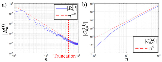
In this analysis, we focus on $n=n^{\prime }$, which is the fastest growth in the double sum of Equation (45). Thus, we consider the term ${\left(R_n^{\left(1\right)}\right)}^2{C}_{n,n}^{(1,1)}$. In Figure 5a, we show the decay of the first-order reflection coefficient and the slope $n^{-2}$ for comparison. We observe that for the case of $N^{-}=100$, the decay is slower than $n^{-2}$ for $n>50$ approximately. In contrast, as we observe in Figure 5b, the bound wave coefficient $|C_{n,n}^{(1,1)}|$ has growth at the power $n^4$. Therefore, the decay of the first-order coefficients ($R_n^{\left(1\right)}$, $T_m^{\left(1\right)}$) does not compensate for the growth of the bound evanescent wave constants, and some modification should be carried out to ensure the convergence of the second-order problem.

Figure 5. (a) Reflection coefficient $R_n^{\left(1\right)}$ of the first order for $N^{-}=100$ modes. (b) Evanescent forcing coefficients $C_{n,n}^{(1,1)}$ at the second order for $N^{-}=100$ modes.

From the observation of the decay of Figure 5a, we have that the exponent of the decay decreases close to the end of the series. This suggests that a compensation of the growth of the coefficients $C_{n,n}^{(1,1)}$ can be possible if we consider only part of the series $R_n^{\left(1\right)}$, especially the first part that has faster decay. Therefore, we propose a truncation of the evanescent waves terms into the bound wave solution. To do so, we rewrite Equations (45) and (46) as

$${\varphi }_2^{b-}=I_{0,0}^{(1,1)}{F}_{0,0}^{(1,1)}+\sum _{n=0}^{\alpha N^{-}}\sum _{n^{\prime }=0}^{\alpha N^{-}}{R}_n^{\left(1\right)}{R}_{n^{\prime }}^{\left(1\right)}{A}_{n,n^{\prime }}^{(1,1)}{F}_{n,n^{\prime }}^{(1,1)}+\sum _{n=0}^{\alpha N^{-}}{R}_n^{\left(1\right)}{D}_{0,n}^{(1,1)}{H}_{0,n}^{(1,1)}+c.c.,x<0$$

(61)

$${\varphi }_2^{b+}=\sum _{m=0}^{\alpha N^{+}}\sum _{m^{\prime }=0}^{\alpha N^{+}}{T}_m^{\left(1\right)}{T}_{m^{\prime }}^{\left(1\right)}{B}_{m,m^{\prime }}^{(1,1)}{G}_{m,m^{\prime }}^{(1,1)}+c.c.,x>0$$

(62)

where $\alpha$ is an arbitrary truncation coefficient in the range $0<\alpha \le 1$.

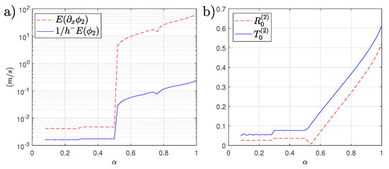
A systematic exploration of the convergence of the second-order solution as a function of $\alpha$ is shown in Figure 6a,b. The numerical error of the multimodal matching is calculated for the potential ${\varphi }_2$ as

$$E\left({\varphi }_2\right)={\int }_{-h^{+}}^0|{\varphi }_2^{+}(x=0,z)-{\varphi }_2^{-}(x=0,z)|dz,$$

(63)

and for the horizontal velocity ${\partial }_x{\varphi }_2$ as

$$E\left({\partial }_x{\varphi }_2\right)={\int }_{-h^{+}}^0|{\partial }_x{\varphi }_2^{+}(x=0,z)-{\partial }_x{\varphi }_2^{-}(x=0,z)|dz,$$

(64)

and is plotted in Figure 6a as a function of $\alpha$, where we observe an abrupt increase in $E\left({\varphi }_2\right)$ and $E\left({\partial }_x{\varphi }_2\right)$ at $\alpha >0.5$. For this calculation, we have considered $N^{-}=100$ and $N^{+}=50$ modes and increased the truncation coefficient $\alpha$ progressively. Likewise, we have verified the evolution of the propagating coefficients at the second order. As we observe in Figure 6b, the coefficients $R_0^{\left(2\right)}$ and $T_0^{\left(2\right)}$ show a stable behavior up to the limit $\alpha =0.5$, beyond which the coefficients diverge and change rapidly as a function of $\alpha$. This threshold, after several numerical calculations, seems to be independent of input parameters, such as geometry, wave amplitude and frequency. Therefore, we consider in what follows that the truncation coefficient $\alpha =0.5$ ensures the convergence of the second-order solution.

Figure 6. (a) Numerical error of the multimodal matching for the second-order functions ${\varphi }_2$ and ${\partial }_x{\varphi }_2$ as a function of the truncation parameter $\alpha$. (b) Reflection and transmission coefficients of the free waves at the second order as a function of the truncation parameter $\alpha$.

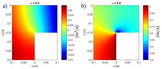
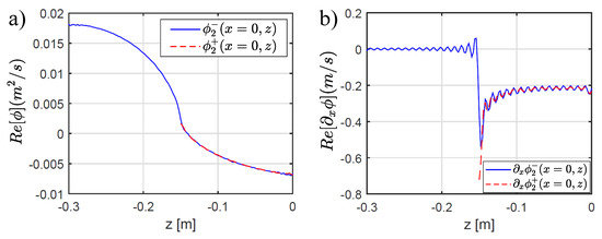
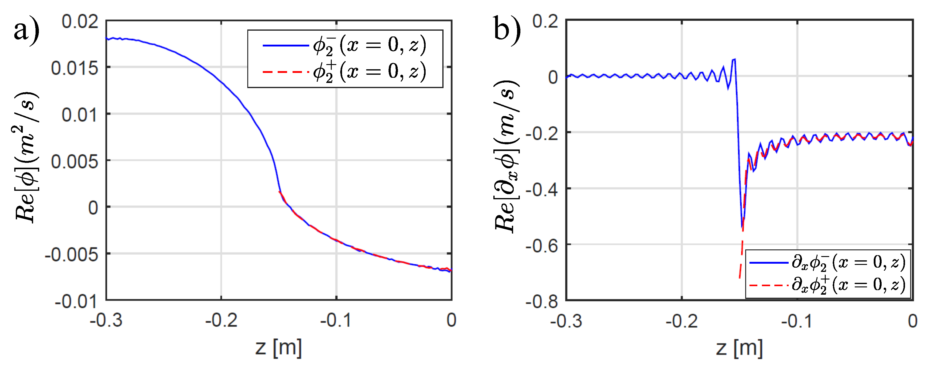
A numerical example calculated with $N^{-}=64$, $N^{+}=32$ modes and $\alpha =0.5$ is presented in Figure 7a,b, for the near field of ${\varphi }_2$ and ${\partial }_x{\varphi }_2$, respectively. Both fields, at the depth discontinuity, show a smooth transition between the deep and shallow water regions, confirming the convergence of the solution. The agreement of the multimodal matching can be verified more in detail in the vertical profile shown in Figure 8a,b, where an excellent match between the potential ${\varphi }_2$ and the velocity ${\partial }_x{\varphi }_2$ at both sides of the step confirms the accuracy of the multimodal matching after applying the truncation method.

Figure 7. Convergent solution of the second-order problem for $\alpha =0.5$ (with truncation of forcing evanescent waves). (a) Velocity potential ${\varphi }_2$ at the second order near the step. (b) Horizontal velocity ${\partial }_x{\varphi }_2$ at the second order near the step.

Figure 8. (a) Vertical profile at $x=0$ of the velocity potential at the second order ${\varphi }_2(0,z)$. (b) Vertical profile at $x=0$ of the horizontal velocity at the first-order ${\partial }_x{\varphi }_2(0,z)$.

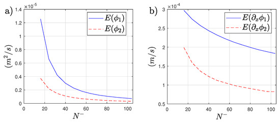
Eventually, we show in Figure 9 the numerical error calculated in Equations (63) and (64) for the case $\alpha =0.5$. In Figure 9a, we show the numerical error of the velocity potential for the first- and second-order problems, which are in both cases decaying. Similarly, in Figure 9b, the numerical error of the horizontal velocities at the first and second order also decay monotonically as a function of the number of modes.

Figure 9. Numerical error of the multimodal matching as a function of the number of modes for the case $\alpha =0.5$. (a) Numerical error of the velocity potentials ${\varphi }_1$ and ${\varphi }_2$. (b) Numerical error of the horizontal velocities ${\partial }_x{\varphi }_1$ and ${\partial }_x{\varphi }_2$.

4. Experimental Measurements

4.1. Experimental Set-Up

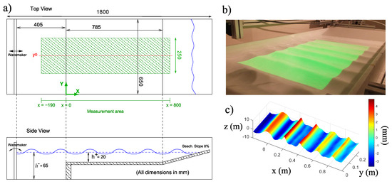
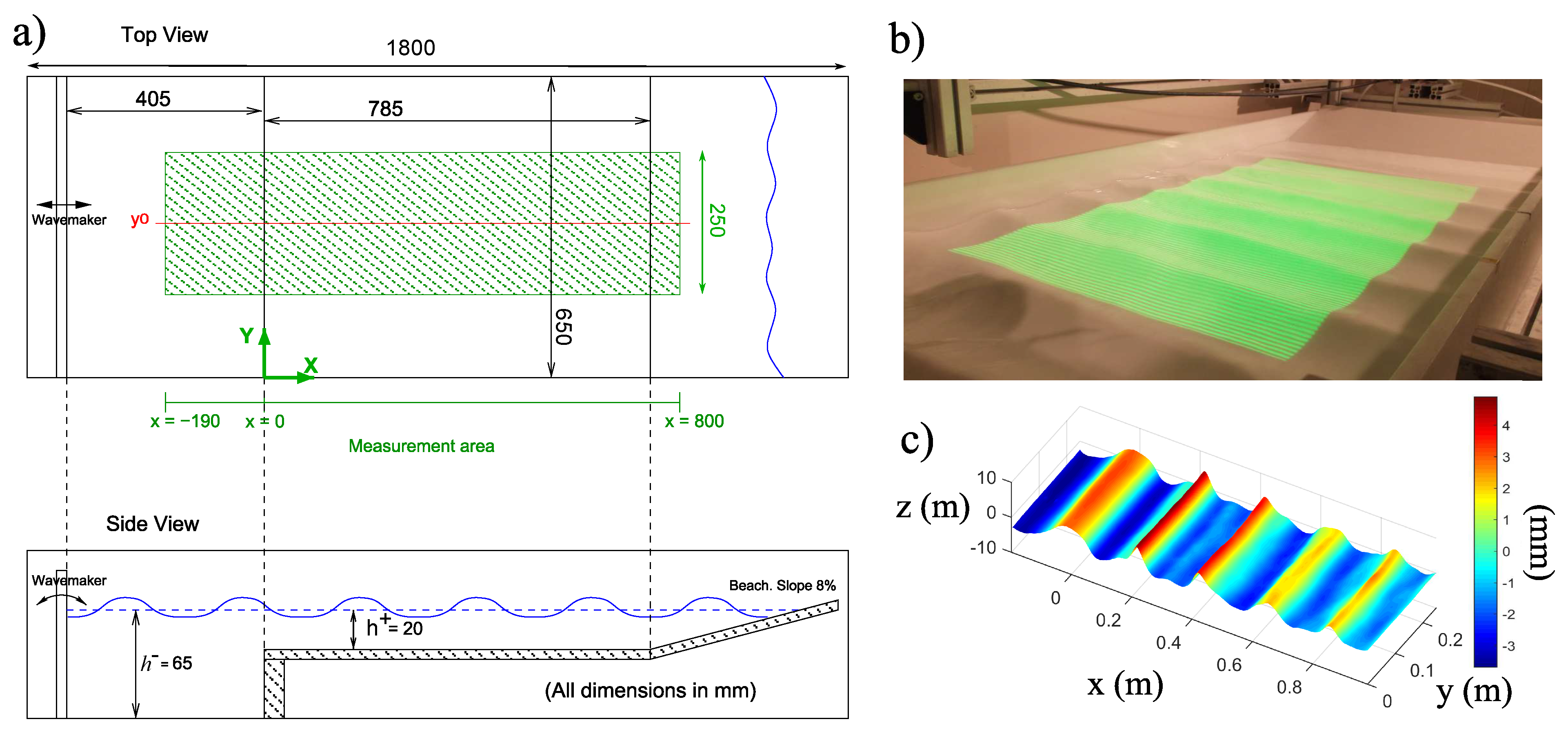
In this section, we present experimental space-time-resolved measurements of the propagation of nonlinear waves passing over a submerged step. The main objective of this section is provide quantitative measurements in such a way that the complex coefficients obtained in the multimodal model, especially for the second order, could be compared and validated with experiments. To do so, we take advantage of the Fourier transfer profilometry technique (FTP) to measure in space and time the surface deformation. In Figure 10a, we see a top view and a side view of the experimental setup. Experiments were carried out in a rectangular tank of 180 × 60 × 15 cm. A flap-type wavemaker is located 40 cm before the step from which waves propagate through a deep water region of 65 mm deep before passing over a rectangular step that separate the deep region from the shallow water region of 20 mm deep. The wave propagates 80 cm in the shallow region before attaining a 8% slope that avoid spurious reflections. As we see in Figure 10b, a sinosuidal pattern is projected onto a diffusive surface of water colored with titanuim dioxide (TiO₂), which does not change the water’s physical properties (Przadka et al. [31]). The post-treatment of the patter deformed by the wave motion allows measuring the surface height (see Figure 10c) in any point of the image. The measured field has a spatial resolution of 1700 × 400 pixels covering a surface of 1 m long and 25 cm large. The amplitude of the wavemaker was calibrated in such a way that the wave amplitude measured at the step was constant at $a\approx 3$ mm. The wave frequency with a monochromatic forcing varied in the range $\omega \in [10,20]$ ${\mathrm{s}}^{-1}$. Additionally, spurious capillary waves coming from the lateral boundaries and affecting the wave front were canceled by the use of a wire-mesh in the lateral walls, as conducted by Monsalve et al. [32,33]. As we shall observe in the following experimental results and considering the small scale of the experiments, the influence of the surface tension is non-negligible at the second order, where the wave number $k>100$ ${\mathrm{m}}^{-1}$. Despite this, the main results show that the multimodal model of gravity waves, presented in the theoretical section, fitted the experimental results well in terms of transmitted and reflected waves at the first and second order. Afterwards, along the spatial propagation, the second-order free and bound waves enhance the difference due to the surface tension as an extra restoring force in the dispersion relation.

Figure 10. Experimental set-up. (a) Sketch of the top and side views of the experimental tank. The measurement area is highlighted in green. (b) Experimental tank with the sinusoidal pattern of the FTP technique projected onto the diffusive surface. (c) Typical experimentally measured field of a nonlinear-wave.

4.2. Space-Time Spectra

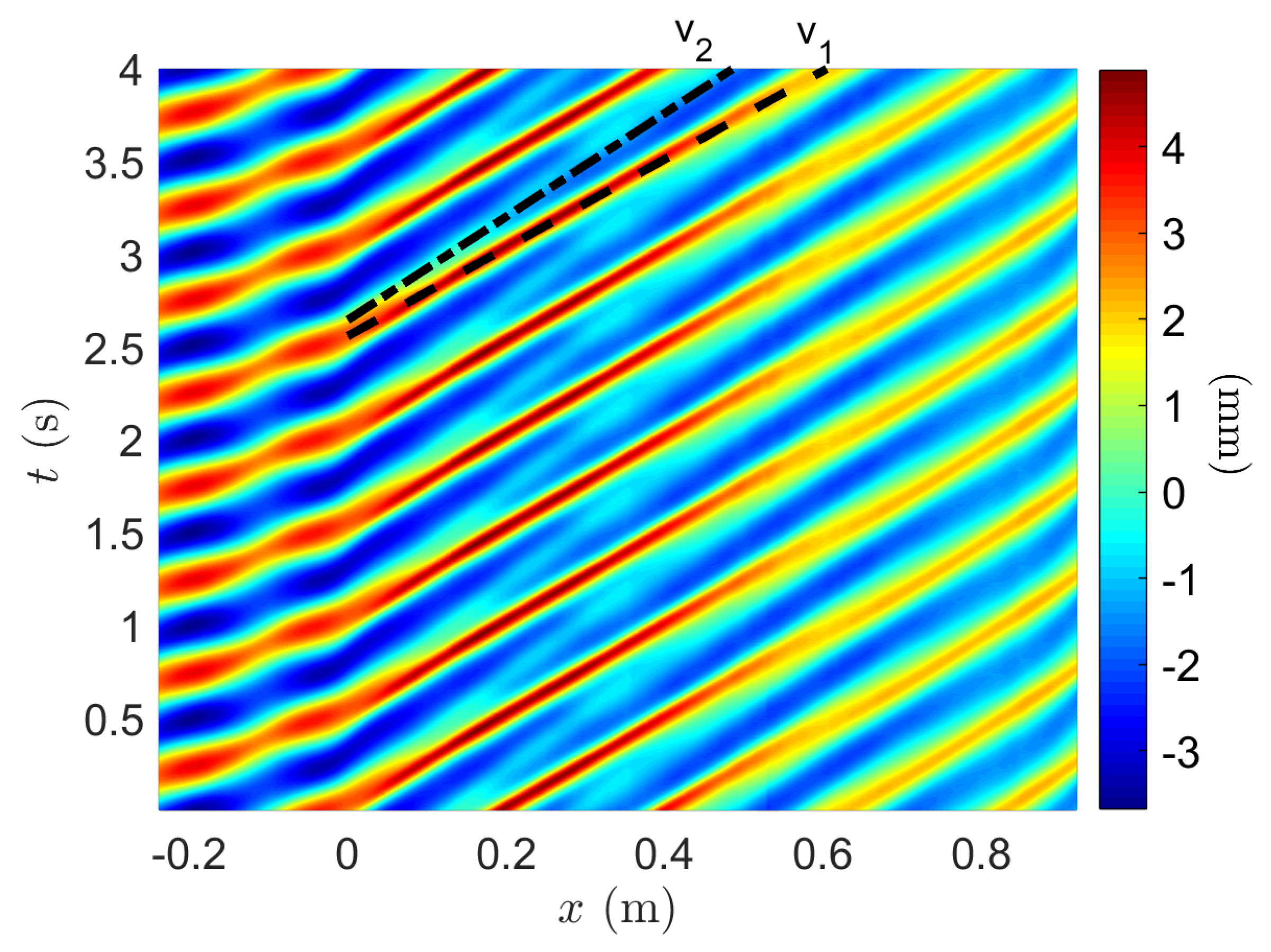
The measured field $\tilde{\eta }(x,y,t)$, considering that is invariant in the transverse direction y, is averaged in order to obtain a one-dimension measurement $\eta (x,t)$, which is presented as a space-time graph in Figure 11. Here, the origin of the abscissa is located at the step position. In $x<0$, the deep water region shows high modulation of the amplitude, indicating a high reflection from the step. On the other hand, in $x>0$, a narrower wave crest and a lager wave trough indicate nonlinear wave propagation. More interestingly, two different wave celerities, indicated as $V_1$ and $V_2$ in Figure 11, are clearly observed in the shallow water region. As we shall see further on, $V_2$ corresponds to the propagation of free waves at the second order.

Figure 11. Space-time representation of the wave propagation at $\omega =4\pi$ ${\mathrm{s}}^{-1}$ after transverse average in the y direction. Dashed and dashed-dotted lines shows two different celerities in the shallow water region.

From the space-time matrix $\eta (x,t)$, considering it in a harmonic regime, we can compute different temporal modes as

$${\eta }_n\left(x\right)=\frac{1}{T}{\int }_0^T\eta (x,t)e^{-in\omega t}dt,$$

(65)

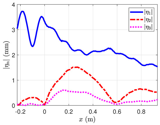
where T is the duration of the signal and is equal to an integer multiple of the wave period. The amplitude of the harmonics ${\eta }_1\left(x\right)$, ${\eta }_2\left(x\right)$ and ${\eta }_3\left(x\right)$, for the experiment carried out at $\omega =4\pi$ ${\mathrm{s}}^{-1}$, is presented in Figure 12. As we observe, $|{\eta }_1|$ has a large modulation due to the step reflection in the region $x<0$. In the region $x>0$, we observe large attenuation due to experimental conditions, such as bottom friction or surface impurities. The second harmonic $|{\eta }_2|$ has a clear beating in the shallow region, suggesting the spatial interference of waves at different velocities. Eventually, the third-order harmonic $|{\eta }_3|$ has a non-negligible amplitude that can be interesting to take into account. However, considering that the multimodal model only solves the first and second order, we focus on these two problems, leaving the third order to a future study.

Figure 12. Amplitude of the temporal harmonics $|{\eta }_n\left(x\right)$ with $n=1,2,3$ measured with Fourier transform profilometry at a frequency $\omega =4\pi$ ${\mathrm{s}}^{-1}$.

Once the harmonics are calculated, we compute a spatial Fourier transform as

$${\widehat{\eta }}_n\left(k\right)=\frac{1}{L}{\int }_0^L{\eta }_n\left(x\right)e^{-ikx}dx,$$

(66)

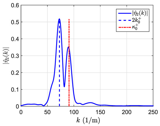
from which we can analyze the spatial spectral information at a given harmonic frequency $n\omega$. As an example, regardless of the spatial spectrum of the first harmonic that does not give any additional information, we show in Figure 13 the spatial spectrum of the second harmonic ${\eta }_2\left(k\right)$ measured at $\omega =4\pi$ ${\mathrm{s}}^{-1}$. Interestingly, we clearly distinguish two maxima corresponding to the free and the bound wave that propagates at this frequency. As a reference, two vertical lines have been added. First, on the left side, the wavenumber $2k_0^{+}$ corresponds to the bound wave, which is twice the wavenumber satisfying the dispersion relation of Equation (18), and second, on the right side, the wavenumber ${\kappa }_0^{+}$ corresponds to the free wave, which satisfies the dispersion relation of the second order of Equation (49). The experimental separation of free and bound waves is limited by the spectral resolution (total length of the spatial domain). Regarding the amplitude of both maxima, the dispersion of the waves represented by the relative depth of the experiment $k_0^{+}{h}^{+}$ determines the contribution of the free wave with respect to the bound wave. In the multimodal model, free waves are designed to ensure the matching of $\varphi$ and ${\partial }_x\varphi$ once the bound wave field is calculated. We observe that the higher the relative depth $k_0^{+}{h}^{+}$ is, the smoother the transition between both sides of the bound wave field ${\varphi }_2^b$ is (particular solutions of the second order) and the smaller the contribution of the free waves field ${\varphi }_2^f$ required to satisfy the matching conditions is. This trend shall be confirmed experimentally further on.

Figure 13. Amplitude of the second harmonic ${\eta }_2\left(k\right)$ as a function of wave number. Non-dimensional wavenumber of the linear mode is $k_0^{+}{h}^{+}$ = 0.73. Vertical lines indicate the wavenumber expected from the dispersion relation of water waves in Equation (49).

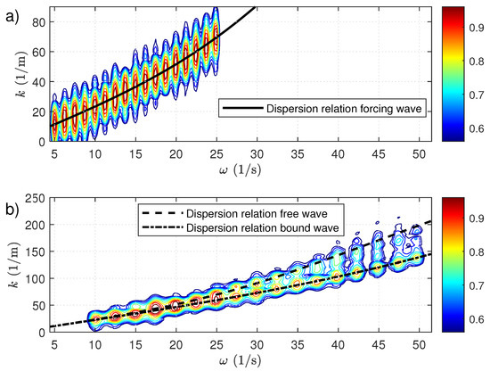
In order to give a general overview of the wave propagation, we show in Figure 14a,b the experimental dispersion relation at the first and second order, respectively. Here, we present the power spectrum $PS(\omega ,k)$ (in colored contours) normalized by its maximum value corresponding to the forcing wave—$PS(\omega ,k)/max\left[PS\right(\omega ,k\left)\right]$—which means that all maxima are equal to 1 in Figure 14a. In this graph, we have gathered an experimental series keeping only one experiment per frequency (when the number of experiments was more than one). Every spectrum in the plane $(\omega ,k)$ was normalized by its maximum value, which corresponds to the fundamental mode. More interestingly, at the second order, the dispersion relation of the bound and free waves follows different curves. Whereas bound waves have the same phase velocity as the fundamental mode $v_{\varphi }^b=2\omega /\left(2k_0\right)$, free waves propagate at a slower phase velocity $v_{\varphi }^f=2\omega /{\kappa }_0$. Additionally, from Figure 14b, we can observe the decay of the amplitude of the free wave as a function of the wave frequency. This decay shall be analyzed in comparison with the theoretical multimodal model.

Figure 14. Experimental dispersion relation in the plane $(\omega ,k)$. (a) Dispersion relation of the linear mode $\eta \left(\omega \right)$. (b) Dispersion relation of the second-order $\eta \left(2\omega \right)$.

4.3. Amplitude and Phase of Free and Bound Waves

We start by reconstructing the surface displacement of free and bound waves from the solution of the second-order potential ${\varphi }_2^f$ and ${\varphi }_2^b$. These complex valued coefficients shall be compared further on with experiments. Therefore, from the dynamic boundary condition of Equation (32), we can compute the free wave as

$${\eta }_2^f=-\frac{1}{g}\frac{\partial {\varphi }_2^f}{\partial t}$$

(67)

and the bound wave as

$${\eta }_2^b=-\frac{1}{g}\left[\frac{\partial {\varphi }_2^b}{\partial t}+\frac{1}{2}\left({\left(\frac{\partial {\varphi }_1}{\partial x}\right)}^2+{\left(\frac{\partial {\varphi }_1}{\partial z}\right)}^2\right)-\frac{1}{g}\frac{\partial {\varphi }_1}{\partial t}\frac{{\partial }^2{\varphi }_1}{\partial t\partial z}\right]$$

(68)

where ${\varphi }_2^b$ and ${\varphi }_2^f$ are the propagating terms of the total second-order solution (see Equation (35)). The free surface wave displacement is easily obtained from Equation (67); thus, we only give an explicit solution of ${\eta }_2^b$. Considering an incident wave $I_{0,0}^{(1,1)}(x,t)$ (as in Equation (36)), the velocity potential of the incident bound wave is

$${\varphi }_2^b=\frac{3}{8}\frac{\omega a^{2}cosh2k_0(z+h)}{{sinh}^4\left(k_{0}h\right)}sin2(k_{0}x-\omega t),$$

(69)

which can be replaced, together with the incident term of ${\varphi }_1=I_0^{\left(1\right)}{F}_0^{\left(1\right)}$, in Equation (68) to obtain the surface displacement of the incident bound wave

$${\eta }_2^b=\frac{1}{4}{a}^2{k}_0\left(2+cosh2k_{0}h\right)\frac{cosh{k}_{0}h}{{sinh}^3{k}_{0}h}cos2(k_{0}x-\omega t)-\frac{1}{2}\frac{a^2{k}_0}{sinh2k_{0}h}$$

(70)

where the last term, which is constant, corresponds to the shift in the mean water level due to the wave non-linearity (Stokes [34]).

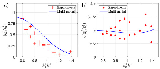
Next, we pass to the experimental validation of the theoretical waves ${\eta }_2^f$ and ${\eta }_2^b$. From the space-time Fourier transform, we can extract at the frequency of the second order ($2\omega$), the complex values of the free and bound waves corresponding to the local maxima shown in Figure 13. The ratio between the amplitudes of free and bound waves ($|{\eta }_2^f|/|{\eta }_2^b|$) is plotted in Figure 15a as a function of the non-dimensional wavenumber $k_0^{+}{h}^{+}$. The theoretical curve was calculated with the same experimental parameters: $h^{-}=0.065$ m, $h^{+}=0.02$ m, $a=0.003$ m and $\omega \in [10,20]$ ${\mathrm{s}}^{-1}$. We observe the decay of the theoretical curve that is well verified by the experimental points that are, however, mostly below the theoretical curve. This overestimation of the theoretical ratio with respect to the experiments may be explained by the actual attenuation due to the experimental conditions. The fact that the theory only solves the second order may also overestimate the contribution of this order to the total solution. To complement, the phase difference ($\theta ({\eta }_2^f/{\eta }_2^b)$) measured at the step position between the free and bound waves is plotted in Figure 15b. This phase difference, according to the multimodal model, should be close to $\pi$, i.e., waves have opposite phases evolving slightly with the wavenumber. However, experimentally, the fact that the relative amplitude of the free wave decays as a function of the wavenumber means the signal-to-noise ratio is not sufficiently high enough to detect the free wave phase; thus, the experimental points are only accurately measured in the range $k_0^{+}{h}^{+}<0.8$.

Figure 15. Experimental measurement and theoretical model of the second-order free and bound waves. (a) Amplitude ratio between free and bound waves $|{\eta }_2^f|/|{\eta }_2^b|$. (b) Phase different between free and bound waves measured at the step position $\theta \left({\eta }_2^f\right|/\left|{\eta }_2^b\right)$.

4.4. Beating Length and the Influence of the Surface Tension

The scale of the experimental set-up, in particular the shallow water depth $h^{+}=2$ cm, makes the second-order wavenumber be in the order of $k\approx 100$ ${\mathrm{m}}^{-1}$. At this scale, the influence of the surface tension in the dynamics of wave propagation starts to be non-negligible, as recently reported by Alippi et al. [35]. This is especially the case at the second order, where the high wavenumbers enhance the effect of the surface tension on the wave propagation. Actually, the wavenumber at the second-order free waves follows the dispersion relation of gravity-capillary waves

$${\omega }^2=\left(g{k}_0^{\pm }+\frac{\sigma }{\rho }{\left(k_0^{\pm }\right)}^3\right)tanh\left(k_0^{\pm }{h}^{\pm }\right),$$

(71)

where $\sigma$ is the surface tension and $\rho$ the density. As we observe in Figure 16, one of the clearest dimensions to be measured is the beating length of the second harmonic. This distance produced by the spatial interference between the free and bound waves is equal to the inverse of the wavenumber difference and reads

$$L_2=\frac{2\pi }{{\kappa }_0^{+}-2k_0^{+}}.$$

(72)

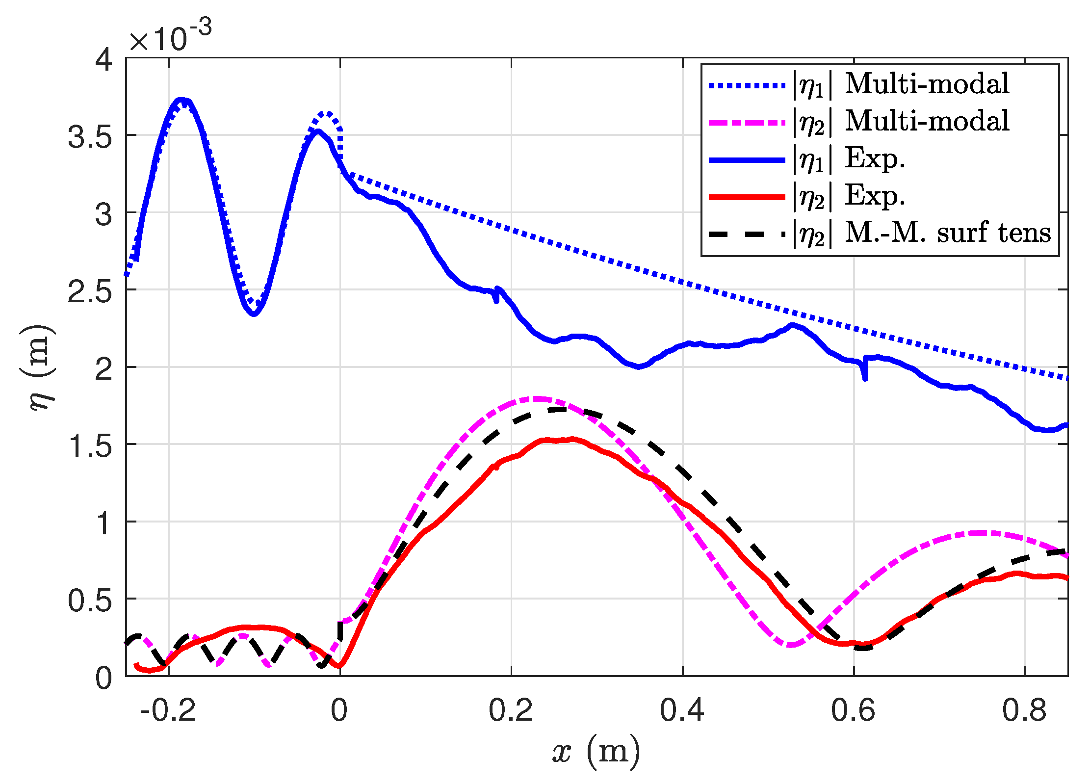
Figure 16. Comparison of the experimentally measured amplitude of the first (blue solid line) and second (red solid line) harmonics ($|{\eta }_1|$, $|{\eta }_2|$) with the propagating wave amplitudes computed in the multimodal model. At the second order, the theoretical beating is computed with (black dashed line) and without (magenta dash-dotted line) surface tension. Wave frequency $\omega =4\pi$ ${\mathrm{s}}^{-1}$.

In Figure 16, the experimental measured ${\eta }_2$ has a beating longer than the theoretical one. This mismatch is then corrected when the wavenumber of the propagating free and bound waves takes into account the surface tension, as in Equation (71). This addition of the surface tension has been included arbitrarily in the propagating wave after the multimodal calculation, which has been computed considering only a pure gravity regime.

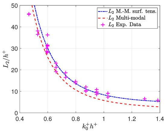
Eventually, in Figure 17, we gather the measurement of the beating length of the second-order $L_2$ for all the experiments. We plot the beating length from Equation (72) as a reference when $k_0^{+}$ and ${\kappa }_0^{+}$ are calculated from the dispersion relation of gravity waves in Equation (49) and when they are calculated from the dispersion relation of gravity capillary waves in Equation (71). As we see, the beating length follows different curves depending on the wavenumber. Whereas for small waveumbers the beating length seems to be dominated by the gravity regime, for large wavenumbers, the influence of the surface tension in the beating length is clear.

Figure 17. Beating length of the second harmonic ${\eta }_2$ as a function of the non-dimensional wavenumber $k_0^{+}{h}^{+}$. Two theoretical curves of $L_2$ are calculated from Equation (72): First, the blue dash-dotted line shows $L_2$ calculated with wavenumbers from Equation (71), and second, the red dashed line shows $L_2$ with wavenumbers from Equation (18).

5. Conclusions

In this article, we have revisited the multimodal model of the propagation of nonlinear waves over a submerged rectangular step proposed by Massel [6]. In this work, we focused on the problem of convergence that the model shows at the second order, where the bound evanescent waves, when calculated in the source term (right hand) of the kinematic and dynamic surface boundary conditions, produce a growth of the source term at a power $n^4$ that is higher than the decay exponent of the reflection and transmission coefficients of the first order, which are supposed to compensate for the divergence in the source term. This problem of convergence, although directly detectable when the model is correctly implemented, was not reported by Massel [6], apparently because the calculation was performed with only 20 modes. Nowadays, the computational power means the numerical computation can use a large number of modes at a low cost, which needs a robust implementation to ensures a convergent model independently of the number of modes. Therefore, by analyzing in detail the terms with the fastest growth in the source term that dominate the divergence of the second-order solution, we found that a truncation of the source term at a number of modes smaller than the first order produces convergence of the second-order problem, resulting in a smooth field in both potential ${\varphi }_2$ and horizontal velocity ${\partial }_x{\varphi }_2$. We found that the threshold of the number of modes in the source term $\alpha N^{\pm }$, with $\alpha \le 0.5$, ensures the convergence of the second-order solution. We have verified that this truncation works independently of the input parameters of the problem (geometry and wave characteristics) and has an error in the multimodal matching that decreases as a function of $N^{\pm }$. This convergence analysis can be useful to researchers interested in solving rectangular submerged obstacles in nonlinear wave problems.

The second part of the article shows the space-time-resolved measurement of the nonlinear wave propagation. This kind of measurement allows computing the complex coefficient (amplitude and phase) of the propagating waves at the first and second order. In particular, we were interested in the propagation of free and bound waves at the second order, where we have experimentally verified that the relative contribution of free waves decreases as a function of the non-dimensional wavenumber $k_0^{+}{h}^{+}$ (the system becomes more linear), and the phase between free and bound waves is the opposite at the step. Additionally, due to the scale of the experimental set-up, surface tension effects are non-negligible at the second order, where the wavenumber is in the order of $k\approx 100$ ${\mathrm{m}}^{-1}$. A systematic measurement of the beating length of the second harmonic reveals that at high wavenumbers ($k_0^{+}{h}^{+}>0.7$), the surface tension should be considered. An interesting continuation of this work may consider the development of the multimodal model with surface tension, which would make the solution more suitable to small-scale phenomena.

Appendix A.1. Solution of the System

The system of Equations (27) and (29) can be solved for $R_n^{\left(1\right)}$

$$\sum _n{R}_n^{\left(1\right)}\left({\partial }_x{A}_n^{\left(1\right)}{N}_n^{\left(1\right)}{\delta }_{n,\gamma }-\sum _m\frac{A_n^{\left(1\right)}{\partial }_x{B}_m^{\left(1\right)}{L}_{n,m}^{\left(1\right)}{L}_{\gamma ,m}^{\left(1\right)}}{M_m^{\left(1\right)}{B}_m^{\left(1\right)}}\right)=-{\partial }_x{I}_0^{\left(1\right)}{N}_0^{\left(1\right)}{\delta }_{0,\gamma }+\sum _m\frac{I_0^{\left(1\right)}{\partial }_x{B}_m^{\left(1\right)}{L}_{0,m}^{\left(1\right)}{L}_{\gamma ,m}^{\left(1\right)}}{M_m^{\left(1\right)}{B}_m^{\left(1\right)}}$$

(A1)

where ${\delta }_{k,\gamma }$ is the Kronecker delta, and the following notations were used to express the integrals:

$$L_{n,m}^{\left(1\right)}={\int }_{-h^{+}}^0{F}_n^{\left(1\right)}{G}_m^{\left(1\right)}$$

(A2)

$$M_m^{\left(1\right)}={\int }_{-h^{+}}^0{\left(G_m^{\left(1\right)}\right)}^2$$

(A3)

$$N_n^{\left(1\right)}={\int }_{-h^{-}}^0{\left(F_n^{\left(1\right)}\right)}^2$$

(A4)

The transmission coefficients $T_m^{\left(1\right)}$ can be easily obtained from Equation (27).

Appendix B.1. Constants

The bound wave constant $C_{n,n^{\prime }}^{(1,1)}$ obtained from the source term by replacing Equation (21) in the right-hand side of Equation (31) and performing lengthy algebraic manipulations

$$C_{n,n^{\prime }}^{(1,1)}=\frac{i{g}^2{a}^2}{2\omega }\frac{\left[\begin{array}{c}{\left(k_n^{-}\right)}^2+4k_n^{-}{k}_{n^{\prime }}^{-}+{\left(k_{n^{\prime }}^{-}\right)}^2-{\left(k_n^{-}\right)}^2{tanh}^2{k}_n^{-}{h}^{-}\hfill \\ \hfill -{\left(k_{n^{\prime }}^{-}\right)}^2{tanh}^2{k}_{n^{\prime }}^{-}{h}^{-}-4k_n^{-}{k}_{n^{\prime }}^{-}tanh{k}_n^{-}{h}^{-}tanh{k}_{n^{\prime }}^{-}{h}^{-}\end{array}\right]}{4{\omega }^2-g(k_n^{-}+k_{n^{\prime }}^{-})tanh(k_n^{-}+k_{n^{\prime }}^{-})h^{-}}.$$

(A5)

The constant $C_{0,n}^{(1,1)}$ of the second-order evanescent terms resulting from the multiplication of the Stokes incident harmonic with the evanescent reflected bound waves takes the following form

$$C_{0,n}^{(1,1)}=\frac{i{g}^2{a}^2}{2\omega }\frac{\left[\begin{array}{c}{\left(k_n^{-}\right)}^2-4k_0^{-}{k}_n^{-}+{\left(k_n^{-}\right)}^2-{\left(k_0^{-}\right)}^2{tanh}^2{k}_0^{-}{h}^{-}\hfill \\ \hfill -{\left(k_n^{-}\right)}^2{tanh}^2{k}_n^{-}{h}^{-}-4k_0^{-}{k}_n^{-}tanh{k}_0^{-}{h}^{-}tanh{k}_n^{-}{h}^{-}\end{array}\right]}{4{\omega }^2-g(k_0^{-}-k_n^{-})tanh(k_0^{-}-k_n^{-})h^{-}}.$$

(A6)

Appendix B.2. Solution of the System

The system of Equations (58) and (60) can be solved for $R_p^{\left(2\right)}$:

$$\begin{array}{c}{\displaystyle \sum _p}{R}_p^{\left(2\right)}\left({\partial }_x{A}_p^{\left(2\right)}{N}_p^{\left(2\right)}{\delta }_{p,\gamma }-{\displaystyle \sum _q}\frac{A_p^{\left(2\right)}{\partial }_x{B}_q^{\left(2\right)}{L}_{p,q}^{\left(2\right)}{L}_{\gamma ,q}^{\left(2\right)}}{M_q^{\left(2\right)}{B}_q^{\left(2\right)}}\right)+c.c.={\displaystyle \sum _m}{\displaystyle \sum _{m^{\prime }}}{T}_m^{\left(1\right)}{T}_{m^{\prime }}^{\left(1\right)}{\partial }_x{B}_{m,m^{\prime }}^{(1,1)}{\int }_{-h^{+}}^0{G}_{m,m^{\prime }}^{(1,1)}{F}_{\gamma }^{\left(2\right)}\hfill \\ \hfill -{\partial }_x{I}_{0,0}^{(1,1)}{\int }_{-h^{-}}^0{F}_{0,0}^{(1,1)}{F}_{\gamma }^{\left(2\right)}-{\displaystyle \sum _n}{\displaystyle \sum _{n^{\prime }}}{R}_n^{\left(1\right)}{R}_{n^{\prime }}^{\left(1\right)}{\partial }_x{A}_{n,n^{\prime }}^{(1,1)}{\int }_{-h^{-}}^0{F}_{n,n^{\prime }}^{(1,1)}{F}_{\gamma }^{\left(2\right)}-{\displaystyle \sum _n}{R}_n^{\left(1\right)}{\partial }_x{D}_{0,n}^{(1,1)}{\int }_{-h^{-}}^0{H}_{0,n}^{(1,1)}{F}_{\gamma }^{\left(2\right)}\\ +{\displaystyle \sum _q}\frac{{\partial }_x{B}_q^{\left(2\right)}{L}_{\gamma ,q}^{\left(2\right)}}{M_q^{\left(2\right)}{B}_q^{\left(2\right)}}\left(I_{0,0}^{(1,1)}{\int }_{-h^{+}}^0{F}_{0,0}^{(1,1)}{G}_q^{\left(2\right)}+{\displaystyle \sum _n}{\displaystyle \sum _{n^{\prime }}}{R}_n^{\left(1\right)}{R}_{n^{\prime }}^{\left(1\right)}{A}_{n,n^{\prime }}^{(1,1)}{\int }_{-h^{+}}^0{F}_{n,n^{\prime }}^{(1,1)}{G}_q^{\left(2\right)}+{\displaystyle \sum _n}{R}_n^{\left(1\right)}{D}_{0,n}^{(1,1)}{\int }_{-h^{+}}^0{H}_{0,n}^{(1,1)}{G}_q^{\left(2\right)}\right.\hfill \\ \hfill \left.-{\displaystyle \sum _m}{\displaystyle \sum _{m^{\prime }}}{T}_m^{\left(1\right)}{T}_{m^{\prime }}^{\left(1\right)}{B}_{m,m^{\prime }}^{(1,1)}{\int }_{-h^{+}}^0{G}_{m,m^{\prime }}^{(1,1)}{G}_q^{\left(2\right)}\right)+c.c.\end{array}$$

(A7)

Here, we have expressed some known integrals with the following notation

$$L_{p,q}^{\left(2\right)}={\int }_{-h^{+}}^0{F}_p^{\left(2\right)}{G}_q^{\left(2\right)},$$

(A8)

$$M_q^{\left(2\right)}={\int }_{-h^{+}}^0{\left(G_q^{\left(2\right)}\right)}^2,$$

(A9)

$$N_p^{\left(2\right)}={\int }_{-h^{-}}^0{\left(F_p^{\left(2\right)}\right)}^2.$$

(A10)

The transmission coefficients $T_q^{\left(2\right)}$ can be easily obtained from Equation (58).

References

- Li, Y.; Draycott, S.; Zheng, Y.; Lin, Z.; Adcock, T.A.; Van Den Bremer, T.S. Why rogue waves occur atop abrupt depth transitions. J. Fluid Mech. 2021, 919, R5. [Google Scholar] [CrossRef]
- Mei, C.C.; Black, J.L. Scattering of surface waves by rectagular obstacles in waters of finite depth. J. Fluid Mech. 1969, 38, 499–511. [Google Scholar] [CrossRef]
- Miles, J.W. Surface-wave scattering matrix for a shelf. J. Fluid Mech. 1967, 28, 755–767. [Google Scholar] [CrossRef]
- Newman, J. Propagation of water waves over an infinite step. J. Fluid Mech. 1965, 23, 399–415. [Google Scholar] [CrossRef]
- Grue, J. Nonlinear water waves at a submerged obstacle or bottom topography. J. Fluid Mech. 1992, 244, 455–476. [Google Scholar] [CrossRef] [Green Version]
- Massel, S.R. Harmonic generation by waves propagating over submerged step. Coast. Eng. 1983, 7, 357–380. [Google Scholar] [CrossRef]
- Belibassakis, K.A.; Athanassoulis, G.A. Extension of second-order Stokes theory to variable bathymetry. J. Fluids Mech. 2002, 464, 35–80. [Google Scholar] [CrossRef] [Green Version]
- Belibassakis, K.A.; Athanassoulis, G.A. A coupled-mode system with application to nonlinear water waves propagating in finite water depth and in variable bathymetry regions. Coast. Eng. 2011, 58, 337–350. [Google Scholar] [CrossRef]
- Athanassoulis, G.A.; Belibassakis, K.A. A consistent coupled-mode theory for the propagation of small amplitude water waves over variable bathymetry regions. J. Fluids Mech. 1999, 389, 275–301. [Google Scholar] [CrossRef] [Green Version]
- Rhee, J.P. On the transmission of water waves over a shelf. Appl. Ocean Res. 1997, 19, 161–169. [Google Scholar] [CrossRef]
- Porter, R.; Porter, D. Approximations to the scattering of water waves by steep topography. J. Fluids Mech. 2006, 562, 279–302. [Google Scholar] [CrossRef]
- Li, Y.; Zheng, Y.; Lin, Z.; Adcock, T.A.; van den Bremer, T.S. Surface wavepackets subject to an abrupt depth change. Part 1. Second-order theory. J. Fluid Mech. 2021, 915, A71. [Google Scholar] [CrossRef]
- Ducrozet, G.; Slunyaev, A.; Stepanyants, Y. Transformation of envelope solitons on a bottom step. Phys. Fluids 2021, 33, 066606. [Google Scholar] [CrossRef]
- Bryant, P.J. Periodic waves in shallow water. J. Fluid Mech. 1972, 59, 625–644. [Google Scholar] [CrossRef]
- Huang, C.J.; Dong, C.M. Wave deformation and vortex generation in water waves propagating over a submerged dike. Coast. Eng. 1999, 37, 123–148. [Google Scholar] [CrossRef]
- Chapalain, G.; Cointe, R.; Temperville, A. Observed and modeled resonantly interacting progressive water-waves. Coast. Eng. 1992, 16, 267–300. [Google Scholar] [CrossRef]
- Beji, S.; Battjes, J.A. Experimental investigation of wave propagation over a bar. Coast. Eng. 1992, 19, 151–162. [Google Scholar] [CrossRef]
- Li, F.; Ting, C. Separation of free and bound harmonics in waves. Coast. Eng. 2012, 67, 29–40. [Google Scholar] [CrossRef]
- Benoit, M.; Raoult, C.; Yates, M. Fully nonlinear and dispersive modeling of surf zone waves: Non-breaking tests. Coast. Eng. Proc. 2014, 1, 15. [Google Scholar] [CrossRef]
- Ohyama, T.; Nadaoka, K. Transformation of a nonlinear wave train passing over a submerged shelf without breaking. Coast. Eng. 1993, 24, 1–22. [Google Scholar] [CrossRef]
- Brossard, J.; Chagdali, M. Experimental investigation of the harmonic generation by waves over a submerged plate. Coast. Eng. 2001, 42, 277–290. [Google Scholar] [CrossRef]
- Brossard, J.; Perret, G.; Blonce, L.; Diedhiou, A. Higher harmonics induced induced by a submerged horizontal plate and a submerged rectangular step in a wave flume. Coast. Eng. 2009, 56, 11–22. [Google Scholar] [CrossRef]
- Ting, C.L.; Chao, W.T.; Young, C.C. Experimental investigation of nonliear regular waves transformation over submerged step: Harmonic generation and wave height modulation. Coast. Eng. 2016, 117, 19–31. [Google Scholar] [CrossRef]
- Ohyama, T.; Kioka, W.; Tada, A. Applicability of numerical models to nonlinear dispersive waves. Coast. Eng. 1995, 24, 297–313. [Google Scholar] [CrossRef]
- Takeda, M.; Ina, H.; Kobayashi, S. Fourier-transform method of fringe-pattern analysis for computer-based topography and interferometry. JosA 1982, 72, 156–160. [Google Scholar] [CrossRef]
- Takeda, M.; Mutoh, K. Fourier transform profilometry for the automatic measurement of 3-D object shapes. Appl. Opt. 1983, 22, 3977–3982. [Google Scholar] [CrossRef] [PubMed]
- Cobelli, P.; Maurel, A.; Pagneux, V.; Petitjeans, P. Global measurement on water waves by Fourier transform profilometry. Exp. Fluids 2009, 46, 1037–1047. [Google Scholar] [CrossRef]
- Hsu, J.R.C.; Tsuchiya, Y.; Silvester, R. Third order approximation to short crested waves. J. Fluids Mech. 1979, 90, 179–196. [Google Scholar] [CrossRef]
- Mei, C.C.; Stiassnie, M.; Yue, D.K.P. Theory and Applications of Ocean Surface Waves. Part 1: Linear Aspects; World Scientific: Singapore, 2005; Volume 23. [Google Scholar]
- Sommerfeld, A. Partial Differential Equations in Physics; Academic Press: Cambridge, MA, USA, 1949; Volume 1. [Google Scholar]
- Przadka, A.; Cabane, B.; Pagneux, V.; Maurel, A.; Petitjeans, P. Fourier transform profilometry for water waves: How to achieve clean water attenuation with diffusive reflection at the water surface? Exp. Fluids 2012, 52, 519–527. [Google Scholar] [CrossRef]
- Monsalve, E.; Maurel, A.; Petitjeans, P.; Pagneux, V. Perfect absorption of water waves by linear or nonlinear critical coupling. Appl. Phys. Lett. 2019, 114, 013901. [Google Scholar] [CrossRef] [Green Version]
- Monsalve, E.; Maurel, A.; Pagneux, V.; Petitjeans, P. Space-time-resolved measurements of the effect of pinned contact line on the dispersion relation of water waves. Phys. Rev. Fluids 2022, 7, 014802. [Google Scholar] [CrossRef]
- Stokes, G.G. On the theory of the oscillatory waves. Trans. Camb. Phil. Soc. 1847, 8, 441–455. [Google Scholar]
- Alippi, A.; Bettucci, A.; Germano, M. Model and experiments for resonant generation of second harmonic capillary–gravity waves. Phys. D Nonlinear Phenom. 2019, 396, 12–17. [Google Scholar] [CrossRef]
Publisher’s Note: MDPI stays neutral with regard to jurisdictional claims in published maps and institutional affiliations. |
© 2022 by the authors. Licensee MDPI, Basel, Switzerland. This article is an open access article distributed under the terms and conditions of the Creative Commons Attribution (CC BY) license (https://creativecommons.org/licenses/by/4.0/).