Traveling-Standing Water Waves

Abstract

We propose a new two-parameter family of hybrid traveling-standing (TS) water waves in infinite depth that evolve to a spatial translation of their initial condition at a later time. We use the square root of the energy as an amplitude parameter and introduce a traveling parameter that naturally interpolates between pure traveling waves moving in either direction and pure standing waves in one of four natural phase configurations. The problem is formulated as a two-point boundary value problem and a quasi-periodic torus representation is presented that exhibits TS-waves as nonlinear superpositions of counter-propagating traveling waves. We use an overdetermined shooting method to compute nearly 50,000 TS-wave solutions and explore their properties. Examples of waves that periodically form sharp crests with high curvature or dimpled crests with negative curvature are presented. We find that pure traveling waves maximize the magnitude of the horizontal momentum among TS-waves of a given energy. Numerical evidence suggests that the two-parameter family of TS-waves contains many gaps and disconnections where solutions with the given parameters do not exist. Some of these gaps are shown to persist to zero-amplitude in a fourth-order perturbation expansion of the solutions in powers of the amplitude parameter. Analytic formulas for the coefficients of this perturbation expansion are identified using Chebyshev interpolation of solutions computed in quadruple-precision.

1. Introduction

Traveling and standing water waves have been studied extensively since the pioneering work of Stokes [1] and Rayleigh [2] (see e.g., [3,4,5,6,7,8,9,10,11,12,13,14,15,16] and the references therein). The goal of the present work is to study hybrid traveling-standing water waves that evolve to an exact replica of their initial condition, but shifted in space. Pure traveling and standing waves will be included in the family as special cases. Unifying these classes of solutions of the water wave equations leads to new dynamic behavior and reveals a bifurcation structure similar to that observed in integrable model equations such as the Benjamin–Ono equation [17,18,19]. Water wave solutions also exhibit major differences, which we will highlight, from those of integrable model equations.

One of the main challenges that arises immediately when considering traveling-standing waves is determining how best to parameterize the solutions in the family. For the amplitude parameter, we use the square root of a dimensionless energy, $\epsilon =\sqrt{E}$, which is a natural choice on physical grounds. However, defining a “traveling” parameter is difficult. We propose a parameter $\beta$ that measures the relative amplitude of the right-moving and left-moving components of the fundamental spatial mode of the TS-wave. Solutions related by spatial translation, time reversal, or temporal translation turn out to correspond to shifting $\beta$ by $\pi$ or reflecting it about 0 or $\pi /2$, which makes it easier to work with than momentum to identify different waves in the family with the same energy. Intuitively, we may conjecture that pure traveling waves should maximize or minimize the momentum among traveling-standing waves of a given energy. We confirm this numerically for low to moderate amplitude, though there are small-divisor issues that call into question the tacit assumption in this conjecture that traveling-standing waves occur in smooth families. We present numerical evidence that resonances lead to disconnections running through the family of solutions. It is possible that with infinite precision, solutions would only exist for values of $\epsilon$ and $\beta$ in Cantor-like sets. Rigorous proofs of existence suggest that this is the case for pure standing waves [20,21,22] and various classes of quasi-periodic water waves [23,24,25,26,27].

Rayleigh’s third order perturbation expansion for “stationary” standing waves [2] was carried out in sufficient generality to also recover Stokes’ progressive waves, but he did not consider hybrid waves possessing features of both stationary and progressive waves. Pierce and Knobloch [28] note that weakly nonlinear standing waves can be thought of as nonlinear superpositions of equal amplitude left- and right-traveling (LTW and RTW) wave trains. They work within a Davey–Stewartson model for finite-depth water waves with surface tension and propose a wider family of quasi-periodic solutions containing arbitrary superpositions of LTW and RTW waves. They then study the stability of these waves with respect to long wavelength longitudinal and transverse perturbations. Bridges and Laine-Pearson [29] also regard standing waves as synchronized counter-propagating periodic traveling waves and show that within a weakly nonlinear Schrödinger equation model, standing waves are modulationally unstable only if the component traveling waves are modulationally unstable. They embed standing waves in a four-parameter family of counter-propagating waves, construct a variational principle for this larger family in a multi-symplectic Hamiltonian framework (which puts space and time on an equal footing), and then take the limit to the original two-parameter family of standing waves to determine their stability properties. In Section 3.3, we will show how to represent traveling-standing water waves on a torus as a special case of the counter-propagating wave representation of Bridges and Laine-Pearson. This aligns our results with other recent studies of temporally quasi-periodic water waves [23,24,25,26,27].

In the present work, for simplicity, we consider only irrotational gravity waves without surface tension in infinite depth. The numerical method is a generalization (from pure standing waves to TS-waves) of the overdetermined shooting algorithm of Wilkening [12] and Wilkening and Yu [13]. The shooting method is formulated as an overdetermined nonlinear least squares problem using the leading Fourier modes of the initial condition as the unknowns. This improves efficiency and robustness since we only solve for Fourier modes that are well-resolved on the grid. Higher-frequency modes are set to zero in the initial condition but still penalized if they grow in amplitude when evolved through a cycle of the dynamics.

A finite-depth variant of the methods of this paper is given in [30] to study relative-periodic elastic collisions of co-propagating soliton-like solutions of the fully nonlinear water wave equations on a spatially periodic domain. Unlike the present work, amplitude and traveling parameters $\epsilon$ and $\beta$ are not used in [30] to explore families of solutions via numerical continuation. Instead, a few large-amplitude solutions are found using initial guesses obtained from linear superpositions of traveling Stokes waves that are well-separated in space to limit their initial nonlinear interaction. These water wave solutions are compared quantitatively and qualitatively with cnoidal solutions of the Korteweg–deVries (KdV) equation in [30]. A major contribution of the present work is to systematically study the entire two-parameter family of traveling-standing waves in infinite depth rather than focusing attention on just a few solutions.

The idea for the present study of traveling-standing water waves originated in a study of the harmonic stability of pure standing waves in infinite depth [31]. In a Floquet analysis, the monodromy operator of a pure standing wave was always found to possess two independent Jordan chains [32] associated with the eigenvalue $\lambda =1$. In general, degenerate eigenvalues in which the algebraic multiplicity exceeds the geometric multiplicity give rise to secular growth when the monodromy operator is applied repeatedly. For standing water waves, one of the Jordan chains at $\lambda =1$ corresponds to perturbing the amplitude parameter. A slight change in period causes the perturbed standing wave to drift away from the unperturbed standing wave with a deviation that grows linearly in time. However, the second Jordan chain observed in [31] was a surprise. It points to a perturbation that drifts away from the base standing wave through small translations in space that grow linearly with successive cycles. The only reference to such waves we have seen in the literature is a parenthetical comment by Iooss, Plotnikov, and Toland [21]: “It is possible to imagine more general solutions, for example, ‘travelling-standing-wave’ solutions, of the free boundary problem.” As mentioned already, Pierce and Knobloch [28] and Bridges and Laine-Pearson [29] encounter the same types of waves by independently varying the amplitude of counter-propagating wave trains within weakly nonlinear theory. However, our formulation as a two-point boundary value problem, in which the solution returns to a spatial translation of the initial condition, appears to be new.

This paper is organized as follows. In Section 2, we recall the graph-based formulation of the water wave equations and describe our time-stepping algorithm as well as the boundary integral method we use to compute the Dirichlet–Neumann operator. In Section 3.1, we define traveling-standing water waves, introduce the amplitude and traveling parameters $\epsilon$ and $\beta$, and demonstrate how the TS-solutions fit together. In Section 3.2 and Appendix A, we present the overdetermined shooting method we use to compute fully nonlinear TS-waves and show how to compute the Jacobian matrix efficiently in parallel. In Section 3.3, we present a quasi-periodic torus representation for TS-waves and make connections with the work of Bridges and Laine-Pearson [29], Berti et al. [25,26], and Feola and Giuliani [27]. In Section 4, we present numerical results showing how the period, spatial phase shift, horizontal momentum, and curvature at the origin of the initial wave profile depend on the amplitude and traveling parameters. In Section 4.1 and Section 4.2, we compute additional solutions to explore the gaps and disconnections that arise in the two-parameter family where solutions could not be found numerically. We contrast these results with the global paths of time-periodic solutions that connect pairs of traveling waves of the Benjamin–Ono equation and also study various types of “extreme” TS-waves. In Section 5, we use Chebyshev interpolation in quadruple-precision to identify analytic formulas for a fourth order asymptotic expansion of both the initial conditions and the quasi-periodic torus representation of the solution in powers of the amplitude parameter. We find that the most prominent disconnections in the two-parameter family of TS-waves persist to zero-amplitude, where they manifest as coefficients in the asymptotic expansion that diverge as $\beta$ approaches $\{\pm \frac{\pi }{12},\pm \frac{5\pi }{12},\pm \frac{7\pi }{12},\pm \frac{11\pi }{12}\}$. Alternative amplitude and traveling parameters are discussed in Section 5.3. Concluding remarks are given in Section 6.

2. Equations of Motion and Time-Stepping

To compute traveling-standing water waves, we employ a shooting method, which requires an accurate timestepper. For simplicity, we consider only the case of pure gravity waves (with zero surface tension) evolving over a two-dimensional ideal fluid of infinite depth. The waves are assumed to be spatially periodic in x, and after non-dimensionalization [31], the period may be assumed to be $2\pi$. The free surface is denoted by $\eta (x,t)$ and the velocity potential in the fluid is denoted by $\Phi (x,y,t)$. The surface velocity potential, $\phi$, is the restriction of $\Phi$ to the free surface,

$$\phi (x,t)=\Phi (x,\eta (x,t),t).$$

(1)

The equations of motion governing $\eta$ and $\phi$ may be written [33,34,35]:

$$\begin{array}{cc}\hfill {\eta }_t& =\mathcal{G}\left(\eta \right)\phi ,\hfill \\ \hfill {\phi }_t& =P\left[\frac{1}{2}\left(\frac{{\left(G\left(\eta \right)\phi +{\eta }_x{\phi }_x\right)}^2}{1+{\eta }_x^2}-{\phi }_x^2\right)-g\eta \right],\hfill \end{array}$$

(2)

where subscripts denote partial derivatives; g is the acceleration of gravity, which may be set to 1 after non-dimensionalization [31]; $\mathcal{G}\left(\eta \right)$ is the Dirichlet–Neumann operator [13,34,35]; and P is the $L^2$ projection to zero mean that annihilates constant functions,

$$P=id-P_0,P_{0}f=\frac{1}{2\pi }{\int }_0^{2\pi }f\left(x\right)dx.$$

(3)

Including this projection in the ${\phi }_t$ equation yields a convenient convention for selecting the arbitrary additive constant in the potential. In infinite depth, the projection has no effect for the continuous problem if the mean surface height is zero. However we still include it in the numerical algorithm since a drift in the mean value of $\phi$ due to floating-point errors affects the objective function in the shooting method for computing traveling-standing waves. The Dirichlet–Neumann operator is defined via:

$$\mathcal{G}\left(\eta \right)\phi \left(x\right)=\sqrt{1+{\eta }^{\prime }{\left(x\right)}^2}\frac{\partial \Phi }{\partial n}(x,\eta \left(x\right))={\Phi }_y-{\eta }_x{\Phi }_x,$$

(4)

where $\Phi (x,y)$ is the solution of the Laplace equation with periodic boundary conditions in x, Dirichlet boundary conditions ($\Phi =\phi$) on the upper boundary, and Neumann boundary conditions at $y=-\infty$, i.e., ${lim}_{y\to -\infty }{\Phi }_y(x,y)=0$. We have suppressed t in the notation since time is frozen in the Laplace equation. We note that ${\phi }_x$ in (2) and ${\Phi }_x$ in (4) are different quantities. The former is the x-derivative of $\phi (x,t)$, which is how it is computed, while the latter is the restriction to the free surface of ${\Phi }_x(x,y,t)$, which is defined throughout the fluid.

To compute the Dirichlet–Neumann operator in (4), we use the boundary integral method described in [13], which builds on previous boundary integral methods for irrotational flow problems [7,36,37,38,39,40,41]. Given the wave profile $\eta \left(x\right)$ and Dirichlet data $\phi \left(x\right)$, the method amounts to solving the integral equation:

$$\frac{1}{2}\mu \left(\alpha \right)+\frac{1}{2\pi }{\int }_0^{2\pi }K(\alpha ,\beta )\mu \left(\beta \right)d\beta =\phi \left(\alpha \right)$$

(5)

for the dipole density $\mu \left(x\right)$, and then computing:

$$\mathcal{G}\left(\eta \right)\phi \left(\alpha \right)=\frac{1}{2}H\left[{\mu }^{\prime }\right]\left(\alpha \right)+\frac{1}{2\pi }{\int }_0^{2\pi }G(\alpha ,\beta ){\mu }^{\prime }\left(\beta \right)d\beta .$$

(6)

Here a prime denotes differentiation and H is the Hilbert transform, which may be written as a principal value integral, $Hf\left(\alpha \right)=\frac{1}{\pi }PV{\int }_0^{2\pi }\frac{f\left(\beta \right)}{2}cot\left(\frac{\alpha -\beta }{2}\right)d\beta$. The Hilbert transform is diagonal in Fourier space with symbol:

$${\widehat{H}}_k=-isgn\left(k\right)=\left\{\begin{array}{cc}-i,\hfill & k>0,\hfill \\ 0,\hfill & k=0,\hfill \\ i,\hfill & k<0.\hfill \end{array}\right.$$

(7)

This makes it easy to compute using the FFT. The formulas for the kernels K and G are:

$$\begin{array}{c}\hfill K(\alpha ,\beta )=Im\left\{\frac{{\zeta }^{\prime }\left(\beta \right)}{2}cot\left(\frac{\zeta \left(\alpha \right)-\zeta \left(\beta \right)}{2}\right)-\frac{1}{2}cot\left(\frac{\alpha -\beta }{2}\right)\right\},\\ \hfill G(\alpha ,\beta )=Re\left\{\frac{{\zeta }^{\prime }\left(\alpha \right)}{2}cot\left(\frac{\zeta \left(\alpha \right)-\zeta \left(\beta \right)}{2}\right)-\frac{1}{2}cot\left(\frac{\alpha -\beta }{2}\right)\right\},\end{array}$$

(8)

Here $\zeta \left(\alpha \right)=\alpha +i\eta \left(\alpha \right)$ parameterizes the free surface in the complex plane, which we have identified with ${\mathbb{R}}^2$. Equations (5) and (6) are derived in [13] by assuming the complex velocity potential $W\left(z\right)$ at a point $z=x+iy$ in the fluid has the form:

$$W\left(z\right)=\frac{1}{2\pi i}{\int }_0^{2\pi }\frac{{\zeta }^{\prime }\left(\alpha \right)}{2}cot\left(\frac{z-\zeta \left(\alpha \right)}{2}\right)d\alpha .$$

(9)

One then takes limits of $\Phi \left(z\right)=\mathrm{Re}\left\{W\right(z\left)\right\}$ and ${\Phi }_x\left(z\right)-i{\Phi }_y\left(z\right)=W^{\prime }\left(z\right)$ as z approaches the point $(\alpha +i\eta (\alpha \left)\right)$ on the free surface using the Plemelj formula [42]. We have regularized the principal value integrals from the Plemelj formula by including the term $\frac{1}{2}cot\left(\frac{\alpha -\beta }{2}\right)$ in $K(\alpha ,\beta )$ and $G(\alpha ,\beta )$, which makes them continuous, periodic, and real analytic (assuming $\eta \left(x\right)$ has these properties) if we define:

$$K(\alpha ,\alpha )=Im\left\{-\frac{{\zeta }^{″}\left(\alpha \right)}{2{\zeta }^{\prime }\left(\alpha \right)}\right\},G(\alpha ,\alpha )=Re\left\{-\frac{{\zeta }^{″}\left(\alpha \right)}{2{\zeta }^{\prime }\left(\alpha \right)}\right\}$$

(10)

Dropping the regularizing term from the formula for K has no effect since its imaginary part is zero; including this term in the definition of G is accounted for by the Hilbert transform in (6). We solve the integral Equation (5) using a Nyström collocation method based on the trapezoidal rule on a uniformly spaced M-point grid,

$$\frac{1}{2}{\mu }_i+\frac{1}{M}\sum _{j=0}^{M-1}K({\alpha }_i,{\alpha }_j){\mu }_j={\phi }_i,(0\le i\le M-1)$$

(11)

where ${\alpha }_j=2\pi j/M$ for $0\le j\le M-1$. We also evaluate $\mathcal{G}\left(\eta \right)\phi$ in (6) via the trapezoidal rule. This method of evaluating $G\left(\eta \right)\phi$ is spectrally accurate due to the real analyticity and periodicity of $K(\alpha ,\beta )$ and $G(\alpha ,\beta )$. See [13] for details.

For time-stepping (2), we use an 8th order Runge–Kutta scheme [43] in double-precision (DOPRI8), and a 15th order spectral deferred correction method [44,45,46] in quadruple-precision (SDC15). We also make use of the 36th order filter popularized by Hou, Lowengrub, and Shelley [38] and Hou and Li [47]. This filter consists of multiplying the kth Fourier mode by:

$$exp\left[-36{\left(\left|k\right|/k_{\max }\right)}^{36}\right],k_{\max }=M/2,$$

(12)

which strikes a balance between suppressing aliasing errors and resolving high-frequency modes.

As mentioned already, we assume the waves are spatially periodic and choose units of length and time so that the wavelength is $2\pi$ and the acceleration of gravity is $g=1$. We also choose units of mass so the fluid density is $\rho =1$, which will be relevant when computing the energy and momentum of these solutions below. An explicit non-dimensionalization procedure is given in [31].

3. Traveling-Standing Water Waves

In this section we define traveling-standing waves, focusing on solutions of the water wave equations with certain symmetry properties. We then define amplitude and traveling parameters and describe a trust-region shooting method for computing traveling-standing waves with given values of these parameters via numerical continuation. This method will be used in Section 4 and Section 5 below to study a two-parameter family of solutions bifurcating from the flat rest state.

3.1. Formulation as a Two-Point Boundary Value Problem

We define a traveling-standing water wave as a solution of (2) for which there is a $T>0$ and $\theta \in \mathbb{R}$ such that the solution exists for $t\in [0,T]$ and:

$$\begin{array}{c}\hfill \eta (x,T)=\eta (x-\theta ,0),\\ \hfill \phi (x,T)=\phi (x-\theta ,0),\end{array}$$

(13)

i.e., the solution returns to a spatial translation of the initial condition at a later time, $t=T$. Since the water wave equations are translation invariant and time-reversible, (13) implies that the solution exists for all positive and negative times and satisfies:

$$\begin{array}{cc}\hfill \eta (x,t+T)& =\eta (x-\theta ,t),\hfill \\ \hfill \phi (x,t+T)& =\phi (x-\theta ,t),\hfill \end{array}(x,t\in \mathbb{R}).$$

(14)

If $\theta =0$, the wave is time-periodic and T is its period. Actually, the condition (13) is unchanged if we add an integer multiple of the wavelength (=2$\pi$) to $\theta$, and we will see below that the most natural choice of $\theta$ for pure standing waves as a special case of traveling-standing waves is $\theta =2\pi$.

Pure standing waves are symmetric [7,13,14] time-periodic solutions with phases often chosen so that $\eta (x,0)$ is an even, $2\pi$-periodic function and $\phi (x,0)\equiv 0$. For pure standing waves, at time $T/2$, the wave comes to rest again, shifted in space by $\pi$ (so $\eta (x,T/2)=\eta (x-\pi ,0)$ and $\phi (x,T/2)\equiv 0$). It returns to its starting configuration at $t=T$. If one shifts time by a quarter period, one may instead assume that $\eta (x,0)$ and $\phi (x,0)$ are even, $2\pi$-periodic functions satisfying:

$$\eta (x+\pi ,0)=\eta (x,0),\phi (x+\pi ,0)=-\phi (x,0).$$

(15)

In this case, the solution will return to its initial state at time T if it comes to rest at time $T/4$,

$$\phi (x,T/4)=0,0\le x\le 2\pi .$$

(16)

This symmetry was exploited in [7,13] to save a factor of 4 in computational time over a “brute-force” time-periodic calculation, similar to that of [18], over $0\le t\le T$.

For traveling-standing waves, it is too restrictive to require that $\phi (·,t)\equiv 0$ at some time t. However, we have found alternative symmetry conditions that lead to computational savings similar to those of conditions (15) and (16) but include richer families of solutions. The first requirement is that the initial conditions satisfy:

$$\eta (x,0)\mathrm{is}\mathrm{even},\phi (x,0)\mathrm{is}\mathrm{odd}.$$

(17)

Pure standing waves have this form in the first convention described above, where $t=0$ corresponds to $\phi \equiv 0$. Within the second convention of (15) and (16), we can obtain the form (17) if we shift time by $T/4$ to get back the first convention, or, alternatively, if we shift the spatial phase of the initial conditions by $\pi /2$. Here we note that if $\eta (x,0)$ and $\phi (x,0)$ are even and satisfy (15), then $x\mapsto \eta (x-\pi /2,0)$ and $x\mapsto \phi (x-\pi /2,0)$ are even and odd functions, respectively. In general, when (17) is satisfied, the functions ${\eta }_1(x,t)=\eta (-x,-t)$, ${\phi }_1(x,t)=-\phi (-x,-t)$ are solutions of the Euler equations with the same initial conditions as $\eta$ and $\phi$; thus, ${\eta }_1=\eta$ and ${\phi }_1=\phi$. Now suppose there are numbers T and $\theta$ such that:

$$\eta (x+\theta /4,T/4)\mathrm{is}\mathrm{even},\phi (x+\theta /4,T/4)\mathrm{is}\mathrm{odd}.$$

(18)

Then,

$$\begin{array}{cc}\hfill \eta (x+\theta /4,T/4)& =\eta (-x+\theta /4,T/4)=\eta (x-\theta /4,-T/4),\hfill \\ \hfill \phi (x+\theta /4,T/4)& =-\phi (-x+\theta /4,T/4)=\phi (x-\theta /4,-T/4)\hfill \end{array}$$

(19)

and

$$\begin{array}{cc}\eta (x,t+T/2)\hfill & =\eta (x-\theta /2,t),\hfill \\ \phi (x,t+T/2)\hfill & =\phi (x-\theta /2,t),\hfill \end{array}$$

(20)

since both sides agree at time $t=-T/4$. Thus, the wave returns to a spatial translation of its initial condition at a later time, as required. Pure standing waves are a special case (with $\theta =2\pi$). Note that $\eta (x,t+T)=\eta (x,t)$ in that case, which is why we call T the period rather than $T/2$. The computational savings remains a factor of 4 over a naive time-periodic calculation since $\eta$ and $\phi$ only have to be evolved over a quarter period to confirm that (18) holds. Pure traveling waves satisfy (14) for any T and $\theta$ satisfying $\theta =cT$, where c is the wave speed. We define the period as the value of T where the bifurcation to this family of traveling-standing waves occurs.

To classify traveling-standing waves, we need two parameters, one governing the amplitude and one specifying the extent to which the wave is traveling. A natural choice for the former is the average energy per unit length,

$$E=\frac{\rho }{\lambda }{\int }_0^{\lambda }\frac{1}{2}\phi \mathcal{G}\phi +\frac{1}{2}g{\eta }^{2}dx,(\rho =1,g=1,\lambda =2\pi ).$$

(21)

We instead use

$$\epsilon =\sqrt{E}$$

(22)

as the amplitude parameter since E depends quadratically on $\eta$ and $\phi$ at small amplitude (where $\mathcal{G}\left(\eta \right)\approx \mathcal{G}\left(0\right)=H{\partial }_x$.) For the “traveling parameter,” we propose:

$$\beta = atan2\left(e^{i\theta /4}{\widehat{\eta }}_1(T/4),{\widehat{\eta }}_1\left(0\right)\right),$$

(23)

where ${\widehat{\eta }}_1\left(t\right)$ is the first spatial Fourier mode of $\eta (x,t)$ and $atan2(b,a)=arg(a+ib)$ is the angle from the positive x-axis to the point $(a,b)\in {\mathbb{R}}^2$. Since $\eta (x,0)$ is even and (18) holds, both arguments of the function $atan2(b,a)$ in (23) are real. We next motivate the definition (23) and show that shifting $\beta$ by $\pi$ or reflecting it about 0 or $\pi /2$ leads to an identical solution up to a spatial or temporal phase shift or reflection.

In the linearized regime where (2) is approximated by

$${\eta }_t=H{\phi }_x,{\phi }_t=-g\eta$$

(24)

and $\mathcal{G}$ in (21) is approximated by $H{\partial }_x$, the general solution of (2) with wave number $k=1$ that satisfies (17)–(20) and (21)–(23) has the form:

$$\begin{array}{c}\hfill \eta (x,t)=2\epsilon \left(sin\beta sintsinx+cos\beta costcosx\right),\\ \hfill \phi (x,t)=2\epsilon \left(sin\beta costsinx-cos\beta sintcosx\right),\end{array}$$

(25)

where $T=\theta =2\pi$ in (18) and (23). These functions may also be written:

$$\begin{array}{cc}\eta (x,t)\hfill & =\sqrt{2}\epsilon \left[cos\left(\beta -\frac{\pi }{4}\right)cos(x-t)-sin\left(\beta -\frac{\pi }{4}\right)cos(x+t)\right],\hfill \\ \hfill \phi (x,t)& =\sqrt{2}\epsilon \left[cos\left(\beta -\frac{\pi }{4}\right)sin(x-t)+sin\left(\beta -\frac{\pi }{4}\right)sin(x+t)\right],\hfill \end{array}$$

(26)

which expresses the solution as a superposition of counter-propagating traveling waves and serves as a starting point for defining the torus representation of Section 3.3 below. Note that $\beta$ governs the relative amplitude of the right- and left-moving component traveling waves. From (25), we see that the first Fourier mode of $\eta (x,t)$ evolves in time via:

$${\widehat{\eta }}_1\left(t\right)=\epsilon (cos\beta cost-isin\beta sint).$$

(27)

Thus, as illustrated in the left panel of Figure 1, the trajectories of ${\widehat{\eta }}_1\left(t\right)$ in this linearized setting are ellipses oriented along the real or imaginary axis. These ellipses cross the coordinate axes at $x=\pm cos\beta$, $y=\pm sin\beta$. Thus, $\beta$ may be regarded as a measure of the eccentricity $e={\left[1-min({tan}^2\beta ,{cot}^2\beta )\right]}^{1/2}$ of the orbit of ${\widehat{\eta }}_1\left(t\right)$, but with additional phase information specifying which of the two points where the ellipse crosses the x-axis corresponds to $t=0$ and whether the ellipse is traversed clockwise or counter-clockwise as t increases. Setting $T=\theta =2\pi$ in this linearized setting, we have:

$${\widehat{\eta }}_1\left(0\right)=\epsilon cos\beta ,e^{i\theta /4}{\widehat{\eta }}_1(T/4)=\epsilon sin\beta ,$$

(28)

which motivates the definition (23).

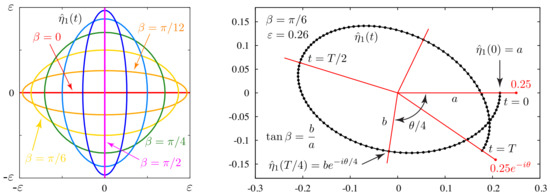
Figure 1. Trajectories of ${\widehat{\eta }}_1\left(t\right)$ in the linearized regime (left) and nonlinear regime (right). These trajectories are ellipses in the linearized regime and generate roulette-like shapes at larger amplitudes when the phase shift $\theta$ deviates from $2\pi$.

At larger amplitudes, the orbit of ${\widehat{\eta }}_1\left(t\right)$ will no longer be elliptical, but the maxima and minima of $|{\widehat{\eta }}_1\left(t\right)|$ still occur when t is an integer multiple of $T/4$. We are only able to prove that $|{\widehat{\eta }}_1\left(t\right)|$ has critical points at such t values. However, we observe numerically that these critical points correspond to extrema for all the solutions we have computed. Using (20) together with $\eta (x,-t)=\eta (-x,t)$, which follows from (17) as explained above, one finds that $q\left(t\right)=e^{i\theta t/T}{\widehat{\eta }}_1\left(t\right)$ satisfies:

$$q(t+T/2)=q\left(t\right),q(-t)=\overline{q\left(t\right)},q(T/4-t)=\overline{q(T/4+t)},(t\in \mathbb{R}).$$

(29)

It follows that $|{\widehat{\eta }}_1\left(t\right)|$ has even symmetry with respect to reflection about $t=nT/4$ for any integer n. Such reflection points are always critical points. Let $a=q\left(0\right)={\widehat{\eta }}_1\left(0\right)$ and $b=q(T/4)=e^{i\theta /4}{\widehat{\eta }}_1(T/4)$, which are both real. Periodicity of q implies that:

$${\widehat{\eta }}_1(nT/4)= \left\{\begin{array}{cc}a{e}^{-in\theta /4},\hfill & n\mathrm{even},\hfill \\ b{e}^{-in\theta /4},\hfill & n\mathrm{odd}.\hfill \end{array}\right.$$

(30)

At intermediate times, ${\widehat{\eta }}_1\left(t\right)$ sweeps out hypotrochoid-like curves resembling flower petals as it passes through the apsides (30) at times $t=nT/4$. This is illustrated in the right panel of Figure 1 for a traveling-standing wave with $\beta =\pi /6$, $\epsilon =0.26$, and $\theta =6.8825=2\pi +0.1908\pi$. The orbits of ${\widehat{\eta }}_1\left(t\right)$ for $t\in [nT,(n+1\left)T\right]$ will be identical to the $n=0$ case shown in the figure, but rotated clockwise by $n(\theta -2\pi )$ radians.

Several traveling-standing wave solutions with amplitude $\epsilon =0.25$ are shown in Figure 2. Our method of computing these waves will be explained in Section 3.2 below. The aim of Figure 2 is to provide a better understanding of the traveling parameter $\beta$ and the symmetries associated with changes in $\beta$. Solution A is a pure standing wave that begins at rest with $\eta (x,0)$ an even function of x with a peak at the origin. At $t=T/2$, the solution comes to rest again with the peak translated to $x=\pi$, consistent with (20). This standing wave corresponds to $\beta =0$. Solution D is a pure right-moving traveling wave. It corresponds to $\beta =\pi /4$. Solutions B and C are intermediate traveling-standing waves that have features of both A and D. Solutions B and C correspond to $\beta =\pi /12$ and $\beta =\pi /6$, respectively. Solutions A, B, and C are closely related to solutions G, F, and E through the transformation rules of Table 1. This will be discussed further below.

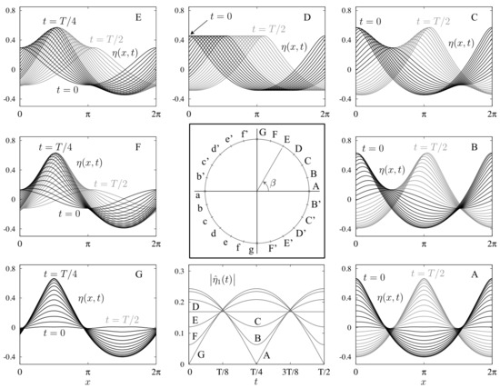
Figure 2. Dependence of traveling-standing waves on the traveling parameter $\beta$. Solutions (A–G) are shown in black from $t=0$ to $t=T/4$ and in grey from $13T/48$ to $T/2$. Each of the solution shown has energy $E=0.0625$. Pure standing waves (A, G, a, and g) correspond to ${\widehat{\eta }}_1\left(0\right)=0$ or ${\widehat{\eta }}_1(T/4)=0$, (so $\beta \in \{0,\pm \pi /2,\pi \}$). Pure traveling waves (D, D’, d, and d’) correspond to $|{\widehat{\eta }}_1(T/4)|= |{\widehat{\eta }}_1\left(0\right)|$, (so $\beta \in \{\pm \pi /4,\pm 3\pi /4\}$). In solution G, the grey curves are hidden behind the black curves.

Table 1. Transformation rules for shifting and reflecting $\beta$.

	Change in $\mathit{\beta }$, $\mathit{\theta }$	Effect
1.	${\beta }_{\mathrm{new}}=\beta +\pi$,  ${\theta }_{\mathrm{new}}=\theta$	Translation in space by $\pi$.
2.	${\beta }_{\mathrm{new}}=-\beta$,  ${\theta }_{\mathrm{new}}=4\pi -\theta$	Time reversal (or spatial reflection about $x=0$).
3.	${\displaystyle {\beta }_{\mathrm{new}}=\frac{\pi }{2}-\beta }$,  ${\theta }_{\mathrm{new}}=\theta$	Translation in space and time by $\theta /4$, $T/4$.

The bottom center panal of Figure 2 confirms that $|{\widehat{\eta }}_1\left(t\right)|$ passes through its maximum and minimum values when t is an integer multiple of $T/4$. Each curve $|{\widehat{\eta }}_1\left(t\right)|$ in this plot is shown from $0\le t\le T/2$ relative to its own period T, where T varies slightly for each solution in the plot (aside from $T_A=T_G$, $T_B=T_F$, and $T_C=T_E$). Note that $|{\widehat{\eta }}_1\left(t\right)|$ is constant in time at the traveling wave solution D and reaches zero only for the standing waves A and G. The same results would hold for the traveling waves D’, d, and d’ as well as the standing waves g and a, which are labeled on the “$\beta$ circle” in the center panel of Figure 2 but not plotted.

Once solutions are known in the range $0\le \beta \le \pi /4$, they are known for all $\beta$ up to changes in spatial and temporal phase or direction of travel. Table 1 gives the required transformation rules. A brief justification is as follows:

$$\begin{array}{cc}\hfill & 1.\left\{\begin{array}{c}\mathrm{Let}{\eta }_{\mathrm{new}}(x,t)=\eta (x+\pi ,t)\mathrm{and}{\phi }_{\mathrm{new}}(x,t)=\phi (x+\pi ,t).\hfill \\ \mathrm{Then}{\widehat{\eta }}_1\left(0\right)\mathrm{and}{\widehat{\eta }}_1(T/4)\mathrm{both}\mathrm{change}\mathrm{sign},\mathrm{so}|{\beta }_{\mathrm{new}}-\beta |=\pi .\hfill \end{array}\right.\hfill \\ \hfill & 2.\left\{\begin{array}{c}\mathrm{Let}{\eta }_{\mathrm{new}}(x,t)=\eta (x,-t),{\phi }_{\mathrm{new}}(x,t)=-\phi (x,-t),\mathrm{and}{\theta }_{\mathrm{new}}=4\pi -\theta .\hfill \\ \mathrm{Then}{\eta }_{\mathrm{new}}(x+{\theta }_{\mathrm{new}}/4,T/4)=\eta (x+\pi +\theta /4,T/4).\hfill \\ \mathrm{Result}:e^{i\theta /4}{\widehat{\eta }}_1(T/4)\mathrm{changes}\mathrm{sign},{\widehat{\eta }}_1\left(0\right)\mathrm{is}\mathrm{unchanged},\mathrm{and}{\beta }_{\mathrm{new}}=-\beta .\hfill \end{array}\right.\hfill \\ \hfill & 3.\left\{\begin{array}{c}\mathrm{Let}{\eta }_{\mathrm{new}}(x,t)=\eta (x+\theta /4,t+T/4)\mathrm{and}{\phi }_{\mathrm{new}}=\phi (x+\theta /4,t+T/4).\hfill \\ \mathrm{Then}{\eta }_{\mathrm{new}}(x,0)=\eta (x+\theta /4,T/4)\mathrm{and}{\eta }_{\mathrm{new}}(x+\theta /4,T/4)=\eta (x,0).\hfill \\ \mathrm{Result}:\mathrm{the}\mathrm{arguments}\mathrm{of}atan2(y,x)\mathrm{interchange},\mathrm{so}{\beta }_{\mathrm{new}}=\pi /2-\beta .\hfill \end{array}\right.\hfill \end{array}$$

For example, in the center panel of Figure 2, upper-case letters are related to lower-case letters via the first type of transformation in Table 1, and adding or removing primes corresponds to the second type of transformation. Solutions A, B, and C on the right in Figure 2 are related to those on the left (G, F, and E) by the third type of transformation, where $\beta$ is reflected across the ${45}^{\circ }$ line passing through points D and d on the circle in the center panel of Figure 2. As a result, the curves labeled $t=T/4$ in the left panels are spatial phase shifts of those labeled $t=T/2$ in the right panels. In particular, a pure standing wave satisfying the symmetry conditions (15) and (16) takes the form of solution A if time is shifted by $T/4$, or takes the form of solution G if space is shifted by $\pi /2$. One of these two phase shifts (or their negative counterparts) is required to satisfy condition (17), and varying $\beta$ from 0 to $\pi /2$ connects the phase shifted versions of the original standing wave together by traveling-standing waves of the same energy.

3.2. Trust-Region Shooting Method

To compute traveling-standing waves, we pose the problem as an overdetermined nonlinear system of equations. We solve this system using a variant of the Levenberg–Marquardt method in which the Jacobian updates are delayed over several accepted steps. See [13] for further details about this algorithm, including how to vary the trust-region radius when the Jacobian computation is lagged in this way.

From (17) and (18), we seek solutions in which $\eta (x,0)$ and $\eta (x+\theta /4,T/4)$ are even functions of x while $\phi (x,0)$ and $\phi (x+\theta /4,T/4)$ are odd. Let ${\widehat{\eta }}_j\left(t\right)$ and ${\widehat{\phi }}_j\left(t\right)$ denote the Fourier modes of the solution. As explained in more detail below, we choose an even integer $N\le 2M/3$, where M is the number of spatial gridpoints used in the timestepping algorithm, and consider initial conditions of the form:

$${\widehat{\eta }}_j=c_{2\left|j\right|-1},{\widehat{\phi }}_j=isgn\left(j\right)c_{2\left|j\right|},$$

(31)

where $j\in \{\pm 1,\pm 2,\cdots ,\pm \frac{N}{2}\}$. The numbers $c_1,\cdots ,c_N$ are assumed to be real and all other Fourier modes are set to zero. In the formula for ${\widehat{\phi }}_j$, $sgn\left(j\right)=-1$ if $j<0$ so that ${\widehat{\phi }}_{-j}=\overline{{\widehat{\phi }}_j}$. We also set:

$$T=c_{N+1},\theta =c_{N+2},$$

(32)

where T is the period and $\theta$ is the spatial phase shift in (18). We choose an objective function that is zero if and only if $\eta (x+\theta /4,T/4)$ and $\phi (x+\theta /4,T/4)$ are even and odd functions of x, respectively, and E in (21) and $\beta$ in (23) are equal to the given target values $E_0$, ${\beta }_0$. Specifically, we define:

$$f\left(c\right)=\frac{1}{2}r{\left(c\right)}^{T}r\left(c\right),$$

(33)

with

$$\begin{array}{cccc}\hfill r_1& =E-E_0,\hfill & \hfill r_{2j+1}& =Im\left\{e^{ij\theta /4}{\widehat{\eta }}_j(T/4)\right\},\hfill \\ \hfill r_2& =\beta -{\beta }_0,\hfill & \hfill r_{2j+2}& =Re\{e^{ij\theta /4}{\widehat{\phi }}_j(T/4)\},\hfill \end{array}(1\le j\le M/2),$$

(34)

where $\beta = atan2 \left(Re\{e^{i\theta /4}{\widehat{\eta }}_1(T/4)\},{\widehat{\eta }}_1\left(0\right)\right)$. Taking the real part of the first argument is necessary since $\eta (x+\theta /4,T/4)$ is not generally an even function until f has been driven to zero. Assuming ${\widehat{\eta }}_j(T/4)$ and ${\widehat{\phi }}_j(T/4)$ are zero for $\left|j\right|\ge M/2$, we then have:

$$\begin{array}{cc}\hfill f\left(c\right)& =\frac{1}{8\pi }{\int }_0^{2\pi }{\left(\frac{\eta (x+\theta /4,T/4)-\eta (-x+\theta /4,T/4)}{2}\right)}^{2}dx+\frac{1}{2}{(E-E_0)}^2\hfill \\ \hfill & +\frac{1}{8\pi }{\int }_0^{2\pi }{\left(\frac{\phi (x+\theta /4,T/4)+\phi (-x+\theta /4,T/4)}{2}\right)}^{2}dx+\frac{1}{2}{(\beta -{\beta }_0)}^2.\hfill \end{array}$$

(35)

We have assumed here that ${\widehat{\phi }}_0(T/4)=0$. This is true since ${\widehat{\phi }}_0\left(0\right)=0$ by construction and the projection P in (2) keeps ${\widehat{\phi }}_0\left(t\right)$ constant.

The number of spatial gridpoints, M, should be chosen large enough that for all times $t\in [0,T/4]$, the Fourier modes ${\widehat{\eta }}_j\left(t\right)$ and ${\widehat{\phi }}_j\left(t\right)$ decay to machine precision for $\left|j\right|\ge M/p$, where $p=2$ is required and $p=3$ is recommended to avoid aliasing errors when evaluating the nonlinearities of (2) and approximating the integrals (5) and (6) via the trapezoidal rule (11). By contrast, N only needs to be large enough that the Fourier modes ${\widehat{\eta }}_j$ and ${\widehat{\phi }}_j$ in (31) of the initial condition decay to machine precision by the time $\left|j\right|$ reaches $N/2$. For smaller-amplitude waves, we find that $N\approx 2M/3$ typically works well. The remaining Fourier modes of the initial condition are taken to be zero. This “zero padding” causes the number of equations, $M+2$, to be larger than the number of unknowns, $N+2$.

In some cases N can be substantially smaller than M, which makes the method more efficient as only lower-frequency Fourier modes of the initial condition have to be computed. This also improves the robustness of the shooting method since these lower-frequency modes are well-resolved on the M-point grid. Moreover, following the approach of Appendix A, all the columns of the Jacobian are obtained by computing well-resolved solutions of the linearized water wave equations corresponding to perturbations of the initial conditions in the direction of these lower-frequency modes. This allows the Jacobian to be computed accurately by discretizing the linearized water wave equations rather than having to linearize the discretized solution of the nonlinear problem. A common scenario where N can be much smaller than M is when $t=0$ corresponds to a relatively flat state while $t=T/4$ corresponds to a crested state with high curvature near the wave peak. In this scenario, there are often many more active Fourier modes (with mode amplitude larger than machine precision) in the final state than in the initial state. Thus, it is better to compute solutions E, F, and G than C, B, and A in Figure 2 as the former reach crested states at $T/4$ while the latter begin with crested states.

This idea of recasting shooting methods as overdetermined nonlinear systems was introduced in [13] to compute extreme standing waves. In that work, adaptive mesh refinement in both time and space was also used to better resolve the wave peak that emerges at $t=T/4$. For both pure standing waves and the generalization considered here to traveling-standing waves, because the solution returns to a spatial phase shift of the initial condition at $t=T/2$ (and again at $t=T$), if modes ${\widehat{\eta }}_j\left(t\right)$ and ${\widehat{\phi }}_j\left(t\right)$ with $\left|j\right|>N/2$ have become active at $t=T/4$, they decay back down to machine precision if time is further evolved from $t=T/4$ to $t=T/2$. At time $T/2$, each mode will differ from its initial state by only a phase factor, i.e., its amplitude will return to its initial value. This time-periodic transfer of energy between low- and high-frequency modes under the fully nonlinear water wave equations might be interesting to study through the lens of dynamic energy cascades [48,49].

3.3. A Quasi-Periodic Torus Representation of Traveling-Standing Water Waves

In Section 3.1, we formulated the traveling-standing water wave problem as a two-point boundary value problem with initial conditions of the form (17) that evolve from $t=0$ to $T/4$ to a state of the form (18). Amplitude and traveling parameters $\epsilon$ and $\beta$ are also specified to further constrain the solution through (22) and (23). All of these conditions involve properties of the solution at $t=0$ and $T/4$, with behavior at intermediate times determined only by the requirement that the equations of motion (2) hold. This is the most convenient formulation for computing such waves in a shooting framework.

Rigorous proofs of existence of time-periodic [20,21,22] and temporally quasi-periodic [23,24] standing water waves take a different approach, modeled on KAM theory, where periodicity or quasi-periodicity in time is built into the function space in which a Nash–Moser iteration is performed to enforce the equations of motion in the limit. In other words, in a shooting framework, successive approximations satisfy the evolution equations but not the temporal boundary conditions while in a KAM approach, each iteration satisfies the boundary conditions but not the evolution equations. In this section we consider torus representations of traveling-standing water waves that could potentially be used in a Nash–Moser iteration to prove their existence.

One idea is to define a function ${\tilde{Z}}_1({\xi }_1,{\xi }_2)$ that is periodic on the torus ${\mathbb{T}}^2={\mathbb{R}}^2/2\pi {\mathbb{Z}}^2$ such that:

$$Z(x,t)= \left(\begin{array}{c}\eta (x,t)\\ \phi (x,t)\end{array}\right) ={\tilde{Z}}_1\left(x-(\theta -2\pi )\frac{t}{T},2\pi \frac{t}{T}\right),$$

(36)

where $\theta$ is the spatial shift of (13), which we recall is taken to be $2\pi$ for pure standing waves. Periodicity of ${\tilde{Z}}_1({\xi }_1,{\xi }_2)$ on ${\mathbb{T}}^2$ ensures that $Z(x,T)=Z(x-\theta ,0)$, which is (13). A more general torus representation, namely:

$$Z(x,t)=\tilde{Z}\left(k_{1}x+{\omega }_{1}t,k_{2}x+{\omega }_{2}t\right),$$

(37)

was introduced by Bridges and Laine-Pearson [29] to study the stability of weakly nonlinear standing waves. This torus representation allows us to more clearly interpret traveling-standing water waves as nonlinear superpositions of counter-propagating periodic wave trains. The parameters $k_i$ and ${\omega }_i$ will be shown below to correspond to a rotation of the above torus function by ${45}^{\circ }$, i.e.,

$$\tilde{Z}({\theta }_1,{\theta }_2)={\tilde{Z}}_1\left(\frac{{\theta }_1-{\theta }_2}{2},\frac{{\theta }_1+{\theta }_2}{2}\right).$$

(38)

Pierce and Knobloch [28] studied weakly nonlinear interactions of such wave trains using a Davey–Stewartson model for finite-depth water waves with surface tension without employing torus representations of the solutions. Bridges and Laine-Pearson [29] expanded on these results using a completely different approach.

Solutions of the form (37) can describe a wide variety of wave phenomena. The spatially quasi-periodic traveling water waves considered by Bridges and Dias [50] within weakly nonlinear theory and by Wilkening and Zhao [51] in a fully nonlinear setting have the form (37) if one takes ${\omega }_1=-k_{1}c$ and ${\omega }_2=-k_{2}c$, where c is the wave speed. One recovers periodic traveling waves if $\tilde{Z}$ is independent of ${\theta }_1$ or ${\theta }_2$. Bridges and Laine-Pearson [29] note that pure standing waves have the form (37) if:

$${\omega }_1={\omega }_2=\omega ,k_1=-k_2=k,\tilde{Z}({\theta }_1,{\theta }_2)=\tilde{Z}({\theta }_2,{\theta }_1).$$

(39)

Indeed, after non-dimensionalization, if $\eta (x,0)$ and $\phi (x,0)$ are even, $2\pi$-periodic functions satisfying (15) and (16), we can define:

$$\tilde{Z}({\theta }_1,{\theta }_2)=Z\left(\frac{{\theta }_1-{\theta }_2}{2k},\frac{{\theta }_1+{\theta }_2}{2\omega }\right),Z(x,t)=\left(\begin{array}{c}\eta (x,t)\\ \phi (x,t)\end{array}\right),$$

(40)

where $k=1$ and $\omega =2\pi /T$. It then follows that $Z(x,t)=\tilde{Z}(\omega t+kx,\omega t-kx)$, as claimed. The function $\tilde{Z}({\theta }_1,{\theta }_2)$ in (40) is periodic on the torus ${\mathbb{T}}^2$ since $Z(x,t+T/2)=Z(x-\pi ,t)$. It is also symmetric with respect to interchanging ${\theta }_1$ and ${\theta }_2$ since $Z(x,t)$ is an even function of x for fixed t. Shifting time by $T/4$ does not change these symmetry properties, so solution A of Figure 2 also leads to a function $\tilde{Z}({\theta }_1,{\theta }_2)$ that is symmetric with respect to interchanging ${\theta }_1$ and ${\theta }_2$ when defined via (40).

General traveling-standing waves, including pure standing waves in the configuration of solution G in Figure 2, do not have torus functions satisfying (39) and (40). Instead, we claim that solutions of (2) satisfying (17) and (18) have the form:

$$Z(x,t)=\tilde{Z}({\omega }_{1}t+kx,{\omega }_{2}t-kx).$$

(41)

Solving ${\theta }_1={\omega }_{1}t+kx$ and ${\theta }_2={\omega }_{2}t-kx$ for x and t yields:

$$\tilde{Z}({\theta }_1,{\theta }_2)=Z\left(\frac{{\omega }_2{\theta }_1-{\omega }_1{\theta }_2}{({\omega }_1+{\omega }_2)k},\frac{{\theta }_1+{\theta }_2}{{\omega }_1+{\omega }_2}\right).$$

(42)

This function is periodic on the torus ${\mathbb{T}}^2$ if we set:

$$k=1,{\omega }_1=\frac{4\pi -\theta }{T},{\omega }_2=\frac{\theta }{T},$$

(43)

which follows from $Z(x+\theta /2,t+T/2)=Z(x,t)$ and $Z(x-2\pi ,t)=Z(x,t)$. Substitution of (43) into (42) gives the formulas for x and t reported in Figure 3. This confirms the ${45}^{\circ }$ rotation (38).

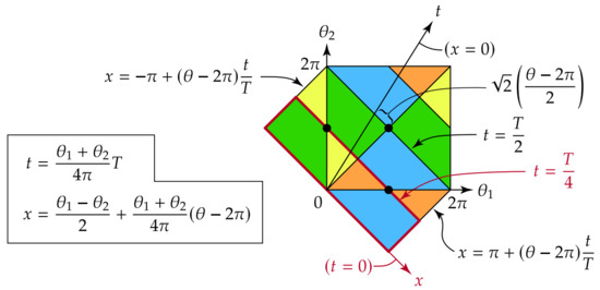
Figure 3. Correspondence between the physical variables $x,t$ and the torus variables ${\theta }_1,{\theta }_2$ in the representation (41). The rotated rectangle with a thick red border corresponds to $0\le t\le T/4$, which is the time range computed by our shooting algorithm. The values of $\tilde{Z}({\theta }_1,{\theta }_2)$ in this rectangle can be extended to fill the torus ${\mathbb{T}}^2$ using the rotational symmetries (46) about the three lattice points shown with black markers.

Next we define an operator R that acts on Z or $\tilde{Z}$ by reversing the sign of the velocity potential,

$$RZ(x,t)= \left(\begin{array}{c}\eta (x,t)\\ -\phi (x,t)\end{array}\right),R\tilde{Z}({\theta }_1,{\theta }_2)= \left(\begin{array}{c}\tilde{\eta }({\theta }_1,{\theta }_2)\\ -\tilde{\phi }({\theta }_1,{\theta }_2)\end{array}\right).$$

(44)

Using $Z(-x,-t)=RZ(x,t)$, which follows from (17) using the same argument we used to derive (19), we obtain:

$$\tilde{Z}(-{\theta }_1,-{\theta }_2)=R\tilde{Z}({\theta }_1,{\theta }_2).$$

(45)

Together with periodicity of $\tilde{Z}({\theta }_1,{\theta }_2)$ on ${\mathbb{T}}^2$, (45) implies that:

$$\tilde{Z}(n_1\pi +{\theta }_1,n_2\pi +{\theta }_2)=R\tilde{Z}(n_1\pi -{\theta }_1,n_2\pi -{\theta }_2),(n_1,n_2)\in {\mathbb{Z}}^2.$$

(46)

This rotational symmetry (with a sign change in the velocity potential) about lattice points in $\pi {\mathbb{Z}}^2$ can be used to construct $\tilde{Z}({\theta }_1,{\theta }_2)$ from $Z(x,t)$ with $0\le t\le T/4$, see Figure 3.

Next we note the effect of the transformation rules of Table 1 on $\tilde{Z}({\theta }_1,{\theta }_2)$. If ${\beta }_{\mathrm{new}}={\beta }_{\mathrm{old}}+\pi$, then $\theta$ remains unchanged and:

$${\tilde{Z}}_{\mathrm{new}}\left({\theta }_1,{\theta }_2\right) =Z_{\mathrm{new}}\left(x,t\right) =Z_{\mathrm{old}}\left(x+\pi ,t\right) ={\tilde{Z}}_{\mathrm{old}}\left({\theta }_1+\pi ,{\theta }_2-\pi \right),$$

(47)

where x and t depend on ${\theta }_1$ and ${\theta }_2$ through the formulas in Figure 3. Similarly, if ${\beta }_{\mathrm{new}}=-{\beta }_{\mathrm{old}}$, then ${\theta }_{\mathrm{new}}=4\pi -{\theta }_{\mathrm{old}}$ and:

$${\tilde{Z}}_{\mathrm{new}}({\theta }_1,{\theta }_2) =Z_{\mathrm{new}}\left(x,t\right) =Z_{\mathrm{old}}\left(-x,t\right) ={\tilde{Z}}_{\mathrm{new}}({\theta }_2,{\theta }_1).$$

(48)

In addition, if ${\beta }_{\mathrm{new}}=(\pi /2)-{\beta }_{\mathrm{old}}$, then $\theta$ remains unchanged and:

$${\tilde{Z}}_{\mathrm{new}}({\theta }_1,{\theta }_2) =Z_{\mathrm{new}}\left(x,t\right) =Z_{\mathrm{old}}\left(x+\theta /4,t+T/4\right) ={\tilde{Z}}_{\mathrm{new}}({\theta }_1+\pi ,{\theta }_2).$$

(49)

So all three transformations lead to simple shifts or reflections of the torus functions, together with a replacement of $\theta$ by $4\pi -\theta$ in the second case.

In the case of pure standing waves with $\beta \in \{0,\pi \}$, this construction yields the same torus representation (39) and (40) proposed by Bridges and Laine-Pearson. In this case, if n is an even integer, the second component of $\tilde{Z}$ (the velocity potential) is identically zero along the lines ${\theta }_1+{\theta }_2=n\pi$, and $\tilde{Z}({\theta }_1,{\theta }_2)$ has even symmetry upon reflection about the lines ${\theta }_2=n\pi +{\theta }_1$, i.e., $\tilde{Z}({\theta }_1,n\pi +{\theta }_2)=\tilde{Z}({\theta }_2,n\pi +{\theta }_1)$ for ${\theta }_1,{\theta }_2\in \mathbb{R}$, and n even. It follows from (49) that pure standing waves with $\beta =\pm \pi /2$ have torus functions related to the corresponding cases with $\beta \in \{0,\pi \}$ by a shift in ${\theta }_1$ by $\pi$. Thus, the second component of $\tilde{Z}$ is identically zero along the lines ${\theta }_1+{\theta }_2=n\pi$ for odd integers n and $\tilde{Z}({\theta }_1,{\theta }_2)$ has even symmetry upon reflection about the line ${\theta }_2=n\pi +{\theta }_1$ when n is odd. In $x,t$ space, this means the solution has even symmetry about $x=\pi /2$ and $x=3\pi /2$ for all time rather than about $x=0$ and $x=\pi$, as illustrated in panel G of Figure 2 above. In the alternative convention of (15) and (16), which has to be shifted in space or time to fit in the traveling-standing framework of (17) and (18), there is still a torus function satisfying (39) and (40), and it is related to one of the $\beta \in \{0,\pi \}$ cases via ${\tilde{Z}}_{\mathrm{alt}}({\theta }_1,{\theta }_2)=\tilde{Z}({\theta }_1+\pi /2,{\theta }_2+\pi /2)$. As a result, the second component of ${\tilde{Z}}_{\mathrm{alt}}$ is zero along the lines ${\theta }_1+{\theta }_2=n\pi$ with n odd but has even symmetry when reflected about the lines ${\theta }_2=n\pi +{\theta }_1$ with n even.

Temporally quasi-periodic water waves of the form (37) but generalized to have d quasi-periods have been proved to exist by Berti et al. [25,26] in the case of constant vorticity and by Feola and Giuliani [27] for irrotational water waves of infinite depth. The setup of Feola and Giuliani is closest to that considered here, except that they require $k_1,\cdots ,k_d$ to be integers such that $|k_i|\ne |k_j|$ if $i\ne j$. By contrast, we consider $d=2$ and $k_1=k_2$. In other words, at the linearized level, we treat the case of an arbitrary superposition of two counter-propagating traveling waves of the same wavelength, which by (26) may be written:

$${\tilde{Z}}_{\mathrm{lin}}({\theta }_1,{\theta }_2)=\sqrt{2}\epsilon \left[cos\left(\beta -\frac{\pi }{4}\right)\left(\begin{array}{c}cos{\theta }_2\\ -sin{\theta }_2\end{array}\right)-sin\left(\beta -\frac{\pi }{4}\right)\left(\begin{array}{c}cos{\theta }_1\\ -sin{\theta }_1\end{array}\right)\right],$$

(50)

while Feola and Giuliani require each component wave to have a different wavelength and to be traveling either left or right rather than being in a superposition of both states. As with previous work on standing waves [20,21,22,23,24], the results in [25,26,27] employ a Nash–Moser iteration and only establish existence in Cantor-like sets of parameters such as amplitude, vorticity, and surface tension.

4. Numerical Results

We saw in (25) that wave amplitude is proportional to $\epsilon =\sqrt{E}$ in the linearized regime. Thus, as an initial sweep through parameter space, we use the overdetermined shooting method described in Section 3.2 to compute $131\times 361=47291$ traveling-standing wave solutions with:

$${\epsilon }_{\nu }=\sqrt{E_{\nu }}=0.002\nu ,(0\le \nu \le 130),{\beta }_l=\frac{\pi l}{180},(-180\le l\le 180).$$

(51)

When $\nu =0$ we set $\eta \equiv 0$, $\phi \equiv 0$, $T=\theta =2\pi$ without computing anything. It is only necessary to carry out the minimization procedure for $45\le l\le 90$; the other solutions are obtained using the symmetries of Table 1 in Section 3.1 above. As explained already, there are advantages in efficiency and robustness to computing solutions that reach crested states at $t=T/4$ rather than at $t=0$. This is why we carry out the minimization for $45\le l\le 90$, which include solutions E, F, and G in Figure 2, rather than for $0\le l\le 45$, which include solutions A, B, and C in the figure.

The traveling case $l=45$ requires special treatment since two families of traveling-standing waves meet there (one being the “trivial” branch of pure traveling waves). This causes the Jacobian of Appendix A to develop a nontrivial kernel at the solution we are looking for. Our solution is to cut the period roughly in half (to get away from the branch of genuine traveling-standing waves) and compute the pure traveling wave with the correct energy using the traveling-standing wave code with T fixed instead of $\beta$ fixed. In the Levenberg–Marquardt method, $c_{N+1}=T$ is removed from the list of unknowns and the second equation (driving $r_2=\beta -{\beta }_0$ to zero) is dropped. This gives $\eta (x,0)$, $\phi (x,0)$, and $c=\theta /T$, but with $\theta$ and T scaled incorrectly by the same factor. To find the correct T, we use a 10-point Chebyshev polynomial interpolation from the periods of the traveling-standing waves with:

$${\beta }_{45,m}=(45+x_m)\frac{\pi }{180},x_m=cos\left(\frac{2m-1}{20}\pi \right),(1\le m\le 10),$$

(52)

where the $x_m$ are the zeros of the 10th Chebyshev polynomial, $T_{10}\left(x\right)$. Since 10 is even, ${\beta }_{45,m}\ne \pi /4$. These auxiliary problems were solved in quadruple-precision to avoid loss of digits due to the nearby bifurcation to pure traveling waves.

Figure 4 shows the dependence of T, $\theta$, and $P_x$ on the amplitude $\sqrt{E}$ and traveling parameter $\beta$, where:

$$P_x=\frac{1}{\lambda }{\int }_0^{\lambda }{\int }_{-\infty }^{\eta \left(x\right)}\rho \nabla ·(\Phi ,0)dydx=\frac{\rho }{\lambda }{\int }_0^{\lambda }-{\eta }_x\phi dx(\rho =1,\lambda =2\pi )$$

(53)

is the average horizontal component of momentum, which is a conserved quantity [52]. We see in these contour plots that T is an even function of $\beta$ for fixed E while $(\theta -2\pi )$ and $P_x$ are odd. Moreover, T is periodic in $\beta$ with period $\pi /2$ while $\theta$ and $P_x$ have period $\pi$. These properties can be deduced from the transformation rules in Table 1 for shifting or reflecting $\beta$. We also find that for fixed energy, the period T has relative maxima at the pure standing wave solutions ($\beta \in \frac{\pi }{2}\mathbb{Z}$) and relative minima at the pure traveling waves ($\beta \in \frac{\pi }{4}+\frac{\pi }{2}\mathbb{Z}$). When $\beta$ is fixed, T generally increases with energy. Naturally, the spatial phase shift $\theta$ is zero (modulo $2\pi$) for pure standing wave solutions, and achieves its extrema (for fixed energy) at the pure traveling waves. The magnitude of this phase shift, $|\theta -2\pi |$, also generally grows with energy. Similarly, $P_x$ is zero for pure standing waves and achieves its maximum and minimum values for fixed energy at the right- and left-traveling water waves, which occur at $\beta \in \{\pi /4,-3\pi /4\}$ and $\beta \in \{-\pi /4,3\pi /4\}$, respectively. For fixed $\beta \notin \frac{\pi }{2}\mathbb{Z}$, $|P_x|$ generally grows with amplitude $\epsilon =\sqrt{E}$.

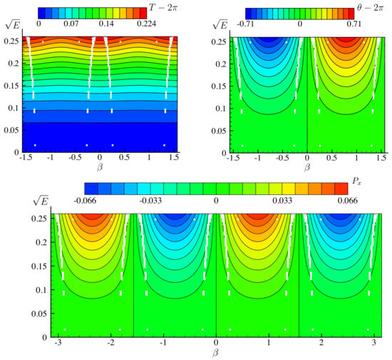
Figure 4. Dependence of the temporal period, T, spatial phase shift, $\theta$, and momentum, $P_x$, on amplitude $\epsilon =\sqrt{E}$ and traveling parameter $\beta$. White regions consist of grid cells in the $\beta$-$\epsilon$ mesh for which a solution could not be found at one of the four corner nodes of the cell. Our criterion for finding solutions is that the objective function f in (33) of Section 3.2 is reduced below ${10}^{-26}$.

4.1. Gaps and Disconnections in the Two-Parameter Family

The period, T, spatial phase shift, $\theta$, and momentum, $P_x$, appear to depend smoothly on E and $\beta$ in the contour plots of Figure 4. However, the regular pattern of white grid cells (bordering a gridpoint where a solution could not be found) suggest the presence of discontinuities running through the two-parameter family of traveling-standing waves. A useful variable for studying these discontinuities and visualizing the shape of the waves is the signed curvature at the origin at $t=0$,

$$\kappa =-\frac{{\eta }_{xx}(0,0)}{{\left(1+{\eta }_x{(0,0)}^2\right)}^{3/2}}=-{\eta }_{xx}(0,0),$$

(54)

where we used (17). A contour plot of $\kappa$ versus energy and traveling parameter is shown in Figure 5. The spacing of contour lines is highly non-uniform to avoid having large regions of the graph with no contour lines and other regions where the contour lines are so dense that they become indistinguishable (the plot actually shows $arcsinh\left(5\kappa \right)$, but the labels on the colorbar correspond to $\kappa$). The curvature is much larger when E is large and $\beta$ is close to zero than elsewhere in the plot. This is expected as values of $\beta$ far from 0 (modulo $2\pi$) correspond to solutions in which the largest wave crest over the time interval $0\le t\le T/4$ forms at $(x,t)=(\theta /4,T/4)$ or $(\pi ,0)$ instead of at $(0,0)$. For example, plots A–G in Figure 2 above correspond to $\sqrt{E}=0.25$, $\beta =l\pi /12$, $0\le l\le 6$. The highest wave crests occur at $x=0$, $t=0$ for solutions A–D, and at $x=\theta /4$, $t=T/4$ for solutions D–G. The traveling wave D is the transition point where the wave crest at $(0,0)$ is identical to the one at $(\theta /4,T/4)$.

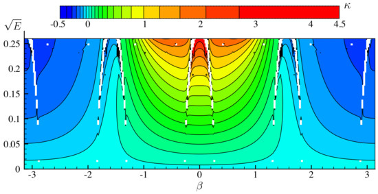
Figure 5. Dependence of the signed curvature $\kappa =-{\eta }_{xx}(0,0)$ on energy E and traveling parameter $\beta$. With the help of Table 1, this plot can be used to determine the curvature of $\eta$ at $x=0$ and $x=\pi$ when $t=0$ as well as at $x=\theta /4$ and $x=\pi +\theta /4$ when $t=T/4$.

Unlike T, $\theta$, and $P_x$, the contour lines of $\kappa$ in Figure 5 veer apart as they approach the white regions from opposite sides. These discontinuities are more easily visualized with graphs than with contour plots. In Figure 6, we show the dependence of $\kappa$ on $\beta$ for 14 fixed values of the amplitude, $\epsilon =\sqrt{E}=0.02\nu$, $0\le \nu \le 13$. For small $\epsilon$, the curvature depends on $\beta$ as $\kappa \approx 2\epsilon cos\beta$, consistent with (25). However as $\epsilon$ increases, $\kappa$ grows rapidly near $\beta =0$, and several disconnections can be seen in the curves. The white regions in Figure 5 occur when a grid point $({\epsilon }_{\nu },{\beta }_l)$ from (51) falls in a gap between disconnections, where no solution exists. These gaps are often narrow enough to cross through the middle of a grid cell without causing the algorithm to fail at the four corner nodes. In this case, the cell will not be white, but contour lines passing through the cell may exhibit sharp kinks. The small but abrupt jumps in some of the contour lines of Figure 5 indicate this type of behavior. Thus, even though most of the white grid cells in Figure 5 border nodes with $\epsilon \ge 0.09$, the eight major disconnections appear to persist all the way down to $\epsilon =0$, where $\beta \in \{\pm \pi /12,\pm 5\pi /12,\pm 7\pi /12,\pm 11\pi /12\}$. We will investigate this in more detail below.

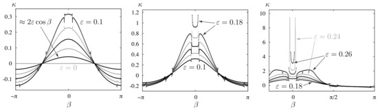
Figure 6. Slices through the contour plot of Figure 5 with $\epsilon =\sqrt{E}=0.02\nu$, $0\le \nu \le 13$. The curvature jumps discontinuously as $\beta$ crosses certain critical values, leaving gaps in the $\beta$-$\epsilon$ parameterization where no solutions exist. When $\epsilon$ is large, the wave crest sharpens rapidly soon after $\beta$ leaves zero in either direction due to a nearby discontinuity on each side.

4.2. Larger-Amplitude Traveling-Standing Water Waves

While the grid spacing in (51) is sufficient to make informative contour plots, the curves in the right panel of Figure 6 are not well-resolved near the disconnections. In Figure 7, we use an adaptive numerical continuation algorithm [12,13] to track solutions with two larger values of energy, $E={\left(0.2683903779\right)}^2$ and $E={\left(0.274\right)}^2$. The former is the energy of the standing wave labeled Y in Figure 10 of [13], which we happened to be studying when we realized that one of the two Jordan chains of the monodromy operator of the linearization about a standing wave should point to standing waves that travel. Surprisingly, the paths bifurcating from standing waves ($\beta =0$) at these two energy levels (green and red in the figure) loop back and meet another standing wave, rather than connecting with a traveling wave. This is very different behavior than what occurs for the Benjamin–Ono equation [18,19], where varying the amplitude of the waves on a path does not affect which stationary or traveling waves it meets at its endpoints, nor the smoothness of the path. However for the free-surface Euler equations, the bifurcation curves become less regular as the amplitude increases. Increasing the energy causes many disconnections to nucleate, leaving gaps in $\beta$ where no solution exists and other regions where multiple solutions exist. Such nucleation events are explored in the context of pure standing waves in [13].

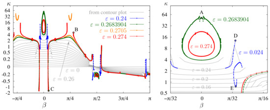
Figure 7. Slices through the contour plot of Figure 5 (grey) along with several additional energy levels in the “extreme” traveling-standing wave regime. Points have also been added to the $\epsilon =0.24$ curve to reveal an imperfect pitchfork bifurcation (blue) where only a spike was seen with the resolution of the contour plot grid (grey). Solutions labeled A–E are plotted in Figures 9 and 10.

The reason it is possible to loop back and connect with a different standing wave is that energy is not a monotonic function as one moves along the family of pure standing waves. The same is true of pure traveling waves, as shown in Figure 8. For standing waves, we plot $\epsilon =\sqrt{E}$ as a function of crest acceleration [7], defined as the acceleration of a fluid particle at the wave crest at the moment it reaches maximum height. For traveling waves, we plot $\epsilon$ as a function of relative crest velocity [53], defined as the velocity of a fluid particle at the wave crest in the frame moving alongside the wave. We note that $A_c$ is close to zero for small-amplitude standing waves and increases toward 1 as the wave crest sharpens, while q is close to 1 for small-amplitude traveling waves and decreases to zero as the wave crest sharpens. Longuett–Higgins and Fox showed that as $q\to 0$, the crest of the traveling wave approaches 120${}^{\circ }$ in a self-similar fashion [53,54]. Penney and Price [3] conjectured a 90${}^{\circ }$ crest angle for the limiting standing wave of the greatest height [3,55,56,57]. Early numerical studies suggested that a sharper corner [7] or a cusp [9] may form as $A_c\to 1$. Recent high-resolution computations show that resonance causes self-similarity at the crest to break down, which prevents a limiting standing wave from materializing at all [12].

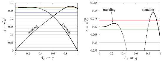
Figure 8. Plots of energy versus crest acceleration $A_c$ (standing waves) or relative crest velocity q (traveling waves). Both curves reach a turning point where E achieves a local maximum. The horizontal lines represent the energy levels of the curves in Figure 7.

Of interest here, in Figure 8, is that the energy levels $\epsilon =0.2684$ (green) and $\epsilon =0.274$ (red) cross the standing-wave curve twice, and these two pure standing waves are connected by (fragmented) closed loops of traveling-standing waves in Figure 7. The $\epsilon =0.2684$ energy level meets the traveling family only once, and indeed the green curve behaves similarly to the grey curves at lower energies near $\beta =\pi /4$ in Figure 7. The $\epsilon =0.274$ energy level does not intersect the traveling wave curve at all in Figure 8, and we see that the red curve in Figure 7 veers upward before reaching $\beta =\pi /4$ from either side, suggesting a sharpening of the wave crest. The intermediate energy level $\epsilon =0.2705$ shown in orange in Figure 8 meets the traveling wave curve in two locations. One wonders whether these are also connected by a path of traveling-standing waves. However, in Figure 7, the orange curves bifurcating from traveling waves at $\beta =\pi /4$ veer away from each other rather than forming a closed loop as in the standing-wave case (aside from small disconnections). The upper orange branch ($\epsilon =0.2705$) veers upward on the $\kappa$ axis, indicating that the crest sharpens as $|\beta -\pi /4|$ increases.

In Figure 9, we show snapshots of the “extreme” waves labeled A, B, and C in Figure 7. Solution A is a pure standing wave with crest acceleration $A_c=0.98$ and curvature $\kappa =51.893$. Solution B ($\beta =0.2804\pi$) is the sharpest traveling-standing wave we computed on the red branch ($\epsilon =0.274$), which has $\kappa =5.068$ at $t=0$ and $\kappa =15.04$ at $t=T/4$. While the crests of many of these traveling-standing waves become quite sharp, analogy with the pure standing-wave case suggests that resonance will prevent a perfect corner from forming when true dynamics are involved, i.e., other than the ${120}^{\circ }$ corner of the highest pure traveling wave [53,54], which can be formulated as a steady-state problem. Solution C in Figure 9 shows a traveling-standing wave with negative curvature due to the formation of a dimple at the wave crest. Referring back to Figure 6, there is a strong discontinuity running through the family of traveling-standing waves to the right of $\beta =0$ in which curvature sharpens when the discontinuity is approached from the left and flattens when approached from the right. At the energy level of the red curve ($\epsilon =0.274$) in Figure 7, the sharpening branch loops back to join another standing wave while the flattening branch acquires negative curvature.

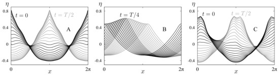
Figure 9. Large-amplitude traveling-standing waves can form relatively sharp wave crests (A,B) with high curvature $\kappa$, or dimpled wave crests (C) with negative curvature $\kappa$. These solutions are also labeled in the bifurcation diagram of Figure 7.

In standing-wave studies [13,39], disconnections in the bifurcation diagrams can often be associated with harmonic resonance between Fourier modes. More generally, disconnections occur when a large-scale carrier wave excites a higher-frequency secondary wave that can be superimposed nonlinearly with one of two amplitudes to make a globally time-periodic solution [12,13]. Figure 10 shows solutions D and E on two branches that meet at an imperfect pitchfork bifurcation at energy level $\epsilon =0.24$ (blue) in Figure 7. The two waves evolve similarly in the large, although a secondary wave on the surface sharpens the crest at D and flattens it at E. In the right panel of Figure 10, we plot the difference between solutions D and E at corresponding times $kT/48$, $0\le k\le 48$. These times are slightly different for the two solutions since $T=6.473269$ for solution D and $T=6.473250$ for solution E. Instead of resembling another standing wave (as happens in the pure standing case), the secondary wave takes the form of a frequency- and amplitude-modulated traveling wave evolving over the surface of a bulk traveling-standing wave.

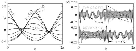
Figure 10. The solutions labeled D and E in Figure 7 behave similarly in the large, differing by a higher-frequency secondary wave responsible for the imperfect pitchfork bifurcation in Figure 7. This secondary wave takes the form of a frequency- and amplitude-modulated traveling wave that either sharpens the wave crest (D) or flattens it (E), depending on the relative phase of the primary and secondary waves.

5. Asymptotic Expansions and Alternative Parameterizations of TS-Waves

We now return to the question of persistence of disconnections to zero-amplitude. We saw above in Figure 5 and Figure 6 that eight major disconnections exist in the $\beta$–$\epsilon$ plane that lead to jumps in curvature when they are crossed and leave gaps where no solution could be found. We have not attempted to derive a formal asymptotic expansion along the lines of Rayleigh [2], Penney and Price [3], Tadjbakhsh and Keller [58], Concus [59], Schwartz and Whitney [5], or Amick and Toland [60]. This is quite challenging even for pure standing waves due to resonant modes of the form $e^{i{m}^{2}x}{e}^{imt}$ and $m\in \mathbb{Z}$, whose amplitudes are determined by compatibility conditions at higher order rather than by remainders from lower-order terms that must be eliminated at the current order. In the pure standing wave case, these asymptotic expansions involve trigonometric polynomials with rational or integer coefficients [5,60]. Assuming the same is true for traveling-standing waves allows us to obtain the formulas through fourth order by fitting numerical data. We first study the asymptotic behavior of the initial conditions, which is natural in a shooting context and involves fewer expansion variables. We then compute the asymptotic expansion of the torus function $\tilde{Z}({\theta }_1,{\theta }_2)$ from Section 3.3 in powers of the amplitude parameter $\epsilon$, which describes both the spatial and temporal behavior of traveling-standing water waves. Finally, we discuss alternative amplitude and traveling parameters and the relative merits of each choice.

5.1. Asymptotic Expansion of the Initial Condition

The numerical data we use to study small-amplitude solutions is plotted in Figure 11. It consists of the first four Fourier modes ${\widehat{\eta }}_j(0;{\epsilon }_{\nu },{\beta }_l)$, ${\widehat{\phi }}_j(0;{\epsilon }_{\nu },{\beta }_l)$ of the initial conditions of the first 21 energy levels ${\epsilon }_{\nu }$ in (51), indexed $0\le \nu \le 20$. For $\beta$, we use ${\beta }_l=\pi l/180$, $l=45,46,\cdots ,90$, and then extend by symmetry to $-180\le l\le 180$. Since we expect a discontinuity at $l=75$, we drop this index from the list and replace it with $l=74.5$ and $l=75.5$. This is also done at all the symmetric images of $l=75$ under the transformation rules of Table 1, leaving 8 gaps in the plots. At each ${\beta }_l$, we approximate each variable of interest by the 10th degree polynomial $p_l\left(\epsilon \right)$ that most nearly agrees with it (in the least-squares sense) at the ${\epsilon }_{\nu }$, $\nu =0,\cdots ,20$. We then evaluate $p_l^{\left(r\right)}\left(0\right)$, $0\le r\le 4$, to obtain the first five Taylor coefficients of the variable. We also do this for the period, $T({\epsilon }_{\nu },{\beta }_l)$, and spatial shift, $\theta ({\epsilon }_{\nu },{\beta }_l)$. Studying plots of the Taylor coefficients as functions of $\beta$, we are able to guess analytic formulas that agree with the numerical data to as many digits as we can compute in double-precision, which varies from 5 to 15 depending on how many derivatives have been taken. The resulting formulas are reported in Table 2.

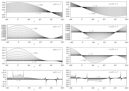
Figure 11. Leading Fourier modes of the initial wave profile, ${\left\{{\widehat{\eta }}_j(0;\epsilon ,\beta )\right\}}_{j=1}^4$, (left), and initial surface velocity potential, ${\left\{{\widehat{\phi }}_j(0;\epsilon ,\beta )\right\}}_{j=1}^4$, (right), versus $\beta$ for small-amplitude traveling-standing waves of amplitude ${\epsilon }_{\nu }=0.002\nu$, $0\le \nu \le 20$. These numerical results were used to guess analytic formulas for the asymptotic expansions, see Table 2. Both ${\widehat{\eta }}_4(0;\epsilon ,\beta )$ and ${\widehat{\phi }}_4(0;\epsilon ,\beta )$ have disconnections at $\beta =\{\pm \frac{\pi }{12},\pm \frac{5\pi }{12},\pm \frac{7\pi }{12},\pm \frac{11\pi }{12}\}$, where the corresponding analytic formulas are singular.

Table 2. Fourth order asymptotic expansion of the initial conditions, period, and phase shift of traveling-standing waves on deep water. Higher-frequency modes are zero through fourth order in $\epsilon =\sqrt{E}$, and ${\widehat{\eta }}_{-j}={\widehat{\eta }}_j$, ${\widehat{\phi }}_{-j}=-{\widehat{\phi }}_j$. We enumerate these functions in the order listed here to define $f_m(\epsilon ,\beta )$ in (57) for $1\le m\le 10$.

$T(\epsilon ,\beta )$	$=2\pi \left[1+\frac{1}{2}{\epsilon }^2+\left(\frac{3}{32}+\frac{15}{32}cos4\beta \right){\epsilon }^4+O\left({\epsilon }^6\right)\right],$
$\theta (\epsilon ,\beta )$	$=2\pi \left[1+\left(\frac{3}{2}sin2\beta \right){\epsilon }^2+\left(\frac{9}{8}sin2\beta \right){\epsilon }^4+O\left({\epsilon }^6\right)\right],$
${\widehat{\eta }}_1(0;\epsilon ,\beta )$	$=\epsilon cos\beta -\frac{1}{2}{\epsilon }^{3}cos\beta +O\left({\epsilon }^5\right),$
$-i{\widehat{\phi }}_1(0;\epsilon ,\beta )$	$=-\epsilon sin\beta +{\epsilon }^{3}sin2\beta cos\beta +O\left({\epsilon }^5\right),$
${\widehat{\eta }}_2(0;\epsilon ,\beta )$	$={\epsilon }^2{cos}^2\beta -\left(\frac{11}{21}cos2\beta +\frac{31}{24}cos4\beta +\frac{3}{8}\right){\epsilon }^4+O\left({\epsilon }^6\right),$
$-i{\widehat{\phi }}_2(0;\epsilon ,\beta )$	$=-\frac{1}{2}{\epsilon }^{2}sin2\beta +\left(\frac{29}{42}sin4\beta -\frac{1}{12}sin2\beta \right){\epsilon }^4+O\left({\epsilon }^6\right),$
${\widehat{\eta }}_3(0;\epsilon ,\beta )$	$=\frac{3}{2}{\epsilon }^3{cos}^3\beta +O\left({\epsilon }^5\right),$         $-i{\widehat{\phi }}_3(0;\epsilon ,\beta )=-\frac{3}{2}{\epsilon }^{3}sin\beta {cos}^2\beta +O\left({\epsilon }^5\right),$
${\widehat{\eta }}_4(0;\epsilon ,\beta )$	$=\left(\frac{(5/96)cos2\beta }{{cos}^{2}2\beta -3/4}+\frac{1+62{cos}^4\beta }{24}-\frac{{sin}^{2}2\beta }{48}\right){\epsilon }^4+O\left({\epsilon }^6\right),$
$-i{\widehat{\phi }}_4(0;\epsilon ,\beta )$	$=\left(\frac{(5/192)sin4\beta }{{cos}^{2}2\beta -3/4}-\frac{2}{3}sin2\beta -\frac{13}{48}sin4\beta \right){\epsilon }^4+O\left({\epsilon }^6\right).$

Since fourth derivatives lead to a significant cancellation of digits, we verify the results by re-computing the solutions in quadruple-precision on a 33-point Chebyshev–Lobatto grid in the amplitude parameter over the interval $-0.032\le \epsilon \le 0.032$,

$${\epsilon }_{\nu }=0.032cos\left(\pi (16-\nu )/32\right),-16\le \nu \le 16.$$

(55)

The traveling-standing wave calculations are only performed for $1\le \nu \le 16$, i.e., for ${\epsilon }_{\nu }>0$. Further details on these quadruple-precision calculations will be given in Section 5.2 below. We use the $\epsilon =0$ values of the formulas in Table 2 at $\nu =0$ and use even or odd symmetry of these formulas with respect to $\epsilon$ for $\nu <0$:

$$\begin{array}{cc}\hfill {\widehat{\eta }}_j(0;{\epsilon }_{-\nu },{\beta }_l)& ={(-1)}^j{\widehat{\eta }}_j(0;{\epsilon }_{\nu },{\beta }_l),\hfill \\ \hfill {\widehat{\phi }}_j(0;{\epsilon }_{-\nu },{\beta }_l)& ={(-1)}^j{\widehat{\phi }}_j(0;{\epsilon }_{\nu },{\beta }_l),\hfill \end{array}\begin{array}{cc}\hfill T({\epsilon }_{-\nu },{\beta }_l)& =T({\epsilon }_{\nu },{\beta }_l),\hfill \\ \hfill \theta ({\epsilon }_{-\nu },{\beta }_l)& =\theta ({\epsilon }_{\nu },{\beta }_l),\hfill \end{array}(1\le \nu \le 16).$$

(56)

As shown in the left panel of Figure 12, the Chebyshev modes of the interpolated functions decay exponentially rather than algebraically, which is strong evidence that the analytic continuation to $\epsilon <0$ for each of these functions is correct. The choice of a 33-point Chebyshev–Lobatto grid and the parameter 0.032 in (55) were chosen by trial and error to ensure that the Chebyshev modes of these functions decay to quadruple-precision accuracy using polynomials of a degree ≤32.

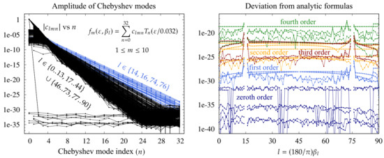
Figure 12. Verification in quadruple-precision of the proposed asymptotic expansions of Table 2. (left) Chebyshev mode amplitudes $|c_{lmn}|$ of the interpolating polynomials $f_m^{\mathrm{interp}}(\epsilon ,{\beta }_l)$ for different choices of m and l. (right) Plots of $|a_{lm}^{\left(r\right)}-{\alpha }_m^{\left(r\right)}\left({\beta }_l\right)|$ versus l comparing the analytic formulas in Table 2 to the expansion obtained numerically from $f_{lm}^{\mathrm{interp}}\left(\epsilon \right)$. These curves correspond to the variables listed in Table 3 at each order $r\in \{0,1,2,3,4\}$.

We introduce additional notation to enumerate the functions listed in Table 2 to facilitate the discussion of the numerical results reported in Figure 12:

$$\begin{array}{cc}\hfill f_1(\epsilon ,\beta )& =T(\epsilon ,\beta ),\hfill \\ \hfill f_2(\epsilon ,\beta )& =\theta (\epsilon ,\beta ),\hfill \\ \hfill f_{2j+1}(\epsilon ,\beta )& ={\widehat{\eta }}_j(0;\epsilon ,\beta ),\hfill & \hfill 1& \le j\le 4,\hfill \\ \hfill f_{2j+2}(\epsilon ,\beta )& =-i{\widehat{\phi }}_j(0;\epsilon ,\beta ),\hfill & \hfill 1& \le j\le 4.\hfill \end{array}$$

(57)

The Fourier modes of the velocity potential at $t=0$ are purely imaginary due to (17), so $f_{2j+2}$ extracts the imaginary part of ${\widehat{\phi }}_j(0;\epsilon ,\beta )$. Each function $f_m(\epsilon ,{\beta }_l)$ is sampled on the Chebyshev grid (55), where ${\beta }_l=\pi l/180$ with l ranging over the integers between 0 and 90, excluding 15, 45, and 75. We omit $l=45$ to avoid the special treatment required for traveling waves discussed at the beginning of Section 4. The interpolating polynomial:

$$f_{lm}^{\mathrm{interp}}\left(\epsilon \right)=\sum _{n=0}^{32}{c}_{lmn}{T}_n(\epsilon /0.032)$$

(58)

is then constructed using the Fast Fourier Transform to compute the Chebyshev coefficients $c_{lmn}$ from the sampled values, $f_m({\epsilon }_{\nu },{\beta }_l)$. The $|c_{lmn}|$ are plotted versus n in the left panel of Figure 12. The plot contains 880 curves corresponding to the different choices of l and m, all of which decay below ${10}^{-27}$ by the time the Chebyshev mode index reaches 32. Every other Chebyshev mode on each curve is zero, with parity depending on whether we use even or odd symmetry to extend the sampled values $f_m({\epsilon }_{\nu },{\beta }_l)$ to ${\epsilon }_{\nu }<0$ in (56). In the plot, we omit the Chebyshev modes $|c_{lmn}|$ that are zero by symmetry. The curves with the slowest decay rate, plotted in blue in the figure, correspond to ${\beta }_l$ with $l\in \{14,16,74,76\}$. This occurs because the asymptotic expansion breaks down as $\beta$ approaches ${15}^{\circ }$ and ${75}^{\circ }$ due to the presence of $({cos}^{2}2\beta -3/4)$ in the denominators of ${\widehat{\eta }}_4(0;\epsilon ,\beta )$ and ${\widehat{\phi }}_4(0;\epsilon ,\beta )$ in Table 2. Thus, the functions $f_m(\epsilon ,\beta )$ vary more rapidly with $\epsilon$ as $\beta$ approaches these values. One would need to use a smaller prefactor than $0.032$ in (55) or increase the number of Chebyshev modes to maintain quadruple-precision accuracy for $\beta$ closer to ${15}^{\circ }$ or ${75}^{\circ }$ than reported here.

For each function $f_m(\epsilon ,\beta )$, we fit the data from the double-precision calculations to obtain an ansatz for the analytic form of the leading terms in the expansion:

$$f_m(\epsilon ,\beta )={\alpha }_m^{\left(0\right)}\left(\beta \right)+\epsilon {\alpha }_m^{\left(1\right)}\left(\beta \right)+{\epsilon }^2{\alpha }_m^{\left(2\right)}\left(\beta \right)+{\epsilon }^3{\alpha }_m^{\left(3\right)}\left(\beta \right)+{\epsilon }^4{\alpha }_m^{\left(4\right)}\left(\beta \right)+\cdots .$$

(59)

The results are reported in Table 2. For example, $m=4$ corresponds to $f_4(\epsilon ,\beta )=-i{\widehat{\phi }}_1(0;\epsilon ,\beta )$, so:

$${\alpha }_4^{\left(1\right)}\left(\beta \right)=-sin\beta ,{\alpha }_4^{\left(3\right)}\left(\beta \right)=sin2\beta cos\beta ,{\alpha }_4^{\left(r\right)}\left(\beta \right)=0(r=0,2,4).$$

(60)

We compare these analytic formulas to the coefficients in the expansion of the interpolating polynomial:

$$f_{lm}^{\mathrm{interp}}\left(\epsilon \right)=a_{lm}^{\left(0\right)}+\epsilon a_{lm}^{\left(1\right)}+{\epsilon }^2{a}_{lm}^{\left(2\right)}+{\epsilon }^3{a}_{lm}^{\left(3\right)}+{\epsilon }^4{a}_{lm}^{\left(4\right)}+\cdots ,$$

(61)

which are easily expressed in terms of the Chebyshev modes $c_{lmn}$ of (58),

$$\begin{array}{cc}\hfill a_{lm}^{\left(0\right)}& =\sum _{n\mathrm{even}}{(-1)}^{n/2}{c}_{lmn},a_{lm}^{\left(1\right)}=\frac{1}{0.032}\sum _{n\mathrm{odd}}n{(-1)}^{(n-1)/2}{c}_{lmn},\hfill \\ \hfill a_{lm}^{\left(2\right)}& =\frac{1}{{\left(0.032\right)}^2}\sum _{n\mathrm{even}}\frac{n^2}{2}{(-1)}^{(n-2)/2}{c}_{lmn},\hfill \\ \hfill a_{lm}^{\left(3\right)}& =\frac{1}{{\left(0.032\right)}^3}\sum _{n\mathrm{odd}}\frac{(n^2-1)(2n+1)}{6}{(-1)}^{(n-3)/2}{c}_{lmn},\hfill \\ \hfill a_{lm}^{\left(4\right)}& =\frac{1}{{\left(0.032\right)}^4}\sum _{n\mathrm{even}}\frac{(n^2-4)n^2}{24}{(-1)}^{(n-4)/2}{c}_{lmn}.\hfill \end{array}$$

(62)

When computing $a_{lm}^{\left(r\right)}$, the first nonzero entry in the sum is $n=r$, and the sum is over integers n in the range $r\le n\le 32$ such that $(n-r)$ is even.

The results of this comparison are shown in the right panel of Figure 12. We plot the deviation $e_{lm}^{\left(r\right)}=|a_{lm}^{\left(r\right)}-{\alpha }_m^{\left(r\right)}\left({\beta }_l\right)|$ of the expansion coefficients obtained numerically from the interpolating polynomial to the proposed exact formulas in Table 2. The curves are color coded and labeled by the order r of $e_{lm}^{\left(r\right)}$. The errors $e_{lm}^{\left(r\right)}$ generally increase with r, which is expected due to the growing prefactor $1/{\left(0.032\right)}^r$ and increasing powers of n in the formulas (62) for $a_{lm}^{\left(r\right)}$. In particular, an error of order ${10}^{-30}$ in $c_{lmn}$ with $n=32$ is amplified by a factor of $({32}^2-4)\left({32}^2\right){\left(0.032\right)}^{-4}/24=4.2\times {10}^{10}.$ In these plots, l ranges from 0 to 90 omitting 15, 45, and 75 and m and r range over the marked entries of Table 3. Solid markers in the table correspond to nonzero formulas for ${\alpha }_m^{\left(r\right)}\left(\beta \right)$ in Table 2. For example, from (60), the $m=4$ column has solid markers in rows $r=1$ and $r=3$, thus, the curves $e_{l4}^{\left(1\right)}$ and $e_{l4}^{\left(3\right)}$ are among those plotted in the right panel of Figure 12 and labeled ‘first order’ and ‘third order,’ respectively. Open markers in Table 3 correspond to coefficients $a_{lm}^{\left(r\right)}$ for which there are nonzero coefficients $c_{lmn}$ in the right-hand side of (62) that must cancel to yield zero, which is the value of ${\alpha }_m^{\left(r\right)}\left({\beta }_l\right)$ in these cases. For example, the open marker at $r=1$, $m=7$ corresponds to one of the four curves labeled ‘first order’ in Figure 12, which is a plot of $e_{l7}^{\left(1\right)}=\left|a_{l7}^{\left(1\right)}\right|$. Blank entries in Table 3 correspond to entries $a_{lm}^{\left(r\right)}$ that are zero due to symmetry, i.e., the sums in the right-hand side of (62) involve only $c_{lmn}$ entries that are zero due to the even or odd extension that was used to compute $f_m({\epsilon }_{\nu },{\beta }_l)$ for ${\epsilon }_{\nu }<0$. These entries are not plotted in Figure 12 since the error is exactly zero.

Table 3. Indices m and r of the error curves $|a_{lm}^{\left(r\right)}-{\alpha }_m^{\left(r\right)}\left({\beta }_l\right)|$ plotted in the right panel of Figure 12. Solid markers denote indices for which the proposed exact formulas ${\alpha }_m^{\left(r\right)}\left(\beta \right)$ in Table 2 are nonzero while open markers denote entries where nonzero terms $c_{lmn}$ have to cancel in the sums (62) to achieve $a_{lm}^{\left(r\right)}\approx {\alpha }_m^{\left(r\right)}\left({\beta }_l\right)=0$.

m:	1	2	3	4	5	6	7	8	9	10
variable:	T	$\mathit{\theta }$	${\widehat{\mathit{\eta }}}_1$	${\widehat{\mathit{\phi }}}_1$	${\widehat{\mathit{\eta }}}_2$	${\widehat{\mathit{\phi }}}_2$	${\widehat{\mathit{\eta }}}_3$	${\widehat{\mathit{\phi }}}_3$	${\widehat{\mathit{\eta }}}_4$	${\widehat{\mathit{\phi }}}_4$
$r=0$	•	•			∘	∘			∘	∘
$r=1$			•	•			∘	∘
$r=2$	•	•			•	•			∘	∘
$r=3$			•	•			•	•
$r=4$	•	•			•	•			•	•

Since the errors $e_{lm}^{\left(r\right)}$ computed in quadruple-precision and plotted in Figure 12 are 12–16 orders of magnitude smaller than those of the double-precision calculations that were used to discern the analytic formulas of Table 2, we are confident that these formulas are correct. We find that the disconnections in the plots of ${\widehat{\eta }}_4(0;\epsilon ,\beta )$ and ${\widehat{\phi }}_4(0;\epsilon ,\beta )$ in Figure 11 are cleanly represented at fourth order by the terms with $({cos}^{2}2\beta -3/4)$ in the denominator in Table 2. This shows that the disconnections do indeed persist all the way to zero-amplitude, where they manifest as terms in the asymptotic expansion of the Fourier coefficients that diverge as $\beta$ approaches $\{\pm \frac{\pi }{12},\pm \frac{5\pi }{12},\pm \frac{7\pi }{12},\pm \frac{11\pi }{12}\}$. The fact that the formulas for ${\widehat{\eta }}_j(0;\epsilon ,\beta )$ and ${\widehat{\phi }}_j(0;\epsilon ,\beta )$ can be expanded in integer powers of $\epsilon$ with coefficients that involve only trigonometric polynomials of $\beta$ confirms that defining $\epsilon =\sqrt{E}$ and $\beta$ via (23) were good choices for the amplitude and traveling parameters.

5.2. Asymptotic Expansion of the Solution on the Rotated Torus

Using the numerical solutions computed in quadruple-precision to verify the ansatz of Table 2 for the asymptotic expansion of the initial conditions, we are able to identify exact formulas for the leading terms in the asymptotic expansion of the 2D Fourier coefficients of the torus function $\tilde{Z}({\theta }_1,{\theta }_2)$ described in Section 3.3. For each amplitude ${\epsilon }_{\nu }$ in (55) in the range $1\le \nu \le 16$ and ${\beta }_l=\pi l/180$ with l ranging over the integers between 0 and 90, omitting 15, 45, and 75, we compute a traveling-standing wave with $M=128$ gridpoints in space and 32 timesteps taken from 0 to $T/4$ using a 15th order spectral deferred correction method [44,45,46] based on the Gauss–Lobatto quadrature. For each ${\epsilon }_{\nu }$, we use the following cutoff beyond which the Fourier modes of the initial condition are set to zero in the Levenberg–Marquardt algorithm

$$\begin{array}{cccccccccccc}\hfill \nu & 1& 2& 3& 4& 5& 6& 7& 8& 9& 10& 11–16\\ \hfill N/2& 18& 19& 20& 21& 22& 23& 24& 25& 26& 27& 28\end{array}.$$

These cutoffs are large enough that the Fourier modes ${\widehat{\eta }}_j(0;\epsilon ,\beta )$ and ${\phi }_j(0;\epsilon ,\beta )$ of the initial condition decay below ${10}^{-30}$ by the time j reaches $N/2$. The solver also computes T and $\theta$ as explained in Section 3.2 above. These numerical results fill the rotated rectangle corresponding to $0\le t\le T/4$ in Figure 3 with values of $\tilde{Z}$ on a uniform grid rotated clockwise by ${45}^{\circ }$. We extend these values to the region:

$$0\le {\theta }_1,{\theta }_2\le 2\pi$$

(63)

using the rotational symmetry of (46) (with a sign change in velocity potential) about the three lattice points shown with black markers in Figure 3. Extracting the values of $\tilde{Z}({\theta }_1,{\theta }_2)$ in a checkerboard pattern from the points of the rotated grid that satisfy (63) gives values for $\tilde{Z}({\theta }_1,{\theta }_2)$ on a uniform non-rotated $64\times 64$ grid over ${\mathbb{T}}^2$.

We denote the two components of $\tilde{Z}$ by $\tilde{\eta }({\theta }_1,{\theta }_2;\epsilon ,\beta )$ and $\tilde{\phi }({\theta }_1,{\theta }_2;\epsilon ,\beta )$ and compute the 2D Fourier series coefficients of these functions,

$${\widehat{\eta }}_{j_1,j_2}(\epsilon ,\beta )=\frac{1}{4{\pi }^2}{\int \int }_{{\mathbb{T}}^2}\tilde{\eta }({\theta }_1,{\theta }_2;\epsilon ,\beta )e^{-i{j}_1{\theta }_1}{e}^{-i{j}_2{\theta }_2}d{\theta }_{1}d{\theta }_2,$$

(64)

using the 2D FFT in quadruple-precision to obtain the modes with $max\left(\right|j_1|,|j_2\left|\right)\le 32$ from the values on the $64\times 64$ grid. For each ${\epsilon }_{\nu }$ and ${\beta }_l$ in the ranges described above, we find that $max\left(\right|{\widehat{\eta }}_{j_1,j_2}({\epsilon }_{\nu },{\beta }_l)|,|{\widehat{\phi }}_{j_1,j_2}({\epsilon }_{\nu },{\beta }_l)\left|\right)$ decays below ${10}^{-29}$ for $j_1^2+j_2^2\ge {24}^2$. Since $\tilde{\eta }$ and $\tilde{\phi }$ are real-valued and satisfy the symmetry condition (45),

$${\widehat{\eta }}_{-j_1,-j_2}={\widehat{\eta }}_{j_1,j_2}\in \mathbb{R}\mathrm{and}i{\widehat{\phi }}_{-j_1,-j_2}=-i{\widehat{\phi }}_{j_1,j_2}\in \mathbb{R},(j_1,j_2\in \mathbb{Z}).$$

(65)

In particular, ${\widehat{\phi }}_{00}=0$. In fact, all the modes ${\widehat{\eta }}_{j_1,j_2}$ and ${\widehat{\phi }}_{j_1,j_2}$ with $j_1=j_2$ are zero due to:

$${\int }_0^{2\pi }\eta (x,t)dx=0,{\int }_0^{2\pi }\phi (x,t)dx=0,(t\ge 0).$$

(66)

These integrals are conserved quantities under (2) and are assumed to be zero initially. Making use of periodicity of $\tilde{Z}({\theta }_1,{\theta }_2)$ in Figure 3, the change of variables ${\theta }_1={\omega }_{1}t+x$ and ${\theta }_2={\omega }_{2}t-x$ with ${\omega }_1$ and ${\omega }_2$ as in (43) then gives:

$${\widehat{\eta }}_{j_1,j_1}=\frac{1}{2\pi (T/2)}{\int }_0^{T/2}\left({\int }_{-\pi +(\theta -2\pi )t/T}^{\pi +(\theta -2\pi )t/T}\eta (x,t)dx\right)e^{-i{j}_{1}4\pi t/T}dt=0,$$

(67)

with an identical formula yielding ${\widehat{\phi }}_{j_1,j_1}=0$, as claimed.

We analytically continue ${\widehat{\eta }}_{j_1,j_2}(\epsilon ,{\beta }_l)$ and ${\widehat{\phi }}_{j_1,j_2}(\epsilon ,{\beta }_l)$ to $\epsilon <0$ as even or odd functions of $\epsilon$, depending on whether $j_1+j_2$ is even or odd. We expect the leading term of the asymptotic expansions of ${\widehat{\eta }}_{j_1,j_2}(\epsilon ,{\beta }_l)$ and ${\widehat{\phi }}_{j_1,j_2}(\epsilon ,{\beta }_l)$ to be at most $O\left({\epsilon }^{|j_1|+|j_2|}\right)$, which we confirm for $|j_1|+|j_2|\le 5$. To this end, we enumerate these modes by:

$$f_m(\epsilon ,\beta )=\left\{\begin{array}{cc}{\widehat{\eta }}_{j_1,j_2}(\epsilon ,\beta ),& m\mathrm{odd}\\ {\widehat{\phi }}_{j_1,j_2}(\epsilon ,\beta ),& m\mathrm{even}\end{array}\right\},(1\le m\le 62),$$

(68)

where $j_1$ and $j_2$ depend on m via:

$$\begin{array}{c}\begin{array}{ccccccccccccccccccc}\hfill 2\lceil m/2\rceil & 2& 4& 6& 8& 10& 12& 14& 16& 18& 20& 22& 24& 26& 28& 30& 32& 34& 36\\ \hfill j_1& 0& 1& 0& 1& 2& 3& 2& 1& 0& 1& 2& 3& 4& 5& 4& 3& 2& 1\\ \hfill j_2& 1& 0& 3& 2& 1& 0& -1& -2& 5& 4& 3& 2& 1& 0& -1& -2& -3& -4\end{array}\\ \begin{array}{cccccccccccccc}\hfill 2\lceil m/2\rceil & 38& 40& 42& 44& 46& 48& 50& 52& 54& 56& 58& 60& 62\\ \hfill j_1& 0& 0& 1& 2& 1& 0& 1& 2& 3& 4& 3& 2& 1\\ \hfill j_2& 0& 2& 1& 0& -1& 4& 3& 2& 1& 0& -1& -2& -3\end{array}\end{array}$$

(69)

Note that $2\lceil m/2\rceil$ rounds odd integers up to even integers and leaves even integers unchanged. Thus, if m is odd, the corresponding $(j_1,j_2)$ are the same as for $m+1$ listed in (69). In our numbering, the lattice points corresponding to $m\le 36$ have odd parity ($j_1+j_2$ odd). These are denoted by red circles in Figure 13a. Those with $37\le m\le 62$ have even parity and are denoted by blue squares in the figure. Filled markers denote Fourier lattice points where nonzero terms are present in the fourth order asymptotic expansion of ${\widehat{\eta }}_{j_1,j_2}$ or ${\widehat{\phi }}_{j_1,j_2}$ while open markers denote lattice points where we compute the asymptotic expansion numerically to confirm that the leading terms through fourth order are zero. Grey markers denote lattice points where (65) can be used to determine ${\widehat{\eta }}_{j_1,j_2}$ and ${\widehat{\phi }}_{j_1,j_2}$ from those with blue or red markers.

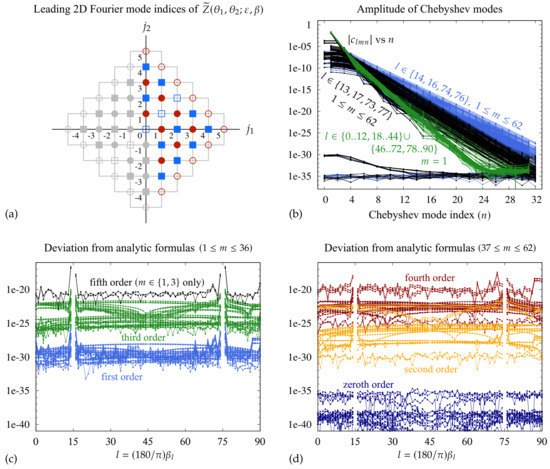
Figure 13. Verification in quadruple-precision of the proposed asymptotic expansions of Table 4 and Table 5. (a) 2D Fourier mode indices where we compute the expansion coefficients. (b) The Chebyshev mode amplitudes $|c_{lmn}|$ of the interpolating polynomials $f_{lm}^{\mathrm{interp}}\left(\epsilon \right)$ in (58) decay exponentially. (c,d) Plots of $|a_{lm}^{\left(r\right)}-{\alpha }_m^{\left(r\right)}\left({\beta }_l\right)|$ versus l comparing the analytic formulas in Table 4 and Table 5 to the expansion obtained numerically from $f_{lm}^{\mathrm{interp}}\left(\epsilon \right)$.

Each of the functions $f_m(\epsilon ,\beta )$ in (68) is evaluated at the points $({\epsilon }_{\nu },{\beta }_l)$ described above and extended by even or odd symmetry to obtain values at ${\epsilon }_{-\nu }$. We compute the Chebyshev representation (58) of the interpolating polynomial $f_{lm}^{\mathrm{interp}}\left(\epsilon \right)$ as before, but m now runs from 1 to 62 instead of 1 to 10 due to the change in meaning of $f_m(\epsilon ,\beta )$ from (57) to (68). Figure 13b shows the exponential decay of these Chebyshev expansion coefficients for a subset of the functions $f_m(\epsilon ,{\beta }_l)$ that were sampled. As in Figure 12, we omit the Chebyshev modes $|c_{lmn}|$ that are zero due to the even or odd symmetry of the analytic continuation; this avoids NaN values at every other point due to the log scale of the y-axis. The blue curves in Figure 13b correspond to $1\le m\le 62$ and $l\in \{14,16,74,76\}$. These are the closest ${\beta }_l$ values to the singularities at $\beta ={15}^{\circ }$ and ${75}^{\circ }$. The black curves correspond to $1\le m\le 62$ and $l\in \{13,17,73,77\}$, which are the next closest points ${\beta }_l$ to the singularities. The green curves show the remaining l values ($0\le l\le 12$, $18\le l\le 44$, $46\le l\le 72$, $78\le l\le 90$), but only for $m=1$, which corresponds to $f_1(\epsilon ,\beta )={\widehat{\eta }}_{01}(\epsilon ,\beta )$. The other choices of m in the range $2\le m\le 62$ for these remaining l values are similar to the $m=1$ case shown, with Chebyshev amplitudes that lie well below most of the black curves. This is strong evidence that all solutions have been resolved by the interpolating polynomial with 27–32 digits of accuracy, with the least accurate approximations corresponding to the four values of ${\beta }_l$ closest to the singularities.

Next we compute the expansion coefficients $a_{lm}^{\left(r\right)}$ of the interpolating polynomial, defined by (61), using (62). We also compute the fifth-order term:

$$a_{lm}^{\left(5\right)}=\frac{1}{{\left(0.032\right)}^5}\sum _{n\mathrm{odd}}\frac{n(n^2-4n+3)(n^2+4n+3)}{120}{(-1)}^{(n-5)/2}{c}_{lmn}$$

(70)

for the cases $m=1$ and $m=3$, which correspond to ${\widehat{\eta }}_{01}$ and ${\widehat{\eta }}_{10}$, respectively. (These fifth order terms are needed in Section 5.3 below). We then look for analytic formulas for the coefficients ${\alpha }_m^{\left(r\right)}\left(\beta \right)$ of (59) that agree closely with the $a_{lm}^{\left(r\right)}$. The results are reported in Table 4 for the Fourier modes with odd parity and in Table 5 for those with even parity. The formulas are simpler when expressed in terms of $\gamma =\beta -\pi /4$ and $\delta =\epsilon /\sqrt{2}$, so we present them this way. We only report formulas for the Fourier modes with filled red or blue markers in Figure 13 since the others are either zero or can be determined from these via (65). In particular, as noted in (67) above, ${\widehat{\eta }}_{j_1,j_2}$ and ${\phi }_{j_1,j_2}$ are zero if $j_1=j_2$ due to conservation of mass and conservation of the mean value of $\phi$ under (2).

Table 4. Asymptotic expansion of the 2D Fourier modes of $\tilde{Z}({\theta }_1,{\theta }_2)$ with odd parity. Here $\delta =\epsilon /\sqrt{2}$ is the expansion parameter and $\gamma =\beta -\pi /4$. We omit modes that we know to be zero, or that can be determined from ${\widehat{\eta }}_{-j_1,-j_2}={\widehat{\eta }}_{j_1,j_2}$ and ${\widehat{\phi }}_{-j_1,-j_2}=-{\widehat{\phi }}_{j_1,j_2}$. $T(\epsilon ,\beta )$ and $\theta (\epsilon ,\beta )$ from Table 2 are easily expressed in terms of $\delta$ and $\gamma$, so we omit them here. An extra order is needed in ${\widehat{\eta }}_{01}$ and ${\widehat{\eta }}_{10}$ to derive (74) below.

${\widehat{\eta }}_{01}$	$=\delta cos\gamma -{\delta }^3{cos}^3\gamma -{\delta }^5\left(\frac{241}{96}cos\gamma +\frac{3041}{1344}cos3\gamma +\frac{2041}{1344}cos5\gamma \right)+O\left({\delta }^7\right),$
${\widehat{\eta }}_{10}$	$=-\delta sin\gamma +{\delta }^3{sin}^3\gamma +{\delta }^5\left(\frac{241}{96}sin\gamma -\frac{3041}{1344}sin3\gamma +\frac{2041}{1344}sin5\gamma \right)+O\left({\delta }^7\right),$
		$-i{\widehat{\phi }}_{01}$	$=\delta cos\gamma -{\delta }^3\left(cos\gamma +cos3\gamma \right)+O\left({\delta }^5\right),$
		$-i{\widehat{\phi }}_{10}$	$=-\delta sin\gamma +{\delta }^3\left(sin\gamma -sin3\gamma \right)+O\left({\delta }^5\right),$
${\widehat{\eta }}_{03}$	$=\frac{3}{2}{\delta }^3{cos}^3\gamma +O\left({\delta }^5\right),$	$-i{\widehat{\phi }}_{03}$	$=\frac{3}{2}{\delta }^3{cos}^3\gamma +O\left({\delta }^5\right),$
${\widehat{\eta }}_{12}$	$=\frac{1}{2}{\delta }^{3}sin2\gamma cos\gamma +O\left({\delta }^5\right),$	$-i{\widehat{\phi }}_{12}$	$=O\left({\delta }^5\right),$
${\widehat{\eta }}_{21}$	$=-\frac{1}{2}{\delta }^{3}sin2\gamma sin\gamma +O\left({\delta }^5\right),$	$-i{\widehat{\phi }}_{21}$	$=O\left({\delta }^5\right),$
${\widehat{\eta }}_{30}$	$=-\frac{3}{2}{\delta }^3{sin}^3\gamma +O\left({\delta }^5\right),$	$-i{\widehat{\phi }}_{30}$	$=-\frac{3}{2}{\delta }^3{sin}^3\gamma +O\left({\delta }^5\right),$
${\widehat{\eta }}_{2,-1}$	$=\frac{9}{4}{\delta }^{3}sin2\gamma sin\gamma +O\left({\delta }^5\right),$	$-i{\widehat{\phi }}_{2,-1}$	$=\frac{3}{8}{\delta }^3\left(cos\gamma -cos3\gamma \right)+O\left({\delta }^5\right),$
${\widehat{\eta }}_{1,-2}$	$=-\frac{9}{4}{\delta }^{3}sin2\gamma cos\gamma +O\left({\delta }^5\right),$	$-i{\widehat{\phi }}_{1,-2}$	$=\frac{3}{8}{\delta }^3\left(sin\gamma +sin3\gamma \right)+O\left({\delta }^5\right).$

Table 5. Fourth order asymptotic expansion of the 2D Fourier modes of $\tilde{Z}({\theta }_1,{\theta }_2)$ with even parity. Here $\delta =\epsilon /\sqrt{2}$ is the expansion parameter and $\gamma =\beta -\pi /4$. The $O\left({\delta }^4\right)$ coefficients of ${\widehat{\eta }}_{j_1,j_2}$ and ${\widehat{\phi }}_{j_1,j_2}$ are singular for $\gamma \in \{\pm \pi /6,\pm 5\pi /6\}$ when $(j_1,j_2)=(3,-1)$ and at $\gamma =\{\pm \pi /3,\pm 4\pi /3\}$ when $(j_1,j_2)=(1,-3)$.

${\widehat{\eta }}_{02}$	$={\delta }^2{cos}^2\gamma +{\delta }^4\frac{31cos2\gamma -20}{3}{cos}^2\gamma +O\left({\delta }^6\right),$	$-i{\widehat{\phi }}_{02}$	$={\delta }^2{cos}^2\gamma +{\delta }^4\frac{8cos2\gamma -7}{3}{cos}^2\gamma +O\left({\delta }^6\right),$
${\widehat{\eta }}_{20}$	$={\delta }^2{sin}^2\gamma -{\delta }^4\frac{31cos2\gamma +20}{3}{sin}^2\gamma +O\left({\delta }^6\right),$	$-i{\widehat{\phi }}_{20}$	$={\delta }^2{sin}^2\gamma -{\delta }^4\frac{8cos2\gamma +7}{3}{sin}^2\gamma +O\left({\delta }^6\right),$
${\widehat{\eta }}_{1,-1}$	$=-{\delta }^{2}sin2\gamma +\frac{1}{2}{\delta }^{4}sin2\gamma +O\left({\delta }^6\right),$	$-i{\widehat{\phi }}_{1,-1}$	$=-\frac{5}{2}{\delta }^{4}sin4\gamma +O\left({\delta }^6\right),$
${\widehat{\eta }}_{0,4}$	$=\frac{8}{3}{\delta }^4{cos}^4\gamma +O\left({\delta }^6\right),$	$-i{\widehat{\phi }}_{0,4}$	$=\frac{8}{3}{\delta }^4{cos}^4\gamma +O\left({\delta }^6\right),$
${\widehat{\eta }}_{1,3}$	$=\frac{67}{21}{\delta }^4{cos}^3\gamma sin\gamma +O\left({\delta }^6\right),$	$-i{\widehat{\phi }}_{1,3}$	$=\frac{22}{21}{\delta }^4{cos}^3\gamma sin\gamma +O\left({\delta }^6\right),$
${\widehat{\eta }}_{3,1}$	$=\frac{67}{21}{\delta }^{4}cos\gamma {sin}^3\gamma +O\left({\delta }^6\right),$	$-i{\widehat{\phi }}_{3,1}$	$=\frac{22}{21}{\delta }^{4}cos\gamma {sin}^3\gamma +O\left({\delta }^6\right),$
${\widehat{\eta }}_{4,0}$	$=\frac{8}{3}{\delta }^4{sin}^4\gamma +O\left({\delta }^6\right),$	$-i{\widehat{\phi }}_{4,0}$	$=\frac{8}{3}{\delta }^4{sin}^4\gamma +O\left({\delta }^6\right),$
${\widehat{\eta }}_{3,-1}$	$={\delta }^4\frac{\left(5cos\gamma -13cos3\gamma \right){sin}^3\gamma }{3cos2\gamma -3/2}+O\left({\delta }^6\right),$	$-i{\widehat{\phi }}_{3,-1}$	$={\delta }^4\frac{\left(5cos\gamma -13cos3\gamma \right){sin}^3\gamma }{6cos2\gamma -3}+O\left({\delta }^6\right),$
${\widehat{\eta }}_{2,-2}$	$=4{\delta }^4{sin}^{2}2\gamma +O\left({\delta }^6\right),$	$-i{\widehat{\phi }}_{2,-2}$	$=O\left({\delta }^6\right),$
${\widehat{\eta }}_{1,-3}$	$=-{\delta }^4\frac{\left(5sin\gamma +13sin3\gamma \right){cos}^3\gamma }{3cos2\gamma +3/2}+O\left({\delta }^6\right),$	$-i{\widehat{\phi }}_{1,-3}$	$={\delta }^4\frac{\left(5sin\gamma +13sin3\gamma \right){cos}^3\gamma }{6cos2\gamma +3}+O\left({\delta }^6\right).$

To systematically identify the analytic formulas reported in Table 4 and Table 5, we begin by assuming:

$${\alpha }_m^{\left(r\right)}\left(\beta \right)d\left(\gamma \right)=[1,cos\gamma ,sin\gamma ,cos\left(2\gamma \right),sin\left(2\gamma \right),\cdots ,cos\left(K\gamma \right),sin\left(K\gamma \right)]\overrightarrow{c},$$

(71)

where $\gamma =\beta -\pi /4$ and $d\left(\gamma \right)=1$ on the first attempt. Here r begins at $|j_1|+|j_2|$ and increases by 2 for successive terms in the expansion, where $(j_1,j_2)$ corresponds to m in (69). We stop at $r=5$ for $m\in \{1,3\}$, at $r=4$ for $m\ge 37$, and at $r=3$ otherwise. We determine $K\ge 1$ and $\overrightarrow{c}=(c_0,c_1,\cdots ,c_{2K})$ by solving the least squares problem $A\overrightarrow{c}=\overrightarrow{a}$, where the lth row of A corresponds to $[1,cos{\gamma }_l,\cdots ,sin\left(K{\gamma }_l\right)]$ with ${\gamma }_l={\beta }_l-\pi /4$, and the lth entry of $\overrightarrow{a}$ is $a_{lm}^{\left(r\right)}\left({\beta }_l\right)d\left({\gamma }_l\right)$. We omit $l\in \{15,45,75\}$ in this enumeration of the equations. We solve this least squares problem in double precision using the values of $a_{lm}^{\left(r\right)}\left({\beta }_l\right)$ computed in quadruple-precision. For all entries except $m\in \{57,58,61,62\}$ and $r=4$, setting $d\left(\gamma \right)=1$ works: The residual of this highly overdetermined system drops suddenly to ${10}^{-15}$ once K reaches r. When $m\in \{57,58,61,62\}$ and $r=4$, we find that with either $d\left(\gamma \right)=6cos2\gamma +3$ or $d\left(\gamma \right)=6cos2\gamma -3$, the residual drops to ${10}^{-15}$ with $K=6$. We then rationalize the floating point numbers in $\overrightarrow{c}$ and simplify the resulting formulas for ${\alpha }_m^{\left(r\right)}\left(\beta \right)$ from (71) to obtain the formulas in Table 4 and Table 5.

As a final check, we compute $e_{lm}^{\left(r\right)}=|a_{lm}^{\left(r\right)}-{\alpha }_m^{\left(r\right)}\left({\beta }_l\right)|$ in quadruple precision using the rational coefficients from Table 4 and Table 5 and plot them versus l in panels (c) and (d) of Figure 13. Panel (c) shows $e_{lm}^{\left(r\right)}$ versus l for $1\le m\le 36$ and $r\in \{1,3\}$. These are the modes ${\widehat{\eta }}_{j_1,j_2}$ and ${\widehat{\phi }}_{j_1,j_2}$ for which odd symmetry is used in the analytic continuation to $\epsilon <0$, which guarantees that $a_{lm}^{\left(r\right)}=0$ for r even. The exponential decay of the Chebyshev modes in panel (b) justifies the use of odd symmetry to extend $f_m(\epsilon ,\beta )$ to $\epsilon <0$. Panel (d) shows $e_{lm}^{\left(r\right)}$ for $37\le m\le 62$ and $r\in \{0,2,4\}$. These are the modes that are extended to $\epsilon <0$ using even symmetry, so it is not necessary to check $r\in \{1,3\}$. We also plot the case of $r=5$ and $m\in \{1,3\}$ in panel (c), which is needed in Section 5.3 below. These curves quantify the loss of precision that occurs for larger values of r due to the powers of ${\left(0.032\right)}^{-r}$ and the $O\left(n^r\right)$ growth of the coefficients in (62) and (70). By performing the calculations in quadruple-precision, we are still able to verify the analytic formulas of Table 4 and Table 5 to at least 19 digits of accuracy. Since only simple fractions appear in the formulas, this is strong evidence that the formulas are correct.

5.3. Alternative Amplitude and Traveling Parameters

One of the main challenges of studying traveling-standing water waves has been to identify suitable amplitude and traveling parameters to describe the two-parameter family. We selected $\epsilon = \sqrt{E}$ and $\beta = atan2\left(e^{i\theta /4}{\widehat{\eta }}_1(T/4),{\widehat{\eta }}_1\left(0\right)\right)$, which leads to nice formulas such as (25) and (27) in the linear regime, and such as given in Table 2, Table 4, and Table 5 when the solutions are expanded in powers of $\epsilon$. These parameters are convenient in a shooting framework as they only depend on the solution at the initial and final times of the required time evolution ($t=0$ and $t=T/4$). At these times, the solution satisfies the symmetry properties (17) and (18), which lead to several transformation rules relating each solution to various phase-shifted or time-reversed versions when $\beta$ is shifted by $\pi$ or reflected about 0 or $\pi /4$.

Another option that may fit better with current methods of proving existence of standing and quasi-periodic water waves [20,21,22,23,24,25,26,27] would be to define new amplitude and traveling parameters, say $\tilde{\delta }$ and $\tilde{\gamma }$, such that the two leading Fourier modes of the $\eta$ component of the torus function $\tilde{Z}({\theta }_1,{\theta }_2)$ satisfy:

$${\widehat{\eta }}_{01}=\tilde{\delta }cos\tilde{\gamma },{\widehat{\eta }}_{10}=-\tilde{\delta }sin\tilde{\gamma }$$

(72)

precisely, without higher-order corrections affecting these two Fourier modes. Substitution of ${\widehat{\eta }}_{01}$ and ${\widehat{\eta }}_{10}$ from Table 4 into:

$$\tilde{\delta }=\delta \sqrt{{({\widehat{\eta }}_{01}/\delta )}^2+{({\widehat{\eta }}_{10}/\delta )}^2},\tilde{\gamma }=\gamma +Im\left\{log\left(e^{-i\gamma }\left[({\widehat{\eta }}_{01}/\delta )-i({\widehat{\eta }}_{10}/\delta )\right]\right)\right\},$$

(73)

we obtain:

$$\begin{array}{cc}\hfill \tilde{\delta }& =\frac{\epsilon }{\sqrt{2}}+\left(-\frac{3}{8}+\frac{1}{8}cos4\beta \right)\frac{{\epsilon }^3}{\sqrt{2}}+O\left({\epsilon }^5\right),\hfill \\ \hfill \tilde{\gamma }& =\left(\beta -\frac{\pi }{4}\right)-\frac{1}{8}\left(sin4\beta \right){\epsilon }^2+\left(-\frac{313}{1344}sin4\beta +\frac{1}{128}sin8\beta \right){\epsilon }^4+O\left({\epsilon }^6\right),\hfill \end{array}$$

(74)

where we used $\delta =\epsilon /\sqrt{2}$ and $\gamma =\beta -\pi /4$. It was necessary to compute ${\widehat{\eta }}_{01}$ and ${\widehat{\eta }}_{10}$ to fifth order in $\delta$ in Table 4 to obtain the fourth-order term for $\tilde{\gamma }$ in (74).

We believe that $\tilde{\delta }$ and $\tilde{\gamma }$ would lead to a qualitatively similar parameterization of the family of traveling-standing waves as our choice of $\epsilon$ and $\beta$. In particular, one can invert (74) to express $\epsilon ,\beta$ and $\delta ,\gamma$ in terms of $\tilde{\delta },\tilde{\gamma }$ in Table 2, Table 4, and Table 5. The coefficients of the new expansions in powers of $\tilde{\delta }$ will still be singular at the fourth order when $\tilde{\gamma }\in \{\pm \frac{\pi }{6},\pm \frac{\pi }{3},\pm \frac{4\pi }{3},\pm \frac{5\pi }{6}\}$, i.e., the disconnections in the two-parameter family of traveling-standing waves do not disappear with different choices of amplitude and traveling parameters. Two additional options would be to focus on $\phi$ instead of $\eta$ and define $\tilde{\delta }$ and $\tilde{\gamma }$ by the requirement that ${\widehat{\phi }}_{01}=i\tilde{\delta }cos\tilde{\gamma }$ and ${\widehat{\phi }}_{10}=-i\tilde{\delta }sin\tilde{\gamma }$ precisely, without higher-order corrections, or to stay within the $\epsilon =\sqrt{E}$ framework and define $\beta = atan2\left(i{\widehat{\phi }}_1\left(0\right),e^{i\theta /4}i{\widehat{\phi }}_1(T/4)\right)$. In each of the four options, the first Fourier modes of $\eta$ and $\phi$ enter at linear order with respect to the amplitude parameter $\epsilon$ or $\tilde{\delta }$, with $\beta$ or $\tilde{\gamma }$ controlling the relative amplitude of the right- and left-traveling waves at linear order, as in (26). At larger amplitudes, each of these parameterizations will describe the same set of traveling-standing waves, just labeled slightly differently. Our choice of $\epsilon ,\beta$ has the advantage that $\epsilon =\sqrt{E}$ has a natural physical interpretation in terms of energy and fits well in the shooting framework. The choice (72) fits well in the quasi-periodic torus formulation. Additionally, the two formulations focusing on $\phi$ also seem reasonable aside from $\eta$ being more “observable” for water waves in the real world.

6. Summary and Recommendations for Future Research

We have computed a new two-parameter family of hybrid traveling-standing water waves in infinite depth and studied their properties. At larger amplitudes, we used numerical continuation to explore interesting regimes in which the wave crests form sharp peaks with high curvature or dimpled peaks with negative curvature each time the wave passes through its highest state. We explored disconnections in the two-parameter family and found examples where the bifurcation curve emanating from a pure standing wave solution loops back and reconnects to a different standing wave rather than meeting up with a pure traveling wave, as happens at lower amplitudes. These bifurcation curves are often fragmented at small scales, which is presumably a numerical manifestation of the small divisor problems that have been addressed rigorously using Nash–Moser theory [20,21,22,23,24,25,26,27] to establish the existence of time-periodic or quasi-periodic water waves on Cantor-like sets of the parameters describing the solutions. By contrast, for integrable model equations such as the Benjamin–Ono equation, pairs of traveling waves are found to be connected by smooth paths of time-periodic solutions that can be exhibited analytically [17,18,19] and do not change character at higher amplitudes.

At small amplitudes, we used Chebyshev polynomial interpolation from quadruple-precision calculations in the fully nonlinear setting to obtain analytic formulas for the leading order terms of an asymptotic expansion of the solution in powers of the amplitude parameter. Some of the fourth-order terms blow up when the traveling parameter $\beta$ approaches any of the values $\{\pm \frac{\pi }{12},\pm \frac{5\pi }{12},\pm \frac{7\pi }{12},\pm \frac{11\pi }{12}\}$. These values line up with the eight major disconnections seen in the large-amplitude contour plots of Figure 4 and Figure 5, where the shooting method failed to find a solution with the desired values of $\epsilon$ and $\beta$. This shows that these disconnections persist to zero amplitude.

We proposed a two-point boundary value formulation of the traveling-standing water wave problem as well as a quasi-periodic torus formulation. Each method has its advantages, which are evident in Table 2, Table 4, and Table 5. By focusing only on the state of the system at $t=0$ and $t=T/4$, the dimension of the solution space is reduced by one. This has the advantage that there are fewer unknowns to solve for in the nonlinear least squares problem, and also leads to a more concise description of the asymptotic behavior of solutions since only 1D Fourier modes of the initial condition have to be listed. While this shooting method framework is more efficient in computations, the torus formulation is better suited to current methods of proving existence of time-periodic and quasi-periodic water waves using Nash–Moser theory [20,21,22,23,24,25,26,27]. The $\epsilon$-$\beta$ parameterization used throughout the paper is tailored to the shooting approach, and we also proposed a $\tilde{\delta }$-$\tilde{\gamma }$ parameterization that is tailored to the torus formulation. The two parameterizations describe the same set of traveling-standing waves and are expected to have qualitatively similar gap structures where solutions do not exist. In particular, asymptotic expansions in powers of $\tilde{\delta }$ have fourth-order coefficients that are singular at eight critical values of $\tilde{\gamma }$, as discussed in Section 5.3.

The torus formulation has an advantage over the shooting approach in that it contains complete information on the time-evolution of the system without having to re-compute the solution from the initial condition. The asymptotic expansions of Table 4 and Table 5 also provide a pathway to understand the resonances responsible for the disconnections that persist to zero amplitude, where they emerge as expansion coefficients that diverge at critical values of $\beta$ or $\tilde{\gamma }$. The coefficients of Table 2 can be determined from those of Table 4 and Table 5 by summing along diagonals (e.g., ${\widehat{\eta }}_j(0;\epsilon ,\beta )={\sum }_{l\in \mathbb{Z}}{\widehat{\eta }}_{j+l,l}(\epsilon ,\beta )$), but one cannot determine that ${\widehat{\eta }}_{3,-1}$ are ${\widehat{\eta }}_{1,-3}$ each contribute half of the singularities in the formula for ${\widehat{\eta }}_4(0;\epsilon ,\beta )$ in Table 2 by looking only at the asymptotic expansion of the initial conditions. An interesting future research direction would be to derive the expansions in Table 4 and Table 5 from first principles, similar to what has been done for pure standing waves [2,3,5,58,59,60], rather than by fitting numerical data. This would reveal the source of the resonances that lead to zeros in the denominators of ${\widehat{\eta }}_{3,-1}$, ${\widehat{\eta }}_{1,-3}$, ${\widehat{\phi }}_{3,-1}$ and ${\widehat{\phi }}_{1,-3}$ at critical values of $\beta$ or $\tilde{\gamma }$. Resonances of pure standing waves at critical fluid depths are investigated in [13,39].

Another idea to study these resonances is to view the results of Table 4 and Table 5 as time-periodic solutions of a four-wave weakly nonlinear Hamiltonian water wave model [33,48,49,61] and investigate why time-periodic solutions corresponding to the critical values of $\beta$ or $\tilde{\gamma }$ do not exist. This would be similar in spirit to studying the connection between time-periodic solutions of the Benjamin–Ono equation and time-periodic pole dynamics under the inverse scattering transform [18,19]. The only work along these lines for water waves that we have seen is a study by Bryant and Stiassnie [62] of the long-time dynamics of subharmonic perturbations of standing water waves using the Zakharov equations.

In the future, we plan to study the spectral stability of traveling-standing water waves to subharmonic perturbations by computing Floquet exponents in a Fourier–Bloch framework. We hope to develop a unified approach that improves on existing methods for the special cases of pure traveling waves [63,64,65,66,67] and pure standing waves. The only approach that has been used previously for standing waves [7,62] involves studying harmonic stability on a larger domain, which is expensive and limited to perturbations with wavelengths that are an integer multiple of that of the standing wave. We also hope to study the long time dynamics of unstable subharmonic perturbations using the recent algorithm of Wilkening and Zhao [68] for solving the spatially quasi-periodic initial value problem for water waves. Finally, we hope to generalize the current shooting algorithm for computing traveling-standing waves to one for computing various types of quasi-periodic water waves [23,24,25,26,27] with more than two quasi-periods to explore their properties.

References

- Craik, A.D.D. George Gabriel Stokes on water wave theory. Annu. Rev. Fluid Mech. 2005, 37, 23–42. [Google Scholar] [CrossRef]
- Rayleigh, J. Deep water waves, progressive or stationary, to the third order approximation. Proc. R. Soc. A 1915, 91, 345–353. [Google Scholar]
- Penney, W.G.; Price, A.T. Finite periodic stationary gravity waves in a perfect liquid, Part II. Philos. Trans. R. Soc. Lond. A 1952, 244, 254–284. [Google Scholar]
- Taylor, G.I. An experimental study of standing waves. Proc. R. Soc. Lond. A 1953, 218, 44–59. [Google Scholar]
- Schwartz, L.W.; Whitney, A.K. A semi-analytic solution for nonlinear standing waves in deep water. J. Fluid Mech. 1981, 107, 147–171. [Google Scholar] [CrossRef]
- Schwartz, L.W.; Fenton, J.D. Strongly nonlinear waves. Annu. Rev. Fluid Mech. 1982, 14, 39–60. [Google Scholar] [CrossRef]
- Mercer, G.N.; Roberts, A.J. Standing waves in deep water: Their stability and extreme form. Phys. Fluids A 1992, 4, 259–269. [Google Scholar] [CrossRef]
- Chandler, G.A.; Graham, I.G. The computation of water waves modelled by Nekrasov’s equation. SIAM J. Numer. Anal. 1993, 30, 1041–1065. [Google Scholar] [CrossRef]
- Schultz, W.W.; Vanden-Broeck, J.M.; Jiang, L.; Perlin, M. Highly nonlinear standing water waves with small capillary effect. J. Fluid Mech. 1998, 369, 253–272. [Google Scholar] [CrossRef]
- Vanden-Broeck, J.M. Gravity–Capillary Free–Surface Flows; Cambridge University Press: Cambridge, UK, 2010. [Google Scholar]
- Milewski, P.A.; Vanden-Broeck, J.M.; Wang, Z. Dynamics of steep two-dimensional gravity–capillary solitary waves. J. Fluid Mech. 2010, 664, 466–477. [Google Scholar] [CrossRef]
- Wilkening, J. Breakdown of self-similarity at the crests of large amplitude standing water waves. Phys. Rev. Lett. 2011, 107, 184501. [Google Scholar] [CrossRef]
- Wilkening, J.; Yu, J. Overdetermined shooting methods for computing standing water waves with spectral accuracy. Comput. Sci. Discov. 2012, 5, 014017. [Google Scholar] [CrossRef][Green Version]
- Rycroft, C.H.; Wilkening, J. Computation of three-dimensional standing water waves. J. Comput. Phys. 2013, 255, 612–638. [Google Scholar] [CrossRef]
- Dyachenko, S.; Lushnikov, P.; Korotkevich, A. Branch cuts of Stokes wave on deep water. Part I: Numerical solution and Padé approximation. Stud. Appl. Math 2016, 137, 419–472. [Google Scholar] [CrossRef]
- Lushnikov, P. Structure and location of branch point singularities for Stokes waves on deep water. J. Fluid Mech. 2016, 800, 557–594. [Google Scholar] [CrossRef]
- Dobrokhotov, S.Y.; Krichever, I.M. Multi-phase solutions of the Benjamin-Ono Equation and their averaging. Math. Notes 1991, 49, 583–594. [Google Scholar] [CrossRef]
- Ambrose, D.M.; Wilkening, J. Computation of time-periodic solutions of the Benjamin–Ono equation. J. Nonlinear Sci. 2010, 20, 277–308. [Google Scholar] [CrossRef][Green Version]
- Ambrose, D.M.; Wilkening, J. Global paths of time-periodic solutions of the Benjamin–Ono equation connecting pairs of traveling waves. Comm. App. Math. Comp. Sci. 2009, 4, 177–215. [Google Scholar] [CrossRef]
- Plotnikov, P.; Toland, J. Nash-Moser theory for standing water waves. Arch. Ration. Mech. Anal. 2001, 159, 1–83. [Google Scholar] [CrossRef]
- Iooss, G.; Plotnikov, P.I.; Toland, J.F. Standing waves on an infinitely deep perfect fluid under gravity. Arch. Ration. Mech. Anal. 2005, 177, 367–478. [Google Scholar] [CrossRef]
- Alazard, T.; Baldi, P. Gravity capillary standing water waves. Arch. Ration. Mech. Anal. 2015, 217, 741–830. [Google Scholar] [CrossRef]
- Berti, M.; Montalto, R. Quasi-periodic standing wave solutions of gravity-capillary water waves. In Memoirs of the American Mathematical Society; American Mathematical Society: Providence, RI, USA, 2016; Volume 263. [Google Scholar]
- Baldi, P.; Berti, M.; Haus, E.; Montalto, R. Time quasi-periodic gravity water waves in finite depth. Invent. Math. 2018, 214, 739–911. [Google Scholar] [CrossRef]
- Berti, M.; Franzoi, L.; Maspero, A. Traveling quasi-periodic water waves with constant vorticity. Arch. Ration. Mech. Anal. 2021, 240, 99–202. [Google Scholar] [CrossRef]
- Berti, M.; Franzoi, L.; Maspero, A. Pure gravity traveling quasi-periodic water waves with constant vorticity. arXiv 2021, arXiv:2101.12006. [Google Scholar]
- Feola, R.; Giuliani, F. Time quasi-periodic traveling gravity water waves in infinite depth. Rend. Lincei-Mat. Appl. 2020, 31, 901–916. [Google Scholar]
- Pierce, R.; Knobloch, E. On the modulational stability of traveling and standing water waves. Phys. Fluids 1994, 6, 1177–1190. [Google Scholar] [CrossRef]
- Bridges, T.; Laine-Pearson, F. Nonlinear counterpropagating waves, multisymplectic geometry, and the instability of standing waves. SIAM J. Appl. Math. 2004, 64, 2096–2120. [Google Scholar]
- Wilkening, J. Relative-periodic elastic collisions of water waves. Contemp. Math. 2015, 635, 109–129. [Google Scholar]
- Wilkening, J. Harmonic stability of standing water waves. Q. Appl. Math. 2020, 78, 219–260. [Google Scholar] [CrossRef]
- Gohberg, I.; Kaashoek, M.A.; van Schagen, F. On the local theory of regular analytic matrix functions. Linear Algebra Appl. 1993, 182, 9–25. [Google Scholar] [CrossRef]
- Zakharov, V. Stability of periodic waves of finite amplitude on the surface of a deep fluid. J. Appl. Mech. Tech. Phys. 1968, 9, 190–194. [Google Scholar] [CrossRef]
- Craig, W.; Sulem, C. Numerical simulation of gravity waves. J. Comput. Phys. 1993, 108, 73–83. [Google Scholar] [CrossRef]
- Lannes, D. Well-posedness of the water-waves equations. J. Am. Math. Soc. 2005, 18, 605–654. [Google Scholar] [CrossRef]
- Baker, G.R.; Meiron, D.I.; Orszag, S.A. Generalized vortex methods for free-surface flow problems. J. Fluid Mech. 1982, 123, 477–501. [Google Scholar] [CrossRef]
- Krasny, R. Desingularization of periodic vortex sheet roll-up. J. Comput. Phys. 1986, 65, 292–313. [Google Scholar] [CrossRef]
- Hou, T.Y.; Lowengrub, J.S.; Shelley, M.J. Removing the stiffness from interfacial flows with surface tension. J. Comput. Phys. 1994, 114, 312–338. [Google Scholar] [CrossRef]
- Smith, D.H.; Roberts, A.J. Branching behavior of standing waves—The signatures of resonance. Phys. Fluids 1999, 11, 1051–1064. [Google Scholar] [CrossRef][Green Version]
- Artiles, W.; Nachbin, A. Nonlinear evolution of surface gravity waves over highly variable depth. Phys. Rev. Lett. 2004, 93, 234501. [Google Scholar] [CrossRef]
- Baker, G.R.; Xie, C. Singularities in the complex physical plane for deep water waves. J. Fluid Mech. 2011, 685, 83–116. [Google Scholar] [CrossRef]
- Muskhelishvili, N.I. Singular Integral Equations, 2nd ed.; Dover: New York, NY, USA, 1992. [Google Scholar]
- Hairer, E.; Norsett, S.P.; Wanner, G. Solving Ordinary Differential Equations I: Nonstiff Problems, 2nd ed.; Springer: Berlin, Germany, 2000. [Google Scholar]
- Dutt, A.; Greengard, L.; Rokhlin, V. Spectral deferred correction methods for ordinary differential equations. BIT 2000, 40, 241–266. [Google Scholar] [CrossRef]
- Layton, A.T.; Minion, M.L. Implications of the choice of quadrature nodes for Picard integral deferred corrections methods for ordinary differential equations. BIT Numer. Math. 2005, 45, 341–373. [Google Scholar] [CrossRef]
- Huang, J.; Jia, J.; Minion, M. Accelerating the convergence of spectral deferred correction methods. J. Comput. Phys. 2006, 214, 633–656. [Google Scholar] [CrossRef]
- Hou, T.Y.; Li, R. Computing nearly singular solutions using pseudo-spectral methods. J. Comput. Phys. 2007, 226, 379–397. [Google Scholar] [CrossRef]
- Kartashova, E. Time scales and structures of wave interaction exemplified with water waves. EPL 2013, 102, 44005. [Google Scholar] [CrossRef]
- Kartashova, E. Nonlinear Resonance Analysis; Cambridge University Press: Cambridge, UK, 2011. [Google Scholar]
- Bridges, T.; Dias, F. Spatially quasi-periodic capillary-gravity waves. Contemp. Math. 1996, 200, 31–46. [Google Scholar]
- Wilkening, J.; Zhao, X. Quasi-periodic travelling gravity-capillary waves. J. Fluid Mech. 2021, 915, A7. [Google Scholar] [CrossRef]
- Dyachenko, A.; Lushnikov, P.; Zakharov, V. Non-canonical Hamiltonian structure and Poisson bracket for two-dimensional hydrodynamics with free surface. J. Fluid Mech. 2019, 869, 526–552. [Google Scholar] [CrossRef]
- Longuet-Higgins, M.S.; Fox, M.J.H. Theory of the almost-highest wave. Part 2. Matching and analytic extension. J. Fluid Mech. 1978, 85, 769–786. [Google Scholar] [CrossRef]
- Amick, C.J.; Fraenkel, L.E.; Toland, J.F. On the Stokes conjecture for the wave of extreme form. Acta Math. 1982, 148, 193–214. [Google Scholar] [CrossRef]
- Grant, M.A. Standing Stokes waves of maximum height. J. Fluid Mech. 1973, 60, 593–604. [Google Scholar] [CrossRef]
- Okamura, M. On the enclosed crest angle of the limiting profile of standing waves. Wave Motion 1998, 28, 79–87. [Google Scholar] [CrossRef]
- Okamura, M. Standing gravity waves of large amplitude on deep water. Wave Motion 2003, 37, 173–182. [Google Scholar] [CrossRef]
- Tadjbakhsh, I.; Keller, J.B. Standing surface waves of finite amplitude. J. Fluid Mech. 1960, 8, 442–451. [Google Scholar] [CrossRef]
- Concus, P. Standing capillary–gravity waves of finite amplitude. J. Fluid Mech. 1962, 14, 568–576. [Google Scholar] [CrossRef]
- Amick, C.J.; Toland, J.F. The semi-analytic theory of standing waves. Proc. R. Soc. Lond. A 1987, 411, 123–138. [Google Scholar]
- Stiassnie, M.; Shemer, L. On the interaction of four water-waves. Wave Motion 2005, 41, 307–328. [Google Scholar] [CrossRef]
- Bryant, P.J.; Stiassnie, M. Different forms for nonlinear standing waves in deep water. J. Fluid Mech. 1994, 272, 135–156. [Google Scholar] [CrossRef][Green Version]
- Longuet-Higgins, M.S. The instabilities of gravity waves of finite amplitude in deep water. II. Subharmonics. Proc. R. Soc. Lond. Ser. A 1978, 360, 489–505. [Google Scholar]
- McLean, J.W. Instabilities of finite-amplitude water waves. J. Fluid Mech. 1982, 114, 315–330. [Google Scholar] [CrossRef]
- MacKay, R.S.; Saffman, P.G. Stability of water waves. Proc. R. Soc. Lond. A 1986, 406, 115–125. [Google Scholar]
- Deconinck, B.; Oliveras, K. The instability of periodic surface gravity waves. J. Fluid Mech. 2011, 675, 141–167. [Google Scholar] [CrossRef]
- Trichtchenko, O.; Deconinck, B.; Wilkening, J. The instability of Wilton’s ripples. Wave Motion 2016, 66, 147–155. [Google Scholar] [CrossRef]
- Wilkening, J.; Zhao, X. Spatially quasi-periodic water waves of infinite depth. J. Nonlin. Sci. 2021, 31, 52. [Google Scholar] [CrossRef]
Publisher’s Note: MDPI stays neutral with regard to jurisdictional claims in published maps and institutional affiliations. |
© 2021 by the author. Licensee MDPI, Basel, Switzerland. This article is an open access article distributed under the terms and conditions of the Creative Commons Attribution (CC BY) license (https://creativecommons.org/licenses/by/4.0/).