


Abstract
Graph-spectral representations may capture relationships among protein descriptors, but their predictive and robustness benefits require matched evaluation. We assessed a classical Hamiltonian-inspired filter using 88 descriptors for 9213 proteins with five outer and three inner homology-disjoint folds. In the principal 30% identity analysis, Spectral-64 achieved a Matthews correlation coefficient (MCC) of 0.4507 versus 0.4747 for Raw-88. A separate five-method refit gave MCC 0.4767 for Spectral-16 and 0.4579 for Spectral-64; both required more measured workflow time and memory than raw or principal-component controls. An additional 14-model robustness experiment froze clean-trained pipelines before 43 held-out input scenarios. Across 1%, 5% and 10% random descriptor missingness, Spectral-64 lost 0.0100 MCC versus 0.0269 for Raw-88: a retention advantage of 0.0169 (conditional 95% interval 0.0090–0.0245; Holm-adjusted p = 0.0004). Average-precision loss corroborated this result, but a higher absolute corrupted MCC was not established. No primary retention advantage was established over PCA-64 or under continuous-feature noise. Secondary coarse-rounding tests favored spectral retention against selected controls, without establishing an advantage over uniform spectral weighting. The contribution is therefore condition-specific performance retention alongside an inspectable predictive and computational trade-off, rather than general accuracy, quantum, or formal robustness superiority. Same-cohort development and synthetic perturbations limit external interpretation.
1. Introduction
A drug target is a biomolecule, most often a protein, through which a medicine produces its intended pharmacological effect [1]. Identifying a relevant target and establishing that its modulation can produce a useful therapeutic effect are therefore central, but distinct, steps in mechanism-based drug discovery [2,3]. Computational prioritization can guide these steps; it does not replace experimental evidence of target engagement, disease relevance, or clinical benefit.
Historical surveys show that approved medicines act on only a subset of the human proteome [1,2,4]. Target identification therefore combines biochemical, genetic, and computational evidence [3]. The endpoint considered here is the recorded target status of each protein. It is distinct from clinical efficacy, experimental target validation, or prediction of the interaction between a particular drug and protein.
Protein-level target classification can draw on molecular-function annotations [5], post-translational modifications, and network topology [6]. Graph-based transformations may capture relationships among these descriptors beyond their individual contributions. This differs from compound-specific drug–target interaction prediction, exemplified by similarity-based approaches such as Keiser et al. [7].
Abedi et al. [8] assembled the dataset reanalyzed in this study. They annotated the human proteome with biochemical properties and network topology and trained a modified Group Method of Data Handling model with Automatic Feature Selection (mGMDH-AFS), subsequently applying it within a diabetic-nephropathy investigation. The present work reuses their human protein classification dataset; it is not an independent cohort or a new diabetic-nephropathy experiment. Our question concerns the predictive performance of a descriptor-similarity graph relative to the original feature matrix under matched evaluation.
DrugTar combines ESM-2 protein-language-model embeddings with Gene Ontology annotations for protein druggability prediction [9]. Protein language models offer representations complementary to manually curated descriptors [10,11]. We additionally evaluate the DrugTar classifier architecture using the biochemical and topology descriptors. This analysis compares descriptor sets within that architecture; the full ESM-2 and Gene Ontology representation is outside its scope. In an additional experiment, we refit this descriptor architecture on the same homology-disjoint partitions and frozen CSV inputs as the graph models to assess comparative robustness under held-out descriptor corruption (Section 2.11).
Quantum computing has been studied for molecular simulation, hybrid learning, and generative chemistry [12,13,14,15,16,17]. Quantum-inspired optimization has also been used to initialize neural-network parameters, search convolutional architectures, and select features [18,19,20,21]. These applications motivate investigation of quantum-derived mathematical ideas on classical computers, but their computational tasks differ from the fixed representation evaluated here.
Graph signal processing supplies the mathematical basis of the method: proteins are vertices in a descriptor-similarity graph, and the 88 descriptor columns are graph signals [22,23]. Hamiltonian-based neural graph models have also been investigated [24]. In this work, “Hamiltonian-inspired” refers only to a real symmetric graph operator and its eigenbasis. The procedure is entirely classical; it does not implement quantum-state evolution, phase interference, quantum measurement, or a quantum speed-up. Its potential contribution must consequently be evaluated through reproducible representation behavior, prediction performance, robustness to specified input changes, and computational cost.
The model retains 64 graph eigenmodes but produces 88 output descriptors, rather than a 64-dimensional protein embedding. It is compared with a matched raw-feature classifier and exploratory controls for PCA, truncated SVD, uniform spectral weighting, graph diffusion, label propagation, and sequence similarity. Its inductive query mapping uses weighted training neighbors rather than a Nyström eigenfunction extension [25]. These choices enable an empirical assessment of whether a fixed low-rank graph operator adds useful signal beyond ordinary descriptors.
Model-selection bias and biological similarity between training and test proteins can distort estimated performance [26,27,28,29]. Accordingly, we use nested validation with MMseqs2 sequence groups [30] and paired sequence-group resampling to estimate predictive differences on held-out proteins. The contribution combines a specified train-only graph-spectral representation, matched homology-disjoint comparisons, mechanistic and mode-count sensitivities, and analytical and measured assessments of representation cost. We additionally evaluate whether the unchanged method retains performance under controlled descriptor corruption despite its lower clean-data performance. Because the filter was developed on this cohort, all findings remain exploratory internal evidence; the robustness experiment tests specified perturbations and comparators rather than general algorithmic superiority or quantum advantage.
2. Materials and Methods
2.1. Dataset Origin and Endpoint
We performed a secondary computational analysis of the human protein dataset assembled by Abedi et al. [8]. In that study, 20,132 human proteins were identified from UniProtKB/Swiss-Prot (https://www.uniprot.org), and proteins targeted by at least one FDA-approved drug were obtained from DrugBank (https://go.drugbank.com) after excluding non-human targets. The source proteome contained 1443 target-labeled proteins and 18,689 remaining proteins, which were assigned to the non-target class. Thus, a negative label denotes absence from the historical approved-drug target list, not experimentally established inability to be targeted. The unit of analysis is a UniProt protein accession [31], and the positive class is target = 1 throughout.
The source study recorded 65 biochemical descriptors for the full proteome and 23 network descriptors for 9226 proteins represented in the Human Protein Reference Database (HPRD) interactome [8]. The class-specific biochemical and topology tables were matched by UniProt accession after checking identifier completeness, uniqueness, and consistency of class assignment. The resulting cohort contained 1033 targets and 8193 non-targets with 88 descriptors (Table 1). The intersection excluded 410 targets and 10,496 non-targets with biochemical records but no matched topology record; all topology records had a biochemical match. Cohort membership was therefore determined by descriptor availability, without negative-class downsampling. The source workbooks are provided in Data S1.
Table 1.
Source proteome, matched descriptor cohort, and sequence-resolved analysis cohort.
The predictors comprised 65 biochemical and 23 topology descriptors. Table 2 summarizes their provenance, following the Methods and Supplementary Tables S8 and S9 of the source study [8]. The biochemical and topology blocks retain their original source-table membership.
Table 2.
Provenance of the descriptor families as reported by Abedi et al. [8].
Target prevalence was 11.20% in each analyzed cohort after rounding. The original proteome contained 7.17% target-labeled proteins, so restricting the population to the HPRD-covered subset changes the population represented by the analysis.
Labels and annotations were retained from the historical source-study snapshot [8]. The HPRD interactome supplied the topology descriptors; the disease-specific STRING networks examined in the source study were not used for this classification task. HPRD topology was precomputed on the reference interactome and remained fixed across folds. Thus, although model fitting was restricted to training proteins, the analysis evaluates prediction from a shared historical reference network rather than prospective feature generation.
The supplementary 88-row dictionary lists every delivered descriptor and its source block. Historical DrugBank label version and retrieval date, the UniProt sequence release and download date, and authoritative per-descriptor encoding and unit definitions could not be recovered and are explicitly marked as not documented. The graph-spectral analyses used the archived CSV exports, whereas the historical 9226-protein DrugTar descriptor experiment used the source workbooks; the new homology-matched DrugTar robustness arm used the same frozen CSVs as all other robustness models. The topology exports have lower numerical precision than the workbooks (maximum relative difference below 5 × 10⁻⁶ for nonzero values); missing-value locations and accession membership agree. The frozen CSVs, rather than newly exported workbook values, must therefore be used to reproduce the graph-spectral results.
2.2. Preprocessing
Non-finite entries were treated as missing. Five missing values occurred in the non-target protein O00526, affecting Bridging, Centroid, Effectiveness, Eigenvalue, and Radiality (0.0108% of records per affected feature). The 13 proteins without recoverable sequences were excluded before preprocessing in the principal analysis. Median imputation and standardization were fitted separately within each training partition and applied unchanged to the corresponding validation or test partition. Graph construction, eigendecomposition, and classifier fitting likewise used training data only.
2.3. Graph-Spectral Representation
2.3.1. Training Graph
For the standardized training matrix with 88 columns, pairwise cosine similarities were computed, negative similarities and self-links were set to zero, and the 15 strongest neighbors were retained for each protein. The adjacency was symmetrized by the elementwise maximum. Isolated training nodes were rejected. This is a graph of descriptor similarity, separate from the HPRD network used to generate upstream features. With A denoting its adjacency and D its diagonal degree matrix, the symmetric normalized adjacency was [32,33]
The 64 largest algebraic eigenvalues of S and their associated eigenvectors defined the retained spectral basis. Let U contain these orthonormal eigenvectors as columns and let λⱼ denote the corresponding eigenvalues. Numerical settings are provided in Appendix A.1.
2.3.2. Spectral Filter and Nonlinear Propagation
Spectral weighting and diffusion operators provide a general framework for graph filtering [34,35,36]. We defined the following normalized exponential weights after clipping negative retained eigenvalues to zero:
We used τ = 1.25, propagation strength α = 0.25, and five propagation steps. The training state was initialized as Z(0) = tanh(), where tanh acts elementwise. At each step, the filtered interaction and residual update were
Here, rownorm divides each row by its Euclidean norm plus ε = 10−9. The stabilizer is used only for row normalization. In the historical implementation, training and query states advance together, retaining the current states and the current filtered training signal rather than a complete state history. The output Z(5) has 88 columns: 64 is the rank of the node-domain filter, not the feature dimension. The mode count and other filter constants arose during earlier development on this cohort, including exploratory test-set comparisons, and were fixed for these evaluations; they were not selected within the group-nested validation. The additional robustness implementation caches the same filtered training signals for repeated query transformations after a numerical parity check (Section 2.11).
2.3.3. Transformation of Held-Out Proteins
Each query was standardized with the training parameters and connected only to the training proteins through its 15 nearest cosine neighbors, reducing k when fewer training proteins were available. Non-negative similarities were normalized to sum to one. If all retained similarities were zero, the k neighbors received equal weights. The resulting cross-similarity matrix W maps each query to the filtered training signal at the current step:
Query states do not affect training states. The query state starts at the elementwise hyperbolic tangent of the standardized query matrix, and the same residual update and row normalization are applied for five steps. No query-to-query graph is constructed. This custom inductive map propagates a filtered training signal; it is not an eigenfunction or Nyström extension of the fitted normalized operator [25]. The graph-diffusion comparator uses a different query mapping, specified in Table A3.
2.4. Classifier and Threshold Selection
The graph-spectral and raw-feature representations were each classified with an L2-regularized linear support vector machine (SVM) using squared-hinge loss and an intercept [37,38]. Class weights were inversely proportional to training-class frequency. The raw-feature model (Raw-88) used the 88 standardized descriptors directly. Within each outer-training set, the regularization parameter C ∈ {0.1, 0.3, 1, 3} and the operating threshold were selected by maximizing Matthews correlation coefficient (MCC) on pooled inner out-of-fold predictions; ties between C values favored the smaller value.
In both the principal 9213-protein analysis and the exploratory comparator panel, candidate thresholds comprised 301 quantiles of the pooled inner scores together with zero. Scores at or above the threshold were classified as targets, and numerically close MCC values under the implementation’s np.isclose rule favored the threshold closest to zero. The two analyses therefore share the threshold rule but differ in partitions and fitting eligibility.
After selection, the imputer, scaler, representation, and classifier were refitted on the complete outer-training partition. The selected threshold was applied unchanged to outer-test scores, without additional margin calibration. Fixed and selected model settings are summarized in Table A1 and Table A2.
2.5. Sequence Groups and Validation
Usable sequences were available for 9213 proteins (1032 targets and 8181 non-targets); 13 accessions without uniquely recoverable sequences were excluded before fitting. Sequence groups were derived from an all-versus-all MMseqs2 search [30] with sensitivity 7.5, E-value ≤ 10−3, bidirectional coverage ≥ 0.80, and up to 9213 hits per query. Undirected edges linked proteins meeting the evaluated identity threshold, and connected components defined the groups. The same sequence-search results were used for all identity conditions. Additional search settings and excluded accessions are provided in Appendix A.1.
The principal analysis used a 30% sequence-identity threshold; 20% and 40% thresholds assessed sensitivity to group definition. Each condition used five outer and three inner folds with approximate class stratification and disjoint sequence groups. Preprocessing and representation fitting were repeated within every inner-training partition during selection. Both validation levels were checked for shared groups and qualifying cross-split sequence edges. Pooled outer-test predictions provided the principal estimates, and fold means and standard deviations summarized partition variability. Because the representation had previously been developed on this cohort, the study constitutes an exploratory internal evaluation.
The exploratory eight-model panel used an earlier set of 30% sequence-group partitions, with five outer and three inner folds. The 13 sequence-missing records were excluded from scoring but remained eligible for training; performance was therefore evaluated on 9213 proteins. All panel models were compared on these common partitions. Table 3 summarizes the cohort, selection, and uncertainty procedures for each analysis.
Table 3.
Analytical protocols and their interpretation.
2.6. Comparator Models
The historical exploratory panel comprised Raw-88, the graph-spectral filter, a uniform spectral filter, 64-component principal component analysis (PCA) [39], 64-component truncated singular value decomposition (SVD) [40], graph heat diffusion [36], an inductive adaptation of label propagation [41], and an MMseqs2 sequence-based k-nearest-neighbor (kNN) classifier. The six additional comparator families were chosen after development of the primary pair; their classifier or propagation parameters were selected using inner-group predictions. Graph filters retained 88 output features, whereas PCA and SVD produced 64 components.
The uniform filter retained the nonlinear residual recursion with unit spectral weights, isolating the contribution of exponential weighting. Graph heat diffusion used weights exp[−(1 − λ)] and an eigenvalue-normalized query basis. Label propagation combined graph-smoothed scores with centered training labels. The sequence-kNN comparator averaged training labels weighted by sequence bit score and assigned training prevalence to queries without a qualifying match. All held-out mappings used training proteins only. Model definitions, search settings, and tuning grids are given in Table A3.
2.7. Repeated-Split Sensitivity Analyses
Exploratory sensitivity analyses used ten class-stratified subsamples, each containing 336 targets and 2664 non-targets, divided into 1800 training, 600 validation, and 600 test proteins. They examined tabular baselines, mechanistic ablations, mode counts, missing-data treatment, and descriptor subsets. Proteins could recur across subsamples, and sequence groups were not constrained to remain within one partition. These analyses were evaluated separately from the sequence-group experiments. Full methods and estimates are provided in Appendix A, Table A8, Table A9, Table A10, Table A11, Table A12, Table A13, Table A14, Table A15, Table A16, Table A17, Table A18, Table A19, Table A20 and Table A21.
2.8. DrugTar Classifier Adapted to Biochemical and Topology Descriptors
The historical classifier-architecture experiment for DrugTar [9] was evaluated separately from the new matched robustness arm in Section 2.11. All three historical feature sets used the same 9226 proteins, labels, and partitions. Stratified 10-fold cross-validation reserved 20% of each outer-training partition for inner validation, corresponding to approximately 72% fitting, 18% validation, and 10% testing. Imputation and scaling were fitted only on the fitting subset. This historical experiment did not enforce homology-group separation.
The network had dense layers of 128, 64, and 32 units, with batch normalization followed by ReLU after each hidden layer, dropout 0.5 after the first two hidden layers, and a sigmoid output. Binary cross-entropy was supplemented by an L2 penalty of 0.01 times the sum of squared hidden-layer weights; output weights, biases, and normalization parameters were excluded from this penalty. No class weighting, resampling, or feature selection was used. Batch normalization used εBN = 0.001 and old-statistic momentum 0.99:
Here, μB and σB2 are the batch mean and population variance, and γ and β are learned scale and offset parameters. Running statistics were updated as 0.99 times the previous value plus 0.01 times the current batch value. Adam optimization used β1 = 0.9, β2 = 0.999, and ε = 10−7. Learning rates were 2 × 10⁻⁴ for epochs 1–5, 10−4 for epochs 6–10, 5 × 10⁻⁵ for epochs 11–15, and 2.5 × 10⁻⁵ thereafter, with batch size 32 and a maximum of 110 epochs. Training used early stopping after five epochs without improvement in inner-validation area under the receiver operating characteristic curve (ROC-AUC), restoring the best-performing weights. The fitting and validation subsets were not combined for a further refit.
The primary operating threshold maximized inner-validation F1 over distinct probability boundaries and endpoint decisions, with ties favoring proximity to 0.5 and then the larger threshold. Probabilities at or above the selected threshold were classified as targets. Thresholds selected by inner-validation MCC and a fixed threshold of 0.5 were examined as secondary operating policies using the same predicted probabilities.
2.9. Outcomes and Statistical Analysis
MCC was the principal threshold-dependent measure because it incorporates all four confusion-matrix counts in this imbalanced classification task [42]. With TP, TN, FP, and FN denoting true positives, true negatives, false positives, and false negatives, respectively,
ROC-AUC [43] and average precision (AP) [44] were calculated from continuous scores. AP is the precision-weighted sum of recall increments, rather than trapezoidal precision–recall area. Sensitivity, specificity, precision, F1, and balanced accuracy describe the selected operating point. The no-skill AP reference is the target prevalence, approximately 0.112. SVM margins are uncalibrated scores and are not interpreted as probabilities of druggability.
For the historical sequence-group analyses (excluding the new robustness experiment in Section 2.11), uncertainty was estimated with 2000 paired bootstrap replicates [45], resampling entire MMseqs2 connected components with replacement. Each model contrast used identical sampled groups. The 2.5th and 97.5th percentiles defined conditional 95% intervals. Observed pooled differences and bootstrap mean differences are identified separately in the tables. Fold-level means and standard deviations describe partition variability rather than independent replicates.
For the historical 9226-protein DrugTar descriptor experiment, 2000 paired protein-row bootstrap replicates compared the three feature sets using fixed out-of-fold predictions. These intervals do not account for homology dependence. For repeated stratified splits, Student t intervals over ten paired seed-level differences and win/tie/loss counts summarized computational variation. Recurrence of proteins across splits precludes interpreting these intervals as biological replication.
A post hoc equivalence sensitivity analysis was added for the principal 30% identity comparison. Two one-sided tests (TOST) [46,47] assessed whether the pooled graph-spectral-minus-Raw-88 MCC difference lay within ±δ. We examined δ = 0.01, 0.02, 0.03, 0.04, and 0.05 MCC units as illustrative sensitivity thresholds. No margin had been prespecified or established as negligible for this application; all five results are therefore reported without selecting a confirmatory equivalence claim.
The standard error s was the sample standard deviation of the 2000 paired sequence-group bootstrap MCC differences. With d denoting the observed pooled difference and Φ the standard normal distribution function, the one-sided p values were pL = 1 − Φ[(d + δ)/s] and pU = Φ[(d − δ)/s]; pTOST = max(pL, pU). For a given margin, equivalence required both one-sided p-values to be below 0.05, equivalent to requiring the normal-approximation 90% interval d ± 1.644854 s to lie strictly within (−δ, +δ). The corresponding two-sided difference test used p = 2Φ(−|d|/s). These Wald tests use a large-group normal approximation and treat the sequence group as the resampling unit; bootstrap replicates and overlapping folds were not treated as independent biological observations.
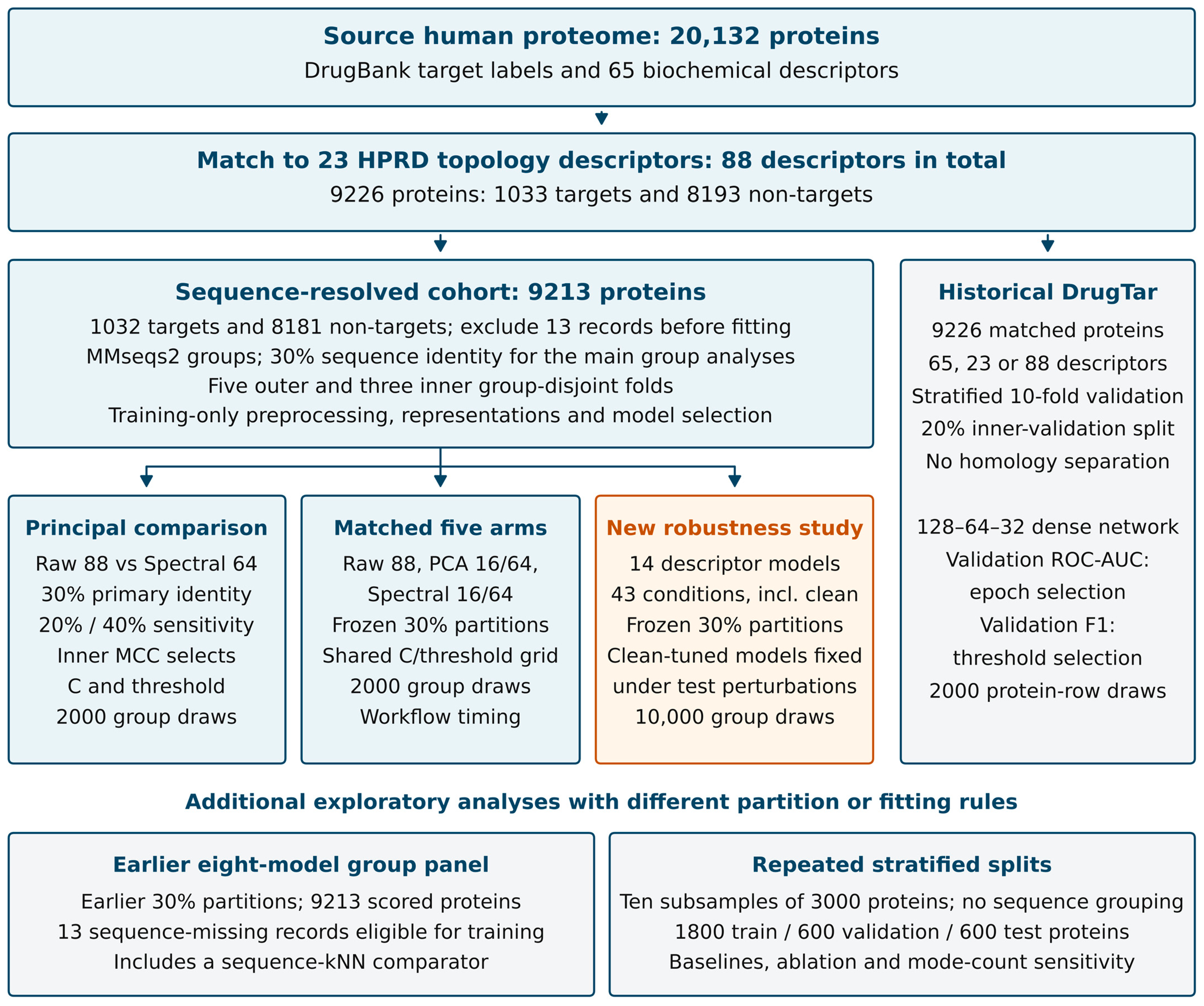
The historical intervals and tests condition on the fitted models, partitions, and predictions; they exclude variation from renewed clustering, splitting, fitting, or model selection. These analyses were exploratory, and margin-specific p-values were nominal rather than multiplicity-adjusted confirmatory evidence. Statistical learning used scikit-learn [48]; software versions and random seeds for each analysis are provided in Appendix A. Figure 1 summarizes the study design.
Figure 1.
Dataset lineage and evaluation protocols. The source dataset [8] forms a 9226-protein descriptor cohort after accession matching. The sequence-resolved cohort excludes 13 records before fitting. The principal analysis, historical five-arm benchmark and new 14-model robustness experiment use the specified homology-disjoint protocols but remain separate realized fits. The historical 9226-protein DrugTar feature-set experiment and the older exploratory panels use different protocols (Table 3). The new robustness arm for DrugTar uses the common frozen CSVs and homology folds. HPRD: Human Protein Reference Database; MCC: Matthews correlation coefficient.
2.10. Computational Complexity and Matched Runtime/Memory Benchmark
We assessed computational scaling in two complementary ways. First, we derived analytical operation and storage orders from the procedures in Section 2.3 and Section 2.4. Second, we measured complete-method wall time and peak process memory for Raw-88, PCA-16, PCA-64, Spectral-16, and Spectral-64 under the same homology-disjoint 30% identity partitions, cohort eligibility, and tuning rules as the principal analysis (Section 3.5; principal_matched/ in the consolidated supplementary archive). Let n denote the number of training proteins, p = 88 the descriptor dimension, k = 15 the neighbor count, r the retained graph modes (64 in the principal model), T = 5 the number of residual updates, and q the number of held-out proteins. Exhaustive cosine-similarity graph construction requires O(n2p) arithmetic; the sparse symmetrized k-nearest-neighbor adjacency has at most O(nk) nonzero entries. A truncated symmetric eigensolver uses iterative sparse matrix–vector products and orthogonalization, with data-dependent convergence; its realized iteration count is unavailable [33].
Given an n × r eigenvector matrix, applying the factorized rank-r operator to an n × p signal requires O(nrp) arithmetic per filtering step, or O(Tnrp) across T steps. Eigenvector storage is O(nr), sparse graph storage is O(nk), and the rolling training state and filtered signal require O(np) storage. The supplied implementation advances training and query states together and does not persist a T-step history. Query states and the sparse cross-neighbor map add O(qp + qk) storage. Exhaustive neighbor search may also require O(n2) temporary similarity storage, depending on numerical-library chunking. In the measured benchmark, memory was the absolute process peak resident/working-set size through predictions (Windows PeakWorkingSetSize), including interpreter, imports, and data loading. The transformed state retains 88 columns, so the downstream SVM has 88 coefficients and an intercept, as in Raw-88.
For q inductive queries, brute-force matching to n training proteins requires O(qnp) cosine-comparison work. Given each filtered training signal, the additional query updates require O(qTkp), followed by O(qp) SVM scoring. The supplied implementation computes those training signals within the same transformation call; a deployment implementation could instead cache them at O(Tnp) storage, but such persistent caching was not included in the historical resource benchmark. The new robustness implementation uses a parity-validated cache to apply many test corruptions; its execution times are not substituted for the historical benchmark. Replacing r = 64 with r = 16 reduces eigenvector entries and rank-dependent projection arithmetic by 75% without reducing p, k, T, or the exact neighbor-search work. Measured workflow time covers all three inner preprocessing/representation fits and transforms, the four-value C grid, pooled-inner threshold selection, and the final outer fit and held-out prediction. It excludes process startup, shared input loading, split validation, original descriptor generation, MMseqs2 search, and metric/bootstrap reporting. The measurements are combined nested workflows, not separate training-only or inference-only end-to-end benchmarks.
For the reviewer-requested matched spectral-resolution analysis, the retained graph mode count was set separately to 16 or 64; both representations preserved all 88 output columns. Raw-88 and PCA with 16 or 64 output components were fitted as reference arms. Matched-run PCA used full singular value decomposition without whitening; the earlier exploratory panel used randomized decomposition (Table A3). The five arms used the same 9213-protein eligibility rule, frozen outer and inner 30% identity partitions, fold-local median imputation and scaling, class-weighted linear SVM, C candidates {0.1, 0.3, 1, 3}, and a pooled-inner operating-threshold search over 301 score quantiles plus zero. Each method and outer fold was fitted independently; the lower-rank spectral arm was not charged for constructing the 64-mode eigensystem. MCC and average precision (AP) were calculated from held-out pooled out-of-fold predictions. Matched method contrasts used identical multiplicity weights in 2000 homology-group bootstrap resamples, yielding unadjusted percentile 95% intervals conditional on these fitted predictions; intervals do not include refitting or the earlier development-stage selection. Frozen split identifiers, model settings, out-of-fold scores, and analysis/benchmark scripts are supplied under principal_matched/ in the consolidated supplementary archive. The earlier principal-run scores and new matched-run scores are not mixed or treated as bit-identical.
The historical separately adapted DrugTar descriptor network provides a parameter-count reference, not a matched computational benchmark. Its 88–128–64–32–1 dense architecture, including affine biases and the trainable scale and offset of each batch-normalization layer, has 22,209 trainable parameters: (88 × 128 + 128) + (128 × 64 + 64) + (64 × 32 + 32) + (32 + 1) + 2(128 + 64 + 32). This is about 250 times the 89 SVM classification coefficients. In that historical comparison, DrugTar training used different partitions and operating policies, and graph eigenvectors, current states, and neighbor-search intermediates also consume resources; parameter counts do not demonstrate comparative speed or accuracy.
2.11. Comparative Robustness Assessment
We conducted an additional, separately fitted robustness experiment informed by the assessment framework in ISO/IEC TR 24029-1:2021 [49], the formal-methods scope of ISO/IEC 24029-2:2023 [50], and the statistical-methods draft ISO/IEC DIS 24029-3 [51]. The assessment objective was maintenance of predictive performance under specified technical input corruptions. The protocol fixed the candidate, comparators, perturbations, endpoints, and comparison families before new robustness outcomes were examined. It was an exploratory evaluation of a previously studied cohort, not an externally registered confirmatory study, an ISO conformity assessment, or a deployment pass/fail test. No application-validated acceptable-degradation threshold was available.
Fourteen descriptor-based models used the exact frozen CSV inputs for the 9213 sequence-resolved proteins and the original five outer and three inner 30% identity partitions. Spectral-64 was the primary candidate, and Raw-88 and PCA-64 were primary controls. Spectral-16, PCA-16, truncated-SVD-64, uniform-spectral-64, heat-diffusion-64, label propagation, L1 logistic regression, RBF-SVM, Extra Trees, histogram gradient boosting, and the DrugTar descriptor architecture completed the panel (Table A27). All preprocessing and representation fitting used clean training records only. Inner predictions selected parameters and the operating threshold; complete outer-training refits were frozen before corrupting test inputs. The DrugTar architecture and optimizer were recovered, whereas other reconstructed controls are explicitly identified. Sequence-kNN was excluded from descriptor-corruption contrasts because its sequence input would remain unchanged.
Every model received identical corrupted raw test matrices. Primary families comprised independent missing entries at probabilities 0.01, 0.05 and 0.10, and additive Gaussian noise with standard deviation 0.01, 0.05 and 0.10 times each continuous feature’s clean-training standard deviation. Each severity had three fixed random draws. Feature types were inferred from outer-training values: 69 binary, four integer-valued and 15 noninteger continuous columns in every fold. Noise and rounding acted only on the 15 continuous columns. Negative noisy values were clipped to zero when that training column was entirely nonnegative; this empirical-support restriction does not establish a biological constraint. Missing entries were handled by the unchanged training-median imputer. Secondary scenarios comprised 20% missingness/noise, binary-one deletion, significant-digit rounding and separate topology/biochemical block removal (Table A26). Together with clean inputs, these formed 43 scenarios. Shared random directions or masks paired severities; seeds did not depend on model identity or labels.
For each scenario, pooled out-of-fold MCC was calculated before averaging equally over severities and random draws. Performance loss was clean MCC minus mean corrupted MCC; the paired loss advantage was comparator loss minus spectral loss, so positive values favored spectral retention. Absolute corrupted MCC, AP, ROC-AUC, sensitivity, specificity, and harmful/corrective prediction changes were also retained. The four primary contrasts compared Spectral-64 with Raw-88 and PCA-64 in the two primary families. Whole homology groups were resampled with identical multiplicities across models, clean/corrupted scenarios and repetitions. The final analysis used 10,000 draws, two-sided centered-bootstrap tests with a plus-one Monte Carlo correction, and pointwise 95% percentile intervals. Holm adjustment [52] was applied separately to four primary MCC contrasts, 120 secondary MCC contrasts, and four exploratory AP contrasts on the primary scenario grid. A retention advantage required a positive estimate and adjusted p < 0.05; uncertainty remained conditional on fitted models and fixed corruption draws.
An implementation review identified that 2000 planned draws could not yield a first Holm-adjusted p below 0.05 across 120 secondary tests, because 120/2001 = 0.05997. Before comparative effects were inspected, a documented precision amendment increased all inference to 10,000 draws without changing hypotheses, models, thresholds or corruption seeds. The protocol, amendment and all results are supplied. The new DrugTar arm retained the historical architecture and optimizer but used the common frozen CSVs and homology folds: inner ROC-AUC early stopping selected epochs, the median inner-selected epoch count determined a full outer-training refit, and pooled-inner MCC selected the threshold. This differs from the historical non-grouped, inner-F1, no-refit experiment in Section 2.8.
A separate analytical assessment considered local decision stability in continuous standardized-input L2 balls with fitted training states and thresholds fixed. Exact affine boundary distances for Raw/PCA/SVD were compared descriptively with conservative nonlinear spectral lower bounds accounting for neighbor membership, changing query weights and all normalization updates (Appendix A.8). Differently tight bounds were not treated as unbiased estimates of actual adversarial robustness. Neither sampled stress tests nor these numerically evaluated exact-real-arithmetic bounds establish end-to-end floating-point verification or formal robustness superiority.
3. Results
3.1. Sequence-Group Evaluation
At 30% sequence identity, the 9213 proteins formed 6462 groups, including 5186 singletons, 1276 multi-protein groups, and 181 mixed-label groups; the largest group contained 90 proteins. There were 7008 qualifying undirected edges. The 20% and 40% conditions produced 6164 groups (9299 edges; largest group 145) and 7010 groups (4153 edges; largest group 48), respectively. All audited inner and outer splits had zero shared groups and zero qualifying cross-split edges.
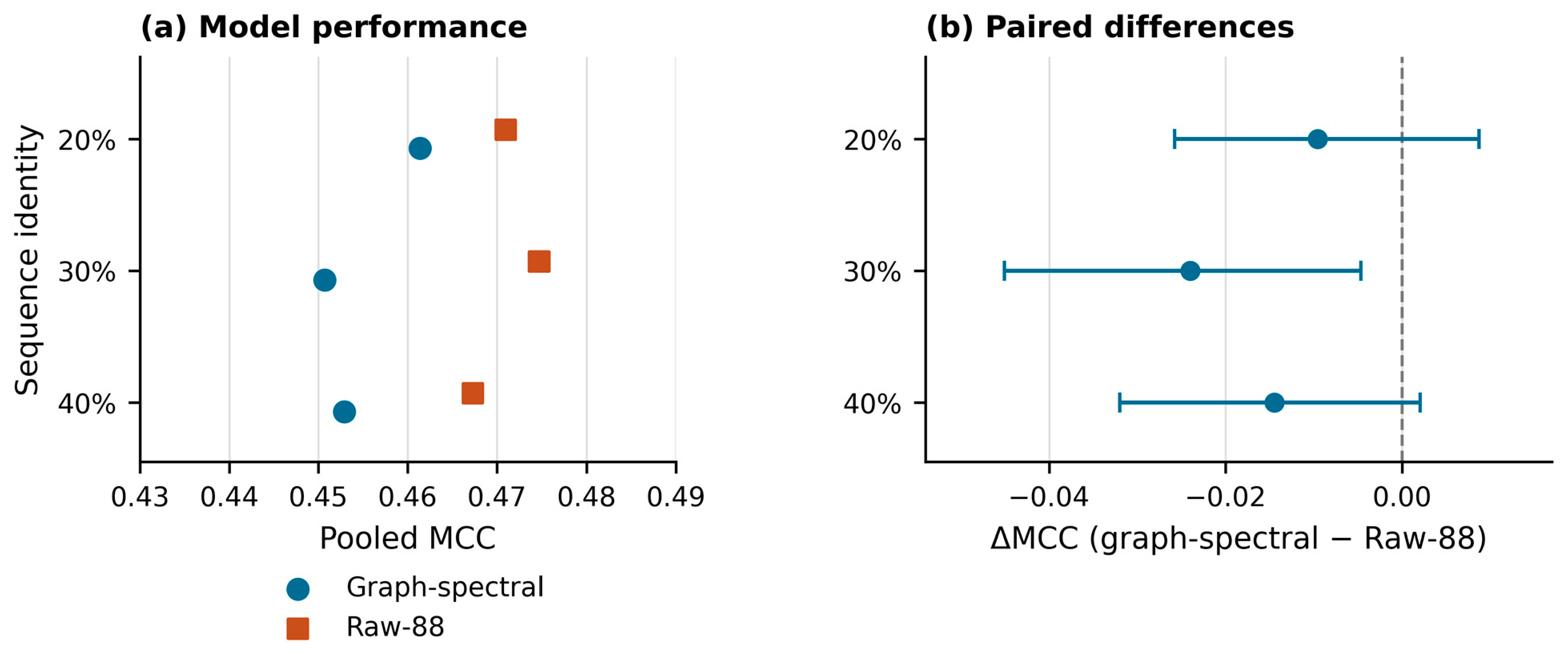
At 30% sequence identity, graph-spectral MCC was 0.4507, and Raw-88 MCC was 0.4747; ROC-AUC was 0.8613 and 0.8654, and average precision (AP) was 0.4812 and 0.4874, respectively (Table 4). The observed paired MCC difference was −0.0240, with a conditional group-bootstrap 95% interval of −0.0451 to −0.0047 (Table 5; Figure 2). The normal-approximation difference test gave p = 0.0182. At 20% and 40% identity, the MCC differences were −0.0095 and −0.0144, respectively, with both 95% intervals spanning zero.
Table 4.
Pooled out-of-fold performance in the principal 9213-protein analysis. MCC: Matthews correlation coefficient; ROC-AUC: area under the receiver operating characteristic curve; AP: average precision.
Table 5.
Paired graph: spectral minus Raw-88 MCC differences in the principal analysis. Intervals are conditional 95% group-bootstrap intervals from 2000 replicates.
Figure 2.
Principal sequence-group comparison across identity thresholds. (a) Pooled out-of-fold Matthews correlation coefficient (MCC) for the graph-spectral model and Raw-88. (b) Observed paired MCC differences, with conditional 95% intervals from 2000 sequence-group bootstrap replicates. The dashed line denotes equal MCC. Differences are defined as graph-spectral minus Raw-88; 30% identity is the principal condition. Estimates are reported in Table 4 and Table 5.
In the equivalence sensitivity analysis, the paired group-bootstrap standard error was 0.01017, and the normal-approximation 90% interval was −0.0407 to −0.0073. The ±0.05 MCC criterion was met (pTOST = 0.0053), whereas ±0.04 was not (pTOST = 0.0578); the narrower ±0.01, ±0.02, and ±0.03 criteria were also not met (Table A23). These are post hoc, margin-specific findings conditional on the fitted predictions, not evidence of exact equality or practical interchangeability under a prespecified bound.
At 30% identity, graph-spectral predictions comprised 659 true positives, 373 false negatives, 7309 true negatives, and 872 false positives. Raw-88 yielded 682, 350, 7344, and 837, respectively. Across folds, mean MCC was 0.4489 ± 0.0725 for the graph-spectral model and 0.4731 ± 0.0566 for Raw-88. The graph-spectral model had higher MCC in one of five folds. Fold-level estimates are presented in Table A4 and Table A5.
3.2. Exploratory Sequence-Group Comparator Panel
The exploratory sequence-group panel characterized performance across alternative representations on common partitions (Table 6). Pooled MCC was 0.4590 for the graph-spectral model, 0.4725 for Raw-88, 0.4804 for PCA, and 0.4795 for truncated SVD. The uniform spectral filter yielded MCC 0.4636. These point estimates describe this panel and its specific eligibility and threshold-selection rules.
Table 6.
Pooled out-of-fold performance in the exploratory 30% sequence-group comparator panel (9213 scored proteins). The panel used the eligibility and threshold-search protocol specified in Table 3. Note: Table 6 and Table A12 use the same scored outer test-protein sets but differ in training eligibility and neighbor-search configuration. Table 6 retains sequence-missing proteins as eligible training records and uses n_jobs = 2; Table A12 excludes them before fitting (complete-case also removes O00526) and uses n_jobs = 1. Both use the 301-quantile-plus-zero threshold rule. Exact equality of the historical inner partitions cannot currently be independently verified because the archived inner-assignment file is empty. These protocol differences preclude interpreting the between-table contrast as an isolated imputation effect for either Raw-88 or the graph-spectral model; their individual contributions have not been isolated.
Bootstrap mean MCC differences for the graph-spectral model relative to PCA and truncated SVD were −0.0215 (95% interval −0.0374 to −0.0054) and −0.0206 (−0.0365 to −0.0046), respectively. The interval relative to the uniform spectral filter included zero. The graph-spectral differences relative to graph heat diffusion, label propagation, and sequence-kNN were positive in this panel. Pairwise intervals and fold-level results are provided in Table A6 and Table A7. These exploratory contrasts characterize representation effects within the panel; they do not establish a general ranking of published methods.
3.3. Sensitivity Analyses
3.3.1. Baseline Models and Missing-Data Sensitivity
Across ten repeated stratified splits, the graph-spectral model achieved mean MCC 0.4539, compared with 0.4230 for L1 logistic regression and 0.4062 for the raw-feature linear SVM (Figure 3; Table A10). Extra Trees, classical graph diffusion, histogram-based gradient boosting, and the tuned radial-basis-function SVM yielded mean MCCs of 0.4210, 0.4172, 0.3948, and 0.3868, respectively (Table A14). AP was 0.4698 for logistic regression and 0.4636 for the graph-spectral model. Relative performance was therefore metric-dependent under a protocol that allowed sequence-related proteins to appear in different partitions.
Figure 3.
Baseline performance across ten repeated stratified splits of the matched protein cohort. Bars show mean test Matthews correlation coefficient (MCC); error bars show one standard deviation. The splits overlap and do not enforce sequence-group separation. SVM: support vector machine; RBF: radial basis function. Numerical estimates are provided in Table A14.
Replacing zero-fill with training-median imputation had little effect on repeated-split performance. In a separate sensitivity analysis using the earlier 30% sequence-group partitions, graph-spectral MCC was 0.4447 with median imputation, 0.4560 with zero-fill, and 0.4605 after complete-case exclusion, whereas Raw-88 remained between 0.4745 and 0.4750 (Table A11 and Table A12). Within that sensitivity panel, the graph-spectral results varied more than the raw-feature results. These changes do not isolate an effect relative to Table 6, which also differs in training eligibility and historical implementation records.
3.3.2. Ablation of Graph-Spectral Components
The full graph-spectral model yielded mean MCC 0.4539. Removing exponential mode weighting, retaining only the nonlinear state, limiting propagation to one step, and using plain graph propagation yielded 0.4420, 0.4383, 0.4371, and 0.4249, respectively (Figure 4; Table A15). All four paired seed-level 95% intervals included zero, and the AP ordering differed from the MCC ordering. The ablations therefore describe sensitivity to component choice without isolating a necessary contribution from any single component.
Figure 4.
Ablation of graph-spectral components under repeated stratified splits. Bars show mean test Matthews correlation coefficient (MCC); error bars show one standard deviation across ten overlapping splits. The rank-64 uniform filter retains 88 output features. Paired full-model-minus-ablation differences and intervals are provided in Table A15.
3.3.3. Spectral Resolution and Descriptor Contributions
In the descriptive mode grid, 64 modes yielded the highest mean MCC (0.4539), whereas 16 modes yielded the highest AP (0.4742; Figure 5a; Table A16). The 16-mode representation had mean MCC 0.4508 and AP 0.4742, compared with MCC 0.4539 and AP 0.4636 for 64 modes. Thus, fourfold higher mode count changed mean MCC by only approximately 0.003, while AP favored the smaller mode budget by 0.0106. The first 64 modes captured 84.66% of feature spectral energy and 88.32% of training-label spectral energy relative to the first 128 computed modes (Figure 5b). Increasing retained energy did not yield monotonic improvement in discrimination or MCC. Selection of the mode count on validation data gave a mean MCC of 0.4358 and chose 16 modes in four of ten splits (Table A18). These analyses use overlapping, non-homology-disjoint splits; the observed mode trade-off is exploratory and cannot establish inferential equivalence, optimal rank, or faster measured execution.
Figure 5.
Sensitivity to spectral resolution under ten repeated stratified splits. (a) Mean test Matthews correlation coefficient (MCC), with one-standard-deviation error bars. (b) Mean cumulative feature and training-label spectral energy, normalized to the first 128 computed modes. These descriptive mode-grid results do not represent independent test sets; mode selection using validation data is reported in Table A18.
Further PCA/SVD comparisons, supervised descriptor profiles, and descriptor-subset ablations are presented in Table A19, Table A20 and Table A21. Removing selected biochemical or topology descriptors reduced the graph-minus-raw MCC difference, but these subsets were chosen post hoc. These analyses support a distributed, protocol-dependent contribution of the descriptors rather than a unique graph-spectral or biological mechanism.
3.4. Performance of the DrugTar Classifier
Within the historical separate stratified 10-fold experiment, combined descriptors yielded ROC-AUC 0.8705, AP 0.4952, and MCC 0.4740 at the inner-F1 operating point. Biochemical features yielded 0.8551, 0.4675, and 0.4504, whereas topology features yielded 0.6371, 0.2023, and 0.1370 (Table 7). The observed combined-minus-biochemical MCC difference was +0.023567, with a conditional paired protein-row bootstrap 95% interval of +0.006373 to +0.041723. This is a matched feature-set comparison within the descriptor adaptation.
Table 7.
DrugTar-classifier descriptor adaptation at the inner-F1 operating point. Parentheses contain conditional protein-row bootstrap 95% intervals.
The combined model produced 701 true positives, 332 false negatives, 7295 true negatives, and 898 false positives, corresponding to sensitivity 67.86%, specificity 89.04%, and precision 43.84%. Its MCC was 0.4731 with inner-MCC threshold selection and 0.4071 at a fixed probability threshold of 0.5 (Table A22). These results demonstrate sensitivity to the operating policy within the descriptor experiment. This historical experiment evaluates descriptor combinations within the DrugTar architecture. Its cohort eligibility, partitions, and model-selection procedure differ from the graph-spectral experiment, so those historical results are not a head-to-head comparison of the two methods. The new matched DrugTar robustness arm is reported separately in Section 3.7.
3.5. Computational Interpretation and Mode-Budget Trade-Off
Table 8 separates the additional operations of the graph-spectral arm from those of Raw-88 on an analytical basis. Both models use a class-weighted linear SVM with 89 classification coefficients, contrasting architecturally with the 22,209 trainable parameters calculated for the separately adapted DrugTar descriptor network. That historical architectural and resource comparison does not constitute a matched predictive comparison with the network; the new descriptor-only DrugTar robustness comparison is reported in Section 3.7. The graph filter introduces exhaustive graph-neighbor comparisons, a truncated eigensystem, and five spectral propagation updates; these extra stages are not compensated by a reduction in descriptor columns. Table 9 reports the matched empirical complete-method wall time and peak process memory under the principal homology-disjoint protocol (one measurement per method–fold; mean ± SD across five outer folds). Spectral-64 required 57.25 ± 1.32 s wall time and 1015.8 ± 22.4 MiB peak working set, versus 32.79 ± 2.95 s and 182.3 ± 0.5 MiB for Raw-88 and 32.11 ± 7.59 s and 185.5 ± 0.3 MiB for PCA-64. Spectral-16 was only modestly faster (52.70 ± 1.29 s) with essentially the same peak memory (1015.0 ± 22.7 MiB). Applied settings recorded in the run manifest were Windows 10, Intel Core i5-3210M @ 2.50 GHz, 4 logical CPUs, Python 3.12.3 with the package versions listed in the matched package, and numerical thread limits fixed at 2 (OpenBLAS/OpenMP num_threads = 2 in per-job threadpool records). Physical core count and installed system RAM were not stored in the run manifest. These measurements do not support a computational advantage for the graph-spectral method over the matched simpler controls.
Table 8.
Analytical computational requirements of the graph-spectral and matched Raw-88 arms. Here n is the training-set size, q the number of queries, p = 88, k = 15, r the retained eigenmodes, and T = 5. Costs are theoretical operation counts or storage orders. Measured wall times and peak memory appear in Table 9.
Table 9.
Matched complete-method wall time and peak process memory (mean ± SD across five outer folds; one measurement per method–fold). Timing covers nested inner fits, C/threshold selection, and outer fit/prediction under the disclosed scope; memory is peak process working set.
Among the seven mode counts studied on repeated stratified splits (Table A16), only 16 and 64 modes were non-dominated on the pair of reported mean metrics, MCC and AP (Figure 6). The fourfold mode-count difference corresponded to an MCC difference of approximately 0.003 in favor of 64 and an AP difference of 0.0106 in favor of 16. The 16-mode basis has 25% as many stored eigenvector entries and 25% of the leading rank-dependent projection operations at fixed n, p, and T. This is a descriptive, post-development resolution trade-off: the splits are overlapping, do not separate homologous proteins, and cannot establish practical equivalence, a validated Pareto frontier, or an end-to-end efficiency gain. A separate matched homology-disjoint comparison of 16- versus 64-mode spectral models (with Raw-88 and PCA references) is reported in Section 3.6 and Table 10 and Table 11 and does not establish a confirmatory 64-mode optimum under the principal partitions.
Figure 6.
Exploratory performance trade-off over seven retained eigenmode counts. The points reproduce mean test MCC and AP from Table A16 (ten overlapping, non-homology-disjoint stratified splits); marker area is proportional to the mode count. The dashed segment links the two descriptively non-dominated settings (16 and 64 modes). This is a post hoc graphical synthesis, not a cost measurement or an inferentially validated Pareto frontier.
Table 10.
Pooled held-out performance in the matched 30% identity analysis (9213 proteins; five homology-group-disjoint outer folds). The graph-spectral arms both output 88 descriptors; PCA-16/64 output 16/64 principal components. All estimates come from the same saved matched-run out-of-fold records, not the earlier principal or exploratory comparator panels.
Table 11.
Paired differences (A minus B) in the matched mode comparison. Conditional 95% percentile confidence intervals are from 2000 paired resamples of homology-connected components with the same group weights applied to each model. Differences use unrounded pooled estimates, so subtraction of displayed Table 10 values may differ in the last decimal. The Spectral-16 versus PCA-64 contrast was additionally derived from the saved paired replicates during the final revision. These exploratory intervals are not adjusted for multiple comparisons or model selection.
3.6. Matched 16-Versus-64-Mode Comparison on Homology-Disjoint Folds
The additional comparison requested during peer review was conducted as a separate, matched re-fit on the principal 9213 sequence-resolved proteins and the same five 30% identity outer/inner partition assignments (6462 homology groups). All five arms underwent independent train-only representation fitting and identical C/threshold selection rules. Table 10 reports pooled out-of-fold classification performance. The 16-mode spectral arm achieved MCC 0.4767, ROC-AUC 0.8711, and AP 0.4726; the 64-mode arm achieved MCC 0.4579, ROC-AUC 0.8633, and AP 0.4745. The matched Raw-88 and PCA-64 controls achieved MCC 0.4740 and 0.4771, respectively. These values describe the matched re-fit and are not replacements for the historically frozen principal estimates in Table 4.
Using 2000 paired homology-group bootstrap replicates, Spectral-64 minus Spectral-16 MCC was −0.0188 (conditional 95% interval −0.0366 to −0.0020), whereas its AP difference was +0.0018 (−0.0217 to +0.0243). The nominal MCC contrast favored the smaller spectral representation; the AP interval included zero. Spectral-16 minus Raw-88 MCC was +0.0027 (−0.0107 to +0.0163), so no superiority to the raw-feature control is demonstrated. An additional exploratory comparison with the strongest matched linear representation, PCA-64, gave a Spectral-16 minus PCA-64 MCC difference of −0.0004 (−0.0158 to +0.0157) and AP difference of −0.0190 (−0.0362 to −0.0007). The latter nominal interval favored PCA-64. These contrasts were calculated from the same saved paired bootstrap replicates; Table 11 reports the selected comparisons. CIs are unadjusted, conditional on fixed out-of-fold models and a cohort whose representation choices were explored during development; they are not independent validation or evidence of a prespecified equivalence margin.
The new matched re-fit was not numerically identical to the archived principal run: the matched Spectral-64 MCC was 0.4579 versus principal MCC 0.4507, with 178 of 9213 classifications differing (1.93%); the Raw-88 predictions differed for one protein. Fold-specific Spectral-64 operating thresholds and, in some folds, C values also changed. The frozen input/split records match, but historical numerical-platform, eigensolver, and neighbor-tie details have not been fully reconstructed; a fixed-thread explanation alone is insufficient. For transparency, Table 4 and Table 5 retain the original principal-run values and Table 10 and Table 11 report the later matched re-fit without selecting the more favorable estimate post hoc.
3.7. Comparative Robustness Under Held-Out Descriptor Corruption
The new robustness evaluation generated 5,546,226 held-out scores across 14 models, 43 scenarios and 9213 proteins. All 215 fold/scenario input matrices passed independent corruption-policy checks. Every saved score was replayed from fitted states; maximum absolute discrepancy was 4.44 × 10⁻¹⁶. Clean MCC in this new fit was 0.4597 for Spectral-64, 0.4760 for Spectral-16, 0.4747 for Raw-88, 0.4777 for PCA-64 and 0.4840 for the matched DrugTar descriptor arm (Table 12). These are new within-experiment baselines; they do not replace principal Table 4 or historical matched Table 10 values.
Table 12.
Clean and mean corrupted MCC in the new homology-matched robustness experiment. Each primary family averages three severity levels (1%, 5%, 10%) and three random draws per level. Loss is clean minus corrupted MCC; negative loss denotes a small improvement under that perturbation. All 14 models use the same held-out inputs.
Under primary random missingness, Spectral-64 lost 0.0100 MCC compared with 0.0269 for Raw-88. The paired retention advantage was +0.0169 (conditional 95% interval +0.0090 to +0.0245; Holm-adjusted p = 0.0004), a descriptive 62.8% reduction in mean loss. Mean corrupted MCC was 0.4497 versus 0.4478; its absolute difference of +0.0019 (−0.0169 to +0.0185) did not establish superior absolute performance. Missingness versus PCA-64 and both continuous-noise primary contrasts were not significant after adjustment (all p = 0.5492; Table 13; Figure 7 and Figure 8).
Table 13.
Four planned primary MCC contrasts for Spectral-64. Positive loss advantage favors spectral retention; positive absolute difference favors spectral corrupted performance. Intervals are pointwise conditional 95% group-bootstrap intervals; p-values use Holm correction over the four retention contrasts. Absolute-performance intervals are descriptive and not multiplicity-adjusted.
Figure 7.
Severity-dependent performance of the primary candidate, secondary spectral rank and primary controls in the new robustness experiment. Panels: (a) MCC under random entry missingness; (b) MCC under clipped Gaussian continuous-feature noise; (c) AP under random entry missingness; (d) AP under clipped Gaussian continuous-feature noise. Points average three fixed draws per nonzero severity; clean performance is plotted at zero. Levels 1%, 5% and 10% enter primary averages; 20% is secondary. Noise SD is relative to each feature’s training SD and affects only 15 continuous features. Solid/dashed curves join severity point estimates; solid lines cover primary severities (0–10%) and dashed lines reach the secondary 20% point. Curves are point estimates, not confidence bands. Curves are point estimates, not confidence bands.
Figure 8.
Performance-retention contrasts for Spectral-64 on the primary corruption grid. (a) Four planned MCC contrasts. (b) Four exploratory AP contrasts. Positive effects indicate a smaller clean-to-corrupted performance loss for Spectral-64. Bars are pointwise conditional 95% intervals from 10,000 paired whole-group bootstrap draws. Displayed p-values are Holm-adjusted separately within the four MCC and four AP tests. Retention advantages do not by themselves establish higher absolute corrupted performance (Table 13 and Table A28).
AP corroborated missingness retention versus Raw-88: losses were 0.0088 and 0.0317, with an advantage of +0.0229 (95% interval +0.0150 to +0.0302; exploratory Holm-adjusted p = 0.0004). Absolute corrupted AP remained numerically lower for Spectral-64 (0.4448 versus 0.4557; difference −0.0110, interval −0.0320 to +0.0088). No AP retention advantage was established over PCA-64 or under continuous noise (Table A28). PCA-64 retained higher absolute AP under both primary families. Noise had small effects on MCC for most arms; synthetic perturbations occasionally increased the selected-threshold metric.
Ten positive and one negative retention contrasts survived Holm correction across 120 secondary comparisons. Both spectral ranks had smaller rounding-related MCC loss than Raw-88, PCA-64, SVD-64 and RBF-SVM, and smaller full-grid missingness loss than Raw-88. Rounding advantages were largely driven by the two-significant-digit condition: MCC was 0.4292 for Spectral-64, 0.3523 for Raw-88 and 0.2890 for PCA-64. At three significant digits, Spectral-64 remained below Raw-88 and PCA-64 (Table A29; Figure A1). Spectral-16 had greater loss than Heat-64 under averaged whole-block removal (adjusted p = 0.0440). No general advantage was established under continuous noise, annotation deletion or block removal, or over uniform spectral, diffusion, label-propagation, tree/boosting, logistic or DrugTar controls (Figure A2; full contrasts supplied).
The analytical local-bound calculation did not establish a formal spectral advantage (Table A30). At standardized L2 radius 0.01, the correct-and-stable lower-bound fractions were 24.62% for Spectral-64 and 24.80% for Spectral-16, compared with 87.02% and 86.53% from the exact affine boundaries of Raw-88 and PCA-64. The spectral bounds restrict the neighbor set and are conservative; smaller bounds cannot establish worse actual adversarial robustness. Thirty-seven queries per spectral arm had inconclusive zero bounds at neighbor-membership ties. These results concern exact-real mathematical maps evaluated numerically, not validated floating-point software or biological guarantees.
The new Linux execution is not assumed identical to archived Windows fits. As a direct check, unmodified original code for PCA-64 and Spectral-64 on outer fold 1 reproduced the new cached runner’s clean scores, selected C and thresholds exactly, while both differed from archived historical scores. This rules out caching as the cause for those checked discrepancies but does not isolate every historical numerical factor. The three realized evaluations—principal, historical five-arm benchmark and new robustness refit—remain separately reported.
4. Discussion
4.1. Principal Findings
Under the principal 30% sequence-group protocol, the graph-spectral representation achieved ROC-AUC 0.8613 and MCC 0.4507, compared with 0.8654 and 0.4747 for the matched Raw-88 model. The observed paired MCC difference of −0.0240 (conditional 95% interval, −0.0451 to −0.0047) favored Raw-88. The exploratory sequence-group panel also favored PCA and truncated SVD in MCC, precluding any claim of general predictive superiority for the graph operator. A post hoc equivalence analysis met the illustrative ±0.05 MCC criterion (p = 0.0053) but not ±0.04 (p = 0.0578); neither bound was prespecified or justified as negligible. These sensitivity results should not be construed as confirmatory non-inferiority or interchangeability.
Across repeated stratified splits, mean graph-spectral MCC differences were +0.0309 relative to logistic regression and +0.0478 relative to the raw-feature linear SVM, while AP was 0.4636 for the graph-spectral model, 0.4698 for logistic regression, and 0.4554 for the raw-feature linear SVM. This variation across metrics and protocols emphasizes the role of the representation and operating policy in the measured endpoint. Training sizes, partitions, tuning budgets, and threshold policies differed from the sequence-group analyses, so the change in relative performance cannot be attributed solely to homology separation.
4.2. Interpretation of the Representation
The representation combines truncated graph projection, normalized positive exponential eigenmode weights, elementwise nonlinearity, five fixed residual propagation steps, and row normalization [22,23]. The Hamiltonian analogy is limited to the symmetry and spectral decomposition of the graph operator. It is neither unitary quantum evolution nor a physically specified Hamiltonian of protein interactions and supplies no basis for claiming quantum computational advantage. The five residual updates are a fixed representation depth, not an observed number of optimizer iterations or a convergence advantage.
The uniform-weight ablation, graph diffusion, and PCA/SVD comparators distinguish spectral weighting from ordinary low-rank representation and nonlinear propagation. However, no ablation established a statistically necessary contribution for an individual component. The 64 retained eigenmodes belong to the training-protein graph, whereas the final state still contains 88 descriptor columns and the linear SVM has 88 slope coefficients and an intercept. Spectral-energy concentration was not predictive of MCC across mode counts, so retaining more modes should not be conflated with stronger protein classification. The exploratory 16-mode result alone did not establish an operational benefit; in the separate measured matched analysis, 16 modes modestly reduced wall time relative to 64 modes, but both spectral variants remained slower and more memory-intensive than Raw-88 and PCA (Table 9, Table 10 and Table 11).
The historical missing-data sensitivity panel showed variation when treatment of five values in one incomplete protein changed. Because training eligibility and historical inner-partition records differed across panels, that comparison cannot isolate an imputation mechanism. The new controlled experiment instead perturbs held-out descriptors after fixing fitted preprocessing, representations and thresholds. It supports smaller missingness-induced MCC and AP loss than Raw-88, without establishing higher absolute corrupted performance or a retention advantage over PCA-64. It therefore answers a different, explicitly defined robustness question rather than retrospectively resolving the historical training-imputation discrepancy.
4.3. Specific Contribution and Computational Interpretation
The concrete algorithmic contribution is a fully specified, train-only descriptor-similarity filter combining a symmetric graph operator, rank-truncated eigenmode weighting, nonlinear residual states, and an inductive neighbor-based map for unseen proteins. Because the graph basis and filtered training signals depend on training data, the absence of additional supervised feature-map coefficients should not be equated with a parameter-free or inexpensive computational pipeline. Nor does a graph eigenvector automatically provide a biologically causal explanation. The distinctive experimental contribution lies in testing this representation against a matched raw classifier and simple dimensionality-reduction and diffusion alternatives under explicit sequence-homology constraints. The new robustness experiment adds a specific empirical contribution: improved retention relative to Raw-88 under random missing descriptors and exploratory tolerance to coarse numerical quantization. These findings concern the full fitted pipeline; they do not identify the exponential Hamiltonian-inspired weights as the necessary cause.
The results also delineate the limitation of the proposed inductive bias. Raw-88 was better in the principal paired test, PCA/SVD were stronger in the exploratory sequence-group panel, and the nonlinear and weighting ablations did not isolate an indispensable component. At the same time, 16 versus 64 modes provided an exploratory AP–MCC trade-off with a fourfold difference in rank-dependent storage and projection work. The matched homology-disjoint analysis further found lower MCC for Spectral-64 than Spectral-16 (Δ = −0.0188; conditional 95% interval −0.0366 to −0.0020), without an AP advantage that excludes zero; Spectral-16 also did not clearly outperform Raw-88 (Table 11). Together, these observations offer a falsifiable account of when graph spectral resolution may be unnecessary, rather than evidence of state-of-the-art accuracy or quantum acceleration. The negative principal finding remains methodologically informative. The additional retention result describes a conditional trade-off despite lower clean performance, rather than overturning that finding or establishing general superiority.
4.4. Dataset Meaning and Relation to Previous Work
The source paper defines the labels as approved-drug target annotations [8]; the present study is therefore a reanalysis of that annotation task. The labels do not directly measure disease-specific therapeutic relevance or intrinsic druggability. The negative class may include proteins that were uncharacterized at the historical snapshot or became targets later. The HPRD intersection also selects proteins with recorded interactions and raises target prevalence relative to the source proteome. Performance therefore applies to this historically annotated, network-covered population and cannot be generalized to all human proteins without further assessment.
The distinction between upstream and downstream graphs is essential. HPRD topology is part of the fixed input feature set, whereas the model builds a new graph from descriptor similarity. Fitting the latter only on training proteins prevents direct incorporation of held-out feature rows into its eigensystem, but the upstream topology remains a global snapshot. Use of such an unlabelled reference network can be reasonable for a fixed-reference prediction task; it does not establish prospective isolation from annotation history or from information unavailable when predicting a newly discovered protein.
The historical DrugTar descriptor analysis supports the usefulness of combining biochemical and topology information within its own non-grouped experiment, with most predictive information already present in the biochemical block. It does not reproduce the source mGMDH-AFS model [8] or the full DrugTar ESM-2/Gene Ontology representation [9]. The new descriptor-only DrugTar refit supplies a genuinely matched within-cohort robustness comparator using the common CSVs and homology folds, and has the highest point-estimate MCC in both primary corruption families (Table 12). No spectral retention advantage over that adaptation was established after the secondary correction. Neither analysis establishes comparative performance against the complete published DrugTar system. Predicted target status remains a prioritization endpoint requiring experimental follow-up.
The descriptor analyses offer a limited biological interpretation. Enzyme, Phosphorylation, Acetylation, Phosphorylation_S, and Post-Translational Modification had the five lowest mean composite ranks (Table A20), while network-position descriptors also ranked highly. Enzyme and modification annotations may capture molecular function and regulation, but they can also reflect annotation intensity and historical target-discovery practices. In the repeated-split analysis, removing the top-five biological descriptors changed the graph-minus-raw MCC gain from +0.0478 to −0.0115 (paired change −0.0592; seed-level 95% interval −0.1054 to −0.0131; Table A21). Because subsets were selected post hoc and the overlapping splits did not separate homologous proteins, these findings describe associations within this protocol; they neither establish causal biology nor override the negative principal comparison.
4.5. Strengths and Limitations
The study combines a matched raw-feature control with nested sequence-group validation, representation controls, mechanistic ablations, and feature-set comparisons. Separating threshold-dependent performance from ROC-AUC and AP helps distinguish changes in operating policy from changes in discrimination. Paired resampling also preserves the within-protocol correspondence between model predictions. The additional stress assessment freezes clean-trained pipelines, applies identical perturbations to all descriptor methods, distinguishes loss from absolute performance, and reports all planned comparisons with multiplicity control.
Several limitations affect generalizability. The graph configuration was developed through exploratory test-set comparisons on the same cohort; nested refitting does not remove earlier development-stage selection. There is no untouched external or temporal cohort, and historical drug-target labels and topology annotations lack a common prediction-time cutoff. MMseqs2 grouping controls only qualifying matches under the specified identity, coverage, and E-value conditions. SVM decision thresholds were transferred between fitting stages without calibration. The paired uncertainty intervals and post hoc equivalence tests are conditional on fixed predictions; the historical DrugTar protein-row bootstrap does not preserve homology dependence. The illustrative equivalence margins were not clinically or operationally justified. Matched wall-clock workflow times and peak process memory are now reported for Raw-88, PCA, and spectral arms under the disclosed nested scope and machine/thread settings (Section 3.5; Table 9), but energy consumption and converged eigensolver or SVM iteration counts were not recorded for the historical resource benchmark, and separate training-only versus inference-only end-to-end benchmarks were not commissioned. Furthermore, the later matched Spectral-64 run disagreed with 178 of 9213 historical principal classifications despite the same saved cohort/splits; different selected parameters and an unresolved numerical implementation/platform component prevent treating the two runs as identical. These realized prediction sets are reported separately rather than selecting the favorable estimate. Accordingly, no claim of computational acceleration or resource advantage for the graph-spectral method is made; the measured results show added cost relative to the matched simpler controls.
The exploratory comparator panel and sensitivity experiments differed from the principal analysis in training eligibility, partitions, or threshold selection, and comparator families were chosen after initial model development. Their findings therefore complement the principal matched comparison without providing independent confirmatory evidence.
The robustness study has additional limits. Corruption rates are synthetic technical stress levels, not measured biological error rates. Continuous-noise clipping is based on empirical nonnegativity and makes the post-clipping noise asymmetric. The fixed cohort, partitions, fitted states and finite corruption draws constrain the bootstrap inference; it excludes renewed training and model-selection variability. No application-specific maximum acceptable degradation was established. A smaller loss can coexist with lower absolute performance, and no advantage over uniform spectral weighting was established. Exact affine distances and conservative nonlinear bounds differ in tightness, and no numerically validated formal proof or ISO conformity assessment was performed. Part 3 of ISO/IEC 24029 remains under development; the statistical methodology was informed by the supplied draft [51].
4.6. Implications for Further Evaluation
A stronger test would freeze target labels and feature-generation dates, reserve a truly untouched temporal or external cohort, and compare all representations on identical homology-disjoint partitions with matched tuning budgets and operating policies. It should reproduce published mGMDH-AFS and complete ESM-2/Gene Ontology baselines when their inputs are available, and distinguish use of historical HPRD topology from prediction for entirely new proteins. A prespecified minimum acceptable difference, ideally linked to experimental prioritization costs, is needed before claiming practical equivalence. Matched-hardware benchmarks should report exact neighbor-search work, eigensolver matvecs and convergence, end-to-end training and inference time, peak RAM, the storage of eigenvectors and any cached training signals, and energy consumption. The present matched within-cohort 16-versus-64 comparison addresses the initial runtime and predictive comparison but cannot resolve development-stage selection or external generalization; independent replication with frozen design choices should now test whether the modest measured savings justify deploying either spectral configuration. Further robustness evaluation should use domain-validated missingness and measurement-error mechanisms, fresh corruption draws, retraining variability and an untouched cohort, with prespecified practical retention and absolute-performance criteria. Tests aimed specifically at the spectral weighting mechanism should compare it with the uniform operator under the same conditions.
5. Conclusions
The Hamiltonian-inspired method is a fully classical graph-spectral transformation for historical protein target-status classification. The principal homology-aware comparison favored Raw-88 (MCC 0.4507 versus 0.4747), while a separate matched mode-count experiment favored Spectral-16 over Spectral-64 in MCC without establishing superiority to Raw-88 or PCA-64. Both spectral configurations incurred greater measured time and memory than simpler controls. In a new 14-model robustness experiment, Spectral-64 showed smaller MCC and AP losses than Raw-88 under specified random descriptor missingness; the MCC retention advantage was +0.0169 (conditional 95% interval +0.0090 to +0.0245; Holm-adjusted p = 0.0004). Higher absolute corrupted MCC was not established, and no primary retention advantage was established over PCA-64 or under continuous-feature noise. Secondary results suggested tolerance to coarse numerical quantization, without demonstrating a benefit unique to Hamiltonian weighting. These distinct evaluations support a condition-specific predictive-retention contribution alongside transparent computational trade-offs. They do not establish general superiority, quantum acceleration, clinical utility or ISO formal robustness certification. Independent temporal or external evaluation with domain-grounded perturbations remains necessary.
Supplementary Materials
The following supporting information can be downloaded at: https://www.mdpi.com/article/10.3390/bioengineering13111367/s1, Data S1: The dataset used in our analysis.
Author Contributions
Methodology, S.D. and H.R.M.; investigation, M.A. and Y.G.; resources, M.A. and Y.G.; data curation, M.A. and Y.G.; validation, H.R.M. and M.A.M.; visualization, S.D.; writing—original draft preparation, S.D. and H.R.M. contributing to the data-related sections; writing—review and editing, H.R.M., M.A., Y.G. and M.A.M. contributing to the data-related sections; supervision, H.R.M. and M.A.M.; funding acquisition, M.A.M. All authors have read and agreed to the published version of the manuscript.
Funding
This research was supported by the University of Isfahan, Iran, through the Center of Quantum Science and Technology. The publication fee was provided by Universitat Politècnica de Catalunya · BarcelonaTech (UPC). The funder had no role in the design of the study; in the collection, analysis or interpretation of data; in the writing of the manuscript; or in the decision to publish the results.
Institutional Review Board Statement
Not applicable.
Informed Consent Statement
Not applicable.
Data Availability Statement
The original contributions presented in this study are included in the article/Supplementary Material. Further inquiries can be directed to the corresponding author.
Conflicts of Interest
The authors declare no conflict of interest.
Abbreviations
The following abbreviations are used in this manuscript:
| AP | Average precision |
| ATPase | Adenosine triphosphatase |
| CI | Confidence interval |
| CMAP | Connectivity Map |
| CPU | Central processing unit |
| dbPTM | Database of protein post-translational modifications |
| ESM-2 | Evolutionary Scale Modeling 2 |
| F1 | F1 score (harmonic mean of precision and recall) |
| FDA | United States Food and Drug Administration |
| FN | False negative |
| FP | False positive |
| GTPase | Guanosine triphosphatase |
| GWAS | Genome-wide association study |
| HPRD | Human Protein Reference Database |
| kNN | k-nearest-neighbour |
| LAC | Local average connectivity |
| MCC | Matthews correlation coefficient |
| mGMDH-AFS | Modified Group Method of Data Handling with Automatic Feature Selection |
| miRNA | MicroRNA |
| MMseqs2 | Many-to-Many Sequence Searching 2 |
| OMIM | Online Mendelian Inheritance in Man |
| PCA | Principal component analysis |
| RAM | Random-access memory |
| RBF | Radial basis function |
| ReLU | Rectified linear unit |
| ROC-AUC | Area under the receiver operating characteristic curve |
| SD | Standard deviation |
| SNP | Single-nucleotide polymorphism |
| STRING | Search Tool for the Retrieval of Interacting Genes/Proteins |
| SVD | Singular value decomposition |
| SVM | Support vector machine |
| TN | True negative |
| TOST | Two one-sided tests |
| TP | True positive |
| UniProtKB | UniProt Knowledgebase |
| MCAR | Missing completely at random |
| ISO/IEC | International Organization for Standardization/International Electrotechnical Commission |
Appendix A. Supplementary Methods and Results
Appendix A provides model settings, fold-level estimates, and detailed sensitivity results. Table A1, Table A2, Table A3, Table A4, Table A5, Table A6 and Table A7 concern the main graph-spectral and sequence-group protocols; Table A8, Table A9, Table A10, Table A11, Table A12, Table A13, Table A14, Table A15, Table A16, Table A17, Table A18, Table A19, Table A20, Table A21 and Table A22 document secondary sensitivity and descriptor analyses; Appendix A.6/Table A23 report the post hoc equivalence-margin sensitivity. Appendix A.7/Table A24 and Table A25 give the reviewer-requested principal 30% identity fold compositions and selected operating parameters, reconstructed from the saved original principal records; Table 10 and Table 11 report the separate matched five-method re-fit. Appendix A.8 and Table A26, Table A27, Table A28, Table A29 and Table A30 document the new robustness protocol, complete model specifications, AP and rounding results, and conditional analytical bounds; Figure A1 and Figure A2 visualize secondary stress results.
Appendix A.1. Computational Methods and Fold-Level Estimates
Graph-spectral analyses used Python 3.12.3, NumPy 1.26.4, pandas 2.2.2, SciPy 1.13.1, and scikit-learn 1.4.2. The eigensolver computed the largest algebraic modes with tolerance 10−4 and at most 100,000 iterations. Linear SVM optimization used a primal solver, tolerance 10−3, and an initial maximum of 200,000 iterations, increased to 500,000 and then 1,000,000 if required for convergence. MMseqs2 sequence searches used version identifier 17b688d21dda57fc5f5b7286ecba7ec003d4717f; group construction used coverage mode 0 and no minimum identity filter during the initial search.
Sequence-group splitting used base seed 20260813. In the principal pair, inner SVM fits used this seed and outer refits added the outer-fold number (1–5). Additional SVM comparators added the inner-fold number (1–3) for inner fits and the outer-fold number for refits. PCA and truncated SVD used inner seed 20260813 + 30 × 100 + 10 × outer fold + inner fold and outer seed 20260813 + 30 × 1000 + outer fold. The eigensolver initialization used the same base seed with fold-specific offsets. Group-bootstrap seeds were 20260813 for the principal pair and 20260814 for the comparator panel.
The 13 accessions excluded from the principal sequence-resolved analysis were C9J442, P01562, P04745, P62158, Q12799, Q13748, Q6ZMK1, Q8N1N5, Q8NG57, Q9NV44, Q9P0W5, Q9Y2A0, and Q9Y2S0. These proteins remained in the 9226-protein DrugTar descriptor experiment, which did not require sequences.
Table A1.
Model-fitting settings of the primary pair and the eight-model comparators.
Table A2.
Analysis-plan status of model settings.
Table A3.
Specification of the eight-model panel.
Table A4.
Fold-wise MCC, ROC-AUC, and average precision across the five outer MMseqs2 homology-group-disjoint folds. Mean and SD are unweighted summaries of the five outer-test values.
Table A5.
Per-fold MCC and average precision at the primary 30% identity threshold. Delta is Graph-spectral minus Raw-88.
Table A6.
Bootstrap mean MCC differences in the exploratory eight-model panel (graph-spectral minus comparator; 2000 paired group replicates). Intervals are conditional on the fitted predictions. The principal matched contrast is reported in Table 5.
Table A7.
Fold-wise MCC for the eight-model panel at 30% identity. Mean and SD are unweighted summaries of the five outer-test MCC values.
Appendix A.2. Repeated-Split Sensitivity Methods
For each of ten random seeds (42–51), a stratified subsample of 3000 proteins was partitioned as in Table A8. Competing models within each experiment used identical proteins and partitions. Scaling, graph construction, representation fitting, and classifier fitting used training data; validation MCC selected the operating threshold. Sequence-group separation was not enforced. The five missing topology values were zero-filled unless otherwise specified. The linear SVM used fixed C = 1.0, and L1 logistic regression used C = 0.3 in the baseline, ablation, and mode-grid experiments. The separate PCA/SVD comparison tuned C over {0.01, 0.03, 0.1, 0.3, 1, 3, 10}; the graph-method comparison used {0.1, 0.3, 1, 3}.
Table A8.
Repeated stratified-split partitions used in the secondary analyses.
Table A9.
Baselines and ablation controls in the secondary repeated-split analyses.
RBF-SVM used C ∈ {0.1, 1, 10} and γ ∈ {scale, 0.01, 0.1}; Extra Trees used 400 trees, maximum depth ∈ {unrestricted, 12, 24}, minimum leaf size ∈ {1, 3, 5}, and maximum features ∈ {√p, 0.5}; Histogram gradient boosting used learning rate ∈ {0.03, 0.1}, maximum leaf nodes ∈ {15, 31}, L2 ∈ {0, 1}, and 300 iterations. Classical diffusion used propagation strength ∈ {0.10, 0.20, 0.30} and steps ∈ {1, 3, 5}. The separate graph-method experiment used k ∈ {10, 15, 25}, heat time ∈ {0.25, 0.5, 1, 2, 4} with 128 modes, and label-propagation strength ∈ {0.5, 0.7, 0.85, 0.95}. All choices used validation data only.
Mode counts {16, 32, 48, 64, 80, 96, 128} were examined descriptively and in a separate validation-selected analysis, with ties favoring fewer modes. Feature and centered training-label signals were projected onto the first 128 eigenvectors. Cumulative spectral energy, reconstruction error, participation ratio (squared total energy divided by the sum of squared energies), heat-weighted participation ratio, and normalized Shannon entropy were recorded. Spearman correlations with MCC were descriptive because the 70 seed–mode observations were dependent.
Descriptor scores combined heat-weighted spectral energy and absolute label alignment, each min–max normalized within seed, with equal weighting. Both used training data and training labels. Top-10 frequency counted seeds in which a descriptor ranked among the ten highest composite scores. Descriptor subsets were chosen post hoc and do not support causal interpretation.
Missing-data sensitivity compared zero-fill with training-median imputation on identical repeated splits, and median imputation, zero-fill, and complete-case exclusion of O00526 on the earlier 30% sequence-group partitions. The latter used deterministic neighbor search, a seeded eigensolver, tolerance 10−4, and at most 100,000 eigensolver iterations. Median and zero-fill analyses scored the same 9213 proteins; complete-case scoring included 9212 proteins.
Appendix A.3. Detailed Baseline and Ablation Results
Table A10.
Mean test performance of the three canonical models over ten repeated stratified splits (seeds 42–51; zero-fill). Prec.: precision; Sens.: sensitivity; Spec.: specificity; Bal. acc.: balanced accuracy.
Table A11.
Training-only median imputation versus zero-fill on the ten-seed repeated-split protocol (seeds 42–51). Zero-fill is the treatment used in Table A10.
Graph-spectral MCC was unchanged at 0.453922 under zero-fill and median imputation in the ten-seed experiment. Logistic-regression MCC changed by −0.002286 and raw linear SVM MCC by −0.000346. Seed 42, the only training partition containing O00526 in this experiment, accounted for the largest logistic-regression change. These findings concern one incomplete protein.
Table A12.
Sensitivity to the treatment of five missing topology values on the earlier 30% sequence-group partitions. Note: Table 6 and Table A12 use the same scored outer test-protein sets but differ in training eligibility and neighbor-search configuration. Table 6 retains sequence-missing proteins as eligible training records and uses n_jobs = 2; Table A12 excludes them before fitting (complete-case also removes O00526) and uses n_jobs = 1. Both use the 301-quantile-plus-zero threshold rule. Exact equality of the historical inner partitions cannot currently be independently verified because the archived inner-assignment file is empty. These protocol differences preclude interpreting the between-table contrast as an isolated imputation effect for either Raw-88 or the graph-spectral model; their individual contributions have not been isolated.
On the 9212 proteins common to all three missing-data treatments, Raw-88 MCC was 0.474741, 0.474970, and 0.474462 for median imputation, zero-fill, and complete-case exclusion; graph-spectral MCC was 0.444701, 0.455963, and 0.460509. When O00526 was held out, median imputation and zero-fill produced identical scores for the remaining 1835 queries, and both models classified O00526 as non-target. In the other folds, altered training values affected scaling and graph construction.
Table A13.
Paired seed-level MCC differences under the repeated-split protocol (graph-spectral filter linear SVM minus comparator; seeds 42–51).
Table A14.
Baseline performance under repeated stratified splits (ten seeds; mean ± SD test MCC, mean ROC-AUC, and mean AP), corresponding to Figure 3.
A separate graph-method comparison used different random assignments and its own tuning grid, with only 47.7–52.0% overlap in seed-specific test proteins relative to Table A10. Mean MCC was 0.3976 for Raw-88, 0.4219 for heat diffusion, 0.4133 for label propagation, and 0.4371 for the graph-spectral model. Label propagation had the highest AP (0.4569 versus 0.4523 for the graph-spectral model). The distinct partitions and tuning grid define a separate comparison from Table A10.
Table A15.
Mechanistic ablation under repeated stratified splits (ten seeds), corresponding to Figure 4. Paired differences are full model minus ablation, with Student t 95% intervals and wins/ties/losses (W/T/L) of the full model.
All four paired seed-level 95% intervals for the full model minus mechanistic ablation included zero. Several ablations had higher AP than the full model. The comparisons therefore do not establish an individually necessary component.
Appendix A.4. Spectral Resolution and Feature Analyses
Table A16.
Mean test performance across retained mode counts under ten repeated stratified splits, corresponding to Figure 5a. All other settings were fixed.
The 64-mode configuration had the highest mean MCC, but its mean advantage over 16 modes was only 0.0032, with six wins in ten seeds. AP was highest at 16 modes. The grid was examined during model development; prospective optimality was not assessed.
Within the first 128 computed modes, the first 64 accounted for 84.66% of feature spectral energy and 88.32% of training-label spectral energy (Figure 5b). Relative feature reconstruction error decreased from 0.4502 at 64 modes to 0.3505 at 128 modes, whereas mean MCC did not increase (Table A16). Across the 70 seed–mode observations, cumulative feature energy, cumulative label energy, and reconstruction error were weakly associated with test MCC (|Spearman ρ| ≤ 0.075). Stronger descriptive associations involved the heat-weighted label participation ratio (ρ = −0.5187), unweighted label participation ratio (ρ = −0.4249), and normalized label spectral entropy (ρ = −0.4142). Dependence among repeated mode conditions and their shared variation with mode count precludes interpreting these correlations as independent inferential tests.
Table A17.
Pairwise prediction transitions between the 64-mode procedure and each comparison resolution across ten seeds (6000 test predictions per comparison). Corrected: 64-mode prediction correct and comparison prediction incorrect; harmed: the reverse; net = corrected − harmed; disagreement rate = (corrected + harmed)/6000.
The 6000 observations per comparison are repeated test predictions, not 6000 unique independent proteins. A corrected prediction is correct under 64 modes and incorrect under the comparator; a harmed prediction is the reverse. Counts depend on the representation and its validation-selected threshold. Nine proteins appeared in both repeatedly corrected and repeatedly harmed groups, consistent with heterogeneous responses.
Table A18.
Mean test performance with mode count selected on the validation partition of each repeated stratified split (ten seeds). The fixed-rank and raw-feature SVM rows reproduce Table A10; ΔMCC was computed from unrounded means.
Validation selected 16 modes in four seeds, 128 in three, and 64, 80, and 96 in one each. Mean MCC was 0.4358, compared with 0.4539 for the development-selected 64-mode reference and 0.4062 for raw linear SVM. Mode selection within the repeated-split validation subset does not remove earlier cohort reuse.
Table A19.
Mean test performance in the ten-seed PCA/truncated-SVD comparison (seeds 42–51; C tuned on the validation partition).
PCA and truncated SVD produced identical predictions in this experiment. On centered, standardized training data, exact SVD and PCA target the same subspace, although randomized approximations can differ. The mean seed-level graph-spectral minus PCA/SVD difference was +0.0091, with five wins and five losses. A conditional protein-level paired bootstrap on repeated predictions gave +0.0162 (95% interval −0.0093 to +0.0410). Its estimand differs from the mean seed-level contrast, and it does not support a stable advantage.
Table A20.
Ten highest-ranked descriptors in the supervised loading analysis of the 64-mode representation (ten repeated stratified splits, seeds 42–51; training partitions only). Mean rank is the mean per-seed rank of the composite score, which averages the min–max-normalized heat-weighted spectral energy and absolute label alignment; the last column counts seeds in which the descriptor ranked among the top ten.
Enzyme and post-translational-modification annotations had the most stable high ranks. When descriptors were ordered by mean absolute label alignment, 23 features accounted for 50% and 45 for 80% of the total. These supervised summaries are association measures, not biological effect sizes.
Table A21.
Descriptor-subset ablation under the repeated stratified-split protocol (ten seeds; fixed C = 1.0; validation-selected thresholds). Gain is graph-filter minus Raw linear SVM MCC on the same descriptor subset; W/T/L counts seeds in which the graph filter had higher, equal, or lower MCC. Intervals are Student’s t 95% intervals over the ten seed-level differences. Top-five biological: Enzyme, Phosphorylation, Phosphorylation_S, Acetylation, and Post-Translational Modification. Top-ten stable: the ten descriptors with the highest stability-adjusted composite score (mean composite score divided by one plus the SD of the per-seed rank). Eight topological: Average Shortest Path Length, Degree, Eccentricity, LAC, SelfLoops, Centroid, Radiality, and Closeness.
Removing the top-five biological, top-ten stable, or eight selected topological descriptors reduced the repeated-split graph-minus-raw gain. The reductions reflected changes in both models and post-hoc subset selection. Keeping only the top-five biological features reduced both models to MCC near 0.20–0.21, with identical MCC in nine seeds. These findings indicate a distributed and protocol-dependent pattern; they do not establish causal feature importance.
Appendix A.5. Additional DrugTar Descriptor Results
The DrugTar descriptor experiment used a PyTorch implementation with Keras-compatible batch normalization and Adam update conventions: Python 3.13.5, NumPy 2.3.5, SciPy 1.17.0, scikit-learn 1.8.0, and PyTorch 2.10.0 on CPU. Stratified splitting used seed 20260916, and paired protein-row bootstrapping used seed 20260917. Architecture, regularization, and stopping criteria are specified in Section 2.8.
Table A22.
Descriptor-adaptation confusion counts and sensitivity to threshold policy.
Within this experiment, the combined-minus-topology MCC difference was +0.337041 (protein-row bootstrap 95% interval +0.307745 to +0.370641), and biochemical-minus-topology was +0.313474 (+0.280207 to +0.351060). All contrasts use the primary inner-F1 policy and are exploratory, without multiplicity-adjusted superiority claims.
Appendix A.6. Equivalence-Margin Sensitivity Analysis
The principal comparison paired predictions for 9213 proteins in 6462 sequence groups. The observed MCC difference was −0.0240025, and the standard deviation of the 2000 paired group-bootstrap differences was 0.0101672. The normal-approximation 90% interval used for TOST was −0.0407261 to −0.0072789; the bootstrap percentile 90% interval was −0.0409023 to −0.0081024 and gave the same decisions for all five margins. The two-sided Wald difference-test p-value was 0.0182. Bootstrap skewness (−0.170) and excess kurtosis (0.150) indicated only modest departures from a Gaussian distribution.
Table A23.
Post hoc TOST sensitivity to the symmetric MCC margin in the principal 30% sequence-identity comparison. pL tests ΔMCC ≤ −δ and pU tests ΔMCC ≥ +δ; pTOST is their maximum. Only the ±0.05 criterion was met at α = 0.05. Margins are illustrative and were not prespecified or validated as negligible effects.
Equivalence within an illustrative bound and a nonzero difference are compatible findings: they test different null hypotheses [46,47]. The present analysis quantifies sensitivity to the selected bound; it does not supply a biological or operational justification for accepting a difference of 0.05 MCC. All p-values are nominal and conditional on the same fitted models, labels, partitions, and predictions as the principal estimates.
Appendix A.7. Principal Outer-Fold Composition and Selected Operating Parameters
These fold-specific records refer to the frozen principal 9213-protein analysis at 30% identity (not the later matched re-fit in Section 3.6). Each protein appears exactly once in an outer test partition; the five test folds total 9213 proteins (1032 annotated targets) and 6462 homology-connected components. Training and test connected-component sets do not overlap within any fold. Counts and class proportions were independently checked against archived outer split assignments. Different outer training sets overlap across folds, so fold estimates are not independent experiments.
Table A24.
Training and test cohort composition under the principal 30% sequence-identity analysis. Positive proportions are percentages. Each outer fold uses the complementary proteins and connected-component homology groups for training versus test.
Table A25.
Principal-run fold-specific regularization parameter C and operating threshold selected by nested three-fold homology-group evaluation. Threshold candidates were 301 quantiles of pooled inner out-of-fold margins plus zero; margins are not calibrated probabilities. Unrounded thresholds from the archived run were used for classification.
Across the five principal folds, Raw-88 C ranged from 0.1 to 1 and thresholds from 0.198032 to 0.333144; graph-spectral C ranged from 0.1 to 3 and thresholds from 0.239363 to 0.452768. This observed fold variation precludes asserting a single stable deployed cutoff. The historical matched-refit parameters and per-fold predictions are included under principal_matched/, while the new robustness fit records are under robustness_experiment/. These three sets of selected values and predictions must not be interchanged.
Appendix A.8. Comparative Robustness Methods and Supplementary Results
Appendix A.8.1. Perturbation and Comparator Specification
The frozen protocol is dated 1 November 2026. The new experiment used Python 3.12.14 on Linux with NumPy 1.26.4, pandas 2.2.2, SciPy 1.13.1, scikit-learn 1.4.2, joblib 1.4.2 and threadpoolctl 3.6.0; DrugTar used CPU PyTorch 2.15.0+cpu. Core computations used two numerical threads. Base seeds were 20260813 for the original core fits, 20261101 for the new controls and corruption generation, and 2026110107 for paired bootstrapping. Fold/scenario seed derivation: all selected settings and environment records are supplied. Source and frozen input arrays were verified before fitting.
Table A26.
Prespecified held-out corruption scenarios. Three fixed random draws were used at each stochastic severity. The primary grid is limited to the first three levels in the first two families.
All 65 biochemical descriptors were empirically binary. At the four Gaussian severities, lower-zero clipping affected approximately 11.77%, 14.56%, 16.59% and 19.48% of continuous entries, respectively; generated noise is zero-mean only before clipping. Shared uniforms/noise directions pair levels within each family/draw, and different methods never receive different random corruption matrices. All 215 fold/scenario matrices were checked for reproducibility, non-mutation, feature-type preservation and absence of generated infinities.
Table A27.
Configurations and provenance of the 14 models in the new robustness experiment. Two rows each cover two ranks. All models use training-only preprocessing and the common frozen outer/inner splits. Tuning budgets differ by algorithm and are not matched by computational cost.
For reconstructed controls, the highest pooled-inner MCC selected the candidate, with ties resolved by the first entry in the fixed declared grid; the original core SVM grid preferred the smaller C. Every candidate threshold used the original 301-quantile-plus-zero rule. DrugTar median outer-refit epoch counts were 66, 104, 60, 73 and 84 across folds. The graph cache preserved all five filtered training signals, enabling repeated query corruption without refitting. Full outer-fold-1 and synthetic comparisons against the original transformation were bit-identical. The historical Windows resource benchmark used rolling states and remains unchanged.
Appendix A.8.2. Statistical and Secondary Results
Table A28.
Exploratory AP contrasts on the primary corruption grid for Spectral-64. Retention p-values use a separate four-test Holm family. All intervals are pointwise and conditional; absolute-performance intervals are descriptive.
Secondary MCC inference covered both spectral candidates against 12 non-spectral-candidate controls across all five full severity grids, for 120 contrasts. Full-grid missingness and noise include the 20% stress level, and hence differ from the primary estimands. The smallest attainable first Holm-adjusted p with 10,000 draws is approximately 0.012. All effect estimates, raw and adjusted p-values and bootstrap draws are supplied; intervals crossing zero are not evidence of equivalence. Prediction-flip summaries distinguish harmful changes from corrected errors, so an unchanged incorrect prediction is not treated as successful robustness.
Table A29.
MCC under significant-digit rounding of continuous descriptors. The two-digit condition drives most of the averaged rounding-retention advantage.
Figure A1.
Secondary sensitivity to significant-digit rounding of continuous descriptors. Clean and 6-, 4-, 3-, and 2-digit results are shown separately for MCC and AP. These deterministic scenarios were fixed before outcomes were inspected. The strong separation at two digits should not be generalized to mild rounding or all perturbation families.
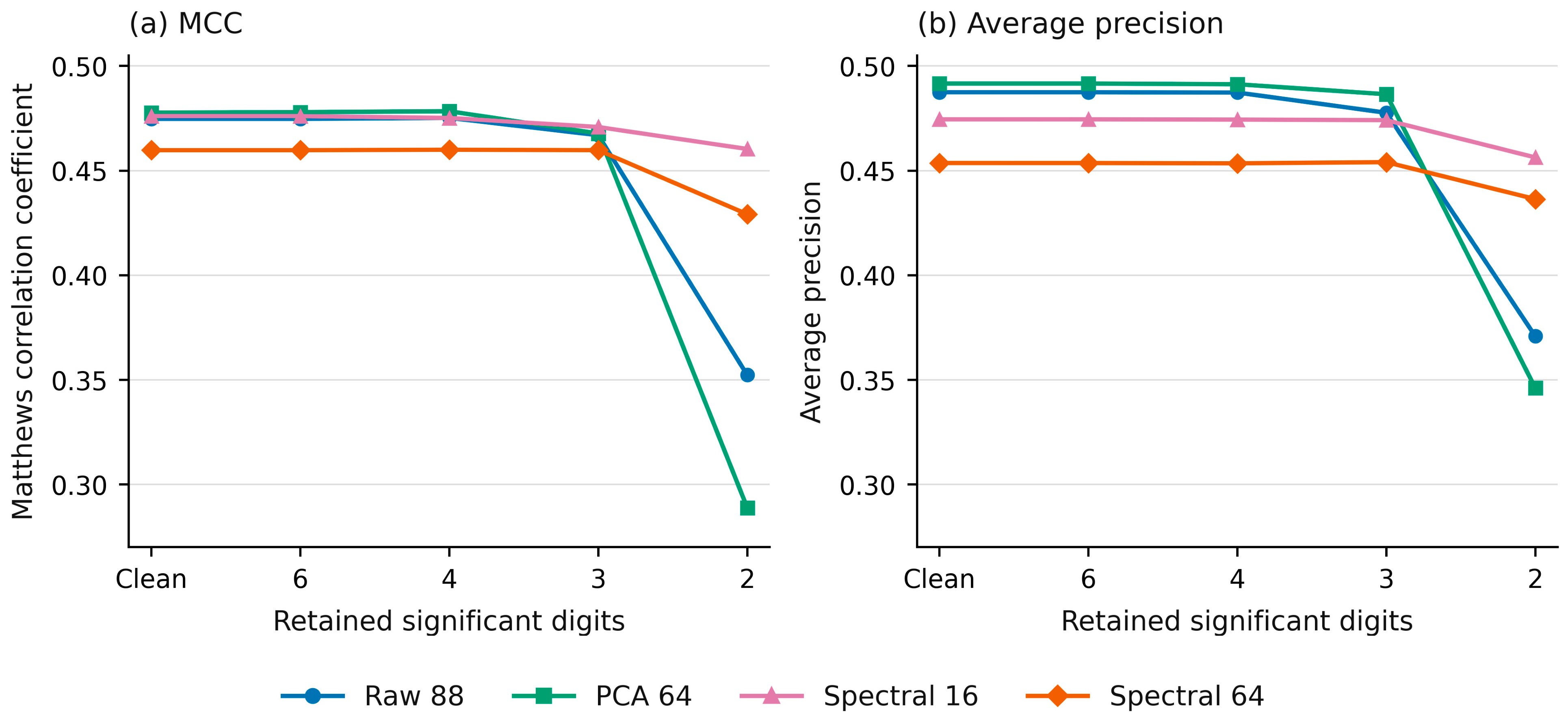
Figure A2.
Mean MCC loss from each model’s clean baseline across the full secondary severity grid for each corruption family. Lower loss denotes greater retention; negative values denote improvement in this finite scenario set. Families are not combined into an overall robustness score. Missingness, noise and annotation deletion average 1%, 5%, 10% and 20%; rounding averages 6, 4, 3 and 2 significant digits; block loss averages topology and biochemical removal. Absolute performance and all secondary contrasts are supplied.
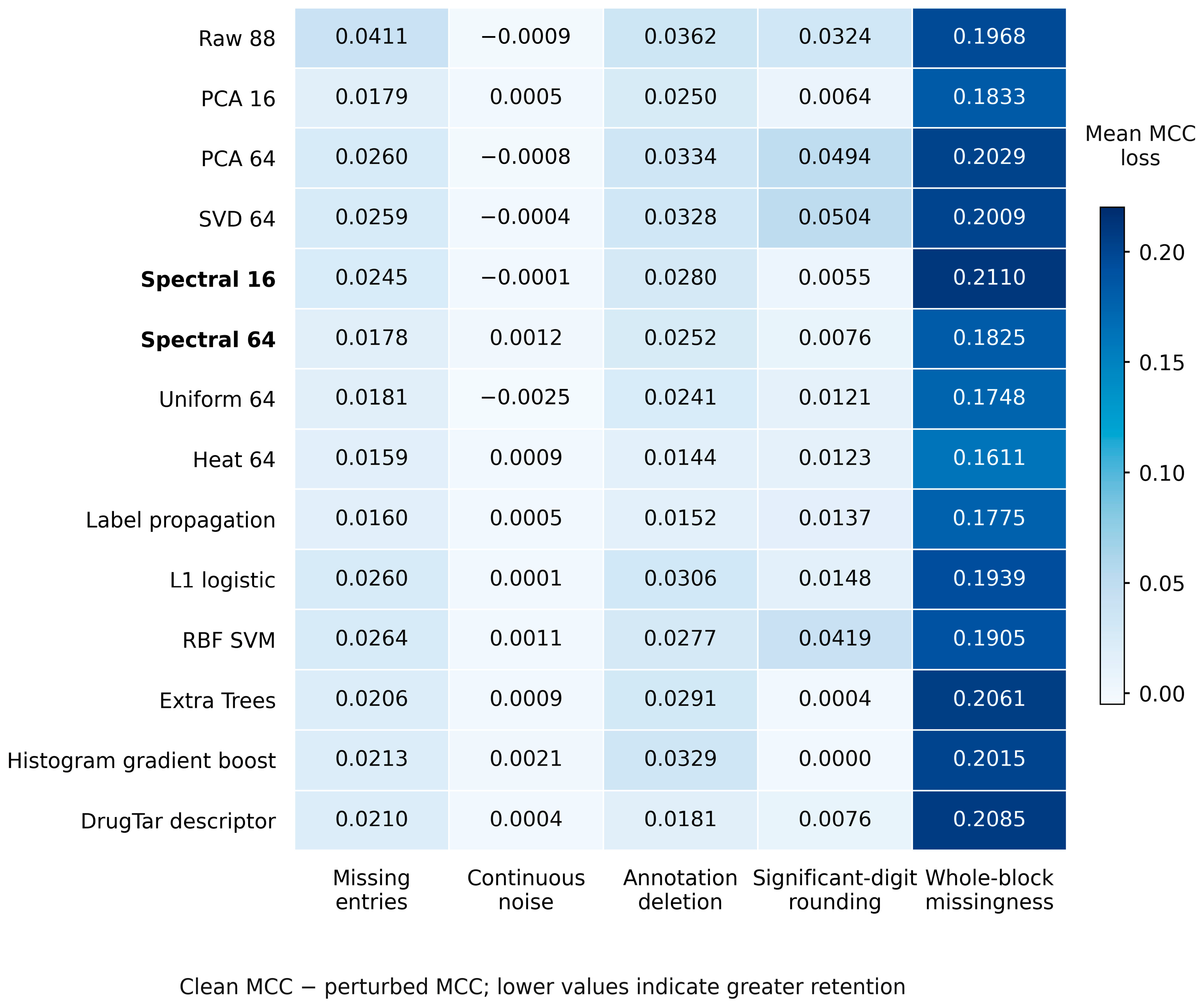
Appendix A.8.3. Conditional Analytical Stability Assessment
The mathematical domain is an unrestricted continuous L2 ball after frozen imputation and standardization, relaxing the real binary/discrete and biological input constraints. The fitted training graph, eigensystem, cached signals, classifier and threshold remain fixed. The calculation does not cover new missingness patterns, refitting, biological edits that change the true label, or numerical-platform errors. Part 2 supplied methodological context [50]; clause-level review used the supplied earlier DIS [53]. No claim of normative conformity follows.
For a fixed affine classifier, the exact distance to its selected decision boundary is |f(x) − θ|/‖βeff‖2, where βeff is the input-space SVM slope vector (component-matrix transpose times the SVM vector for PCA/SVD). For the nonlinear spectral map, a query perturbation with radius ρ < ‖x‖2 changes each cosine similarity by at most b = 2ρ/‖x‖2. A kth-to-(k + 1)th similarity gap γ > 2b preserves the top-k neighbor set. If S is the sum of retained positive cosine weights and S > kb, the normalized weight-vector change is bounded by 2kb/(S − kb) in L1 norm. This is multiplied by the maximum norm of each retained cached signal’s deviation from its clean weighted mean to bound the interaction change.
At each of the five updates, tanh non-expansiveness bounds the pre-normalization change e by the previous state bound plus α times the interaction bound. For N(v) = v/(‖v‖2 + ε), clean norm R and perturbation bound e, the next state bound is the minimum of 2, 2e/(R + ε), and e/(R − e + ε) when e < R. The final SVM coefficient norm converts the state bound to a score-change bound, which must remain strictly below |f(x) − θ|. A 40-step bisection finds an admissible radius with an interior factor of 0.999999. The derivation and runnable implementation are supplied. That factor does not replace validated floating-point arithmetic.
Table A30.
Conditional analytical radii in continuous standardized-input space. The final column is the percentage of all 9213 proteins that are clean-correct and stable by the available bound at radius 0.01. Exact affine distances and conservative spectral bounds differ in tightness and cannot establish an actual robustness ranking.
Thirty-seven queries per spectral arm had zero neighbor-boundary gaps and therefore inconclusive zero radii. Constant-score and zero-margin cases were handled explicitly. All saved clean scores were checked before bound calculation. The derivation received an independent mathematical check, and 4800 random synthetic perturbation probes plus tie, zero-query and boundary cases detected no implementation discrepancy; these probes are checks, not a formal proof. The isolated graph filter, uniform projector, PCA projector and raw identity all have operator norm one, so filter non-expansiveness alone cannot establish a unique spectral advantage. Reported correct-and-stable fractions intersect decision stability with clean correctness and are not MCC lower bounds.
References
- Santos, R.; Ursu, O.; Gaulton, A.; Bento, A.P.; Donadi, R.S.; Bologa, C.G.; Karlsson, A.; Al-Lazikani, B.; Hersey, A.; Oprea, T.I.; et al. A comprehensive map of molecular drug targets. Nat. Rev. Drug Discov. 2017, 16, 19–34. [Google Scholar] [CrossRef] [Scilit] [PubMed]
- Hopkins, A.L.; Groom, C.R. The druggable genome. Nat. Rev. Drug Discov. 2002, 1, 727–730. [Google Scholar] [CrossRef] [Scilit] [PubMed]
- Schenone, M.; Dančík, V.; Wagner, B.K.; Clemons, P.A. Target identification and mechanism of action in chemical biology and drug discovery. Nat. Chem. Biol. 2013, 9, 232–240. [Google Scholar] [CrossRef] [Scilit] [PubMed]
- Overington, J.P.; Al-Lazikani, B.; Hopkins, A.L. How many drug targets are there? Nat. Rev. Drug Discov. 2006, 5, 993–996. [Google Scholar] [CrossRef] [Scilit] [PubMed]
- Aleksander, S.A.; Balhoff, J.; Carbon, S.; Cherry, J.M.; Drabkin, H.J.; Ebert, D.; Feuermann, M.; Gaudet, P.; Harris, N.L.; Hill, D.P.; et al. The Gene Ontology knowledgebase in 2023. Genetics 2023, 224, iyad031. [Google Scholar] [CrossRef] [Scilit] [PubMed]
- Assenov, Y.; Ramírez, F.; Schelhorn, S.E.; Lengauer, T.; Albrecht, M. Computing topological parameters of biological networks. Bioinformatics 2008, 24, 282–284. [Google Scholar] [CrossRef] [Scilit] [PubMed]
- Keiser, M.J.; Setola, V.; Irwin, J.J.; Laggner, C.; Abbas, A.I.; Hufeisen, S.J.; Jensen, N.H.; Kuijer, M.B.; Matos, R.C.; Tran, T.B.; et al. Predicting new molecular targets for known drugs. Nature 2009, 462, 175–181. [Google Scholar] [CrossRef] [Scilit] [PubMed]
- Abedi, M.; Marateb, H.R.; Mohebian, M.R.; Aghaee-Bakhtiari, S.H.; Nassiri, S.M.; Gheisari, Y. Systems biology and machine learning approaches identify drug targets in diabetic nephropathy. Sci. Rep. 2021, 11, 23452. [Google Scholar] [CrossRef] [Scilit] [PubMed]
- Borhani, N.; Izadi, I.; Motahharynia, A.; Sheikholeslami, M.; Gheisari, Y. DrugTar improves druggability prediction by integrating large language models and gene ontologies. Bioinformatics 2025, 41, btaf360. [Google Scholar] [CrossRef] [Scilit] [PubMed]
- Elnaggar, A.; Heinzinger, M.; Dallago, C.; Rehawi, G.; Wang, Y.; Jones, L.; Gibbs, T.; Feher, T.; Angerer, C.; Steinegger, M.; et al. ProtTrans: Toward understanding the language of life through self-supervised learning. IEEE Trans. Pattern Anal. Mach. Intell. 2022, 44, 7112–7127. [Google Scholar] [CrossRef] [Scilit] [PubMed]
- Lin, Z.; Akin, H.; Rao, R.; Hie, B.; Zhu, Z.; Lu, W.; Smetanin, N.; Verkuil, R.; Kabeli, O.; Shmueli, Y.; et al. Evolutionary-scale prediction of atomic-level protein structure with a language model. Science 2023, 379, 1123–1130. [Google Scholar] [CrossRef] [Scilit] [PubMed]
- Santagati, R.; Aspuru-Guzik, A.; Babbush, R.; Degroote, M.; González, L.; Kyoseva, E.; Moll, N.; Oppel, M.; Parrish, R.M.; Rubin, N.C.; et al. Drug design on quantum computers. Nat. Phys. 2024, 20, 549–557. [Google Scholar] [CrossRef] [Scilit]
- Smaldone, A.M.; Shee, Y.; Kyro, G.W.; Xu, C.; Vu, N.P.; Dutta, R.; Farag, M.H.; Galda, A.; Kumar, S.; Kyoseva, E.; et al. Quantum machine learning in drug discovery: Applications in academia and pharmaceutical industries. Chem. Rev. 2025, 125, 5436–5460. [Google Scholar] [CrossRef] [Scilit] [PubMed]
- Zhou, Y.; Chen, J.; Cheng, J.; Cao, X.; Zhang, Y.; Karemore, G.; Zitnik, M.; Chong, F.T.; Liu, J.; Fu, T.; et al. Quantum-machine-assisted drug discovery. npj Drug Discov. 2026, 3, 1. [Google Scholar] [CrossRef] [Scilit] [PubMed]
- Avramouli, M.; Savvas, I.K.; Vasilaki, A.; Garani, G. Unlocking the potential of quantum machine learning to advance drug discovery. Electronics 2023, 12, 2402. [Google Scholar] [CrossRef] [Scilit]
- Pyrkov, A.; Aliper, A.; Bezrukov, D.; Lin, Y.C.; Polykovskiy, D.; Kamya, P.; Ren, F.; Zhavoronkov, A. Quantum computing for near-term applications in generative chemistry and drug discovery. Drug Discov. Today 2023, 28, 103675. [Google Scholar] [CrossRef] [Scilit] [PubMed]
- Li, W.; Yin, Z.; Li, X.; Ma, D.; Yi, S.; Zhang, Z.; Zou, C.; Bu, K.; Dai, M.; Yue, J.; et al. A hybrid quantum computing pipeline for real world drug discovery. Sci. Rep. 2024, 14, 16942. [Google Scholar] [CrossRef] [Scilit] [PubMed]
- Liu, J.; Wang, H.; Sun, Y.; Fu, C.; Guo, J. Real-coded quantum-inspired genetic algorithm-based BP neural network algorithm. Math. Probl. Eng. 2015, 2015, 571295. [Google Scholar] [CrossRef] [Scilit]
- Li, Y.; Xiao, J.; Chen, Y.; Jiao, L. Evolving deep convolutional neural networks by quantum behaved particle swarm optimization with binary encoding for image classification. Neurocomputing 2019, 362, 156–165. [Google Scholar] [CrossRef] [Scilit]
- Balicki, J. Multi-objective quantum-inspired genetic algorithm for supervised learning of deep classification models. In Computational Science—ICCS 2023; Lecture Notes in Computer Science; Springer: Cham, Switzerland, 2023; Volume 14077, pp. 246–253. [Google Scholar] [CrossRef] [Scilit]
- Malik, S.; Patro, S.G.K.; Mahanty, C.; Lasisi, A.; Naveed, Q.N.; Buradi, A.; Emma, A.F.; Kumar, S.; Mubarakali, A. Quantum-inspired gravitationally guided particle swarm optimization for feature selection and classification. Sci. Rep. 2025, 15, 34155. [Google Scholar] [CrossRef] [Scilit] [PubMed]
- Shuman, D.I.; Narang, S.K.; Frossard, P.; Ortega, A.; Vandergheynst, P. The emerging field of signal processing on graphs: Extending high-dimensional data analysis to networks and other irregular domains. IEEE Signal Process. Mag. 2013, 30, 83–98. [Google Scholar] [CrossRef] [Scilit]
- Hammond, D.K.; Vandergheynst, P.; Gribonval, R. Wavelets on graphs via spectral graph theory. Appl. Comput. Harmon. Anal. 2011, 30, 129–150. [Google Scholar] [CrossRef] [Scilit]
- Kang, Q.; Zhao, K.; Song, Y.; Wang, S.; Tay, W.P. Node embedding from neural Hamiltonian orbits in graph neural networks. In Proceedings of the 40th International Conference on Machine Learning, PMLR, Honolulu, HI, USA, 23–29 July 2023; Volume 202, pp. 15786–15808. [Google Scholar]
- Williams, C.K.I.; Seeger, M. Using the Nyström method to speed up kernel machines. Adv. Neural Inf. Process. Syst. 2001, 13, 682–688. [Google Scholar]
- Varma, S.; Simon, R. Bias in error estimation when using cross-validation for model selection. BMC Bioinform. 2006, 7, 91. [Google Scholar] [CrossRef] [Scilit] [PubMed]
- Cawley, G.C.; Talbot, N.L.C. On over-fitting in model selection and subsequent selection bias in performance evaluation. J. Mach. Learn. Res. 2010, 11, 2079–2107. [Google Scholar]
- Joeres, R.; Blumenthal, D.B.; Kalinina, O.V. Data splitting to avoid information leakage with DataSAIL. Nat. Commun. 2025, 16, 3337. [Google Scholar] [CrossRef] [Scilit] [PubMed]
- Rao, R.; Bhattacharya, N.; Thomas, N.; Duan, Y.; Chen, X.; Canny, J.; Abbeel, P.; Song, Y.S. Evaluating protein transfer learning with TAPE. Adv. Neural Inf. Process. Syst. 2019, 32, 9689–9701. [Google Scholar] [PubMed]
- Steinegger, M.; Söding, J. MMseqs2 enables sensitive protein sequence searching for the analysis of massive data sets. Nat. Biotechnol. 2017, 35, 1026–1028. [Google Scholar] [CrossRef] [Scilit] [PubMed]
- The UniProt Consortium. UniProt: The Universal Protein Knowledgebase in 2023. Nucleic Acids Res. 2023, 51, D523–D531. [Google Scholar] [CrossRef] [Scilit] [PubMed]
- Chung, F.R.K. Spectral Graph Theory; American Mathematical Society: Providence, RI, USA, 1997. [Google Scholar]
- von Luxburg, U. A tutorial on spectral clustering. Stat. Comput. 2007, 17, 395–416. [Google Scholar] [CrossRef] [Scilit]
- Shuman, D.I.; Wiesmeyr, C.; Holighaus, N.; Vandergheynst, P. Spectrum-adapted tight graph wavelet and vertex-frequency frames. IEEE Trans. Signal Process. 2015, 63, 4223–4235. [Google Scholar] [CrossRef] [Scilit]
- Coifman, R.R.; Lafon, S. Diffusion maps. Appl. Comput. Harmon. Anal. 2006, 21, 5–30. [Google Scholar] [CrossRef] [Scilit]
- Kondor, R.I.; Lafferty, J.D. Diffusion kernels on graphs and other discrete input spaces. In Proceedings of the 19th International Conference on Machine Learning, Sydney, Australia, 8–12 July 2002; pp. 315–322. [Google Scholar]
- Cortes, C.; Vapnik, V. Support-vector networks. Mach. Learn. 1995, 20, 273–297. [Google Scholar] [CrossRef] [Scilit]
- Fan, R.E.; Chang, K.W.; Hsieh, C.J.; Wang, X.R.; Lin, C.J. LIBLINEAR: A library for large linear classification. J. Mach. Learn. Res. 2008, 9, 1871–1874. [Google Scholar]
- Jolliffe, I.T.; Cadima, J. Principal component analysis: A review and recent developments. Philos. Trans. R. Soc. A 2016, 374, 20150202. [Google Scholar] [CrossRef] [Scilit] [PubMed]
- Halko, N.; Martinsson, P.G.; Tropp, J.A. Finding structure with randomness: Probabilistic algorithms for constructing approximate matrix decompositions. SIAM Rev. 2011, 53, 217–288. [Google Scholar] [CrossRef] [Scilit]
- Zhou, D.; Bousquet, O.; Lal, T.N.; Weston, J.; Schölkopf, B. Learning with local and global consistency. Adv. Neural Inf. Process. Syst. 2004, 16, 321–328. [Google Scholar]
- Chicco, D.; Jurman, G. The advantages of the Matthews correlation coefficient (MCC) over F1 score and accuracy in binary classification evaluation. BMC Genom. 2020, 21, 6. [Google Scholar] [CrossRef] [Scilit] [PubMed]
- Fawcett, T. An introduction to ROC analysis. Pattern Recognit. Lett. 2006, 27, 861–874. [Google Scholar] [CrossRef] [Scilit]
- Saito, T.; Rehmsmeier, M. The precision-recall plot is more informative than the ROC plot when evaluating binary classifiers on imbalanced datasets. PLoS ONE 2015, 10, e0118432. [Google Scholar] [CrossRef] [Scilit] [PubMed]
- Efron, B. Bootstrap methods: Another look at the jackknife. Ann. Stat. 1979, 7, 1–26. [Google Scholar] [CrossRef] [Scilit]
- Schuirmann, D.J. A comparison of the two one-sided tests procedure and the power approach for assessing the equivalence of average bioavailability. J. Pharmacokinet. Biopharm. 1987, 15, 657–680. [Google Scholar] [CrossRef] [Scilit] [PubMed]
- Lakens, D. Equivalence tests: A practical primer for t tests, correlations, and meta-analyses. Soc. Psychol. Personal. Sci. 2017, 8, 355–362. [Google Scholar] [CrossRef] [Scilit] [PubMed]
- Pedregosa, F.; Varoquaux, G.; Gramfort, A.; Michel, V.; Thirion, B.; Grisel, O.; Blondel, M.; Prettenhofer, P.; Weiss, R.; Dubourg, V.; et al. Scikit-learn: Machine learning in Python. J. Mach. Learn. Res. 2011, 12, 2825–2830. [Google Scholar]
- ISO/IEC TR 24029-1:2021; Artificial Intelligence (AI)—Assessment of the Robustness of Neural Networks—Part 1: Overview. ISO: Geneva, Switzerland, 2021.
- ISO/IEC 24029-2:2023; Artificial Intelligence (AI)—Assessment of the Robustness of Neural Networks—Part 2: Methodology for the Use of Formal Methods. ISO: Geneva, Switzerland, 2023.
- ISO/IEC DIS 24029-3; Artificial Intelligence (AI)—Assessment of the Robustness of Neural Networks—Part 3: Methodology for the Use of Statistical Methods. Draft International Standard, Enquiry Text; ISO: Geneva, Switzerland, 2026; Official Project Status: FDIS, Under Development. Available online: https://committee.iso.org/standard/86901.html (accessed on 1 November 2026).
- Holm, S. A simple sequentially rejective multiple test procedure. Scand. J. Stat. 1979, 6, 65–70. [Google Scholar]
- ISO/IEC DIS 24029-2; Artificial Intelligence (AI)—Assessment of the Robustness of Neural Networks—Part 2: Methodology for the Use of Formal Methods. ISO: Geneva, Switzerland, 2022.
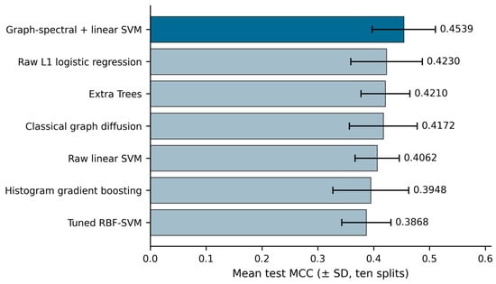
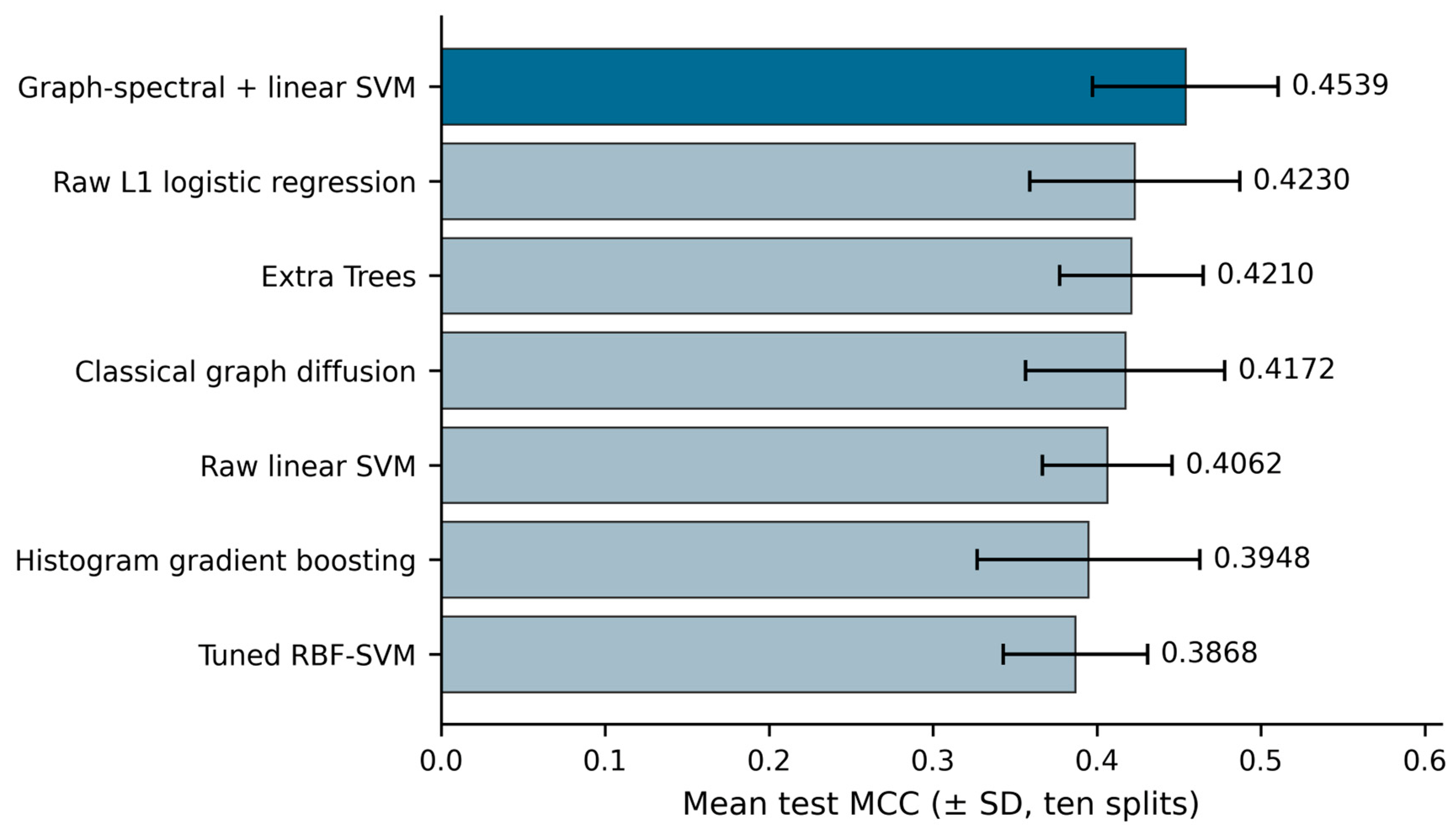
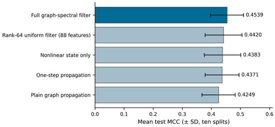
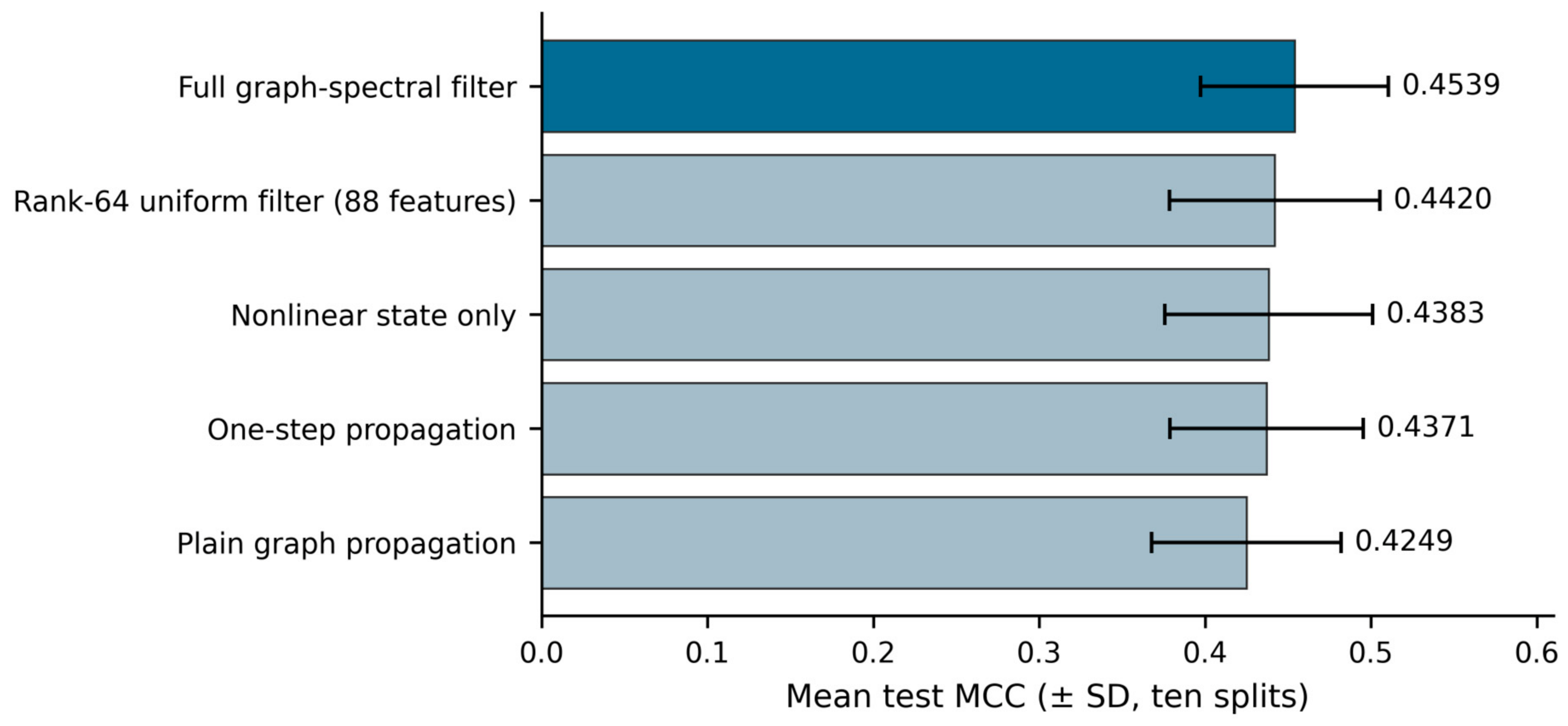
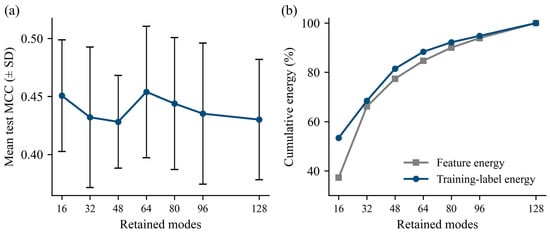
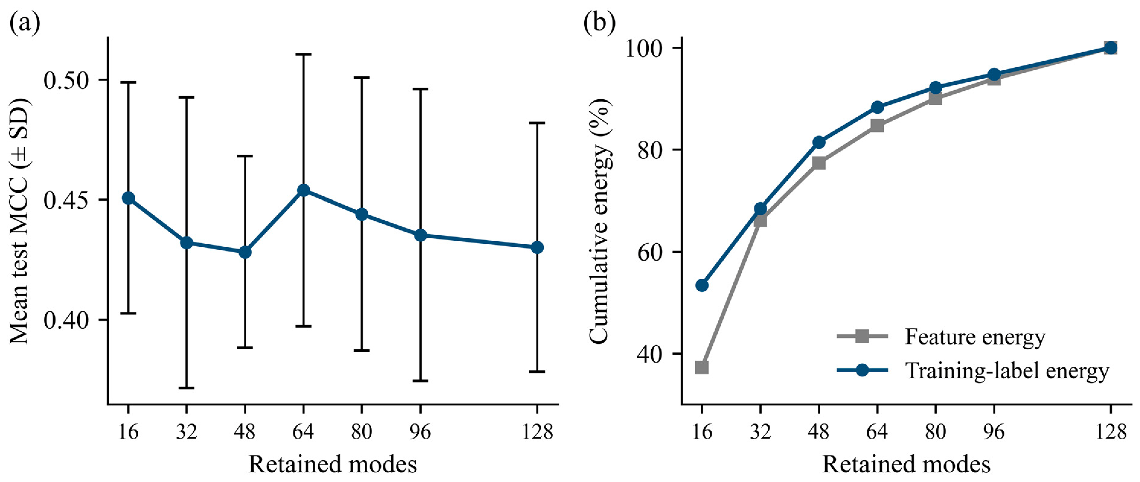
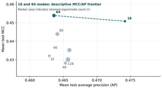
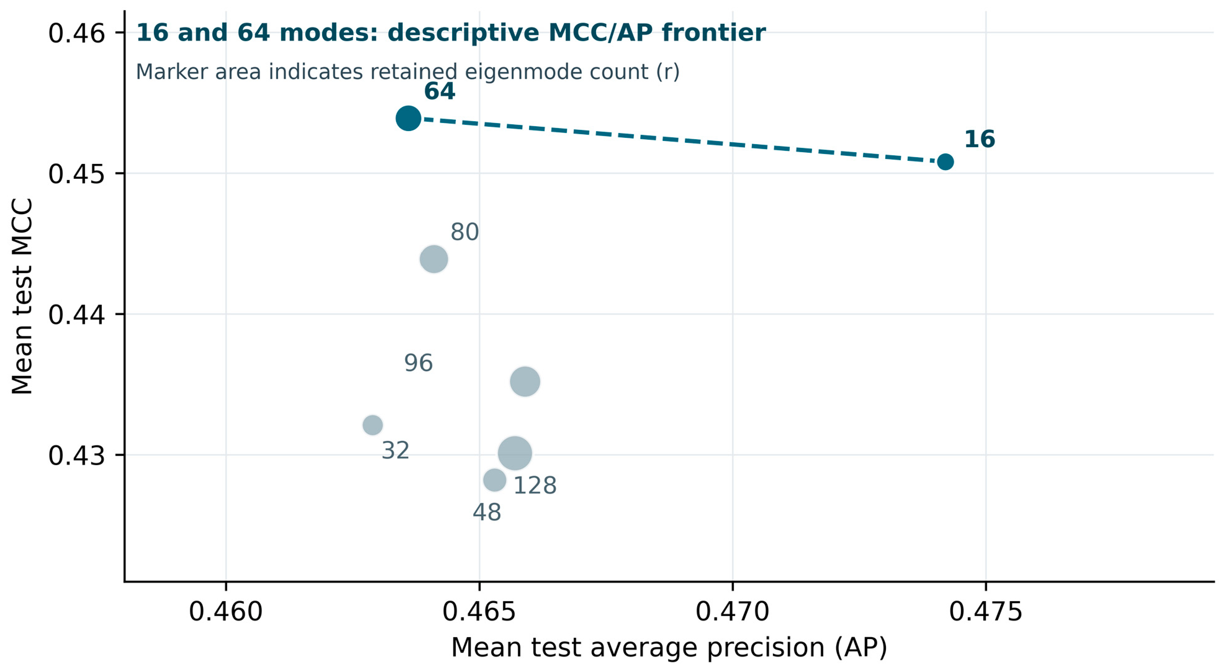
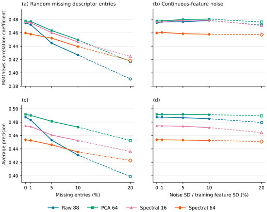
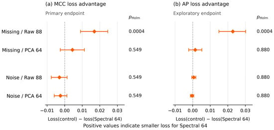

Disclaimer/Publisher’s Note: The statements, opinions and data contained in all publications are solely those of the individual author(s) and contributor(s) and not of MDPI and/or the editor(s). MDPI and/or the editor(s) disclaim responsibility for any injury to people or property resulting from any ideas, methods, instructions or products referred to in the content. |
© 2026 by the authors. Licensee MDPI, Basel, Switzerland. This article is an open access article distributed under the terms and conditions of the Creative Commons Attribution (CC BY) license.