


Abstract
Background: Deep learning systems for diabetic retinopathy (DR) grading are usually reported through accuracy and area under the curve, yet clinical use depends on whether a model’s confidence can be trusted. Problem: calibration and confidence-based triage are rarely evaluated on large, naturally imbalanced five-grade datasets. Objective: to quantify how temperature scaling and Monte Carlo (MC) Dropout change the reliability of an EfficientNet-B0 DR grader and to convert calibrated confidence into auto-clear/human-review operating points. Materials: A total of 12,522 DDR fundus photographs on the five ICDR grades, only 1.9% of them severe non-proliferative DR. Methods: Methods included five-fold cross-validation grouped by near-duplicate images, with inner calibration splits; overall and per-grade expected calibration error (ECE); clustered bootstrap; comparison with other calibration maps, loss functions and backbones; Grad-CAM and LIME. Results: Macro-F1 was 0.705 (95% CI 0.691–0.718). Temperature scaling reduced ECE from 0.186 to 0.078 without changing any prediction, but grade-specific maps were needed to bring per-grade ECE below 0.01. Mutual information from MC-Dropout flagged errors better than confidence (AUROC 0.748 vs. 0.650). At a no-DR threshold of 0.80, 30.1% of images were auto-cleared with a 1.46% referable-DR false-clear rate. Conclusions: One temperature corrected most top-label miscalibration but not the grade-level error caused by class weighting; the triage thresholds need external validation before clinical use.
1. Introduction
1.1. Background
Diabetic retinopathy (DR) is the leading cause of preventable blindness among working-age adults worldwide, and its prevalence continues to rise in step with the global burden of diabetes mellitus [1,2]. Treatment works best when retinopathy is caught early, because laser photocoagulation, anti-VEGF injections and timely referral can all stop sight-threatening progression. The difficulty is volume. Hundreds of millions of people with diabetes should be photographed every year, and there are far too few ophthalmologists and trained graders to read those images, a shortage felt most in low- and middle-income countries. This capacity gap has motivated more than a decade of intensive research into automated, deep-learning-based DR screening, with convolutional neural networks (CNNs) now routinely reported to match or exceed human-grader agreement on binary referable/non-referable screening tasks and, increasingly, on the finer-grained five-class International Clinical Diabetic Retinopathy (ICDR) severity scale (no DR; mild, moderate, and severe non-proliferative DR; and proliferative DR) [3,4,5]. Prospective deployment within national screening programmes has also been reported [6], and retinal foundation models pretrained on very large unlabelled image collections now extend these results across several ocular and systemic conditions [7].
The apparent success of these systems, however, is disproportionately reported through a narrow lens: an aggregate accuracy or area-under-the-curve (AUC) figure computed on a single train/test split, frequently on a class-balanced or near-balanced benchmark. This convention hides two features of real screening data. The first is imbalance. Most screened eyes have no retinopathy or only mild disease, and the severe and proliferative cases that a programme exists to find are uncommon, so a model can post a high overall accuracy and still do poorly on the grades that matter. The second is that an accuracy figure says nothing about whether the model recognises its own mistakes. A classifier that outputs a 99% confident but wrong prediction is, from a deployment-safety standpoint, categorically worse than one that outputs the same wrong prediction with 55% confidence and is consequently flagged for human review. This property, whether a model’s predicted confidence is a trustworthy estimate of its probability of being correct, is called calibration [8,9], and it is largely absent from the DR-grading literature, which continues to report classification metrics computed on raw, uncalibrated softmax outputs.
1.2. Problem Statement
We see three gaps. (i) Calibration is seldom measured. Deep networks are known to be miscalibrated, usually over-confident, as a by-product of the depth, normalisation, label smoothing and long training that make them accurate [9,10], yet DR papers report accuracy, sensitivity, specificity and AUC far more often than expected calibration error (ECE), the Brier score or a reliability diagram. (ii) Uncertainty quantification is treated as a niche add-on rather than an integral evaluation axis. Where uncertainty is reported at all, it is typically demonstrated qualitatively on a handful of sample images rather than benchmarked, at the full test-set level, against the specific clinical question of how many cases can be safely auto-cleared without human review [11,12]. (iii) Imbalance is mentioned in most papers but seldom examined with macro-averaged metrics, per-class results and resampling-based intervals together. Studies that do report per-class metrics seldom couple them with confidence intervals wide enough to communicate the genuine statistical uncertainty introduced by rare classes such as severe non-proliferative DR, which in the dataset used here constitutes under 2% of all images [13].
Collectively, these gaps mean that a clinician, health system, or regulator reading a typical DR-grading paper cannot answer the question that actually determines whether the system is deployable: at what confidence threshold can this model’s output be trusted enough to skip human review, and how many sight-threatening cases would be missed at that threshold?
Parts of this question have been studied before; the whole of it has not. Uncertainty-based referral in DR has been studied for the binary referable/non-referable decision [14,15,16]; those studies show that referring uncertain cases improves accuracy on the retained cases, but they do not report whether the probabilities themselves are calibrated, nor how many images could be released without review at a stated false-clear rate. Calibration studies in medical imaging [17] usually report a single top-label ECE, which cannot show whether rare grades are calibrated, and they rarely ask how the remedy chosen for class imbalance changes calibration. Finally, DR studies almost never state whether images of the same eye can fall on both sides of a train/test split, a point that affects every number reported. It therefore remains unknown how calibration, uncertainty and an auto-clear rule behave together on an imbalanced five-grade task, and which of the available tools is responsible for which part of the reliability gain.
1.3. Objective and Contributions
This study addresses the gap directly by conducting a class-imbalance-aware, calibration-centred evaluation of a convolutional DR-grading pipeline on the DDR dataset, a large, publicly available, naturally imbalanced five-class ICDR grading benchmark. Rather than proposing a new architecture, the contribution of this work is methodological and evaluative, in line with the TRIPOD + AI recommendation that calibration be reported alongside discrimination [18]: a rigorous, statistically grounded protocol for calibration, uncertainty quantification, triage-oriented deployment analysis, and dual explainability, applied under stratified five-fold cross-validation with bootstrap confidence intervals throughout. Concretely, this paper contributes the following:
- A five-fold cross-validation benchmark, stratified by grade and built from groups of near-duplicate images, of an EfficientNet-B0 DR-grading classifier on 12,522 DDR images, reporting the full complement of discrimination metrics (accuracy, macro-/micro-/weighted-F1, balanced accuracy, MCC, per-class precision/recall/specificity, ROC-AUC, and PR-AUC) alongside group-clustered bootstrap 95% confidence intervals, per-grade intervals and fold-level variability statistics.
- A paired ablation of three inference-time confidence strategies (raw softmax, post hoc temperature-scaled softmax, and temperature-scaled Monte Carlo Dropout) applied to the same trained weights, with paired bootstrap confidence intervals and McNemar’s test isolating how much of the reliability gain comes from single-parameter rescaling versus stochastic forward-pass uncertainty estimation. Temperature scaling is further compared with vector scaling, Dirichlet calibration and isotonic regression are fitted on the same calibration split.
- A confidence-stratified triage curve that converts calibrated confidence into an operational quantity: the fraction of images that could be auto-cleared at a given threshold, together with the referable-DR and any-DR miss rates within the auto-cleared subset. Few DR-grading studies report this, although it is the number a screening service needs. Each operating point is reported with Wilson and clustered-bootstrap confidence intervals, per-fold values, and a threshold chosen on the calibration split and tested on the outer fold.
- Grad-CAM, a gradient-based saliency method, and LIME, a model-agnostic local surrogate, applied to a systematic sample of correct and misclassified images from every grade, with measured stability, faithfulness and agreement between the two.
- A paired training-recipe comparison on the same folds (plain, focal and class-balanced cross-entropy, oversampling, early stopping, and ResNet-50 and ViT-B/16 backbones), showing how the imbalance remedy trades discrimination, calibration and triage safety against one another.
- A transparent accounting of what this study does not claim: no structured clinical metadata (age, HbA1c, blood pressure, body-mass index) were available for the DDR cohort, and no synthetic metadata were fabricated to simulate a multimodal fusion pipeline; the metadata-conditioned Shapley-value analysis originally scoped for a cross-attention fusion architecture is consequently reported as not applicable in this data release and is explicitly deferred to future work pending access to a retinal-imaging cohort with genuine linked systemic clinical variables (Section 6.2).
We do not claim that temperature scaling, MC-Dropout, Grad-CAM or LIME is new, and integration alone is not offered as the contribution. What the paired design adds is a set of measured findings that earlier DR studies did not report. Three findings follow from it. Because the confidence variants share weights and folds, each change can be traced to one tool: on DDR, a single temperature removes most top-label miscalibration, the rare grades need class-specific maps, and MC-Dropout helps to rank errors but not calibrate. The training-recipe comparison then shows that class weighting, the usual way of protecting rare grades, is itself the main cause of grade-level miscalibration, even though it gives the safest auto-clear rule; which post hoc step a programme needs depends on this trade-off. Finally, the triage results give the workload and false-clear rate of a five-grade output with intervals, a threshold chosen on separate data, and the ceiling of the no-DR probability that caps automation for this model. These are observations about known methods on an imbalanced five-grade task, not a new algorithm.
1.4. Structure of the Paper
Section 2 reviews work on DR grading, calibration, uncertainty estimation, explainability and selective classification. Section 3 describes the data, the grouped cross-validation, the network and its training, the calibration and uncertainty methods, the statistics, the explanation methods and how cost was measured. Section 4 gives the results: training behaviour, discrimination, calibration, triage, errors, explanations, variability and cost. Section 5 contains the ablations, covering the three confidence variants, other calibration maps, the number of MC-Dropout passes, and other training recipes and backbones. Section 6 states the conclusions, limitations and future work. The Supplementary Materials hold the fold-level tables, calibration bins, the full triage table, all explanation panels and the files needed to reproduce the analysis.
2. Related Work
2.1. Deep Learning for Diabetic Retinopathy Grading
Gulshan et al. [3] were the first to show that a convolutional network could detect referable DR as well as ophthalmologists; they trained Inception-v3 on a large private set of adjudicated photographs and tested it on several independent sets. Gargeya and Leng [19] and Ting et al. [4] subsequently reported comparably strong discrimination on binary and multi-class formulations using deep residual and Inception-family architectures across multi-ethnic screening cohorts. Public datasets such as EyePACS/APTOS, Messidor-2, IDRiD and DDR later made it possible to repeat such work and to compare architectures directly. Li et al. [13] introduced the DDR dataset specifically to address a limitation of earlier benchmarks: DDR combines ICDR severity grading with lesion-level segmentation annotations from Chinese screening centres, and its class distribution is left deliberately unrebalanced, making it one of the more realistic large-scale public benchmarks for studying imbalance-aware DR grading. The EfficientNet family of Tan and Le [20], scaled jointly in depth, width and resolution, is now widely used for DR grading because it gives more accuracy per FLOP than VGG- or ResNet-style networks, which is why we use EfficientNet-B0. Other groups have gone beyond retrospective image-level grading. Dai et al. [5] developed a system that detects DR across the full severity spectrum with lesion-aware sub-networks trained on large screening cohorts, Ruamviboonsuk et al. [6] reported a prospective, multisite evaluation of real-time screening in a national programme, and Zhou et al. [7] introduced RETFound, a self-supervised foundation model for retinal images that improves label efficiency across ocular and systemic prediction tasks. Vision transformers [21], the encoder used by RETFound, and EfficientNetV2 [22] are further options, both more costly to run than EfficientNet-B0. Lightweight detectors aimed at the small lesions of early DR [23], portable screening and grading systems built for use outside specialist centres, as shown for glaucoma [24], and external validation of severity grading and referable-risk stratification on independent fundus data [25] continue this move toward practical use.
Even so, most DR-grading papers give one accuracy or AUC figure per model, from one held-out split, with no cross-validated spread, no per-class intervals and, most importantly here, no check of whether the softmax probabilities are calibrated. Two models with the same AUC can behave quite differently once their confidence is used to decide which images a person must read, as it is in any triage workflow. Published results are also hard to compare directly. Some studies used large, privately adjudicated datasets with external test sets [3,4], while others reported results on public benchmarks with a single split [13,19]. Endpoints range from binary referable DR to the full five-grade scale, ungradable images are handled in different ways, and few papers state whether images of one patient or eye were kept on one side of the split. An accuracy figure from one design therefore cannot be set beside one from another; calibration and per-grade results travel better between designs.
2.2. Calibration of Deep Neural Network Classifiers
Guo et al. [9] demonstrated, across a range of modern image-classification architectures, that increasing network depth and width, the trend that has driven accuracy improvements over the past decade, has been accompanied by a corresponding worsening of calibration, with deep networks becoming systematically overconfident even as their raw accuracy improves. They also showed that temperature scaling, which divides the logits by one scalar fitted on a held-out split, removes most of this error. Because the transformation is monotonic it cannot move the arg-max, so predictions and discrimination metrics are untouched. Temperature scaling has since become the baseline against which Platt scaling, isotonic regression, Dirichlet calibration and focal-loss training are judged. Calibration failures have been reported for dermoscopy, chest radiograph and histopathology classifiers, but for DR grading, ECE and the Brier score are still rarely given next to discrimination. Minderer et al. [10] found that architecture matters a great deal, with vision transformers among the best-calibrated recent models, and focal loss [26] can improve calibration during training without any post hoc step. In medical imaging, Rajaraman et al. [17] reported that calibrating models trained on class-imbalanced data improved their performance at the decision threshold, while Van Calster et al. [8] argued that poorly calibrated risk estimates can mislead clinical decisions even when discrimination is high.
These methods differ in what they can and cannot correct. Temperature scaling has one parameter, so it cannot overfit a small calibration set, but it applies the same correction to every class and cannot repair class-specific miscalibration. Vector scaling, matrix scaling and Dirichlet calibration [27] learn class-specific corrections, at the price of 2K to K2 + K parameters that must be estimated from the calibration split; with rare grades, this is a real constraint. Isotonic regression [28] is non-parametric and flexible, but it needs more data per class and produces step-shaped probability maps. Training-time approaches such as focal loss [26,29] or class-balanced loss [30] change the classifier itself, so their effect on calibration cannot be separated from their effect on discrimination. How calibration is measured also matters. Equal-width ECE changes with the number of bins and is biased when bins hold few samples, and top-label ECE ignores every class except the predicted one [31]. With five grades and heavy imbalance, a small top-label ECE can sit alongside badly calibrated probabilities for the rare grades. We come back to both issues in Section 4.5 and Section 5.5.
2.3. Uncertainty Quantification via Monte Carlo Dropout and Deep Ensembles
Uncertainty quantification methods for deep networks have been reviewed extensively [11,12]. Gal and Ghahramani [32] showed that dropout, first proposed as a regulariser, can be read as approximate Bayesian inference: if dropout stays on at test time and the image is passed through the network several times, the passes form a Monte Carlo sample of the predictive distribution. Its mean gives the prediction and its spread or entropy the epistemic uncertainty, at a small fraction of the cost of a full Bayesian network or an ensemble. Lakshminarayanan et al. [33] proposed deep ensembles, in which several independently initialised networks are trained, as a competing, typically better-calibrated but substantially more computationally expensive alternative. The present study adopts MC-Dropout specifically because its computational overhead (a configurable number of stochastic forward passes through a single trained network) is far more compatible with the deployment latency budget realistic for a screening tool than training and maintaining an ensemble of independently trained networks, while still yielding a usable per-image uncertainty signal; the entropy and mutual-information decompositions used here follow the standard MC-Dropout formulation summarised in Section 3.6. Ovadia et al. [34] later found deep ensembles to be the most reliable of the methods they compared under dataset shift. In DR specifically, Leibig et al. [14] showed that referring the most uncertain MC-Dropout predictions for expert review improved performance on the retained cases, Ayhan et al. [15] found that model uncertainty was associated with expert-assessed diagnostic difficulty, and Band et al. [16] benchmarked Bayesian deep learning methods for DR detection under distribution shift. These studies established uncertainty-based referral for binary DR detection but did not evaluate calibration and triage jointly on a five-grade task or isolate the contribution of MC-Dropout relative to temperature scaling.
The methods above also differ in which part of the model’s uncertainty they capture. Deep ensembles sample over complete, independently trained networks. MC-Dropout samples only over the layers that contain dropout, so its estimate depends on where dropout is placed. Test-time augmentation measures sensitivity to input perturbation rather than to the weights. None of these methods guarantees good calibration after a change of camera, population or image quality: Ovadia et al. [34] and Band et al. [16] found that calibration and uncertainty quality degraded under dataset shift for every method tested, with ensembles degrading least. The results of the present study therefore describe in-distribution behaviour on DDR and are not evidence of calibration after deployment elsewhere.
2.4. Explainability in Medical Image Classification
Grad-CAM, proposed by Selvaraju et al. [35], produces a coarse, class-discriminative localisation map by weighting the final convolutional feature maps by the gradient of the target class score with respect to those feature maps, and has become a near-default sanity check for CNN-based medical image classifiers because it is architecture-agnostic (requiring only that the network expose convolutional feature maps) and requires no retraining. LIME, proposed by Ribeiro et al. [36], instead perturbs interpretable input components (superpixels, in the image domain) and fits a local, inherently interpretable surrogate model (typically sparse linear regression) to the perturbed predictions, yielding a locally faithful but model-agnostic explanation together with a goodness-of-fit statistic (R2) that Grad-CAM does not provide. Prior DR-grading studies have applied one or the other of these methods, almost always Grad-CAM alone, to illustrate that the network attends to lesion-bearing retinal regions (microaneurysms, haemorrhages, exudates, neovascularisation) rather than spurious image artefacts. Evaluations of saliency methods in medical imaging have found that heatmaps often localise abnormalities less accurately than human annotations and can fail randomisation and repeatability tests [37,38], and a review of explainable AI in medical image analysis identified the limited evaluation of explanation quality as a central open problem [39]. The present study applies both methods on matched examples spanning all five ICDR grades, including a genuine misclassification, and additionally reports the LIME surrogate R2 per class as a quantitative, if indirect, proxy for how locally linear (and therefore how straightforwardly explainable) the network’s decision boundary is for each severity grade.
2.5. Retinal Foundation Models and Selective Classification
Retinal foundation models pre-trained on large unlabelled fundus collections, such as RETFound [7], have improved label efficiency and cross-dataset generalisation for DR and for other ocular and systemic conditions. Their published evaluations centre on discrimination across tasks and datasets; calibration and selective referral were not primary endpoints. Because larger pre-trained encoders are often better calibrated in-distribution than small convolutional networks [10], they are an obvious comparison for the calibration findings reported here, but they also cost far more computation per image (Section 4.11), and transformer backbones are known to need training recipes different from those of convolutional networks [21]. We therefore treat foundation-model backbones as an extension of the present paired design (Section 6.3) rather than as part of it.
Selective classification gives the triage question a formal frame. A selective classifier abstains on part of its input, and its quality is described by the risk–coverage curve: the error rate on accepted cases is a function of the fraction accepted [40]. In clinical work, the abstained cases go to a person. Deferral can also be learned so that model and clinician each handle the cases they do best [41], and how uncertainty is shown to the clinician is a design problem in itself [42]. Our triage rule is a one-sided selective classifier that accepts only images it judges normal; Section 4.6 gives both the threshold and the risk–coverage results.
2.6. Summary of Gaps and Motivation for the Present Study
In short, earlier work shows that deep CNNs, EfficientNet among them, discriminate DR grades well; that modern networks tend to be miscalibrated and that temperature scaling corrects much of this cost-effectively; that MC-Dropout gives per-image uncertainty at modest cost; and that Grad-CAM and LIME show different aspects of a network’s decisions. We did not find a study that tests all of these together, with stratified cross-validation, bootstrap intervals and per-class reporting on a large five-grade dataset with its natural imbalance, and that then turns calibrated confidence into a stated triage rule. That is the aim of the present work. Table 1 lists the main contribution of each reviewed study and its relation to ours.
Table 1.
Reviewed studies: what each contributed and how it relates to the present work.
3. Materials and Methods
Figure 1 outlines the six stages of the study. The input is the set of 12,522 graded DDR photographs (stage 1), which are cropped, resized, normalised and, for training only, augmented (stage 2). All experiments use five-fold cross-validation stratified by grade and built from groups of near-duplicate images, and each development partition is split again into inner training and calibration sets (stage 3). An EfficientNet-B0 classifier is trained on the inner training set (stage 4), and its logits are turned into three confidence estimates: raw softmax, temperature-scaled softmax and temperature-scaled MC-Dropout (stage 5). The pooled out-of-fold predictions are then evaluated for discrimination, calibration, statistical significance, explanations and cost, and the calibrated no-DR probability decides between auto-clearance and human review (stage 6). Section 3.1, Section 3.2, Section 3.3, Section 3.4, Section 3.5, Section 3.6, Section 3.7, Section 3.8, Section 3.9, Section 3.10, Section 3.11 and Section 3.12 describe each stage in turn.
Figure 1.
Proposed calibration- and triage-centred framework for five-grade DR assessment. (1) DDR fundus images; (2) preprocessing; (3) five-fold cross-validation, stratified by grade and grouped by near-duplicate images, with an inner calibration split, so that the outer test fold never influences training, monitoring, or temperature fitting; (4) EfficientNet-B0 classifier; (5) the three confidence-estimation variants compared in the ablation study; (6) evaluation of the pooled out-of-fold predictions, including the confidence-stratified triage rule that auto-clears an image when its no-DR probability is at or above the threshold τ.
3.1. Dataset and Preprocessing
This study uses the DDR (Diabetic Retinopathy grading) dataset [13], a publicly available collection of colour fundus photographs graded according to the five-level International Clinical Diabetic Retinopathy (ICDR) severity scale: grade 0 (no apparent DR), grade 1 (mild non-proliferative DR), grade 2 (moderate non-proliferative DR), grade 3 (severe non-proliferative DR), and grade 4 (proliferative DR). After the images marked ungradable in the dataset’s own quality labels were removed, 12,522 graded images remained. Table 2 and Figure 2 give the class counts. We kept the imbalance on purpose: grades 0 and 2 make up 85.8% of the data, whereas severe NPDR (grade 3), which matters clinically because it often progresses to proliferative disease, makes up only 1.9%.
Table 2.
Number of images per ICDR grade in the 12,522-image DDR set. The imbalance ratio between the most- and least-frequent class (grade 0 vs. grade 3) is 26.6:1.
Figure 2.
Class distribution of the 12,522 DDR images. No DR and moderate NPDR dominate, while mild and severe NPDR are rare, which is why the evaluation in this paper is built around class imbalance.
Before resizing, each fundus image was converted from BGR to RGB and cropped to the bounding box of pixels with grayscale intensity above 7 to remove the black border. All images were then brought to 384 × 384 pixels and normalised with ImageNet channel statistics (mean 0.485, 0.456, 0.406; standard deviation 0.229, 0.224, 0.225), matching the ImageNet-pretrained backbone. Stochastic geometric and photometric augmentation was applied on the fly to training images only, in the following order: random resized cropping to 384 × 384 (scale 0.85–1.0, aspect ratio 3/4–4/3), horizontal and vertical flipping (each with p = 0.5), random rotation within ±15°, and colour jitter (brightness and contrast factors in [0.88, 1.12], saturation factor in [0.92, 1.08], hue unchanged). Calibration-split and test-fold images received only deterministic resizing to 384 × 384 and normalisation. No test-time augmentation was used.
3.2. Cross-Validation Protocol
All results in this paper come from out-of-fold (OOF) predictions under five-fold cross-validation (k = 5). Folds were stratified on the five-level ICDR grade, so that each fold keeps the class ratio of Table 2, and were built from groups of near-duplicate images rather than from single images (described below), so that no group is split between training and testing. A fixed random seed (2026) governed the fold split, weight initialisation and augmentation sampling. Within each round, the four development folds were split again, by group and stratified by grade, into an inner training partition (8585–8586 images) and an inner calibration partition (1431 images; Supplementary Table S2); the held-out outer fold (2504–2505 images) served only as the test partition. The inner calibration partition was used for epoch-level monitoring, for fitting the temperature and the other calibration maps (Section 3.5 and Section 5.5), and for choosing a triage threshold in the sensitivity analysis of Section 4.6, so the outer test fold never influenced training, monitoring or calibration. Because every image belongs to exactly one outer test fold, concatenating the five test-fold predictions yields one OOF prediction for each of the 12,522 images, produced by a model that saw neither that image nor any near-duplicate of it. All pooled metrics in Section 4 are computed on this OOF set (Supplementary Data S1, with the split assignments in Data S2) unless stated as fold-level or bootstrap statistics.
DDR releases an image identifier and a grade for each image but no patient identifier, and the original description reports 13,673 images from 9598 patients [13], so some patients contribute more than one image. Since a split by patient was not possible, we removed the most direct source of leakage, which is repeated or near-identical photographs of the same eye. Each image was reduced to two 256-bit perceptual hashes (a DCT-based pHash and a gradient-based dHash) computed on the high-pass-filtered green channel of the border-cropped image, where the vessel pattern specific to each eye dominates. Two images were linked when both hashes differed by at most 24 bits. This threshold sits in the gap between a small low-distance mode and the main distribution of nearest-neighbour distances (Supplementary Figure S1), and the matched pairs were checked visually (Supplementary Figure S2). Linked images were merged into groups, and the outer folds and inner splits were formed with stratified group k-fold splitting. The audit found 175 near-duplicate pairs involving 317 images (2.5%), most of them in the no-DR grade (276 images), forming 12,359 groups of at most four images; four groups contained images with different grades (Supplementary Table S3). Under the image-level split used in the first version of this paper, 140 of the 175 pairs, involving 255 images, had one image in training and the other in testing, so all results reported here were recomputed with the group-aware split. The grouping cannot link the two different eyes of one patient, whose photographs are not near-identical; that remaining dependence is discussed in Section 3.9 and Section 6.2 [43].
3.3. Model Architecture
The classification backbone is EfficientNet-B0, a compound-scaled convolutional network built from mobile-inverted-bottleneck (MBConv) blocks with squeeze-and-excitation attention, initialised from ImageNet-pretrained weights. The final global-average-pooled feature vector (1280-dimensional for EfficientNet-B0) is passed through a projection head (a 1280-to-256 linear layer, layer normalisation, GELU activation and dropout with p = 0.30) and then a linear layer projecting to five logits, one per ICDR grade; a softmax non-linearity converts these logits to a categorical probability distribution at inference time (Equation (1)). The complete model contains 4,337,281 trainable parameters (4.34 million) and requires approximately 2.26 GFLOPs per 384 × 384 forward pass (Section 3.12, Table 8), making it substantially lighter than the ResNet-50/Inception-v3-class backbones used in much of the earlier DR-grading literature while retaining comparable or superior ImageNet-transfer accuracy, per the original EfficientNet scaling study [20].
Figure 3 shows the network in detail. A stem convolution reduces the 384 × 384 input to 192 × 192. Seven MBConv stages then brings the resolution down to 12 × 12 while the channel count grows from 16 to 320, and a final 1 × 1 convolution expands the output to 1280 feature maps (Figure 3a). Inside each MBConv block, a 1 × 1 convolution expands the channels, a depthwise k × k convolution follows, squeeze-and-excitation reweights the channels, and a second 1 × 1 convolution projects them back; an identity shortcut is added when the stride is 1 and the channel count does not change (Figure 3b) [20]. Global average pooling, dropout, and a fully connected layer then map the features to five logits, which feed the three confidence heads described in Section 3.5 and Section 3.6 (Figure 3c).
Figure 3.
Network architecture. (a) EfficientNet-B0 at 384 × 384 input: operator, kernel size, number of repeats, output resolution and channels for each stage, followed by the classification head, whose dropout stays active at test time for MC-Dropout. (b) An MBConv block with squeeze-and-excitation. (c) The three confidence heads, all fed by the logits of one trained network, and where each is used (calibration, error detection, triage). Stage configuration follows the original EfficientNet-B0 specification [20].
EfficientNet-B0 was chosen for three reasons. First, the study’s question concerns the confidence pipeline, and a paired comparison of confidence variants needs one fixed backbone. Second, the model is meant for screening sites with ordinary hardware. At 4.34 million parameters and 2.26 GFLOPs, EfficientNet-B0 is among the least expensive ImageNet-pretrained networks with competitive transfer accuracy [20], against about 24 million parameters for ResNet-50 [44], 8 million for DenseNet-121 [45] and about 300 million for the ViT-Large encoder of RETFound [7,21]. Third, the 20-pass MC-Dropout analysis multiplies inference cost when implemented naively, which a larger backbone would make harder to run across all five folds. Because calibration depends on architecture and pre-training [10], the paired design was repeated with a ResNet-50 and a ViT-B/16 backbone trained under the same recipe and folds (Section 5.7).
3.4. Training Procedure
Each of the five fold-specific models was trained independently from the same ImageNet-pretrained initialisation for 12 epochs with a mini-batch size of 16 and shuffled training batches. The loss was a class-weighted cross-entropy between the ground-truth grade and the softmax output, with label smoothing of 0.05 (Equation (2)). Class weights were recomputed for each fold from the inner-training labels as , where N is the number of inner-training images, K = 5 is the number of grades, and n_c is the count of grade c. Optimisation used AdamW (initial learning rate 3 × 10⁻⁴, weight decay 1 × 10⁻⁴) with a cosine-annealing schedule (T_max = 12 epochs), stepped once per epoch. We used mixed precision (torch.cuda.amp) on the GPU, fixed every random seed at 2026 and set cuDNN to deterministic mode. After each epoch, we logged the training loss and the loss and metrics on the calibration split (Section 4.1, Figure 4). Every fold ran all 12 epochs without early stopping, and the weights from the last epoch, not from the best calibration-split epoch, became the fold model.
Figure 4.
Training loss and inner-calibration-split loss per epoch for each of the five cross-validation folds (dotted line: epoch of lowest calibration-split loss) and raw-model expected calibration error on the calibration split (bottom right). Calibration-split loss flattens from about epoch 7, while training loss keeps falling, indicating mild overfitting in the later epochs.
We used class-weighted cross-entropy in the main model for practical reasons: it has no extra parameters, every image is seen in every epoch, and the class mix of the calibration split stays as it is. Because the imbalance remedy affects both minority-grade performance and calibration, the main model was compared in Section 5.7 with four alternatives trained on the same folds: plain cross-entropy, focal loss with γ = 2 [29], class-balanced loss with β = 0.999 [30], and square-root inverse-frequency oversampling with plain cross-entropy. Label smoothing of 0.05 was kept in all cross-entropy variants.
The final-epoch weights were kept by design rather than the epoch with the lowest calibration-split loss. In this protocol the calibration split is already used to fit the temperature; using it again to choose the checkpoint would make two decisions on the same 1431 images and would bias the post hoc calibration estimate in favour of the chosen checkpoint. To test this choice, a further model was trained for up to 20 epochs with early stopping on a separate monitoring split (10% of the inner training partition, formed by group, patience of four epochs), keeping the weights with the lowest monitoring-split negative log-likelihood (Section 5.7).
3.5. Post Hoc Calibration by Temperature Scaling
Following Guo et al. [9], a single scalar temperature parameter T > 0 was fitted, per fold, on that fold’s inner calibration partition (1431 images) by minimising the negative log-likelihood of the temperature-scaled softmax output (Equation (3)) with respect to T alone, holding all network weights fixed. Because dividing every logit by the same positive scalar T is a strictly monotonic transformation, temperature scaling cannot change the arg-max class and therefore leaves accuracy, sensitivity, specificity, and every other discrete-decision metric numerically identical to the uncalibrated model (confirmed here: raw and temperature-scaled arg-max predictions agree for all 12,522 images); its only effect is to reshape the magnitude of the predicted probabilities themselves, which is precisely the quantity that calibration metrics (Section 3.7) are sensitive to. The five fitted temperatures were close to one another (T = 0.625–0.707; Supplementary Table S2). Because a temperature below 1 divides the logits by a fraction, which amplifies their spread and consequently sharpens the resulting softmax distribution, this fitted range indicates that the raw network was systematically, moderately under-confident in aggregate. Over-confidence is the failure usually reported for deep classifiers [9,10]; under-confidence is less common, and the reliability diagram in Figure 10 shows it clearly (Section 4.5).
For comparison (Section 5.5), three class-specific maps were fitted on the same calibration split: vector scaling (a per-class scale and bias on the logits, 10 parameters), Dirichlet calibration with off-diagonal L2 regularisation on the log-probabilities (30 parameters) [27], and one-vs-rest isotonic regression followed by renormalisation [28]. Unlike temperature scaling, these maps can change the predicted grade.
3.6. Monte Carlo Dropout Uncertainty Quantification
For the MC-Dropout variant [32], dropout layers were kept active (in training mode) at inference time, and M = 20 independent stochastic forward passes were performed per image, yielding M sampled probability vectors {p(1), …, p(M)} per image. The predictive (posterior-mean) probability used for the MC-Dropout classification decision and for temperature-scaled calibration is the sample mean across passes (Equation (4)). Two complementary per-image uncertainty scalars were derived from the M samples: the predictive entropy of the mean distribution (Equation (5)), which conflates aleatoric (data) and epistemic (model) uncertainty, and the mutual information between the predicted label and the model posterior (Equation (6)), which isolates the epistemic component by subtracting the expected entropy of the individual stochastic passes from the entropy of their mean.
The mean confidence used for the confidence-stratified triage analysis (Section 3.11) is for the temperature-scaled MC-Dropout variant, unless otherwise specified.
The order of operations was as follows. The temperature T was fitted once per fold on the deterministic (dropout-off) logits of the calibration split. At test time, each of the M passes divided its logits by that T before the softmax, and Equations (4)–(6) were computed from the M temperature-scaled probability vectors; T was not refitted for the MC-Dropout output. Batch-normalisation and stochastic-depth layers stayed in inference mode. In this network, the only dropout layer is the one in the projection head (p = 0.30), so the MC samples express uncertainty in the head given fixed backbone features. The method is therefore closer to last-layer MC-Dropout than to sampling over the whole network, and because the backbone uses no random numbers at inference, the backbone features can be computed once and only the head repeated, which gives exactly the same output distribution (Section 4.11). For each image, 100 passes were stored; the main analysis uses the first M = 20, and the effect of M was checked by drawing M = 5, 10, 20, 30 and 50 passes at random from the stored ones, three times each (Section 5.6).
3.7. Evaluation Metrics
Let TPc, FPc, FNc, and TNc denote, respectively, the true-positive, false-positive, false-negative, and true-negative counts for class c computed in a one-vs-rest manner from the pooled 12,522-image OOF confusion matrix. Precision, recall (sensitivity), specificity, and the F1-score for class c are defined in the standard way (Equations (7)–(10)); macro-averaged metrics take the unweighted mean of the per-class value across all five classes, deliberately giving the rare severe-NPDR class (1.9% of the data) equal weight to the majority no-DR class (50.0%). We chose macro-averaging on purpose. Micro- or support-weighted averages are dominated by the large classes and would hide the minority-class failures this study is looking for.
Balanced accuracy (Equation (11)) is the mean per-class recall and, like macro-F1, is insensitive to class prevalence. The Matthews correlation coefficient (MCC) is computed with Gorodkin’s multiclass generalisation [46] (Equation (12)), where c is the number of correctly classified samples, s is the total number of samples, pk is the number of samples predicted as class k, and tk is the number of samples whose true class is k. MCC uses the whole confusion matrix and stays near zero for a chance-level classifier regardless of class prevalence, which makes it one of the more balanced single summaries for imbalanced multiclass problems [47].
Receiver-operating-characteristic (ROC) and precision-recall (PR) curves were computed per class in a one-vs-rest formulation by sweeping the decision threshold over each class’s predicted probability; the corresponding areas under these curves (ROC-AUC and PR-AUC) were macro-averaged across classes. PR-AUC is reported alongside ROC-AUC because, for the rare severe-NPDR class in particular, ROC-AUC can remain misleadingly high even when precision is poor, since the very large number of true negatives from the other four classes dominates the false-positive-rate denominator; PR-AUC, which does not include true negatives in its computation, is the more discriminating metric for rare-class performance [48].
3.8. Calibration Metrics: Expected Calibration Error, Brier Score, and Negative Log-Likelihood
Expected calibration error (ECE) [9] partitions the [0, 1] confidence range into B = 15 equal-width bins and, within each bin b, compares the bin’s mean predicted confidence, conf(b), to its empirical (observed) accuracy, acc(b), weighting each bin’s absolute miscalibration by the fraction of the N = 12,522 test samples it contains (Equation (13)). The multiclass Brier score (Equation (14)) is the mean squared Euclidean distance between the predicted probability vector and the one-hot ground-truth vector across all samples and classes and, unlike ECE, is a strictly proper scoring rule, meaning it is uniquely minimised by reporting one’s true belief, which makes it robust to certain pathological binning artefacts that can affect ECE. Negative log-likelihood (Equation (15)) is reported as a third, complementary calibration-sensitive quantity that is particularly sensitive to confidently wrong predictions, since log(p) diverges toward −∞ as the probability assigned to the true class approaches zero. Top-label ECE describes only the probability of the predicted class. To examine each grade separately, as recommended for imbalanced problems [31], a class-wise ECE was also computed for each grade c: the same 15-bin formula applied, one-vs-rest, to the predicted probability of grade c against the indicator that the true grade is c. Because ECE depends on the binning scheme, top-label ECE was also recomputed with 10 and 20 equal-width bins and with 15 equal-mass bins, each holding the same number of images [31].
3.9. Statistical Inference: Bootstrap Confidence Intervals and Cross-Validation Variability
Two distinct, complementary sources of statistical uncertainty are reported throughout Section 4: (a) bootstrap resampling variability, computed by resampling the 12,359 near-duplicate groups of the pooled OOF prediction set with replacement 1000 times, so that near-duplicate images are always drawn together, and recomputing each metric on every resample to obtain an empirical 95% confidence interval (2.5th–97.5th percentile), which quantifies how much a given point estimate would be expected to fluctuate under repeated sampling of a test set of the same size from the same underlying population; and (b) cross-fold variability, computed as the mean and standard deviation of each metric across the five independently trained fold models, which instead quantifies sensitivity to the specific train/validation partition and to stochastic training dynamics (weight initialisation, batch ordering, augmentation sampling). The bootstrap procedure is summarised in Algorithm 1. Paired comparisons between confidence variants (Section 5) use the same procedure with identical resampled indices applied to both variants. Both procedures rest on assumptions that should be stated. The bootstrap holds the five trained models fixed, so it describes test-set sampling variability for these models, not the variability that retraining would add. Grouping by near-duplicate images removes the dependence between repeated photographs of one eye, but the two eyes of one patient may still appear as separate groups, so the intervals may remain somewhat narrow; a patient-clustered bootstrap would need identifiers that DDR does not release. The cross-fold statistics capture variability from retraining and from the partition, but over only five models from a single partition, so their standard deviations are themselves imprecise. We report the two sources side by side rather than combining them into one interval. Per-grade intervals are reported in Table 4, and binomial proportions for the triage analysis are given with Wilson score intervals [49].
| Algorithm 1. Bootstrap confidence interval estimation for a pooled OOF metric |
| 1. Given: OOF predictions and ground-truth labels for all N = 12,522 images; a metric function f(·); number of resamples R = 1000. 2. for Q = 1 to R: a. Draw G groups with replacement from the G = 12,359 near-duplicate groups and collect every image of the drawn groups. b. Compute f(·) on the resampled predictions/labels; store the result rq. 3. Report the empirical mean of {r1, …, rR} and the [2.5th, 97.5th] percentile interval as the point estimate and 95% confidence interval, respectively. |
3.10. Explainability Methods: Grad-CAM and LIME
Gradient-weighted class activation mapping (Grad-CAM [35]) was computed at the last module of the EfficientNet-B0 feature extractor (torchvision features[−1]). This module is the final 1 × 1 convolution–batch normalisation–SiLU block, which maps 320 to 1280 channels and outputs a 12 × 12 spatial map for a 384 × 384 input. Gradients were back-propagated from the pre-softmax logit of the predicted DR grade. For a target class c, the importance weight of feature map Ak is the global-average-pooled gradient of the class score yc with respect to that feature map (Equation (16)); the resulting class-discriminative localisation map is a ReLU-rectified weighted combination of the feature maps (Equation (17)), upsampled to the input resolution and overlaid on the original fundus image. Grad-CAM was computed for a systematic sample of 110 test images: for each grade, ten correctly and ten incorrectly classified images drawn at random, plus the ten most confident errors, each explained by the fold model for which it was a test image. Per-image statistics were the fraction of the image above a 0.5 activation threshold, the share of activation energy outside the circular fundus mask, whether the activation peak lay inside the fundus, and normalised spatial entropy.
LIME [36] was applied by segmenting each image into 54–58 interpretable superpixels, generating a perturbation neighbourhood by randomly occluding subsets of superpixels, recording the trained network’s probability for the target class on each perturbed image, and fitting a proximity-weighted sparse linear surrogate over the binary superpixel-presence vector. The 12 highest-weighted superpixels were retained for visualisation. For each grade, the most confident correct image and the most confident misclassified image were explained (ten images), each with its own fold model. Each explanation was repeated with three sampling seeds and once on a copy darkened by 10%, and we report stability (IoU, Dice and Spearman correlation between explanation maps), faithfulness (the drop in class probability when the explained superpixels are removed, compared with removing the same number of random superpixels, and the drop when only the explained superpixels are kept), and the IoU between the LIME region and an equally sized region of the Grad-CAM map. The surrogate’s coefficient of determination (R2), the fraction of local perturbation-response variance explained by the linear surrogate, is reported per class in Section 4.8 as an indirect indicator of how locally linear, and therefore how readily interpretable, the network’s decision boundary is near each example.
3.11. Confidence-Stratified Triage Protocol
To translate calibrated model confidence into a concrete, clinically interpretable deployment recommendation, a triage-oriented evaluation was performed by sweeping a no-DR-class confidence threshold τ ∈ {0.50, 0.60, 0.70, 0.80, 0.90, 0.95} over the temperature-scaled, MC-Dropout posterior probability assigned to the no-DR class. For each threshold τ, an image is a candidate for auto-clear (safe to release without mandatory human grading) if its predicted no-DR probability is at or above τ; all other images are routed to human review. Within the auto-cleared subset at each threshold, two safety-relevant miss rates are computed: the any-DR false-clear rate (the fraction of auto-cleared images that in fact carry any non-zero DR grade) and the more clinically consequential referable-DR false-clear rate (the fraction of auto-cleared images that in fact carry a referable grade, defined here as moderate NPDR or worse, i.e., ICDR grade ≥ 2). This protocol directly operationalises the deployability question posed in Section 1.2 by reporting, at each operating point, the workload reduction achievable (the auto-clear fraction) against its associated safety cost (the referable-DR miss rate), rather than reporting accuracy alone. Because every threshold tested is at least 0.5, any auto-cleared image is also predicted as no DR by arg-max. Separately, the ability of three per-image uncertainty scores (one minus the maximum confidence, predictive entropy, and mutual information) to identify misclassified images was measured by the area under the ROC curve for error detection. The threshold grid was fixed before the results were examined and no threshold was tuned on the outer test folds, so the triage curve evaluates a pre-specified grid rather than selecting an operating point. Each false-clear rate is reported with a Wilson score interval [49] and a group-clustered bootstrap interval, and the referable-DR false-clear count is also expressed as a share of all referable-DR images. The τ = 0.80 rule was applied to each outer fold separately to check its stability. We also kept threshold choice and testing apart: on each fold’s calibration split, we took the lowest τ whose referable-DR false-clear rate on that split was 1% or less and used it without change on that fold’s test images. Finally, three uncertainty-based rules were compared with the no-DR threshold at the same workload (the number of images cleared at τ = 0.80): among images predicted as no DR, clear those with the lowest mutual information or the lowest predictive entropy; and among images with a no-DR probability of at least 0.70, clear those with the lowest mutual information. Risk–coverage curves [40] and the area under them (AURC; lower is better) were computed for each uncertainty score.
3.12. Computational Environment and Efficiency Measurement
All experiments were executed on a single NVIDIA GeForce RTX 5080 Laptop GPU (PyTorch 2.11.0, CUDA 12.8) with a fixed random seed (2026); the software and hardware environment and the full training configuration are given in Supplementary Table S1. Model complexity was quantified with an operation-counting profiler on a single 384 × 384 forward pass, giving the parameter count and floating-point operations (GFLOPs, computed as 2 × multiply–accumulate operations). Inference latency and throughput were measured for the deterministic forward pass at batch sizes of 1 (single-image, point-of-care use) and 16 (batched screening-centre use), reporting mean and 95th-percentile latency. The M = 20 MC-Dropout procedure was timed directly on the same GPU and at the same batch sizes, with 15 warm-up and 50 timed runs, together with peak GPU memory. Two implementations were timed: the one used for the analysis, which repeats the complete forward pass M times, and an equivalent one that computes the backbone features once and repeats only the dropout layer and head. We also timed 100 real images end to end, from reading the file to the prediction, and recorded the training time of every fold for all models in Section 5.7.
4. Results and Discussion
4.1. Training Dynamics
Figure 4 shows the per-epoch training loss and inner-calibration-split loss for each of the five folds, together with the raw-model calibration-split ECE. All folds behaved alike. Training loss fell monotonically in every fold, from 1.513–1.534 at epoch 1 to 0.877–0.910 at epoch 12. Calibration-split loss fell more slowly, from 1.207–1.297 to 1.024–1.092, and reached its minimum before the final epoch in all five folds (epochs 7, 10, 9, 8 and 7). The widening gap between a still-falling training loss and a flat held-out loss is the usual sign of mild overfitting in the second half of training. It did not produce fold-to-fold instability in the OOF metrics (Section 4.9, Table 6), but raw calibration drifted: the calibration-split ECE moved from 0.087–0.219 at epoch 1 to 0.177–0.202 at epoch 12 and rose in three of the five folds. The temperature was fitted to this final-epoch state, so Section 4.5 corrects exactly this drift; the early-stopping model in Section 5.7 shows whether starting from a better-calibrated checkpoint would have changed anything.
4.2. Overall Discrimination Performance
Table 3 reports the pooled OOF discrimination and calibration metrics for the three confidence variants: the raw deterministic softmax output, the temperature-scaled deterministic output, and the temperature-scaled MC-Dropout output. As expected from Section 3.5, the three variants are nearly indistinguishable on every discrimination metric: overall accuracy is 83.02%, 83.02% and 83.01%; macro-F1 is 0.7054, 0.7054 and 0.7046; balanced accuracy is 0.7704, 0.7704 and 0.7691; and MCC is 0.7378, 0.7378 and 0.7377. The metrics that move are the calibration-sensitive ones, discussed in Section 4.5. ROC-AUC and PR-AUC change very slightly (macro ROC-AUC 0.934 raw versus 0.932 calibrated) even though no prediction changes, because each fold has its own temperature and pooling the five folds changes how probabilities rank across images, which is what AUC measures.
Table 3.
Pooled out-of-fold (n = 12,522) performance across the three confidence-computation variants evaluated in this study. Discrimination metrics (top block) are essentially unchanged across variants, as expected for monotonic probability transformations; calibration metrics (bottom block) improve substantially with temperature scaling and are essentially unchanged by MC-Dropout. Class-wise ECE is the mean of the one-vs-rest ECE of the five grades (Section 3.8).
Figure 5 shows the row-normalised confusion matrix on the pooled out-of-fold set, with counts. The diagonal is strongly dominant for no DR, moderate NPDR and proliferative DR (recall 0.88, 0.79 and 0.88) but weaker for mild NPDR (0.61) and severe NPDR (0.68). Figure 6 shows the off-diagonal error rates. Errors are concentrated between neighbouring stages: mild NPDR was classified as no DR in 20% of cases and as moderate NPDR in 17%, severe NPDR was classified as moderate NPDR in 24%, and moderate NPDR was classified as mild NPDR in 9%. Errors that skip a grade are uncommon, and no image of a referable grade was deemed no DR, except 263 moderate-NPDR and 4 proliferative-DR images (Section 4.3). This ordinal pattern explains why macro-F1 (0.705) trails balanced accuracy (0.769) and why the two rarest classes dominate the discussion in Section 4.3.
Figure 5.
Row-normalised confusion matrix on the pooled 12,522-image out-of-fold set. Each row sums to 1.0 and represents the distribution of predicted grades for a given true grade. Counts are given in brackets.
Figure 6.
Per-true-class off-diagonal error-rate heatmap, isolating misclassification mass by removing the (necessarily dominant) diagonal cells. Errors concentrate overwhelmingly on ICDR-adjacent grades, consistent with the ordinal structure of the severity scale.
4.3. Per-Class Performance and the Cost of Class Imbalance
Table 4 and Figure 7 give precision, recall (sensitivity), F1 and specificity for each grade, with group-clustered bootstrap 95% intervals. Specificity is uniformly high (0.923–0.990), which follows from the one-vs-rest formulation and the abundance of true negatives for every class, and should not be read as evidence of strong minority-class performance. Precision is the more informative figure. It is 0.87 or higher for no DR (0.934), moderate NPDR (0.885) and proliferative DR (0.872), but only 0.296 (95% CI 0.272–0.319) for mild NPDR and 0.404 (0.357–0.452) for severe NPDR. When the model predicts mild NPDR it is correct about three times in ten, and when it predicts severe NPDR about four times in ten. The width of the severe-NPDR intervals, about ten percentage points for precision and twelve for recall, shows how little information 236 images carry, which is why per-grade intervals are reported throughout. Supplementary Table S5 adds the per-grade ROC-AUC and class-wise ECE with their intervals.
Table 4.
Per-class precision, recall (sensitivity), F1-score, and specificity for the temperature-scaled MC-Dropout variant, pooled out-of-fold (n = 12,522), with group-clustered bootstrap 95% confidence intervals in brackets. Mild and severe NPDR, 6.9% of the data together, have much lower precision and F1 than the other three grades, although their recall is similar or higher; this is where the imbalance costs the most.
Figure 7.
Per-class precision, sensitivity, F1-score and specificity with 95% intervals (Table 4). Specificity is high for every grade, while precision and F1 are low for mild and severe NPDR.
Recall is not the main weakness for the two minority classes. Mild-NPDR recall (0.614) and severe-NPDR recall (0.682) are lower than moderate-NPDR recall (0.786) but far higher than their own precision, even though severe NPDR contributed only about 160 images to each fold’s inner training partition. The model flags rare-grade cases reasonably well; its weakness is that it over-assigns images from the large neighbouring grades to the rare ones. Part of this pattern is caused by the class weighting itself: up-weighting rare grades moves the decision boundary toward them. The training-recipe comparison confirms this (Section 5.7): with plain cross-entropy, precision rose to 0.470 for mild and 0.598 for severe NPDR, but recall fell to 0.403 and 0.428. In a screening programme, the weighted model therefore produces extra false alarms on the minority-grade pathway rather than outright missed cases; a programme focused on grader workload might prefer a different balance, for example, through grade-specific decision thresholds or a second-stage classifier for the flagged subset.
Not every error has the same clinical cost, so errors were also grouped by direction (Supplementary Table S12). The errors that matter most are referable eyes called non-referable. For severe NPDR, this happened in 4 of 236 images (1.7%, 95% CI 0.7–4.3%); 56 of the 75 severe-NPDR errors were down-graded to moderate NPDR, which is still referable, although in many programmes it carries a less urgent referral. For proliferative DR, 11 of 913 images (1.2%, 0.7–2.1%) were called non-referable. The largest pool of missed referable disease is moderate NPDR, of which 673 images (15.0%, 14.0–16.1%) were called mild or no DR. In the opposite direction, 240 no-DR images (3.8%) were called referable. Taken as a binary referable/non-referable decision, the model reached a sensitivity of 0.878 (0.870–0.887) and a specificity of 0.948 (0.943–0.953). Mutual information separated correct from wrong predictions less well within the minority grades (AUROC 0.620 for mild and 0.682 for severe NPDR) than within proliferative DR (0.870) or no DR (0.817), so the uncertainty signal is weakest where the class imbalance is greatest.
4.4. Discrimination via Roc and Precision-Recall Curves
Figure 8 and Figure 9 show the one-vs-rest ROC and precision-recall curves for the five grades. Every grade has an ROC-AUC of at least 0.88, the two minority grades included (0.888 for mild and 0.882 for severe NPDR). These values look reassuring only because the false-positive rate is computed over the very many true negatives from the other four grades. The precision-recall curves give a different picture: the mild and severe NPDR curves lie well below those of no DR, moderate NPDR and proliferative DR over most of the recall range, in line with the precision values in Table 4. Under the imbalance found in screening data, ROC-AUC alone is not an adequate summary.
Figure 8.
One-vs-rest ROC curves for each grade, pooled out-of-fold. Every grade reaches an AUC of at least 0.88, but because the false-positive rate is dominated by true negatives under this imbalance, the minority-grade curves should be read together with the precision-recall curves in Figure 9.
Figure 9.
One-vs-rest precision-recall curves per ICDR grade, pooled out-of-fold. Unlike the ROC curves, the precision-recall curves clearly separate the majority grades (no DR, moderate NPDR, proliferative DR) from the two minority grades (mild and severe NPDR), consistent with the precision figures reported in Table 4. Dotted horizontal lines mark the prevalence of each grade, which is the average precision of a random classifier.
4.5. Calibration Analysis
The calibration-metric block of Table 3 contains the central result. Temperature scaling alone reduced ECE from 0.186 to 0.078, a 58% relative reduction (paired difference −0.108, 95% CI −0.112 to −0.100; Section 5.3), and reduced the Brier score from 0.322 to 0.283 and negative log-likelihood from 0.676 to 0.628, without changing a single prediction. Adding MC-Dropout after temperature scaling changed little: ECE 0.078 (difference −0.0002, not significant), Brier score unchanged, and NLL slightly lower (0.624). For the top-label probability, therefore, nearly all of the achievable improvement in this pipeline comes from the single-parameter correction, not from Monte Carlo sampling. What MC-Dropout adds is a per-image uncertainty score (Section 4.6). The raw model was under-confident rather than over-confident (fitted temperatures 0.625–0.707), which is consistent with the class weighting and label smoothing used in training [50]; the plain cross-entropy model in Section 5.7 had a fitted temperature close to 1 (mean 0.97) and a raw ECE of only 0.030.
The top-label error that remains after scaling is not spread evenly (Figure 10a). Between confidences of about 0.6 and 0.87, the calibrated model is still under-confident: in the 0.80–0.87 bin, for example, mean confidence is 0.830 and observed accuracy 0.940. In the top bin, the pattern reverses: 1364 predictions (10.9% of the dataset) have a mean confidence of 0.978 but an accuracy of only 0.777. This small group of confidently wrong predictions is exactly what a single aggregate ECE can hide, and it is examined image by image in Section 4.7. The bin-level values are given in Supplementary Table S8.
Figure 10.
Reliability diagrams for the three confidence variants. (a) Top-label reliability: mean confidence against observed accuracy in 15 equal-width bins. (b–f) Reliability for each grade: mean predicted probability of the grade against how often that grade was actually present, in 10 bins, with the class-wise ECE of variants A and B. Even after temperature scaling, the predicted probabilities of mild and severe NPDR are well above the observed frequencies.
Calibration by grade. Top-label ECE does not show whether the rare grades are calibrated (Figure 10b–f; Supplementary Table S6). Temperature scaling reduced the class-wise ECE of all five grades, and none of the reductions had an interval that included zero: no DR 0.176 to 0.115, mild NPDR 0.096 to 0.078, moderate NPDR 0.104 to 0.076, severe NPDR 0.152 to 0.102 and proliferative DR 0.035 to 0.014. MC-Dropout moved none of these by more than 0.0012. The direction was the same for every grade, but the gain stopped short where it counts: after scaling, severe NPDR still had seven times the class-wise ECE of proliferative DR. The per-grade reliability curves show why. For mild and severe NPDR, the predicted probabilities are systematically higher than the observed frequencies, so the model over-states the chance of a rare grade, while it under-states the chance of no DR. A single temperature rescales all grades together and cannot remove a bias that points in different directions for different grades. Section 5.5 shows that grade-specific maps fitted on the same calibration split remove most of it, and Section 5.7 shows that the bias comes largely from class weighting.
Sensitivity to binning. The raw-model ECE was 0.186 with 10, 15 and 20 equal-width bins and 0.185 with 15 equal-mass bins; it does not depend on the binning because the raw model is under-confident in almost every bin, so the binned gaps all have the same sign. After temperature scaling, ECE was 0.078, 0.078, 0.080 and 0.078 under the four schemes, and for the MC-Dropout variant 0.080, 0.078, 0.082 and 0.080 (Supplementary Table S7). The reduction from raw to calibrated output, and the absence of any gain from MC-Dropout, held under every scheme.
4.6. Uncertainty-Based Confidence-Stratified Triage
Table 5 and Figure 11a report the triage analysis of Section 3.11. At τ = 0.50 on the no-DR probability, 45.5% of the 12,522 images (5693) could be auto-cleared, but 3.72% of the cleared images (212) were referable DR (grade ≥ 2) and 5.53% (315) carried some DR. Raising the threshold to τ = 0.80 reduced the auto-clear fraction to 30.1% (3772 images) and the referable-DR false-clear rate to 1.46% (55 images; Wilson 95% CI 1.12–1.89%; clustered bootstrap 1.07–1.88%). Measured against all 5626 referable-DR images, the 55 falsely cleared cases are 0.98% (0.75–1.27%), so at this threshold the auto-clear step would leave about 99% of referable disease for human grading. Beyond τ = 0.80, the auto-clear fraction falls to zero: the highest no-DR probability assigned to any image is 0.895, so no image reaches τ = 0.90. For this model, therefore, no operating point combines a near-zero miss rate with a large workload reduction, and τ ≈ 0.70–0.80 is the range in which the trade-off changes most: 30–40% fewer images for full grading against a referable-DR false-clear rate of about 1.5–2.3%.
Table 5.
Confidence-stratified triage operating points swept over the no-DR posterior-probability threshold τ (temperature-scaled MC-Dropout variant), pooled out-of-fold (N = 12,522). “Referable-DR false-clear” counts images with true ICDR grade ≥ 2 that were nonetheless auto-cleared at that threshold; percentages are computed within the auto-cleared subset, and the ranges after the semicolons are 95% Wilson score intervals. Clustered-bootstrap intervals and the share of all referable images missed are given in Supplementary Table S9.
Figure 11.
(a) Triage operating points: auto-cleared and human-review fractions and the referable-DR false-clear rate within the cleared subset (with 95% Wilson intervals) as a function of the no-DR probability threshold. No image reaches τ = 0.90. (b) Risk–coverage curves: selective error rate when only the images with the lowest uncertainty are retained, for three uncertainty scores; the dotted line is the error rate with no abstention.
A threshold-free view of uncertainty comes from comparing the uncertainty scores of correct and incorrect predictions (Supplementary Figure S3). Misclassified images carried higher MC-Dropout predictive entropy (median 0.762 versus 0.597 for correct predictions; Mann–Whitney U test, p < 10−90) and higher mutual information (median 0.0082 versus 0.0048). Used as error detectors, the scores differed clearly: mutual information identified misclassified images with an AUROC of 0.748 (95% CI 0.736–0.760), against 0.650 (0.634–0.666) for one minus the maximum confidence and 0.641 (0.624–0.655) for predictive entropy (Supplementary Table S11). The risk–coverage curves (Figure 11b) show the same ordering: the AURC was 0.093 for mutual information against 0.137 for confidence and 0.138 for entropy, and keeping the 70% of images with the lowest mutual information gave a selective error rate of 8.3%, against 10.2% for confidence and 17.0% with no abstention. The confidence curve also shows the confidently wrong group of Section 4.5: among the images with the very highest confidence, the error rate is higher than at moderate confidence. This is the clearest evidence that MC-Dropout carries information the calibrated confidence does not. It agrees with binary DR studies in which referring the most uncertain predictions improved performance on the retained cases [14,16].
Uncertainty around the operating points and their stability. The intervals in Table 5 describe sampling uncertainty only (Section 3.9). Applied to each outer fold separately, the τ = 0.80 rule auto-cleared 24.8–36.0% of images with a referable-DR false-clear rate of 1.20–1.88% (Supplementary Table S10), so the false-clear rate was more stable across folds than the workload. To separate threshold selection from evaluation, a threshold was chosen on each fold’s calibration split as the lowest τ that kept the referable-DR false-clear rate on that split at or below 1%. The chosen thresholds ranged from 0.70 to 0.85. Applied to the outer test folds, they cleared 24.3% of images with a pooled referable-DR false-clear rate of 1.31% (40 of 3047; 95% CI 0.97–1.78%), and the per-fold rates ranged from 0.35% to 2.13%. The 1% target was therefore not met on independent data: a threshold chosen on 1431 calibration images, of which fewer than a hundred are cleared referable cases near the boundary, is itself uncertain. Any deployment threshold would need a larger selection set and confirmation on external data.
Is a false-clear rate of about 1.5% acceptable? No single answer exists. The tolerance depends on the screening interval, on whether auto-cleared patients are re-imaged in the next round, on the share of cleared cases that are moderate rather than severe disease, and on the sensitivity of the human graders the system would partly replace, which is itself below 100%. In this study, all 55 referable images cleared at τ = 0.80 were moderate NPDR; no severe-NPDR or proliferative-DR image was cleared. A screening programme would set its tolerance in advance; our results show what each tolerance costs in workload for this model, not which tolerance is acceptable. The 0.70–0.80 range is therefore described here as the region where the trade-off changes most, not as a recommended setting.
Can uncertainty make auto-clearance safer? Mutual information detected errors better than confidence, yet the triage rule uses the no-DR probability. At the same workload as τ = 0.80 (3772 images), clearing the images predicted as no DR with the lowest mutual information gave 83 referable-DR false clears (2.20%, 95% CI 1.78–2.72%), and clearing the lowest-mutual-information images among those with a no-DR probability of at least 0.70 gave 74 (1.96%, 1.57–2.46%), against 55 (1.46%) for the probability threshold alone; ranking by predictive entropy gave 52 (1.38%, 1.05–1.80%), no better than the threshold. Mutual information is good at ranking which predictions are wrong overall, but for the narrower question of whether an image is safe to release as normal, the calibrated no-DR probability was the better rule. Because these comparisons fix the workload on the same pooled data, they compare rules rather than select one.
4.7. Per-Class Error Analysis and the Confidently-Wrong Tail
Of the 12,522 pooled OOF predictions, 2127 (16.99%) were misclassified by the temperature-scaled MC-Dropout model. By true class, 960 errors (45.1%) came from moderate-NPDR images, 741 (34.8%) from no-DR images, 243 (11.4%) from mild-NPDR images, 108 (5.1%) from proliferative-DR images and 75 (3.5%) from severe-NPDR images, a distribution driven largely, though not entirely, by class prevalence. The most frequent misclassification was no DR predicted as mild NPDR (501 images), followed by moderate NPDR predicted as mild NPDR (410), moderate NPDR predicted as no DR (263), no DR predicted as moderate NPDR (226) and moderate NPDR predicted as severe NPDR (201). Most errors therefore lie between neighbouring stages, as Figure 6 shows.
Many of these errors were made with high confidence, which matters for deployment. The median confidence among misclassified images is 0.739, the 75th percentile is 0.875, and 435 errors (20.5%) were made with a confidence above 0.90, including individual cases with a confidence of 0.999. A rule that looks only at the model’s maximum confidence would let these images through. This is why we check calibration (Section 4.5) and validate the triage curve itself (Section 4.6) rather than trusting one confidence cut-off. Every error, with its confidence and uncertainty, is listed in Supplementary Data S3.
4.8. Explainability Results: Grad-CAM and LIME
We looked at Grad-CAM maps for a systematic sample of 110 test images (Section 3.10; Supplementary Table S17 and Figures S9 and S10). Figure 12 shows mild NPDR, the grade with the weakest per-class results: four images the model got right and four it got wrong, each explained by the fold model that tested it. Across the sample, attention was compact: the median share of the image above a 0.5 activation threshold was 3.0% (interquartile range 2.3–4.9%), and the activation peak lay inside the fundus in 106 of 110 images (96.4%). Some activation nevertheless landed outside the circular field of view: a median of 0.10 of the activation energy (interquartile range 0.01–0.20) and 0.51 in one image. Correctly classified mild, moderate and no-DR images had a larger outside share (median 0.15, 0.10 and 0.12) than correctly classified severe and proliferative images (0.03 and 0.08), which suggests that for the earlier grades the network sometimes relies on global image properties rather than on local findings. In the misclassified mild-NPDR images, the activation lies on regions without obvious lesions, consistent with mild NPDR being defined by microaneurysms, small low-contrast findings that an image-level classifier without lesion supervision can easily miss, and with benchmark evidence that saliency maps often localise pathology imprecisely [37,38]. Detectors built for small DR lesions [23] are one way of giving a grader the lesion-level evidence that this image-level classifier lacks.
Figure 12.
Grad-CAM for true mild-NPDR test images: four correctly classified (top two rows) and four misclassified (bottom two rows), each with the fundus image and the Grad-CAM overlay. Titles give the predicted grade and its confidence; the number above each overlay is the share of activation energy outside the fundus. Panels for the other grades and summary statistics are given in Supplementary Figures S9 and S10 and Supplementary Table S17.
LIME was applied to the most confident correct and the most confident misclassified image of each grade (Figure 13; Supplementary Table S18 and Figure S11). The local surrogate fitted moderately well (mean R2 0.50, 95% CI 0.40–0.59), better for correct (0.54) than for misclassified images (0.46). The explanations were faithful to the model: removing the 12 explained superpixels lowered the class probability by 0.77 on average, against 0.21 when the same number of random superpixels was removed (difference 0.56, 0.40–0.71). They were only moderately stable to the random sampling of LIME itself (IoU between seeds 0.50, Dice 0.65) but were stable to a 10% change in brightness (IoU 0.87). Agreement with Grad-CAM was low: the IoU between the LIME region and an equally sized Grad-CAM region was 0.17 and the pixel-wise rank correlation 0.09. The two methods therefore highlight different parts of the image for the same prediction, which is a reason to report both and a warning against reading either as a lesion map. Because the sample is small and no lesion-level ground truth was used, these findings describe the explanations, not their clinical correctness (Section 6.2).
Figure 13.
Quality of the LIME explanations (ten images: the most confident correct and the most confident misclassified image of each grade). (a) Stability between sampling seeds and under a 10% brightness change (IoU, Dice and Spearman correlation). (b) Faithfulness: drop in class probability when the explained superpixels are removed, when the same number of random superpixels is removed, and when only the explained superpixels are kept. (c) Agreement between LIME and Grad-CAM for correct and misclassified images. The individual explanations are shown in Supplementary Figure S11.
4.9. Cross-Validation Variability
Figure 14 and Table 6 summarise fold-level variability for the temperature-scaled MC-Dropout variant (per-fold values for all variants in Supplementary Table S4). The headline metrics were stable across the five folds: macro-F1 ranged from 0.680 to 0.721 (mean 0.706, SD 0.016), balanced accuracy from 0.747 to 0.799 (mean 0.769, SD 0.021), MCC from 0.719 to 0.754 (mean 0.738, SD 0.014) and macro ROC-AUC from 0.928 to 0.940 (mean 0.933, SD 0.005). One fold scored lower on macro-F1, yet no fold stood out on MCC or ROC-AUC, so the pooled results in Table 3 do not depend on a lucky split. Macro-F1 and balanced accuracy show the widest spread, consistent with their dependence on the two rarest grades, which have only about 47 severe-NPDR and 126 mild-NPDR images per test fold.
Figure 14.
Fold-level variability over the five cross-validation folds (temperature-scaled MC-Dropout variant) for macro-F1, balanced accuracy, MCC, macro ROC-AUC, macro PR-AUC and ECE. Dots are individual folds.
Table 6.
Cross-fold variability summary: mean, standard deviation, minimum, and maximum of each headline metric across the five independently trained fold models (temperature-scaled MC-Dropout variant; full per-fold, per-variant values in Supplementary Table S4).
4.10. Bootstrap Confidence Intervals
Table 7 reports bootstrap 95% confidence intervals (1000 resamples of the 12,359 near-duplicate groups) for the headline metrics of the temperature-scaled MC-Dropout variant, complementing the cross-fold variability in Section 4.9. The intervals are narrow relative to their point estimates (for example, macro-F1 = 0.705, 95% CI 0.691–0.718; MCC = 0.738, 0.729–0.748) because of the large sample, but the per-grade intervals in Table 4 are much wider for the rare grades, and the image-level independence assumed within groups may still make them somewhat optimistic (Section 3.9).
Table 7.
Group-clustered bootstrap (R = 1000 resamples) 95% confidence intervals for pooled out-of-fold headline metrics, temperature-scaled MC-Dropout variant.
4.11. Computational Efficiency
Table 8 lists model size and the inference cost we measured on an NVIDIA GeForce RTX 5080 Laptop GPU. EfficientNet-B0 has 4.34 million parameters and needs 2.26 GFLOPs for one 384 × 384 image. A deterministic pass took 8.54 ms per image at batch size 1 (95th percentile 11.08 ms; 117 images/s) and 1.00 ms at batch size 16 (999 images/s). The M = 20 MC-Dropout procedure, implemented as in the analysis with twenty complete forward passes, took 107.2 ms per image at batch size 1 (95th percentile 124.6 ms; 9.3 images/s) and 19.5 ms per image at batch size 16 (51 images/s), about 12 and 20 times the deterministic cost (all measurements in Supplementary Table S16). Because the only dropout layer sits in the projection head, the same output distribution is obtained by computing the backbone once and repeating only the head; implemented this way, MC-Dropout took 8.14 ms per image at batch size 1 and 1.08 ms at batch size 16, the same as a single deterministic pass, and peak GPU memory at batch size 16 was 1467 MB in all three cases. Including reading the image from disk and preprocessing, the end-to-end time per image at batch size 1 was 32.6 ms for the deterministic pass and 35.9 ms for MC-Dropout, so file input and preprocessing, not the network, dominate the cost. The cost usually attributed to MC-Dropout therefore depends on where dropout is placed and how the passes are implemented. For comparison, the ViT-Large encoder of RETFound [7] has roughly 300 million parameters [21], about seventy times more than EfficientNet-B0. Removing repeated work is a familiar way of saving time in other computing problems, from graph search on supercomputers [51] to early abandoning in dynamic time warping [52]; here, the repeated work is the backbone pass.
Table 8.
Model complexity and inference-latency/throughput benchmarks (NVIDIA GeForce RTX 5080 Laptop GPU; all values measured; 15 warm-up and 50 timed runs).
5. Ablation Study: Isolating the Contribution of Calibration and Uncertainty Quantification
Because this study does not propose a new architecture, its ablation study is deliberately framed around the axis of genuine methodological novelty identified in Section 1 and Section 2: the confidence-computation pipeline applied to a single, fixed, fold-matched backbone, rather than a comparison of alternative network architectures. We compare three variants on the same images, folds and trained weights: (A) the raw deterministic softmax; (B) the same output after temperature scaling; and (C) temperature-scaled MC-Dropout, averaging 20 stochastic passes. Since nothing else differs, any change between them comes from how confidence is computed at inference, not from the architecture, the data split or the random seed. This is what an ablation should isolate.
The ablation addresses three questions that are easy to confuse. Classification depends on the trained network, so A and B are identical by construction. Calibration depends on the map applied to the outputs. Error detection depends on the score used to rank images. Section 4.6, Section 5.2 and Section 5.3 address these questions in turn. Section 5.5 then compares temperature scaling with other calibration maps, Section 5.6 examines the number of MC-Dropout passes, and Section 5.7 asks how much of the result depends on the classifier itself by repeating the paired design with other training recipes and backbones.
5.1. Ablation Design
Variant A is the ablation baseline throughout this section. Variant B isolates the least expensive possible calibration intervention, a single scalar fitted per fold. Variant C isolates the additional, more expensive contribution of stochastic forward-pass uncertainty estimation layered on the calibrated baseline. Each pairwise comparison between Pipelines A and B, B and C, and A and C was performed using the same 12,522 matched images and evaluated using two statistical approaches. The first was a paired bootstrap: we drew 1000 resamples of the near-duplicate groups, applied the same resample to both variants and recomputed the difference in each metric, which gives a 95% interval for the paired difference, deemed significant if it excludes zero. The second was McNemar’s test with continuity correction on the per-image correct/incorrect outcomes of A and C, which asks whether the two variants get different images right more often than chance would allow. Table 9 gives the results.
Table 9.
Paired ablation statistics on the 12,522 matched out-of-fold images. A = raw softmax; B = temperature-scaled; C = temperature-scaled MC-Dropout. Differences are the later variant minus the earlier; negative values indicate improvement for ECE, Brier score, and NLL. Intervals are from 1000 paired group-clustered bootstrap resamples.
5.2. Discrimination Metrics: Unchanged Across Variants
Temperature scaling left every prediction as it was, so A and B agree on all 12,522 images, and their discrimination differences are exactly zero. MC-Dropout altered the predicted grade of 41 images (0.33%). Among these, 17 were wrong under variant A and right under variant C, 18 were right under A and wrong under C, and six were wrong under both. McNemar’s test showed no difference between the error patterns (χ2 = 0.00, p = 1.00). The paired intervals for the A versus C differences in macro-F1 (−0.0008; 95% CI −0.0024 to +0.0007), balanced accuracy (−0.0013; −0.0037 to +0.0007) and MCC (−0.0001; −0.0015 to +0.0012) all include zero. MC-Dropout’s averaging therefore does not change which images are classified correctly; it reshapes the confidence attached to them, which is the expected behaviour for a Monte Carlo approximation of the same network.
5.3. Calibration Metrics: Where the Real Ablation Signal Lives
The calibration metrics carry the ablation signal (Table 9). Moving from variant A to variant B reduced ECE by 0.108 (95% CI −0.112 to −0.100), class-wise ECE by 0.036 (−0.036 to −0.035), Brier score by 0.039 (−0.041 to −0.037) and negative log-likelihood by 0.049 (−0.055 to −0.042), all clearly significant. Moving from B to C produced no significant change in ECE (−0.0002; −0.0036 to +0.0022) or Brier score (−0.0001; −0.0003 to +0.0002), a small significant increase in class-wise ECE (+0.0008; +0.0006 to +0.0010) and a small significant reduction in negative log-likelihood (−0.0039; −0.0048 to −0.0031). Almost all of the calibration gain therefore comes from the single-parameter temperature step, not from Monte Carlo sampling. MC-Dropout’s distinct contribution lies elsewhere: its mutual information detected misclassified images with an AUROC of 0.748, against 0.650 for the calibrated confidence (Section 4.6), an image-specific signal that a single global temperature cannot supply.
5.4. Practical Recommendation Arising from the Ablation
Three practical recommendations follow. First, temperature scaling should be treated as a minimum, near-zero-cost step before a DR-grading model’s probabilities are used for any automated decision, given its 58% ECE reduction with no change in predictions. Second, when the probabilities of individual grades are used, for example to flag a possible severe NPDR, a grade-specific map fitted on the calibration split should be added, because one temperature leaves the rare grades poorly calibrated (Section 4.5 and Section 5.5). Third, MC-Dropout should be added when a per-image reliability signal is needed, and its value lies in the mutual-information score rather than in further calibration. When dropout is confined to the head, as here, the passes should reuse the backbone features, which removes almost all of the extra inference cost (Table 8).
5.5. Comparison with Alternative Post Hoc Calibration Methods
Temperature scaling was compared with three class-specific maps fitted on the same calibration split of each fold (Section 3.5): vector scaling, Dirichlet calibration with off-diagonal regularisation, and one-vs-rest isotonic regression (Table 10; Supplementary Table S13). For top-label ECE, all three alternatives were clearly better than temperature scaling: 0.022 for vector scaling, 0.018 for Dirichlet calibration and 0.009 for isotonic regression, against 0.078 (differences −0.056, −0.060 and −0.070, all with 95% confidence intervals excluding zero). The difference was larger still for the rare grades. The class-wise ECE of severe NPDR fell from 0.102 with temperature scaling to 0.004 with vector scaling and 0.003 with Dirichlet calibration, and that of mild NPDR from 0.078 to 0.005 and 0.006. Negative log-likelihood fell from 0.628 to 0.382 and 0.375, and the Brier score from 0.283 to 0.193 and 0.192. Vector scaling and Dirichlet calibration changed few predictions (macro-F1 0.709 and 0.706), whereas isotonic regression, which renormalises five separate maps, raised macro-F1 to 0.726 but had a higher class-wise ECE (0.013) and NLL (0.424) than the two parametric maps.
Table 10.
Post hoc calibration maps fitted on the calibration split of each fold and evaluated on the pooled out-of-fold predictions (n = 12,522). Class-wise ECE is the mean one-vs-rest ECE over the five grades; mild and severe columns give the class-wise ECE of those grades. Confidence intervals are given in Supplementary Table S13.
These results revise an interpretation of the first version of this paper. A single temperature corrects the overall scale of the probabilities, which is enough for the top-label confidence that drives the triage rule, but it cannot correct the grade-specific bias left by class weighting (Section 4.5). Ten parameters were enough to remove most of that bias, and the risk of overfitting a small calibration split did not materialise here: each split held 27 severe-NPDR images, yet the maps fitted on it transferred well to the outer test folds. We therefore recommend temperature scaling as a minimum and a grade-specific map whenever the probabilities of individual grades are reported or used.
5.6. Sensitivity to the Number of MC-Dropout Passes
M = 20 was set before the experiments. To check it, M passes were drawn at random from the 100 stored passes per image, three times for each M (Figure 15; Supplementary Table S14). The error-detection AUROC of mutual information rose from 0.679 with M = 5 to 0.721 with M = 10, 0.746 with M = 20, 0.758 with M = 30 and 0.767 with M = 50, with a standard deviation across repeats of at most 0.004. ECE (0.077–0.079), macro-F1 (0.704–0.705) and the referable-DR false-clear rate at τ = 0.80 (1.43–1.48%) did not change with M. The calibrated probabilities are therefore stable with as few as five passes, whereas the uncertainty ranking keeps improving beyond 20 passes, at a diminishing rate. Because the passes can reuse the backbone features (Section 4.11), using 50 passes instead of 20 would cost little, and we would recommend it for the error-detection use.
Figure 15.
Sensitivity to the number of MC-Dropout passes (M), three random draws of M passes from 100 stored passes per image. (a) Error-detection AUROC of mutual information; (b) ECE; (c) macro-F1; (d) referable-DR false-clear rate at τ = 0.80. Shaded bands are ±1 standard deviation across draws; the dashed line marks M = 20, used in the main analysis.
5.7. Training Recipe and Backbone
The paired design of Section 5.1, Section 5.2, Section 5.3, Section 5.4, Section 5.5 and Section 5.6 holds the trained network fixed. To ask how much of the result depends on that network, the main model was compared with seven others trained on the same group-aware folds (Table 11; Figure 16; Supplementary Table S15 and Figures S4–S8): four alternative imbalance remedies, early stopping on a separate monitoring split, and two other backbones. Each was trained for all five folds and evaluated with the same calibration and triage pipeline.
Table 11.
Training recipes and backbones compared on the same group-aware folds (temperature-scaled MC-Dropout output unless stated). Δ macro-F1 is the paired difference from the main model with a 95% group-clustered bootstrap interval. ECE is given for the raw output and after temperature scaling. The false-clear rate is the share of referable-DR images among those auto-cleared at τ = 0.80, with a 95% Wilson interval. Training time is the total for five folds. B0 = EfficientNet-B0.
Figure 16.
Paired differences from the main model (class-weighted cross-entropy) in macro-F1, ECE after temperature scaling with MC-Dropout, and class-wise ECE, with 95% group-clustered bootstrap intervals. Red points have intervals excluding zero. ViT-B/16 did not converge under the shared recipe and is omitted (Table 11).
Imbalance remedy. The choice of remedy changed every part of the result. All four alternatives gave a higher macro-F1 than class-weighted cross-entropy: 0.726 with plain cross-entropy, 0.726 with focal loss, 0.735 with class-balanced loss and 0.728 with oversampling (differences +0.021 to +0.030, all with confidence intervals excluding zero). They did so by raising minority-grade precision at the cost of recall: with plain cross-entropy, severe-NPDR recall fell from 0.682 to 0.428, and with class-balanced loss, which is a milder re-weighting, to 0.593. Their calibration was much better before any correction (raw ECE 0.025–0.079 against 0.186) and after temperature scaling (0.018–0.030 against 0.078), and their class-wise ECE was 0.014–0.032 against 0.078. The class weighting of the main model is therefore the main source of its grade-level miscalibration. The same models, however, were less safe for triage. Because they assign higher no-DR probabilities, they auto-cleared 42–47% of images at τ = 0.80, but with referable-DR false-clear rates of 2.03–2.89%, against 1.46% for the main model, and every one of these intervals lay above that of the main model. No single remedy was best on all counts: class weighting protected rare-grade recall and gave the safest auto-clear rule at a fixed threshold, while the unweighted or mildly weighted losses gave better discrimination and calibration.
Checkpoint rule. Early stopping on a separate monitoring split selected epochs 12–18 (mean 15.2) out of a maximum of 20. It raised macro-F1 to 0.719 (+0.015, 95% CI +0.004 to +0.026) and reduced class-wise ECE slightly (−0.009), but its top-label ECE after temperature scaling (0.084) did not differ from that of the main model (+0.006, −0.002 to +0.013). Its triage behaviour was almost the same (31.6% cleared, 1.34% false-clear rate). The final-epoch rule of the main model therefore did not distort the calibration findings, although a slightly longer, monitored schedule gave a small gain in discrimination at 1.6 times the training time.
Backbone. ResNet-50, with 24.0 million parameters, gave the same macro-F1 as EfficientNet-B0 (0.706; difference +0.002, −0.009 to +0.012), higher minority-grade recall (0.710 for mild and 0.737 for severe NPDR), a slightly lower ECE after temperature scaling (0.063 against 0.078), a similar class-wise ECE (0.082) and an almost identical triage curve (32.1% cleared, 1.37% false-clear rate). The qualitative findings of this paper, namely large miscalibration from class weighting, removal of most top-label errors by one temperature, and the need for a grade-specific map for the rare grades, held for both convolutional backbones. ViT-B/16, trained at 224 × 224 pixels with the same optimiser, learning rate and twelve-epoch schedule, did not converge: its training loss stayed between 1.73 and 1.87, and its macro-F1 was 0.179. This is a failure of the shared recipe for a transformer, which normally needs a warm-up, a lower learning rate and a longer schedule [21], not evidence about transformers as such; a fair transformer comparison is left to future work (Section 6.3).
Cost. On the study GPU, five-fold training took 4.28 h for the main model, 4.10–4.62 h for the other EfficientNet-B0 recipes, 6.98 h with early stopping (more epochs) and 6.41 h for ResNet-50 (Supplementary Table S15 and Figure S8). For a screening deployment, EfficientNet-B0 therefore offers the same reliability as ResNet-50 at about a fifth of the parameters and two thirds of the training time.
6. Conclusions and Future Work
6.1. Conclusions
We evaluated an EfficientNet-B0 DR grader on the 12,522-image DDR dataset, with its natural imbalance, using five-fold cross-validation built from groups of near-duplicate images and inner calibration splits, and judged it on calibration, uncertainty and triage as well as on discrimination. Five results are worth stating. First, discrimination is respectable (macro-F1 0.705, 95% CI 0.691–0.718; balanced accuracy 0.769; MCC 0.738; macro ROC-AUC 0.933) but uneven: precision falls to 0.30 for mild and 0.40 for severe NPDR, a weakness hidden by accuracy and ROC-AUC. Second, the raw network was poorly calibrated (ECE 0.186). One temperature removed most of the top-label error (ECE 0.078) without changing any prediction, but the rare grades stayed poorly calibrated until a grade-specific map was added (class-wise ECE below 0.01). Third, much of this miscalibration is caused by the class weighting chosen to protect rare grades, which at the same time gives the safest auto-clear rule; the imbalance remedy is therefore a trade-off, not a free improvement. Fourth, MC-Dropout adds no calibration benefit, but its mutual information detects errors better than confidence (AUROC 0.748 versus 0.650), and when dropout is confined to the head it costs almost nothing at inference. Fifth, at τ = 0.80 on the no-DR probability, 30.1% of images were auto-cleared with a referable-DR false-clear rate of 1.46% (1.12–1.89%), all of it moderate NPDR, and the model never assigned a no-DR probability above 0.895; a threshold chosen on the calibration split for a 1% target gave 1.31% on the test folds. These findings come from retrospective internal validation on one dataset and should be kept apart from the clinical benefits they suggest. They show how calibration, uncertainty and an auto-clear rule behaved for this model on DDR; they do not show that the same operating points would be safe in a screening programme, which would need external and preferably prospective validation that accounts for population and camera differences, image quality, grader interaction and patient outcomes. On this basis, we recommend that DR-grading studies report calibration overall and per grade as well as triage curves with confidence intervals, alongside accuracy, and we do not recommend any specific threshold for clinical use.
6.2. Limitations
Several limitations qualify the above conclusions and should be disclosed transparently. (i) Single-modality, image-only evaluation. No structured clinical metadata (age, glycated haemoglobin, blood pressure, body-mass index) were available for the DDR cohort used in this study. Rather than fabricating synthetic patient metadata to simulate a multimodal, cross-attention image-plus-metadata fusion architecture, an approach that would risk conflating genuine methodological findings with artefacts of an invented data-generating process, this study reports the metadata-conditioned Shapley-value (SHAP) explainability analysis originally scoped for such a fusion architecture as not applicable to the present data release, and defers a genuine multimodal evaluation to future work conducted on a cohort with authentic, clinically linked systemic variables. (ii) Limited backbone and single-dataset scope. The main analysis used EfficientNet-B0; ResNet-50 and ViT-B/16 were trained only under the same recipe (Section 5.7), the transformer did not converge under it, and only one dataset (DDR) was evaluated. Generalisation of the specific numerical findings (though plausibly not of the qualitative calibration/triage argument) to other backbones, other DR datasets, or other population case-mixes remains to be established. (iii) The absence of pixel-level lesion ground truth for this DDR grading subset precluded quantitative Grad-CAM localisation-fidelity metrics (IoU, Dice, localisation precision/recall); the explainability findings in Section 4.8 describe the stability, faithfulness and agreement of the explanations, not their clinical correctness. DDR does provide a separate subset with pixel-level lesion annotations, and comparing attribution maps with it is planned (Section 6.3). (iv) Single-institution/single-population data source. DDR was collected from Chinese screening centres; calibration behaviour in particular is known to be sensitive to distribution shift [34] between training and deployment populations, and the calibration and triage findings reported here should be re-validated, not merely assumed to transfer, before deployment on a different population. (v) Training-configuration scope. Twelve training epochs per fold, while sufficient to reach the validation-loss plateau documented in Figure 4, is a comparatively modest training budget by contemporary standards; a longer schedule, learning-rate warm restarts, or stronger regularisation might shift the raw-model calibration starting point (Section 4.5) and is a natural target for follow-up work; early stopping on a separate monitoring split changed discrimination slightly but not the calibration findings (Section 5.7). (vi) Patient-level dependence. DDR releases no patient identifiers. Grouping by near-duplicate images removed repeated photographs of the same eye from both sides of each split, but the two eyes of one patient may still fall into different folds, which may make the reported discrimination and calibration slightly optimistic and the bootstrap intervals somewhat narrow. (vii) No external validation. All results come from internal cross-validation on DDR, whose images were collected at Chinese screening centres with several camera types. Calibration is known to degrade under changes of population, camera, field of view and image quality [16,34], and the temperature and the class-specific maps fitted here would need refitting, or at least checking, on each new population; the auto-clear threshold is the quantity most sensitive to such a shift, because it depends on the tail of the no-DR probability. Validation on independent datasets such as APTOS 2019, IDRiD, Messidor-2 or EyePACS is therefore required before any of the operating points can be transferred. (viii) Limited MC-Dropout scope. Dropout acts only in the projection head, so the samples reflect head uncertainty given fixed features; deep ensembles were not compared. (ix) Triage thresholds not externally confirmed. A threshold chosen on the calibration split did not meet its 1% target on the test folds (1.31%), and the acceptable false-clear rate is a programme decision outside the scope of this study. (x) Small explanation samples. LIME was applied to ten images and Grad-CAM to 110, without lesion-level ground truth. (xi) Single run per recipe. Each training recipe was run once on one partition; repeated cross-validation with different seeds would separate partition variability from training variability.
6.3. Future Work
Building on the limitations above, six extensions are recommended. First, external validation of the calibration maps and of the triage curve on independent datasets (APTOS 2019, EyePACS, Messidor-2, IDRiD) and, ideally, on a prospectively collected population with patient-level identifiers, together with an analysis of the workload and miss-rate trade-off in a real screening workflow, is required before any operating point in Table 5 could be recommended. Second, the paired protocol should be repeated with transformer and foundation-model backbones [7,21,22] trained with recipes suited to them (warm-up, lower learning rates, longer schedules), since the shared recipe used here was not adequate for ViT-B/16. Third, because class weighting improved rare-grade recall and triage safety but harmed calibration, combinations should be tested, for example, class-balanced loss followed by a grade-specific calibration map, or grade-specific decision thresholds chosen on the calibration split. Fourth, Grad-CAM and LIME maps should be compared quantitatively with the DDR lesion annotations (IoU, Dice, pointing game and region-level AUROC) over a larger, systematically sampled set. Fifth, deep ensembles [33] should be compared with MC-Dropout on error detection, since their higher cost may be justified if they identify unreliable predictions substantially better. Sixth, a retinal-imaging cohort with genuine, clinically documented systemic variables (age, HbA1c, blood pressure, body-mass index and, ideally, cardiovascular outcomes) would allow the image-plus-metadata fusion architecture and its SHAP-based attribution, deferred here, to be evaluated on real rather than simulated data [53,54]. Lesion supervision could also be added through multi-task training, in the way collaborative segmentation has been used to support a second task in surgical video [55]. Finally, moving a screening tool from a study into routine care depends on how medical-device firms and health systems adopt and transfer such technology [56,57], and this should be planned alongside technical validation.
Table 12 lists each supplementary item. All items were recomputed for this revision from the group-aware rerun of the full pipeline.
Table 12.
Index of Supplementary Materials and their source files.
Supplementary Materials
The following supporting information can be downloaded at: https://www.mdpi.com/article/10.3390/bioengineering13111304/s1, Table S1: Software, hardware and training configuration; Table S2: Images per grade in each partition of each fold, and the temperature fitted on each calibration split; Table S3: Near-duplicate audit (part a: summary; part b: images with at least one near-duplicate, by grade); Figure S1: Distance from each image to its nearest other image (maximum of the pHash and dHash Hamming distances, of 256 bits; logarithmic count axis). A small mode of near-identical images is separated from the main distribution, and the dashed line marks the 24-bit threshold; Figure S2: The eight matched pairs with the largest hash distance below the threshold (each row: the two images, their file names, grades, and distance). These are the least similar pairs that were merged, and all show the same eye; Table S4: Fold-level metrics for the three confidence variants (CW-ECE = class-wise ECE, macro-averaged); Table S5: Per-grade metrics of variant C with 95% confidence intervals; Table S6: Class-wise ECE (15 bins, one-vs-rest) per grade and variant, and the paired change from temperature scaling (B − A) and from MC-Dropout (C − B); Table S7: Top-label ECE under four binning schemes; Table S8: Top-label reliability bins of variant C (15 equal-width bins; empty bins omitted); Table S9: Triage operating points on the no-DR probability of variant C (n = 12,522; 5626 referable-DR images); Table S10a: The τ = 0.80 rule applied to each outer fold; Table S10b: Threshold chosen on each fold’s calibration split (lowest τ with a referable-DR false-clear rate ≤ 1% on that split) and applied unchanged to the fold’s test images; Table S10c: Uncertainty-based auto-clear rules compared with the no-DR probability threshold at the same workload; Table S11a: Error detection and risk–coverage (500 clustered bootstrap resamples). With no abstention, the error rate is 0.170; Table S11b: Confidence and mutual information (MI) of correct and misclassified images by true grade; Figure S3: Distribution of MC-Dropout predictive entropy (left) and mutual information (right) for correctly classified and misclassified images; Table S12a: Direction of errors by true grade (n / grade total, %, Wilson 95% CI); Table S12b: Referable DR (grade ≥ 2) as a binary decision from the predicted grade; Table S13a: Calibration maps fitted on the calibration split of each fold, evaluated on the pooled out-of-fold predictions (95% CI, 500 clustered bootstrap resamples); Table S13b: Paired differences from temperature scaling (95% CI); Table S14: Sensitivity to the number of MC-Dropout passes (mean ± SD over three random draws of M passes from 100 stored passes per image); Table S15a: Full comparison of training recipes and backbones on the same folds (C = temperature-scaled MC-Dropout; Δ = paired difference from the main model with 95% clustered bootstrap interval); Table S15b: Training time on an NVIDIA GeForce RTX 5080 Laptop GPU (five folds); Figure S4: Macro-F1, balanced accuracy, ECE of variant C and macro class-wise ECE for each model; Figure S5: ECE of the raw output (A), after temperature scaling (B) and after temperature-scaled MC-Dropout (C) for each model; Figure S6: Precision and recall for mild and severe NPDR for each model; Figure S7: Auto-clear fraction and referable-DR false-clear rate (95% Wilson interval) at τ = 0.80 for each model. ViT-B/16 cleared no images; Figure S8: Training time by model: (a) total for five folds, (b) per fold with individual folds, (c) per epoch; Table S16: Measured inference cost of the main model on an NVIDIA GeForce RTX 5080 Laptop GPU (15 warm-up and 50 timed runs; end-to-end rows include reading and preprocessing 100 real images); Table S17: Grad-CAM statistics for the systematic sample of 110 test images, by true grade and correctness (each image explained by its own fold model; misclassified groups include the ten most confident errors); Figure S9a: Grad-CAM for true No DR test images: up to four correctly classified and four misclassified images (top: fundus; bottom: overlay; number above each overlay: share of activation energy outside the fundus); Figure S9b: Grad-CAM for true Moderate NPDR test images: up to four correctly classified and four misclassified images (top: fundus; bottom: overlay; number above each overlay: share of activation energy outside the fundus); Figure S9c: Grad-CAM for true Severe NPDR test images: up to four correctly classified and four misclassified images (top: fundus; bottom: overlay; number above each overlay: share of activation energy outside the fundus); Figure S9d: Grad-CAM for true Proliferative DR test images: up to four correctly classified and four misclassified images (top: fundus; bottom: overlay; number above each overlay: share of activation energy outside the fundus); Figure S10: Grad-CAM activation energy outside the fundus (left) and area above 0.5 (right) by true grade and correctness; Table S18: LIME explanation quality for ten images (most confident correct and most confident misclassified image per grade); Figure S11: Individual LIME explanations: fundus image, LIME region (12 top superpixels), LIME attribution map and Grad-CAM for the ten explained images, with true and predicted grades on the left; Data S1: Out-of-fold probabilities of all variants and calibration maps, uncertainty scores, fold, temperature and near-duplicate group for each of the 12,522 images; Data S2: Fold and partition (inner training, calibration, outer test) of every image, with its near-duplicate group; Data S3: The 2127 misclassified images with confidence and uncertainty, sorted by confidence; Code S1: Training and evaluation notebook (DDR_Revision_Training.ipynb) and stand-alone preprocessing script used for training and inference (preprocessing.py).
Author Contributions
R.O.O.: conceptualisation, methodology, software, data curation, resources, validation, visualisation, formal analysis, writing—original draft; R.-W.B.: validation, investigation, project administration, writing—review and editing; O.J.A.: investigation, visualisation, resources, writing—review and editing; S.U.A.: data curation, validation, software, writing—review and editing. All authors have read and agreed to the published version of the manuscript.
Funding
This research received no external funding.
Institutional Review Board Statement
Not applicable. This study is a secondary, retrospective analysis of the publicly available, previously de-identified DDR dataset and did not involve new collection of patient data by the authors; no synthetic or real patient-level clinical metadata beyond the publicly released image-level ICDR grade were used or generated (Section 6.2).
Informed Consent Statement
Not applicable, per the terms above.
Data Availability Statement
The DDR dataset is publicly available at https://github.com/nkicsl/DDR-dataset, accessed on 28 October 2026 [13]. The pooled out-of-fold predictions, fold and group assignments, calibration and triage tables, per-fold training logs, the training and evaluation notebook and the preprocessing script (Supplementary Code S1) generated in this study are provided in the Supplementary Materials. The trained model checkpoints are available from the corresponding author and will be deposited in a public repository on publication.
Acknowledgments
The authors declare that Grammarly and Writefull were used only for language polishing, grammar, and punctuation correction. All ideas, analyses, interpretations, results, and conclusions presented in this article were developed solely by the authors.
Conflicts of Interest
The authors declare no conflicts of interest.
References
- Teo, Z.L.; Tham, Y.C.; Yu, M.; Chee, M.L.; Rim, T.H.; Cheung, N.; Bikbov, M.M.; Wang, Y.X.; Tang, Y.; Lu, Y. Global prevalence of diabetic retinopathy and projection of burden through 2045: Systematic review and meta-analysis. Ophthalmology 2021, 128, 1580–1591. [Google Scholar] [PubMed]
- Sun, H.; Saeedi, P.; Karuranga, S.; Pinkepank, M.; Ogurtsova, K.; Duncan, B.B.; Stein, C.; Basit, A.; Chan, J.C.; Mbanya, J.C.; et al. IDF Diabetes Atlas: Global, regional and country-level diabetes prevalence estimates for 2021 and projections for 2045. Diabetes Res. Clin. Pract. 2022, 183, 109119, Erratum in Diabetes Res. Clin. Pract. 2023, 204, 110945. [Google Scholar] [CrossRef] [Scilit] [PubMed]
- Gulshan, V.; Peng, L.; Coram, M.; Stumpe, M.C.; Wu, D.; Narayanaswamy, A.; Venugopalan, S.; Widner, K.; Madams, T.; Cuadros, J.; et al. Development and validation of a deep learning algorithm for detection of diabetic retinopathy in retinal fundus photographs. JAMA 2016, 316, 2402–2410. [Google Scholar] [CrossRef] [Scilit] [PubMed]
- Ting, D.S.W.; Cheung, C.Y.L.; Lim, G.; Tan, G.S.W.; Quang, N.D.; Gan, A.; Hamzah, H.; Garcia-Franco, R.; Yeo, I.Y.S.; Lee, S.Y.; et al. Development and validation of a deep learning system for diabetic retinopathy and related eye diseases using retinal images from multiethnic populations with diabetes. JAMA 2017, 318, 2211–2223. [Google Scholar] [CrossRef] [Scilit] [PubMed]
- Dai, L.; Wu, L.; Li, H.; Cai, C.; Wu, Q.; Kong, H.; Liu, R.; Wang, X.; Hou, X.; Liu, Y.; et al. A deep learning system for detecting diabetic retinopathy across the disease spectrum. Nat. Commun. 2021, 12, 3242. [Google Scholar] [CrossRef] [Scilit] [PubMed]
- Ruamviboonsuk, P.; Tiwari, R.; Sayres, R.; Nganthavee, V.; Hemarat, K.; Kongprayoon, A.; Raman, R.; Levinstein, B.; Liu, Y.; Schaekermann, M.; et al. Real-time diabetic retinopathy screening by deep learning in a multisite national screening programme: A prospective interventional cohort study. Lancet Digit. Health 2022, 4, e235–e244. [Google Scholar] [CrossRef] [Scilit] [PubMed]
- Zhou, Y.; Chia, M.A.; Wagner, S.K.; Ayhan, M.S.; Williamson, D.J.; Struyven, R.R.; Liu, T.; Xu, M.; Lozano, M.G.; Woodward-Court, P.; et al. A foundation model for generalizable disease detection from retinal images. Nature 2023, 622, 156–163. [Google Scholar] [CrossRef] [Scilit] [PubMed]
- Van Calster, B.; McLernon, D.J.; van Smeden, M.; Wynants, L.; Steyerberg, E.W. Topic Group ‘Evaluating Diagnostic Tests and Prediction Models’ of the STRATOS Initiative. Calibration: The Achilles heel of predictive analytics. BMC Med. 2019, 17, 230. [Google Scholar] [PubMed]
- Guo, C.; Pleiss, G.; Sun, Y.; Weinberger, K.Q. On calibration of modern neural networks. In Proceedings of the 34th International Conference on Machine Learning (ICML), Sydney, Australia, 6–11 August 2017; pp. 1321–1330. [Google Scholar]
- Minderer, M.; Djolonga, J.; Romijnders, R.; Hubis, F.; Zhai, X.; Houlsby, N.; Tran, D.; Lučić, M. Revisiting the calibration of modern neural networks. Adv. Neural Inf. Process. Syst. 2021, 34, 15682–15694. [Google Scholar]
- Abdar, M.; Pourpanah, F.; Hussain, S.; Rezazadegan, D.; Liu, L.; Ghavamzadeh, M.; Fieguth, P.; Cao, X.; Khosravi, A.; Acharya, U.R.; et al. A review of uncertainty quantification in deep learning: Techniques, applications and challenges. Inf. Fusion 2021, 76, 243–297. [Google Scholar] [CrossRef] [Scilit]
- Gawlikowski, J.; Tassi, C.R.N.; Ali, M.; Lee, J.; Humt, M.; Feng, J.; Kruspe, A.; Triebel, R.; Jung, P.; Roscher, R.; et al. A survey of uncertainty in deep neural networks. Artif. Intell. Rev. 2023, 56, 1513–1589. [Google Scholar] [CrossRef] [Scilit]
- Li, T.; Gao, Y.; Wang, K.; Guo, S.; Liu, H.; Kang, H. Diagnostic assessment of deep learning algorithms for diabetic retinopathy screening. Inf. Sci. 2019, 501, 511–522. [Google Scholar] [CrossRef] [Scilit]
- Leibig, C.; Allken, V.; Ayhan, M.S.; Berens, P.; Wahl, S. Leveraging uncertainty information from deep neural networks for disease detection. Sci. Rep. 2017, 7, 17816. [Google Scholar] [CrossRef] [Scilit] [PubMed]
- Ayhan, M.S.; Kühlewein, L.; Aliyeva, G.; Inhoffen, W.; Ziemssen, F.; Berens, P. Expert-validated estimation of diagnostic uncertainty for deep neural networks in diabetic retinopathy detection. Med. Image Anal. 2020, 64, 101724. [Google Scholar] [CrossRef] [Scilit] [PubMed]
- Band, N.; Rudner, T.G.J.; Feng, Q.; Filos, A.; Nado, Z.; Dusenberry, M.W.; Jerfel, G.; Tran, D.; Gal, Y. Benchmarking Bayesian deep learning on diabetic retinopathy detection tasks. arXiv 2022, arXiv:2211.12717. [Google Scholar]
- Rajaraman, S.; Ganesan, P.; Antani, S. Deep learning model calibration for improving performance in class-imbalanced medical image classification tasks. PLoS ONE 2022, 17, e0262838. [Google Scholar] [CrossRef] [Scilit] [PubMed]
- Collins, G.S.; Moons, K.G.M.; Dhiman, P.; Riley, R.D.; Beam, A.L.; Van Calster, B.; Ghassemi, M.; Liu, X.; Reitsma, J.B.; van Smeden, M.; et al. TRIPOD+AI statement: Updated guidance for reporting clinical prediction models that use regression or machine learning methods. BMJ 2024, 385, e078378, Erratum in BMJ 2024, 385, q902. [Google Scholar] [CrossRef] [Scilit] [PubMed]
- Gargeya, R.; Leng, T. Automated identification of diabetic retinopathy using deep learning. Ophthalmology 2017, 124, 962–969. [Google Scholar] [CrossRef] [Scilit] [PubMed]
- Tan, M.; Le, Q. EfficientNet: Rethinking model scaling for convolutional neural networks. In Proceedings of the 36th International Conference on Machine Learning (ICML), Long Beach, CA, USA, 9–15 June 2019; pp. 6105–6114. [Google Scholar]
- Dosovitskiy, A.; Beyer, L.; Kolesnikov, A.; Weissenborn, D.; Zhai, X.; Unterthiner, T.; Dehghani, M.; Minderer, M.; Heigold, G.; Gelly, S. An image is worth 16x16 words: Transformers for image recognition at scale. arXiv 2020, arXiv:2010.11929. [Google Scholar]
- Tan, M.; Le, Q. EfficientNetV2: Smaller models and faster training. In Proceedings of the 38th International Conference on Machine Learning (ICML), Virtual, 18–24 July 2021; pp. 10096–10106. [Google Scholar]
- Han, Z.; Ye, Z.; Liang, R.; Dai, W.; Xiao, H.; Wang, X.; Wu, W.; Hong, C.; Zheng, Q.; Deng, S.; et al. A lightweight method for precise small lesion detection in diabetic retinopathy. Biomed. Signal Process. Control 2025, 109, 108006. [Google Scholar] [CrossRef] [Scilit]
- Han, Z.; Ye, Z.; Wu, W.; Hong, C.; Deng, S. PEGSYS: A portable and easy-to-operate smart screening and grading system for glaucoma. IEEE Trans. Comput. Soc. Syst. 2025, 109, 1–19. [Google Scholar] [CrossRef] [Scilit]
- Sheng, Q.; Dong, Q.; Wu, S.; Liang, W. ORDER-DR: External validation of severity grading and referable-risk stratification from fundus images. Front. Endocrinol. 2026, 17, 1923216. [Google Scholar] [CrossRef] [Scilit] [PubMed]
- Mukhoti, J.; Kulharia, V.; Sanyal, A.; Golodetz, S.; Torr, P.; Dokania, P. Calibrating deep neural networks using focal loss. Adv. Neural Inf. Process. Syst. 2020, 33, 15288–15299. [Google Scholar]
- Kull, M.; Perello-Nieto, M.; Kängsepp, M.; Silva Filho, T.; Song, H.; Flach, P. Beyond temperature scaling: Obtaining well-calibrated multi-class probabilities with Dirichlet calibration. Adv. Neural Inf. Process. Syst. 2019, 32, 1–11. [Google Scholar]
- Zadrozny, B.; Elkan, C. Transforming classifier scores into accurate multiclass probability estimates. In Proceedings of the Eighth ACM SIGKDD International Conference on Knowledge Discovery and Data Mining, Edmonton, AB, Canada, 23–26 July 2002; pp. 694–699. [Google Scholar]
- Lin, T.-Y.; Goyal, P.; Girshick, R.; He, K.; Dollár, P. Focal loss for dense object detection. In Proceedings of the IEEE International Conference on Computer Vision (ICCV), Venice, Italy, 22–29 October 2017; pp. 2980–2988. [Google Scholar]
- Cui, Y.; Jia, M.; Lin, T.-Y.; Song, Y.; Belongie, S. Class-balanced loss based on effective number of samples. In Proceedings of the IEEE/CVF Conference on Computer Vision and Pattern Recognition (CVPR), Long Beach, CA, USA, 15–20 June 2019; pp. 9260–9269. [Google Scholar]
- Nixon, J.; Dusenberry, M.; Jerfel, G.; Nguyen, T.; Liu, J.; Zhang, L.; Tran, D. Measuring calibration in deep learning. arXiv 2019, arXiv:1904.01685. [Google Scholar]
- Gal, Y.; Ghahramani, Z. Dropout as a Bayesian approximation: Representing model uncertainty in deep learning. In Proceedings of the 33rd International Conference on Machine Learning (ICML), New York, NY, USA, 19–24 June 2016; pp. 1050–1059. [Google Scholar]
- Lakshminarayanan, B.; Pritzel, A.; Blundell, C. Simple and scalable predictive uncertainty estimation using deep ensembles. Adv. Neural Inf. Process. Syst. 2017, 30, 1–12. [Google Scholar]
- Ovadia, Y.; Fertig, E.; Ren, J.; Nado, Z.; Sculley, D.; Nowozin, S.; Dillon, J.V.; Lakshminarayanan, B.; Snoek, J. Can you trust your model’s uncertainty? Evaluating predictive uncertainty under dataset shift. Adv. Neural Inf. Process. Syst. 2019, 32, 1–12. [Google Scholar]
- Selvaraju, R.R.; Cogswell, M.; Das, A.; Vedantam, R.; Parikh, D.; Batra, D. Grad-CAM: Visual explanations from deep networks via gradient-based localization. In Proceedings of the IEEE International Conference on Computer Vision (ICCV), Venice, Italy, 22–29 October 2017; pp. 618–626. [Google Scholar]
- Ribeiro, M.T.; Singh, S.; Guestrin, C. “Why should I trust you?” Explaining the predictions of any classifier. In Proceedings of the 22nd ACM SIGKDD International Conference on Knowledge Discovery and Data Mining, San Francisco, CA, USA, 13–17 August 2016; pp. 1135–1144. [Google Scholar]
- Arun, N.; Gaw, N.; Singh, P.; Chang, K.; Aggarwal, M.; Chen, B.; Hoebel, K.; Gupta, S.; Patel, J.; Gidwani, M.; et al. Assessing the trustworthiness of saliency maps for localizing abnormalities in medical imaging. Radiol. Artif. Intell. 2021, 3, e200267. [Google Scholar] [CrossRef] [Scilit] [PubMed]
- Saporta, A.; Gui, X.; Agrawal, A.; Pareek, A.; Truong, S.Q.; Nguyen, C.D.; Ngo, V.-D.; Seekins, J.; Blankenberg, F.G.; Ng, A.Y.; et al. Benchmarking saliency methods for chest X-ray interpretation. Nat. Mach. Intell. 2022, 4, 867–878. [Google Scholar] [CrossRef] [Scilit]
- van der Velden, B.H.M.; Kuijf, H.J.; Gilhuijs, K.G.A.; Viergever, M.A. Explainable artificial intelligence (XAI) in deep learning-based medical image analysis. Med. Image Anal. 2022, 79, 102470. [Google Scholar] [CrossRef] [Scilit] [PubMed]
- Geifman, Y.; El-Yaniv, R. Selective classification for deep neural networks. Adv. Neural Inf. Process. Syst. 2017, 30, 1–10. [Google Scholar]
- Dvijotham, K.; Winkens, J.; Barsbey, M.; Ghaisas, S.; Stanforth, R.; Pawlowski, N.; Strachan, P.; Ahmed, Z.; Azizi, S.; Bachrach, Y.; et al. Enhancing the reliability and accuracy of AI-enabled diagnosis via complementarity-driven deferral to clinicians. Nat. Med. 2023, 29, 1814–1820. [Google Scholar] [CrossRef] [Scilit] [PubMed]
- Kompa, B.; Snoek, J.; Beam, A.L. Second opinion needed: Communicating uncertainty in medical machine learning. npj Digit. Med. 2021, 4, 4. [Google Scholar] [CrossRef] [Scilit] [PubMed]
- Roberts, M.; Driggs, D.; Thorpe, M.; Gilbey, J.; Yeung, M.; Ursprung, S.; Aviles-Rivero, A.I.; Etmann, C.; McCague, C.; Beer, L.; et al. Common pitfalls and recommendations for using machine learning to detect and prognosticate for COVID-19 using chest radiographs and CT scans. Nat. Mach. Intell. 2021, 3, 199–217. [Google Scholar] [CrossRef] [Scilit]
- He, K.; Zhang, X.; Ren, S.; Sun, J. Deep residual learning for image recognition. In Proceedings of the IEEE Conference on Computer Vision and Pattern Recognition (CVPR), Las Vegas, NV, USA, 27–30 June 2016; pp. 770–778. [Google Scholar]
- Huang, G.; Liu, Z.; van der Maaten, L.; Weinberger, K.Q. Densely connected convolutional networks. In Proceedings of the IEEE Conference on Computer Vision and Pattern Recognition (CVPR), Honolulu, HI, USA, 21–26 July 2017; pp. 2261–2289. [Google Scholar]
- Gorodkin, J. Comparing two K-category assignments by a K-category correlation coefficient. Comput. Biol. Chem. 2004, 28, 367–374. [Google Scholar] [CrossRef] [Scilit] [PubMed]
- Chicco, D.; Jurman, G. The advantages of the Matthews correlation coefficient (MCC) over F1 score and accuracy in binary classification evaluation. BMC Genom. 2020, 21, 6. [Google Scholar] [CrossRef] [Scilit] [PubMed]
- Saito, T.; Rehmsmeier, M. The precision-recall plot is more informative than the ROC plot when evaluating binary classifiers on imbalanced datasets. PLoS ONE 2015, 10, e0118432. [Google Scholar] [CrossRef] [Scilit] [PubMed]
- Wilson, E.B. Probable inference, the law of succession, and statistical inference. J. Am. Stat. Assoc. 1927, 22, 209–212. [Google Scholar] [CrossRef]
- Müller, R.; Kornblith, S.; Hinton, G.E. When does label smoothing help? Adv. Neural Inf. Process. Syst. 2019, 32, 1–10. [Google Scholar] [CrossRef] [Scilit] [PubMed]
- Gan, X.; Zhang, Y.; Wang, R.; Li, T.; Xiao, T.; Zeng, R.; Liu, J.; Lu, K. TianheGraph: Customizing graph search for Graph500 on Tianhe supercomputer. IEEE Trans. Parallel Distrib. Syst. 2021, 33, 941–951. [Google Scholar] [CrossRef] [Scilit]
- Luo, Y.; Ke, W.; Lam, C.; Im, S. An accurate slicing method for dynamic time warping algorithm and the segment-level early abandoning optimization. Knowl.-Based Syst. 2024, 300, 112231. [Google Scholar] [CrossRef] [Scilit]
- Poplin, R.; Varadarajan, A.V.; Blumer, K.; Liu, Y.; McConnell, M.V.; Corrado, G.S.; Peng, L.; Webster, D.R. Prediction of cardiovascular risk factors from retinal fundus photographs via deep learning. Nat. Biomed. Eng. 2018, 2, 158–164. [Google Scholar] [CrossRef] [Scilit] [PubMed]
- Wagner, S.K.; Fu, D.J.; Faes, L.; Liu, X.; Huemer, J.; Khalid, H.; Ferraz, D.; Korot, E.; Kelly, C.; Balaskas, K.; et al. Insights into systemic disease through retinal imaging-based oculomics. Transl. Vis. Sci. Technol. 2020, 9, 6, Erratum in Transl. Vis. Sci. Technol. 2021, 10, 13. [Google Scholar] [CrossRef] [Scilit] [PubMed]
- Li, X.; Chen, W.; Duan, X.; Gu, X.; Li, C. Collaborative surgical instrument segmentation for monocular depth estimation in minimally invasive surgery. Med. Image Anal. 2025, 106, 103765. [Google Scholar] [CrossRef] [Scilit] [PubMed]
- Hu, F.; Yang, H.; Wei, S.; Hu, H.; Chen, Y.; Zhou, H. Spatial networks of China’s specialized, refined, distinctive, and innovative medical device firms based on parent–subsidiary contacts: Implications for regional health policy. Front. Public Health 2025, 13, 1676189. [Google Scholar] [CrossRef] [Scilit] [PubMed]
- Hu, F.; Yang, H.; Zhou, X.; Zhao, S.; Qiu, L.; Wei, S.; Wang, X.; Hu, J.; Chen, Y.; Hu, H.; et al. Rehabilitation assistive technology transfer in the AI era: Network dynamics and public health impacts in the Yangtze River Delta, China. Front. Public Health 2026, 14, 1752396. [Google Scholar] [CrossRef] [Scilit] [PubMed]
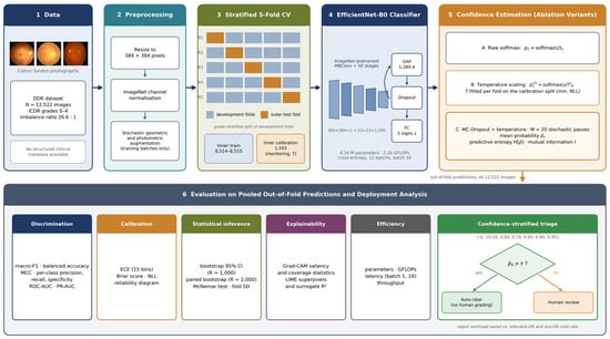
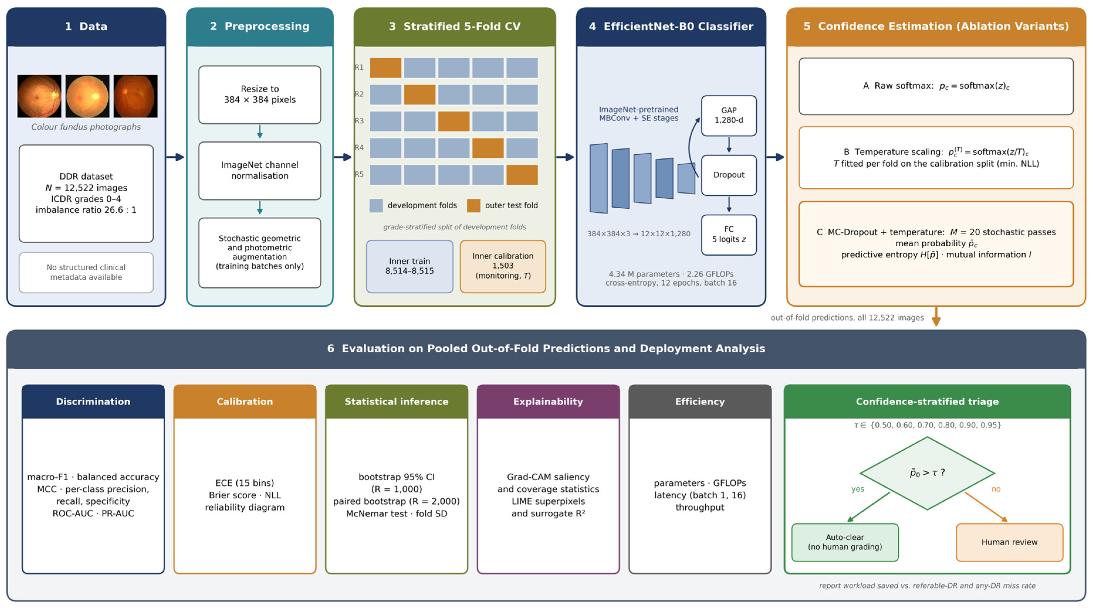
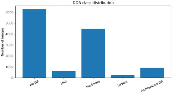
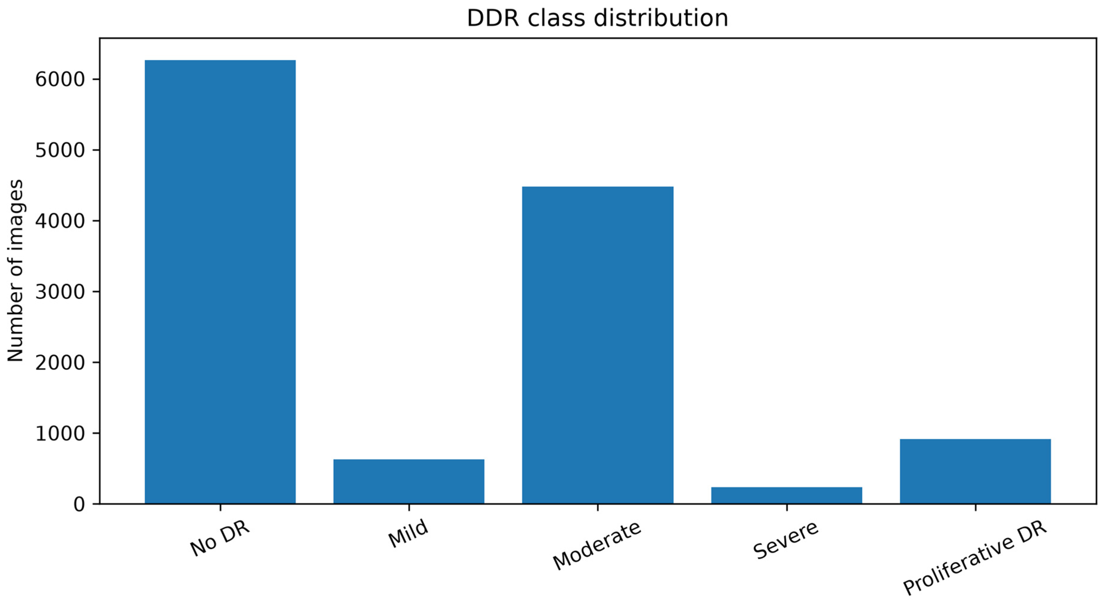
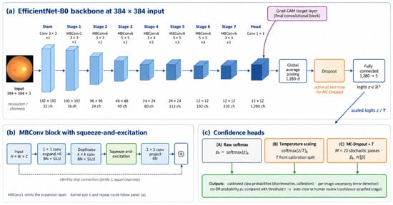
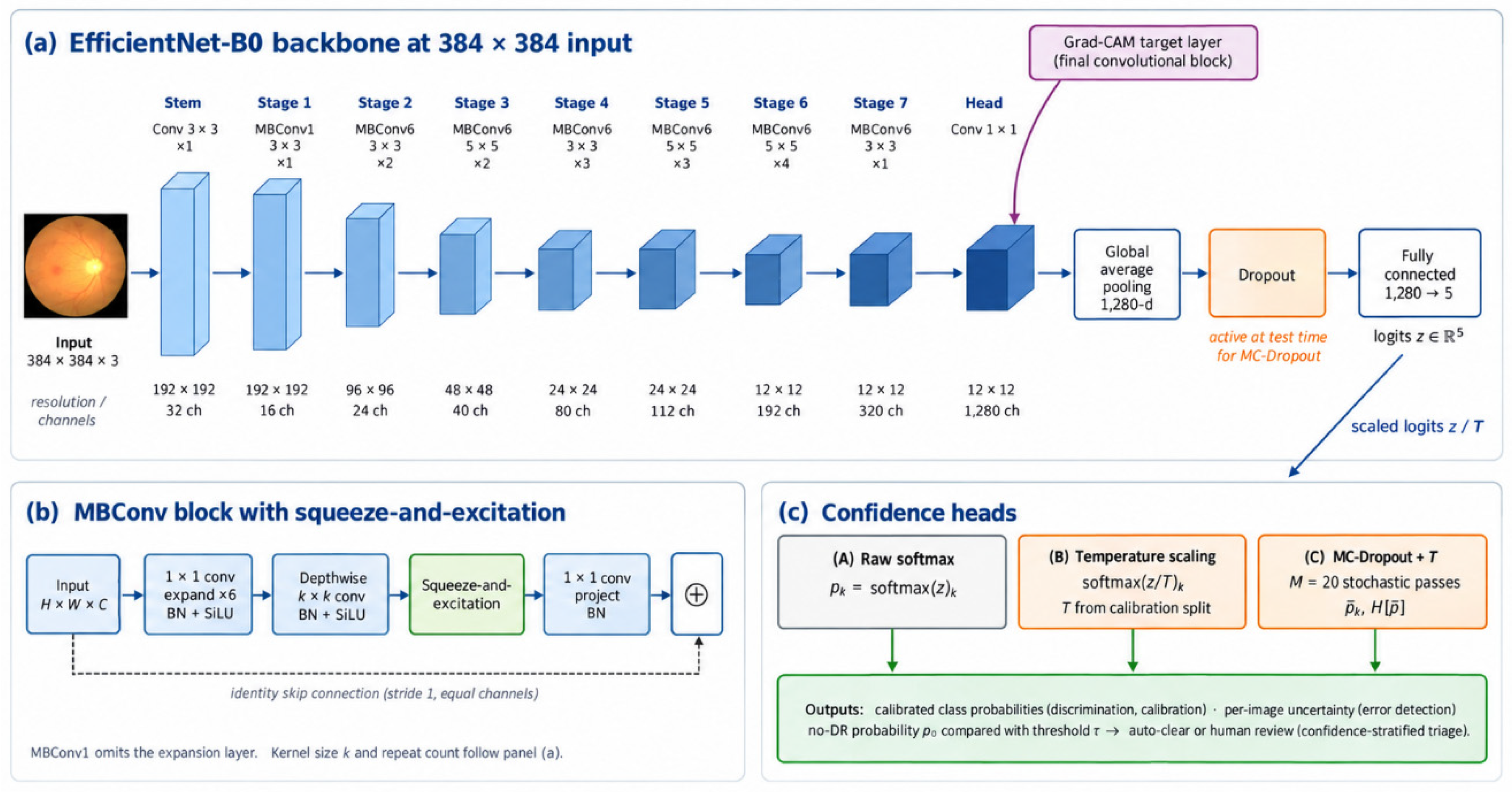
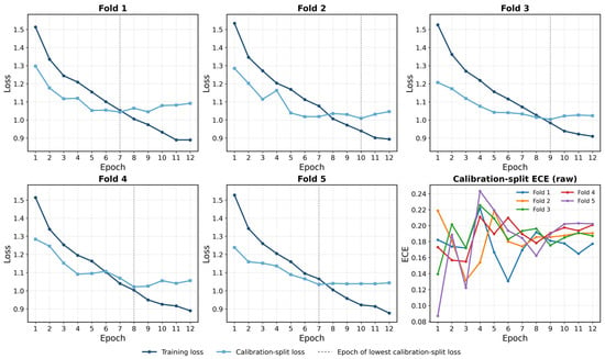
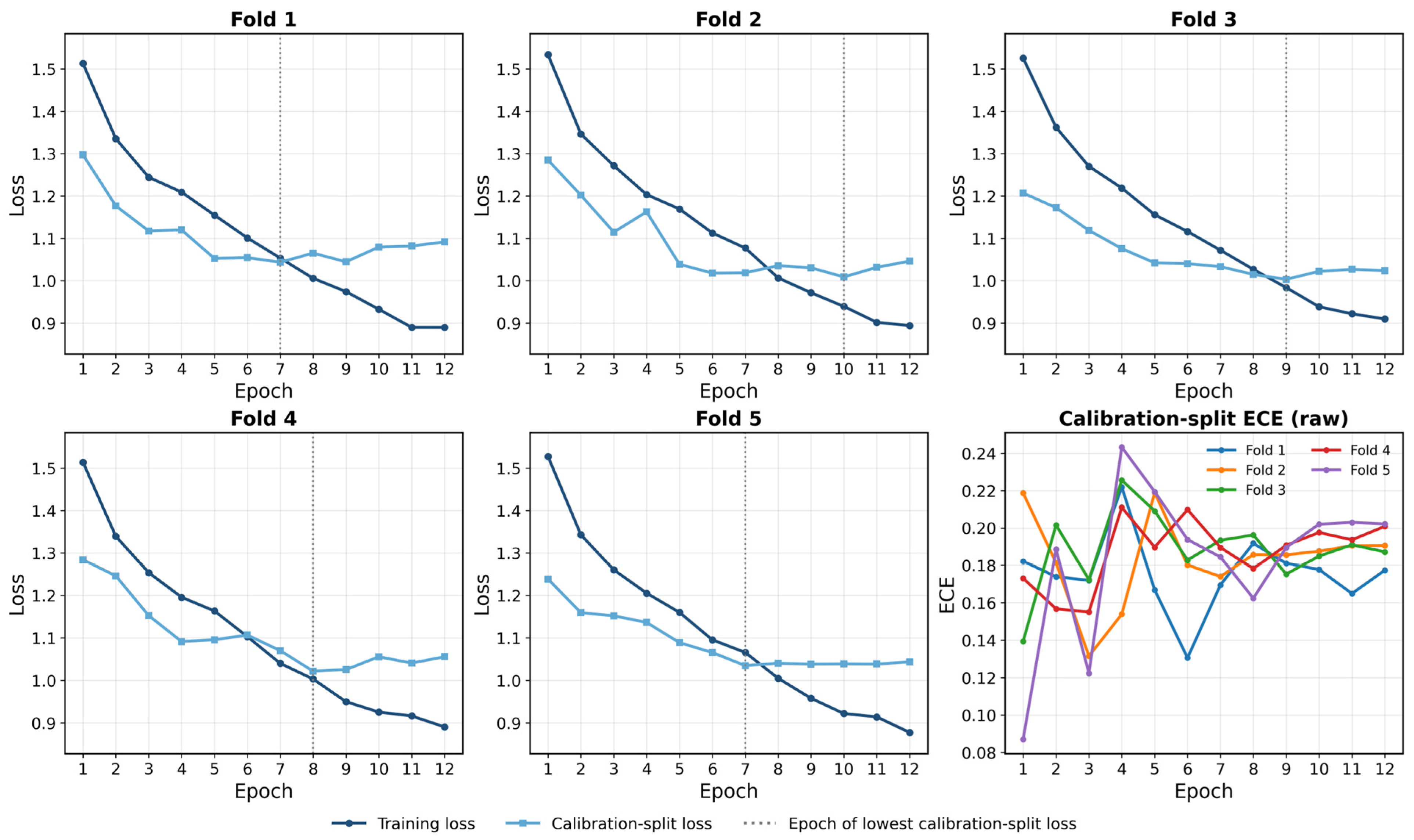
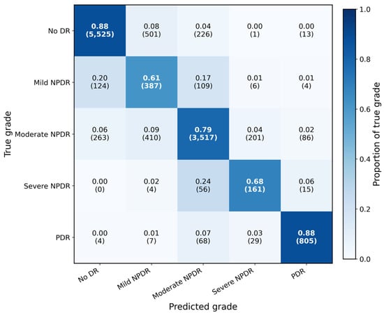
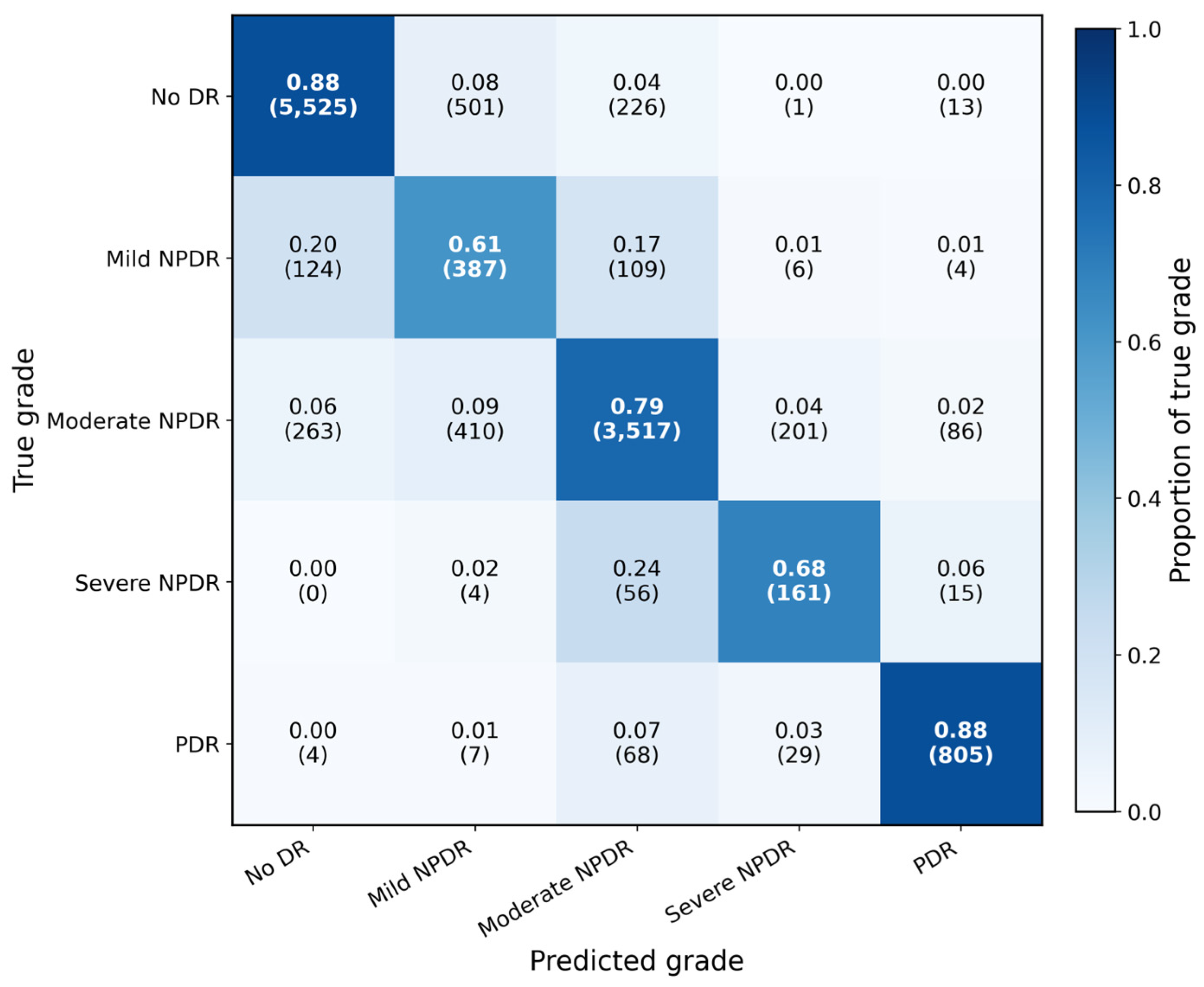
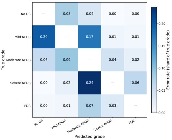
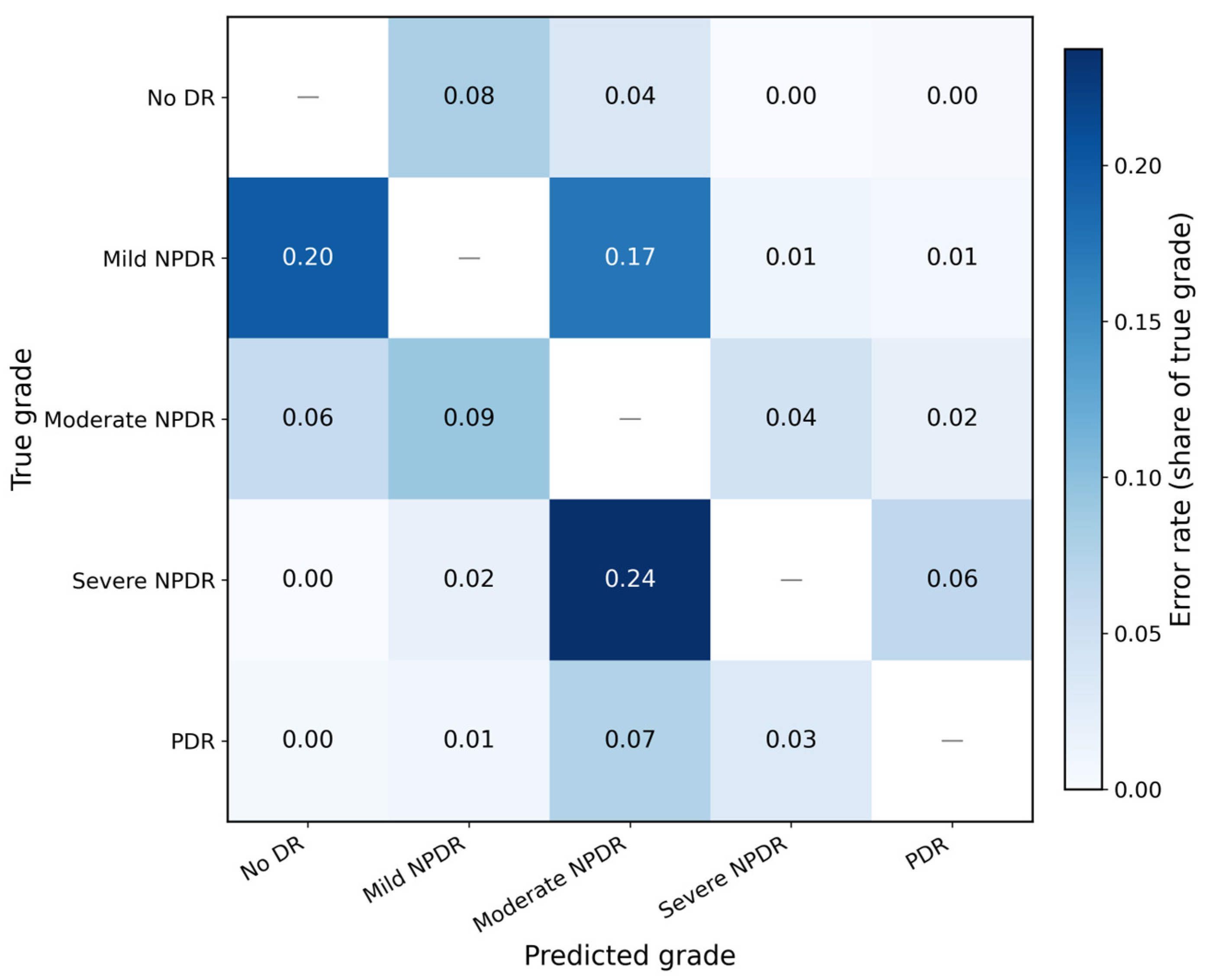
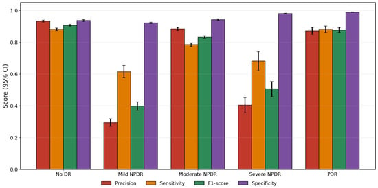
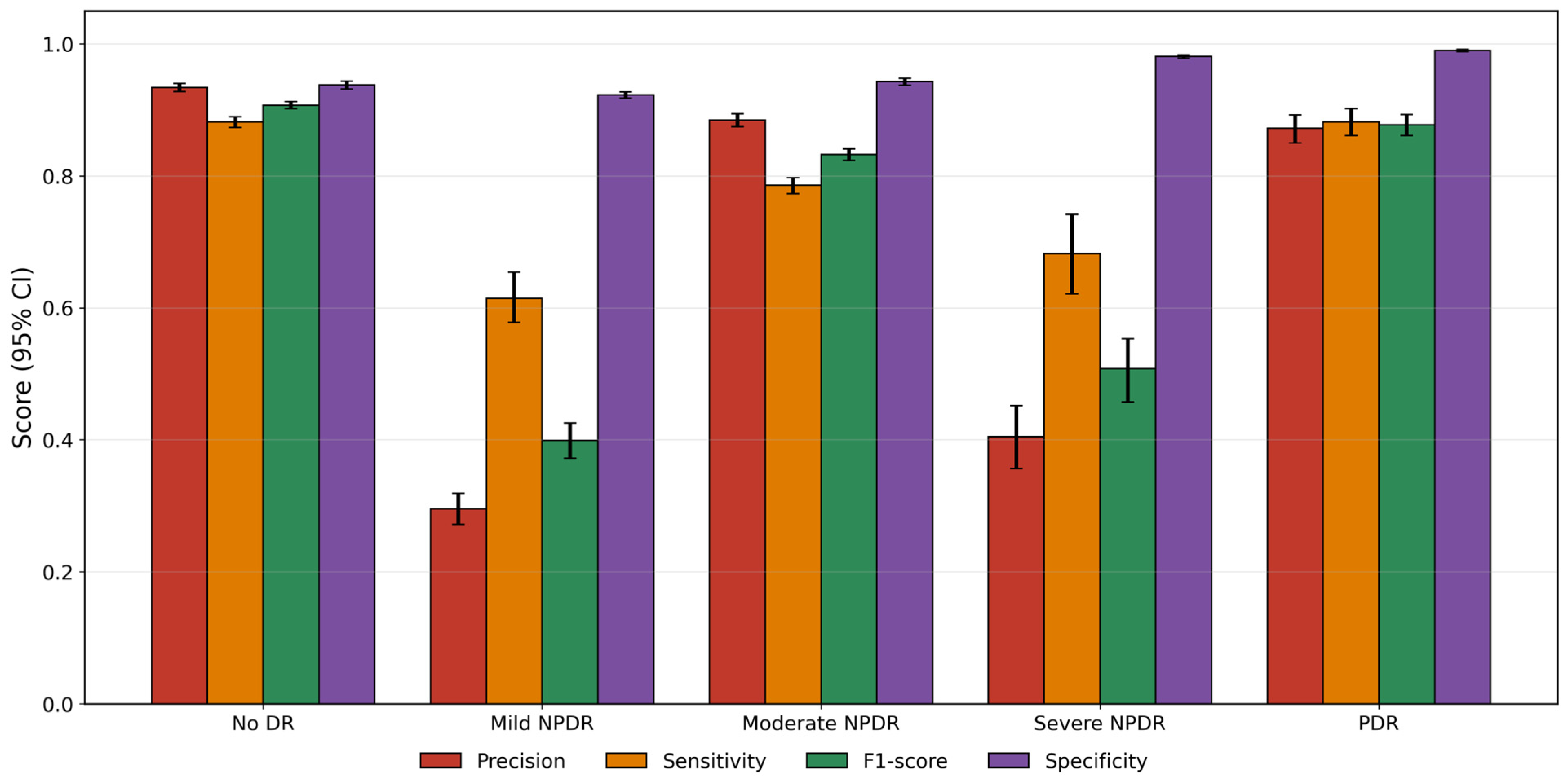
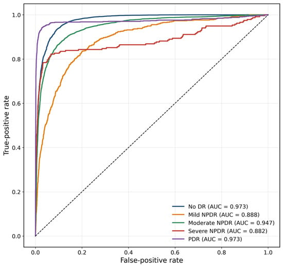
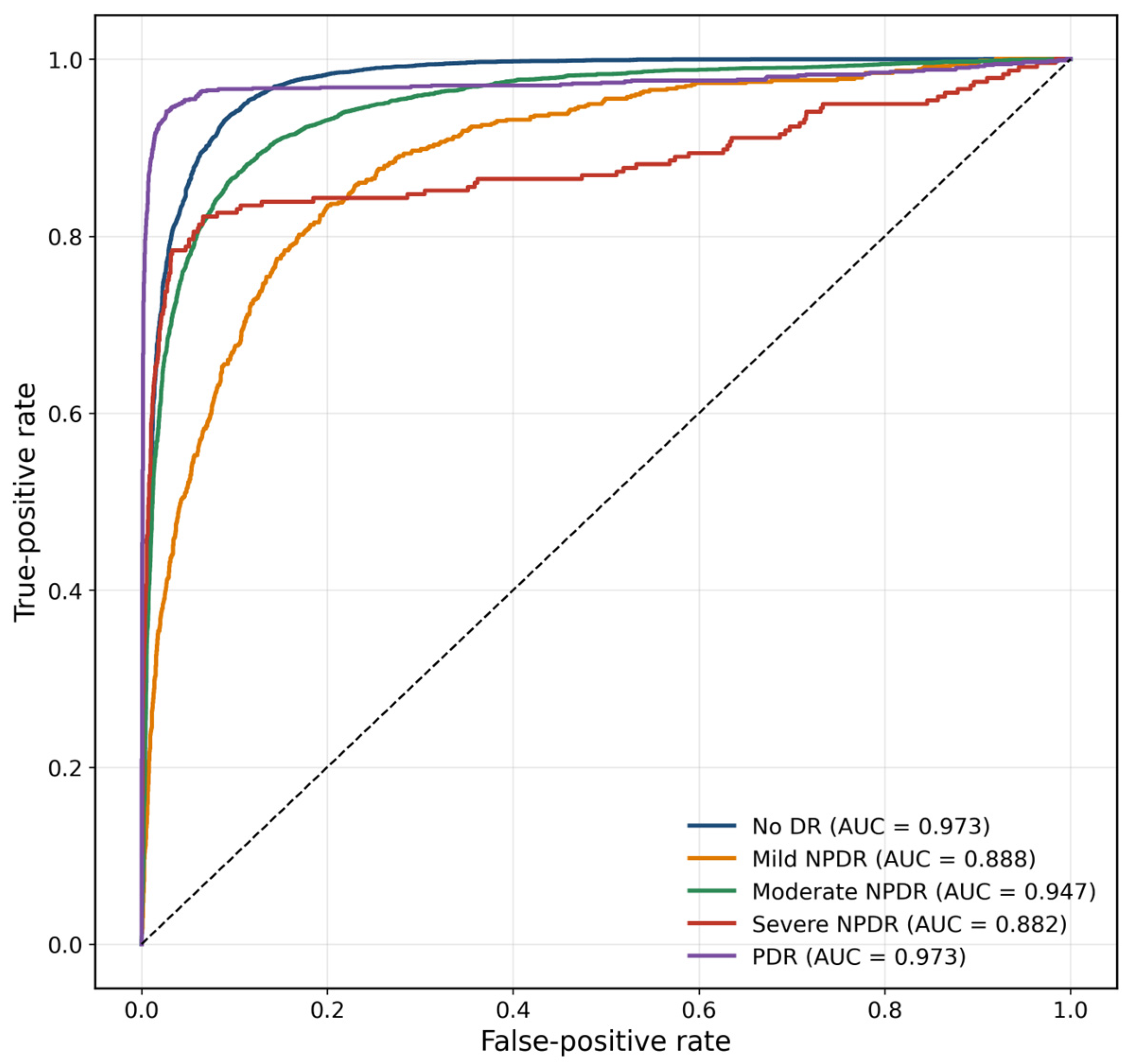
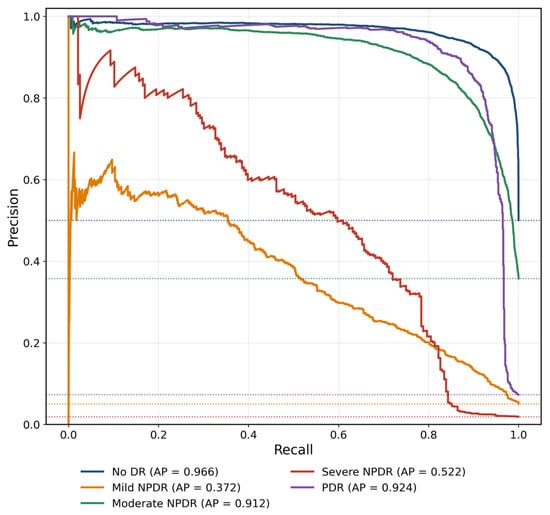
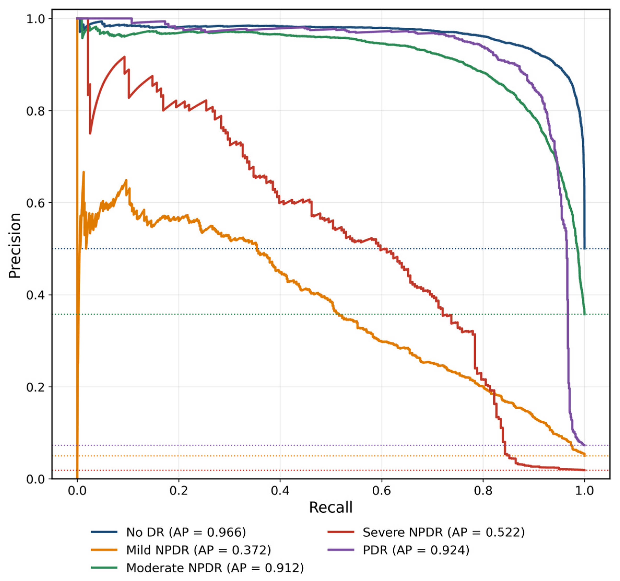
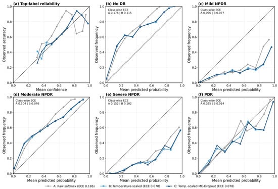
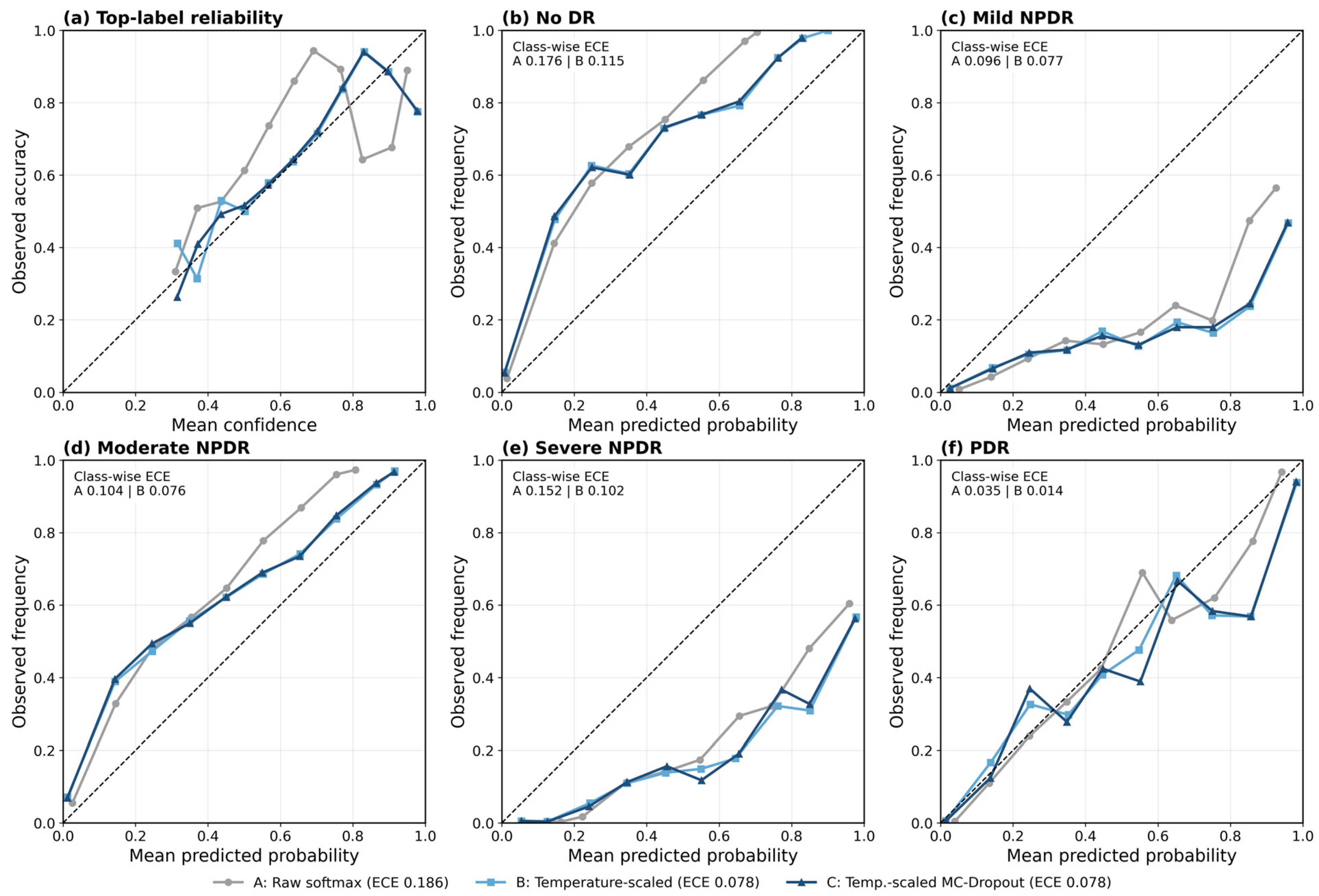
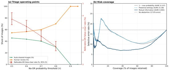
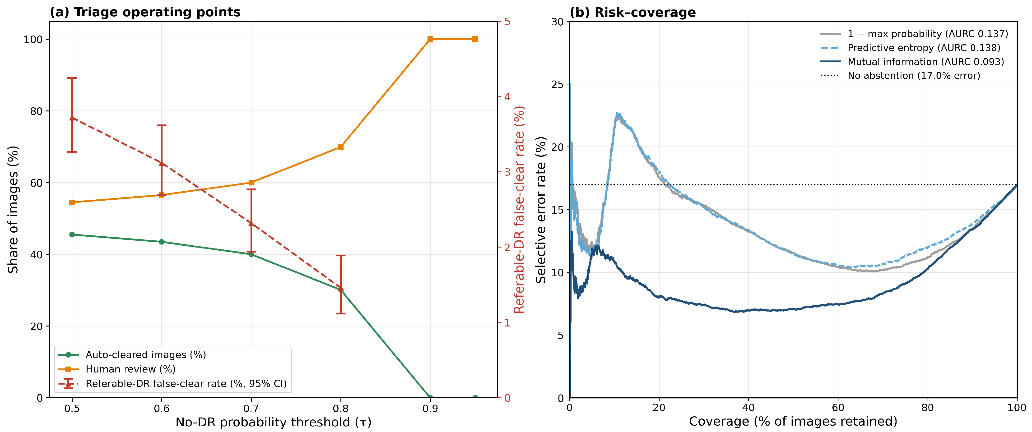
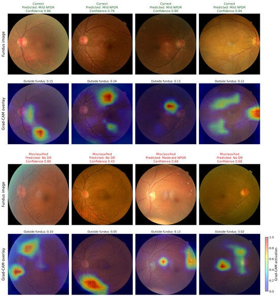
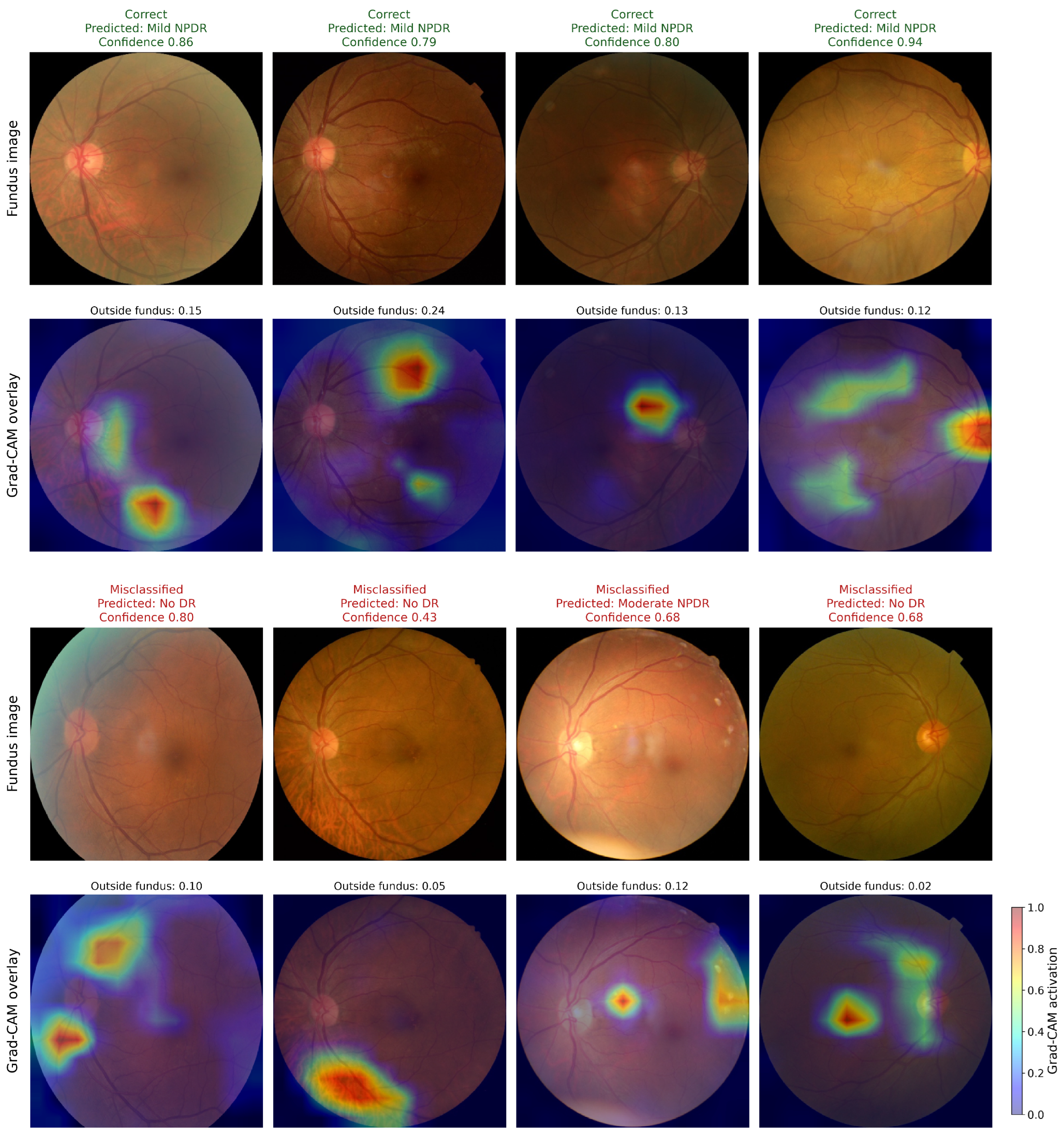
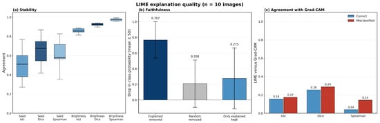
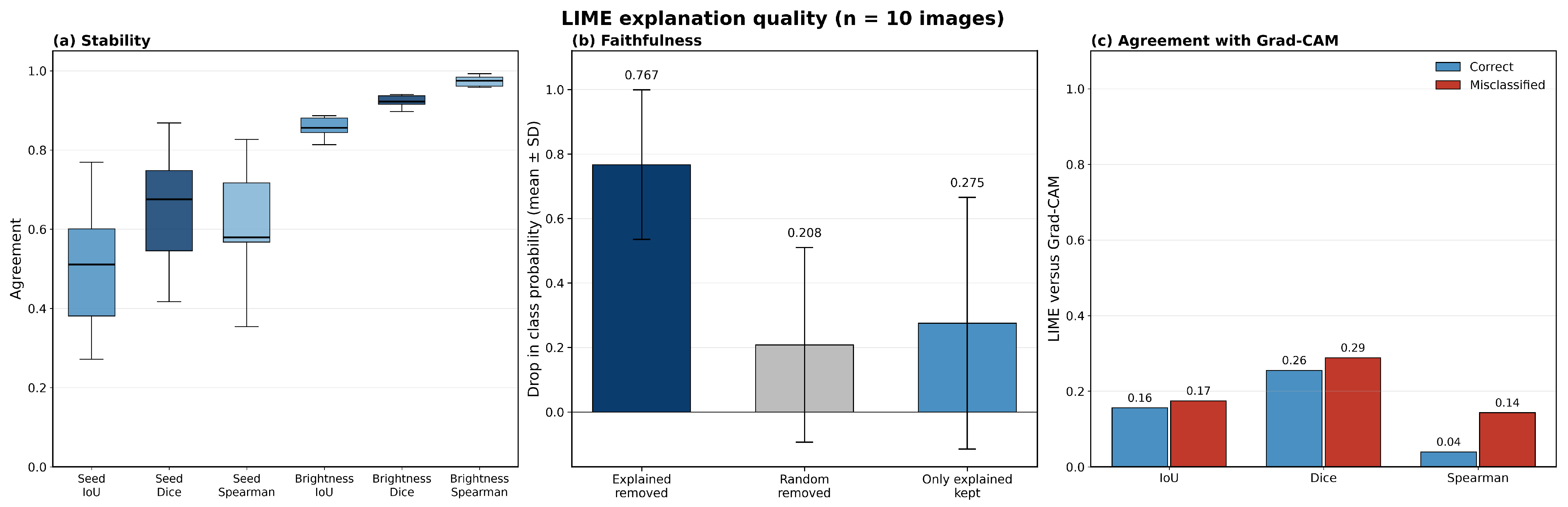
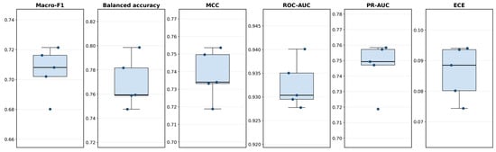
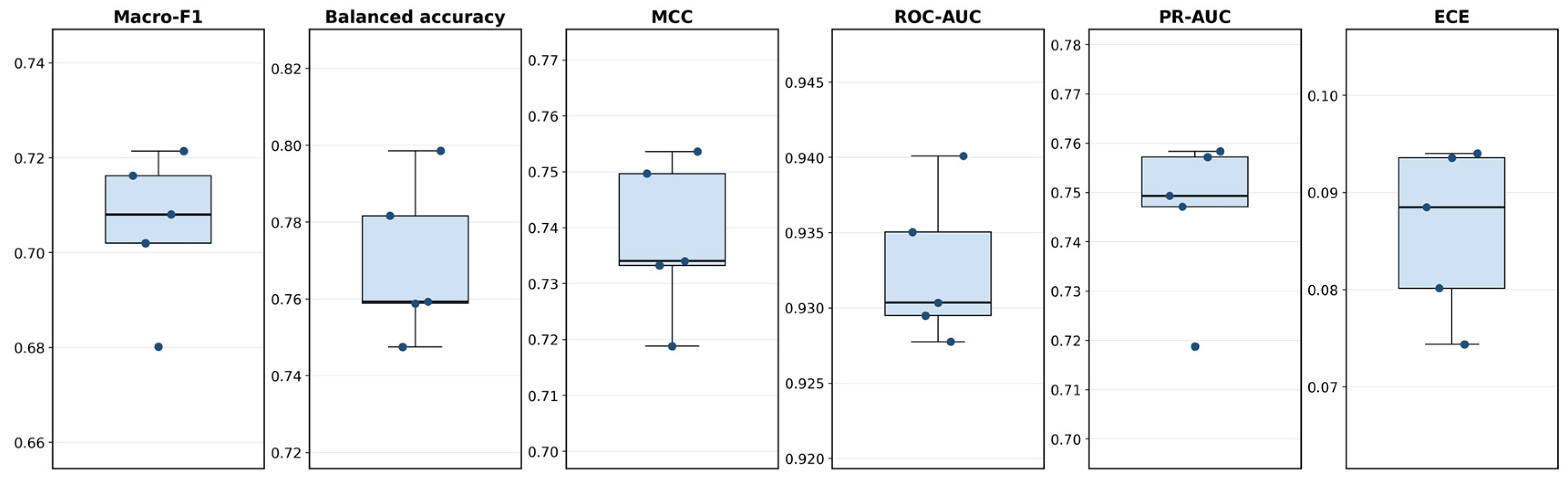
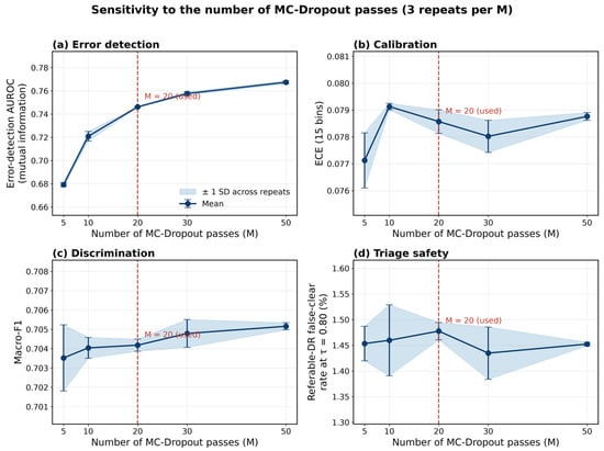
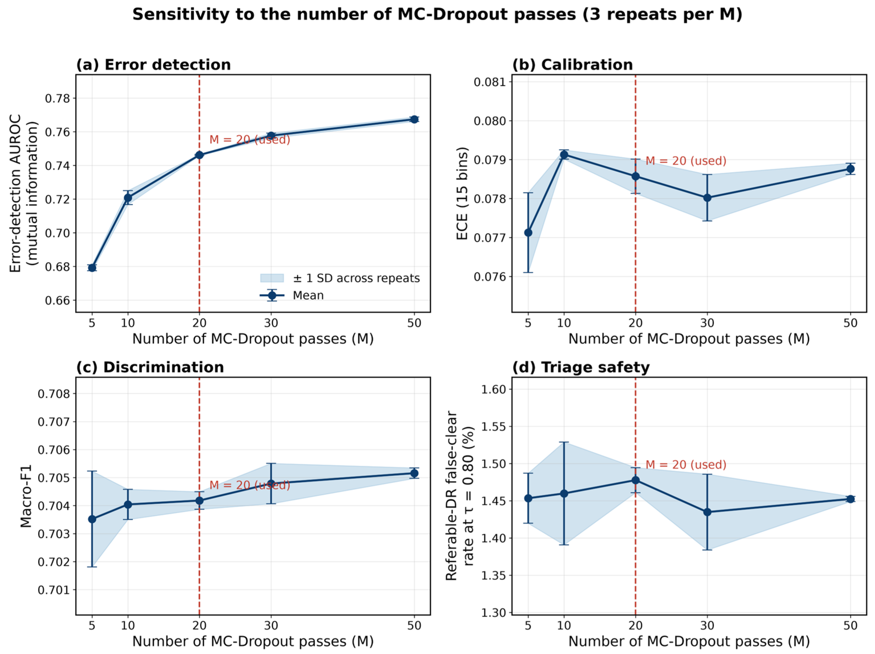
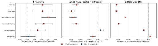
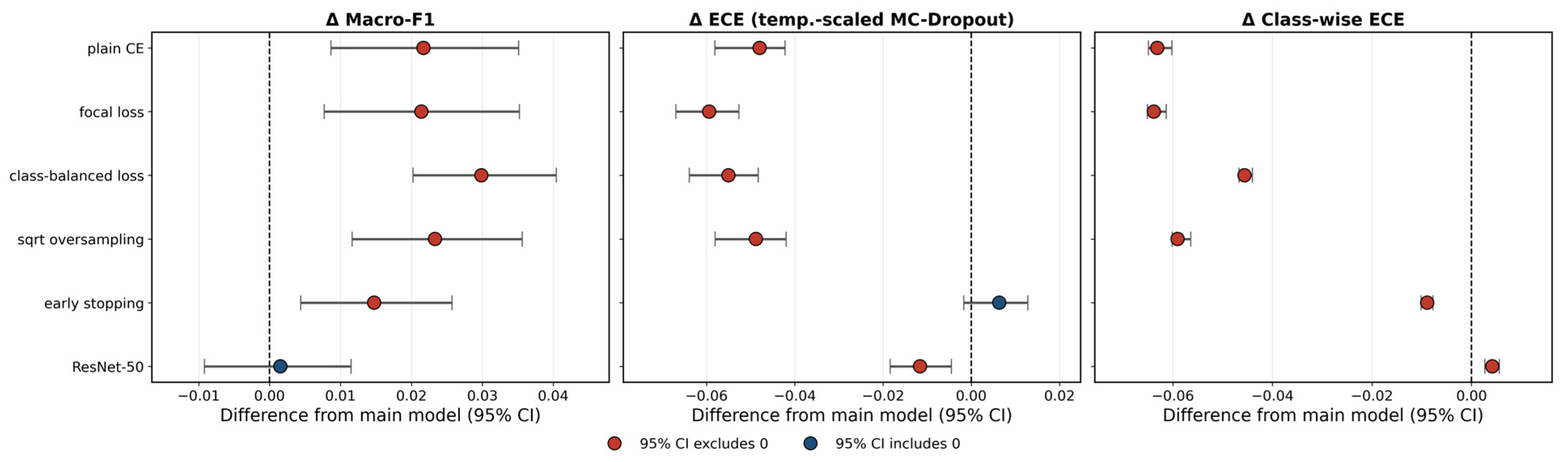

Disclaimer/Publisher’s Note: The statements, opinions and data contained in all publications are solely those of the individual author(s) and contributor(s) and not of MDPI and/or the editor(s). MDPI and/or the editor(s) disclaim responsibility for any injury to people or property resulting from any ideas, methods, instructions or products referred to in the content. |
© 2026 by the authors. Licensee MDPI, Basel, Switzerland. This article is an open access article distributed under the terms and conditions of the Creative Commons Attribution (CC BY) license.